Embed Size (px)
Citation preview

Trajectory Planners forCooperative Control of Two
Industrial Robots and Belt Drives
by
T.S.S. Jayawardene
M.Sc. in Operational Research, 2003
A dissertation submitted in partial fulfillment ofthe requirements for the Doctor of Philosophy
degree in Advanced Systems Control Engineering,Graduate School of Science and Engineering,
Saga University
March, 2005
Supervisor: Professor Masatoshi Nakamura
i
Abstract
This thesis focuses on trajectory planning strategies for high-speed, vibrationrestrained position control of belt drives and cooperative contour control of two robotsin view of increasing the speed of cooperative task. The proposed solutions have beendevised, implemented and verified for effective functionality. The trajectory planningin this context is carried out considering the relevant kinematic constraints met inactual practice; the maximum joint velocity constraints and the maximum joint accel-eration constraints. The proposed planners are based on the principles of kinematicsand the trajectory planning scenarios and, the issues are critically reviewed.
For belt driven machine, a fourth order kinematic model integrating belt reac-tion torque is systematically derived, and thereby explained the spiky phenomenonin velocity profile of motor position, when an acceleration change is experienced.Further, a feed forward dynamic compensator is proposed to restraint vibration andto improve dynamic characteristics of the belt drives. The proposed feed forwardcompensator is a combination of inverse dynamics of the system and a desirable dy-namic filter, which reforms the dynamic characteristics of the existing system. Theplanned trajectories at low speeds and high speeds are extensively tested for accurateperformance with an actual belt driven machine and the results are illustrated.
The proposed trajectory planners for two-robot cooperation are basically oftwo types. 1) Given objective cooperative trajectory exceeding the dynamic boundsof a single robot is decomposed into two concurrent complementary trajectories oftwo robots maneuvered simultaneously 2) For a specified objective locus, the min-imum time complementary trajectories for cooperation are planned. The objectivelocus used to exemplify the concept of trajectory planners in both cases is an S-shaped locus and realization of the trajectories are carried out under maximum jointacceleration constraints. In the former cooperative trajectory planner, a fair task dis-tribution is accomplished by minimizing the difference in maximum joint velocitiesof two robots. The complexities in planning trajectories are coped with a two-stagetrajectory-planning paradigm backed with a short-listing criterion. A fourth orderspline technique for position, minimizing the joint acceleration is also derived theo-retically. The latter, minimum time cooperative trajectory planner, is of bang-bangtype in acceleration profile and the fairness of each robot contribution is achievedthrough an additional contribution constraint for each robot to the cooperative task.The applicability of the trajectory-planning concept has been verified with coopera-tive trajectories having sharp corners.
Since the proposed trajectory planners concerned under the thesis work areoff-line and therefore they can be conveniently applied to existing servo systems irre-spective of the computational power of in-use controller. Neither, a dramatic changein the existing hardware setup nor a considerable reconfiguration of the system isdemanded in instrumentation point of view. This requirement of minimal changes inadaptation enhances the pragmatic significance of the proposed schemes.
ii

Approval
Graduate School of Science and EngineeringSaga University
1-Honjomachi, Saga 840-8502, Japan
CERTIFICATE OF APPROVAL
Ph.D. Dissertation
This is to certify that the Ph.D. Dissertation of
T.S.S. Jayawardene
B.Sc. Engineering in Electronics and Telecommunication Engineering, 1996M.Sc. in Operational Research, 2003
has been approved by the Examining Committeefor the dissertation requirement for the Doctor of Philosophydegree in Robotics and Systems Controlat the March, 2005 graduation.
Dissertation committee:Supervisor, Prof. Masatoshi NakamuraDept. of Advanced Systems Control Engineering
Member, Prof. Katsunori ShidaDept. of Advanced Systems Control Engineering
Member, Prof. Keigo WatanabeDept. of Advanced Systems Control Engineering
Member, Assoc. Prof. Satoru GotoDept. of Advanced Systems Control Engineering
iii

Copyright c©
Copyright c© March, 2005
by
T.S.S. JayawardeneAll Rights Reserved
iv

Dedication
To my loving, courageous mother, uncle, auntand
To all my loving teachers
v

Acknowledgements
First and foremost, the author expresses his heartfelt gratitude to his supervisoras well as academic advisor, Professor Masatoshi Nakamura for valuable guidance, hissuggestions and encouragement. It has been so indispensable throughout the recentthree years of his academic and research carrier in Saga University, Japan. ProfessorMasatoshi Nakamura has been more than an academic supervisor. He showed a welldisciplined thinking pattern which conditioned his students in such a way they begood people in the society. It is both a privilege and a pleasure to be his student.The author owes a debt of gratitude to Associate Professor Satoru Goto for kindassistance, his guidance and support given while being one of his supervisors.
The author would be very grateful to the members of the dissertation commit-tee, Professor Katsumori Shida, Professor Keigo Watanabe, and Associate ProfessorSatoru Goto for wading through numerous drafts of this document. Their insightcontributed through comments and suggestions has been very helpful.
The author extends sincere gratitude to his scholarship donor, Science and Tech-nology personnel development project of The Government of Sri Lankan on ADBloan. The author would like to thank Saga University for the financial support giventhrough research/teaching assistanceship and for providing an invigorating environ-ment to explore new ideas. The author expresses his great gratitude to Dr. Indral-ingm, the former head of the Department of Mathematics, University of Moratuwaand to Dr. Chandana Perera, a senior lecturer in the Department of Managementof Technology, University of Moratuwa for being the supervisors to M.Sc. in Opera-tional Research. Their guidance, support and encouragement in the master’s studiesimmensely help to make the headway towards the doctoral studies. The colleaguestaff members of the university of Moratuwa, especially Dr. Nirmali de Silva and Mr.N.L. Wanigatunga (the former and the current head of the Department of Textilesand clothing Technology, University of Moratuwa) are also reminded with a greatgratitude and a grateful feeling as they basically facilitated the logistics of the higherstudy opportunity in Saga University.
The author expresses his gratitude to Professor Nobuhiro Kyura, Department ofElectrical Engineering, Kinki University (in Kyushu), for his constructive commentsand inspiring ideas. A special thank conveys to Dr. N. Egashira, Kurume Institute ofTechnology and Professor S. Nishida, Fukuoka Institute of Technology for the valu-able comments and remarks made in research discussions.
The author has had great discussions with Rohan Munasinghe, Koliya Pulas-inghe, Sisil Kumarawadu, Lanka Udawatta, Chandimal Sanjeeva, Liu Peng, DaisukeKushida and Tao Zang. These discussions have had profound impact on the ideasof this thesis. Duminda Nishantha helped the author to tackle few tough spots ofcoding through imparting modern programming techniques and coding paradigms.
The author is greatly indebted to Ms. Masuda Chizuko, who taught Japanese
vi

vii
language and thereby paved the way to accustom to Japanese society. She deservesthe warmest gratitude for the persistent support and kind assistance provided to rec-ognize the cultural norms, which are essential to lead a comfortable and enjoyable lifein Japan. She supported the author in all exigency needs and became “a mother inJapan” to the author. Youth Federation for World Peace (YFWP) and Saga Prefec-ture International Relationship Association (SPIRA) must be thanked for organizinginternational sports events, in which the author participates and makes his life en-joyed with extra curricular activities. The author shows his gratefulness to SPIRAfor their kind assistance and cooperation received. And of course, the author doesnot forget to remember his mother, uncle, aunt and sisters who have all stood stillwith him through the best of times and the worst of times. Their unconditional loveand support have helped me to get through some very difficult times. So the authordoes his best to give them a reason to be proud of.
The author extends his sincere thanks to Lecturer Dr. T. Sugi, Mr. K. Naga-fuchi, Technician, Ms. M. Egashira and M. Iwanaga, Secretaries of the AdvancedSystems Control Engineering Laboratory, for the generosity and assistance giventhroughout his stay in Japan. Author also extends his heartfelt gratitude to hiscolleagues of the Advanced Systems Control Engineering Laboratory, Saga Univer-sity for their great company and indispensable assistance, which helped him to adoptJapanese society and culture. He remembers all his Japanese and Sri Lankan friendswith a lovely and grateful feeling.

Contents
Page
Title . . . . . . . . . . . . . . . . . . . . . . . . . . . . . . . . . . . . . . . iAbstract . . . . . . . . . . . . . . . . . . . . . . . . . . . . . . . . . . . . . iiApproval . . . . . . . . . . . . . . . . . . . . . . . . . . . . . . . . . . . . . iiiDedication . . . . . . . . . . . . . . . . . . . . . . . . . . . . . . . . . . . . vAcknowledgements . . . . . . . . . . . . . . . . . . . . . . . . . . . . . . . viiList of Figures . . . . . . . . . . . . . . . . . . . . . . . . . . . . . . . . . . xiList of Tables . . . . . . . . . . . . . . . . . . . . . . . . . . . . . . . . . . xiii
Chapter
1 Introduction 11.1 Background . . . . . . . . . . . . . . . . . . . . . . . . . . . . . . . . . . 1
1.1.1 Brief history and robot definition . . . . . . . . . . . . . . . . . 11.1.2 Constructional details and robot classifications . . . . . . . . . . 11.1.3 Industrial Applications of Robots . . . . . . . . . . . . . . . . . 31.1.4 Introduction to trajectory planning . . . . . . . . . . . . . . . . 51.1.5 Overview of trajectory planning algorithms and characteristics . 7
1.2 Literature Review . . . . . . . . . . . . . . . . . . . . . . . . . . . . . . 81.2.1 Belt drives . . . . . . . . . . . . . . . . . . . . . . . . . . . . . . 81.2.2 Trajectory planning strategies and cooperative planning . . . . 9
1.3 Motivation . . . . . . . . . . . . . . . . . . . . . . . . . . . . . . . . . . 111.3.1 Belt driven machine . . . . . . . . . . . . . . . . . . . . . . . . . 111.3.2 Cooperative control . . . . . . . . . . . . . . . . . . . . . . . . . 11
1.4 Contributions of the Thesis . . . . . . . . . . . . . . . . . . . . . . . . . 121.4.1 Belt driven systems . . . . . . . . . . . . . . . . . . . . . . . . . 121.4.2 Cooperative trajectory planners . . . . . . . . . . . . . . . . . . 121.4.3 Scope of application . . . . . . . . . . . . . . . . . . . . . . . . . 13
1.5 A Preview: Outline of the Thesis . . . . . . . . . . . . . . . . . . . . . . 13
2 Belt Driven Machine 152.1 Preliminaries . . . . . . . . . . . . . . . . . . . . . . . . . . . . . . . . . 15
2.1.1 Characteristics of belt drives . . . . . . . . . . . . . . . . . . . . 152.1.2 Experimental setup and schematics of belt driven machine . . . 15
2.2 Problem Statement and Planning Algorithm . . . . . . . . . . . . . . . 162.2.1 Problem statement . . . . . . . . . . . . . . . . . . . . . . . . . 162.2.2 Trajectory planning algorithm and overview of compensation . . 17
2.3 Spiky Phenomenon in Velocity Profile of Belt Drives . . . . . . . . . . . 182.4 Proposed Model and Solution Strategy for Belt Driven Machine . . . . . 19
2.4.1 Rationale . . . . . . . . . . . . . . . . . . . . . . . . . . . . . . . 192.4.2 Model construction . . . . . . . . . . . . . . . . . . . . . . . . . 202.4.3 Modified taught data technique . . . . . . . . . . . . . . . . . . 222.4.4 Design of Feed Forward Compensator . . . . . . . . . . . . . . . 232.4.5 Analytical solutions . . . . . . . . . . . . . . . . . . . . . . . . . 24
2.5 Performance and Evaluation . . . . . . . . . . . . . . . . . . . . . . . . 262.6 Concluding Remarks . . . . . . . . . . . . . . . . . . . . . . . . . . . . . 27
viii

Contents ix
3 Dual Arm Trajectory Planning for a Specified Cooperative Trajectory 303.1 Cooperative Control . . . . . . . . . . . . . . . . . . . . . . . . . . . . . 30
3.1.1 Definition and categorization of cooperative control . . . . . . . 303.1.2 Cooperative control research directions . . . . . . . . . . . . . . 313.1.3 Concept of cooperative control . . . . . . . . . . . . . . . . . . . 32
3.2 Preliminaries . . . . . . . . . . . . . . . . . . . . . . . . . . . . . . . . . 333.2.1 System overview . . . . . . . . . . . . . . . . . . . . . . . . . . . 333.2.2 Coordinate transformation . . . . . . . . . . . . . . . . . . . . . 333.2.3 Significance of piecewise linear off-line trajectory planning . . . . 34
3.3 Problem Statement . . . . . . . . . . . . . . . . . . . . . . . . . . . . . 353.4 Two Stage Trajectory-Planning Paradigm . . . . . . . . . . . . . . . . . 36
3.4.1 Rationale . . . . . . . . . . . . . . . . . . . . . . . . . . . . . . . 363.4.2 Realization of cooperative control . . . . . . . . . . . . . . . . . 373.4.3 Trajectory generation criterion . . . . . . . . . . . . . . . . . . . 383.4.4 Segment Level Trajectory Planning . . . . . . . . . . . . . . . . 403.4.5 Short listing criterion . . . . . . . . . . . . . . . . . . . . . . . . 413.4.6 Coarse to fine trajectory planning refinement . . . . . . . . . . . 423.4.7 Optimal interpolation scheme . . . . . . . . . . . . . . . . . . . 42
3.5 RT-Linux for Real Time Operation . . . . . . . . . . . . . . . . . . . . . 443.6 Performance and Evaluation . . . . . . . . . . . . . . . . . . . . . . . . 453.7 Concluding Remarks . . . . . . . . . . . . . . . . . . . . . . . . . . . . . 46
4 Minimum Time Cooperative Control of Two Robots 554.1 Preliminaries . . . . . . . . . . . . . . . . . . . . . . . . . . . . . . . . . 55
4.1.1 Prelude to minimum time cooperative control . . . . . . . . . . 554.1.2 Cartesian robot configuration . . . . . . . . . . . . . . . . . . . 554.1.3 Parameterization of objective locus . . . . . . . . . . . . . . . . 574.1.4 Physical coordinate to cooperative coordinate mapping . . . . . 57
4.2 Generic Form Problem Statement . . . . . . . . . . . . . . . . . . . . . 584.3 Time Optimal Cooperative Trajectory Generation . . . . . . . . . . . . 59
4.3.1 Design issues of minimum time cooperative control algorithm . . 594.3.2 Proposed trajectory planning algorithm . . . . . . . . . . . . . . 60
4.4 Theoretical Aspects of the Proposed Algorithm . . . . . . . . . . . . . . 624.4.1 Philosophical notions . . . . . . . . . . . . . . . . . . . . . . . . 624.4.2 No solution condition . . . . . . . . . . . . . . . . . . . . . . . . 654.4.3 Progressive mode and advancing through fold back mode . . . . 66
4.5 Appraisal of Planned Cooperative Trajectory . . . . . . . . . . . . . . . 674.6 Concluding Remarks . . . . . . . . . . . . . . . . . . . . . . . . . . . . . 68
5 Conclusions and Recommendations 745.1 Conclusions . . . . . . . . . . . . . . . . . . . . . . . . . . . . . . . . . . 745.2 Significant Remarks . . . . . . . . . . . . . . . . . . . . . . . . . . . . . 755.3 Recommendations for Further Developments . . . . . . . . . . . . . . . 76
5.3.1 Belt driven machine . . . . . . . . . . . . . . . . . . . . . . . . . 775.3.2 Cooperative trajectory planner for a given objective trajectory . 785.3.3 Minimum time cooperative trajectory planner of two Cartesian
robots under given objective locus . . . . . . . . . . . . . . 79
Appendices 80
A Coordinate Systems and Transformations 80A.1 Coordinate Systems for Spatial Description . . . . . . . . . . . . . . . . 80A.2 Mathematical Representation and Operations . . . . . . . . . . . . . . . 80

x Contents
B Space Transformation 82B.1 Forward Kinematics and Inverse Kinematics . . . . . . . . . . . . . . . . 82
C An Overview of Robot Manipulator System 84C.1 Schematic Representation of Robot System . . . . . . . . . . . . . . . . 84C.2 Specifications of a Typical Industrial Robot . . . . . . . . . . . . . . . . 84C.3 Coding Architecture of a Revolute Joint . . . . . . . . . . . . . . . . . . 85
D Famous Kinematic Models of Robot Systems 87D.1 First Order Kinematic Model . . . . . . . . . . . . . . . . . . . . . . . . 87D.2 Second Order Kinematic Model . . . . . . . . . . . . . . . . . . . . . . . 88D.3 Fourth Order Kinematic Model . . . . . . . . . . . . . . . . . . . . . . . 88
E Generation of Minimum Time Trajectory for a Single Robot 90
F Glossary of Terms 92
Publications 97
References 98

List of Figures
Figure Page
1.1 Anatomical Categorization of Robots . . . . . . . . . . . . . . . . . . . . . 21.2 Few Industrial Applications of Robots . . . . . . . . . . . . . . . . . . . . 41.3 Three Layer Hierarchical Model of Trajectory Planning and Controlling . . 72.1 Experimental Setup of Belt Driven Machine . . . . . . . . . . . . . . . . . 152.2 Schematic Diagram of Belt driven Machine . . . . . . . . . . . . . . . . . . 162.3 Objective Velocity Profile for Belt Driven Machine Control . . . . . . . . . 172.4 Trajectory Generation Criterion for Trapezoidal Velocity Profile . . . . . . 182.5 Spiky Phenomenon in Velocity Profile of Belt Driven Machine . . . . . . . 192.6 Flexible Structure of Belt Drive . . . . . . . . . . . . . . . . . . . . . . . . 212.7 Fourth Order Model of Belt Driven Machine . . . . . . . . . . . . . . . . . 222.8 Concept of Modified Taught Data Technique . . . . . . . . . . . . . . . . . 232.9 Dynamic Compensator for Data Modification . . . . . . . . . . . . . . . . 23
2.10 Simulation and Experiment Results of Belt Driven Machine . . . . . . . . 262.11 Comparison of Load Position Error . . . . . . . . . . . . . . . . . . . . . . 272.12 Simulation Results of Load Tracking . . . . . . . . . . . . . . . . . . . . . 282.13 Multi-axis Belt Driven Manipulator . . . . . . . . . . . . . . . . . . . . . . 293.1 Concept of Cooperative Control . . . . . . . . . . . . . . . . . . . . . . . . 323.2 Experiment Setup Illustrating Two-Robot Manipulator Configuration . . . 333.3 Realization of Cooperative Control . . . . . . . . . . . . . . . . . . . . . . 373.4 State Tree of Global Solution Space . . . . . . . . . . . . . . . . . . . . . . 383.5 Entire Trajectory Generation Algorithm . . . . . . . . . . . . . . . . . . . 493.6 Algorithm for the Generation of Feasible Solution . . . . . . . . . . . . . . 503.7 Fine Details of Joint Velocity Curves: Inter-Intra Segments . . . . . . . . . 503.8 Detailed Architecture of RT-Linux Kernel . . . . . . . . . . . . . . . . . . 513.9 Coarse Level Input Trajectory Prior to Interpolation . . . . . . . . . . . . 51
3.10 Fine Level Input Trajectory after Interpolation . . . . . . . . . . . . . . . 523.11 Experiment Results of Two Robot Trajectories . . . . . . . . . . . . . . . . 523.12 Simulation Results with Two Robot Output Trajectories . . . . . . . . . . 533.13 Objective and Cooperative Trajectories of Simulation and Experiment . . . 533.14 Experimental Results of Minimum Time Mono Robot Trajectory Generated
under Acceleration Constraint . . . . . . . . . . . . . . . . . . . . . . 543.15 Comparison of Simulation Error in Workspace . . . . . . . . . . . . . . . . 544.1 Definition of Physical Coordinate Systems . . . . . . . . . . . . . . . . . . 554.2 Definition of Cooperative Coordinate Systems and Parameterization of Locus 564.3 Timely Notation of Position Velocity and Acceleration . . . . . . . . . . . 564.4 Generic Form Objective Cooperative Locus . . . . . . . . . . . . . . . . . . 584.5 Entire Cooperative Trajectory Generation Criterion . . . . . . . . . . . . . 634.6 Algorithm for Calculation of Optimum Parameter Increment . . . . . . . . 644.7 Minimum Time Input Cooperative Trajectory of Two Cartesian Robots for
S-Shaped Locus . . . . . . . . . . . . . . . . . . . . . . . . . . . . . . 704.8 Minimum Time Input Joint Space Trajectory of Two Cartesian Robot for
V-Shaped Locus . . . . . . . . . . . . . . . . . . . . . . . . . . . . . . 704.9 Minimum Time Input Trajectory of Single Cartesian Robot for S-Shaped
Locus . . . . . . . . . . . . . . . . . . . . . . . . . . . . . . . . . . . 71
xi

xii List of Figures
4.10 Minimum Time Input Trajectory of Single Cartesian Robot for V-ShapedLocus . . . . . . . . . . . . . . . . . . . . . . . . . . . . . . . . . . . 71
4.11 Cumulative Contribution of Robot A in Cooperative Control of Two Carte-sian Robots for S-Shaped Locus . . . . . . . . . . . . . . . . . . . . . 72
4.12 Tangential Cooperative Velocity Profile for S-Shaped Locus . . . . . . . . . 724.13 Tangential and Cooperative Velocity Profiles for V-Shaped Locus . . . . . 734.14 V-Shaped Locus in Work Space . . . . . . . . . . . . . . . . . . . . . . . . 73A.1 Translation and Rotation of Coordinate Systems . . . . . . . . . . . . . . . 81B.1 Diagrammatic Representation of Robot’s Link Structure . . . . . . . . . . 83C.1 Schematics of a Typical Robot Manipulator System . . . . . . . . . . . . 84C.2 Coding Architecture of a Single Decoupled Servo Joint . . . . . . . . . . . 85D.1 First Order Representation of Mechatronic Servo System . . . . . . . . . . 87D.2 Second Order Representation of Mechatronic Servo System . . . . . . . . . 88D.3 Fourth Order Representation of Mechatronic Servo System . . . . . . . . . 89

List of Tables
Table Page
2.1 Parameter Values of Belt Driven Machine . . . . . . . . . . . . . . . . . . 263.1 Parameter Values of Cooperative Control of Two Articulated Robots . . . 463.2 Comparison of Results in Terms of Accuracy and Task Completion Time . 474.1 Path and Cooperative Trajectory Specification for S-Shaped Locus . . . . 674.2 Path and Cooperative Trajectory Specification for V-Shaped Locus . . . . 674.3 Comparison of Two Robot Cooperative Trajectory with Single Robot Tra-
jectory in Task Completion Time for Both Loci . . . . . . . . . . . . 68C.1 Control System Parameters . . . . . . . . . . . . . . . . . . . . . . . . . . 85
xiii

Chapter 1
Introduction
1.1 Background
1.1.1 Brief history and robot definition
History of modern industrial robot runs to early 1940s to the invention of “MachinaSpeculatrix” by Grey Walter and “Beast” by Johns Hopkins. The first robot companycalled Universal Automation, later shortened to unimation was established by Engle-berger, who was later called the father of robotics [1]. George Devol, who workedwith Engleberger, designed the first programmable robot called “unimates” in 1954and held the patent for the first industrial robot [2]. First ever computer controlledrobot was developed by Ernst at MIT in 1961 [3]. Concurrent dramatic developmentin robotics hardware and theoretical innovations makes robotics into a concrete disci-pline by itself. In 1980s robot industry entered a phase of rapid growth, when manyinstitutions introduced programs and courses in robotics.
The word “robot” came from the Czech word “robota” meaning forced labour,and Karel Capec coined it in 1923. There are many definitions suggested for industrialrobots and all of them encompass the notion of mobility, programmability and theuse of sensory feedback in determining subsequent behavior, though the word mayconjure up many levels of sophistications. For the sake of completeness, few populardefinitions are stated below.
An automatic device that performs functions normally ascribed to humans ormachine in the form of a human-Webster Dictionary [4].
A programmable multifunctional manipulator designed to move materials, parts,tools or specialized devices through various programmed motions for the performanceof a variety of tasks-Robot Institute of America [5].
1.1.2 Constructional details and robot classifications
Interconnection of links by different kinds of joints constitutes the mechanical struc-ture of the robot and it is an open kinematic chain by its nature. Links could be eitherrigid (rigid link robots) or flexible (flexible robots) while joints could be prismatic,revolute or twist type. Each joint is equipped with a prime mover; generally an elec-tric motor and sensors are devised to detect position and velocity information of eachjoint for controlling purposes. Carefully designed separate controllers are devotedto motion control of each joint and PID controllers are most popular in industrial
1

2 1. Introduction
robots due to their intrinsic robust characteristics. In addition to the generic expla-nation furnished on robot’s basic constructional details, a more specific and detaileddescription is provided in Appendix C pertaining to a typical industrial robot calledPerformer MK3.
A number of robot categorization schemes are available based on constructionalfeatures such as power source, type of gripper, anatomy and the intended applicationssuch as under sea, space etc. In control point of view, most relevant categorization isbased on robotics anatomy determined by the geometry of the robot links, joint typesas well as their arrangement and it could be briefly illustrated in Fig.1.1. It is worthobserving that the control schema, the dexterity of robot and the working envelop ishighly influenced by this anatomical configuration too.
Articulated Robot
Figure 1.1: Anatomical Categorization of Robots

1.1. Background 3
Figure 1.1 briefly illustrates few basic robot types namely Cartesian robot, cylin-drical robot, polar robot, articulated robot, SCARA robot,and Gantry robot. A fewmore sofisticated types are available and some of them can be stated as insects,walking legs, humanoid robots, mobile robots and automatic guided vehicle (AGV)[6]. Development of cooperative trajectory planners for articulated robot arms andCartesian robots can be found in Chapters 4 and 5.
In the evolution of robots, Japanese Industrial Association identified six cat-egories referring to classes whereas Robotics Institution of America dealt with onlyfour categories, which were denoted by class 3 to 6 [7]. However Association Francarsede Robotique classified the generation of robots into four types namely telerobotics,sequencing robots, CNC robots and intelligent robots. The six categories of robotsdefined by Japanese Industrial Association are
1. Manual Handling Devices: A device with multiple degrees of freedom that isactuated by an operator
2. Fixed Sequence Robot: A device that performs the successive stages of taskaccording to predetermined, unchanging method and it is hard to modify
3. Sequence Robot: A device that performs the successive stages of a task accordingto a predetermined, unchanging method and easily be programmed
4. Playback Robot: A human operator performs the task manually by leading therobot, which records the motions for later playback. The robot repeats the samemotion according to the recorded information
5. Numerical Control Robot: The operator supplies the robot with a movementprogram rather than teaching it the task manually
6. Intelligent Robot: A robot with the mean to understand its environment andthe ability to successfully complete a task despite changes in the surroundingconditions under which it is to be performed
1.1.3 Industrial Applications of Robots
The predominant driving force of the usage of robots in industry is to increase theproductivity in sustainable manner through reducing the manufacturing cost whileproducing high quality consistent products with greater accuracy of robots. Howeveras per the current state-of-the-art robotics, robots are proven to be economically vi-able in middle scale production, where the flexible automation is effective. Robots aresuccessfully implemented for the industrial tasks that poorly suit human capabilitiesand they can be primarily used in dirty dangerous environments or for dull difficulttasks. In other words, saving money and people are two key concerns for the employ-ment of robots in industry. Another salient application of robots may be found inunusual environments like clean rooms, high radiation areas, and the environmentswith high pressure (in deep sea), high temperature (furnaces, volcanic operations) orextremely low temperature. Wafer handling needs the involvement of robots becauseof the high accuracy claimed by the operation. Toxic waste disposal, search andrescue operations, mine clearance are few potential applications of robots due to in-trinsic hazard. Few of more general and frequent operations in the industry togetherwith typical characteristics of operation can be briefly described as follows.Few such

4 1. Introduction
applicational illustrations can be found in Fig.1.2.
Spot-welding Pick and place Spraying Arc Welding Machining parts Assembling parts
Figure 1.2: Few Industrial Applications of Robots
1. Spot welding: This involves applying a welding tool to some object such as acar body at specific discrete locations. End effector of the robot is supposedto achieve point-to-point motion (refer Appendix F for definition) across asequence of positions as fast as possible with sufficient accuracy while avoidingcollisions and minimizing jerks so as to ensure longer life span of the robot.
2. Pick and place: In this case, object must be held securely enough to preventit from slipping in the gripper but gently enough to avoid damage. Since the

1.1. Background 5
movement is point to point what happens at the beginning and at the end ofthe motion is critical but there is some latitude in choosing the intermediatetrajectory.
3. Spraying: Covering a surface with an even coat of paint is achieved by prespec-ifying the trajectory along which the arm will move in position and orientationas a function of time. Though spraying is a continuous path application theaccuracy of the path is not so crucial.
4. Seam welding: This is a continuous path application and usually practiced withreal time path correction scheme for path tracking as even a small deviation ofwelding torch from the seam on the surface is not tolerable.
5. Electronic Testing: Detection of flaws in PCBs by probing along the metal raceson circuit board, and testing the continuity between the pins through a point-to-point operation are two typical examples.
6. Metrology: This is often performed using automated coordinate measuring ma-chines, which are essentially very slow and accurate robots. Through a sequenceof point-to-point motions, it measures the dimensions of mechanical parts.
7. Assembly: Peg in hole insertion, push and twist insertion, simultaneous multiplepeg in hole insertion, screw insertion, force fit insertion, removal of located pins,,flipping parts over, providing and removing temporary support, crimping sheetmetal, welding or soldering are few of the basic types of assembly motions. Atypical assembly application can be comprised of one or a combination of fewbasic types of assembly motions listed above.
8. Machining of mechanical parts: Grinding, deburring, sanding parts are few ofthe examples of this category and there should be an ability to follow surfacewhile maintaining the forces required to perform the operation [8].
1.1.4 Introduction to trajectory planning
A meaningful and diligent operation can not be accomplished by robotics hardwarealone and the controller should steer the robot along the objective path. In order torealize the objective path, a sequence of adequately close path points are to be inputtogether with the time at which the specified path points to be reached.
A path denotes the locus of points in the joint (configuration) space or opera-tional (working) space, that the manipulator has to follow in execution of the assignedmotion. In other words path is a pure geometric description of motion. However, tra-jectory is a path for which a time law is specified, for instance in terms of velocityand/or acceleration at each point [9]. Therefore, trajectory considers the time historyof concurrent positions of every joint when robot has multiple degrees of freedom. Incase of Cartesian robots, joint space and working space have straightforward one-to-one mapping relationship, whereas in articulated robots, space transformation isestablished through kinematics and inverse kinematics (refer Appendix B for de-tails), which are inevitably nonlinear because of transcendental functions.
Trajectory planning is the process of generating reference inputs to motion con-trol system ensuring that the robot manipulator executes the planned trajectoriesfrom initial posture to final posture. Transition of end effector from one position to

6 1. Introduction
another is characterized by motion laws requiring the actuators to exert joint general-ized forces, which do not violate the saturation limits and do not excite the typicallyunmodeled resonance modes of the structure. Therefore consideration of manipulatordynamic limits such as joint velocity and joint torque (for twisting or revolute joints)or joint force (for prismatic joints), alternatively equivalent supremum acceleration,in trajectory planning stage is inescapably essential to avoid potential deteriorationscaused in realizing the planned trajectories. However, trajectory planning becomes atedious task in the light of following issues.• Time synchronization of concurrent joint positions under imposed dynamic con-
straints.• The specifications of the trajectory are given in working space while the con-
straints are pertinent to configuration space. Hence the problem statement iscomprised of mixed constraints in two different coordinate systems.
• Nonlinearity of kinematics and inverse kinematics transformation.• In general, no closed loop solutions are available for inverse kinematics.• Space transformation is mildly computationally intensive and quite often leads
to longer control intervals (low update rates of trajectory in servoing) in realtime planning instances.
• Space transformation is ill defined because it is not one to one mapping.• Unmodeled characteristics such as neglected resonance modes of the structure.• Presence of uncertainties like obstacle appearance, payload and inertia variations
with robot configuration, estimation errors in servo parameters.• All but the simplest robots have interference between the joints (coupling effect
of the joints).• Presence of singular points in working space.
As a means of resolving above planning issues, the control architecture of the robotshas been divided into three hierarchical layers [10]. The essential features of the tra-jectory planning can be concisely illustrated with the block diagram given in Fig.1.3.
a) Path PlanningA path planner determines geometric path information without timing informa-tion based on collision avoidance and other task requirement.
b) Trajectory planningThis receives a special path descriptions and boundary velocity constraints (zerostarting and final velocities) as inputs and it calculates the time history of desiredpositions and velocities (time synchronization of joint positions)
c) Trajectory trackingThis is also termed as trajectory control in robotics jargon and it is a process ofmaking robots actual position and velocity match some desired values of positionand velocity, which are provided to the controller by the trajectory planner.

1.1. Background 7
Path constraints
Manipulator dynamic constraints
Sensor inputs
Path descriptions and velocity bounds
Joint positions and velocities with timing
Path specifications
Realized joint position and velocities
Path planning
Trajectory planning
Trajectory tracking
Figure 1.3: Three Layer Hierarchical Model of Trajectory Planning and Controlling
1.1.5 Overview of trajectory planning algorithms and characteristics
A number of stringent requirements are imposed upon robots in order for them to becompetitive in the world of manufacturing. Reliability and durability, speed of oper-ation, conformed accuracy, ability to cope with environment uncertainties, sufficientconfigurability, ease of programming, versatility, and cleanliness are few of them. Inaccomplishment of these stringent requirements demanded by industrial applications,control schemes devised have to play a key role. Since the control of robots basicallyhinged on trajectory planning, the trajectory-planning algorithms, essence of trajec-tory planner perceives utmost importance. Therefore progress on the algorithmicfoundations for trajectory planning is crucial for smart and sophisticated control ofrobots.
The distinct characteristics of trajectory planning algorithms are strictly deter-ministic by the nature of task and the types of motions involved with it. Most ofthe real world tasks can be broken down into a sequence of rudimentary control mo-tions, which can be stated as axis limit control motion, linear and rotary motion, andpoint-to-point control motion or continuous path control motion. Continuous pathmotion is divided into generic velocity profile control motion, compliant motion andguarded motion according to strategic characteristics associated with. Based on thecontrol objectives, planning algorithms could be categorized as true or near minimaltime, accurate or high speed position control, flexible or rigid manipulations, whereasaccording to the disposition, they can be robust control, on-line or off-line control,point-to-point or continuous path. Approach wise distinction of planning algorithmsmay find in Chapter 1.2.

8 1. Introduction
Volumes of primitive algorithms have been proposed for rudimentary motions,under certain assumptions. Relaxation of assumptions and integration of basic al-gorithms for complicated tasks are currently under intense securitization of the re-searchers to reform trajectory planning algorithms into much general framework.
In general terms, trajectory-planning algorithm can ultimately make the robotto realize fast and accurate performance in wide range of repetitive tasks over pro-longed shifts under uncertainties. Further to the fulfillment of intended control spec-ifications, the additional characteristics listed below may enhance the effectiveness ofplanning algorithm [11].a) The generated trajectories should not be very demanding from computational
point of view.b) Joint positions and velocities are to be continuous functions of time. Continuity
of acceleration may also be important for a longer life span of the robot.c) Undesirable effects should be minimized.
1.2 Literature Review
1.2.1 Belt drives
As a simple low cost lightweight technique of power transmission over moderate dis-tances, belt drives are popular in use. Belt drives provide freedom to locate the motorrelative to the load and this phenomenon enables to reduce the inertia of the robotarm in case of robots and therefore belt drives are extensively used in light weightrobots. Many unique advantageous characteristics (referred to Chapter 2.1 for de-tails) of belt drives become inspirational to use in position control systems, but thedeterioration of the positioning accuracy due to flexible dynamics of belts is a seriousimplementation issue encountered by control engineers as most of robot applicationsclaim for a higher level of accuracy.
The compensation of flexibility of belt drives is difficult with a primary actuatordue to bandwidth limitations. As a means of making the belt system more “stiff”,the usage of second actuator, a dancing bar, was proposed by Gorbet et al. in [12].This approach provides a remedial measure for another control issue, the vibrationsof belt drives.
Accuracy of the belt drives is seriously suffered at high speeds and especiallyunder variable load inertia. However, accuracy improvement of belt drives can berealized with a proper and careful controller design taking the flexible characteristicsof belts into account. Meantime controller must be sufficiently robust to accommodateuncertainties. Such approach was found in [13] and a controller based on adaptiveprinciple has been proposed.
The jerk (third derivative of position with respect to time) in the planned trajec-tory plays a significant impact on deterioration of position due to flexible dynamics.Therefore minimum jerk trajectory may enhance the tracking accuracy of belt drives.Nakamura et al. [14] suggested a minimum jerk trajectory planner using cubic inter-polation techniques. Further, a feed forward dynamic compensator, initially proposedin [15] is devised to improve the tracking accuracy. Through the cancellation of the

1.2. Literature Review 9
undesired poles of the system by the zeros of the compensator, delay dynamic com-pensation is achieved. A theoretical work on the locations of the poles was addressedby Munasinghe et al. in [16] and [17].
Intelligent control technique for belt drives has been attempted by Lee et al.[18],[19]. In these approaches, he investigated the use of frequency reshaped linearquadratic control in order to implement a low cost intelligent integrated belt drivenmanipulator, which combines the linear quadratic optimal control with frequencyresponse methods.
1.2.2 Trajectory planning strategies and cooperative planning
In popular contour control approaches, control of the robot was achieved in con-veniently separated, two independent sequential stages: off-line trajectory planningand on-line trajectory tracking or servoing [20],[21]. Due to the complexities involvedin trajectory due to nonlinear-coupled dynamics and presence of obstacles withinworking envelop, path-planning stage received a distinctive identity from trajectoryplanning [10] and own techniques have been developed separately for each type ofplanning. Path planning has been explored in different avenues; probabilistic pathplanners [22][23], random path planners [24] and potential field based reactive plan-ners [25]. In the former case a data structure called road maps was constructed inprobabilistic way and used to solve individual path planning problems. In randompath planner gradient paths were used to get closer to the goal while random walkshelp to escape from local minima. In potential field based reactive planners, an at-tractive potential function for the final target and a repulsive potential function forthe obstacles were defined. A path is generated to attract the robot to the finalpoint and to repulse away from the obstacles using dynamic programming. Besides,dynamic programming was also employed in path planning [26].
In real industrial systems, constraints and specifications are declared in config-uration space (eg:- joint speed and acceleration limits) as well as in working space(path specifications and tolerance limits). Hence Cartesian space trajectory planningand joint space trajectory planning become two viable options. In joint space tra-jectory planning, only knot points are on the objective path and hence it is lower inaccuracy; but it has the following distinct advantages.• The trajectory is planned in terms of controlled variable during the motion• Trajectory planning can be done in near real time• Joint trajectories are easier to plan
Cartesian space planning techniques need frequent space transformation by in-voking computationally expensive kinematics and inverse kinematics procedures andhence much appropriate for offline planning. Further transformation from Cartesiancoordinate to joint coordinate (inverse kinematics) is ill-defined, because it is notone-to-one mapping.
In classical control approaches of robot manipulators, the end effector motionwas resolved into joint motions and joints were actuated with rate and accelerationcontrol [27] [28]. For the sake of simplicity and convenience of trajectory planning,

10 1. Introduction
joint dynamics was assumed to be decoupled. Nevertheless, trajectory trackers cangenerally keep the manipulator fairly close to the desired trajectory even with coupledjoint dynamics [29].
In trajectory planners, homogeneous transformations [30] were popularly em-ployed as a means of a generic approach to calculate the position of end effector withrespect to the object, though it was not computationally efficient. However, suchplanning technique were infeasible for real time planning of trajectories and thereforefew researchers had probed for fast and efficient calculation paradigms so that theapplicability was not restricted to predefined work environment. Computationally ef-ficient inverse kinematic algorithms had been suggested [31], but they were basicallyconfined to non-redundant robot arms in real time planning. As another means ofexpediting trajectory planning, interpolation based planning techniques were evolved.A limited number of knot points in Cartesian space were converted into equivalentjoint coordinates and fixed low degree polynomials were used to interpolate inter-knot-points [32][33]. This technique has been highly exploited in bounded jerk trajectoryplanning. Dynamic programming based approaches were also admired as a fast meansof planning trajectory due to dramatic reduction in space dimension, further to theflexibility granted [34][35].
A number of trajectory planners have been proposed for true minimum timecontrol [21][36] [37], near minimum time [38][39], accurate positioning [40][41], androbust control [20][42][43] despite the type of the path to be point-to-point or con-tinuous. However, above control objectives could be realized with different planningapproaches such as intelligent control [44][45], impedance control [46][47][48], resolvedacceleration control [49][27], adaptive control [13][50], dynamic [51]-[53] or kinematic[29] control, or hybrid control [54].
Artificial intelligence based trajectory planners are capable of compensatinguncertain phenomena like friction, inertia variation with robot’s configuration andthey can be based on the principles of fuzzy logic, genetic algorithm or neural network[55]. Impedance control is quite effective in improving the interaction between themanipulator and environment, and crucial for successful execution of a certain classof practical tasks, in which the model is a priori known.
Kinematic based planning approaches can be successfully applied in laser cut-ting, spraying and welding where there is no force interaction between the manipulatorand the work piece. Consideration of constant acceleration bounds in kinematic plan-ning became much popular though these bounds varied with position, mass, payload,and even with payload shapes. The worst case bounds, more precisely, the globallygreatest lower bounds for acceleration and velocity were selected. However, this couldresult in under utilization of robots capability.
Computed torque control schemes based on Newton-Euler or Lagrange-Eulerformulations [11] were successful in on-line planning due to the advancement in pro-cessing power or/and implementation of parallel computer architectures [56][57] de-spite the time and space complexity associated. This is more suitable for sophisticated

1.3. Motivation 11
tasks demanding force control. There are abundance of tasks like grinding, debur-ring and so on, which cannot be adequately expressed as a sequence of positions. Insuch cases, force and motion should be controlled simultaneously in perpendiculardirections (compliance motion) and therefore necessarily required a hybrid planningtechnique.
Adaptive control approach is an efficient way of dealing with robot system un-certainty and complexity, improving the performance in view of unmodeled dynam-ics, and it does not required a complete knowledge of the system. Adaptive controlapproaches could be based on the principles of reference adaptive control [58], selftuning type adaptive control [50] or self tuning type adaptive control with feed for-ward compensator [59]. However in general, adaptive control techniques suffer fromthe problem of guaranteed global stability.
As these trajectory-planning approaches address fundamental trajectory plan-ning issues, they are equally applicable to plan the trajectories of single robots andplural robots. However, coordination and cooperation are additional issues to betackled in cooperative trajectory planning and for that many strategies have beensuggested. Master slave cooperative strategy has independent controllers, which areeasy to implement, and the coordination is achieved through force measurement [60].In hybrid position cooperative control, a unified robot and object dynamic modelhave been assumed [61]. Impedance control has systematically extended for cooper-ative strategies through distributed impedance [62]. Cooperative behavior could berealized at trajectory planning stage only (loose cooperation) or both at trajectoryplanning and trajectory tracking stages (tight cooperation) [47].
1.3 Motivation
1.3.1 Belt driven machine
Historical pioneering work related to model construction was limited to rigid link ma-nipulators [11] [43] and integrated model considering the inertial belt reaction forcefor belt drives has not been sufficiently addressed. Further, analytical attempts onbelt drives were confined to a single control issue such as vibration [63], or accuratepositioning [13]. A detailed analysis or a careful investigation of belt drives con-sidering most appropriate industrial application constraints such as acceleration andvelocity limits, may not be found in the literature. Therefore an accurate model forintegrated belt driven servo systems as well as cause and effect analysis of belt drivesleading to poor accuracy has been existed as outstanding open problem for quite along time.
1.3.2 Cooperative control
The cost of robotization should be overcome by the benefits gained through alterna-tive means of making the utilization of robots economically justifiable. To supportthe fact of economical viability, minimum time trajectory planners with requiredlevel of precision received a great attention [21][38]. To harness the economical ben-efits of robots, cooperative control of multiple robots emerged as a discipline and it

12 1. Introduction
was inspired by optimal control techniques. Aside from the economical motivations,a number of unanswered scientific motivations have enticed the themes covered inChapters 3 and 4.
Manipulation of common objects cooperatively held by multiple robots has re-ceived much attention of the researchers and few theoretical foundations have beendeveloped [64][65]. Bi arm cooperation is the simplest case and it has been intensivelyinvestigated in literature [66]-[69]. This kind of cooperation basically enhanced thepayload capacity through parallelism. For a given motion of a common object, pathsof individual robots are a priori known for trajectory planning, since path planningof cooperative control could be detached from trajectory planning. However, interrobot force control under secure grasp of a common object, restraint vibrations arekey control issues to be addressed.
Cooperative behavior could be achieved by breaking down the complicated en-tire task into small sub-tasks, which are manageable within the bounds of individualrobot capability, and assign such sub-tasks for individual robots. This task decompo-sition technique was specifically proposed for mobile robots and through the principleof parallelism task completion time could be dramatically reduced. However, this ap-proach was limited to a class of cooperative control problems where the entire taskcould be optimally divisible into assignable subtasks for individual entities.
In a certain class of strict coordination, neither path planning and trajectoryplanning be dissociated nor the entire task be resolved into subtasks in a useful way.In such cooperative control instances, cooperative strategy and path planning strategyare embodied in trajectory planner and hence the trajectory planning becomes muchintricate. Perhaps due to the complexity of the trajectory planner, this class of strictcoordination in view of speeding up the task completion received less attention andhence poorly addressed in literature.
1.4 Contributions of the Thesis
1.4.1 Belt driven systems
The main contribution on belt drives is two fold: First, in the industrial point ofview, is to develop a conveniently instrumental vibration restraint high-speed accurateposition system for servo controlled belt drives. Second, in the control system researchpoint of view, is to construct an accurate model taking the flexible dynamics and beltreaction torque into account, which is valid even for high-speed operations (referChapter 2.4.2 for details). Further fundamental causes for poor positioning of beltdrives are investigated and analyzed. Accuracy of the simulations based on popularnumerical techniques has been verified with analytical solutions derived.
1.4.2 Cooperative trajectory planners
This dissertation covers two novel trajectory planners for cooperative control.• Trajectory planner for bi-arm industrial robot manipulator with a specified co-
operative trajectory and bounded cooperative velocity and acceleration undermaximum joint acceleration criterion. The fairness of the joint motions of each

1.5. A Preview: Outline of the Thesis 13
robot was assured by keeping the maximum joint velocities of two robots ascloser as possible.
• Minimum time cooperative trajectory planner for Cartesian robots under givenpath/locus specifications subjected to joint acceleration constraints of each joints.
1.4.3 Scope of application
Belt drives: The proposed model and the control technique for belt drives wereintensively tested with an actual belt driven machine having one degree of freedomand proved the effectiveness with promising results at high speed as well as low speeds.If the coupling effect is negligible or required precision is not too high, the proposedvibration restraint control technique can be conveniently extended to multi axis beltdriven robot to drive each individual joint separately. Since the control method hasshown substantial robustness, inertia change due to configuration does not degradethe positioning accuracy in multi axis belt driven robots
Cooperative control: Both cooperative control techniques proposed are based onthe principles of kinematics, they could be particularly ideal for applications likespraying, laser cutting, or welding where there is no force interaction involved withthe motion. The planners are flexible enough to accommodate much complicatedcontours in view of speeding up the operation through cooperative behavior. Thoughthe cooperative planners are demonstrated with two-dimensional examples, its scopedoes not restrict to planar cases. However, these planners are confined to prescribedor structured environments since obstacle avoidance issue has not been addressed.
1.5 A Preview: Outline of the Thesis
This section will give the first glimpse of the contents covered by the dissertationand the direction in which the dissertation has been organized. In order to illus-trate trajectory planning for servo controllers, two significant areas, belt drives andcooperative control of two robots in view of speeding up, have been selected. Im-proving position accuracy of belt drives with vibration restraint and decreased taskcompletion time of cooperative control through parallelism are basically investigated.
In Chapter 2, mathematical representation of the control problem of belt drivesis stated. Stepwise derivation of an accurate model for servo controlled belt drivesis presented. Scenario of designing a feed forward compensator to achieve vibrationrestraint and fast dynamic characteristics are covered. Trapezoidal velocity profilebased minimum time trajectory is planned under maximum velocity and accelerationconstraints. This trajectory is compensated for delay dynamics and then used forsimulation and experiment. Accuracy of the simulation results based on popularnumerical techniques has been verified with an analytical solutions derived. Theplanned trajectories are tested with actual belt driven machine at low speed andhigh-speed conditions. Further, spiky phenomenon in velocity profile is illustratedand the causes for its generation is discussed.
Chapter 3 describes two-stage cooperative trajectory planner for two indus-trial robot manipulators under specified objective trajectory. Cooperative maximum

14 1. Introduction
velocity and joint acceleration limits of each robot joint are taken into account in plan-ning the cooperative trajectories while a fair task decomposition is ensured throughminimizing the difference between the maximum velocities of two robots. Time com-plexity of the algorithm is outlined and a short-listing criterion is presented as atechnique to manage the time complexity. Concept of cooperative control is brieflyintroduced and the benefits are summarized. The use of RT-Linux as a means of realtime servoing is appraised. Simulation and experiment results verify the validity ofthe proposed planner.
Chapter 4 deals with a time optimal cooperative trajectory planner for twoCartesian robots under bounded acceleration. The path or locus of the objectivetrajectory is an input and the trajectory planner is of bang-bang type. In accelerativemode planning, condition for no solution is theoretically derived and shown that thenecessity of stepping back as a resolution strategy. This chapter includes trajectoryplanning algorithm and its formulation. Scope of applicability and extensibility ofthe proposed planner to a more general framework are briefly reviewed.
Chapter 5 is basically devoted to concluding remarks and recommendations.The detailed discussions, possible future developments and generalizations of thepresent work are provided in this chapter.
Chapter 2
Belt Driven Machine
2.1 Preliminaries
2.1.1 Characteristics of belt drives
Few of the salient characteristics of belt drives could be stated as follows.1. An efficient low cost light weight power transmission technique especially useful
over moderate distances2. Wheel alignments are not so critical3. Inherently much quieter4. Capable of absorbing shock loads and thus isolates vibration of the load from
motor part5. Provide flexibly in positioning the motor relative to load and hence can be reduce
the inertia of moving parts6. Flexible dynamics of belt drives leads to sluggish response, poor positioning and
substantial vibration
2.1.2 Experimental setup and schematics of belt driven machine
Figure 2.1: Experimental Setup of Belt Driven Machine
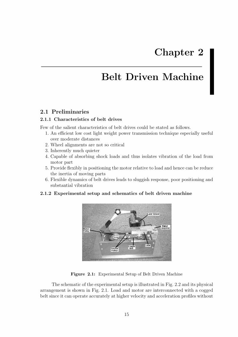
The schematic of the experimental setup is illustrated in Fig. 2.2 and its physicalarrangement is shown in Fig. 2.1. Load and motor are interconnected with a coggedbelt since it can operate accurately at higher velocity and acceleration profiles without
15

16 2. Belt Driven Machine
Cosmos
D/A
A/D
J1
J2
J3
24v DC+ -
+ G
0 V
Belt drive machine
Motor
Computer
Servo pack
Connector
Pulse counter
DC power supply
Stand
Amplifierunit
Sensor head
Figure 2.2: Schematic Diagram of Belt driven Machine
any relative slip. The servomotor is excited by an embodied servo controller throughresident PI control algorithm.
The reference input, in other words generated trajectory is compensated fordelay dynamics and vibrations prior to use it for servoing with the aid of COS-MOS, which interfaces digital data with analog servo input. COSMOS is equippedwith multi channel A/D and D/A converters, 16MB memory and a digital counter.COSMOS is not only acting as an interface, but also as a data logger to support fastservoing with a sampling time smaller as 125 µs. An optical laser sensor coupled withan amplification unit devised to monitor the actual position and these data are alsologged back to the computer used as reference input generator, through COSMOS.
2.2 Problem Statement and Planning Algorithm
2.2.1 Problem statement
Servo controllers undergo current saturation and this phenomenon corresponds toacceleration limits in velocity profiles. The planned trajectories should comply withthe acceleration bounds and it can be mathematically expressed as
|r(t)| ≤ rmax; ∀t, (2.1)
where r(t) and rmax denote the acceleration of trajectory to be planned and its max-imum limit.
Maximum permissible velocity of a joint can either be governed seldom by thehardware limitation of the motors or frequently by the specifications of the applicationitself. If the operation is limited by a velocity constraint within the entire operation,angular velocity should not exceed the maximum allowable value as constrained bythe application itself. If the operation is limited by a velocity constraint, within theentire operation, angular velocity should not exceed the maximum allowable value asconstrained by
|r(t)| ≤ rmax; ∀t, (2.2)
2.2. Problem Statement and Planning Algorithm 17
where r(t) and rmax represent the velocity at time t and the maximum velocity ofobjective trajectory respectively.
Besides, the vibration and oscillations persisted in the actual tracking profile ofbelt drives should be brought down to an acceptable level, though a limit for it doesnot consider quantitatively.
2.2.2 Trajectory planning algorithm and overview of compensation
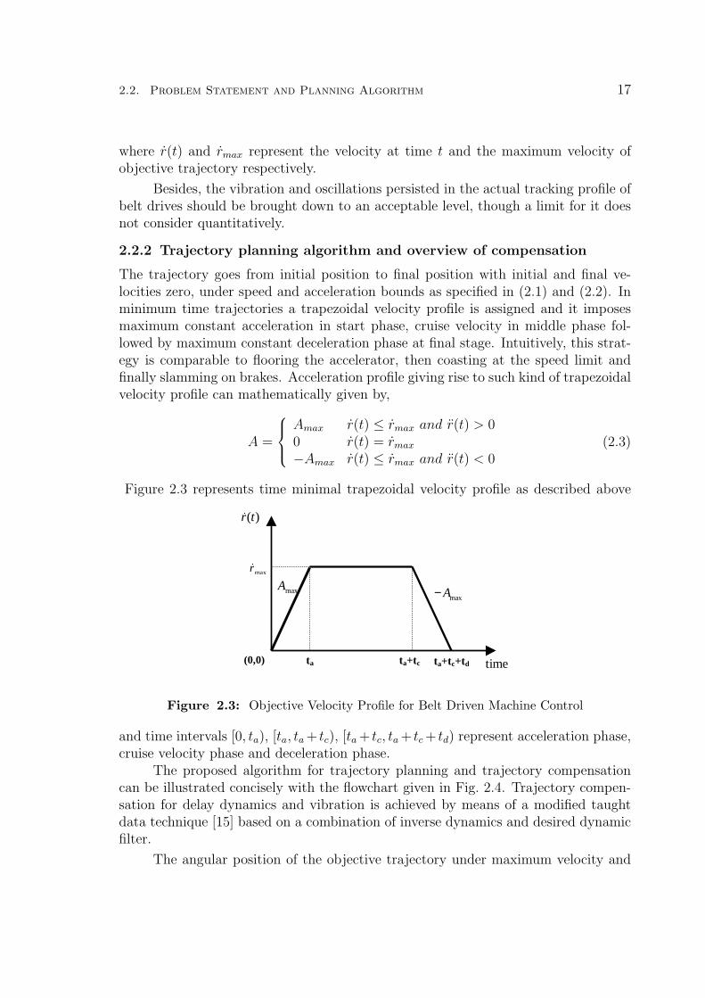
The trajectory goes from initial position to final position with initial and final ve-locities zero, under speed and acceleration bounds as specified in (2.1) and (2.2). Inminimum time trajectories a trapezoidal velocity profile is assigned and it imposesmaximum constant acceleration in start phase, cruise velocity in middle phase fol-lowed by maximum constant deceleration phase at final stage. Intuitively, this strat-egy is comparable to flooring the accelerator, then coasting at the speed limit andfinally slamming on brakes. Acceleration profile giving rise to such kind of trapezoidalvelocity profile can mathematically given by,
A =
Amax r(t) ≤ rmax and r(t) > 00 r(t) = rmax
−Amax r(t) ≤ rmax and r(t) < 0(2.3)
Figure 2.3 represents time minimal trapezoidal velocity profile as described above
)(tr
�
maxr�
ta ta+tc ta+tc+td time
maxAmaxA−
(0,0)
Figure 2.3: Objective Velocity Profile for Belt Driven Machine Control
and time intervals [0, ta), [ta, ta + tc), [ta + tc, ta + tc + td) represent acceleration phase,cruise velocity phase and deceleration phase.
The proposed algorithm for trajectory planning and trajectory compensationcan be illustrated concisely with the flowchart given in Fig. 2.4. Trajectory compen-sation for delay dynamics and vibration is achieved by means of a modified taughtdata technique [15] based on a combination of inverse dynamics and desired dynamicfilter.
The angular position of the objective trajectory under maximum velocity and

18 2. Belt Driven Machine
Objective point
Realizable trajectory (Maximum joint acceleration and maximum joint velocity strategies)
��
���
<−=>
=
���
=−+<−+−+=
0)()(0
0)()()()(2/)()()(
max
max
max
maxmax
max2
trifArtrif
trifAAwhere
rtrifttrrrtrifttAttrrtr
ii
iii
����
��������
Modified taught data
)(/)()( sGsHsF L= where 44 )()( γγ −= ssH
Input to the belt drive machine (command time interval 250[µs])
Realizable trajectory generation Sampling time 250[µs]
Taught data generation
Figure 2.4: Trajectory Generation Criterion for Trapezoidal Velocity Profile
maximum acceleration strategy is governed by
r(t) =
{ri + r(t− ti) + A(t− ti)
2 r(t) ≤ rmax
ri + rmax(t− ti) r(t) = rmax(2.4)
On the basis of the above formation, the trajectory-planning algorithm generatesa time sequence of joint variables that determines the motor position over time inrespect of the imposed constraints. Since the servo controller is of zero order hold,not all continuous timely positions are important but interspaced at sampling time.Therefore, the positions of joints are discretized in time domain with sampling timeT for servoing purposes and t takes the discrete values specified by
t = iT i = 1, 2, 3, ...N (2.5)
where NT is the total time of operation.
2.3 Spiky Phenomenon in Velocity Profile of Belt Drives
A significant spiky phenomenon in motor’s velocity profile is evident in the exper-imental results given in Fig. 2.5. However, well established first order and secondorder kinematic models of servo system are incapable of characterizing the spiky phe-nomenon in velocity profile. A non-trivial belt reaction torque gives rise to this spikyphenomenon in velocity profile. The gear ratio of motor to load is 1:1 and it affectsthe belt reaction torque of becoming significant in two senses,

2.4. Proposed Model and Solution Strategy for Belt Driven Machine 19
0.6 0.8 10
2
4
6
8
0.6 0.8 10
10
20
30
Time [s]
Experimental output of belt driven machine
Mot
or p
osit
ion
[rad
]A
ngul
ar v
eloc
ity
[rad
/s]
Figure 2.5: Spiky Phenomenon in Velocity Profile of Belt Driven Machine
1. No gear ratio scaling of the inertia torques of the load due to sudden change inacceleration
2. High-speed manipulation of the load associated with higher momentum andin turn, it creates high inertial load torques especially under minimum timeoperation, as the acceleration is rapid.
Significant reaction torque of the load definitely deviate the following trajectoryfrom objective trajectory and leads to poor tracking as well as inaccurate positioning.Flexible dynamics may further intensify the inaccuracies and therefore proper com-pensation technique with careful consideration of belt reaction becomes mandatory.
In the experiment, motor angle throughout the operation and the load angle inthe vicinity of final position were under investigation on the following grounds.
1. Motor angle encompasses the dynamics of the load and also much sensitive toservo dynamics. Therefore motor position based model validation is much moreeffective on the contrary to conventional approaches based on load position, asflexible dynamics assimilate sensitive dynamics.
2. Since the final positioning is of utmost importance in case of a position controlsystem, the limited sensor range of the accurate laser sensor was utilized toobtain the exact load position near the final position.
2.4 Proposed Model and Solution Strategy for Belt DrivenMachine
2.4.1 Rationale
Though the position accuracy is quite high in PID control, the tracking accuracy isoften rather poor, since there is no direct compensation for friction and inertial forces.

20 2. Belt Driven Machine
In addition, as flexible belt driven mechanism possesses flexible characteristics, systemhas two degrees of freedom but only one control input, the angular position of themotor. Therefore the input to the system should be compensated for flexible dynamicsand delay dynamics as PID controller inherently undergoes tracking error. However,sufficiently acceptable performance could be realized with belt drives even withoutdynamic compensation when they confined to very low speed operations. In orderto respond fast changing sequences of input trajectory with minimum tracking errorand restraint vibration, dynamic compensation is essential and crucial.
This is accomplished with a feed forward compensator based on the principleof concatenating the inverse dynamics of belt driven machine and desired dynamicfilter. As the key underlying objective of the proposed method is to deploy beltdrives in high-speed operations and thereby extend the bounds of application scope,encapsulation of belt reaction torque. The root cause for inaccuracies in inversedynamics part of the compensator is indispensable as pointed out in Chapter 2.3.
2.4.2 Model construction
Load reaction torque does not incorporate within the first and second order kine-matics models of servo systems and assumed to be negligible. However, this effectis non-trivial in high-speed belt drives due to 1:1 gear ratio and high-speed motion.Integration of belt reaction torque and consideration of flexible dynamics are the fun-damental concerns in the development of an accurate model for servo controlled beltdriven joints valid under high-speed operations.
The derivation of the model excogitating the flexible dynamics of belt drivesare carried out under following three most applicable and practical assumptions.
1. The inertia and the friction of tension pulleys are negligible,2. The mass of the belt is negligible and the belt has insignificant bending rigidity,
and,3. Belt drive operates within the linear elastic range of the belt.
The torques experienced by the motor pulley is the effective torque generated by themotor, motor initial torque, and the reaction torque of the belt. Under the torquesstated above, the motor pulley attains its equilibrium. The effective torque exertedby the servomotor is equal to the torque generated by the motor due to the servoingaction less the reaction torque due to back emf. Therefore, the effective motor torque,τM is given by,
τM = KpKgv (u− θM)−Kg
v θM (2.6)
where u, Kp, Kgv and θM represent the input to the servo system, the position loop
gain, the velocity gain of the servo amplifier and the position of the motor, respec-tively.
The inertia torque on the motor due to the mass of the rotational part of themotor and coupled pulley τI is expressed by τI = JM θM , where JM is the moment ofinertia of the rotor including the motor pulley. When the motor pulley rotates in thedirection indicated in Fig. 2.6, the upper belt segment increases its tension whereasthe lower segment reduces its tension by equal amount due to the differential angular

2.4. Proposed Model and Solution Strategy for Belt Driven Machine 21
T1 . T1
rp rp
Mθ .
Lθ .
MJ LJ
T2 . T2
Motor pulley
Load pulley
Figure 2.6: Flexible Structure of Belt Drive
motion of the motor pulley and load pulley. Hence the tangential effective force oneither pulley, T1 − T2 is equal to twice the change in belt tension owing to motion
T1 − T2 = 2kcrp(θM − θL) (2.7)
where kc, rp and θL represent the linear coefficient of belt drive elasticity, radius ofeither pulley and position of the load, respectively. Therefore the reaction torque ofthe belt on either pulley τR is described by
τR = KL(θM − θL) (2.8)
where KL represents the angular coefficient of elasticity of the belt. Considering theequilibrium of torques on the motor pulley, the governing relationship among theinput u, motor position θM and load position θL in Laplace domain can be expressedby
KpKgvU(s) = [JMs2 + Kg
vs + KpKgv + KL]θM(s)−KLθL(s) (2.9)
The load pulley is driven by the tension of the belt whereas the load experiencesviscous damping torque and inertia torque, under which it achieves equilibrium. Theequilibrium of the load pulley can be represented mathematically in s domain by
KLθM(s) = [JLs2 + DLs + KL]θL(s) (2.10)
where JL and DL are the load inertia and the viscous damping coefficient of the load,respectively. Combining the relationships stated in (2.9) and (2.10), it is possibleto derive the transfer functions GM(s) = θM(s)/U(s) and GL(s) = θL(s)/U(s) asfollows:
GM(s) =b2s
2 + b1s + b0
a4s4 + a3s3 + a2s2 + a1s + a0
(2.11)

22 2. Belt Driven Machine
b0 = KP KgvKL
b1 = KP KgvDL
b2 = KP KgvJL
a0 = KP KgvKL
a1 = KLKgv + KP Kg
vDL + KLDL
a2 = KLJM + DLKgv + KP Kg
vJL + KLJL
a3 = DLJM + KgvJL
a4 = JLJM
andGL(s) =
a0
a4s4 + a3s3 + a2s2 + a1s + a0
(2.12)
a0 = KpKgvKL
a1 = KLKgv + KpK
gvDL + KLDL
a2 = KLJM + DLKgv + KpK
gvJL + KLJL
a3 = DLJM + KgvJL
a4 = JLJM
Figure 2.7 concisely illustrates the derived in the form of block diagram and dynamics GM(s) GL(s)
MθLθu
PK gVK
sJM
1LK
LD
s
1
s
1sJ L
1
Belt reaction force
Servo system Flexible belt drive
-
- -
+ ++ + +
- -
Figure 2.7: Fourth Order Model of Belt Driven Machine
associated with servo motor part and flexible structure part indicates separately.
2.4.3 Modified taught data technique
Goto et al. [15] is the proponent of the modified taught data technique to improvethe tracking accuracy of the mechatronic servo system. Modified taught data tech-nique is a feed forward compensating strategy to scale or reform the characteristicsof planned trajectory well suited to the dynamic characteristics of the system and itsconcept is illustrated in Fig. 2.8. Every feed forward compensator is worked on theprinciple of pole assignment or pole zero cancellation in view of improving desireddynamics cum rejecting disturbances and always located at the extreme end of thetrajectory planner. Since the taught data modifier, the dynamic compensator can

2.4. Proposed Model and Solution Strategy for Belt Driven Machine 23
)(sF
)(sGL
Servo controller and flexible structure
Modified data U(s)
Raw input trajectory R(s)
Feed forward dynamic compensator
Output load position θθθθL(s)
Figure 2.8: Concept of Modified Taught Data Technique
conveniently implemented inside the reference input generator neither any change tohardware setup nor a considerable reconfiguration of the system; this technique isreadily welcome by the industry.
2.4.4 Design of Feed Forward Compensator
A detailed analysis of feed forward compensator F (s) in Fig. 2.8 is furnished here.Proper selection of dynamic compensator can not only compensate delay dynamics,but also restrain vibration of the system of flexible structures. In general, selection offeed forward dynamic compensator is an objective selection and many methodologiesprovide different options. A combination of inverse dynamics and desired dynamicfilter constitutes the proposed compensator as depicted in Fig. 2.9.
)(1 sGL−
)(sH
Inverse dynamics
Desired dynamic filter
Modified data U(s)
Raw input trajectory R(s)
Feed forward dynamic compensator F(s)
Figure 2.9: Dynamic Compensator for Data Modification
Dynamics of the feed forward compensator can be explained by
F (s) =H(s)
GL(s)(2.13)
where H(s) is the desirable dynamic filter, whose dynamics is characterized by
H(s) =γ4
(s− γ)4(2.14)
where γ is the location of four coincident poles.
The exact cancellation of the system dynamics with the inverse dynamics com-ponent of the feed-forward compensator eventually gives rise to attainment of outputtrajectory R(s)H(s), which is a dynamic filtered version of the objective trajectory.

24 2. Belt Driven Machine
The characteristics of the desired dynamic filter are directly attributed in the realizedtrajectory. Therefore, the desired dynamic filter, H(s) should be constituted to im-part desired dynamic features such as oscillation free response with optimum settlingtime.
The numerator of 1/GL(s) is a fourth order polynomial whereas the denominatoris of zeroth order. Therefore, four zeros and no poles are introduced to the transferfunction H(s)/GL(s) due to inverse dynamic component 1/GL(s). As the inversedynamic component of the feed-forward compensator has four zeros, the fourth orhigher order dynamic filter, H(s) should be implemented to diminish the effect ofthe differentiation operation in dynamic compensation. Failure in integrating suchpartial design of the dynamic filter into the dynamic compensator would result in theappearance of very fast sequences seriously leading to torque saturation of the motorand ultimately obstructing smooth functioning of the system. Reduction in samplingtime is a favorable phenomenon to support smooth and vibration free controlling ofthe belt driven system, however, it itself adversely fetters the smooth performance ininstances where there is poor design in the dynamic filter.
Locating the poles of dynamic filter (γ) on the negative real axis causes to realizeoscillation free response whereas the coincident of poles optimizes the settling time.By locating the poles, γ further away from the imaginary axis dynamic response canbe made fast but increasing the magnitude of the poles unnecessarily will result ingenerating fast sequences in time domain for servoing subsequently affects for thecurrent saturation of servo amplifier and thus deteriorates the overall performance.However in general, there is no way to know a priory the best pole location [16].
2.4.5 Analytical solutions
As an alternative and much realistic technique for numerical simulation based on re-cursive iteration (accumulation of numerical error over iteration leads to non-convergentresults and impair the accuracy dramatically) system dynamics was analyticallysolved for the taught data input and obtained the exact solutions for the joint positionto conform the numerical robustness of simulation.
The reference input u(t), used for servoing is a time-based input with zeroorder hold sequence having variable marginal magnitudes. It can be decomposed intoa summation of time-shifted step input series with variable step size. Therefore, themodified taught data can be written as:
u(t) =k∑
i=1
∆u(iT )w[(k − i)T ] (2.15)
where ∆u(iT ) = u(iT )− u((i− 1)T ), kT ≤ t ≤ (k + 1)T , T is the sampling time andw is the unit step function. If the system is excited with u(t), motor angular positionθM(t) and the load position coordinates θL(s) could be expressed with
θM(t) =k∑
i=1
∆u(iT ){1 + A1e−α1(t−iT ) + A2e
−α2(t−iT ) (2.16)

2.4. Proposed Model and Solution Strategy for Belt Driven Machine 25
+A3e−ξωL(t−iT )sin(ωL
√1− ξ2(t− iT ) + φ1}
where kT ≤ t ≤ (k + 1)T and
g1 = a3/4a4
g2 = (2a32 − 9a1a2a3 + 27a0a
23 + 27a2
1a4 − 72a0a2a4)2
l =√−4(a2
2 − 3a1a3 + 12a0a4)3 + g2
m = 2a32 − 9a1a2a3 + 27a0a
23 + 27a2
1a4 − 72a0a2a4
c = 3
√(m + l)
n = 3√
2(a22 − 3a1a3 + 12a0a4)/3a4c
p1 =
√a23
4a24− 2a2
3a4+ n + c
3√23a4
p2 = −a33
a34
+ 4a2a3
a24− 8a1
a4
q1 =
√a23
2a24− 2a2
3a4− n− c
3√23a4− p2
4p1
q2 =
√a23
2a24− 2a2
3a4− n− c
3√23a4+ p2
4p1
α1 = −g1 − 0.5p1 − 0.5q1
α2 = −g1 − 0.5p1 + 0.5q1
ωL =√
g21 − g1p1 + 0.25(g2
1 + q22)
ξ = (g1−0.5p1)√g21−g1p1+0.25(g2
1+q22)
A1 = b2α1+b1α1+b0(α1−α2)(α2
1+2ξωLα1+ωL)
B2 = b2α2+b1α2+b0(α2−α1)(α2
2+2ξωLα2+ωL)
C = −(A1 + A2)D = b0
α1α2+ (A1
α1+ A2
α2)ω2
L
B3 =√
E2 + (L−EξωL)2
ω2L
φ1 = tan−1{C√
1−ξ2ωL
(D−CξωL)}
and
θL(t) =k∑
i=1
∆u(iT ){1 + B1e−α1(t−iT ) + B2e
−α2(t−iT ) (2.17)
+B3e−ξωL(t−iT )sin(ωL
√1− ξ2(t− iT ) + φ2}
where kT ≤ t ≤ (k + 1)T and
B1 = a0
(α1−α2)(α21+2ξωLα1+ωL)
B2 = a0
(α2−α1)(α22+2ξωLα2+ωL)
E = −(B1 + B2)L = α0
α1α2+ (B1
α1+ B2
α2)ω2
L
B3 =√
E2 + (L−EξωL)2
ω2L
φ2 = tan−1{E√
1−ξ2ωL
(L−EξωL)}

26 2. Belt Driven Machine
Table 2.1: Parameter Values of Belt Driven Machine
Description of parameter Symbol Value Position loop gain pK 15 [1/s]
Servo amplifier velocity gain constant gvK 0.0023[kgm2/s]
Angular spring constant of belt LK 0.0513[kN/rad] Viscous damping coefficient of load LD 5.24X10⁻⁴[Ns/rad] Location of poles γ -130 Maximum velocity maxr
�
24[rad/s] Maximum acceleration maxr
��
4314[rad/s2]
2.5 Performance and Evaluation
The trajectory is generated with proposed planner, subsequently compensated forflexible dynamics and then used for real time servoing of actual belt driven machine.Further, a simulation study has been carried using conventional numerical techniquesand also proved the validity of it using the analytical solutions derived. The param-eters used for trajectory generation and simulation could be given in the Table.2.1
0.6 0.8 10
2
4
6
8
0.6 0.8 10
10
20
30
0.6 0.8 1-3000
-1500
0
1500
3000
0.6 0.8 10
2
4
6
8
Inpu
t u [
rad]
Mot
or p
ositi
on θ
M [
rad]
Vel
ocity
θM
[r
ad/s
]
Acc
eler
atio
n θ M
[r
ad/s
2 ]
SimulationNumerical Analytical
0.6 0.8 10
2
4
6
8Experiment
0.6 0.8 10
2
4
6
8
0.6 0.8 10
10
20
30
0.6 0.8 1-3000
-1500
0
1500
30000.6 0.8 10
10
20
30
0.6 0.8 1-3000
-1500
0
1500
3000
Time [sec]Time [sec] Time [sec]
0.6 0.8 10
2
4
6
8
0.6 0.8 10
2
4
6
8
Figure 2.10: Simulation and Experiment Results of Belt Driven Machine
Figure 2.10 shows the results obtained for motor position by experiment as well

2.6. Concluding Remarks 27
as simulation based on analytical solutions and recursive techniques. By numericaldifferentiation corresponding velocities and acceleration were derived. In order toeliminate noises in the acceleration profile of the experiment, acceleration data isobtained by filtering the original data with a fourth order Chebyshev IIR low passfilter of 100Hz.
A significant spike could be noticed in the motor velocity profile of the proposedmodel at the times of changing the acceleration and it is expectable with belt reactiontorque, as sudden changes in load acceleration has the consequences of rapid changein load inertia torque. The magnitude of the spike, the quantification aspect of themotor velocity spike of the proposed model is almost in accordance with the resultsobtained in experiment and hence proven the validity of the model.
Mathematically, the presence of two zeros in the transfer function (in equation(2.11)) causes the linear combination of first and second derivatives of the input todirectly contribute to generate the output giving rise to higher sensitivity to inputdynamics. Therefore, zeros in the transfer function assist to represent input dynamicsdominantly, especially in the instance of a sudden change in acceleration profile witha spike in velocity profile.
0.9 1.05 1.2
-0.4
-0.2
0
0.9 1.05 1.2
-0.4
-0.2
0
Posi
tion
erro
r [r
ad]
Time [s] Time [s]
Experiment Simulation
Figure 2.11: Comparison of Load Position Error
A comparison of the load position error profiles are provided in Fig. 2.11 andhere load position error is defined as the final desired position subtracted from thecurrent position of the load. The experimental load position error in Fig. 2.11 con-taminated with noises due to quantization error of the data acquisition and noise ofthe laser sensor. No oscillations could be observed in load positioning and thereby theachievement of the vibration restraint with the proposed method has been verified.
The final objective, accurate positioning of the load has been investigated withload position error. However, the sensor range is limited to the vicinity of the finalposition and hence the experiment results may not be permitted to cover the entiretracking. For the sake of completeness, simulation results of the load position arefurnished in Fig. 2.12.
2.6 Concluding Remarks
Numerous applications of position control devices based on servo driven belt drives areubiquitous in industry. Belt drives are effectively employed as a power transmission

28 2. Belt Driven Machine
0.6 0.8 1
-1000
0
1000
Loa
d P
ositi
on θ
L [
rad]
Vel
ocity
θL[r
ad/s
]A
ccel
erat
ion
θ L[r
ad/s
2 ]
Time [s]
0.6 0.8 10
2
4
6
8
0.6 0.8 10
10
20
30
Figure 2.12: Simulation Results of Load Tracking
technique in light weight robots as belt drives enable to reduce the inertia of the robotarm through mounting the servo motors on stationary base. Linear positioning tableis another dominant application of belt drives in industry.
Development of an accurate model representing precise dynamics of flexible beltdrives, planning of trajectory under maximum acceleration and velocity constraints,designing of a feed forward compensator to compensate flexible dynamics and re-straint vibration are basically covered in this chapter. There is a close similarityexist between the derived model for belt drives and the forth order kinematic modelfor robotic systems given in [70]. The modified taught data method, on which theproposed dynamic compensation is basically developed, has a quite good robustnessand hence the proposed control method also inherits robustness characteristics overservo parameter changes. Further, avoidance of oscillations and restraint of vibrationwould be another key advantageous properties inherited from modified taught datatechnique, due to proper selection of desired dynamic filter.
Considering the practical perspectives, elimination of vibration and oscillationsfundamentally contributed to speed up the operation by diminishing inter-operationsettling time and deterioration of product quality due to frictional effects under vibra-tions especially in wafer transfer applications. In addition proposed technique allowshigh-speed operation intact with the accuracy of positioning and thereby improve theproductivity through contracted cycle time. Using an off-line algorithm to plan thetrajectory and associated compensation, the proposed method has strong industrialimplications since it can be directly applied to existing belt driven servo systems

2.6. Concluding Remarks 29
without any hardware change.
Figure 2.13: Multi-axis Belt Driven Manipulator
Figure 2.13 illustrates a typical multi-axis lightweight robot manipulator equippedwith belt drives. The proposed control technique can be easily and conveniently ex-tended to control such multi-axis multi-dimension robot systems with decoupled ser-voing of each joint. However, change in load inertia with configuration is formidableparticularly under high-speed operation of robots. As the load to motor inertia mis-match increases, the system is heavily vulnerable for oscillations with increased set-tling time as a result of changed in natural frequency of the system, in addition to thepower loss due to inertia mismatch [71]. Additional power dissipation dramaticallyincreases as the mismatch gradually increases. These are few of open issues availablefor further investigation in multi axis belt driven robot system.

Chapter 3
Dual Arm Trajectory Planningfor a Specified Cooperative
Trajectory3.1 Cooperative Control
3.1.1 Definition and categorization of cooperative control
Cooperative control is defined as the controlling of multiple dynamic entities thatshare a common though perhaps not singular objective [72]. Cao et al. [73] de-fined the cooperative control as given some task specified by a designer, a multiplerobot system displays cooperative behavior if due to some underlying mechanism (i.e.mechanism of cooperation) there is an increase in total utility of the system. In bothdefinitions, integration of individual robot motions directs towards the accomplish-ment of a specified cooperative task or tasks under cooperative control.
The core concept of cooperative control encapsulates two issues: pure cooper-ation where the collaboration of system entities through communication, and purecoordination where collaboration is achieved through a set of complementary ruleswithout the benefit of communication [74]. It has been practically shown that a com-bination of these two concepts is more effective to optimize the time and the spatialefficiency. The following statement poses the importance of proper coordination fora cooperative task, and pure cooperation does not establish a sufficient support toachieve higher operational efficiency.“A human being using two arms has a greater advantage over two human beings, eachusing one hand.”
The fundamental motives of cooperative control can be stated as [75]:1. To increase the scope of mission inherently distributed in space, time and func-
tionality2. To increase the reliability and robustness through redundancy3. To decrease the task completion time through parallelism4. To increase the bounds of payload through parallelism5. To reduce the cost through much simpler individual robot design
According to the way of realization, cooperative control strategies are basicallyof two types [47]. They are:a) Loose cooperation
The manipulation task is executed by controlling the two robots in an indepen-dent fashion, so that cooperative operation is realized only at task planning level.Therefore, the approach is simpler, could be off-line, can operate without any
30

3.1. Cooperative Control 31
sensory feedback and the operation is pretty good in structured environments.b) Tight cooperation
The cooperation is realized not only at planning stage, but also at the controllevel. This can operate even under unstructured environment with a very littleprior knowledge, since sensory feedback could guide the task at the operationallevel.
The following mechanisms can be found in the literature as the solution strate-gies to cooperative control.i) Master-slave configuration:
Here the coordination of two robots is achieved through a force measurement.Further, independent controllers are implemented for operation. Therefore, it isconvenient in implementation point of view. This mechanism is also applicableto improve the end effector accuracy through cooperative control. A considerablediscrepancy of the capabilities of two robots may lead to a remarkable delay andin turn, it may have the danger of degrading the fidelity of master-slave systems.
ii) Hybrid position control:when all the robots are considered to be an unique entity, the degrees of freedomof the total system proportionally increases with the number of robots. A unifiedrobot approach may be assumed, and an object dynamic model was developed[52]. Motion and force control problem of multiple robots manipulating a coop-eratively held common object is basically addressed under this mechanism.
Distributed impedance control strategy technique can be applied to above bothsolution strategies [76] in which an independent controller controls each robot. Forceand position control actions are suitably dispatched to achieve both internal loadingcontrol and object position control.
3.1.2 Cooperative control research directions
Researches related to cooperative control were addressed in several research direc-tions and found in number of research domains including cooperative control ofmobile robots [73][77], dual robot coordinative control [67][69][78], and multirobotcollaboration [79][80][81] for single or multiple goals. Multirobot collaboration formanipulating a commonly held object is addressed by many researchers [82][79] andpopularly referred to as cooperative control. Dual arm cooperative control is inten-sively investigated for accuracy [83], vibration control [83], obstacle avoidance [84]and on many other aspects [85]. Further theoretical foundations have been developedfor cooperative handling of objects [64][65].
A number of sophistications has been realized in multirobot systems with theaid of sensory implementation, as sensory feedback can make them much responsive,flexible, efficient and robust. Therefore, sensory driven control schemes become im-perative for successful deployment of robots in most variety of tasks, particularly forcooperative tasks. However, inter-robot communication overhead and computationalcomplexity due to additional sensory signal processing becomes key factors as well asimplementation issues.

32 3. Dual Arm Trajectory Planning for a Specified Cooperative Trajectory
A fair amount of work has been directed towards the multirobot or dual robotmanipulation of commonly held object or accomplishment of decomposed coopera-tive sub-tasks by individual robots. However, the accent on cooperative trajectoryplanning under strict coordination and fully integrated cooperation is rather weak.Additionally, speed up of the cooperative task through coupled cooperative planningstrategies has not been exploited adequately.
3.1.3 Concept of cooperative control
The relative motion between the work piece and the tool constitutes a contour controlmotion in industrial applications. This is generally realized by keeping the work piecestationary and giving the required motion to the tool, which is usually held by the endeffector of a robot. It is also possible to give simultaneous complementary conjugatemovements to both work piece and tool such that the relative motion between thetwo shall be the objective contour. Such motion is called cooperative motion in thiscontext and it could be definitely used to increase the speed of operation and thus toreduce cycle time, eventually the task completion time.
A
B
Ax
Ay
Bx
By
inY
inX
Figure 3.1: Concept of Cooperative Control
Figure 3.1 illustrates the concept of cooperative control with a simple examplewhere tool A and work piece B represent a pen and a paper respectively. The motionsgiven to pen and paper in X and Y directions are denoted by [xA, yA]T and [xB, yB]T .The relative motion between the paper and pen [X in, Y in]T is the plotted shape onthe paper refering to a fixed point on the paper.
In cooperative control of robots, the cooperative locus should be decomposedinto complementary loci under dynamic and kinematic limitations. When a timeoptimal criterion is considered, it is not convenient to decompose the objective locusinto conjugate loci (loci of A and B) and thereby plan the robot trajectories for eachconjugate loci.

3.2. Preliminaries 33
3.2 Preliminaries
3.2.1 System overview
Ax
By Ay
Bx
Al2
Al3
Bl2
Bl3
Figure 3.2: Experiment Setup Illustrating Two-Robot Manipulator Configuration
Figure 3.2 gives a comprehensive illustration of the orientation of two indus-trial manipulators, Performer MK2 and MK3, alone with the selection of coordinateaxes. [αA, βA]T and [αB, βB]T denote the joint coordinate vectors of robot A and Brespectively. Similarly, [lA2 , lA3 ]T and [lB2 , lB3 ]T represent the link length vectors of thetwo robots. Joint 1 of robot A from the base is selected as the origin of the commoncoordinate system referred to as “the global coordinate system”. Two Cartesian coor-dinate systems are defined referring to robots A and B for convenient transformationof configuration space to working space and vise versa. As depicted in Fig. 3.2 the endeffector positions in space are described with respect to these two coordinate systemsas xA − yA and xB − yB referring to each robot.
3.2.2 Coordinate transformation
Kinematic and inverse kinematic transformations establish the relationship betweenthe configuration space and the working space. Initial locations of end effectors inspace determine the relative positions and their relationship established referring tothe global coordinate system. The coordinate system transformation among the threeCartesian coordinate systems described above is a one-to-one relationship.
[XA XB
Y A Y B
]=
[xA −xB
yA yB
] [0 XBO
0 0
](3.1)
where [XA, Y A]T and [XB, Y B]T give the spatial representation of end effectorsof the two robots referring to the global coordinate system. (0, 0) and (XBO, 0) arethe origins of the two Cartesian coordinate systems, xA − yA and xB − yB, referringto the global coordinate systems.

34 3. Dual Arm Trajectory Planning for a Specified Cooperative Trajectory
The cooperative trajectory [X in, Y in] can be expressed by
[X in
Y in
]=
[xA
yA
]−
[−xB
yB
](3.2)
The relationship between the cooperative velocity vc and cooperative acceleration ac
could be represented with the equations given by
vc =√
(X in)2 + (Y in)2 (3.3)
andac =
√(X in)2 + (Y in)2 (3.4)
3.2.3 Significance of piecewise linear off-line trajectory planning
With the advent of digital electronics and microprocessor based electronics, digitalcontrollers have identified as concise and precise means of controlling due to inherentflexibility ascribed by programmability. To cope with the digital world, discretizationof analog signal in time domain is essential and that permits to apply convenientplanning and simulation techniques. The time interval in which a digital controllertakes an action is referred to as update rate and it may vary from 0.1 to 100msdepending on the robot controller and the application.
Further, consideration of entire path for trajectory planning is rather compli-cated and it is much sensible to break the path into segments, each of which could behandled by the trajectory planner easily particularly in cooperative trajectory plan-ning. In the case of piecewise linear path, end effector would have to reduce the speedsignificantly at end points of each segment because it could not change the directionof velocity vector instantaneously. Therefore, consideration of perfect continuity, suc-cessive differentiability of trajectories at the merging points of such segments is ofprime importance for high-speed operations since imperfections may lead to consid-erably deteriorate the trajectory being followed and to generate nontrivial jerks whichwould be resulted in shortening the life span of the robots. Blending line segmentsof the path by quadratic arcs and use of spline techniques are accepted techniques toachieve continuity at merging points.
Besides, off-line trajectory planning and on-line trajectory tracking are generallyin industrial practice. However on-line trajectory planners are not readily welcomeby the industry on the following grounds.
1. On line trajectory planners are relatively complex and demanding for superpower reference input generators,
2. Proabability of risk and troublesomeness is quite high as compared to off-lineplanners and can not be conveniently implemented,
3. Most of the industrial tasks are carried out in structured environments andpossible disturbances are a priori known. Hence the trajectory planning can becompletely manageable with off-line planners,
4. Specifically, planning of accurate cooperative contours are highly computationintensive and therefore, on-line planning is not feasible under relatively higher

3.3. Problem Statement 35
updating rates. Therefore, off-line planning becomes indispensable in coopera-tive trajectory planning.
3.3 Problem Statement
The relative motion between the end effectors of two robots generates the cooperativetrajectory, when the two manipulators described in Chapter 3.2.1 are maneuveredsimultaneously. Therefore the cooperative trajectory should be resolved into twoconjugate trajectories such that the relative trajectory between them exactly givesthe cooperative trajectory.
Specifications of the path and the accuracy requirement referring to industrialtasks are generally expressed in working space. Besides, cooperative trajectory kine-matic specification such as maximum cooperative speed is determined by the appli-cation itself. Under bounded cooperative speed, cooperative velocity profile shouldbe of trapezoidal shape for a minimum time realization of cooperative task. In suchtrajectory, upper bound of the cooperative velocity can be specified by
|vc| = vclim ∀t (3.5)
where vclim is the maximum limit of cooperative velocity.
However, it is not pragmatic to realize the maximum cooperative velocity inzero time, and hence the maximum cooperative velocity should be reached underpractically viable cooperative acceleration. This cooperative acceleration constraintcan be mathematically expressed as
|ac| = aclim ∀t (3.6)
where aclim is the upper limit of cooperative acceleration.
The cooperative velocity profile and the objective locus are completely knownas per the specification of the application and hence the cooperative trajectory, therelative motion between two end effectors is a specified priori.
Motion of robot arms are originated by the servomotors connected to the jointsand hence the control action should be expressed in joint space. In most practicalconsequences, the maximum end effector velocity imposed by the application is notlimited by the joint velocity limits of the servo motors even in the single robot case[29] and therefore the joint velocity limit governed by the hardware limitations isbeyond consideration. However, the torque constraint imposed by hardware referringto the power amplifier current rating, inflicts a joint acceleration limit. In cooperativecontrol of two robot arms, no joint of any robot can exceed the joint acceleration limit.Thus the bounded joint acceleration can be stated as
|αA(t)| ≤ (αA)lim
|βA(t)| ≤ (βA)lim
|αB(t)| ≤ (αB)lim
|βB(t)| ≤ (βB)lim
(3.7)

36 3. Dual Arm Trajectory Planning for a Specified Cooperative Trajectory
where [αA(t), βA(t), αB(t), βB(t)]T and [(αA)lim, (βA)lim, (αB)lim, (βB)lim]T denote theacceleration of the joints of two robots at time t and the limits of the acceleration ofcorresponding joints respectively.
3.4 Two Stage Trajectory-Planning Paradigm
3.4.1 Rationale
The planar example of cooperative control used to illustrate the concept of coopera-tive trajectory planning has four degrees of freedom (two joints contributed from eachrobot) to achieve two-dimensional cooperative spatial position and hence two-degreesof freedom are redundant. The redundant two degrees of freedom (DOF) give rise togenerate many solutions when the cooperative position at the end of linear segmentis solved for joint space vectors of each robot. As the piecewise linear trajectory isrealized through sequential planning of linear line segments, the solution space growsexponentially in the form of a tree. Number of branches originated from a particularnode is governed by the number of multiple solutions generated at that node and inturn the trajectory generation becomes computationally hard and numerically infea-sible at high resolution approaches. Granularity of solutions determines the widthof the solution space tree and the size of the segment or time used for segmenta-tion determines the depth. A trade off exists between the accuracy of the generatedtrajectories and the computational complexity.
The key concept of cooperative trajectory generation is the decomposition ofthe cooperative task into complementary subtasks. Having completely specified thecooperative trajectory (time history of countering locus) based on application, thereis no provision to optimize the operational time but to optimize the performancecharacteristics of each robot. An even task decomposition between two robots isselected as the criterion to optimize and defined an objective function Z such that
Max{Z} = {|max{|αA|, |βA|} −max{|αB|, |βB|}|}. (3.8)
When optimizing the objective function Z, by bringing the maximum joint velocitiesof each robot as closer as possible, an excessive movement of either robot is minimized.
To facilitate the optimization criterion, a search algorithm should be devisedover the solution space. However, yielding no solution for a particular planning seg-ment give rise to terminate the propagation of solution tree structure at that node.The harder the acceleration constraint is, the higher the number of such termina-tions in propagation (branching to the next level) as well as the tree becomes leanin breadth wise. However the prediction of termination in branching can not be de-termined in advance through a look-ahead approach due to the nonlinearities of thespace transformation. Nevertheless, a proper directive scheme can successfully guidefor a breadth wise reduction of the state tree as well as to avert the terminationof branching and thereby leading for a promising results within a remarkably lowercomputational time. Further, reduction in the number of segments compromising theaccuracy of the contour followed can also be shrinked the depth of the tree. Theseprovisions in scaling down the size of the solution space (reduce the number of nodes

3.4. Two Stage Trajectory-Planning Paradigm 37
in state tree structure) enable to realize the solutions, even though the algorithm isNP hard.
3.4.2 Realization of cooperative control
inAx
inAy
inBx
inBy in
Bβ
inBα
inAβ
inAα out
Aα
outAβ
outBα
outBβ
outAx
outAy
outBx
outBy
Xin
Yin Yout
Xout
n
Fun
ctio
n F
Inve
rse
Kin
emat
ics
Inve
rse
Kin
emat
ics
Kin
emat
ics
Kin
emat
ics
Fun
ctio
n F
-1
Dynamics G(s)
Dynamics G(s)
Dynamics G(s)
Dynamics G(s)
Robot A
Robot B
Figure 3.3: Realization of Cooperative Control
The strategy used in the realization of cooperative control is illustrated inFig. 3.3. Initially, the cooperative locus is transformed into the cooperative trajectoryconsidering the application-oriented specifications such as the maximum cooperativespeed and some pragmatic concerns like cooperative acceleration. The input cooper-ative trajectory [X in, Y in]T specified in the Cartesian coordinates is decomposed intotwo Cartesian time sequences for robot A and robot B using the Cartesian trajectorydecomposing function F . The generated complementary trajectories of robots A andB in Cartesian space are denoted by xin
A , yinA and xin
B , yinB respectively. The correspond-
ing joint space transformations are given by [αinA , βin
A ]T and [αinB , βin
B ]T . [αoutA , βout
A ]T
and [αoutB , βout
B ]T represent the output positions obtained under dynamics G(s). Subse-quently kinematic transformation is applied to convert them into working coordinates[xout
A , youtA ]T and [xout
B , youtB ]T . The relative motion between the end effectors specified
in Cartesian coordinate constitutes the output cooperative trajectory [Xout, Y out]T inCartesian space. The well-known second order linear kinematics model, G(s) is usedfor simulation and it can be represented by
G(s) =KpKv
s2 + Kvs + KpKv
(3.9)
where Kp and Kv are position and velocity loop gains of the servo system.
The Cartesian trajectory decomposition function F is more than a mathematicalrelationship due to imposed optimization criterion and the necessity to foresee thedynamic capabilities of each robot specified in joint space. An algorithm is developedto attain the function F and focuses the attention on it.

38 3. Dual Arm Trajectory Planning for a Specified Cooperative Trajectory
3.4.3 Trajectory generation criterion
i) Selection of segmentation time:At first, the objective trajectory is segmented based on a time interval T suchthat the end of one segment is the starting point of the next segment. The timeused for segmentation of the objective locus is termed as segmentation time andit is essentially an integer multiple of sampling time. As start and end pointsof each segment become the path points, the tracking profile is improved withlower segmentation time. However, a compromise between the accuracy andthe computational overhead in trajectory planning determines the segmentationtime.
ii) Generation of the global solution space and state tree:Planning of complementary trajectories is carried out piecewise manner at seg-ment level and sequentially to cover the entire cooperative trajectory. However,motion planning of two robots at each segment produces the feasible solutionspace comprising multiple solution candidates, and collection of such feasiblesolution candidates subsequently form the global solution space. The global so-lution space can be graphically represented in the form of a tree and it is referredto as state tree.
Segment 1
Segment 0
(i) Selection of optimum node
Segment 1
Segment 2
Segment 0
(ii) Generation of children
Segment 1
Segment 3
Segment 2
Segment 4
Segment 0
(iii) Successive deletion of nodes
Segment 1
Segment 3
Segment 2
Segment 4
Segment 0
(iv) Successive generation of childrenfrom the best available nodes
Figure 3.4: State Tree of Global Solution Space
Synopsis of the fundamental steps in developing the state tree is depicted inFig. 3.4 and they can be stated as

3.4. Two Stage Trajectory-Planning Paradigm 39
a) Searching for optimum nodeBased on the value of the objective function, the optimum node is optedamong available nodes at a certain level of the state tree. The selectedoptimum node is shaded with a light grey in Fig. 3.4-(i).
b) Generation of children at optimum nodeGeneration of children is allowed only for the optimum node. Transitionfrom one node to another node in next level indicates the advancement oftrajectory planning through successive segments. The refined solution spacewould rather be used in the construction of state tree by appending therefined solutions to span the global solution space as referred in Fig. 3.4-(ii).
c) Successive deletion of nodes in absence of optimal nodesThe occurrence of no solution at the optimal node at a particular segment ofthe cooperative trajectory causes to delete that node and search the secondoptimal node at the same level. In case of failure to find such node compelsto fold back one level up (move to parent level) in the tree-structured globalsolution space. The corresponding node at the parent level is also deleted insearch of next optimal node for ensuing branching. Successive occurrence ofthis scenario is depicted in Fig. 3.4-(iii). The deleted nodes are representedwith dotted circles whereas the discarded transition to these nodes is denotedwith dotted arrows.
d) Successive generation of children from the best available nodesFig. 3.4-(iv) elucidates the successive generation of children for the best avail-able optimal node without termination of spanning or without experiencingthe occurrence of no solution condition.
iii) Two stage trajectory planning:For servoing purpose, the time separation of trajectory should be at samplingtime but the planning horizon for each segment can not be made to that scalebecause planning of the cooperative trajectory becomes exceedingly computa-tion intensive. Therefore, planning of two complementary trajectories is realizedat two modular stages, coarse level (knot level) or segment level planning (referChapter 3.4.4 for details) and fine level refinement. The refinement of plan-ning trajectories is carried out with an optimized interpolation scheme (detailsprovided in Chapter 3.4.7) concerning the errors incorporated. This two-stagetrajectory planning paradigm is equipped with short-listing criterion describedin Chapter 3.4.5, to manage the complexity of calculation.
iv) Algorithm of trajectory planning:The overall algorithm encompassing two stage trajectory planning can be eluci-dated with the steps stipulated below.1. Generation of feasible solutions for a segment (generate feasible solution
space)2. Filter-out the feasible solution space for more probable candidate solutions
using short-listing criterion (extraction of the refined solution space)3. Span the state tree using the refined solution space4. Selection of optimal node based on the value of the objective function

40 3. Dual Arm Trajectory Planning for a Specified Cooperative Trajectory
5. Repeat the above steps 1)∼4) until encountering no solution for a particularsegment or covering all the segments of the objective trajectory
6. If no solution exists, delete the node in search of next optimum node amongthe available nodes at the same level of state tree repeatedly. In case of nosuch node available, recursively move to the parent level deleting the node,from which the last generation of children have been produced
7. Above steps 1)∼6) have to be reiterated until the completion of the entirecooperative trajectory. The solutions that cover the entire cooperative tra-jectory in segment wise, constitute the conjugate trajectories for robot Aand B
8. Interpolation of joint positions for inter-segmentation time using fourth or-der, minimum acceleration interpolation scheme
The proposed trajectory-planning algorithm in its entirety can be precisely rep-resented by the flow chart given in Fig. 3.5. This algorithm is capable of yieldingcomplementary trajectories of cooperative robots within acceptable time duration,while optimizing the distribution of the cooperative task between two robots. Themathematical notion of the algorithm will be discussed in Chapters 3.4.4, 3.4.5and 3.4.7.
3.4.4 Segment Level Trajectory Planning
The algorithm responsible for the generation of feasible solution, depicted by theblock in between P and Q in Fig. 3.5, is explained in detail under this section. Thedetailed block diagram for feasible solution generation is illustrated by Fig. 3.6.
The relevant mathematical calculations of generating the feasible solution spacefor a particular segment of the cooperative trajectory are illustrated in the form ofequations. Initially, joint velocities of robot A are selected as independent parametersto generate solutions according to
[αA(ti)
βA(ti)
]=
[αA(ti−1)
βA(ti−1)
]+
[(αA)maxk1
(βA)maxk2
]T (3.10)
where k1 and k2 are parameters within the interval [-1,1]. The complete continuumof joint velocities, which conforms the acceptable parameter values is beyond con-sideration, and hence a discrete set of equi-spaced joint velocities with an adequateresolution is selected. The next joint position is evaluated for each joint velocity usingthe Euler formula given by
[αA(ti+1)βA(ti+1)
]=
[αA(ti)βA(ti)
]+
[αA(ti)
βA(ti)
]T (3.11)
where T is the time interval used to segment the cooperative trajectory or segmenta-tion time. The kinematic equations transform set of solutions in joint space into onein the working space as
[xA(ti+1)yA(ti+1)
]=
[sin[αA(ti+1)] sin[αA(ti+1) + βA(ti+1)]cos[αA(ti+1)] cos[αA(ti+1) + βA(ti+1)]
] [lA2lA3
](3.12)

3.4. Two Stage Trajectory-Planning Paradigm 41
Within each segment, the relative movement of two robots must ensure corre-sponding cooperative movement. In other words, planning horizon of relative dis-placement is confined to the segment size. Therefore the new Cartesian position ofthe robot B can be evaluated by the principle of complimentary motion and expressedby
[X in(ti+1)−X in(ti)Y in(ti+1)− Y in(ti)
]=
[xA(ti+1)− xA(ti)yA(ti+1)− yA(ti)
] [−xB(ti+1) + xB(ti)yB(ti+1)− yB(ti)
](3.13)
where X in(ti+1)−X in(ti) and Y in(ti+1)− Y in(ti) represent the abscissa and ordinateof the ith segment of the cooperative trajectory. New yielding positions of robot B isconverted into joint space applying inverse kinematics relationships given by
[αB(ti+1)βB(ti+1)
]=
sin−1{ xB(ti+1)√[xB(ti+1)]2+[yB(ti+1)]2
} − sin−1{ lB3 sin[βB(ti+1)]√[xB(ti+1)]2+[yB(ti+1)]2
}cos−1{ [xB(ti+1)]
2+[yB(ti+1)]2−[lB2 ]2−[lB3 ]2
2lB2 lB3}
(3.14)The corresponding set of joint accelerations of robot B is calculated by the followingequations given by
T 2
[αB(ti)
βB(ti)
]=
[αB(ti+1)βB(ti+1)
]− 2
[αB(ti)βB(ti)
]+
[αB(ti−1)βB(ti−1)
](3.15)
If the magnitude of evaluated joint acceleration at either joint of robot B obeysthe acceleration constraint, the solution is assumed to be a feasible solution. Theset of feasible solutions conforming joint acceleration bounds constitutes the feasiblesolution space.
3.4.5 Short listing criterion
Generation of the feasible solution space corresponding to a particular segment atcoarse level trajectory planning is an intermediate step of a sequential proceduresince the final condition of one segment will be the initial condition of the subsequentsegment. If an inappropriate solution candidate is selected from the feasible solutionspace at a particular stage, existence of no solution in a latter stage is inevitable.Therefore the propagation of state tree should be confined to the branches havinglesser probability of termination at ensuing levels using a dynamic filtering criterion.Such criterion capable of filtering the candidate solutions in the feasible solutionspace to generate more probable candidates for trajectory planning is called short-listing criterion and the abstracted solution space derived with short listing criterionis termed as refined solution space. The short-listing criterion devised in trajectoryplanning can be mathematically expressed by
daij =m ai
j + aallowance (3.16)
where daij,
maij and aallowance represent the jth joint acceleration of ith segment in
dual robot case, the jth joint acceleration of ith segment in single robot case, and theacceleration allowance respectively.

42 3. Dual Arm Trajectory Planning for a Specified Cooperative Trajectory
In order to avoid the unproductive time wasted in search of non-terminationsolution, a non-terminating optimal solution search is started with a non-terminatingsolution and it is the key principle behind this short-listing criterion. When the jointvelocity vector of either robot is set to zero, solution of two-robot case degeneratesto single robot case. Therefore, the unique solution corresponding to single-robotcase is a special non-terminating solution of the solution space. It can be consideredas the initial solution. As the allowance in short listing criterion is a parameter,boundaries of the refined solution space can be varied. Improper diminutive selectionof allowance would lead to inexistence of non-terminating optimal solution as thegeneration of refined space is under too hard constraints. Besides, a more linearshort-listing criterion is also of no use, as it does not serve the very intended objective.
3.4.6 Coarse to fine trajectory planning refinement
The reduction in path points, i.e. diminished number of levels in the status tree,intact with the required level of accuracy is an acceptable trade off, to resolve thetime complexity issue to a manageable level. However, the calculation of missingintermediate points are mandatory for servoing, since off-line taught data shouldbe inter-spaced at sampling time. Since rough jerky motion tends to increase wearon the mechanism and causes vibrations by exciting resonances in the manipulator,a smooth manipulator movement is significantly important. For achieving this, asmooth function, one which is continuous and continuous at first derivative is tobe defined [6]. Therefore, spline based interpolation schemes are proved to be themost effective ways of calculating intermediate points as they achieve required levelof continuity by appropriate selection of the order of fitted function, preferably apolynomial. However, spline techniques suffer from the following shortcomings,
1. As the order of polynomial increases, the oscillatory behavior increases and itmay lead to trajectories which are not natural for manipulators,
2. Numerical accuracy of polynomial coefficients decreases as the order increases,3. The resulting system of constraint equations is hard to be solved, and4. Polynomial coefficients depend on the boundary conditions; if there is a change
in a condition, all the coefficients of the polynomial have to be recalculated.
Here, separate spline schemes have been defined for each segment and everyjoint, to calculate the intermediate joint positions so that the end effector motionsare smooth. In this case, joint positions and velocities calculated by segment levelplanning are used as boundary conditions. In addition, optimization of accelerationat refined stage is a key concern in defining a spline scheme for interpolation.
3.4.7 Optimal interpolation scheme
In making a single smooth motion at every segment considering one segment at atime, at least four constraints are evident for the interpolation of joint position.These four constraints are formulated in the trajectory planning at segment level.The joint status, i.e. joint positions and velocities, at the start and end points havealready been determined by coarse level planning (two velocity constraints and two

3.4. Two Stage Trajectory-Planning Paradigm 43
position constraints are imposed). In order to accommodate the above constraints,cubic or higher order polynomial should be selected for interpolation. However, thecubic polynomial is strictly deterministic by the constraints and hence there is noindependent parameter to minimize the limits of acceleration. Therefore quarticpolynomial is selected with one independent parameter to optimize, and it can berepresented by
ps4(t) = a0 + a1t + a2t2 + a3t
3 + αt4 (3.17)
where ps4(t) is the fourth order polynomial fitted to interpolate the joint position, tis time, α is an independent parameter to minimize the bounds of acceleration anda0, a1, a2, a3 are coefficients of the polynomial. The first and second derivatives yieldthe velocity polynomial vs4(t) and acceleration polynomial as4(t) given by
vs4(t) = a1 + 2a2t + 3a3t2 + 4αt3 (3.18)
andas4(t) = 2a2 + 6a3t + 12αt2 (3.19)
At knot level (segment level) planning of trajectories, the relationship betweenthe joint angle and joint velocity is established by Euler’s forward formula. Hencethe joint velocity, which is briefly illustrated with solid lines in Fig. 3.7 is a piecewiseconstant function for each joint in the trajectories planned at segment level. Thepolynomial used for interpolation vs4(t) is also represented with a dashed line. Itcould be easily seen in Fig. 3.7 that the true tangential acceleration after interpolationis inevitably greater than the apparent numerical acceleration (corresponding curvein velocity profile is denoted by a dotted line in Fig. 3.7) f , which is given by
f = (v1 − v0)/T (3.20)
where v0 and v1 are the velocities at two consecutive path points referring to Fig. 3.7.Under the velocity and position constraints determined at the start and end
points of each segments by segment level trajectory planning, the polynomial coeffi-cients a0, a1, a2, and a3 can be evaluated.a0 = d0 a1 = v0
a2 = αT 2 − f a3 = f/T − 2αTTherefore the acceleration polynomial can be expressed by
as4(t) = 2(αT 2 − f) + 6(f/T − 2αT )t + 12αt2 (3.21)
where T and f are the segmentation time and the apparent numerical acceleration atsegment level trajectory planning. In selecting the optimal value for α, it is requiredto minimize the maximum acceleration limit amax subjected to
|as4(t)| ≤ amax ∀ t ∈ [0, T ] (3.22)
The conventional approach of finding local maxima and minima by equatingthe partial derivatives to zero is not acceptable on the following grounds.

44 3. Dual Arm Trajectory Planning for a Specified Cooperative Trajectory
1. Global extrema for t ∈ [0, T ] is considered instead of local maxima and localminima
2. The extreme points are not considered to fix the upper and lower boundaries ofacceleration
When dealing with global extrema, one possibility is to set the local extrema at t = 0or at t = T . Then these local minima or maxima becomes global optima as in equation(3.21), which denotes a set of parabolic curves and therefore the first derivative of as4
with respect to time t is a monotonously increasing or decreasing function dependingon the sign of α. This condition satisfies at α = ± f
2T 2
Under either condition for α, t = 0 and t = T correspond to global maxima andminima or vise versa. In order to meet the minimum upper and lower boundaries,the algebraic sum of global maximum and minimum should be equal to zero. Thiscondition is fulfilled at
α = − f
2T 2(3.23)
At α = −f/2T 2, both the occurrence of global optima at the end values oftime t and the minimization of the acceleration values at the end values of time t aresimultaneously satisfied. Therefore, α = −f/2T 2 becomes the optimum selection forα. Under this optimum value for α, as4 is limited to the range ±3f since as4(0) = −3fand as4(T ) = 3f . The acceleration polynomial resulted from interpolation scheme isreduced to
as4(t) = −3f + 12ft/T − 6ft2/T 2 (3.24)
Hence the position interpolation polynomial yields to
ps4(t) = d0 + v0t− 3ft2/2 + 2ft3/T − ft4/2T 2 (3.25)
3.5 RT-Linux for Real Time Operation
For accurate and real time trajectory tracking, timely provision of appropriate ref-erence joint position/velocity to servo controller must be ensured. Failure to feedreference input at correct time results in undesirable consequences jeopardizing thesafe operation of the robot, and in extreme case it may possibly lead to catastrophicconsequences. Correctness of real time system does not depends only on the logicalresult or correct reference input, but also the physical instances at which the refer-ence inputs are produced. In other words, timeliness is a key characteristic in realtime servoing and hence the program in charge of tracking must produce time criticaloutputs.
Control programs run on general-purpose operating systems may produce intol-erable inaccuracies in time, particularly in fine-grained synchronization of programoutput with hardware operation (when using higher update rates of reference trajec-tory), since the timing of execution is not guaranteed due to inherent time-sharingexecution. However by increasing the priority of the thread, at which the controlprogram executes, can improve the current situation and can make the system a softreal time, but it is not a concrete solution to crack the fundamental issue of making

3.6. Performance and Evaluation 45
the system hard real time to enable handling of interrupts in real time. A high pri-ority thread cannot preempt a low priority thread during a system call and has to bedelayed until either execution returns from system call to kernel decides that it is safeto reschedule (preemption point). Improving kernel preemptability is a viable optionto manage this situation, still it may also associated with many pragmatic issueslike difficulty in maintenance, non-guaranteed worse case response time, increase inresponse time due to new drivers. Therefore full-fledged real time operating system,RT-Linux has been selected as a platform for real time servoing, since minute errorsare even intolerable.
RT-Linux is a patch to Linux which is basically developed to overcome theconflicts of RT constraints of Linux. RT-Linux possesses efficient time managementcapability and the ability to direct access of hardware. The basic architecture of theRT-Linux can be briefly given in Fig. 3.8.
RT-Linux creates a virtual machine interface (second kernel) located in betweenhardware and own operating system, and thereby Linux kernel becomes second ker-nel’s idle thread. The second kernel, RT-Linux module, based on interrupt abstractioncan process real time interrupts independent from what is happening under Linux.The FIFO is a communication mechanism based on FIFO of Linux but adapted-realon time. RT-Scheduler is a priority driven scheduler that uses Round Robin or FIFOalgorithms. It also supports preemption and priority inheritance.
3.6 Performance and Evaluation
An S-shaped, example objective locus has been selected to evaluate the proposedplanner for the cooperative trajectories for bi-arm configuration. The generatedtrajectory was tested for performance with two industrial articulated robot arms,Performer MK2 and MK3. During the experiment, the resultant joint positions areacquired from the inbuilt shaft encoders and they are logged onto a computer througha data acquisition hardware of reference input generator. Simulation study has beencarried out and a comparison is made between experiment and simulation results. Inaddition, effectiveness of the cooperative control is elaborated with the correspondingresults of single robot case. The parameters and the specifications used for simulationand experiment are tabulated in Table 3.1.
Figure 3.9 illustrates the input cooperative trajectory of two robots planned atsegmentation level prior to interpolation or the refinement stage of the trajectory.The input trajectory depicted in Fig. 3.10 has the data separation at sampling time,2ms and it is obtained by interpolation of the trajectory given in Fig. 3.9. The jointvelocities and the accelerations are derived by successive numerical differentiation.The fine level input trajectories have been used for real time tracking of trajectoryusing PID controllers and for the simulation with the second order kinematic modelgiven in equation (3.9).
The excitation of servo system with an input trajectory given in Fig. 3.10 yieldsthe experimental results shown in Fig. 3.11. In order to alleviate the noise included

46 3. Dual Arm Trajectory Planning for a Specified Cooperative Trajectory
Table 3.1: Parameter Values of Cooperative Control of Two Articulated Robots
Description of parameter Symbol Value Curvature of S-shaped locus c 1[cm] Maximum cooperative velocity s
c rv /max 3.5[rad/s]
Maximum cooperative acceleration sc ra /max 8.0[rad/s2]
Apparent numerical acceleration f 0.3[rad/s2] Segmentation time T 0.1[s] Sampling time Ts 2[ms] Link lengths of robot A Performer Mark 2
Al2 Al3
0.27[m] 0.23[m]
Link lengths of robot B Performer Mark 3
Bl2 Bl3
0.25[m] 0.215[m]
with acceleration due to quantization errors of shaft encoder and numerical differ-entiation, acceleration data have been filtered with a fourth order Chebishew LPFhaving cut-off frequency 20Hz. The simulated output of two robots is obtained withthe second order model and it is depicted in Fig. 3.12. The dotted line of the figureindicates the joint acceleration limit.
Kinematic transformation was applied on the joint positions, which were ob-tained from shaft encoders of robots in the experiment. Thereby, the Cartesian spa-tial description of the end effector of each robot has been calculated. Simple relativemotion between the end effectors of two robots expressed in Cartesian coordinatesconstitutes the resultant cooperative trajectory and thus obtained trajectories alongwith the objective trajectory are given in Fig. 3.13. Here, the trajectory is expressedin working space and the first row of Fig. 3.13 shows the variation of cooperativeposition described in Cartesian coordinates with respect to time. The second row ofthe same figure illustrates the generated loci, by experiment and the objective locusitself in Cartesian space.
Minimum time contour controlling of the same locus has been planned for sin-gle robot under maximum joint acceleration constraints and maximum end effectorvelocity constraints for comparison purposes. The steps involved in planning of thistrajectory are furnished in Appendix E. The results of the experiment with singlerobot case are illustrated in Fig. 3.14.
Simulations have been carried out under limited torque conditions and comparedthe simulation error profiles for single robot with multi robot case as given in Fig. 3.15.The improvements of cooperative control over single robot are numerically analyzedand tabulated in Table 3.2 in the sense of accuracy as well as in task completion time.The enhancement of criteria/parameters of interest resulted by using cooperativecontrol is also figured out by its absolute value as well as a percentage.
3.7 Concluding Remarks
A novel cooperative trajectory planner based on kinematics, in view of enhancing thespeed of operation through cooperative control is presented. The input cooperative

3.7. Concluding Remarks 47
Table 3.2: Comparison of Results in Terms of Accuracy and Task Completion Time
Method Criterion Mono-robot Cooperative control
Improvement
Minimum time trajectories
Task completion time 2.67 [s] 2.38 [s] 0.29 [s] (11.0%)
Maximum error in X 6.1 [mm] 2.7 [mm] 3.4 [mm] (55.7%) Equal time
trajectories Maximum error in Y 5.6 [mm] 1.3 [mm]
4.3 [mm] (76.8%)
trajectory with the maximum cooperative velocity and the acceleration, determinedby the application itself, is decomposed into two complementary trajectories undermaximum joint acceleration constraints. Further, the optimization aspects of trajec-tory planning algorithm mimics a fair task distribution to avoid over utilization ofeither robot.
Laser cutting, paint spaying and contour welding are few of the potential typicalindustrial applications of the proposed planner. These applications are poorly suitedfor human beings due to heat, danger and the toxic nature of these applicationsand hence deployment of robots becomes an exigency. Proposed advanced plannerexpands the dynamic limitations beyond the capacity of each robot and therebyachieves speedy accomplishment of the cooperative task under strict coordination.Because of being an off-line algorithm, the computational time does not impose anylimitation and hence this method can be directly adapted to existing servo systemswithout any change in hardware or without any considerable reconfiguration of thesystem. Simplicity is another key impressive feature of the proposed planner.
Concerning the theoretical contribution of the proposed algorithm, two com-plexity management techniques (two stage planning and short listing criterion) with-out compromising the required accuracy were introduced. The proposed optimuminterpolation technique is a more sophisticated alternative version for popular cubicspline method in generic point of view, as it deliberates on optimization aspect; theminimization of acceleration bounds.
Though the trajectory planner is illustrated with an S-shaped locus, it is ver-satile enough to accommodate any curvy or much complicated form. It can also beeasily ported to environments having multiple degrees of freedom, but the time com-plexity exponentially increases with the number of redundant DOF of the system.The execution time of an off-line algorithm is not so critical, but it should not be ex-orbitantly detracting from the use or infeasible in practical sense. Therefore at higherredundant DOF, this algorithm may not be attractive and it is a serious limitationof the algorithm. Further, following aspects also impose restrictions for the scope ofapplications of the proposed planner.
1. Not only the path but also the timing information of the cooperative motionshould be provided,
2. This type of strict coordinative planner is applicable to plan the tasks in struc-tured environments, and

48 3. Dual Arm Trajectory Planning for a Specified Cooperative Trajectory
3. This does not always guarantee the optimum solution, but a sub-optimum solu-tion.

3.7. Concluding Remarks 49
Generate and load the desired cooperative trajectory
Calculate the all possible next joint space solutions of two robots for a given trajectory segment under
maximum joint acceleration constraint (generate feasible solution space)
Load the current node joint positions and velocities
Filter feasible space using short-listing criterion to generate refined solution space
Append every solution in refined solution space as a child node at next level to the tree-formed
global solution space
Does present level have children?
Does present level have zero nodes?
Delete the parent node Move to parent level
Select the best node based on the value of objective function
Complete the entire trajectory?
End
Start
Yes
Yes
Yes
No
No
No
P
Q
Figure 3.5: Entire Trajectory Generation Algorithm

50 3. Dual Arm Trajectory Planning for a Specified Cooperative Trajectory
Set joint velocities of robot A under joint acceleration constraint and estimate next joint position to be
Obtain Cartesian coordinates of robot A and evaluate the working coordinate of robot B to meet the
cooperative trajectory
Calculate joint coordinate of robot B and hence joint accelerations of robot B
Is robot B acceleration limit violated?
Add solution vector to feasible solution space corresponding to
cooperate trajectory segment
Are the adjustments to velocities over?
Yes
Yes
No
No
Kinematics
Inverse kinematics
P
Q
Figure 3.6: Algorithm for the Generation of Feasible Solution
velocity
time (t)
v0
v1
f
T 2T 0
fT
vs4(t)
Interpolation curve in joint velocity profile
Segment level joint velocity
Apparent numerical velocity
Figure 3.7: Fine Details of Joint Velocity Curves: Inter-Intra Segments

3.7. Concluding Remarks 51
Hardware
RT-Linux plug in RT-Scheduler
Linux Kernel
System Libraries
Drivers
RTTask 1
RTTask 2
Process1 Process2
Linux executed on background
Real time tasks
Software interrupt
Hardware interrupt
I/O
I/O
Direct hardware access
Figure 3.8: Detailed Architecture of RT-Linux Kernel
0 1 2-0.3
-0.28
-0.26
-0.24
0 1 21.3
1.4
1.5
1.6
0 1 2
0
0.1
0 1 2-0.2
-0.1
0
0 1 2-0.15
-0.1
-0.05
0
0.05
0 1 2
-0.1
-0.05
0
0 1 2-0.3
-0.15
0
0.15
0.3
0 1 2-0.3
-0.15
0
0.15
0.3
0 1 2-0.3
-0.15
0
0.15
0.3
0 1 2-0.3
-0.15
0
0.15
0.3
Robot A- Joint 1 Robot A- Joint 2 Robot B- Joint 1 Robot B- Joint 2
Pos
itio
n [r
ad]
App
eren
t vel
ocit
y
[
rad/
s]A
pper
ent a
ccel
erat
ion
[ra
d/s2 ]
Time [s] Time [s] Time [s] Time [s]
0 1 2-0.3
-0.25
-0.2
0 1 21.55
1.6
1.65
1.7
Figure 3.9: Coarse Level Input Trajectory Prior to Interpolation

52 3. Dual Arm Trajectory Planning for a Specified Cooperative Trajectory
0 1 2-0.3
-0.28
-0.26
-0.24
0 1 21.3
1.4
1.5
1.6
0 1 2
0
0.1
0 1 2-0.2
-0.1
0
0 1 2-0.15
-0.1
-0.05
0
0.05
0 1 2-0.15
-0.1
-0.05
0
0 1 2-0.8-0.4
00.40.8
0 1 2-0.8-0.4
00.40.8
0 1 2-0.8-0.4
00.40.8
0 1 2-0.8-0.4
00.40.8
Robot A- Joint 1 Robot A- Joint 2 Robot B- Joint 1 Robot B- Joint 2Po
sitio
n [r
ad]
Vel
ocity
[ra
d/s]
Acc
eler
atio
n [r
ad/s
2 ]
Time [s] Time [s] Time [s] Time [s]
0 1 2-0.3
-0.25
-0.2
0 1 2
1.6
1.7
Figure 3.10: Fine Level Input Trajectory after Interpolation
0 1 2-0.3
-0.28
-0.26
-0.24
0 1 21.3
1.4
1.5
1.6
0 1 2
0
0.1
0 1 2-0.2
-0.1
0
0 1 2-0.15
-0.1
-0.05
0
0.05
0 1 2-0.15
-0.1
-0.05
0
0 1 2-0.8-0.4
00.40.8
0 1 2-0.8-0.4
00.40.8
0 1 2-0.8-0.4
00.40.8
0 1 2-0.8-0.4
00.40.8
Robot A- Joint 1 Robot A- Joint 2 Robot B- Joint 1 Robot B- Joint 2
Pos
itio
n [r
ad]
Vel
ocit
y [r
ad/s
]
Acc
eler
atio
n [r
ad/s
2 ]{L
ow p
ass
filt
ered
at 2
0Hz)
Time [s] Time [s] Time [s] Time [s]
0 1 2-0.3
-0.25
-0.2
0 1 21.55
1.6
1.65
1.7
Figure 3.11: Experiment Results of Two Robot Trajectories

3.7. Concluding Remarks 53
0 1 2-0.3
-0.28
-0.26
-0.24
0 1 21.3
1.4
1.5
1.6
0 1 2
0
0.1
0 1 2-0.2
-0.1
0
0 1 2-0.15
-0.1
-0.05
0
0.05
0 1 2-0.15
-0.1
-0.05
0
0 1 2-0.8-0.4
00.40.8
0 1 2-0.8-0.4
00.40.8
0 1 2-0.8-0.4
00.40.8
0 1 2-0.8-0.4
00.40.8
Robot A- Joint 1 Robot A- Joint 2 Robot B- Joint 1 Robot B- Joint 2Po
sitio
n [r
ad]
Vel
ocity
[ra
d/s]
Acc
eler
atio
n [r
ad/s
2 ]
Time [s] Time [s] Time [s] Time [s]
0 1 2-0.3
-0.25
-0.2
0 1 21.55
1.6
1.65
1.7
Figure 3.12: Simulation Results with Two Robot Output Trajectories
-0.01 0
-0.03
-0.02
-0.01
0
Time [s] Time [s]
Xou
t [m
]
Xout [m]
Y ou
t [m]
Y ou
t [m]
Experiment
Simulation
Objective
0 1 2
-0.01
0
0 1 2
-0.03
-0.02
-0.01
0
Figure 3.13: Objective and Cooperative Trajectories of Simulation and Experiment

54 3. Dual Arm Trajectory Planning for a Specified Cooperative Trajectory
0 1 2
-0.1
0
0.1
0 1 2
0
0.1
0.2
0 1 2-0.8-0.4
00.40.8
0 1 2-0.8-0.4
00.40.8
0 1 2-0.32-0.3
-0.28-0.26-0.24
0 1 21.5
1.6
1.7
1.8Robot B - Joint 1 Robot B - Joint 2
Pos
ition
[ra
d]V
eloc
ity [
rad/
s]
Acc
eler
atio
n [r
ad/s
2 ](L
ow p
ass
filte
red
at 2
0Hz)
Time [s] Time [s]
Figure 3.14: Experimental Results of Minimum Time Mono Robot Trajectory Generatedunder Acceleration Constraint
0 1 2-0.007
-0.0035
0
0.0035
0.007
Mono RobotCooperative Robots
X-e
rror
Y-e
rror
Time [s] Time [s]0 1 2-0.007
-0.0035
0
0.0035
0.007
0 1 2-0.007
-0.0035
0
0.0035
0.007
0 1 2-0.007
-0.0035
0
0.0035
0.007
Figure 3.15: Comparison of Simulation Error in Workspace

Chapter 4
Minimum Time CooperativeControl of Two Robots
4.1 Preliminaries
4.1.1 Prelude to minimum time cooperative control
Realization of cooperative control for two articulated robots under specified cooper-ative trajectory determined by application itself was discussed in chapter 3. Thetiming information of the objective locus is relaxed and intends to achieve the locusin minimum time through cooperative motion of two robots. This type of cooperativecontrol is termed as minimum time cooperative control of two robots in this context.The concept of trajectory planner is elaborated with the same S-shaped locus used inchapter 3 and the planner is designed for the trajectory planning of two Cartesianrobots based on the principles of kinematics.
4.1.2 Cartesian robot configuration
Cartesian robot is a robot capable of realizing lateral (x), longitudinal (y), and ver-tical motions spatially arranged in three mutually perpendicular directions. Therelationship established between configuration space and working space is linear andtherefore makes it easy in planning of trajectories particularly in cooperative control,since there is no nonlinear kinematics and inverse kinematics involved as in articulatedrobot arms.
(OXA,OYA)
(OXB,OYB)
xA
yA
yB
xB
Y
X (O,O)
AiP
AiP 1+
BiP
BiP 1+
Figure 4.1: Definition of Physical Coordinate Systems
55

56 4. Minimum Time Cooperative Control of Two Robots
(0,0)
),( '' cc OYOX −−
cx
cy
'cy Qi+1 Qi
iλλd
1C
'cx
L1
L2
L3
Figure 4.2: Definition of Cooperative Coordinate Systems and Parameterization of Locus
The end effector positions of two robots with respect to a fixed point of eachrobot are described by two coordinate systems xA−yA, xB−yB attached to two robots.Since the relative initial end effector locations of the robots in space establishes thecorrelation between two coordinate systems, another Cartesian system X − Y whichgives the absolute spatial description is defined referring to a fixed point in the space.These three coordinate systems given in Fig. 4.1 constitute the physical coordinatespace whereas the relative motion between the end effectors of two robots gives rise toa virtual coordinate system xc − yc, the cooperative Cartesian space that defines thecooperative space. The S-shaped objective locus L1L2L3 is specified in cooperativespace as depicted in Fig. 4.2.
The continuous time problem is discretized in time domain using the segmen-tation time T , which is equal to sampling time, for the sake of simplicity. The timelynotation of position, velocity and acceleration is depicted in Fig. 4.3 and this conven-tion is used throughout this chapter.
Time iT (i+1)T
Position ),( ki
ki yx ),( 11
ki
ki yx ++
Velocity ),( ki
ki yx
��
),( 11ki
ki yx ++
��
Acceleration ),( ki
ki yx
����
),( 11ki
ki yx ++
����
Figure 4.3: Timely Notation of Position Velocity and Acceleration
The subscript i denotes the time stamp t = iT of respective quantity and

4.1. Preliminaries 57
superscript k (= A,B) indicates the robot to which the quantity is attibuted.
Suppose that the end effector positions of robots A and B are at PAi , PA
i+1, PBi ,
PBi+1 locations when t = iT and (i+1)T respectively. The points Qi and Qi+1 denote
the respective relative displacements between the two end effectors in cooperativespace referring to cooperative coordinate system given in Fig. 4.2. When the pointsPA
i , PAi+1, PB
i , PBi+1 are expressed referring to X − Y coordinate system
[PA
i
PAi+1
]=
[OXA + xA
i OYA + yAi
OXA + xAi+1 OYA + yA
i+1
](4.1)
and [PB
i
PBi+1
]=
[OXB + xB
i OYB + yBi
OXB + xBi+1 OYB + yB
i+1
](4.2)
where (OXA, OYA) and (OXB, OYB) are the origins of the two coordinate systemsxA − yA and xB − yB with respect to common spatial coordinate system X − Y .
4.1.3 Parameterization of objective locus
As the end effectors of two robots are coincided with each other at the beginning,the initial relative displacement is zero and hence the origin of cooperative coordinatesystem corresponding to the starting point. However, for convenient parameterizationof the S-shaped locus, a translational version of the cooperative coordinate system.xc′ − yc′ is selected such that xc′ and yc′ axes are tangential to the locus at the lowestand the left most points.
The S-shaped locus is assumed to be formed by two circular arcs having equalcurvatures (1/rs). Referring to xc′ − yc′ coordinate system, the relative displacementin cooperative space at times t = iT and (i + 1)T can be denoted by points Qi andQi+1. They can be expressed in parametric form as
[Qi
Qi+1
]=
[xc′
i yc′i
xc′i+1 yc′
i+1
]=
[p + rscos(λi) q + rssin(λi)
p + rscos(λi+1) q + rssin(λi+1)
](4.3)
andλi+1 = λi + dλi (4.4)
where λi and dλi are the values of the parameter at time t = iT and the trial incrementgiven to the parameter at the same point. (p, q) is the instantaneous center of thelocus and it takes (r, 3r) in the first circular arc L1L2, whereas (p, q) = (r, r) for thesecond circular arc L2L3. λ value is assumed to be varied [π/4, 3π/2] and [π/2,−3π/4]in the circular arcs L1L2 and L2L3 respectively.
4.1.4 Physical coordinate to cooperative coordinate mapping
The relative displacement between the end effector positions of the two robots re-ferring to common spatial coordinate system X − Y is equivalent to the relativedisplacement in cooperative space since the initial cooperative displacement is zero.

58 4. Minimum Time Cooperative Control of Two Robots
When this relationship is expressed in mathematical form,[
Qi
Qi+1
]=
[PA
i − PBi
PAi+1 − PB
i+1
](4.5)
[xc′
i −OXc′ yc′i −OYc′
xc′i+1 −OXc′ yc′
i+1 −OYc′
]=
[xA
i −OXA yAi −OYA
xAi+1 −OXA yA
i+1 −OYA
]−
[OXB − xB
i yBi −OYB
OXB − xBi+1 yB
i+1 −OYB
]
(4.6)where (−OXc′ ,−OYc′) is the origin of xc′ − yc′ coordinate system referring to xc− yc
coordinates. It can be determined in terms of the radius of circular arcs and yieldedas
[−OXc′ , −OYc′ ] =
[−
(1 +
1√2
)r, −
(3 +
1√2
)r
](4.7)
If the incremental cooperative motion (marginal cooperative displacement) achievedduring the time interval [iT, (i+1)T ] is denoted by the direction vector [dxi, dyi] then
[dxi dyi] =[xc′
i+1 − xc′i yc′
i+1 − yc′i
](4.8)
For a given λi and trail dλi, [dxi dyi] is a constant and the gradient in cooper-ative Cartesian coordinates can be denoted by a constant mi where
dyi = mi dxi. (4.9)
4.2 Generic Form Problem Statement
cx
cy
sP
eP
lc
)0,0(
Figure 4.4: Generic Form Objective Cooperative Locus
The objective locus cl can be mathematically represented by
cl = {(xc, yc)|(xc, yc) ∈ locus PsPe} (4.10)
where the ordered pair (xc, yc) describes the objective cooperative path in cooperativespace expressed in Cartesian coordinates, Ps and Pe are the start and the end pointsof cooperative locus.
4.3. Time Optimal Cooperative Trajectory Generation 59
Referring to the coordinate frames defined in Fig. 4.1, the relative displace-ment of end effector of two robots during [iT, (i + 1)T ] constitutes the cooperativedisplacement and it can be mathematically stated as,
[dxA
i
dyAi
]−
[dxB
i
dyBi
]=
[dxi
dyi
](4.11)
where dxAi , dyA
i , dxBi , dyB
i are the abscissa and ordinate incremental displacementsof robots A and B in the time interval [iT, (i + 1)T ].
The minimum time condition for cooperative control is expressed as
Minimize Tc =∫
cl
dλ
vc(4.12)
where Tc, dλ, and vc are the task completion time, the infinitesimal movement madealong the cooperative locus (monotonous infinitesimal increment of parameter) andthe cooperative velocity along the locus respectively, subjected to the joint accelera-tion bounds specified by
|xA(t)| ≤ amax
|yA(t)| ≤ amax
|xB(t)| ≤ amax
|yB(t)| ≤ amax
(4.13)
Here amax is the maximum permissible acceleration of each joint. Since bothrobots are initially at rest and eventually achieve zero velocity at final positions,boundary conditions of velocity can be stipulated by
[xA yA
xB yB
]=
[0 00 0
]at λ = λs and λe (4.14)
where λs and λe are the parameter values corresponding to the start and the endpoints Ps and Pe. Alternatively boundary condition for velocity given in equation4.14 can be stated in another form given by λ = 0 at λ = λs and λe.
4.3 Time Optimal Cooperative Trajectory Generation
4.3.1 Design issues of minimum time cooperative control algorithm
An algorithm for determining true minimum time trajectory of a manipulator alonga prescribed path under given dynamics was initially proposed by Bobrows et al.[citaion29], and subsequent developments have been adapted by many researchersto improve computational efficiency [citation21] and many other aspects. Paramet-ric representation of the desired path, substitution of the parameter in manipulatordynamic equations and thereby create a phase-plane plot of the parameter are thecore underlying concepts of the method. Bounds on individual joint torque are con-verted into bounds on parametric acceleration and hence create limit curves as wellas maximum tolerable velocity curves on the phase plane. Then using the fact that

60 4. Minimum Time Cooperative Control of Two Robots
the minimum time solution will be bang-bang in the acceleration, a set of switchingpoints is found and thereby plan the trajectory.
The prime intension focused in this chapter is to speed up the operation throughtime optimal cooperative control with a given cooperative path. A systematical ex-tension of the minimal time control of a single manipulator is not convenient even fortwo-robot case due to the following issues encountered.
1. In true minimum time control, maximum permissible joint velocity boundedby joint acceleration/torque constraints along a curvy locus is a function ofthe configuration of the robot and hence varies along the locus. Therefore,in minimum time cooperative control of two robots, velocity bounds are inter-dependent in phase plane.
2. There is no strategy avalable to decompose the objective locus into two uniqueconjugate paths that minimizes the time. Therefore the single robot time optimaltrajectory planning techniques such as phase plane method can not be appliedin straightforward manner.
3. Even cooperative trajectory can not be uniquely mapped onto two conjugatetrajectories due to redundant degrees of freedom of the cooperative two-robotsystem. In other words, decomposition of objective trajectory into to comple-mentary trajectories is ill conditioned, as described in chapter3.
Since synthesizing issues are inter-related to the adoptation of minimum timetrajectory-planning algorithm, trajectory planning and path planning can not be dis-sociated with each other intact with time optimality criterion. A unified trajectoryplanning option remains potential, but the complexity of planning algorithm is in-evitably quite complex. Therefore, this complexity compels to carry out trajectoryplanning off-line.
4.3.2 Proposed trajectory planning algorithm
By Pontryagin’s maximum principle, it is a known result that the time optimumtrajectory is a sequence of motion segments consisting of maximum acceleration andmaximum deceleration. Therefore the proposed minimum time cooperative trajec-tory planner is based on bang-bang control in acceleration profile to ensure minimumtime. The entire cooperative trajectory planning is carried under two modes, pro-gressive mode corresponding to maximum acceleration and advance through foldingback mode corresponding to maximum deceleration of either or both robots undergiven configuration and path specifications.
In order to reduce the dimension of the space used for planning, path primitiveswith reference to its geometrical description is mapped onto a sequence of parametervalues, which gradually increases or decreases, when the point moves along the pathin a given direction. The parameter value of the path is used for trajectory plan-ning. Initially, planning is carried out in progressive mode until no solution conditionis encountered due to kinematic limitations. In such situation, planning steps backto the previous segment successively until no solution condition disappears and sur-passes the parameter value at which no solution condition has previously met underprogressive mode. Then again switches back to progressive mode and proceeds until

4.3. Time Optimal Cooperative Trajectory Generation 61
the next occurrence of no solution in planning. This process is repeatedly iterateduntil the entire trajectory is planned. The steps involved in trajectory planning canbe stated in the following way.a) Parameterize the objective locus to reduce the dimension of the planning space
(refer Fig. 4.1)b) Get the parameter value corresponding to the current point of the objective
locus.c) Give a trail increment to the parameter, and calculate the ensuing trail point at
the end of sampling time, on the locus (equation (4.4))d) Find the direction vector along the increment in displacement (equation (4.3)
and (4.8))e) As of robot A’s velocity and position of end effector, determine the range of
positions that would be feasible in parallel to the direction vector. These arecorresponding to the achievement of maximum acceleration and decelerationat either joint of robot A, parallel to the direction vector (refer calculation ofoptimum parameter increment)
f) Select the furthest point corresponding to maximum acceleration
(axAi+1,
a yAi+1) = {(xA
i+1, yAi+1)|(xA
i+1, yAi+1) ∈ max{
√dx2
i + dy2i }}
g) Evaluate the new joint velocities and positions of robot A.xA
i = (xAi+1 − xA
i )/T yAi = (yA
i+1 − yAi )/T
h) Compute the complement motion that should be made by robot B so that therelative motion between two robots yields the a trail point on the locusxA
i+1 = xAi − (axA
i+1 −a xAi ) + dxi
yAi+1 = yA
i + (ayAi+1 −a yA
i )− dyi
i) Estimate the joint velocities and thereby joint accelerations.xA
i = (xAi+1 − xA
i )/T yAi = (yA
i+1 − yAi )/T
xAi = (xA
i+1 − xAi )/T yA
i = (yAi+1 − yA
i )/Tj) Check for the violation of acceleration constraint at the joints of robot B.
|xAi | ≤ amax, |yA
i | ≤ amax
k) Adjust the trial increment to locus parameter dλi and repeat step b)∼j) so asto find the range of trail increments that can be taken without violating theacceleration constraints with respect to robot B.
l) Select the maximum value of the parameter and determine the new pointadλi = max{dλi}, Qi+1 = [p + rscos(λi +a dλi), q + rssin(λi +a dλi)]
m) Increment the segment counter,n) Reiterate step b)∼m) until no solution condition is met at either robot A or
robot B.o) If there is no solution for either/both robot(s), store the value of the parameter
corresponding to no solution condition on respective folding back pointer (twofolding back pointers are maintained for both robots) if the already stored valueis less than the current value. In case of updating the value of folding backpointer, set the degree of folding back to one.
p) Stepping back the states by the required degree of folding back i = i−foldbacklevel

62 4. Minimum Time Cooperative Control of Two Robots
q) If the no solution condition corresponds to robot A, then select the shortest pointinstead of the furthest point in step f). If there is no solution corresponding torobot B, then select the minimum parameter value corresponding to new pointin step l).
r) Repeat step b)∼q) without executing step n), replacing steps f) and l) with stepp). Inability to find successive feasible solutions until surpassing the folding backpoint enforces to increment the degree of folding back and repeat step r).
s) When the parameter value exceeds that of folding back pointer, the folding backscenario is released for respective robot, switches back to normal (accelerative)mode and reiterate step n).
t) The above steps are repeated until the parameter value exceeds that correspond-ing to final position of the locus
u) Check whether the maximum joint velocity greater than the maximum allowablestoppage velocity at near vicinity of final position.
v) If the maximum joint velocity exceeds the allowable stoppage velocity limit,recursively go back to previous states using folding back scenario and select theminimum parameter value as in step l) and/or the shortest point in step f)depending on the robot in which the maximum joint velocity occurs.
w) Step v) is reiterated until stoppage velocity condition satisfied at final position.
The complete trajectory-planning algorithm in a form of flow chart is given inFig. 4.5. Here joint positions and velocities of robots A and B, parameter value, modevalues of two robots constitute the state at a particular knot. The algorithm depictedin Fig. 4.6 is used to determine the parameter increment and it is the detailed flowchart corresponding to block P to Q in Fig. 4.5.
4.4 Theoretical Aspects of the Proposed Algorithm
4.4.1 Philosophical notions
In systematic extension of minimum time single robot planner to cooperative controlof two robots, in the light of the design level issues described in Chapter 4.3.1, thefollowing assumptions have been made.
1. The minimal distance path at segment level is assumed to be the minimum timepath when concerning the complete locus,
2. Optimal solution at each knot constitutes the optimal solution for the entiretrajectory,
3. Simultaneous optimization of complementary motions of each robot under co-operative motion, guarantees the optimization of the cooperative motion.
The current position in cooperative space and the next trial point as per trailincrement of the parameter in the same space are considered as end points of eachsegment, and such segments are approximated by straight line segments termed asinter-knot line segments. Each segment has segmentation timing and it is equal toupdate rate (sampling time) of the zero order hold servo controller. Therefore, everytrajectory point becomes a knot point and no deterioration of the trajectory is resultedas a part of the planning process.

4.4. Theoretical Aspects of the Proposed Algorithm 63
Start
Load initial state onto state[previous knot]
Calculate optimum increment for parameter
Calculate foldback_countbased on fbA and fbB
Optimum parameterincrement=0?
knot_no. =knot_no. foldback_count
Increment knot_no.Load results onto state[knot_no.]
locus over?
Stop
yes
yes
no
no
fbA=1
fbparaA > para
yes
no
fbA=0
fbB=1
fbparaB > para
yes
no
fbB=0
P
Q
Figure 4.5: Entire Cooperative Trajectory Generation Criterion
Starting from the parameter value of current point, the trial increment to theparameter is optimized as per the rules specified in progressive mode and advancingthrough fold back mode. In planning of cooperative trajectory through either mode, aconcurrent policy based optimum resultant motion is applied for every segmentationtime. This is realized through the opposite movements of two end effectors along theinter-knot line segment subjected to maximum joint acceleration constraints. Thoughthis opposite motion of two end effectors sufficiently ensures the minimum time cri-terion for Cartesian robots, it is not necessarily held for articulated robots due tothe nonlinearities involved with kinematics and inverse kinematics. For the sake ofcompleteness theoretical proofs are provided in the mathematical form fora) When no solution condition is prevailed in progressive mode, the becessity to
step back to previous knot level and need to adapt different planning policy asa resolution strategy (in Chapter 4.4.2)

64 4. Minimum Time Cooperative Control of Two Robots
Calculate trail point
Find trail line segment
Calculate maximum and minimum motion points under robot A’s acceleration limits
Select minimum pointRecord value
fbA=1?
yes
no
Calculate residual motion for robot B
Calculate robot B’s velocity and acceleration
Violate joint limits?
no
yes
Min. and max. limits found?
no
yes
Over iteration?
yes
no
Select maximum pointRecord value
fbB=1?
Set optimum para=0 optimum para=max. limit
optimum para=min. limit
Adjust the value ofparameter increment
yes
no
Restore recorded value
P
Q
Figure 4.6: Algorithm for Calculation of Optimum Parameter Increment
b) Progressive mode and advancing through fold back mode correspond to maxi-mum accelerative motion and maximum decelerative motion along a specifieddirection under limiting conditions of kinematic constraints (in Chapter 4.4.3)
Further, an additional constraint is introduced for stepping back to make surea fair task distribution of each robot. The displacement contribution of each robot tothe total cooperative displacement is a two tailed bound. The upper and the lowerbounds of distance contribution can be mathematically expressed as
0.35di ≤k di ≤ 0.65di (4.15)
where kdi and di are the displacements of kth robot (k = A,B) and cooperativedisplacement or the length of the inter-knot line segment during the time interval[iT, (i + 1)T ].

4.4. Theoretical Aspects of the Proposed Algorithm 65
In the proposed cooperative trajectory planner, advancing through folding backis carried out only at the occurrence of no solution condition until its disappearanceby surpassing the point of occurrence. Therefore, inherent tendency of switchingback to default progressive mode is ensured with a deliberate priority assigned to theprogressive mode so as to ensure the minimal time criterion in bang-bang control.
4.4.2 No solution condition
Prevalence of no solution condition is equally applicable to both robots A and B,when the end effector velocity can not be further increased under progressive modedue to joint kinematic limitations. A mathematical analysis of no solution conditionis provided and the means of resolving (solution strategy) no solution condition isbriefly discussed.
By definition of acceleration, the relationship between the velocity and acceler-ation of the kth robot during [iT, (i + 1)T ] can be mathematically established as
[xk
i+1
yki+1
]=
[xk
i
yki
]+ T
[xk
i
yki
]for k = A,B (4.16)
and the marginal displacement in the same time interval is expressed by
[dxk
i,i+1
dyki,i+1
]=
[xk
i
yki
]T +
[xk
i
yki
]T 2 for k = A,B (4.17)
where [dxki,i+1 dyk
i,i+1]T denotes the respective incremental displacement along x and
y directions during [iT, (i + 1)T ].
Suppose [dxi dyi] is the marginal displacement or directional vector in cooper-ative space. In order to realize minimum time criterion, the end effector movementshould be along the inter knot direction vector but opposite in direction. If thegradient of the ith segment is denoted by mi, then from equation (4.9)
dyki,i+1 = mi dxk
i,i+1 for k = A, B (4.18)
By combining equations (4.17) and (4.18) gives mi(xki T + xk
i T2) = yk
i T + yki T
2
yki = mi(x
ki /T + xk
i )− yki /T (4.19)
Since the acceleration in either direction is bounded by the maximum limit
|yki | ≤ amax for k = A, B (4.20)
and it yields
(yki /T − amax)/mi − xk
i /T ≤ xki ≤ (yk
i /T + amax)/mi − xki /T if mi > 0
(yki /T − amax)/mi − xk
i /T ≥ xki ≥ (yk
i /T + amax)/mi − xki /T if mi < 0
| − yki /T | ≤ amax if mi = 0
(4.21)

66 4. Minimum Time Cooperative Control of Two Robots
Similarly acceleration in x-direction is also subjected to upper and lower bounds. Itcan be mathematically expressed by
−amax ≤ xki ≤ amax. (4.22)
xki in equation (4.21) is supposed to be complied with the bounds given by equation
(4.22) and it deduces to satisfy a simultaneous relationship specified by the inequali-ties
−amax ≤ (yki /T − amax)/mi − xk
i /T ≤ amax (4.23)
and−amax ≤ (yk
i /T + amax)/mi − xki /T ≤ amax (4.24)
Inability to conform the two concurrent inequalities shown in (4.23) and (4.24)gives rise to the occurrence of no solution condition. According to the inequalities, thejoint velocities at time iT is responsible for no solution condition. Therefore, in orderto alleviate no solution condition, altering the joint velocities at time iT is mandatoryby stepping back and following another planning criterion. Hence stepping back inpresence of no solution and switching back to advance through fold back mode issuggested in the proposed cooperative trajectory planner.
4.4.3 Progressive mode and advancing through fold back mode
In progressive mode both robots travel at their maximum possible distances alongthe direction specified by the direction of the segment to be planned in cooperativespace, starting from the current positions and joint velocities. This corresponds toachieve maximum acceleration at one or more joints of each robot. When applyingthe maximum displacement strategy to each robot, it is convenient to provide amathematical proof on maximum displacement corresponding to achieve maximumacceleration, at least at one or more joints of each robot.
From equation (4.17) and (4.18) gives
mi(xki T + xk
i T2) = yk
i T + yki T
2 (4.25)
The displacement of the kth robot (k = A,B) along the given inter knot line segmentkdi can be stated as
kdi =√
(dxki,i+1)
2 + (dyki,i+1)
2 (4.26)
substituting from equations (4.17) and (4.18) to (4.26) yields
kdi = T |xki + xk
i T |√
1 + (mi)2 orkdi = T |yki + yk
i T |√
1 + (1/mi)2 (4.27)
Since mi is a constant for a given line segment, from simple arithmetic, kdi
maximizes whena) xk
i > 0 and xki = (xk
i )max (equivalently yki > 0 and yk
i = (yki )max)
b) xki < 0 and xk
i = (xki )min (equivalently yk
i < 0 and yki = (yk
i )min)

4.5. Appraisal of Planned Cooperative Trajectory 67
In both cases, rate of change in velocity supports to increase the joint velocityat maximum capacity within the allowable bounds, no matter in which direction thecurrent velocity prevails. Hence it proves that the progressive mode corresponds tothe occurance of maximum acceleration at least one joint of each robot.
In advancing through fold back mode, at least one robot must achieve maximumdeceleration. Traversing of minimum possible distance along the direction of interknot line segment during segmentation time starting from current joint positions andvelocities is the principle of putting a robot into decelerative mode. A mathematicalconsideration is provided to show that this minimum distance criterion is equivalentto maximum deceleration occuring at least one joint of the robot, to which robot thiscriterion is applied.
Mathematically it is possible to show that the minimum value of kdi correspondsto hold necessarily either condition;a) xk
i > 0 and xki = (xk
i )min (equivalently yki > 0 and yk
i = (yki )min)
b) xki < 0 and xk
i = (xki )max (equivalently yk
i < 0 and yki = (yk
i )max)Thereby, it is possible to prove that the folding back mode corresponds to maximumdeclarative motion.
4.5 Appraisal of Planned Cooperative Trajectory
The same S-shaped example objective locus in Chapter 3 was used to appraise theproposed trajectory planner for cooperative trajectories of two Cartesian robots. Thegenerated raw trajectory by the proposed planner is required to be dynamically scaledso that it would be better suited to the dynamic properties of the Cartesian robotsin which this trajectory implements. The parameters related to path and cooperativetrajectory specifications are tabulated in Table 4.1.
Table 4.1: Path and Cooperative Trajectory Specification for S-Shaped Locus Description of parameter Symbol Value
Curvature of S-shaped locus c 1[cm] Maximum cooperative acceleration camax 1.0[m/s2]
Segmentation time T 2[ms] In order to demonstrate the viability of planning algorithm even for loci with
sharp corners, a V-shaped trajectory was planned. The specifications of the V-shapedpath and joint acceleration limits are briefly specified in Table 4.2.
Table 4.2: Path and Cooperative Trajectory Specification for V-Shaped Locus
Description of parameter Value Length of straight line segment of V shape 5[cm] Curvature of the corner 0.5 [cm] Intended angle between two line segments π/3 Sampling time 2[ms] Maximum acceleration of each joint 0.5 [m/s2]

68 4. Minimum Time Cooperative Control of Two Robots
Figure 4.7 shows the minimum time cooperative trajectories of two Cartesianrobots to constitute S-shaped cooperative path in simultaneous operation whereasFig. 4.8 depicts the same for V-shaped cooperative locus. The joint accelerationsof each robot in two cases are bounded to 1[m/s2] and 0.5[m/s2] respectively. Theconformation of acceleration bounds can be easily noticeable from the third row inFig. 4.7 and Fig. 4.8, but no specific limit is assigned for joint velocities, end effectorvelocity of each robot or the tangential cooperative velocity.
For comparison purposes, minimum time equivalent trajectories for S-shapedand V-shaped paths are planned for a single robot too by ceasing the movement ofone robot. The illustrations can be found in Fig. 4.9 and Fig. 4.10 respectively. Table4.3 provides a brief comparison of the same trajectories in task completion time’spoint of view.
Table 4.3: Comparison of Two Robot Cooperative Trajectory with Single Robot Trajec-tory in Task Completion Time for Both Loci
Task completion time [s] Case
S-shape V-shape Single Robot 0.828 1.226 Two robot 0.584 0.880
The effectiveness of the proposed minimum time cooperative planning scenario
is further investigated in the following direction; how cooperative trajectories of in-dividual robots may affect in long run using the fairness criteria and the cumulativecontribution of robot A for cooperative task as illustrated in Fig. 4.11 for S-shapedlocus. Figure 4.12 demonstrates the cooperative velocity profile to investigate the ve-locity variation and thereby its impact on the quality of the end product. Here changein tangential velocity may become a performance criterion in cooperative control.
Supplementarily, Fig. 4.13 illustrates the velocity profiles of V-shaped trajectoryin the cooperative space and Fig. 4.14 depicts the objective V-shape trajectory in theworking space.
4.6 Concluding Remarks
A true minimum time cooperative trajectory planner for two Cartesian robots basedon kinematics, to speed up the operation through cooperative control is illustrated inthis chapter. For a given cooperative path, minimum time complementary trajectoriesfor cooperative control are planned under joint acceleration limits of each robots.Performance criteria referring to each robot as well as cooperative motion have beenevaluated and thereby confirm the effectiveness of input trajectories generated by theproposed planner for cooperative control of two Cartesian robots.
Since the approach is kinematically based, laser cutting, paint spraying and con-tour welding are few of the potential typical industrial applications of the proposedplanner. Because of being off-line algorithm, computational power of the referenceinput generator has no significant importance. Since off-line programming system will
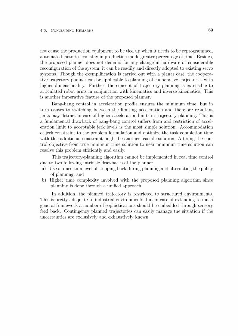
4.6. Concluding Remarks 69
not cause the production equipment to be tied up when it needs to be reprogrammed,automated factories can stay in production mode greater percentage of time. Besides,the proposed planner does not demand for any change in hardware or considerablereconfiguration of the system, it can be readily and directly adopted to existing servosystems. Though the exemplification is carried out with a planar case, the coopera-tive trajectory planner can be applicable to planning of cooperative trajectories withhigher dimensionality. Further, the concept of trajectory planning is extensible toarticulated robot arms in conjunction with kinematics and inverse kinematics. Thisis another imperative feature of the proposed planner.
Bang-bang control in acceleration profile ensures the minimum time, but inturn causes to switching between the limiting acceleration and therefore resultantjerks may detract in case of higher acceleration limits in trajectory planning. This isa fundamental drawback of bang-bang control suffers from and restriction of accel-eration limit to acceptable jerk levels is the most simple solution. Accommodationof jerk constraint to the problem formulation and optimize the task completion timewith this additional constraint might be another feasible solution. Altering the con-trol objective from true minimum time solution to near minimum time solution canresolve this problem efficiently and easily.
This trajectory-planning algorithm cannot be implemented in real time controldue to two following intrinsic drawbacks of the planner,a) Use of uncertain level of stepping back during planning and alternating the policy
of planning, andb) Higher time complexity involved with the proposed planning algorithm since
planning is done through a unified approach.
In addition, the planned trajectory is restricted to structured environments.This is pretty adequate to industrial environments, but in case of extending to muchgeneral framework a number of sophistications should be embedded through sensoryfeed back. Contingency planned trajectories can easily manage the situation if theuncertainties are exclusively and exhaustively known.

70 4. Minimum Time Cooperative Control of Two Robots
0 0.2 0.4 0.6-1
0
1
0 0.2 0.4 0.60.14
0.145
0.15
0.155
0 0.2 0.4 0.60.28
0.29
0.3
0.31
0 0.2 0.4 0.6-0.06
-0.03
0
0.030 0.2 0.4 0.60.14
0.145
0.15
0.155
0 0.2 0.4 0.6
-0.05
0
0.05
0 0.2 0.4 0.6-0.05
0
0.05
0 0.2 0.4 0.6-1
0
1
0 0.2 0.4 0.6-1
0
1
0 0.2 0.4 0.6-1
0
10 0.2 0.4 0.6-0.03
0
0.03
0.06
Time [s] Time[s] Time[s] Time[s]
Posi
tion
[m
]V
eloc
ity
[m/s
]A
ccel
erat
ion
[m/s
2 ]
0 0.2 0.4 0.60.29
0.3
0.31
0.32
Robot A - X Robot A - Y Robot B - X Robot B - Y
Figure 4.7: Minimum Time Input Cooperative Trajectory of Two Cartesian Robots forS-Shaped Locus
0 0.2 0.4 0.6 0.8-0.6-0.3
00.30.6
0 0.3 0.6 0.90.15
0.16
0.17
0.18
0 0.3 0.6 0.9
0.33
0.34
0.35
0 0.3 0.6 0.9-0.1
-0.050
0.050.1
0 0.3 0.6 0.90.15
0.16
0.17
0.18
0 0.3 0.6 0.90
0.02
0.04
0.06
0 0.3 0.6 0.90
0.02
0.04
0.06
0 0.3 0.6 0.9-0.6-0.3
00.30.6
0 0.3 0.6 0.9-0.6-0.3
00.30.6
0 0.3 0.6 0.9-0.6-0.3
00.30.6
0 0.3 0.6 0.9-0.1
-0.050
0.050.1
Time [s] Time[s] Time[s] Time[s]
Posi
tion
[m]
Vel
ocity
[m
/s]
Acc
eler
atio
n [m
/s2 ]
0 0.3 0.6 0.90.35
0.36
0.37
Robot A - X Robot A - Y Robot B - X Robot B - Y
Figure 4.8: Minimum Time Input Joint Space Trajectory of Two Cartesian Robot forV-Shaped Locus
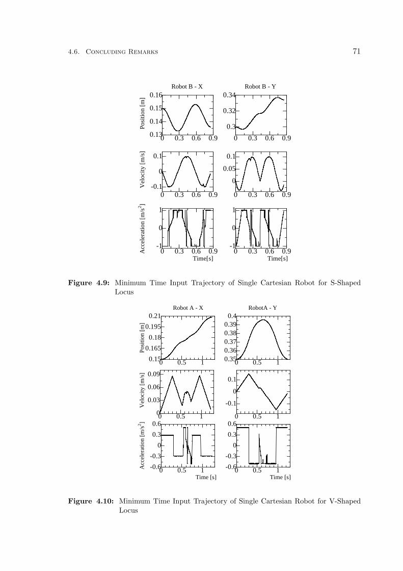
4.6. Concluding Remarks 71
0 0.3 0.6 0.9
0.3
0.32
0.34
0 0.3 0.6 0.9-0.1
0
0.1
0 0.3 0.6 0.9
0
0.05
0.1
Time[s]Time[s]
Robot B - X Robot B - Y
Posi
tion
[m]
Vel
ocity
[m
/s]
Acc
eler
atio
n [m
/s2 ]
0 0.3 0.6 0.90.13
0.14
0.15
0.16
0 0.3 0.6 0.9-1
0
1
0 0.3 0.6 0.9-1
0
1
Figure 4.9: Minimum Time Input Trajectory of Single Cartesian Robot for S-ShapedLocus
0 0.5 10.350.360.370.380.39
0.4
0 0.5 10
0.03
0.06
0.09
0 0.5 1
-0.1
0
0.1
0 0.5 1-0.6
-0.3
0
0.3
0.6
0 0.5 1-0.6
-0.3
0
0.3
0.6
Time [s] Time [s]
Pos
ition
[m
]
0 0.5 10.15
0.165
0.18
0.195
0.21
Vel
ocity
[m
/s]
Acc
eler
atio
n [m
/s2 ]
Robot A - X RobotA - Y
Figure 4.10: Minimum Time Input Trajectory of Single Cartesian Robot for V-ShapedLocus

72 4. Minimum Time Cooperative Control of Two Robots
0 0.2 0.4 0.60.4998
0.4999
0.5
0.5001
0.5002
0.5003
Time[s]
Cum
ulat
ive
cont
ribu
tion
of
robo
t A [
%]
Figure 4.11: Cumulative Contribution of Robot A in Cooperative Control of Two Carte-sian Robots for S-Shaped Locus
0 0.2 0.4 0.60
0.05
0.1
0.15
Time[s]
Tan
gent
ial c
oope
rati
ve
spe
ed [
m/s
]
Figure 4.12: Tangential Cooperative Velocity Profile for S-Shaped Locus

4.6. Concluding Remarks 73
0 0.3 0.6 0.90
0.05
0.1
0 0.3 0.6 0.90
0.1
0.2
Cooperative velocity
Cooperative speed along the locus
Time [s] Time [s]
Time [s]
X-d
irec
tion
[m
/s]
Y-d
irec
tion
[m
/s]
Tan
gent
ial [
m/s
]0 0.3 0.6 0.9-0.2
-0.1
0
0.1
0.2
Figure 4.13: Tangential and Cooperative Velocity Profiles for V-Shaped Locus
0 0.01 0.02 0.03 0.04 0.05 0.06-0.05
-0.04
-0.03
-0.02
-0.01
0Cooperative space locus
Y [
m]
X [m]
Figure 4.14: V-Shaped Locus in Work Space

Chapter 5
Conclusions andRecommendations
Two key important areas - belt drives and cooperative control to speed up, have beenused to demonstrate the trajectory planning scenarios for servo controlled objects.The overall goal of this thesis is to develop a feasible technique for vibration restraintaccurate position control of belt driven machines under high-speed operations and tosynthesize advanced trajectory planner for cooperative control of two robot arms. Theunderstanding and the applications of the proposed methods are realized substantiallyby this work. Although a brief summery of each chapter is provided at the end of therespective chapter, this chapter deals with comprehensive discussions of the overallwork in chapterwise. Possible future research directions that can be originated fromthis study are also included in this chapter.
5.1 Conclusions
The thesis covers the theoretical developments on1. Model construction of a belt driven machine,2. Management of computational complexity of the cooperative trajectory planning
through short-listing criterion,3. Derivation of minimal acceleration forth order spline scheme and,4. Philosophical notions and mathematical analysis on minimum time cooperative
trajectory planningto generate
1. Accurate high-speed position control of bet drives with vibration restraint,2. Complementary trajectories of two articulated robot arms for a specified ob-
jective cooperative trajectory under fair task distribution strategy subjected tojoint acceleration constraints and,
3. Minimum time complementary trajectories of two Cartesian robots for a givencurvy locus under maximum joint acceleration constraints.
The effectiveness of the proposed methods was verified with simulation stud-ies followed by solid confirmation through experiments. The proposed vibration re-straint techniques were implemented and experimentally tested with an actual beltdriven machine and the cooperative trajectory planner for articulated robots was in-strumented with two industrial robot manipulators Performer MK2 and MK3. Theperformance improvement by the proposed trajectory planners was demonstrated interms of task completion time, error profiles and tracking profiles. Implementation
74

5.2. Significant Remarks 75
friendliness feature of all above three approaches makes them conveniently incorpo-rated to the present industrial servo systems and it is one of the vital characteristicsof the proposed techniques.
In chapter 2, stepwise derivation of an accurate model integrating the beltreaction torque was discussed. Design of a feed forward dynamic compensator torestrain vibrations and to overcome delay dynamics has been reviewed.
Decomposition of objective cooperative trajectory between two articulated robotarms based on the complementary action, in view of increasing the speed of operationby exceeding the dynamic bounds of individual robot, was investigated in chapter 3.Specifications for the cooperative trajectory to be achieved such as maximum coop-erative speed and maximum cooperative acceleration, determined by the applicationitself are inputs to the system and fair task distribution becomes an integral part ofcontrol objective under limited acceleration of joints. Two stage trajectory planningparadigm has been devised to reduce the time and space complexity, intact with therequired level of accuracy. Segment level planning while optimizing the cost functionon regular task distribution, generates the trajectory through the knot points andthe short-listing criteria has been exploited as a means of resolving insurmountablecomputational overhead to a manageable level. Optimum forth order spline schemederived interpolates the knot points such that the acceleration of the entire trajectoryis kept at a minimum while guaranteeing the guidance through via points.
Chapter 4 contemplates on a time optimal cooperative control of two Cartesianrobots along a given curvy path under the maximum joint acceleration constraint.A bang-bang control scheme in acceleration has been proposed to realize minimumtime in cooperative control. Philosophical aspects behind the proposed algorithmwere disclosed and necessity of the stepping back to avoid no solution condition wasmathematically justified. Fairness in task distribution at each planning stage wasensured through the conformation of even task assignment constraint.
5.2 Significant Remarks
At the end of the thesis, the author would review his three-year Ph.D. work in Naka-mura laboratory, Department of Advanced Systems Control Engineering, GraduateSchool of Science and Engineering, Saga University, Japan.
When he first entered this laboratory, his supervisor Prof. Masatoshi Nakamuragave him several suggestions and recommendations. The deepest impression amongthem was that, his researches were not only standing on theoretical research, butalso were combining with applications, especially paying much attention on collabo-ration and cooperation with the industry. The author participated quarterly researchdiscussions on mechatronics with Yasakawa Company and particularly with Prof.Kyura, Department of Electrical Engineering, Kinki University (in Kyushu). It couldunderstand the currently existing problems in the industry. The fruitful discussionsimparted a valuable insight to practical perspectives and exposed the author to realindustrial issues on control and manufacturing. The knowledge gained through theseresearch discussions immensely helped to carefully identify the real research problems

76 5. Conclusions and Recommendations
and to develop the solution strategies proposed in this thesis.
A person whom the supervisor Masatoshi Nakamura suggests to memorize isthe founder of the Cybernetics-Norbert Wiener. His books [86]-[88] equipped theauthor with not only basic control knowledge, but also the Wiener’s considerationsof the way to develop research, especially the research in control field. Some excerptsin Wiener’s book [86] are noteworthy to indicate here, particularly the followingparagraph in introduction.
A century ago there may have been no Leibniz, but there was a Gauss, Faradayand a Darwin. Today there are few scholars who can call themselves mathematiciansor physicists or biologists without restriction. A man may be a topologist or an acous-tician or a coleopterist. He will be filled with a jargon of his field, and will know all itsliterature and its ramifications, but, more frequently than not, he will regard the nextsubject as something belonging to his colleague three doors down the corridor, and willconsider any interest in it on his own part as unwarrantable breach of privacy.
After Wiener made the above sentences in his book, more than thirty-five yearshas been past. We are now encountering more and more complex control problems. AsWiener pointed out, researchers should master various disciplines instead of restrictingin one field. We must know the current scientific development that is being undertakenby the researcher three doors down the corridor, otherwise,
If a physiologist who knows no mathematics works together with a mathemati-cian who knows no physiology, the one will be unable to state his problem that theother can manipulate, and the second will be unable to put the answers in any formthat the first can understand.
To achieve a successful cooperation for researchers from different fields, WienercommentedThe mathematician need not have the skill to conduct a physiological experiment, buthe must have the skill to understand one, to criticize one, and to suggest one. Thephysiologist need not to be able to prove a certain mathematical theorem, but he mustbe able to grasp its physiological significance and tell the mathematician for what heshould look.
The author feels very lucky to have a chance to get the know-how of researchand to learn how to start cracking research problems by bridging the existing gapsin the field of research as well as many other disciplines. Most importantly, he haslearnt the way to extend research work, which will be the fundamental backgroundfor his future study.
5.3 Recommendations for Further Developments
This section considers the state of art in robotics in light of cooperative requirementscum control objectives and thereby draws the potential futuristic directions. The fieldof robotics is still in its infancy, especially in cooperative behavior though the robotshave become economically feasible for a number of applications. Robots are stillslower than human in many tasks, but are already better than human in certain tasks

5.3. Recommendations for Further Developments 77
requiring high positional accuracy. Therefore, the research on robot speed is beingaddressed on several fronts. Limitations on computational speed are being addressedby steady improvements in microprocessor technology, by multiprocessor architecturesand by special purpose hardware for dynamic, kinematic and control computations.Despite these advances in computability control system performance is increasinglylimited by speed of computation. Coordinative behavior in cooperative trajectoryplanning in view of boosting up the speed is another consideration. However, theamount of research being done in strict cooperative control is disproportionately smallin comparison with its importance to increase the execution pace.
Narrowing down the general scope and focusing the attention directly onto thework covered by this thesis, I have achieved several objectives that are valuable forindustrial articulated robot arm applications in the industry and belt driven machinescontrol. However, the proposed new techniques open the room for many types ofsophistications and few of such directions can be stated in the recommendation forfurther developments in extending this thesis work.
5.3.1 Belt driven machine
1. Especially at low gear ratio of the belt driven machine, change in load inertia mayseriously affect the position control of belt drives under high-speed operation.In case of a belt driven robot, variation of inertia with the configuration ofrobot plays a major role in deteriorating the following trajectory. However,the belt driven machine used for experiment, works in a horizontal plane andhence such variation in inertia does not experience. Further, since the controllerCOSMOS takes the constant load inertia and motor inertia as control inputsspecified in a data file into account, in generating the control torque according tothe resident control algorithm, COSMOS cannot directly accommodate variableinertia of belt driven robots. Therefore, designing a new controller capableof accepting variable inertia, or devising some techniques to make the controllermuch more robust over variable inertia without sacrificing the vibration restraintand accurate positioning are open questions for the future.
2. The concept proposed for belt driven machine is tested with one degree of free-dom. A systematic extension can be made for multi-axis robot with decoupledjoint dynamics. However, dynamics cannot be assumed as decoupled in nature,principally at low gear ratios. Development of coupled dynamic model for multi-axis robot is a potential research theme yet to be addressed. However, powertransmission introduces a number of factors, including static friction, bindingwear, backlash, and cogging that make it difficult to model the motion pro-duced. The proposed feed forward dynamic compensator is still valid in such acoupled dynamical control scheme too.
3. Basic motive for the use of belt drives is to make the robot arm light weighted.Some low inertia meal assistant robots work on belt drives, but for such applica-tions, some sophistication should be made with an explicit force control schemeto guarantee that the force at the end effector does not exceed the predetermined
78 5. Conclusions and Recommendations
value since the safety of the human beings involved is paramount.
5.3.2 Cooperative trajectory planner for a given objective trajectory
1. The proposed trajectory-planning scheme is derived on the principles of kinemat-ics and hence direct control of force exerted does not under deliberate control.So the application is limited to non-force interactive control applications such aslaser cutting, contour welding and spraying. In order to extend the trajectoryplanner beyond this level, force control in addition to position control is manda-tory. Developments of new primitives for describing motion and the design ofcontrol systems capable of executing them directly through embodiment of forcecontrol scheme to the proposed algorithm has to be tried as a future direction.When adding up such key feature, a closed loop force control with sensory feedback is highly recommended, because it provides much flexibility and thus re-structures to a much general platform. Number of sophistications can be furtheradded through sensory feed back and thereby the trajectory-planning scheme canbe upgraded enabling to operate in unknown and ever changing environments.
2. The cooperative trajectory planning under strict coordination is achieved basedon the complementary principle. However, when extending it to cooperativecontrol of multiple robots, complementary principle is no more applicable andanother task distribution criterion along with optimization technique must beinstrumented. Therefore a complete revision of the algorithm is demanded whenextending it to multiple robots and the systematic adaptation of the proposedmethod is hard to be realized.
3. Since the proposed algorithm is established on the search principle for non-terminating solution while minimizing the difference in maximum joint veloci-ties of two robots, the generation of results is not deterministic in time. Besides,computation complexity involved with inverse kinematics and kinematics makesthe algorithm slow in execution time. Therefore, real time realization is notpossible in the present form and therefore it is used as an off-line planning tech-nique since off-line programming can absorb the real time intolerable time lags.Certain level of perfection in computational time can be achieved by contrivinga distributed computing architecture with parallel computation. However, con-struction of such system is a systematic project conceding substantial amountof resources. Therefore a development of a separate real time algorithm servingthe same planning objective seems to be more effective and still to be exploited.
4. Since the short-listing criterion restricts the search scope for solution as a meansof reducing the execution time of planning the cooperative trajectory, it doesnot always guarantee a global optimum solution, but a sub-optimal solution.Increasing the tolerance to cover a wider scope of the solution space and therebylooking for the highly probable global optimum is a self-defeating attempt asit exponentially increases the computational time. In the proposed approach,single robot solution is assumed to be the initial non-terminating solution toprobe for optimal solutions at its vicinity. Shifting the initial non-terminating

5.3. Recommendations for Further Developments 79
solution in some methodical way, in search of other sub-optimal solutions is apossible direction for global solution with the expense of computational time.Reformation of the existing algorithm or inventing a more effective analyticalalgorithm for global optimum solution is ahead for future work.
5.3.3 Minimum time cooperative trajectory planner of two Cartesian robotsunder given objective locus
1. The proposed minimum time cooperative trajectory planner is of bang-bangcontrol in acceleration profile, oscillating the acceleration between maximumlimits, at least of one joint of each robot is inevitable at certain points along thetrajectory. If the acceleration limit were adequately high, it would develop a sub-stantial jerk particularly at low sampling time. Consideration of jerk constraintfor minimum time trajectory planning is one option. Changing the cooperativeplanning objective to near time optimal might be another feasible solution toresolve higher jerk levels. Incorporation of jerk limits is an improvement to beadded to enhance the performance of corporative control.
2. Through parallel computing architectures backed with super power computa-tional hardware resources, computational time can be dramatically reduced.But the level of stepping back is unpredictable and it depends on case by case.Therefore, guaranteed real time performance could not be apprehended evenwith expedited architectures and better resources due to intrinsic drawback ofstepping back mechanism within the algorithm. Algorithmic revision for realtime is a timely research direction.
3. The proposed planner is basically developed for structured environment wherethe motion and the initial locations are a priori known. More accurate errorfree sensing systems embodied in the trajectory planning with time debuggingand error recovery capabilities are potential advancements that can be made tothe proposed planner, such that it can suitably appropriate for dynamic andinsufficiently known environments. Robot work cell configurability is anothersignificant issue in the design of new controller software and hardware to permitsensors and new motion primitives be easily integrated into the system. However,such crucial amendments require a considerable research effort and I believe thatit may be realizable in near future.
4. The following research themes and directives are emerged from the thesis workon minimum time cooperative control of two robots as prospective research di-rection.• Expand to multirobot trajectory planning under minimum time criterion• Subjugation of an issue of force interaction in cooperative control of two
robots, in view of speeding up the operation• Integration of smart and intelligence characteristics so that planning can
be done in unknown environments and dynamically changing environmentsduring task execution for autonomous cooperative purposes
• Exploitation of teleoperated cooperative control possibilities in minimumtime for rescue, undersea and space explorations.

Appendix A
Coordinate Systems andTransformations
A.1 Coordinate Systems for Spatial Description
Any point in space can be described by a coordinate system irrespective of its typeof definition i.e. Cartesian, spherical or any other. Selection of a fixed point in spacetermed as origin is a prerequisite to define a coordinate system. The way of measure-ment made from the origin determines the type of coordinate system and a minimumof three parameters is mandatory to uniquely indicate a point in space. However,the discussion is confined to Cartesian coordinate system, which is characterized bya mutually perpendicular right hand set composed of three axes originated from theorigin, along which the measurements are made. It is frequently used to represent apoint in space.
Though the translational location that is measured along the axis is adequateto describe a point in space completely, it is not sufficient to describe an objectsince an object has the freedom to rotate and eventually to give a new configuration.Therefore, an object in the space can be necessarily and sufficiently described withtwo aspects i.e. position and orientation. Considering the above two ascriptions of anobject together, it is termed as pose. Position is the translational location of a pointattached to an object or to an end effector and is usually expressed with respect toa base frame. Orientation is the rotational location of an object or of an end effectorwith respect to a reference coordinates system.
To describe the orientation of an object relative to the reference coordinatesystem that is already being defined for the representation of a point in space, anotherframe or a coordinate system, whose origin is a fixed point on the object, is attachedto the object and the description of this coordinate system is given relative to thereference system. Since any orientation could be achieved through a sequence ofrotations around three mutually perpendicular axes, a rotation vector with threetuples can uniquely express orientation. Representation of Euler angle illustrates thisscenario of rotation sequence, mathematically.
A.2 Mathematical Representation and Operations
Now, the depiction of pose of an object has been reduced to a mathematical prob-lem, which explains the relative arrangement of two coordinate systems. Translationand rotation are two fundamental applicable operations for two coordinate systems.
80

A.2. Mathematical Representation and Operations 81
Translation can completely express the relative positions of the origins of the twocoordinate systems whereas rotation describes the misalignments of the respectivecoordinate axes when two origins coincide with each other.
XA
YA
ZA
XB
YB
ZB P
Figure A.1: Translation and Rotation of Coordinate Systems
Referring to Fig.A.1, the position of point P is represented with respect to frame Aand frame B. The transformation of coordinate systems in pose can be mathematicallyexpressed in the form of matrix and given by
[AP1
]=
[ABP APBorg
0 0 0 1
] [BP1
](A.1)
where APBorg and ABP denote position of B’s origin with respect to frame A and
rotation matrix whose values are determined by
[ABR
]=
XBXA YBXA ZBXA
XBYA YBYA ZBYA
XBZA YBZA ZBZA
(A.2)
of which [Xk, Yk, Zk] denotes the direction vectors of frame k = A,B. The expressiongiven in A.1 is referred to as homogeneous transform and it is quite computationallyintensive as the multiplication is associated with a 4X4 matrix.
A robot can be considered as an open kinematic chain and hence this homoge-neous transformation could be directly applied to find the pose of the object undermanipulation. A three dimensional orthogonal coordinate system is basically definedsuch that the origin of the coordinate system lies on the base of the robot and it isdesignated as the base coordinate system. A coordinate frame for each link can beconveniently defined using DH notation and the pose of the object or the end effec-tor could be comprehensively determined by successive application of homogeneoustransform.

Appendix B
Space Transformation
B.1 Forward Kinematics and Inverse Kinematics
Kinematics is the science of motion that treats motion without regard to the forcesthat cause it. Therefore, in forward and inverse kinematics, forces are not considered.These are used to transform spatial description in position and orientation of the endeffector-pose from workspace to configuration (joint) space and vise versa.
Forward kinematics or direct kinematics calculates the end effector pose inCartesian coordinate description for a given set of joint positions. In more preciseterms, for a specified configuration vector, forward kinematics calculates the positionalone or the position and orientation of the tool frame with respect to the base frame.This relationship yields a unique solution.
Given the position and orientation of the end effector of the manipulator, inversekinematics calculates all the possible set of joint angles which could be used to attainthis given position and orientation. Inverse kinematic solutions can be grouped intoclosed form solutions and numerical solutions, which are computationally more ex-pensive and slower. Derivations of closed loop solutions are based on either algebraicmethods or geometric methods.
A manipulator is defined to be solvable, if all the sets of joint variables for agiven position and orientation can be determined by an algorithm either numericallyor analytically. Many manipulators have multiple solutions for a single configuration.Peiper [88] has shown that a general 6 degrees of freedom manipulator does not havea closed form solution. Besides, no solution conditions prevail at singularities inworkspace; inverse kinematics is not convenient as forward kinematics, especially athigher degrees of freedom. Even if inverse kinematic solutions are found, they maynot be physically realizable due to joint angle limitations.
Basically, these relationships are established considering either geometry (con-fined to limited cases), or transformation of coordinate systems attached to each link(much generic approach). Adoption of Denavit-Hartenberg convention for the assign-ment of coordinate frames on robot links is popular, since it immensely helps forconvenient transformation of coordinate frames.
The following figure depicts the definition of axis for PERFORMER MK3 robot.The rest of this section is devoted to establish the forward and inverse kinematicrelationship in 3D considering the position only.
82

B.1. Forward Kinematics and Inverse Kinematics 83
Y
k1θ
k3θ
k2θ
kl1
kl2
kl3
P(x,y,z)
Z
X
Figure B.1: Diagrammatic Representation of Robot’s Link Structure
Referring to the above figure forward kinematic relationship can be expressedby
xyz
=
lk1cos(θk1) + lk2cos(θ
k1)sin(θk
2) + lk3cos(θk1)sin(θk
2 + θk3)
lk1sin(θk1) + lk2sin(θk
1)sin(θk2) + lk3sin(θk
1)sin(θk2 + θk
3)lk2cos(θ
k2) + lk3cos(θ
k2 + θk
3)
(B.1)
where [x, y, z]T , [θk1 , θ
k2 , θ
k3 ]
T and lki denote the position vector in Cartesian space, theconfiguration vector in joint space and the length of link i of kth robot. The inversekinematics for the same is described by
θk1
θk2
θk3
=
tan−1(y/x)
tan−1(L/z)− cos−1
[L2+z2−(lk2 )2−(lk3 )2
2lk2√
L2+z2
]
cos−1
[L2+z2−(lk2 )2−(lk3 )2
2lk2 lk3
]
(B.2)
where L =√
x2 + y2 − lk1 . The length of the first link could be regarded as the offsetbetween first two links of the robot manipulator.
By differentiating B.1, mapping between the velocities in work and configurationspace can be determined as given by
xk1
yk2
zk3
= [J ]
θk1
θk2
θk3
(B.3)
where [J ] is referred to as Jacobian and its value is expressed by
[J ] =
−s1(l
k1 + lk2s2 + lk3s2,3) c1(l
k2c2 + lk3c2,3) lk3c1c2,3
c1(lk1 + lk2s2 + lk3s2,3) s1(l
k2c2 + lk3c2,3) lk3s1c2,3
0 −lk2s2 − lk3s2,3 −lk3s2,3
(B.4)
in that, si = sin(θki ), ci = cos(θk
i ), si,j = sin(θki + θk
j ) and ci,j = cos(θki + θk
j ).

Appendix C
An Overview of RobotManipulator System
C.1 Schematic Representation of Robot System
Schematics of a typical industrial robot manipulator (Performer MK3) are
D/A
A/D
Servo Controller
Robot manipulator
Reference input generator
Emergency switch
Figure C.1: Schematics of a Typical Robot Manipulator System
depicted in Fig.C.1. Basically, an industrial robotic system is composed of refer-ence input generator, data interface, servo controller, position and velocity sensors,mechanical structure of robot manipulator along with actuators, emergency switchand connecting wires. Reference input generator can be a standalone computer, orpreferably a computer connected to a network. Data interface converts digital datagenerated by reference input generator into its analog format so that it could beused by servo controller and to acquire analog sensor data of the robot manipulatorthrough servo controller. Each joint of the robot manipulator is equipped with anactuator, usually dc or ac servomotor, and sensors to measure position and velocity.Connecting wires establish the electrical connectivity while the emergency button isfor safety and it overrides all the operating functionalities.
C.2 Specifications of a Typical Industrial Robot
For a given vector of reference data [u1, u2, u3]T , P controller generates corresponding
velocity input, accounting the last configuration vector of the joints as specified byposition sensors and consequently fed it to servo controller for servo operation ofrobot actuators. The coding architecture explains the control of a single decoupledservo joint in detail and Table C.1 shows the set of control parameters for PerformerMK3 robot. For simplicity, second order model for servo system has been assumed to
84

C.3. Coding Architecture of a Revolute Joint 85
illustrate the coding architecture, but it is not necessarily be the second order model(please refer Appendix-D for details).
Table C.1: Control System Parameters
Parameter Denotation Value Shaft encoder resolution N 8192[pulse/rev] Gear ratio @joint 1 N1 120 Gear ratio @joint 2 N2 160 Gear ratio @joint 3 N3 160 Conversion factor of velocity pulse to voltage for joint 1
R1 0.000015161 [volt/(rad/s)]
Conversion factor of velocity pulse to voltage for joint 2
R2 0.000012484 [volt/(rad/s)]
Conversion factor of velocity pulse to voltage for joint 3
R3 0.000012169 [volt/(rad/s)]
C.3 Coding Architecture of a Revolute Joint
s
1
s
1
Sensor gain
SGE
vKRi CFi pK
Servo controller and robot structure Computer (controller)
+ + - -
[pulse]Pulseouti
outiθ
Modified input
taught data iniu
Figure C.2: Coding Architecture of a Single Decoupled Servo Joint
The modified input taught data uini [rad] is converted to Pulsein
i [pulse] by con-version factor CFi[pulse/rad] for the ith joint. The most of the control actions takeplace in pulse form to comply with the existing pulse counter. The reference pulse in-put Pulsein
i [pulse], is compared with the reading of the pulse counter Pulseouti [pulse]
so as to generate position error. The position loop gain of the ith joint transformsthis position error into velocity input V elocityin
i expressed in pulse per second. Thecoefficient Ri converts V elocityin
i into a quantity in voltage V oltini [volt], which lieswithin the acceptable bounds of input to the servo pack.
Velocity sensor connected to the ith joint reads the output velocity of the jointand sensor gain enhancer (SGE) conditions this signal to be compatible with voltage

86 C. An Overview of Robot Manipulator System
input V oltini [volt], so that the difference could be used to generate the velocity errorat joint i. Velocity loop gain transforms velocity error into acceleration and twosuccessive integrators convert acceleration into output position of joint i, θin
i .
The value of the conversion factor CFi corresponding to ith joint governs as
CFi =N ∗Ni
2π(C.1)
where N and Ni take the usual meaning as specified in Table C.1.

Appendix D
Famous Kinematic Models ofRobot Systems
Path planner gives the description of the path positions without timing andvelocity bounds, from which trajectory planner calculates its timing concerning thedynamics of the manipulator so as to give time history of positions and time deriva-tives. Manipulator characteristics could be represented either with a dynamic modelor with a kinematic model. In dynamic models, joint torques and forces are takeninto account while in kinematic models; no concern is paid to forces but resulting po-sitions, velocities and accelerations. Though the dynamic constraints are natural inexistence, they can be transformed into equivalent kinematic constraints (constant orpiecewise constant bounds), concerning the supremum (global minimum of maximum)of accelerations and velocities despite hampering 100% efficiency and capabilities ofmanipulators.
A detailed explanation of dynamic models is furnished in [43]. However, thisdiscussion is basically focused on popular and well-known kinematic models used forrobotic systems. Depending on the operational speed of the servo system and thedegree of influence of the simultaneous movements of other joints on a particularjoint, the selection of kinematic model may vary according to the accuracy required.On the assumption that the other joints have negligible effect, the joint dynamics canbe decoupled and as a result planning of trajectories will be easy.
D.1 First Order Kinematic Model
+
-
)(sU )(sθ
pKs
1
Servo Controller
Motor and mechanism
Position loop
Figure D.1: First Order Representation of Mechatronic Servo System
87

88 D. Famous Kinematic Models of Robot Systems
A decoupled joint of a mechatronic servo system can be mathematically repre-sented with a first order linear kinematic model as follows:
G(s) =Kp
s + Kp
(D.1)
where Kp is the position loop gain of the servo controller and it is briefly illustratedin Fig.D.1. The first order model can be used when the velocity of the servo motorsas the actuators of the mechatronic servo system is about 1/100 times of the ratedvelocity of motors [15].
D.2 Second Order Kinematic Model
Position loop
)(sθ
Velocity loop
Motor and mechanism
+
-
+
-
)(sU
vKpKs
1
s
1
Servo Controller
Figure D.2: Second Order Representation of Mechatronic Servo System
When the velocity of the motors are much faster, about 1/20 1/100 times ofthe rated velocity, the kinematics of the mechatronic servo system must be treatedas a second order model. The mechatronic servo system is described independentlyfor each axis with the second order model given below.
G(s) =KpKv
s2 + Kvs + KpKv
(D.2)
where Kv is the velocity loop gain as shown in Fig.D.2.
D.3 Fourth Order Kinematic Model
For higher velocities greater than 1/20 times of the rated speed, in other words high-speed operation of servo control joints, second order model can not represent thekinematics of joint adequately, as the reaction force/torque is considerably high andthe elastic deformation can not be further neglected. In such cases, fourth orderrepresentation of the decoupled servo joint can precisely illustrate the characteristicsand it is briefly shown in Fig.D.3.
Fourth order model of independent servo joint can mathematically expressed inthe following form:
G(s) =a0
a4s4 + a3s3 + a2s2 + a1s + a0
(D.3)

D.3. Fourth Order Kinematic Model 89
u
Servo Controller Motor and Mechanism
θ
Mθ PK gVK sJM
1LK
LD
s
1sJ L
1
Reaction force/torque
-
- -
+ ++ + +
- - s
1
Figure D.3: Fourth Order Representation of Mechatronic Servo System
where a0 = KpKLKgv , a1 = KLKg
v + KpDLKgv , a2 = KLJM + DLKg
v + KpJLKgv +
KLJL, a3 = DLJM + KgvJL and a4 = JLJM . In that case Kp, KL, Kg
v , JM and JL
denote position loop gain, elastic constant of the mechanism, servo amplifier gain,damping coefficient of the mechanism alone with load, motor inertia and load inertiarespectively. As the load inertia is a function of the manipulator configuration, thepayload and the shape of the payload, fourth order model is not a time invariantmodel.
When the joints move simultaneously, due to many functions including fric-tional, gravitational and inertial forces of the manipulator, one joint may be influ-enced by other joints. Therefore each joint can not be dissociated from the othersand therefore, model should be developed concerning the complete dynamics of themanipulator; not a single joint. Since, interactive joint model is highly dependanton the number of joints, the complexity proportionately increases as the number ofjoints is increased. Due to unavailability of generic model, interactive joint model isbeyond discussion here.

Appendix E
Generation of Minimum TimeTrajectory for a Single Robot
The S-shaped objective locus is basically composed of two circular arcs withequal radii, one appended below the other. Therefore geometrically, the objectivelocus is divided into two sections. Trajectory planning is carried out in forward andbackward directions along the two sections and finally they are merged into a singletrajectory. The following steps will concisely explain the algorithm employed to planthe minimum time trajectory of a single robot.
1. Parameterize the objective locusThe Cartesian coordinates of the objective locus can be related to a parameterλ as:x = pj + rs cos λy = qj + rs sin λ for j = 1, 2where (pj, qj) is the instantaneous center of the circular arc corresponding to thejth segment and rs is the radius of the circular arc.
2. Calculate the parameter values corresponding to initial and final positions of theeach section of the locus.
3. The following sequence of steps are reiterated for one section in the forwarddirection and in the reverse direction for the other.(a) Set a trial increment of parameter dλ during the sampling time Ts.(b) Calculate the new parameter value λnew = λold + dλ.(c) Calculate the new Cartesian position of the end effector (xnew, ynew).(d) Apply inverse kinematics and obtain the new joint positions [θnew
1 , θnew2 ] =
Inversekinematics(xnew, ynew).(e) Calculate the joint velocities and end effector velocity
θnewj = (θnew
j − θoldj )/Ts for j = 1, 2
vnew =√
(xnew − xold)2 + (ynew − yold)2/Ts.
(f) Calculate the joint accelerationsθnew
j = (θnewj − θold
j )/Ts for j = 1, 2.(g) Determine the indices corresponding to joint acceleration of two joints and
end effector velocity as:index1 = |θnew
1 |/θmax
index2 = |θnew2 |/θmax
index3 = |vnew|/vmax.Then assign the maximum of these three indices as the index account for dλ
90

91
modificationindex = max{index1, index2, index3}.
(h) If index /∈ [1 − δ, 1 + δ] then bisection method is applied to determine newvalue of dλ repeating steps b) through g), else move to step i). The term δgives the tolerance limit of index under consideration.
(i) Update the old parameter value with the new value (λold = λnew) and repeatsteps a) through h) in order to plan the subsequent trace of the trajectorycorresponding to ensuing sampling time, until new parameter value taken instep b) exceeds the limiting value of the section.
4. Concatenate the trajectories planned for each geometrical section of the locus.

Appendix F
Glossary of Terms
Accuracy The ability of a robot to reach a given point in space repeatedly andhow far off it will be in the worst case. Alternatively, the precisionwith which a computed point can be attained or measured.
Actuator A transducer that converts electrical, hydraulic, or pneumatic en-ergy to cause motion of the robot.
Analyticalmethods
Purely mathematical methods that do not require iteration.
Articulatedmanipulator
A manipulator with an arm that is broken into sections (links)by one or more joints. Each of the joints represents a degree offreedom in the manipulator system and allows translational androtary motion.
Axis A direction used to specify the robot motion in a linear or rotarymode.
Basecoordinates
The three dimensional orthogonal coordinate system which has theorigin on the robot base.
Cartesiancoordinates
A means for giving the location of a point in space by measuring itsdistance from a reference point along straight lines. The lines areat right angles to each other and all meet at the reference point.
Cartesianmanipulator
An arm with prismatic joints which allows movement along one ormore of the three- axes in the x, y, z coordinate system.
Closed-form A problem formulation that does not require iteration for its solu-tion.
Cognitive A machine that is aware of its surroundings. It is also able togenerate its own path plan and modify its task plan as necessary.
Compliance Displacement of a manipulator in response to a force or torque.
Continuouspath controlledrobot
A robot whose path is controlled by storing a large number or closesuccession of spatial points in memory during a teaching sequence.
Controlledpath
The path or mode of movement which ensures that the end of therobot’s arm will follow a predictable (controlled) path and orienta-tion as the robot travels from point to point.
92

93
Coriolis force The deflecting effect opposite to the direction of rotation when thevelocity of the robot arm is constant but the length of the armis changed. An opposing torque (in the direction of the rotation)must be applied to overcome this force. This can be done by havingthe robot arm retract while making a swing from one target pointto another.
Cybernetics The science or study of communication and control mechanisms inhuman and machine systems, including computers.
Degree offreedom
Regardless of the anatomy and type of movement, either rotationalor a translational, the number of independent ways in which theend effecter can move. It is defined by the number of rotational ortranslational axes through which motion can be achieved.
Dynamicmodel
A mathematical model describing the motions of the robot and theforces that cause them.
Dynamics The study of motion with regard to forces which cause the motion.
End effector An accessory device or tool specifically designed for attachment tothe robot wrist or tool mounting plate of the last link to enable therobot to perform its intended task.
Forwardkinematics
For a given set of joint angles, forward kinematic computes the po-sition and orientation of tool frame relative to the base frame. Inother words it transforms joint space (configuration space) descrip-tion into Cartesian space (task space, operational space or workspace) description.
Gantry robot A robot which has three degrees of freedom along the X, Y, andZ coordinate system. Usually consists of a spooling system (usedas a crane) which when reeled or unreeled provides the up anddown motion along the Z axis. The spool can slide from left toright along a shaft which provides movement along the Z axis. Thespool and shaft can move forward and back along tracks, whichprovide movement along the Y axis. Usually used to position it’send-effector over a desired object and pick it up.
Hardautomation
Automated machinery that is fixed, or dedicated, to one particu-lar manufacturing task throughout its life. Fixed automation is asynonym for hard automation.
Hybridcontrol
A control scheme in which some directions are controlled by positioncontrol law and the remaining directions are controlled by forcecontrol law.
Incrementalmovement
Movement is broken up into very small pieces, and then takes oneat a time.
Industrialrobot
A reprogrammable, multifunctional manipulator designed to movematerial, parts, tools, or other devices through variable pro-grammed motions for the performance of a variety of tasks. Theprinciple components are: one or more arms that can move in sev-eral directions;

94 F. Glossary of Terms
Inversekinematics
Given the position and orientation of the end effector of the ma-nipulator, inverse kinematics calculate all the possible set of jointangles which can be used to attain this given position and orienta-tion.
Iteration Repeatedly applying a series of predefined operations to progres-sively advance towards a solution.
Jacobian Specify a mapping from velocities in joint space to velocities inCartesian space.
Joint A part of the manipulator system which allows a rotation or trans-lational degree of freedom to a link or end-effector.
Joint space A coordinate system used to describe the state of the robot in termsof its joint states. This is also referred to as configuration space.
Kinematics Science of motion that treats motion without regard to the forceswhich cause the motion. Kinematics of manipulators refers to allthe geometric and time based properties of the motion.
Lagrangemultipliers
A mathematical technique for transforming equality constraintsinto performance criteria, thus expressing a constrained problemas an unconstrained problem.
Lead throughprogramming
A means of teaching a robot by leading it through the operatingsequence with a control console or a hand-held control box.
Link A rigid part of a manipulator which connects adjacent joints.
Locus The special description of the end effector without consideration ofits timing. The term path has the same meaning.
Manipulator A robotic mechanism consisting of an arm and an end-effector. Itcontains a series of segments, jointed or sliding relative to one an-other, for the purpose and moving objects. The manipulator usuallyhas several degrees of freedom. It includes the arm, the wrist, andthe end-effector.
Off-lineprogramming
A means of programming a robot by developing a set of instructionson an independent computer and then using the software to controlthe robot at a later date.
Open-loopcontrol
A robotic control system in which data flows only from the con-troller to the mechanism and does not flow from the mechanismback to the controller. This does not allow self-correcting actionwhich can be provided with feedback.
Opticalencoder
A detection sensor which measures linear or rotary motion by de-tecting the movement of markings past a fixed beam of light. Thiscan be used to count revolutions, identify parts, etc.
Orientation The rotational location of an object or an end effector with respectto the reference coordinate system.
Parameter A set of constant factors applied to a particular situation.

95
Path points Include all the via points plus the initial and final points.
Payload The maximum amount of weight that a robot can handle withoutcausing harm, or malfunction to the robot under normal operationalconditions.
Pendantteaching
The mapping and recording of the position and orientation of arobot and/or manipulator system as the robot is manually movedin increments from an initial state along a path to a final goalstate. The position and orientation of each critical point (joints,robot base, is recorded and stored in a database for each way pointthe robot passes through on its trek toward its final goal. The robotmay now repeat the trek on its own by following the path stored inthe database.
Point-to-point motion
A type of robot motion in which a limited number of points alonga path of motion is specified by the controller, and the robot movesfrom one discrete point to another rather than in a continuous,smooth path.
Pose Position and orientation taken together.
position The translational location of a point attached to an object or to anend effector specified with respect to the base frame.
Positioncontrol
A technique which suppresses disturbances that perturb the sys-tem from the desired trajectory by calculating the velocity; andpositioning necessary to counteract such disturbances.
Precision (es-timatedparameter)
The precision of an estimate of a parameter in a model is a measureof how variable the estimate would be over other similar data sets.A very precise estimate would be one that did not vary much overdifferent data sets. Precision does not measure accuracy. Accuracyis a measure of the closeness of the estimate is to the real value ofthe parameter. Accuracy is measured by the average distance overdifferent data sets of the estimate from the real value.
Prismaticjoint
A joint of two nested links that slide onto or alongside of each other.
real timesystem
A real-time system is a system in which the correctness of the sys-tem behavior depends not only on the logical results of the compu-tations, but also on the physical instants at which these results areproduced. A Real-Time System responds in a (timely) predictableway to unpredictable external stimuli arrivals.
Redundancy Additional independent variables available than the constraints.
Repeatability The ability of the manipulator arm to position the end effecter at aparticular location within a specified distance from its position dur-ing the previous cycle. In other words, repeatability specifies howaccurately the manipulator can return to a given exact location.
Revolutejoint
The joints of a robot which are capable of rotary motion.

96 F. Glossary of Terms
Robot A robot is a re-programmable multifunctional manipulator designedto move material, parts, tools, or specialized devices through vari-able programmed motions for the performance of a variety of tasks.In practical usage, a robot is a mechanical device which performsautomated tasks, either according to direct human supervision, apre-defined program or, a set of general guidelines, using artificialintelligence techniques. These tasks either replace or enhance hu-man work, such as in manufacturing, construction or manipulationof heavy or hazardous materials. An automatic device that performfunctions normally ascribed to human or a machine in the form ofa human (Webster’s Dictionary).
Robotics Science of robots.
Servo-system A system in which the controller issues commands, motor drivesarms, and sensors measure the motions and signal the amount ofmotions back to the controller. This process is continued until thearm is repositioned to the point requested.
Singularity A position in the robot’s workspace where one or more joints nolonger represent independent controlling variables. Commonly usedto indicate a position where a particular mathematical formulationfails.
Spatialresolution
The minimum or smallest dimension to which the robot systemcan define the work space. This resolution determines the smallesterror that can be sensed by the robot, as limited by the minimumresolution of the controller or the minimum resolving increment ofthe servo-system.
Spline A smooth, continuous function used to approximate a set of func-tions that are uniquely defined on a set of sub-intervals. The ap-proximating function and the set of functions being approximatedintersect at a sufficient number of points to insure a high degree ofaccuracy in the approximation. This allows a robot manipulator tocomplete a task without jerky motion.
Statics The study of forces that do not cause motion.
Trajectory Refer to a time history of position, velocity and acceleration foreach degree of freedom.
Trajectorygeneration
The computation of smoothly controllable trajectory in multidi-mensional space which describes the desired motion of a manipula-tor.
Via point Intermediate locations or points in space in between the initial andfinal points through which a manipulator must pass en route to aparticular destination.
Work space The maximum reach space refers to all of the points or volume inspace that a robot’s end effector can possibly reach. The dexterousworkspace is all of the possible points or volume in space that arobot’s end effector can reach with an arbitrary orientation.
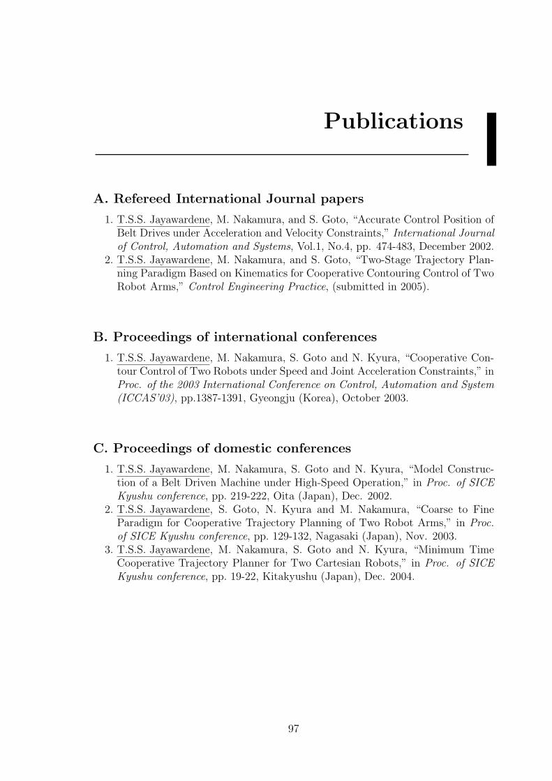
Publications
A. Refereed International Journal papers
1. T.S.S. Jayawardene, M. Nakamura, and S. Goto, “Accurate Control Position ofBelt Drives under Acceleration and Velocity Constraints,” International Journalof Control, Automation and Systems, Vol.1, No.4, pp. 474-483, December 2002.
2. T.S.S. Jayawardene, M. Nakamura, and S. Goto, “Two-Stage Trajectory Plan-ning Paradigm Based on Kinematics for Cooperative Contouring Control of TwoRobot Arms,” Control Engineering Practice, (submitted in 2005).
B. Proceedings of international conferences
1. T.S.S. Jayawardene, M. Nakamura, S. Goto and N. Kyura, “Cooperative Con-tour Control of Two Robots under Speed and Joint Acceleration Constraints,” inProc. of the 2003 International Conference on Control, Automation and System(ICCAS’03), pp.1387-1391, Gyeongju (Korea), October 2003.
C. Proceedings of domestic conferences
1. T.S.S. Jayawardene, M. Nakamura, S. Goto and N. Kyura, “Model Construc-tion of a Belt Driven Machine under High-Speed Operation,” in Proc. of SICEKyushu conference, pp. 219-222, Oita (Japan), Dec. 2002.
2. T.S.S. Jayawardene, S. Goto, N. Kyura and M. Nakamura, “Coarse to FineParadigm for Cooperative Trajectory Planning of Two Robot Arms,” in Proc.of SICE Kyushu conference, pp. 129-132, Nagasaki (Japan), Nov. 2003.
3. T.S.S. Jayawardene, M. Nakamura, S. Goto and N. Kyura, “Minimum TimeCooperative Trajectory Planner for Two Cartesian Robots,” in Proc. of SICEKyushu conference, pp. 19-22, Kitakyushu (Japan), Dec. 2004.
97

References
[1] http://cache.ucr.edu/∼currie/roboadam.htm
[2] Programmed Article Transfer, US Patent No. 2988237, 1961.
[3] H.A. Ernest, “A-Computer Controlled Mechanical Hand,” Sc.D thesis, Mas-sachusette Institute of Technology, Cambridge, 1961.
[4] E. Brussel, Websters Dictionary, Prentice Hall, 1988.
[5] http://www.frc.ri.cmu.edu/robotics-faq/1.html
[6] J.J. Craig, Introduction to robotics: Mechanics and Control, Addison Wesley,1989.
[7] http://www.cse.dmu.ac.uk/∼aayesh/teaching/robotics/CSCI2012/lec2012-01-1-2003.ppt
[8] D.E. Whitney, “State of the art and research needs in robot contact sensing,”in workshop on intelligent robots: Achievement and issues, SRI InternationalMenlo Park, pp. 137-144, 1984.
[9] L. Sciavicco and B. Siciliano, Modeling and Control of Robot Manipulators,Springer, 1995.
[10] M.W. Spong, F.L. Lewis and C.T. Abdallah, Robot control:Dynamic MotionPlanning and Analysis, IEEE Press, Newyork, 1992.
[11] K.S. Fu, R.C. Gonzalez and C.S.G. Lee, Robotics: Control, Sensing, Vision,and Intelligence, McGraw-Hill Book Company, 1987.
[12] B.G. Robert and S.A. Bortoff, “A Novel Approach to Vibration Reduction inFlexible Belt Drives,” in Topics in Control Theory and its Application, pp. 67-80, 1999.
[13] W. Li and X. Cheng, “Adaptive High Precision Control of Positioning Tables-Theory and Experiment,” in IEEE Transactions on Control Systems Technology,vol. 2, pp. 265-270, 1994.
[14] M. Nakamura, T. Iwanaga, S. Goto and N. Kyura, “High Speed High AccuracyPosition Control of Belt Drive Machine with Vibration Restraint,” in Proc. ofSICE Kyushu conference, pp. 359-362, Kumamoto (Japan), December 2001.
[15] S. Goto, M. Nakamura, and N. Kyura, “Modified Taught Data Method forIndustrial Mechatronic Servo Systems to Achieve Accurate Contour ControlPerformance,” in Proceedings of Advanced Intelligent mechatronics, AIM 97,1997.
[16] S.R. Munasinghe, M. Nakamura, S. Goto, and N. Kyura, “Pole Selection ofFeed Forward Compensators Considering Bounded Control Input of IndustrialMechatronic Systems,” in IEEE Transaction on Industrial Electronics, vol. 50,pp. 1191-1206, 2003.
98

References 99
[17] S.R. Munasinghe, M. Nakamura, S. Goto, and N. Kyura, “Pole Selection forModified Data Method for Mechatronic Servo Systems by Considering BoundedControl Input,” in Proc. of SICE Kyushu conference, pp. 183-186, Kumamoto(Japan), December 2001.
[18] K.M. Lee and C. Rutherford, “Frequency Reshaped Quadratic Control of a BeltDriven Robot,” in Proc. of Advanced Intelligent mechatronics, AIM 97, 1997.
[19] K.M. Lee and C. Rutherford, “Frequency Reshaped Quadratic Control of aLow-Cost Human Level Performance Belt Driven Robot,” in IEEE transactionon Mechatronics, vol. 9, pp. 95-110, 1999.
[20] K.G. Shin and N.D. Mckay, “Robust Trajectory Planning for Robotics Ma-nipulators under Payload Uncertainties,” in IEEE Transactions on AutomaticControl, vol. 32, pp. 1044-1054, 1987.
[21] K.G. Shin and N.D. Mckay, “Minimum Time Control of Robotic Manipulatorswith Geometric Path Constraints,” in IEEE Transactions on Automatic Control,vol. 30, pp. 531-541, 1985.
[22] L.V. Kavraki, P. Svestka, J.C. Latombe, and M.H. Overmars, “Probabilisticroad maps for path planning in high dimensional configuration space,” in IEEEtransactions on robotics and Automation, vol. 12, pp. 566-580, 1996.
[23] S. Lee and H. Moradi, “A real Time Dual Arm Collision Avoidance Algorithmfor Assembly,” in Journal of Robotics System, vol. 18, pp. 477-486, 2001.
[24] L.V. Kavraki, and J.C. Latombe, “Randomized processing of configurationspace for fast path planning,” in Proceedings of IEEE international conferenceon robotics and Automation, pp. 2131-2138, 1996.
[25] F. Fahimi and C. Nataraj, “Obstacle avoidance for spatial hyper redundantmanipulators using harmonic potential functions and mode shape technique,”in Journal of Robotics system, vol. 20, pp. 23-33, 2003.
[26] T.S.S Jayawardene, “Simulation Support Tool for Routing of AutomatedGuided Vehicles,” M.Sc. Thesis, University of Moratuwa, Sri Lanka, 2002.
[27] J.Y.S. Luh, M.W. Walker and R.P.C. Paul, “Resolved Acceleration Control ofMechanical Manipulators,” in IEEE Transactions on Automatic Control, vol. 25,pp. 468-474, 1980.
[28] R. Paul, “Manipulator Cartesian path control,” in IEEE transaction on systemman and cybernetics, vol. 9, pp. 702-711, 1979.
[29] S.R. Munasinghe, M. Nakamura, S. Aoki, S. Goto, and N. Kyura, “High SpeedPrecise Control of Robot Arm with Assigned Speed under Torque Constraint byTrajectory Generation in Joint Coordinates,” in Proc. of SMC 99, pp. 854-859,1999.
[30] R. Paul, Robert Manipulators, MIT Press Cambridge, 1981.
[31] G. Antonelli, S. Chiaverini, and Giuseppe, “Real-Time End-Effector Path Fol-lowing for Robot Manipulators Subject to Velocity, Acceleration, and Jerk JointLimits,” in Proc. of IEEE/ASME International Conference on Advanced Intel-ligent Mechatronic, Italy, pp. 452-457, 2001.

100 References
[32] D.F. Rogers, An introduction to NURBS with historical perspectives, MorganKaufmann, 2000.
[33] L.J.D. Plessis and J.A. Snyman, “Trajectory Planning through Interpolationby Overlapping Cubic Arcs and Cubic Splines,” in International Journal ofNumerical Methods and Engineering, vol. 57, pp. 1615-1641, 2003.
[34] K.G. Shin and N.D. Mckay, “A Dynamic Programming Approach to Trajec-tory Planning of Robotics Manipulators,” in IEEE Transactions on AutomaticControl, vol. 31, pp. 491-500, 1986.
[35] A.J. Cahill, M.R. James, J.C. Kiefer, and D. Williamson, “Remarks on theApplication of Dynamic Programming to Optimal Path Timing of Robot Ma-nipulators, ” in International Journal of Robust and Nonlinear Control, vol. 8,pp. 463-482, 1998.
[36] J.E. Bobrow, S. Dubowsky, and J.S. Gibson, “Time-Optimal Control of Roboticmanipulators along Specified Paths,” in The international journal of roboticsresearch, vol. 4, pp. 3-17, 1985.
[37] K.G. Shin and N.D. McKay, “An efficient robot arm control under geometricpath constraints,” in Proc. of IEEE conference on Decision and Control, SanFrancisco, 1983.
[38] K.G. Shin and N.D. Mckay, “Selection of Near Minimum Time Geometric Pathsfor Robot Manipulators,” in IEEE Transactions on Automatic Control, vol. 31,pp. 501-511, 1986.
[39] J.J.E. Slotine and H.S. Yang, “Improving the efficiency of time optimal pathfollowing algorithms,” in IEEE transaction on Robotics Automation, vol. 5,pp. 118-124, 1989.
[40] S.S. Han, S.B. Chol, J.H. Kim, “Position control of a flexible Granty robotarm using smart material actuators,” in Journal of Robotics System, vol. 16,pp. 581-595, 1999.
[41] P.S. Ghandi and F.H. Ghorbel, “Closed Loop compensation of Kinematic Errorin Harmonic Drives for Precision Control Applications,” in IEEE Transactionson Control Systems Technology, vol. 10, pp. 759-768, 2002.
[42] B.C.O. Maciel, M.H. Tera, and M. Bergerman, “Optimal Robust Controlof Under-actuated Manipulators Via Actuation Redundancy,” in Journal ofRobotics System, vol. 20, pp. 635-648, 2003.
[43] H.G. Sage, M.F. de Mathelin and E. Ostertag, “Robust Control of Robot Manip-ulators: a Survey,” in International Journal of Control, vol. 72, pp. 1498-1522,1999.
[44] N. Xi, T.J. Tarn and A.K. Bejczy, “Intelligent planning and control for multirobot coordination: An event based approach,” in IEEE Transactions onRobotics and Automation, vol. 12, pp. 439-452, 1996.
[45] J.S. Gu and C.W. de Silva, “Development and implementation of a real

References 101
time open architecture control system for industrial robot systems,” in En-gineering applications in Artificial Intelligence, article in press available onwww.sciencedirect.com.
[46] F. Caccavale, S. Chiaverini, C. Natale, B. Siciliano, L. Villani, “Geometricallyconsistent impedance control for dual-robot manipulation,” in Proc. of 2000IEEE International Conference on Robotics and Automation, San Francisco,pp. 3873-3878, 2000.
[47] F. Caccavale, C. Natale, B. Siciliano, L. Villani, Interaction control, pp. 121-154, Lecture Notes in Control and Information Sciences 270, Springer-Verlag,Heidelberg, 2001.
[48] B. Siciliano and L. Villani, “Six-degree-of-freedom impedance robot control,”,in Proc. of 8th International Conference on Advanced Robotics, pp. 387-392,Monterey, 1997.
[49] F. Caccavale, C. Natale, B. Siciliano, and L. Villani, “Resolved AccelerationControl of Robot Manipulators: A Critical Review with Experiments,” in Robot-ica, vol. 16, pp. 565-573, 1998.
[50] N.J. Koivo and T.H. Guo, “Adaptive Linear Controller for Robotics Manipula-tors,” in IEEE Transactions on Automatic Control, vol. 21, pp. 162-171, 1983.
[51] M.W. Spong, F.L. Lewis, and C.T. Abdallah, Robot Control: Dynamics, MotionPlanning and Analysis, IEEE press,1993.
[52] A.K. Swain and A.S. Morris, “A Unified Dynamic Model Formulation forRobotics Manipulator Systems,” in Journal of Robotics System, vol. 20, pp. 601-620, 2003.
[53] L. Sciavicco, B. Siciliano, and L. Villani, “Lagrange and Newton-Euler DynamicModeling of Gear Driven Rigid Robot Manipulator with Inclusion of MotorInertia Effect,” in Advanced Robotics, vol. 10, pp. 317-334, 1996.
[54] M. Brady, J.M. Hollerbach, T.L. Johnson, T. Lozano-Perez, M.T. Mason, RobotMotion: Planning and control, MIT press, 1998.
[55] T. Zhang, “High precision contour control of industrial articulated robot armby Gaussian neural network,” PhD dissertation submitted to Saga UniversityJapan, September 2002.
[56] J.Y.S. Luh, M.W. Walker, R.P.C. Paul, “On-line computational scheme formechanical manipulators,” in Journal. of Dynamics. System. Measurement. AndControl, vol. 102, pp. 69-76, 1980.
[57] J.J. Zhang, Y.F. Lu, B.Wang, “A non-recursive Newton-Euler formulation forthe parallel computation of manipulator inverse dynamics,” in IEEE transac-tions on. Systems Man and Cybernetics, vol. 28, no. 3, pp. 467-471, Aug., 1998.
[58] S. Dobowsky and T.G. DesForges, “The application of model reference adap-tive control to robotics manipulators,” in SME journal of dynamic systems,measurement and control, pp. 193-200, 1979.

102 References
[59] C.S.G. Lee and M.J. Chung, “An adaptive control strategy for mechanical ma-nipulators,” in IEEE transaction on automatic control, vol. 29, pp. 837-840,1984.
[60] J.Y.S. Luh and Y.F. Zheng, “Constrained relations between two coordinated in-dustrial robots for motion control,” in International Journal of robotics research,vol. 6, pp. 60-70, 1987.
[61] S. Hayati, “Hybrid position and force control of multi-arm cooperating robots,”in Proc. of IEEE conference on Robotics and automation, San Francisco, pp. 82-89, 1986.
[62] F. Caccavale and L. Villani, “An Impedance Control Strategy for CooperativeManipulation,” in Proc. of International Conference on Advanced IntelligentMechatronics, pp. 343-348, 2001.
[63] S. Abrate, “Vibrations of Belts and Belt Drives,” in Mechanism and MachineTheory, vol. 27, pp. 645-659, 1992.
[64] O. Khatib, K. Yokoi, K. Chang, D. Ruspini, R. Holmberg, A. Casal andA. Baader, “Force Strategies for Cooperative Tasks in Multiple Mobile Manipu-lation Systems,” in International Symposium of Robotics and Research, Munich,1995.
[65] K.S. Chang, R. Holmberg, and O. Khatib, “The Augmented Object Model:Cooperative Manipulation and Parallel Mechanism Dynamics,” in Proc. of IEEEinternational conference on Robotics and Automation, San Francisco, pp. 475-477, 2000.
[66] C.R. Carignan, D.L. Akin, “Cooperative Control of Two Robot Arms in theTransport of Inertial Load under Zero Gravity,” in IEEE Transactions onRobotics and Automation, vol. 4, pp. 414-419, 1988.
[67] K. Nagai, S. Iwasa, K. Watanabe, and H. Hanafusa, “Cooperative Control ofDual Arm Robots for Reasonable Motion Distribution,” in Proc. of InternationalConference on Intelligent Robots and Systems, Pittsburgh, Pennsylvania, Aug.1995.
[68] M. Bonert, L.H. Shu, and B. Benhabib, “Motion Planning for Multi-robot As-sembly System,” in Proc. of ASME: Design Engineering Technical Conference,Blacksburg, Jun. 1999.
[69] F. Caccavale, C. Natale, B. Siciliano and L. Villani, “Achieving a CooperativeBehavior in a dual Arm Robot System via a Modular Control Structure,” inJournal of Robotics System, vol. 18, pp. 691-700, 2001.
[70] M. Nakamura, S. Goto and N. Kyura, Mechatronic servo system control,Springer-Verlang, Berlin, Heidelberg, 2004.
[71] Baldor electric company, Motion Control Application notes, Baldor motors anddrives, pp. 23-25, 2002.
[72] R. Murphy, and P.M. Pardalos, Cooperative Control and Optimization, KluwerAcademic Publishers, 2002.

References 103
[73] Y.U. Cao, A. Fukuage, and A. Kahng, “Cooperative mobile robotics: An-tecedent and directions,” in Autonomous robots, vol. 4, pp. 7-27, 1997.
[74] R. Murphy, “conference on cooperative control and optimization open discus-sion,” in conference on cooperative control and optimization, Florida, 2001.
[75] L.E. Parker, “Adaptive heterogeneous multi-robot teams,” in Neural networksand their applications, vol. 28, pp. 75-92, 1999.
[76] J. Szewczyk, F. Plumet and P. Bidaud, “Planning and Controlling Robotsthrough Distributed Impedance,” in Journal of Robotics System, vol. 19,pp. 283-297, 2002.
[77] J.P. Desai and V. Kumar, “Motion Planning for Cooperating Mobile Manipu-lators, in Journal of Robotics System, vol. 16, pp. 557-579, 1999.
[78] J.F. Liu, K.A. Malek, “Robust Control of Planar Dual Arm Cooperative Manip-ulator,” in Robotics and Commuter Integrated Manufacturing, vol. 16, pp. 109-120, 2000.
[79] L.T. Wang and M.J. Kuo, “Time Optimal Constant Speed Motion Programmefor Multiple Cooperating Manipulators,” in Journal of Robotics System, vol. 16,pp. 185-194, 1999.
[80] L.E. Parker, “Alliance:An Achitecture for Fault Tolerant Multirobot Coopera-tion,” in IEEE Transactions on Robotics and Atomation, vol. 14, pp. 220-240,1998.
[81] E. Tunstel, M.A.A. de Oliveira, and S. Berman, “Fuzzy Behavior Hierarchies forMulti-Robot Control,” in International Journal of Intelligent Systems, vol. 17,pp. 449-470, 2002.
[82] J.T. Wen and K.K. Delgado, “Motion and Force Control of Multiple RoboticManipulators,” in Automatica, vol. 28, pp. 729-743, 1992.
[83] D. Sun and Y. Liu, “Position and Force Tracking of a Two-Manipulator SystemManipulating a Flexible Beam,” in Journal of Robotic Systems, vol. 18, pp. 197-212, 2001.
[84] M.A. Ridao, E.F. Camacho, J. Riquelme and M. Toro, “An Evolutionary andLocal Search Algorithm for Motion Planning of Two Manipulators,” in Journalof Robotics System, vol. 18, pp. 463-476, 2001.
[85] Y.P. Chien, Q. Xue, and Y. Chen, “Configuration Space Model of Tightly Coor-dinated Two Robot Manipulators Operating in 3D Workspace,” in IEEE Trans-actions on Systems, Man and Cybernetics, vol. 25, pp. 695-704, 1995.
[86] N. Wiener, Cybernetics or control and communication in the animal and ma-chine, The MIT press, MIT, 1965.
[87] N. Wiener, Extrapolation, interpolation, and smoothing of stationary time series,The MIT press, MIT, 1970.
[88] D. Pieper and B. Roth, “The Kinematics of Manipulators under ComputerControl,” in Proc. of the Second International Congress on Theory of Machinesand Mechanisms, vol. 2, pp. 159-169, Zakopane (Poland), 1969.