Embed Size (px)
Citation preview

Trajectory design for the Solar Orbiter mission
G. Janin
European Space Operations Centre.
European Space Agency.
64293 Darmstadt, Germany.
Monografıas de la Real Academia de Ciencias de Zaragoza. 25: 177–218, (2004).
Abstract
The Solar Orbiter project was approved on 12 September 2000 as ESA flexi-
mission F2 (Ref. [11]). This mission aims to: (i) explore the uncharted innermost
regions of our solar system, (ii) study the Sun from close-up (45-50 solar radii, or
0.21 AU), (iii) fly-by the Sun, tuned to its rotation and examine the solar surface and
the space above from a co-rotating vantage point, (iv) provide images of Sun’s polar
regions from heliographic latitudes as high as 38◦. Following a cruise phase including
five Solar Electric Propulsion arcs and three planetary Gravity Assist Manoeuvres
(GAM, Venus-Earth-Venus), an heliocentric orbit with a perihelion between 45 and
50 solar radii and a period of about 150 days will be reached after 1.9 year. Launch
in 2012 is foreseen from Baikonur with a Soyuz/ST launcher equipped with a Fre-
gat upper stage. After 1.2 year of prime science mission, a mission extension is
proposed. By adjusting the heliocentric orbit period such that it is commensurable
with the period of the orbit of Venus (a 3:2 resonant orbit is selected), an increase
of the inclination will be achieved by a series of successive Venus GAMs. It involves
no mid-course manoeuvres other than navigation manoeuvres. Performing 4 Venus
GAMs along 3.7 years, the inclination relative to the solar equator can be raised up
to 38◦.
Key words and expressions: Design of trajectories, Solar Orbiter project, gravity
assist manoeuvres.
MSC: 70F10, 76B75.
1 Introduction
The Solar Orbiter mission was first investigated at ESA in 1999 in the frame of the
Concurrent Design Facility (CDF) located at ESTEC. Kick-off meeting occurred on 1999
177
March 25 and the first technical definition study session was hold on April 29. At this
time, a preliminary Mission Analysis input was presented. Based mostly on Russian
investigations, ways to reach the desired low aphelion orbit and high inclination orbit
were proposed using GAMs or Solar SEP. It turned out that both ways lead to long
transfer duration or high ∆V requirements.
A similar problem was encountered with ESA mission BepiColombo toward Mercury.
For the transfer to Mercury, Yves Langevin [9] proposed making use of a combination
of GAMs and SEP arcs for obtaining a reasonable ∆V requirement and relatively short
transfer duration.
Such a type of transfer was then also considered for the Solar Orbiter. Y. Langevin
submitted such a trajectory, called Soleil4, which was adopted as baseline during the June
2 CDF session. During the next session 8 the baseline design was finalised and presented
to the Science Team on June 17.
The result of the CDF study was published in October 1999 in a CDF Pre-Assessment
Study Report [10]. This document was then used to prepare the ESA-SCI Assessment
Study Report [11] distributed during the Horizon 2000 F2 and F3 Assessment Study
Results Presentation at the UNESCO, Paris on 2000 September 12, where the Solar
Orbiter project was approved as an ESA Flexi-mission.
2 ∆V Requirements for Inner Solar System Missions
Table 1 recalls some parameters related to the inner planets and the Sun.
Table 1: Parameters for the inner solar system.
Meaning of the column headers:
• Mu: gravitational constant [km3/s2],
• Re: mean equatorial radius,
• a: orbit semi-major-axis (in km and in Astronomical Units [AU]),
• V orb: orbital velocity if planet would be on a circular orbit of radius a,
• Period: orbital period if planetary motion would be purely Keplerian.
178

Velocity change requirements for reaching near-Sun orbits, such as the orbit of Mer-
cury, are very high. This is due to the steepness of the Sun gravity well. If the Earth
velocity along its orbit is about 30 km/s, the velocity of Mercury is 48 km/s. A Hohmann
transfer Earth-Mercury involves two ∆V s of 7.5 and 9.6 km/s respectively (Table 3).
Such ∆V s are properly colossal by normal space technical standards and lead to exorbi-
tant propellant consumption, if classical chemical propulsion is used.
Table 2 to Table 7 list parameters related to the basic in-plane Hohmann transfer
between Earth, Venus, Mercury, 40 solar radii and 30 solar radii circular orbits are given.
All bodies are assumed to be in the ecliptic plane on circular orbits.
Table 2: Parameters for idealised Hohmann transfer Earth to Venus.
Table 3: Parameters for idealised Hohmann transfer Earth to Mercury.
Table 4: Parameters for idealised Hohmann transfer Earth to 40 solar radii circular orbit.
Table 5: Parameters for idealised Hohmann transfer Venus to 40 solar radii circular orbit.
Table 6: Parameters for idealised Hohmann transfer Earth to 30 solar radii circular orbit.
179

Table 7: Parameters for idealised Hohmann transfer Venus to 30 solar radii circular orbit.
These tables allow to quickly estimating minimum velocity requirements for performing
these transfers. The reader should keep in mind that real transfers from planet to planet
do not follow the Hohmann scheme and have usually higher ∆V requirements.
Meaning of column headings in Table 2 to Table 7 (velocities in km/s):
• r: radius in km, astronomical units [AU] and solar radii,
• V orb: circular orbit velocity,
• V hoh: velocity at the Hohmann transfer orbit apside,
• delta−V : velocity increment from the circular orbit to the Hohmann transfer orbit,
• Time: transfer time in days (half of the period on the Hohmann transfer orbit).
3 Ballistic Transfer with Gravity Assist Manoeuvres
3.1 General considerations
Deviation of the velocity vector of a spacecraft relative to a massive body (planet) due
to a close encounter with this body allows a change of the spacecrafts orbit parameters
relative to the central body (Sun). The close encounter is called swing-by and the change
of the orbit parameters is equivalent to a manoeuvre, called Gravity Assist Manoeuvre
(GAM). A swing-by becomes just a fly-by when the massive body is small (asteroid, comet
nucleus) and no sizeable deviation of the velocity vector is obtained.
GAMs can be performed in such a way as to change the orbital energy of the spacecraft
(actually the energy is borrowed from the massive body) without propellant expense. The
price to pay is:
• Reduction of mission design flexibility.
• Increase of mission duration.
• Reduction of launch window size.
• Increase of operations complexity.
• Increase of mission failure risk.
180

In spite of these drawbacks, GAMs have been very popular in interplanetary mission
design. Therefore, they need to be contemplated for the Solar Orbiter.
The most effective planet for GAM is Jupiter. It has been used with success for sending
the Ulysses solar polar observer on the desired out of ecliptic trajectory (80◦ inclination
to the ecliptic plane). However, the following drawbacks in the mission design had to be
accepted:
• Long mission time (4 years up to first solar polar pass).
• High energy requirement to reach Jupiter (11.4 km/s for Ulysses) or increased mis-
sion time if GAMs by terrestrial planets are used to reduce the energy requirement.
• High aphelion of the resulting solar orbit (5 AU).
• Very high period of revolution around the Sun (6.2 years).
Therefore, such a Jupiter GAM will not be considered for the Solar Orbiter.
The other planets entering into consideration are Mars, Earth, Venus and Mercury.
Mars will be also excluded because its use leads to too long mission duration.
3.2 Perihelion reduction
Using only terrestrial planets, orbit energy change in one swing-by is rather modest and a
sizeable perihelion reduction can be obtained only by repetitive GAMs. They are obtained
by aiming toward orbits with a period commensurable with the period of the planet,
allowing series of swing-bys. Examples of such series of GAMs are given in Ref. [13].
They consist basically by starting with a trajectory toward Venus, performing a swing-by
such as the spacecraft returns toward the Earth, where a swing-by redirects it toward
Venus. Then, one possibility is to resend the spacecraft toward the Earth, then back
to Venus where an orbit commensurable with Venus period is selected for performing a
series of consecutive Venus swing-bys. The characteristics of such a journey is described
here down in a Table, where figures have been “rounded” in order to be able to produce
smooth plots.
GAM does not prevent completely to perform propulsive manoeuvres. To prepare for
a successful GAM, a series of mid-course manoeuvres are needed. The corresponding ∆V
requirement is included in the spreadsheet. A case with an initial spacecraft mass (wet)
of 350 kg and an orbit manoeuvre unit specific impulse of 320 s is shown in Table 8.
Assumptions and remarks:
• Earth departure on an Earth-Venus transfer orbit.
• Corresponding Earth escape velocity is less than 3 km/s.
181

Table 8: Perihelion radius reduction by a series of GAM.
• Launch window is one to three weeks wide, occurring every 1.6 y (19 months) (see
Section 4.2).
• Each swing-by has to be “helped” by preparatory/corrective mid-course manoeuvres
not exceeding about 35 m/s per swing-by.
Meaning of column heads in Table 8:
• SB #: number of swing-bys,
• Time (y): flight time between initial orbit and orbit with perihelion Rp,
• Rp (Gm): perihelion radius in Gigameters (million of km),
• Rp (AU): perihelion radius in AU,
• Rp (Rs): perihelion radius in solar radius,
• M/M0: ratio between spacecraft initial mass and final mass,
• M (kg): spacecraft final mass in kg,
• Thrust days: total thrusting time in days,
• Period (d): period of the final orbit in days,
• Vp (km/s): velocity at perihelion in km/s,
• Dv (km/s): total velocity increment for mid-course manoeuvres.
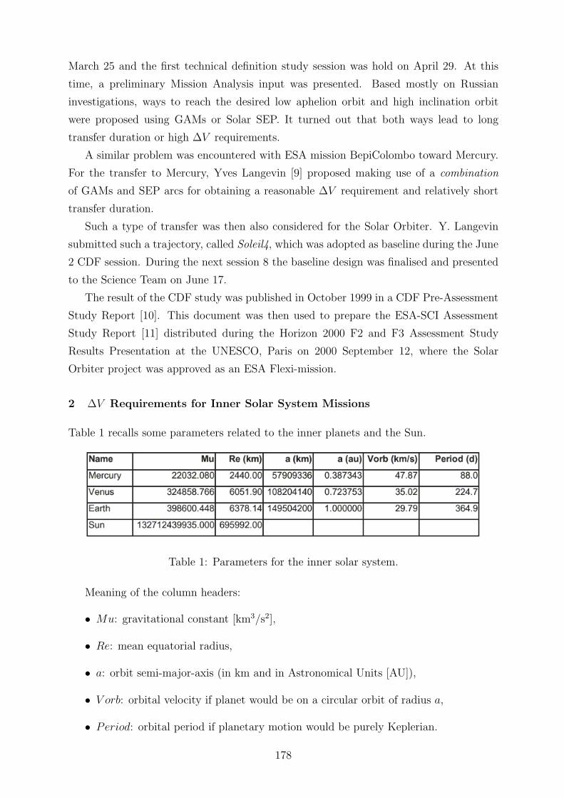
3.3 Inclination increase
GAM can also be used for increasing the inclination of the orbital plane. The maximum
potential of inclination increase for Mercury, Venus, Earth and Mars is given in Figure 1
in function of the in-coming infinite velocity. This diagram follows a formula given in
182
Inclination Change [deg]
0
2
4
6
8
10
12
14
0 4 8 12 16 20 24
Infinite velocity [km/s]
Mercury
Venus
Earth
Mars
Figure 1: (in colours). Maximum inclination increase function of the hyperbolic excess
velocity.
Ref. [8]. Results depend on the swing-by pericentre altitude: a value of 300 km was
selected in the cases presented here.
Figure 1 shows that, while Mercury has poor capabilities for inclination raise, Venus
and Earth do have some potential. However, for repetitive manoeuvres, an orbit of period
commensurable with the one of the planet has to be selected.
3.4 2012 launch
3.4.1 Trajectory design
The first step in the selection of a trajectory design is to define the sequence of swing-bys.
For every launch opportunity there is an optimum sequence. For the 2012 opportunity,
the following sequence reveals to be particularly attractive: E-V-E-E-V. It allows reaching
the desired target orbit with only 4 swing-bys instead of 5 (Section 3.1). However, the E-E
leg involves a 3:2 resonance orbit with the Earth lasting 2 years so that the total transfer
duration (close to 5 years) is not shorter than with more conventional GAM sequences as
discussed in Section 3.1.
The sum of the deterministic mid-course manoeuvres in this particular trajectory
design is very low (below 200 m/s). This value is so low that one may contemplate a
spacecraft design without orbit manoeuvre propulsion unit and entrust orbit manoeuvres
to the attitude thrusters.
3.4.2 Reference trajectory
3.4.2.1 Nominal mission: A reference trajectory for a launch on 2012-04-10 is proposed
183

Table 9: Summary of the 2012 launch ballistic reference trajectory.
here. It has been calculated by means of an optimisation program with a cost function
combining minimum deterministic ∆V for mid-course manoeuvres and minimum Earth
departure hyperbolic excess velocity. The trajectory is summarised on Table 9. Column
3 before the last indicates deterministic ∆V for Mid-Course Manoeuvre (MCM) between
2 consecutive GAMs. Actual ∆V will be slightly higher due to navigation errors. In
addition, an initial ∆V has to be added for removing the launchers injection error. The
two last columns indicate respectively the aphelion radius in AU and the perihelion radius
in Solar Radii [SR] of the orbit resulting from the event listed in column 3 (this is not the
radius at the time of the event). The minimum perihelion radius of 46 SR is reached after
the second Venus GAM on 2017-02-22. Earth and Venus swing-by pericentre altitudes
are all above 300 km (BepiColombo assumption, [5] Chap. 4).
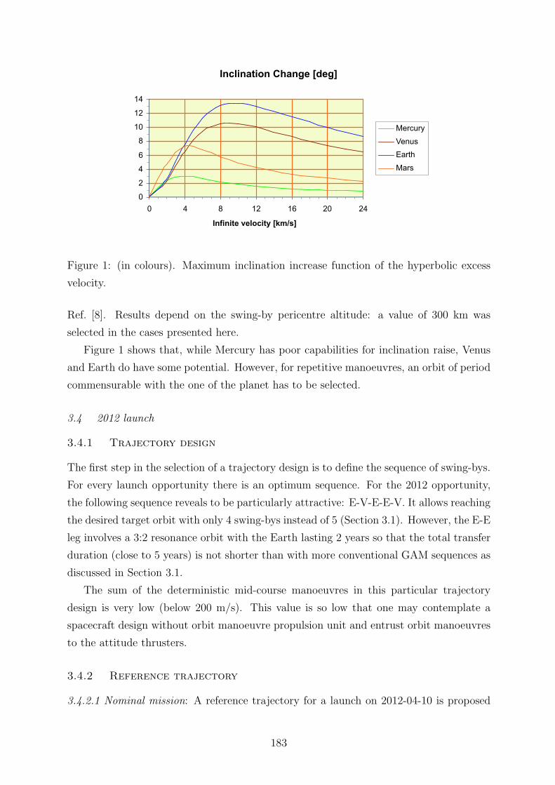
The end of the nominal mission is defined when the spacecraft leaves the orbit with
lowest perihelion radius, namely on 2018-05-17 (6 years after launch), when the second
Venus GAM on the resonance orbit is performed for inclination raise (causing a perihelion
radius raise). Definition of Cruise, Nominal, Observation and Extended phase of the
mission is visualised on Figure 2.
A projection of the trajectory during the nominal mission onto the ecliptic plane is
shown on Figure 3.
Figure 4 shows the trajectory during the cruise phase in a rotating coordinate system
such that the Earth-Sun line is fixed. Remarks on Figure 3 and Figure 4:
• The orbit of the terrestrial planets is shown by an orange (Mars), blue (Earth),
brown (Venus) and green line (Mercury).
184
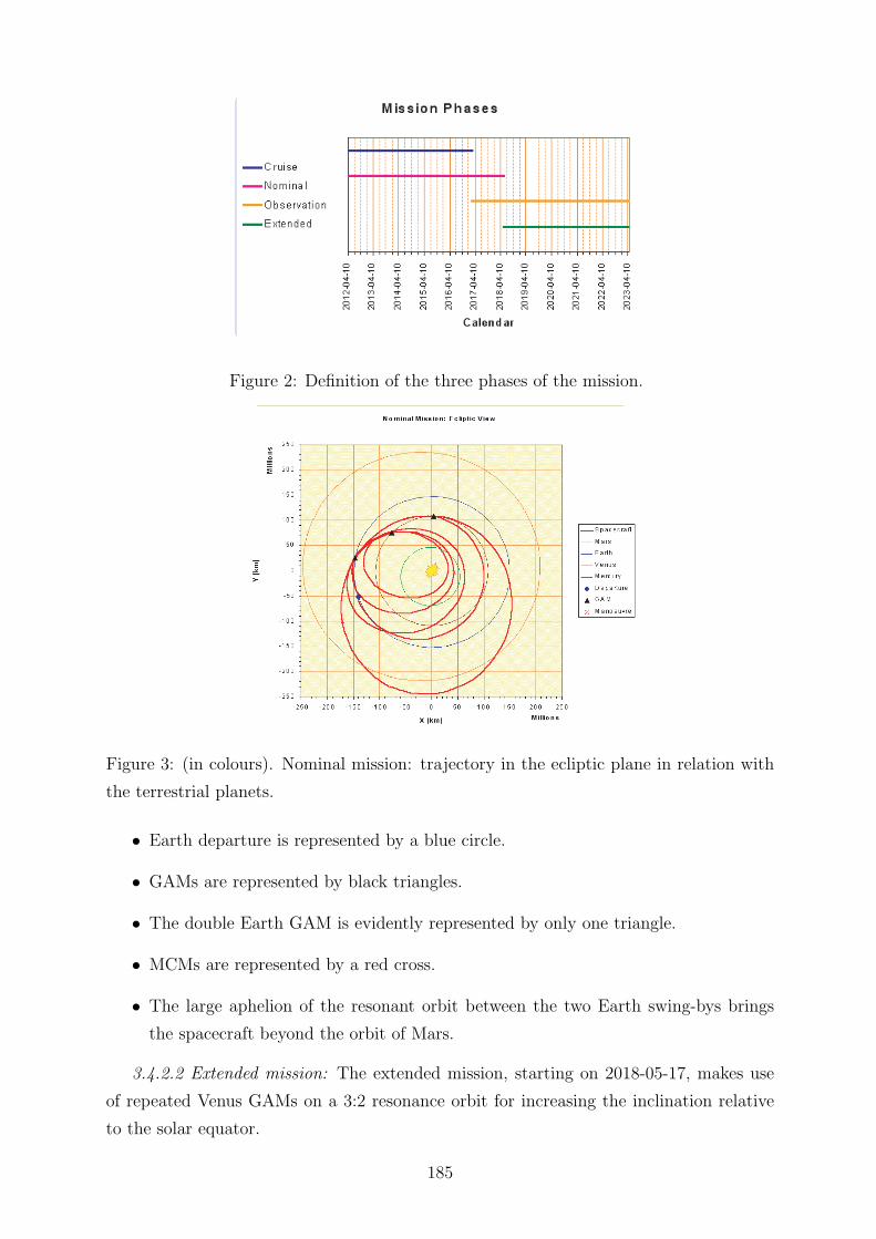
Figure 2: Definition of the three phases of the mission.
Figure 3: (in colours). Nominal mission: trajectory in the ecliptic plane in relation with
the terrestrial planets.
• Earth departure is represented by a blue circle.
• GAMs are represented by black triangles.
• The double Earth GAM is evidently represented by only one triangle.
• MCMs are represented by a red cross.
• The large aphelion of the resonant orbit between the two Earth swing-bys brings
the spacecraft beyond the orbit of Mars.
3.4.2.2 Extended mission: The extended mission, starting on 2018-05-17, makes use
of repeated Venus GAMs on a 3:2 resonance orbit for increasing the inclination relative
to the solar equator.
185

Nominal Mission: Ecliptic View
-250
-200
-150
-100
-50
0
50
100
150
200
250
-250 -200 -150 -100 -50 0 50 100 150 200 250
MillionsX [km]
Spacecraft
GAM
Manoeuvre
Figure 4: Cruise phase: trajectory in the ecliptic plane with Sun-Earth direction fixed
(x-axis).
The 3:2 resonance orbit of 150-day period is entered already during the second Venus
GAM on 2017-02-21, leading to the desired low perihelion orbit (46 SR). Three revolutions
(450 days) later the spacecraft experiences a Venus swing-by at the same orbital location.
Each GAM can modify the spacecraft orbit elements at the wishes of the mission designer,
which are:
• To keep on the resonant orbit for further GAMs.
• To increase the inclination relative to the solar equator.
• Not to further decrease the perihelion.
• To keep the swing-by altitude (the pericentre of the hyperbola) higher than a safe
distance (300 km).
For a given arrival velocity at the swing-by planet there are two free parameters
characterising a GAM. The most popular way to represent these parameters is making use
of the impact plane called also B-plane a plane normal to the hyperbolic arrival velocity
(parallel to the asymptote of the hyperbola) containing the centre of the planet. The two
Cartesian coordinates (ξ, η) in this plane, defining the impact point, are a representation
of the two free parameters. As each point in this plane corresponds to a specific departure
186

orbit, the post-swing-by orbit elements can be represented in the B-plane by level-line
curves. What needs to be represented in this analysis is
• the semi-major axis: the fixed value (a = 82580000 km = 0.552 AU) corresponding
to the 3:2 orbital period,
• the eccentricity, defining the perihelion radius,
• the inclination to the solar equator.
Such a B-plane representation for the second Venus GAM is shown on Figure 5:
• the solid black line represents the target semi-major axis (a = 0.552 AU),
• dashed red lines represent the eccentricity between 0.58 (inner curve) and 0.62 (outer
curve) by step of 0.1,
• dotted blue lines represent the inclination relative to the solar equator by steps of
2◦,
• solid light green circles represent the B-plane impact point altitude in km.
Figure 5: (in colours). Impact plane representation of the second Venus swing-by.
The axis coordinates (ξ, η) on Figure 5 is defined the following way:
187

Figure 6: (in colours). Impact plane representation of the third Venus swing-by.
• ξ-axis (z-axis, normal to B-plane) along arrival asymptote equivalent to infinite
velocity Varr∞
.
• η-axis (y-axis, ETA) along vector defined by V∞ × r, where r is the Sun-planet
radius vector
• ζ-axis (x-axis, DZETA) along direction of unit vector defined by η × ξ.
The selection of the impact point, subjected to the constraints mentioned here-above,
leads to a compromise represented by a point with approximate coordinates (-7030, 0)
km. The corresponding inclination on the solar equator and perihelion radius is listed in
Table 9.
The impact plane of the third Venus GAM is shown on Figure 6, where the eccentricity
is represented by red dashed lines between 0.54 (inner curve) and 0.6 (outer curve) by
step of 0.1. The selected impact point is approximately (-3950, 6750) km.
The impact plane of the fourth Venus GAM is shown on Figure 7, where the eccen-
tricity is represented by red dashed lines between 0.44 (inner curve) and 0.5 (outer curve)
by step of 0.1. The selected impact point is approximately (-5340, 4130) km.
The impact plane of the fifth Venus GAM is shown on Figure 8, where the eccentricity
is represented by red dashed lines between 0.36 (inner curve) and 0.42 (outer curve) by
step of 0.1. The selected impact point is approximately (-6340, 2500) km.
188
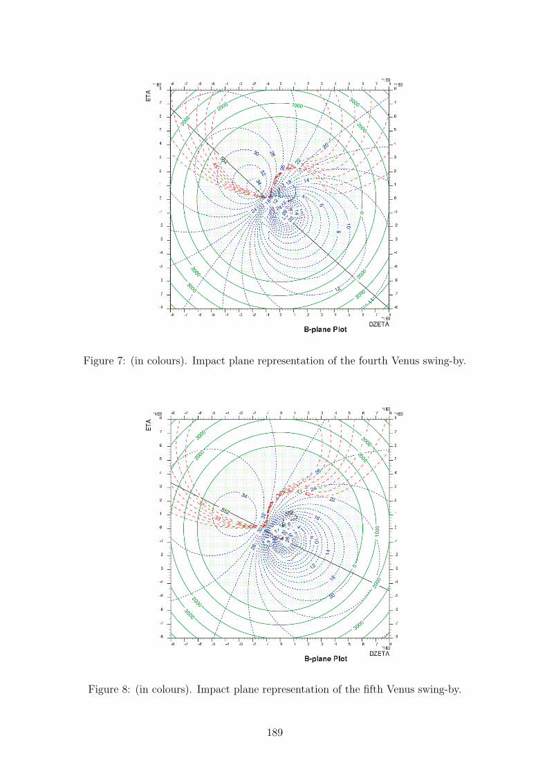
Figure 7: (in colours). Impact plane representation of the fourth Venus swing-by.
Figure 8: (in colours). Impact plane representation of the fifth Venus swing-by.
189

Figure 9: (in colours). Impact plane representation of the sixth Venus swing-by.
The impact plane of the sixth Venus GAM is shown on Figure 9, where the eccentricity
is represented by red dashed lines between 0.3 (inner curve) and 0.36 (outer curve) by
step of 0.1. The selected impact point is approximately (-6300, 790) km.
Further GAMs do not allow a further increase of the inclination. Therefore this sixth
GAM is the last one and it is no more necessary to aim for the 3:2 resonant orbit. The
selected point is aimed at a maximum inclination and minimum perihelion radius.
The increase of the inclination resulting from the successive GAMs is shown on Table 9,
where columns 5 and 6 give the inclination relative to the ecliptic and solar equatorial
plane respectively. After 4 successive GAMs, an inclination of 35◦ relative to the Sun
equator is reached, 9.7 years after launch. The trajectory during the extended mission is
illustrated in the ecliptic plane on Figure 10, in the plane X − Z normal to the ecliptic
on Figure 11 and in the plane Y − Z normal to the ecliptic on Figure 12.
3.4.3 Launch window
3.4.3.1 The 2012 Venus opportunity: The 2012 launch window for a Venus transfer is
shown on Figure 13. Solid lines show the Earth departure hyperbolic excess velocity and
dashed lines the declination of the departure hyperbolic asymptote. Figure 13 shows
clearly the two types of optimum transfers:
• Type 1 transfers (short transfers of the order of 3.5 months) have a Vinf below 3.6
190

Figure 10: Extended mission: trajectory in the ecliptic plane.
Figure 11: Extended mission: trajectory in the X − Z plane of the ecliptic referential
system.
191

Figure 12: Extended mission: trajectory in the Y − Z plane of the ecliptic referential
system.
Figure 13: 2012 Venus launch window. Solid line: hyperbolic excess velocity [m/s], dashed
line: declination of the asymptote.
192
km/s, a mid-March departure day and an early July arrival day.
• Type 2 transfers (long transfers of about 5.5 months with more than 180◦ transfer
angle) have a Vinf below 3.0 km/s, a late March departure day and a mid-September
arrival day.
3.4.3.2 The 2012 Solar Orbiter window: The definition of a launch window for in-
terplanetary flight is an iterative process. In principle the window can be arbitrarily
large, provided there is no limit in the launchers capability and ample ∆V available for
mid-course manoeuvres. Usually the iterative process converges toward a 2 to 4 weeks
window.
For a start, a standard 3-week window is assumed here. Optimum trajectories have
been calculated at various dates during the 2012 opportunity and a set of 21 consecutive
days where
• Earth departure hyperbolic excess velocity [Vinf],
• total deterministic mid-course ∆V is below a reasonable value is isolated.
In this preliminary window estimation, no consideration on the departure declination
of the asymptote has been included (for a low latitude launch pad, such as Kourou, this
may influence the launchers performance and therefore the definition of the window).
Optimal escape velocity and total expected deterministic ∆V for mid-course manoeuvres
during the nominal mission in terms of the launch date is shown on Figure 14. Giving
more weight to the escape velocity results in the following selection for a 3-week window:
• Window start/end: 2012 April 1/20.
• Maximum Vinf: 3.5 km/s.
• Maximum sum of deterministic mid-course manoeuvres: 166 m/s.
If during a later phase of the project (definition phase) spacecraft mass estimate in-
creases above the value associated with the launchers performance for this window, there
is a possibility to reduce the size of the window, reducing the maximum Vinf and thus
increasing the available launchers performance.
The proposed window is shown on Figure 13 (yellow rectangle). It is interesting to
notice that the window is not centered on the optimum window for a Venus transfer. This
results from the fact that the goal of the transfer is not just to arrive to Venus, but also
rather to have an optimum Venus arrival velocity vector for the GAM toward the Earth.
The selected arrival dates result from the overall trajectory optimisation program.
193

Figure 14: Required hyperbolic excess velocity and total deterministic ∆V for mid-course
manoeuvres during the nominal mission in terms of the launch date.
3.4.4 Auxiliary calculations
The distance from the spacecraft to the Sun, Venus and Earth during the mission is shown
on Figure 15, while the Sun-spacecraft-Earth angle is shown on Figure 16. This angle
should not be close to 0◦ or 180◦ before and during critical parts of the transfer such as
GAM and mid-course manoeuvres. This is verified.
Figure 15: (in colours). Distances spacecraft to Sun, Venus and Earth in million km.
Capability of the spacecraft to observe the Sun at high latitudes is shown on Figure 17,
where the solar latitude of the sub-spacecraft point in the Sun equatorial system is shown
in terms of the flight time. The same parameter is shown in terms of the distance of the
spacecraft to the Sun on Figure 18.
A scientific requirement is to be able to observe the Sun from a heliostationary point
of view. On an eccentric orbit, this is only possible along an arc around the perihelion, see
194
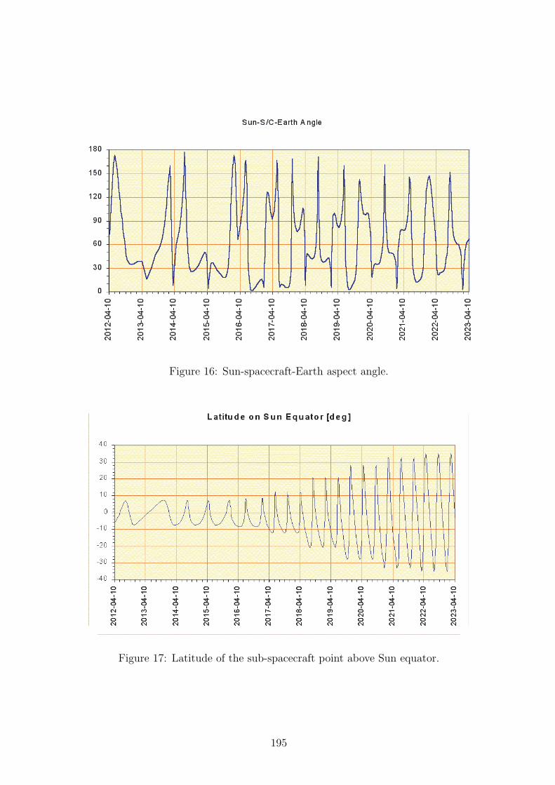
Figure 16: Sun-spacecraft-Earth aspect angle.
Figure 17: Latitude of the sub-spacecraft point above Sun equator.
195

Figure 18: Latitude of the sub-spacecraft point above Sun equator in terms of spacecraft
distance to Sun.
Table 10. It gives for all encountered perihelion during the mission the orbit angular rate
and angular rate relative to the solar rotation rate (14.18◦/day at the equator). None of
the rate reaches 0 but the low perihelion radius orbit between day 1779 and 2228 leads to
a relative rate of -1.9◦/day. The following Venus GAMs allow increasing the inclination
but unfortunately increase also the perihelion radius, decreasing therefore the orbit rate.
3.4.5 Mass budget
To the maximum deterministic ∆V budget indicated in Section 3.4.3.2 one has to add
the correction of the launcher injection error and provision for navigation uncertainties
correction and GAM preparation. If a Soyuz launcher with a Fregat upper stage is
considered, its dispersion is low and can be corrected by a manoeuvre performed around
10 days after launch at a maximum cost of 10 m/s (Mars Express, Ref. [4]). Navigation
errors and GAM preparation manoeuvres lead to a ∆V cost estimated to be about 35
m/s per leg between GAMs ([13]). A total of 8 GAMs are foreseen during the nominal
and extended mission, which leads to a maximum total navigation ∆V of 280 m/s. This
is probably a conservative figure, which may be revised downward after a detailed error
analysis.
Adding to this budget the maximum deterministic ∆V for mid-course manoeuvres
encountered in the launch window (166 m/s), one arrives to a total ∆V of 456 m/s.
Assuming a Soyuz/ST + Fregat launch from Baikonur (Chap. 6) with a maximum
196

Table 10: Orbit rate and rate relative to Sun rotation rate for every perihelion passage.
escape velocity of 3.5 km/s, the launchers performance is 1330 kg (Figure 31). To this
figure an adapter of 70 kg has to be subtracted.
Assuming, as proposed in the Trajectory Design Section (i.e. Section 3.4.1), using
only hydrazine attitude thrusters with a specific impulse of 220 s for orbit manoeuvres,
the corresponding propellant load is 240 kg, which leads to a spacecraft dry mass of 1020
kg. The ∆V allocation being conservative, there is no need to add propellant margin.
If a bi-liquid propulsion system with a specific impulse of 320 s is retained in the
spacecraft design, the propellant load is only 170 kg, leaving a spacecraft dry mass of
1090 kg.
According to Ref. [10], the spacecraft dry mass without SEP, cruise power system and
payload is 677 kg (including system margin and 20% overall mass margin). Adding to
this figure 24 kg of tankage for the hydrazine (10% of propellant mass), allowed payload
mass is 102067724 = 319 kg. This mass includes instrument margin and overall 20% mass
margin.
4 Solar Electric Propulsion
4.1 Characteristics of solar electric propulsion
In this Chapter, Solar Electric Propulsion (SEP) is assumed to be a non-impulsive thrust
characterized by
197

• Thrust in Newton.
• Specific impulse in seconds.
Other SEP characteristics (power, efficiency, etc.) are not considered here. In practice,
the magnitude of the thrust is less than 1 N while the specific impulse is 1600-2000 s
(plasma drive) or more (3000-4700 s for an ion drive).
For solar system cruise, the thrust depends on the power received by the Sun, therefore
on the distance to the Sun. The inverse square law is in theory applicable. However, for
practical reasons, it is recommended to select a slower increase, such as a power -1.7
law ([7]). However, when the distance to the Sun becomes small, the thermal stress is
becoming very high and the solar panels have to be inclined relative to the Sun direction.
This results in an empirical power law in terms of the heliocentric distance, such as the
one illustrated in Figure 19 in the case of GaAs solar arrays ([3]). Below 0.44 AU, solar
power can no more be increased and, at best, stays constant at 2.35 times the level at 1
AU.
Figure 19: Power law for GaAs solar cells with variable inclination relative to Sun direction
in terms of heliocentric distance in AU. Thrust proportional to the power is assumed here.
To have a first idea of the propellant and thrust time requirements, simple calculation
of some typical cases were performed assuming tangential thrust and fixed true anomaly
of start/end of thrust arc. Results of calculation are presented in form of Tables.
4.2 Perihelion reduction in the ecliptic
Starting from an Earth-Venus type transfer trajectory in the ecliptic, a perihelion reduc-
tion by SEP is investigated. In plane tangential thrust is performed between true anomaly
198

±20◦ around apogee (see Ref. [13]). Results are given in a form of a Table. Nominal thrust
at 1 AU, specific impulse and initial spacecraft mass are free input. The case with:
• thrust at 1 AU: 0.1 N,
• specific impulse: 3200 s,
• initial mass: 350 kg
is given here in Table 11. Meaning of the columns:
• Time (y): flight time between initial orbit and orbit with perihelion Rp,
• Nrev: number of revolution around the Sun during Time,
• Rp (Gm): perihelion radius in Gigameters (million of km),
• Rp (AU): perihelion radius in AU,
• Rp (Rs): perihelion radius in solar radius,
• M/M0: ratio between a spacecraft initial mass and final mass,
• M (kg): spacecraft final mass in kg,
• Thrust days: total thrusting time in days,
• Period (d): period of the final orbit in days,
• Vp (km/s): velocity at perihelion in km/s.
Table 11: Perihelion radius reduction by SEP at aphelion at 1 AU.
On top of the columns, input values are given in bold character, namely: the thrust at 1
AU (Thrust), specific impulse (Isp) and initial spacecraft mass (M0). The corresponding
199

mass flow (dM/dt) in kg/day is calculated. The initial aphelion height (1 AU) is also
given.
Results are scalable depending on the three free parameters (in bold character in the
sheet):
• Increase of thrust reduces the time and increases the mass flow.
• Increase of specific impulse decreases the mass flow, but not the time.
• Increase of initial mass increases the time and the mass flow.
4.3 Inclination increase
The major challenge of the Solar Orbiter mission is to reach a high inclination orbit.
Starting from a 156 × 40 solar radius orbit in the ecliptic, obtained for instance after a
series of gravity assist manoeuvres, an inclination change is calculated by vertical thrusting
at aphelion between true anomaly ±15◦ (see [13]). A particular case, where the three free
parameters are
• thrust at 1 AU: 0.1 N,
• specific impulse: 3200 s,
• initial mass: 350 kg
is shown on Table 12. Meaning of the columns is the same as in Table 11, except the last
column (Incl.) where the final inclination is shown.
Table 12: Inclination increase by SEP for a 1 × 0.19 AU orbit in the ecliptic plane.
4.4 Combined perihelion reduction and inclination increase
Inclination increase in Section 4.3 is most efficiently performed on an orbit with low peri-
helion. The perihelion reduction has to be therefore performed first. If it is also performed
200

by SEP, it is more efficient to combine the perihelion reduction and the inclination in-
crease. This can be achieved by selecting an inclined thrust direction. A suitable value
was found to be a declination of 55◦ on the ecliptic with the ecliptic component tangential
to the orbit.
The corresponding results are shown on Table 13.
Table 13: Combined perihelion radius reduction and inclination increase by SEP with an
aphelion at 1 AU.
4.5 Orbit circularization
If the orbit is close to the ecliptic plane, a partial circularization can be achieved by
gravity assist by Mercury. However, this takes a long time (several years). If the orbit
has a sizeable inclination to the ecliptic, gravity assist manoeuvres are becoming difficult
to obtain and use of SEP is more practical.
Circularization is achieved by thrusting at perihelion. Starting from the same 15640
solar radii orbit as in Section 4.3, a tangential thrust performed between ±45◦ around
perihelion reduces aphelion and achieves circularization. A certain gravity loss has to be
tolerated during the first years when eccentricity is high. Then, gravity loss decreases
during circularization and thrusting arc could even be increased for reducing the transfer
time. The result, in the particular case when
• thrust at 1 AU: 0.1 N,
• specific impulse: 3200 s,
• initial mass: 350 kg
is shown on Table 14.
201

Table 14: Aphelion radius reduction by SEP with a perihelion radius of 40 solar radii.
5 Gravity Assist Combined with Low Thrust Manoeuvres
5.1 Trajectory design
For a combined GAM + SEP mission toward the inner solar system, the following sequence
of GAMs has revealed to be optimum: E-V-E-V (BepiColombo [9]). SEP thrust phases
are inserted the following way:
• Shortly after launch to reduce launchers performance requirement.
• Between Venus and Earth GAM.
• Two or three thrust phases between Earth and Venus swing-by for optimal Venus
GAM leading to desired target orbit.
Acquisition of high inclination orbit with respect to solar equator is then accomplished
by a series of Venus GAMs on a 3:2 resonance orbit, as described in Section 3.4.2.2.
5.2 Lunar swing-by
To reduce requirements on the launcher performance, an Earth-to-Earth transfer prior to
the transfer to Venus can be inserted. Of course, this increases the cruise time by one
year. A further reduction of the launch energy can be achieved by adding a lunar GAM
helping injection into escape orbit. The lunar GAM provides enough energy to reach a
hyperbolic orbit.
The launch energy required for reaching the Moon on a 200×400000 km orbit amounts
to a C3 of 1.93 km2/s2. Corresponding Soyuz/ST performance is 2020 kg for a Baikonur
launch or 2230 kg for a launch from Kourou (Chap. 6). A low-thrust arc has to be
inserted close to aphelion of the Earth-to-Earth transfer producing a ∆V of 0.76 km/s
202
improving the Earth GA. The hyperbolic excess velocity obtained after the Earth GAM
is 3.94 km/s, allowing a short transfer to Venus (lower part of the diagram in Figure 13).
Soyuz/ST performance for directly targeting such a hyperbolic velocity would be 1180 kg
only. The benefit of the lunar swing-by (LSB) procedure is therefore considerable.
The interesting point in this LSB procedure is that the subsequent part of the cruise
phase is very similar to the direct launch. Therefore, in a first approximation, the LSB
can simply be added backward to the direct launch option.
In a direct launch, when the launcher does not provide the necessary 3.94 km/s for
the short transfer to Venus, a thrust arc is to be added shortly after launch for increasing
the orbital energy.
5.3 Reference trajectory
5.3.1 Nominal mission
A reference trajectory for a 2011-2012 launch is proposed here and summarised on Ta-
ble 15. This trajectory is based on the following assumptions:
• Direct injection option:
– An optimum balance between the use of the launchers injection capability
and the spacecraft on-board propulsion unit leads to the selection of an escape
velocity of 2.94 km/s to be provided by the launcher. Corresponding Soyuz/ST
performance is 1475 kg (Chap. 6).
– To provide for a launch window a certain performance margin is to be included.
BepiColombo mission analysis ([6]) has shown that escape energy requirement
along a 2-week launch window does not vary substantially. This is due to
the fact that the SEP phase following spacecraft separation from the launcher
allows partial compensation in the escape velocity requirement dependent on
the launch day at very small propellant cost. The analysis performed for Bepi-
Colombo in Ref. [1] shows that a margin of about 1.5% is sufficient to take
care of a 3-week window. This results in a usable Soyuz/ST performance of
1384 kg, where a 70 kg adapter has been subtracted ([1]).
• Lunar swing-by option:
– To reach the Moon, the spacecraft needs to be injected in a 200?400000 km
orbit. A launch from Baikonur is assumed and corresponding Soyuz/ST per-
formance is 2020 kg (Chap. 6).
– A launch window is achieved by launching in advance on the lunar transfer orbit
and waiting an integer number of revolutions until nominal lunar encounter
203

time, which has to occur at a specific day. If this encounter time is missed, the
mission is lost. The period of the lunar transfer orbit is about 11 days. This
means that a launch can be attempted every 11 days. A nominal plus 3-attempt
launch window is therefore 33 days long. Nominal launch day is 2010-12-29.
In contrast to the direct launch, there is no mass penalty associated with this
window.
• Moon swing-by minimum pericentre altitude is 200 km while Earth and Venus
swing-by pericentre altitudes are all above 300 km (following a BepiColombo as-
sumption, [1] Chap. 3).
• SEP is assumed to provide a constant thrust (about 0.2 N) with a specific impulse
of 4200 s.
• For the calculation of the mass budget, the following assumptions are made:
– An adapter mass of 70 kg is to be subtracted from the launchers performance.
– For the direct launch option, a 1.5% of the launchers performance is to be
subtracted for taking care of a 3-week launch window.
– The mass of the dry SEP system (including power module) is given by the
BepiColombo formula ([1] Section 3.1):
mSEP = 0.175 mS/C + 242 [kg]
where mS/C is the mass of the spacecraft at launch.
– The structural mass of the spacecraft (without SEP system and without pay-
load) is equal to the launch mass multiplied by 0.435. This crude figure comes
from [10] where a 677 kg structural spacecraft mass was launched with a Soyuz
on a 2.44 km/s escape orbit. Soyuz/ST performance for such a hyperbolic
excess velocity is 1555 kg, after having subtracted adapter mass and provision
for the launch window. The ratio 677/1555 ≈ 0.435 is taken here as a base for
the estimation of the spacecraft structural mass in terms of the mass of the
spacecraft at launch.
– During the extended mission, hydrazine thrusters are used for pre and post
GAM correction manoeuvres. ∆V usage for such manoeuvres is assumed to
be 35 m/s per GAM (Ref. [13]).
Remarks on Table 15:
• The first date in first column gives the latest launch date allowing reaching the
Moon for the LSB. To allow for 3 more launch attempts (at interval of 11 days)
along a one-month launch window, nominal launch date shall be on 2010-12-29.
204
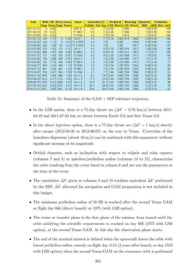
Table 15: Summary of the GAM + SEP reference trajectory.
• In the LSB option, there is a 75-day thrust arc (∆V = 0.76 km/s) between 2011-
04-19 and 2011-07-03 but no thrust between Earth GA and first Venus GA.
• In the direct injection option, there is a 77-day thrust arc (∆V = 1 km/s) shortly
after escape (2012-03-20 to 2012-06-05) on the way to Venus. Correction of the
launchers dispersion (about 10 m/s) can be combined with this manoeuvre without
significant increase of its magnitude.
• Orbital elements, such as inclination with respect to ecliptic and solar equator
(columns 7 and 8) or aphelion/perihelion radius (columns 14 to 15), characterise
the orbit resulting from the event listed in column 6 and are not the parameters at
the time of the event.
• The cumulative ∆V given in columns 9 and 10 totalises equivalent ∆V performed
by the SEP. ∆V allocated for navigation and GAM preparation is not included in
this budget.
• The minimum perihelion radius of 50 SR is reached after the second Venus GAM
at flight day 666 (direct launch) or 1075 (with LSB option).
• The cruise or transfer phase is the first phase of the mission, from launch until the
orbit satisfying the scientific requirements is reached on day 666 (1075 with LSB
option), at the second Venus GAM. At this day the observation phase starts.
• The end of the nominal mission is defined when the spacecraft leaves the orbit with
lowest perihelion radius, namely on flight day 1114 (3 years after launch, or day 1523
with LSB option) when the second Venus GAM on the resonance orbit is performed
205

for inclination raise (causing a perihelion radius raise). The rest of the mission is
called extended mission (Figure 20).
• During the last Venus GAM (# 6) an inclination increase is no more possible but
the perihelion can be again reduced from 76 to 52 SR.
Figure 20: Definition of the phases of the mission.
Trajectory optimisation leading to the results presented here has been checked by
an independent calculation performed with an alternate optimisation program. A good
agreement was found on the place and length of the thrust phases and the SEP propellant
mass figures were found to be about 10% lower with the alternate method. Therefore, it
is not necessary to add a margin to the SEP propellant consumption listed here.
A launch from Baikonur was assumed in the results displayed in Table 15. Launching
from Kourou (Section 0) does not change performance in escape orbit (direct launch op-
tion) but, according to STARSEM performance figures (Section 6.1), it does considerably
increase performance in elliptic and near-parabolic orbit. In the LSB option, performance
from Kourou in lunar transfer orbit is 2230 kg. Doing the same exercise as above, one
arrives at a very substantial final payload mass of 341 kg.
A projection of the nominal trajectory onto the ecliptic plane is shown on Figure 21.
On Figure 22 the cruise phase trajectory is shown in the ecliptic plane in a rotating coor-
dinate system with the Sun-Earth direction fixed. Remarks on Figure 21 and Figure 22:
• The orbit of the Earth and Venus is shown by a blue and brown line respectively.
• Earth departure is represented by a blue circle: dark blue for the LSB option and
light blue for the direct launch option.
206
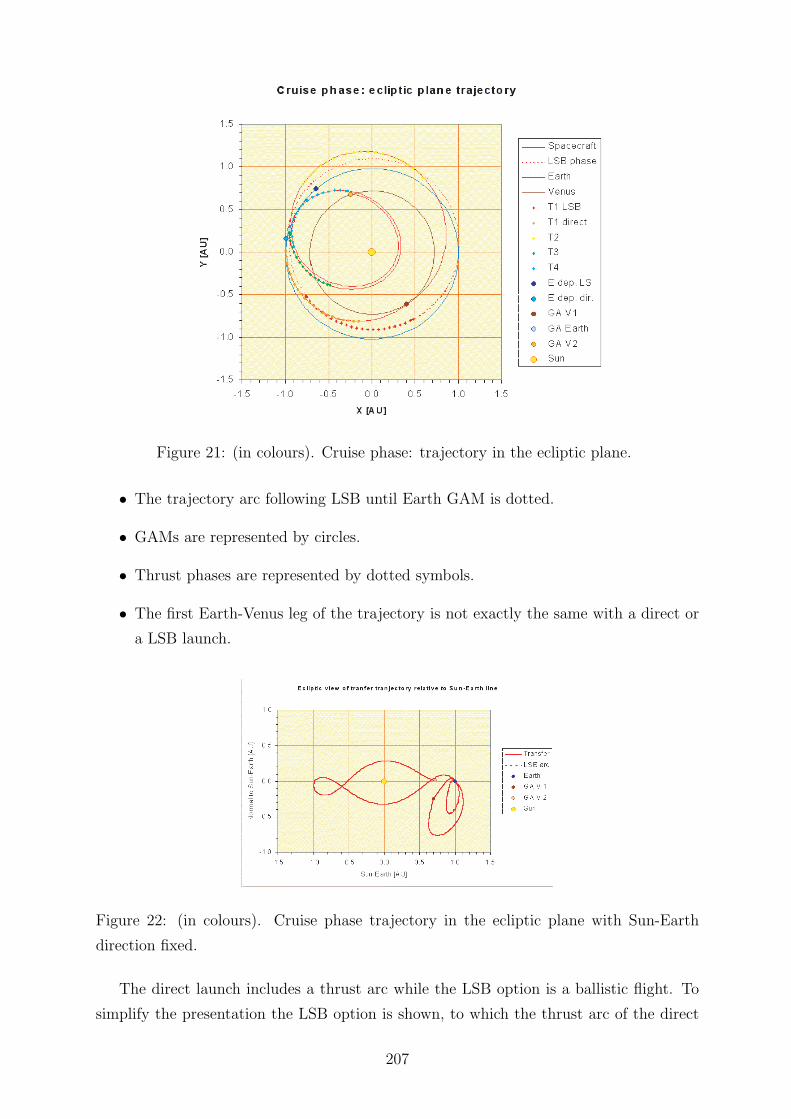
Figure 21: (in colours). Cruise phase: trajectory in the ecliptic plane.
• The trajectory arc following LSB until Earth GAM is dotted.
• GAMs are represented by circles.
• Thrust phases are represented by dotted symbols.
• The first Earth-Venus leg of the trajectory is not exactly the same with a direct or
a LSB launch.
Figure 22: (in colours). Cruise phase trajectory in the ecliptic plane with Sun-Earth
direction fixed.
The direct launch includes a thrust arc while the LSB option is a ballistic flight. To
simplify the presentation the LSB option is shown, to which the thrust arc of the direct
207
launch option has been superimposed. After the first Venus GAM the two trajectories
are nearly identical.
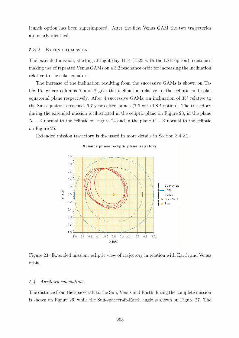
5.3.2 Extended mission
The extended mission, starting at flight day 1114 (1523 with the LSB option), continues
making use of repeated Venus GAMs on a 3:2 resonance orbit for increasing the inclination
relative to the solar equator.
The increase of the inclination resulting from the successive GAMs is shown on Ta-
ble 15, where columns 7 and 8 give the inclination relative to the ecliptic and solar
equatorial plane respectively. After 4 successive GAMs, an inclination of 35◦ relative to
the Sun equator is reached, 6.7 years after launch (7.9 with LSB option). The trajectory
during the extended mission is illustrated in the ecliptic plane on Figure 23, in the plane
X − Z normal to the ecliptic on Figure 24 and in the plane Y − Z normal to the ecliptic
on Figure 25.
Extended mission trajectory is discussed in more details in Section 3.4.2.2.
Figure 23: Extended mission: ecliptic view of trajectory in relation with Earth and Venus
orbit.
5.4 Auxiliary calculations
The distance from the spacecraft to the Sun, Venus and Earth during the complete mission
is shown on Figure 26, while the Sun-spacecraft-Earth angle is shown on Figure 27. The
208

Figure 24: Extended mission: trajectory in the plane X −Z normal to the ecliptic plane.
Figure 25: Extended mission: trajectory in the plane Y −Z normal to the ecliptic plane.
Sun-spacecraft-Earth angle should not be close to 0◦ or 180◦ before and during critical
parts of the transfer such as GAM and mid-course manoeuvres. This is verified.
Capability of the spacecraft to observe the Sun at high latitudes is shown on Figure 28,
where the solar latitude of the sub-spacecraft point in the Sun equatorial system is shown
in terms of the flight time. The same parameter is shown in terms of the distance of the
spacecraft to the Sun on Figure 29.
A scientific requirement is to be able to observe the Sun from a heliostationary point
of view. On an eccentric orbit, this is only possible along an arc around the perihelion.
Table 16 gives for all encountered perihelions during the mission the orbit angular rate
and angular rate relative to the solar rotation rate (14.18◦/day at the equator). None of
the rates reaches 0 but the low perihelion radius orbit between day 666 and 1114 leads to a
relative rate of only -3.1◦/day. The following Venus GAMs allow increasing the inclination
209

Figure 26: (in colours). Distances spacecraft to Sun, Venus and Earth in AU.
Figure 27: Sun-spacecraft-Earth aspect angle (degree, left scale) and solar radiation inte-
grated doses (right scale).
210

Solar latitude [deg]
-40
-30
-20
-10
0
10
20
30
40
Figure 28: Solar latitude of sub-spacecraft point in the Sun equatorial system with respect
to flight time.
Figure 29: Solar latitude of sub-spacecraft point in the Sun equatorial system with respect
to the distance Sun-spacecraft.
but unfortunately increase also the perihelion radius, decreasing therefore the orbit rate.
Finally, the solar radiation integrated doses is displayed on Figure 30 as function of
the flight time for the case of a direct and LSB transfer. The solar radiation integrated
doses is a non-dimensional figure defined as the solar radiation doses normalised at 1 AU
along a unit of time divided by the flight time. It is proportional to the total (cumulated)
doses of solar radiation received by the spacecraft during the flight.
Figure 30 shows that, for a given flight time, this cumulative figure is higher for a
direct transfer than for the LSB option. This reflects the fact that in case of a LSB the
preliminary Earth-Earth leg goes outside the 1 AU radius and contributes little to the
total doses.
211
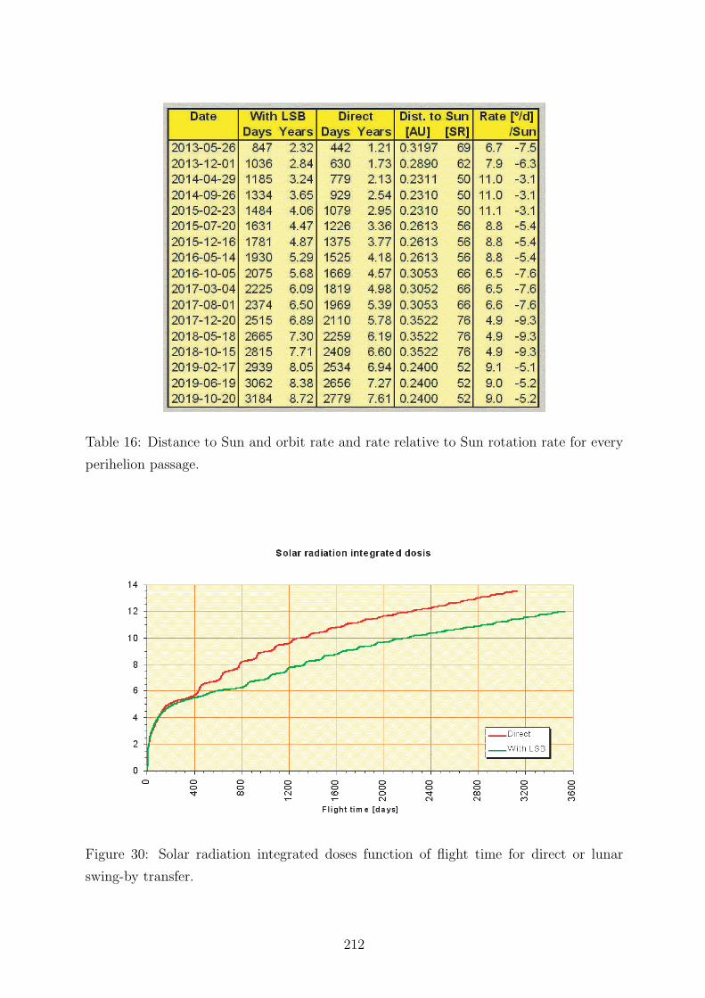
Table 16: Distance to Sun and orbit rate and rate relative to Sun rotation rate for every
perihelion passage.
Figure 30: Solar radiation integrated doses function of flight time for direct or lunar
swing-by transfer.
212
5.5 Navigation aspect
Navigation aspect of missions including low-thrust phases is still under investigation. A
recent study (Ref. [2]) shows that navigation accuracy is very much dependent on the
assumptions on the SEP parameters. As little experience is yet available on such param-
eters, it is too early to assess accuracy of the low-thrust phases of the flight. However, it
is expected that propellant for navigation will not exceed the 10% margin taken here on
the SEP propellant budget.
For a ballistic mission, a series of manoeuvres has to be scheduled before and after
each GAM. In Section 3.4.5 a provision of 35 m/s was foreseen for each GAM preparation
and correction.
6 Launchers Performance
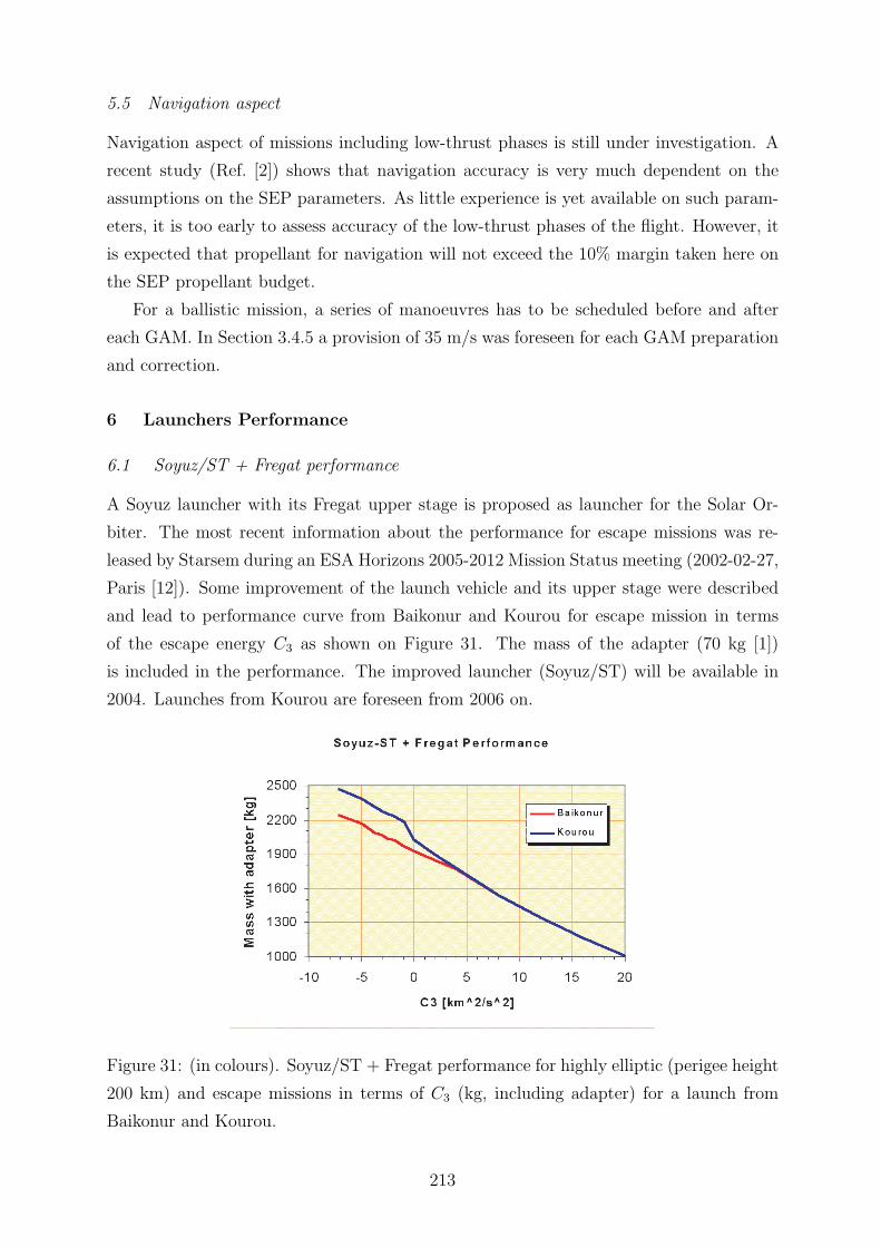
6.1 Soyuz/ST + Fregat performance
A Soyuz launcher with its Fregat upper stage is proposed as launcher for the Solar Or-
biter. The most recent information about the performance for escape missions was re-
leased by Starsem during an ESA Horizons 2005-2012 Mission Status meeting (2002-02-27,
Paris [12]). Some improvement of the launch vehicle and its upper stage were described
and lead to performance curve from Baikonur and Kourou for escape mission in terms
of the escape energy C3 as shown on Figure 31. The mass of the adapter (70 kg [1])
is included in the performance. The improved launcher (Soyuz/ST) will be available in
2004. Launches from Kourou are foreseen from 2006 on.
Figure 31: (in colours). Soyuz/ST + Fregat performance for highly elliptic (perigee height
200 km) and escape missions in terms of C3 (kg, including adapter) for a launch from
Baikonur and Kourou.
213
In a diagram mass versus C3 the performance curve is nearly linear. By extending
the line toward negative values of C3, performance for highly elliptic orbits can also be
shown on the same diagram for a given perigee height hp (usually 200 km). The relation
between C3 and apogee height ha is the following
C3 = −2µE
ha + hp + 2RE
where µE is the Earth gravitational constant (398600.448 km3/s2) and RE the mean Earth
equatorial radius (6378.14 km).
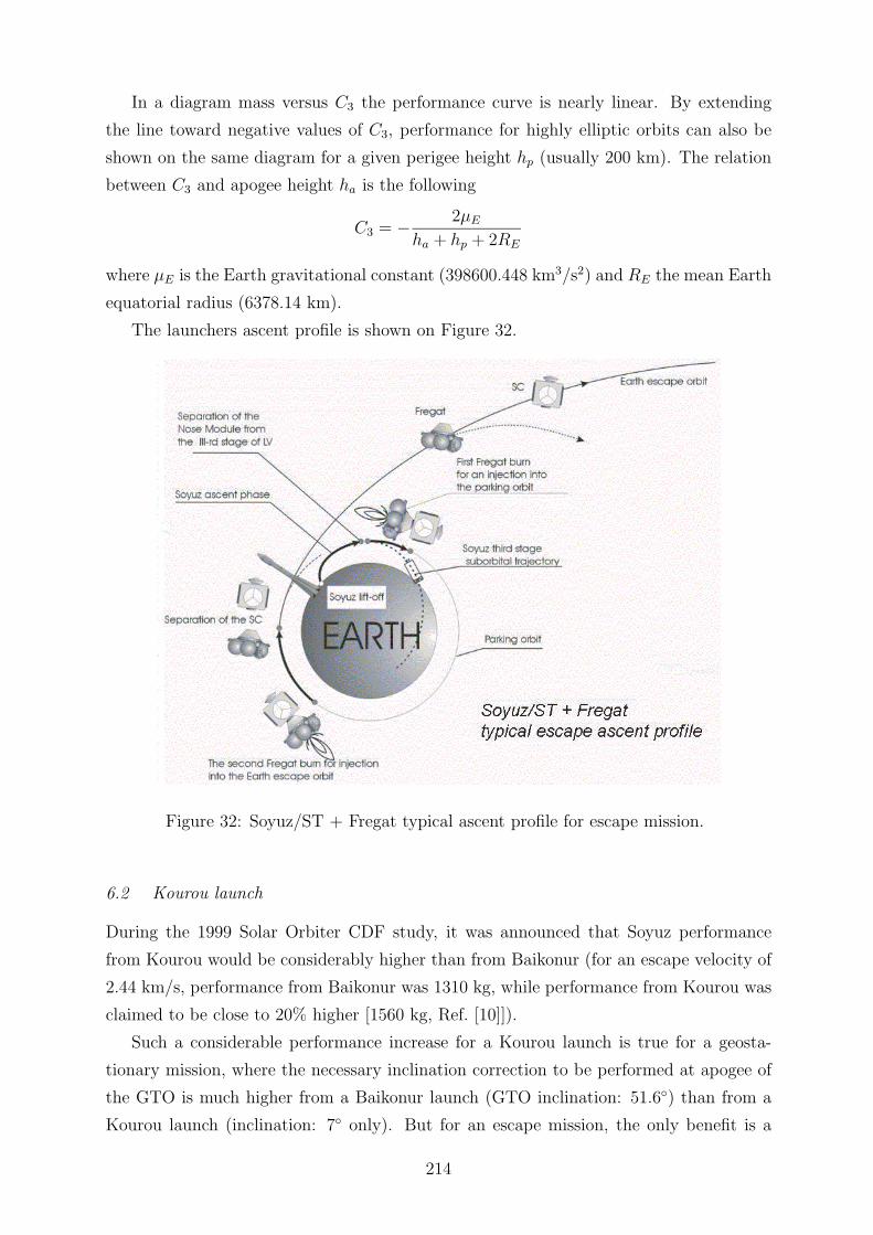
The launchers ascent profile is shown on Figure 32.
Figure 32: Soyuz/ST + Fregat typical ascent profile for escape mission.
6.2 Kourou launch
During the 1999 Solar Orbiter CDF study, it was announced that Soyuz performance
from Kourou would be considerably higher than from Baikonur (for an escape velocity of
2.44 km/s, performance from Baikonur was 1310 kg, while performance from Kourou was
claimed to be close to 20% higher [1560 kg, Ref. [10]]).
Such a considerable performance increase for a Kourou launch is true for a geosta-
tionary mission, where the necessary inclination correction to be performed at apogee of
the GTO is much higher from a Baikonur launch (GTO inclination: 51.6◦) than from a
Kourou launch (inclination: 7◦ only). But for an escape mission, the only benefit is a
214

higher velocity push due to the Earth rotation at a near-equatorial launch site. The ∆V
added by the Earth rotation is equal to
∆VE = ωE RE cos `,
where ωE is the Earth rotation rate (360.986◦/day), RE the Earth equatorial radius and `
the latitude of the launch site (5.2◦ for Kourou and 45.6◦ for Baikonur). The contribution
by the Earth rotation is thus 0.463 km/s from Kourou and 0.325 km/s from Baikonur,
assuming perfect due east launches. The difference is 138 m/s.
Actually the difference is less because the inclination of the parking orbit for a Baikonur
launch allows reaching any declination of the asymptote encountered in interplanetary
flight mission, while a Kourou launch is penalised in case the target declination is high.
For instance, the Solar Orbiter launch declination can reach 20◦ (Figure 13), obliging the
launcher from Kourou to inject into a 20◦ orbit. Experience with Ariane launches show
that decrease of performance when aiming to inclined orbits is considerable, far more than
Earth rotation contribution can justify. The reason is due to the constraint on the first
stage ground track not to hit populated areas. Such a constraint will for sure be also
applicable to Soyuz launches and make inclined target orbit unattractive.
The Ref. [12] performance curve (Figure 31) shows indeed that Kourou offers a per-
formance advantage only for escape velocities below 2 km/s, but this advantage vanishes
for higher escape velocities.
In conclusion, for the Solar Orbiter mission (direct launch option), where an escape
velocity of 2.5 to 4 km/s is needed (C3 from 6.3 to 16 km2/s2), there will be no advantage
of a Kourou launch. Baseline is therefore a Baikonur launch. (It turns fortuitously out
that the performance of the improved Soyuz from Baikonur [1650 kg for an escape velocity
of 2.44 km/s] is superior to the old optimistic performance from Kourou [1560 kg]).
In case of a LSB, where the spacecraft has to be injected into a high eccentricity elliptic
orbit, Figure 31 shows a substantial increase of performance for orbit of inclination smaller
than 28◦. However such performance looks to be very optimistic and needs to be confirmed
by the launch authority before using it for mission design.
7 Conclusion
The Solar Orbiter mission is composed of three main parts:
1. Launch and cruise phase for acquisition of the observation orbit.
2. Observation phase, when scientific requirements for solar observation are satisfied.
3. Extended mission, when the inclination of the orbit is raised.
215
The nominal mission is composed of the cruise and observation phase.
Launcher: a Soyuz/ST with a Fregat upper stage is proposed with launch from
Baikonur or Kourou.
Cruise phase, two options:
1. Ballistic cruise with GAMs with Venus and Earth and small impulsive mid-course
manoeuvres.
2. Use of SEP combined with GAMs.
In option 1, a 2012 launch in a 3-week window between April 1 and April 20 is proposed
with a required escape velocity of 3.5 km/s. Launchers performance is 1330 kg minus 70
kg for the adapter. Duration of the cruise phase is 4.8 years. ∆V for removing the
launchers dispersions (10 m/s), mid-course manoeuvres and preparation/correction of 4
GAMs amounts to a total of 316 m/s.
In option 2, a launch with an escape velocity of 2.94 km/s is optimum, corresponding
to a launchers performance of 1475 kg minus 70 kg for the adapter and 21 kg for providing
for a 3-week long launch window. During the cruise phase (1.85 y), not more than 118 kg
of propellant will be spent with the SEP unit. At the end of the cruise phase, the SEP
and its power unit (484 kg) will be ejected.
To reduce launchers performance requirement, an extra phase can be added in option
2: instead of launching directly into escape orbit, a lunar swing-by is performed allowing
to inject into an orbit encountering the Earth about one year later. This procedure, which
increases cruise duration by 443 days (taking into account a one-month launch window
allowing for 4 launch attempts on the lunar transfer orbit), allows increasing launch mass
by 566 kg. According to STARSEM performance in elliptical orbits for a Soyuz/ST launch
from Kourou, the launch mass increase can even reach 776 kg (TBC). In this LSB option,
nominal launch day is 2010-12-29.
In both options, the inclination raise will be performed during the extended mission
(duration: 3.7 y until a 35◦ inclined orbit is reached) by a sequence of 4 Venus GAMs
obtained by selecting a 3:2 resonant orbit with Venus. Preparation/correction of these
GAMs contributes to an additional 140 m/s.
Mass and mission phase duration are summarised in Table 17, where indicated masses
include system margin and an overall 20% margin. The mass figures on Table 17 are
preliminary figures based on rather crude assumptions on spacecraft structural mass and
solar electric propulsion system mass.
216

Table 17: Mass budget and mission phase duration for the ballistic and SEP cruise options
including direct launch and LSB from Baikonur and Kourou.
Acknowledgments
This paper is an extended version of an invited talk given at the Jornadas de Trabajo
en Mecanica Celeste, Senorıo de Bertiz, Navarra, Spain, in July 2003. Partial support
for participating in the Jornadas was given by Project # BFM2002-03157 of Ministerio
de Ciencia y Tecnologıa (Spain) and Project Resolucion 92/2002 of Departamento de
Educacion y Cultura, Gobierno de Navarra (Spain).
References
[1] Campagnola, S., Corral, C., Jehn, R. and Yanez, A.: 2003, BepiColombo Mercury
Cornerstone Mission Analysis: Inputs for the Reassessment Phase of the Definition
Study, draft 2.3, MAO WP 452, ESA-ESOC.
[2] Cano, J. L. and Bello, M.: 2002, Study on Feasibility of Solar Electric Powered Fly-bys,
ESA Contract No. 15760/01/D/HK, Hand-out of final presentation.
[3] Colangelo, G.: 1999, Preliminary Study for the System Thermal Design of the ESA
Solar Orbiter, viewgraph presentation to CesaR, ESA-ESTEC.
[4] Hechler, M. and Yanez, A.: 2001, ‘Mars Express orbit design’, IAF-01-A.1.06, 52nd
International Astronautical Congress 2001, Toulouse.
[5] Katzkowski, M., Corral, C., Jehn, R., Pellon, J. L., Landgraf, M., Khan, M., Yanez,
A. and Biesbroek, R.: 2002, BepiColombo Mercury Cornerstone Mission Analysis:
Input to the Definition Study, MAS WP432, ESA-ESOC.
217

[6] Katzkowski, M., Jehn, R. and Campagnola, S.: 2003, BepiColombo Mercury Cor-
nerstone Mission Analysis: Trajectory and Recovery Options, MAO WP 443, ESA-
ESOC.
[7] Konstantinov, M. and Fedotov, G.: 1997, ‘Estimation of an opportunity of Mercury
Mission with use of solar electric propulsion’, IAF-97-V.2.09, 48th International As-
tronautical Congress 1997, Turin.
[8] Labunsky, A. V., Papkov, O. V. and Sukhanov, K. G.: 1998, Multiple Gravity Assist
Interplanetary Trajectories, Earth Space Institute Book Series, Overseas Publ. Ass.,
Gordon and Breach Science Publications, Amsterdam.
[9] Langevin, Y.: 1999, ‘Chemical and solar electric propulsion options for a Mercury
cornerstone mission’, IAF-99-A.2.04, 50th International Astronautical Congress 1999,
Amsterdam.
[10] Solar Orbiter: 1999, Solar Orbiter Pre-Assessment Study Report, ESA CDF-02(A).
[11] Solar Orbiter: 2000, Solar Orbiter, a High-Resolution Mission to the Sun and Inner
Heliosphere, Assessment Study Report, ESA-SCI(2000) 6.
[12] Soyuz for Exploration Missions: 2002, Presentation to ESA/Astrium, Meeting ESA
Horizons Mission Status 2005-2012 and Soyuz, ESA-HQ, Paris.
[13] Sukhanov, A. A.: 1998, ‘Close approach to Sun using gravity assists of the inner
planets’, AAS 98, 389.
218