Embed Size (px)
Citation preview

1
Training: Often the Missing Link in Using
NDT Methods
By N. J. Carino
Synopsis: Nondestructive test (NDT) methods are indirect methods that rely on the interactions of some type of
mechanical or electromagnetic radiation with internal irregularities. Differences in response are used as indicators of
the presence of these irregularities. Often the underlying physics are complex and not the type of information that
most civil engineering students have studied, other than in basic physics courses. Yet civil engineers are called upon
often to evaluate structures using various types of advanced NDT methods. Successful application of these advanced
methods requires that persons taking the data and analyzing the data have a good understanding of the principles of
the methods, how to set up data acquisition parameters for optimum results, and how to interpret recorded data. This
requires investing resources in training, which is too often neglected because of budgeting or scheduling constraints.
Lack of training, can lead a user to arrive at incorrect conclusions from the NDT survey, which will cast a negative
image on the NDT method. Thus when planning on acquiring NDT equipment, the budget should include sufficient
funding for proper training. The benefits will outweigh the initial cost. This paper uses the impact-echo method as
an example to illustrate the kind of basic information that should be understood by all members of the team
conducting an evaluation using this method. The topics covered include: basic principles of stress-wave propagation
and reflection; the vibrational response of plate-like structures and prismatic members; frequency domain analysis of
waveforms; frequency content impact force; selection of data acquisition parameters; and minimum detectable flaw
size.
Keywords: amplitude spectrum, contact time, impact-echo method, frequency analysis, nondestructive testing, P-
wave, reflection, stress-wave propagation.
2
ACI and ASTM Fellow, Dr. Nicholas J. Carino is a consultant in Chagrin Falls, OH, USA. He retired from his
position as a research structural engineer at the National Institute of Standards and Technology after 25 years of
service. He has been an active member of ACI and ASTM for over 30 years and has held numerous leadership
positions in both organizations. He is the recipient of many awards in recognition of contributions to research and
standards-development. He is widely known for his work on nondestructive testing of concrete, and is a graduate of
Cornell University.
INTRODUCTION
Visual inspection remains the most versatile and powerful nondestructive test (NDT) method for evaluating the
condition of a concrete structure. With adequate experience and knowledge about structural behavior and
deterioration mechanisms, the inspecting engineer can learn a lot about the condition of a structure. They key phrase
is "adequate experience and knowledge." The engineer requires training to distinguish between features that are to
be expected and those that are not expected and are, therefore, indicators of abnormal behavior. For example, narrow
flexural cracks are to be expected in a reinforced concrete member, but wide cracks are not. If wide cracks are
observed, are they of concern for reasons other than aesthetics?
In visual inspection, the engineer is relying on the interaction of light reflection with the concrete surface and the
brain's ability to translate the received reflected light into an image that can be analyzed. While visual inspection is
powerful, it suffers from the obvious limitation that one can only obverse surfaces that are within view. So, other
methods are needed to "look" into the concrete. Over the years, several different approaches have been developed to
supplement visual inspection by gaining additional information about conditions below the surface. These methods
are based on interactions of the irregularities within a concrete member and some other physical process. The types
of "physical processes" that have been found successful include stress-wave propagation and electromagnetic wave
propagation (ACI 228.2R). They are "indirect methods" and the evaluation engineer needs to have an understanding
of the "basic physics" involved in each of the different methods that allow one to infer what the conditions are below
the surface. Most evaluation engineers have backgrounds in civil engineering, some with specialization in structural
engineering, geotechnical engineering, or construction materials. In most cases, formal undergraduate training does
not include specialized courses in NDT methods. This makes it mandatory that engineers obtain the necessary
training before attempting to use these methods.
The electromagnetic spectrum offers several opportunities to supplement the information obtained from the visual
portion of the spectrum. For example, by using short-wavelength penetrating radiation, such as x-rays and gamma
rays, we can obtain radiographs of the internal structure. These methods, however, require the extensive safety
measures to prevent harmful radiation exposure to personnel. In the infrared region of the spectrum, we can use
variations of surface temperature (under conditions of heat flow) as indicators of the presence of near-surface
irregularities that interfere with heat flow into or out of the member. With radiation in the microwave region, such as
used for ground penetrating radar (GPR), we can look into concrete by monitoring the nature of reflected pulses of
low-energy, electromagnetic radiation. Successful use of GPR requires an understanding of how the pulses emitted
by the antenna interact with different materials within the concrete, especially embedded metal objects.
There are many NDT methods based on stress-wave propagation that have proven to be capable of providing
information amount the condition of concrete members. These include methods based on measuring resonant
frequency, measuring the speed of stress pulses transmitted through the concrete, and monitoring stress waves
reflected from internal irregularities. In general, the principles of stress-wave methods are easier to grasp than are
the principles of methods based on electromagnetic radiation because of our experiences with sound waves. Also,
stress wave propagation in a solid is governed by the density and elastic properties of the solid, which are familiar to
civil engineers.
Tapping an object and listening to the resulting sound is one of the oldest forms of NDT based on stress-wave
propagation. This is essentially a resonance type of test where the initial impact leads to resonant vibrations at
different frequencies within the audible range (20 Hz to 20 kHz). Changes in these frequencies are indicators of

3
differences in the structure near the impact location. This method has been standardized by ASTM as Practice
D4580 for locating corrosion induced delamination in concrete bridge decks. The impact can be by a hammer, a
steel rod, several shorts length of chain attached to a bar, or a bicycle chain sprocket. The last approach allows rapid
testing of surfaces in any orientation. Two sprockets are attached to a handle, and the sprockets are rolled over the
surface. When the sprockets are rolled over a solid region, the tapping produces a high-pitched sound, but when they
roll over a delaminated region, a low-pitched rattle sound is heard. This "sounding" method has obvious limitations:
it cannot detect deep defects and the results depend on the experience of the operator to distinguish the different
sounds.
The limitations of "sounding" have led to the development of several other test methods based on stress-wave
propagation. These include ultrasonic pulse velocity, seismic-echo, impulse-response, impact-echo, pulse-echo
(pitch-catch method), and spectral analysis of surface waves (ACI 228.2R, Carino 2004). Again, successful
application of these methods requires that individuals who perform the tests and analyze the results have a good
understanding of the underlying physics, the inherent limitations of the method, how to set up the instrumentation,
and how to interpret the results. Often, the tests on concrete structures are performed by technicians who may have
been trained on how to acquire data with a particular instrument. Unless a technician is also trained in the underlying
principles of the method, that individual may not be able to recognize invalid data because of testing conditions.
Often, an investigating organization will purchase an advanced NDT system, but will choose not to invest additional
resources for the necessary training. The system may then be used on a major project and, because of the lack of
training, the conclusions from the NDT survey may not agree with the results of limited invasive probing. Two
things may happen: the investigator looses credibility and, more importantly, the test method looses credibility. The
latter is particularly important because it may cast doubt on the applicability of a method that has been well-
researched and is reliable when used correctly. A technically sound method can be discredited falsely when used by
an incompetent individual. A lot of effort is needed subsequently to restore the credibility of the method. Therefore,
persons planning on acquiring advanced NDT systems should include training as part of the initial cost. The
investment will pay for itself in repeat business as the investigator develops a proven track record of successful
projects.
Ideally, there should be a third-party certification program for providers of NDT services for concrete structures. At
this time (2009), however, no such program exists. ACI Committee 228 has a task group to address NDT
certification for in-place strength tests and advanced NDT methods, but a recommended course of action has not yet
been developed. A barrier to the development of a program is simple economics. The demand for NDT certification
is not at the same level as the demand for certification in the usual acceptance test methods. In the absence of a
third-party certification program, it is up to the investigating agencies to institute internal certification programs.
The impact-echo method will be used as an example to illustrate the kind of information that should be familiar to a
evaluation engineer. This information can be separated into three areas:
• The key principles that form the foundation of the method;
• The significance of the data acquisition parameter and testing variables;
• How to plan for the field investigation;
• Data interpretation and field verification.
These generic topics are applicable to any of the advanced NDT methods that have been mentioned.
CASE STUDY—The Impact-Echo Method
Overview
Figure 1 is a schematic of the impact echo method, which is based on using a short duration mechanical impact to
generate stress waves and a transducer to monitor the surface displacement due to the arrival of direct and reflected
stress waves. The use of mechanical impact provides a versatile method for introducing a much higher amount of
energy than is possible with an electrical transducer. The impact produces a force-time history that can be
approximated as a half-cycle sine curve. The duration of the impact is called the contact time and has to be chosen

4
carefully. The receiver measures displacement normal to the surface, and the displacement history is recorded and
stored as a time-domain waveform as shown on the top right side of Fig. 1. As will be explained, the energy from the
impact causes the test element to vibrate at a characteristic frequency or frequencies, and these frequencies provide
information about the integrity of the element. A key feature of the data analysis method is the transformation of the
time-domain waveform into the amplitude spectrum, which will identify the resonant frequencies that are embedded
in the waveform. The user needs to understand how to interpret these frequencies. The following sections address
the basic information that should be understood by users of the impact-echo method. A summary of the development
of the impact-echo method and a comprehensive treatment of impact-echo testing are available and should be read
by anyone planning on using the method (Sansalone 1997; Sansalone and Streett 1997)
Figure 1—Schematic of the impact-echo method
Stress waves due to impact
When a solid is struck at a point, the disturbance propagates away from the impact point as three types of stress
waves. The P-wave and the S-wave propagate into the solid along expanding spherical wavefronts, and the R-wave
travels away from the impact along the "near-surface" region (this is similar to the ripples created when a rock is
thrown into a pond). The P-wave travels at the fastest speed and is associated with a normal stress. When the P-wave
passes by a given point, a particle vibrates parallel to the direction of propagation, that is, along the radius drawn
from the impact point to the location of the particle (this line is called a ray path by analogy to a light ray). The S-
wave travels at a slower speed and is associated with a shearing stress. When the S-wave passes by a point, the
particles vibrate perpendicular to the direction of wave propagation. The R-wave moves at the slowest speed and is
more complex in terms of particle motion. When the R-wave passes by a point, a particle moves in an elliptical
path.1 Table 1 summarizes these types of waves in terms of particle motion relative to direction of propagation,
relative wave speed, and energy content. It is seen that the majority of the energy is contained within the R-wave
(Graff 1975). The effect of the R-wave is shown in the time-domain waveform in Fig. 1 as the large surface
displacement at the start of the waveform.
As might be inferred by the energy partition among the three types of waves, the amplitude of particle motion will
differ along the wavefronts. There is no closed form solution for the amplitude of particle motion due to point
impact (Sansalone and Carino 1986), but solutions have been obtained for the case of an oscillating point source.
Figure 2 illustrates the relative amplitude of the particle motion at different location along each wavefront (Graff
1975). For the P-wave, the highest amplitude is along a vertical ray path; while for the S-wave, the amplitude is
highest along an inclined ray path. For the R-wave, the figure shows the amplitude of the vertical component of
particle motion. For the R-wave, the amplitude decays with distance from the surface and that is why it is referred to
1 There are many interactive Web sites to help explain how particles oscillate when these waves pass by a point; one
such site is http://www.kettering.edu/~drussell/Demos/waves/wavemotion.html.

5
as a surface wave. The depth of the R-wave depends on the frequency of the propagating wave, the higher the
frequency (the lower the wavelength), the less is the depth.
Figure 2—Amplitudes of the three wave produces by an oscillating point source (Graff 1975).
Table 1—Three type of waves created by point impact on a solid
Wave type Particle motion Wave speed* Relative wave
speed for ν=0.2
Energy content,
% (Graff 1975)
P-wave Parallel to propagation
direction
(1 )
(1 )(1 2 )p
E vC
ρ ν ν−
=+ −
1 7
S-wave Perpendicular to
propagation direction 2(1 )s
EC
ρ ν=
+ 0.61 36
R-wave Retrograde elliptical 0.87 1.12
1r sC C
νν
+=
+ 0.56 67
*E = Young's modulus of elasticity; ν = Poisson's ratio; ρ =density.
In the impact-echo method, the P-wave is the principal type of wave for "looking" into concrete. The P-wave
amplitude is high and the S-wave amplitude is low when the receiver is placed close to the impact point. Figure 2
shows the paths for the incident and reflected rays for one round trip of the P-wave. The relative amplitude of the P-
wave is shown as the thick segment on the incident ray-path. In general, the distance from the impact pint to the
receiver should be from 20 % to 50 % of the depth of the shallowest reflecting interface to be measured (Sansalone
and Carino 1986; Carino et al. 1986). If the receiver is placed too far from the impact point, the waveform will
include the effect of the reflected S-wave in addition to the reflected P-wave.
Reflection at interface
When a stress wave traveling through material 1 is incident on the interface between a dissimilar material 2, a
portion of the incident wave is reflected. The amplitude of the reflection is a function of the angle of incidence and
is maximum when this angle is 90° (normal incidence). For normal incidence the reflection coefficient, R, is given
by the following (Krautkrämer and Krautkrämer, 1990):

6
12
12
ZZ
ZZR
+−
= (1)
where
Z2 = acoustic impedance of material 2, and
Z1 = acoustic imprudence of material 1.
The acoustic impedance is the product of the wave speed and density of the material. Table 2 lists approximate
values of P-wave acoustic impedances for some materials (Sansalone and Carino 1986). The last column in Table 2
gives the reflection coefficient based on Eq. (1) at an interface between concrete and that material. It is seen that the
absolute value of the reflection coefficient at a concrete-air interface is equal to 1. This means that there is total
reflection when a P-wave travelling through concrete encounters an air interface. It is this feature that makes stress-
wave propagation a powerful tool for locating voids and cracks within a solid such as concrete.
Table 2—Acoustic impedances for different materials and reflection coefficient at interface for a P-wave
travelling through concrete
Material Specific acoustic
impedance, kg/(m2 s)
Reflection coefficient at
interface
Air
Water
Soil
Concrete
Steel
0.4
1.48 x 10⁶
0.3 to 4 x 10⁶
7 to 10 x 106
47 x 106
-1.00
-0.65 to -0.75
-0.3 to -0.9
0.65 to 0.75
The reflection coefficient given by Eq. (1) can be negative or positive depending on the relative values of the
acoustic impedances of the two materials. If Z2 < Z1, as would be the case at a concrete-air interface, the reflection
coefficient is negative. This means that the sign of the stress in the reflected wave is opposite to the sign of the stress
in the incident wave. Thus an incident P-wave with a compressive stress would reflect as a P-wave with a tensile
stress. If Z2 > Z1, the reflection coefficient is positive and there is no change in the sign of the stress. In this case, an
incident P-wave with compressive stress would reflect as a wave with compressive stress. These differences are
important in distinguishing between reflectiond from a concrete-air interface and from a concrete-steel interface
(Sansalone and Carino 1986, 1990; Cheng and Sansalone 1993).
Figure 3 illustrates the differences in the surface response due to the arrival of a P-wave after undergoing multiple
reflections in a concrete plate with free boundaries and in a concrete plate with a steel interface. In the former case,
the P-wave changes sign every time it is reflected. When the P-wave arrives at the top of the plate, it is associated
with a tensile stress and pulls the surface inward as shown in the schematic waveform. The notation 2P, 4P, 6P
refers to how many plate thicknesses the P-wave has travelled when it arrives at the top surface. The time interval
between successive similar patterns in surface motion is twice the plate thickness divided by the P-wave speed in the
plate. The frequency or arrival is the inverse of the time interval as shown.
For the case of a concrete-steel interface, the first reflected P-wave is associated with a compressive stress and when
it arrives at the top surface it pushes the surface outward. The second P-wave arrival at the top surface (shown as 4P
in the figure) is associated with a tensile stress and pulls the surface inward. Thus every arrival of the P-wave is
associated with a different stress, and the surface is alternately pushed outward and pulled inward. The time interval
between similar displacement patterns in twice as long and the frequency is half of the value for the concrete-air
interface.

7
Figure 3—Schematic to illustrate differences in impact-echo response for reflection from a concrete-air
interface compared with a concrete-steel interface
In summary, the impact-echo is based on monitoring the surface displacements associated with the arrival of the P-
wave as it undergoes multiple reflections between the top surface and the opposite side. If there is a reflecting
interface within the plate, the P-wave will reflect from that interface. When the interface is between concrete and air,
there is total reflection and the stress changes sign upon reflection. If the interface is with steel, less than total
reflection occurs and the reflected P-wave that arrives at the surface alternates between having tensile stress and
compressive stress. This allows the investigator to distinguish reflections at concrete-steel interfaces from those at
concrete-air interfaces. Thus reflections from steel bars will differ from reflections from voids and cracks (Cheng
and Sansalone 1993).
Plate thickness mode
As implied in the above section, the P-wave generated by surface impact undergoes multiple reflections between the
plate boundaries, or between a plate boundary and an internal interface. Figure 4 illustrates the wavefront pattern of
the P-wave as it is reflected between the two plate boundaries.
Figure 4—Schematic to illustrate multiple reflection of P-wave between free surfaces of a plate.
The multiple reflections of the P-wave give rise to a resonance condition. An analogy is striking a wine glass with a
knife. After the impact, theglass "rings" and emits a sound that is related to the geometry of the glass. A resonant
8
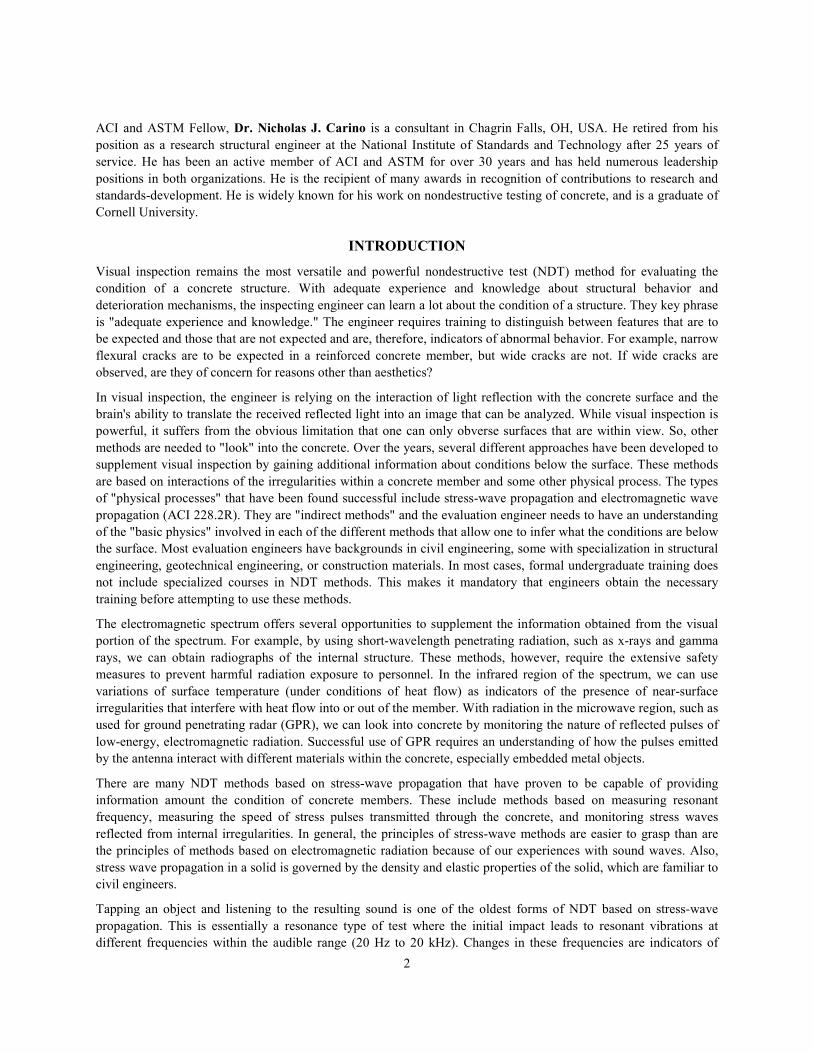
frequency is associated with a specific vibrational mode shape. When a concrete plate is struck, it also "rings" at a
resonant frequency and has an associated vibrational mode shape. There are two general mode shapes that can occur
in an elastic plate as shown in Fig. 5. The mode shape in Fig. 5(a) is symmetrical with respect to the mid-plane of
the plate. This is associated with the thickness mode frequency. The other mode shape is anti-symmetrical because
opposite faces move in the same direction and is associated with lower frequency flexural vibrations.
Figure 5—Thickness and flexural modes of vibration of free plate
The thickness mode of vibration for a free plate in impact-echo testing has been related to what is known as "a plate
Lamb wave" (Gibson and Popovics 2005). The theory of Lamb waves is complex and no attempt is made to discuss
it here. The interested reader will find the topic covered in textbooks on elastic wave propagation, such as
Achenbach (1973) and Graff (1975). What is important about the symmetrical Lamb wave is that the wave speed is
less than that for the propagation of a P-wave in a semi-infinite half space as given in Table 1. For thin plates, the
plate wave speed is given by the following approximate relationship (Graff 1975):
2(1 )
plate
EC
vρ≈
− (2)
If we make the ratio of the speed given by Eq.(2) to the P-wave speed from Table 1, we obtain the following
relationship:
2
(1 )(1 2 )
(1 )(1 )
plate
p
C
C
ν νν ν
+ −≈
− − (3)
Thus the plate wave speed is related to the P-wave speed according to the value of Poisson's ratio. Table 3 shows the
ratio given by Eq. (3) for a range of values of Poisson's ratio that is typical for concrete.
Table 3—Ratio of plate wave speed to P-wave speed
Poisson's ratio
Cplate/Cp
Eq. (3) Gibson and Popovics (2005)
0.18
0.20
0.22
0.976
0.968
0.959
0.955
0.953
0.950

9
Gibson and Popovics (2005) solved the governing equations for the symmetric thickness mode vibration of plate and
determined the wave-speed ratios shown in the last column of Table 3. While the numbers in columns 2 and 3 are
not exactly the same, they show that the plate wave speed is slightly lower than the P-wave speed. Based on
empirical observations, Sansalone (1997) suggested that the ratio is 0.96, and this value was used in the
development of ASTM C1383.
In summary, impact-echo testing is based on exciting the thickness mode of vibration of a plate. The thickness
frequency (fT) is related to the plate wave speed (Cplate) and plate thickness by the following equation:
2
plate
T
CT
f= (4)
Thus the objective in impact-echo testing is to determine the thickness frequency and this can be used to calculate
the depth of the reflecting interface. The value of the thickness frequency is obtained from the time domain
waveform by signal processing as is explained in a subsequent section.
Prismatic shapes
The above discussion applies to a "plate-like" element, which is defined as a plate with lateral dimension at least six
times the plate thickness (ASTM C1383). These minimum lateral dimensions are required so that the impact
response is dominated by the thickness mode resonance. When we have a prismatic member, such as a beam or a
column, the side boundaries also reflect stress waves and the picture of reflected wavefronts with the passage of time
is more complicated than shown in Fig. 4. The multiple reflections from the boundaries of the member result in
many vibrational modes, collectively termed "cross-sectional modes" (Sansalone and Street 1997). As a result, when
a solid column or beam is subjected to an impact, the response comprises several characteristic frequencies.
Figure 6 shows the cross-sectional modes of vibration that will be excited when the side of a square column is
subjected to a point impact (Lin and Sansalone 1992a, 1992b). The first mode is analogous to the thickness mode of
a plate, but because of flexibility in two directions, the apparent wave speed is less than the plate wave speed. The
amplitude spectrum in Fig. 6 shows the response of the solid square column. The six mode shapes are associated
with peaks in the amplitude spectrum. Each frequency is a multiple of the Mode 1 frequency, as shown by the
tabulated values. Popovics (1997) has shown that the frequency ratios for the different modes are a function of
Poisson's ratio, and the values in Fig. 6 are applicable to a Poisson's ratio of 0.2, which is a typical value for
concrete. This dependence on Poisson's ratio is expected because the modes are set up by the interaction of the P-
wave and S-wave, and the ratio of wave speeds is a function of Poisson's ratio (see Table 1).
The cross-sectional modes of prismatic members with round or rectangular cross-sections will have different
frequency ratios than shown in Fig. 6 (Lin and Sansalone 1992a; Sansalone and Streett 1997). While the amplitude
spectrum for a sound prismatic member is complex due to multiple resonances, the presence of an internal
discontinuity will disrupt the pattern of frequency peaks. This allows one to determine whether the member is solid
or contains internal irregularities. Thus an important step when testing prismatic members is to calculate the
expected ratios of frequency values for a solid member (Sansalone and Street 1997). If the impact-echo test results
confirm the calculated frequency ratios, it can be assumed that the member is solid at that test location. If the pattern
of peaks is different than expected, it can be assumed that there is some type of irregularity and additional
investigation using different test locations and impact durations may be able to determine the depth of the
irregularity.

10
Figure 6—Mode shapes and frequency ratios for a solid prismatic member with a square cross section (Lin
and Sansalone 1992)
Frequency analysis
The key feature of the impact-echo method, which makes it possible to determine the thickness of a plate or the
depth of an internal reflecting interface, is the extraction from the time domain waveform the frequency
corresponding to the plate thickness mode of vibration. This is accomplished by using the principle of Fourier
series, which states that any periodic function f(t) can be represented as the sum of a constant term plus a series of
sine curves with different amplitudes and phase angles.2 In mathematical terms, the principle can be written as
follows:
( )0
1
0
( ) sin 2
1
n
n o nf t a a n f t
fT
π φ= + +
=
∑ (5)
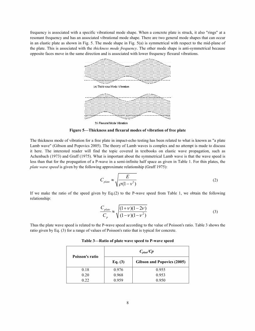
In Eq. (5), T is the period of the waveform, that is, the waveform repeats after a time interval equal to T. Thus, for
example, the periodic waveform in Fig. 7(a) can be created by the sum of a constant and four sine curves with
different phase angles as shown in Fig. 7(b). The sine curves have different phase angles because the peaks and
valleys do not occur at the same time.
2 To gain a better understanding of Fourier series, the reader may wish to visit the Web site http://www.fourier-
series.com/fourierseries2/fourier_series_tutorial.html, which includes a series of lectures and applets on different
aspects of this subject
11
-1.5
-1.0
-0.5
0.0
0.5
1.0
1.5
2.0
0 50 100 150 200
Amplitude
Time
Period
T
(a)
-1.5
-1.0
-0.5
0.0
0.5
1.0
1.5
2.0
0 50 100 150 200
Constant
fo
2fo
3fo
4fo
sum
Amplitude
Time
(b)
Figure 7—A repeating waveform (a) with a period T is equivalent to the sum of a constant and a series of sine
curves with different amplitudes and phase angles as shown in (b).
In the impact-echo method, the time-domain waveform is obtained by sampling the output of the receiver at small
time steps. Thus the waveform is composed of a series of discrete points rather than a continuous function as shown
in Fig. 7(a). The discrete Fourier transform (DFT) is the technique used to obtain the frequency components in a
sampled waveform. If there are N points in the sampled waveform, the output of the DFT will be a series of N/2
complex numbers. Each complex number can be converted to an amplitude and phase angle using the principles for
manipulating complex numbers. The resulting amplitude spectrum shows the amplitudes of the various frequency
components (sine curves) that comprise the waveform. In impact-echo testing, the phase spectrum is not used. In the
spectral analysis of surface waves (SASW) method, the phase spectrum is used exclusively.
The fast Fourier transform (FFT) is an efficient algorithm for performing the DFT calculations. The program is
designed to work with time-domain records with the number of points equal to a power of 2. Thus typical numbers
of points in the waveform are 512, 1024, 2048, or 4096. The amplitude spectrum will contain N/2 points.
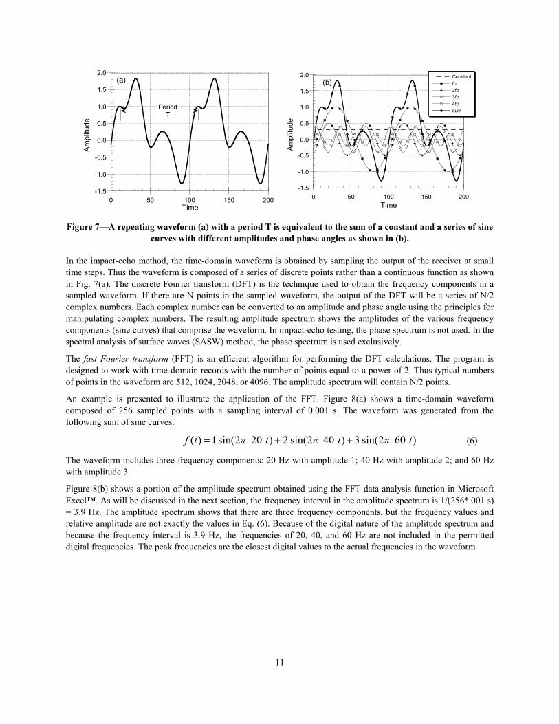
An example is presented to illustrate the application of the FFT. Figure 8(a) shows a time-domain waveform
composed of 256 sampled points with a sampling interval of 0.001 s. The waveform was generated from the
following sum of sine curves:
( ) 1sin(2 20 ) 2 sin(2 40 ) 3 sin(2 60 )f t t t tπ π π= + +� � � � � � (6)
The waveform includes three frequency components: 20 Hz with amplitude 1; 40 Hz with amplitude 2; and 60 Hz
with amplitude 3.
Figure 8(b) shows a portion of the amplitude spectrum obtained using the FFT data analysis function in Microsoft
Excel™. As will be discussed in the next section, the frequency interval in the amplitude spectrum is 1/(256*.001 s)
= 3.9 Hz. The amplitude spectrum shows that there are three frequency components, but the frequency values and
relative amplitude are not exactly the values in Eq. (6). Because of the digital nature of the amplitude spectrum and
because the frequency interval is 3.9 Hz, the frequencies of 20, 40, and 60 Hz are not included in the permitted
digital frequencies. The peak frequencies are the closest digital values to the actual frequencies in the waveform.

12
-6.0
-4.0
-2.0
0.0
2.0
4.0
6.0
0 0.05 0.1 0.15 0.2 0.25
Amplitude
Time, s
(a)
0.0
0.2
0.4
0.6
0.8
1.0
1.2
0 50 100 150
Amplitude
Frequency, Hz
(b)
19.5 Hz
39.1 Hz58.6 Hz
∆f = 3.9 Hz
Figure 8—(a) A digitized time-domain waveform composed of three frequency components; (b) the amplitude
spectrum obtained from the FFT
In the impact-echo test, the time-domain waveform represents the surface motion associated with different resonant
modes that may be present. Transformation of the waveform into the frequency domain by using the FFT reveals the
predominant frequency components in the response. These frequency components will appear as peaks in the
amplitude spectrum. Figure 9(a) shows an example of a time-domain waveform obtained from an impact-echo of a
solid concrete plate. The sampling interval was 2 µs and there were 1024 points in the total record. The initial large
negative voltage is due to the arrival of the surface wave, and the subsequent oscillations are from the thickness
mode resonance of the plate. Figure 9(b) shows a portion of the corresponding amplitude spectrum up to 40 kHz.
The dominant peak at 7.81 kHz is the thickness mode frequency of the plate. If the plate wave speed were known,
Eq. (4) can be used to convert the frequency to a thickness. For example, if the value of Cplate = 3900 m/s, the
thickness would be 3900/(2*7810) = 0.25 m.
-0.4
-0.3
-0.2
-0.1
0.0
0.1
0.2
0.3
0.4
0 500 1000 1500 2000
Volts
Time, µs
(a)
0.0
0.2
0.4
0.6
0.8
1.0
1.2
0 5 10 15 20 25 30 35 40
Amplitude
Frequency, kHz
7.81 kHz(b)
Figure 9—(a) Time-domain waveform from impact-echo test of solid concrete plate; (b) amplitude spectrum
showing peak associated with the thickness mode frequency (Impact-Echo Instruments LLC).
In summary, one of the breakthroughs that lead to the development of the impact-echo method is the use of the
frequency domain to analyze test results. The FFT algorithm allows rapid conversion of the time domain waveform
to the amplitude spectrum. The amplitude spectrum reveals the predominant frequency components that are
associated with thickness mode resonances. The next section discusses how we can control the frequency resolution
in the amplitude spectrum.

13
Data acquisition parameters
Users of the impact-echo method need to understand the relationships among the data acquisition parameters used to
acquire time domain waveforms. The key parameters include:
• Sampling interval;
• Record length;
• Voltage range; and
• Trigger level.
The sampling interval is the time between each sampled point in the time-domain waveform. The inverse of the
sampling interval is the sampling frequency. When the waveform is transformed into the frequency domain, the
maximum frequency in the amplitude spectrum is one-half of the sampling frequency. The record length is the
number of points in the time-domain waveform multiplied by the sampling interval. These parameters are important
because they affect the amplitude spectrum. Table 4 summarizes the relationships among sampling rate, number of
points in the waveform, and frequency resolution (or frequency interval) in the amplitude spectrum. Basically, the
frequency resolution is the inverse of the record length. The last two columns show the values of the parameters for
two examples. The first example is commonly used for routine impact-echo testing. In the second example, the
sampling frequency is reduced by one-half and the number of points is doubled. This makes the record length four
times longer and the frequency interval is one-fourth of the value in the first example.
Table 4—Data acquisition parameters
Parameters Examples
Symbol Description Example 1 Example 2
∆t Sampling interval; time between successive points in waveform. 2 µs 4 µs
fs Sampling frequency; inverse of ∆t. 500 kHz 250 kHz
fmax Maximum frequency in amplitude spectrum; one-half of fs. 250 kHz 125 kHz
N Number of points in waveform (record). 1024 2048
N ∆t Record length; duration of waveform. 2.048 ms 8.192 ms
∆f Frequency resolution in amplitude spectrum; equal to inverse of
record length.
0.488 kHz 0.122 kHz
Ideally, the frequency resolution ∆f should be small to increase the accuracy of the calculated depths using Eq. (4).
As shown in Table 4, this can be achieved by increasing the record length, either by reducing the sampling
frequency, or increasing the number of sampled points, or both. If, however, the record length is made too long,
stress waves reflected from the side boundaries will complicate the waveform and the resulting amplitude spectrum
(Sansalone and Streett 1997).
Because of the digital nature of the data in impact-echo testing, there are constraints on the accuracy of the
calculated plate thickness or depth of an irregularity based on using Eq. (4). When a peak is observed in the
amplitude spectrum at a frequency f, the actual frequency can be within the range of f ± ∆f/2. The range of the actual
thickness or depth that would result in the same peak frequency in the digital spectrum is as follows:
2 1
2 22 2
plate plateC CT T
f ff f
− = −∆ ∆ − +
(6)
Table 5 shows the range of depths calculated by Eq. (6) for different peak frequencies in an amplitude spectrum for
a plate wave speed of 4000 m/s and different frequency intervals. Because of the inverse relationship between depth
and frequency, the inherent uncertainty in the actual depth based on an impact-echo test increases with depth.

14
Table 5—Range of actual depth for Cplate = 4000 m/s and different frequency intervals
Frequency,
kHz
Calculated
Depth, mm
Depth Range, mm
∆f = 0.488 kHz ∆f = 0.244 kHz ∆f = 0.122 kHz
3.33 600 559 to 647 579 to 623 589 to 611
4.00 500 471 to 532 485 to 516 492 to 508
5.00 400 381 to 421 390 to 410 395 to 405
6.67 300 289 to 311 295 to 306 297 to 303
10.00 200 195 to 205 198 to 202 199 to 201
20.00 100 99 to 101 99 to 101 100 to 100
The other data acquisition parameters are the voltage level and trigger level. The voltage level should match the
highest voltage that will be generated by the receiver. The voltage output depends on many factors such as the
distance between receiver and impact point, the smoothness of the test surface, the distance to the reflecting
interface, the type of element being tested, and the contact time. The voltage level should be set low enough so that
the recorded waveform is easily observed when displayed on the computer screen. This allows the user an
opportunity to check whether the waveform is valid. Invalid waveforms are usually due to improper coupling to the
surface or false triggers. See Sansalone and Street (1997) for examples of invalid waveforms. If the voltage level is
set too low, the waveform is cut-off or "clipped." In some cases, it is beneficial to clip the R-wave portion of the
waveform (Sansalone and Carino 1986; Carino et al. 1986). This will be shown in the next section. If the voltage
level is set too high, it will not have a significant effect on the amplitude spectrum.
The trigger level is used to instruct the data acquisition system when to start storing data. When the signal from the
receiver matches the trigger condition, the specified number of data points is stored in memory. Typically, a certain
duration of signal before the trigger condition is also stored. This "pre-trigger" information is useful in assessing the
validity of the signal. In cases where there is high electrical noise or ambient vibrations, a higher trigger level may
be needed to avoid false triggering.
Frequency content of impact force
One of the most important steps in impact-echo testing is the selection of the contact time (tc)of the impact. This
section reviews the main concepts that should be understood by the user. From the earliest research on impact-echo
testing (Sansalone and Carino 1986), it was determined that a steel ball is a convenient impactor. In the early work,
the ball was dropped onto the horizontal surface, in subsequent work the ball was attached to a small high-strength
steel rod to produce a small hammer or the rod was attached to base so that a "plucking" action could be used to
generate the impact.
We begin with the shape of the force time curve produced by the impact of a steel ball. It has been assumed that the
force-time curve can be approximated by a half-cycle sine curve with the following equation
( ) sin
0
max
c
c
tF t F
t
F for t t
π =
= >
(7)
Figure 10 shows two examples of force-time curves for impacts of different durations (the units of the time axis are
not important for this discussion). The principle of Fourier series can be applied to these curves, that is, the force-
time functions can be represented as the sum of a constant term plus a series of sine curves of different amplitudes
and phase angles. This is illustrated in Figure 11.

15
-0.2
0.0
0.2
0.4
0.6
0.8
1.0
1.2
0 1 2 3 4 5 6
Amplitude
Time
(a)
-0.2
0.0
0.2
0.4
0.6
0.8
1.0
1.2
0 1 2 3 4 5 6
Amplitude
Time
(b)
Figure 10—Examples of force-time functions with different contact times
Figure 11(a) shows that by taking the sum of a constant and four sine curves with the frequencies, amplitudes, and
phase shifts shown we obtain a close approximation of the shape of the force-time curve in Fig. 10(a). Likewise, by
taking the sum of the constant term and sine curves shown in Fig. 11(b), we obtain a good approximation of the
shape of the force-time curve in Fig. 10(b). Thus we can view effect of impact with a ball to be the same as applying
a series of sine function inputs at the impact point.
-0.4
0.0
0.4
0.8
1.2
0 1 2 3 4 5 6
Constant
cos t
cos 2t
cos 4t
cos 6t
Sum
Amplitude
Time
(a)
-0.4
-0.2
0.0
0.2
0.4
0.6
0.8
1.0
1.2
0 1 2 3 4 5 6
Constant
cos t
cos 2t
cos 3t
cos 4t
cos 5t
Sum
Amplitude
Time
(b)
Figure 11—Illustration of how to the sum sine curves of different amplitudes, frequencies, and phases can
produce a function similar to the force-time function assumed in impact-echo testing
The Fourier transform of a half-cycle sine function has a closed form solution (Bracewell 1978). The shape of the
amplitude spectrum is of this ideal force-time function is shown in Fig. 12. The axes have been normalized by the
contact time so that this amplitude spectrum is applicable to any duration of contact time. We see that the spectrum
has zeros are frequencies of 1.5/tc, 2.5/tc, 3.5/tc, and so forth. This spectrum represents the frequency content of the
impact force. As a simplification, we can say that the maximum useable frequency is a normalized frequency value
of 1. This means that if the contact time is 40 µs, the maximum useable frequency is 1/(40 ×10-6) = 25 kHz. The key
point is as follows: In order to excite the thickness mode frequency in an impact-echo test, the maximum useable
frequency contained in the impact must be greater than the thickness frequency. For example, assume that the plate
wave speed is 4000 m/s and we would like to determine whether there is a void at a depth of 75 mm in a concrete
wall. From Eq. (4), the thickness mode frequency would be 4000/(2 ×0.075) = 27 kHz. The inverse of this frequency
is the maximum contact time that can be used, which would be approximately 40 µs.

16
0.0
0.1
0.2
0.3
0.4
0.5
0.6
0.7
0 1 2 3 4 5
Amplitude/Contact Time
Frequency X Contact Time
Useable upper frequency
Figure 12—Normalized amplitude spectrum for a force-time function having the shape of a half-cycle sine
curve
To assist in understanding the relationship between contact time and resonant frequency, let us consider ASTM Test
Method C215. This is a laboratory test method for measuring the resonant frequency of specimens for different
modes of vibration. In the classical method, the specimen is forced to vibrate by a driver that applies a continuous
sinusoidal vibration to the specimen. The motion of the specimen is measured by a transducer. To determine the
resonant frequency of the specimen, the driver frequency is increased slowly until there is maximum response as
indicated by maximum amplitude of the transducer signal. The alternative method is to strike the specimen with a
small impactor and determine the frequency content in the response by determining the amplitude spectrum. The
impact is, in effect, the same as applying many sinusoidal frequencies at one time. If the impact contains a frequency
component equal to the resonant frequency of the specimen, the specimen will respond to that component and
vibrate at its resonant frequency. If the contact time is too long, there will no high frequency components and the
specimen will not vibrate at its resonant frequency. As an analogy, consider a small bell that is struck by soft rubber
hammer and by a small metal hammer. Because the contact time with the rubber hammer is too long, the impact
would not contain the high frequency component corresponding to the pitch of the bell, and the bell would not ring.
The metal hammer, on the other hand, would produce a short duration impact containing the required frequency
component, and the bell would ring. The same principles apply when performing an impact-echo test on a concrete
element; the impact has to contain enough energy at the thickness mode frequency in order to excite that mode of
vibration.
For the elastic impact of a steel ball dropped onto a concrete surface from a given height, the duration of an elastic
impact can be calculated from the diameter of the ball and the densities and elastic properties of steel and concrete.
(Goldsmith 1965). The solution shows that the contact time is not sensitive to the drop height (or the speed of the
ball at the time of impact). For typical values of Young's modulus of elasticity and Poisson's ratio of concrete, the
contact time in microseconds is approximately 4.3 times the ball diameter in mm (Sansalone and Carino 1986). Thus
a 10 mm ball will produce an impact with a contact time of about 43 µs. In practice, the actual contact time can be
expected to be longer than this theoretical value due to inelastic behavior in the concrete.

17
Table 6 shows the approximate contact times produced by steel balls of different diameters striking a smooth
concrete surface. If we assume that the maximum useable frequency in the amplitude spectrum of the force-time
curve is the inverse of the contact time, the third column shows the corresponding maximum useable frequencies.
The fourth column shows the minimum depths that can be measured for a plate wave speed of 4000 m/s.
Table 6—Approximate relationships between ball diameter and minimum measurable depth for
Cplate = 4000 m/s
Ball Diameter,
mm
Approximate
Contact Time, µs
Maximum Useable
Frequency, kHz
Minimum Measurable
Depth, mm
5 22 47 43
6 26 39 52
7 30 33 60
8 34 29 69
9 39 26 77
10 43 23 86
12 52 19 103
15 65 16 129
20 86 12 172
The duration of the impact in an impact-echo test can be estimated from the width of the of R-wave portion of the
waveform (Sansalone and Carino 1986). Figure 13(a) shows the initial portion of the waveform in Fig 9(a) at an
expanded scale. The approximate width of the R-wave signal is 50 µs, and we would expect a maximum useable
frequency of about 20 kHz. Figure 13(a) shows the amplitude spectrum for the 50-µs duration portion of the
waveform. We see that the spectrum has the expected shape shown in Fig. 12, and it is confirmed that the maximum
useable frequency in the impact is about 20 kHz.
-0.4
-0.3
-0.2
-0.1
0.0
0.1
0.2
160 180 200 220 240 260
Volts
Time, µs
(a)
50 µs
0.0
1.0
2.0
3.0
4.0
5.0
0 10 20 30 40 50
Amplitude
Frequency, kHz
(b)
Figure 13—a) Initial portion of waveform shown in Fig. 9(a) and the estimate of the duration of the R-wave;
(b) the amplitude spectrum of the 50 µs portion of the waveform.
When short contact times are used, the relative amplitude of the R-wave signal is large compared with the signal
associated with thickness mode resonance. For example, consider the waveform shown in Fig. 14(a), which was
obtained with a contact time of about 20 µs. It is seen that the surface wave signal is about four times the amplitude
of the signal associated with thickness resonance. The corresponding amplitude spectrum is shown in Fig. 14(b).
There are two sharp peaks. The peak at about 12 kHz corresponds to the thickness mode frequency. The peak at
about 1 kHz is associated with resonance of the transducer and can be ignored. The amplitude spectrum has
additional peaks beyond 20 kHz. It is not certain whether these peaks are significant or whether they are realted to
the superposition of the spectrum associated with the R-wave.

18
There are two approaches for reducing or removing the effect of the spectrum associated with the R-wave, which
will have a shape similar to Fig. 9(b). One approach is to reduce the voltage level on the data acquisition system so
that the R-wave portion of the signal is clipped. Figure 15(a) shows the same waveform as in Fig. 14(a) except that
the voltage level has been set to ±0.15 V. The resulting amplitude spectrum is significantly different than the one in
Fig. 14(b). The frequency "hump" between 15 kHz and 50 kHz that is present in Fig. 14(b) has been reduced. We
can conclude that the peaks beyond 15 kHz are not likely related to a smaller and shallower reflector, and may be
due to higher modes of the thickness frequency.
-0.8
-0.6
-0.4
-0.2
0.0
0.2
0.4
0 500 1000 1500 2000
Volts
Time, µs
(a)
0.0
0.2
0.4
0.6
0.8
1.0
1.2
0 10 20 30 40 50 60Amplitude
Frequency, kHz
(b)
Figure 14—Waveform and spectrum for an impact-echo test with a short contact time (Impact-Echo
Instruments LLC).
-0.20
-0.15
-0.10
-0.05
0.00
0.05
0.10
0.15
0.20
0 500 1000 1500 2000
Volts
Time, µs
(a)
0.0
0.2
0.4
0.6
0.8
1.0
1.2
0 10 20 30 40 50 60
Amplitude
Frequency, kHz
(b)
Figure 15—(a) The same waveform as in Fig. 14(a), but the signal has been clipped at ±0.15 V; (b) the
amplitude spectrum for the clipped waveform.
The other approach is to remove completely the portion of the waveform associated with the R-wave. This has been
done in Fig. 16(a). The voltage value was set to zero so as to remove the first large negative peak and the first large
positive peak shown in Fig. 14(a). The resulting amplitude spectrum shown in Fig. 16(b) is similar to the spectrum
for the clipped waveform.
In this example, both approaches were equally effective in simplifying an amplitude spectrum that contained a
significant component due to the spectrum associated with the high amplitude R-wave signal. This is not always the
case, and removal of the R-wave will, in general, result in less complex spectra than clipping the signal. The
clipping approach can be implemented while data are being acquired by simply reducing the voltage level for the
data acquisition system and repeating the test. The removal of the R-wave, however, has to be done as a post-
processing step after the data have been acquired and stored.
19
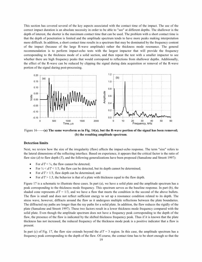
This section has covered several of the key aspects associated with the contact time of the impact. The use of the
correct impact duration is an absolute necessity in order to be able to "see" at different depths. The shallower is the
depth of interest, the shorter is the maximum contact time that can be used. The problem with a short contact time is
that the depth of penetration is limited and the amplitude spectrum tends to have more peaks making interpretation
more difficult. In addition, a short contact time results in a spectrum that may be dominated by the frequency content
of the impact (because of the large R-wave amplitude) rather the thickness mode resonance. The general
recommendation is to perform impact-echo tests with the largest impactor that will provide the frequency
corresponding to the thickness mode of a solid section, and then repeat the test with a smaller impactor to see
whether there are high frequency peaks that would correspond to reflections from shallower depths. Additionally,
the effect of the R-wave can be reduced by clipping the signal during data acquisition or removal of the R-wave
portion of the signal during post-processing.
-0.15
-0.10
-0.05
0.00
0.05
0.10
0.15
0.20
0 500 1000 1500 2000
Volts
Time, µs
(a)
0.0
0.2
0.4
0.6
0.8
1.0
1.2
0 10 20 30 40 50 60
Amplitude
Frequency, kHz
(b)
Figure 16——(a) The same waveform as in Fig. 14(a), but the R-wave portion of the signal has been removed;
(b) the resulting amplitude spectrum.
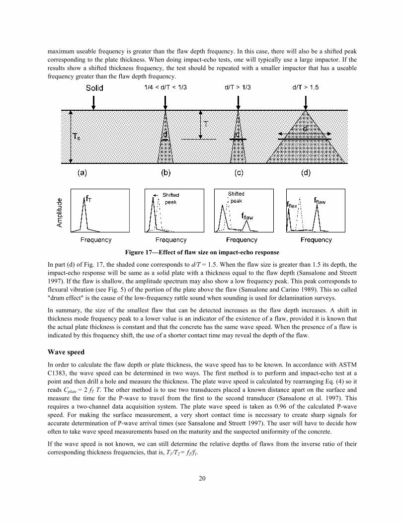
Detection limits
Next, we review how the size of the irregularity (flaw) affects the impact-echo response. The term "size" refers to
the lateral dimensions of the reflecting interface. Based on experience, it appears that the critical factor is the ratio of
flaw size (d) to flaw depth (T), and the following generalizations have been proposed (Sansalone and Streett 1997):
• For d/T < ¼, the flaw cannot be detected;
• For ¼ < d/T < 1/3, the flaw can be detected, but its depth cannot be determined;
• For d/T > 1/3, flaw depth can be determined; and
• For d/T > 1.5, the behavior is that of a plate with thickness equal to the flaw depth.
Figure 17 is a schematic to illustrate these cases. In part (a), we have a solid plate and the amplitude spectrum has a
peak corresponding to the thickness mode frequency. This spectrum serves as the baseline response. In part (b), the
shaded cone represents d/T = 1/3, and we have a flaw that meets the condition in the second of the above bullets.
The flaw is small and does not reflect sufficient energy to set up a resonance condition related to its depth. The
stress wave, however, diffracts around the flaw as it undergoes multiple reflections between the plate boundaries.
The diffracted ray paths are longer than the ray paths for a solid plate. In addition, the flaw reduces the rigidly of the
plate (Sansalone and Streett 1997). These two factors result in a lower thickness mode frequency compared with the
solid plate. Even though the amplitude spectrum does not have a frequency peak corresponding to the depth of the
flaw, the presence of the flaw is indicated by the shifted thickness frequency peak. Thus if it is known that the plate
thickness has not increased, the reduced frequency of the thickness mode peak is a positive indicator that a flaw is
present.
In part (c) of Fig. 17, the flaw size extends beyond the d/T = 3 region. In this case, the amplitude spectrum has a
frequency peak corresponding to the depth of the flaw. Of course, the contact time has to be short enough so that the
20
maximum useable frequency is greater than the flaw depth frequency. In this case, there will also be a shifted peak
corresponding to the plate thickness. When doing impact-echo tests, one will typically use a large impactor. If the
results show a shifted thickness frequency, the test should be repeated with a smaller impactor that has a useable
frequency greater than the flaw depth frequency.
Figure 17—Effect of flaw size on impact-echo response
In part (d) of Fig. 17, the shaded cone corresponds to d/T = 1.5. When the flaw size is greater than 1.5 its depth, the
impact-echo response will be same as a solid plate with a thickness equal to the flaw depth (Sansalone and Streett
1997). If the flaw is shallow, the amplitude spectrum may also show a low frequency peak. This peak corresponds to
flexural vibration (see Fig. 5) of the portion of the plate above the flaw (Sansalone and Carino 1989). This so called
"drum effect" is the cause of the low-frequency rattle sound when sounding is used for delamination surveys.
In summary, the size of the smallest flaw that can be detected increases as the flaw depth increases. A shift in
thickness mode frequency peak to a lower value is an indicator of the existence of a flaw, provided it is known that
the actual plate thickness is constant and that the concrete has the same wave speed. When the presence of a flaw is
indicated by this frequency shift, the use of a shorter contact time may reveal the depth of the flaw.
Wave speed
In order to calculate the flaw depth or plate thickness, the wave speed has to be known. In accordance with ASTM
C1383, the wave speed can be determined in two ways. The first method is to perform and impact-echo test at a
point and then drill a hole and measure the thickness. The plate wave speed is calculated by rearranging Eq. (4) so it
reads Cplate = 2 fT T. The other method is to use two transducers placed a known distance apart on the surface and
measure the time for the P-wave to travel from the first to the second transducer (Sansalone et al. 1997). This
requires a two-channel data acquisition system. The plate wave speed is taken as 0.96 of the calculated P-wave
speed. For making the surface measurement, a very short contact time is necessary to create sharp signals for
accurate determination of P-wave arrival times (see Sansalone and Streett 1997). The user will have to decide how
often to take wave speed measurements based on the maturity and the suspected uniformity of the concrete.
If the wave speed is not known, we can still determine the relative depths of flaws from the inverse ratio of their
corresponding thickness frequencies, that is, T1/T2 = f2/f1.

21
Planning and verification
Sansalone and Streett (1997) and ACI 228.2R provide helpful information to assist in planning an impact-echo test
program. As much information about the structure should be gathered before testing. The expected frequencies for
different possible conditions should be calculated for assumed values of wave speed. This is especially important
when testing beams and columns, which will have multiple peaks in the amplitude spectra. Based on expected
frequencies, the size of the impactor should be selected to ensure that the impact will deliver the necessary
frequency components. The record length should be selected to maximize frequency resolution and at the same time
avoid recording the arrival of reflected waves from side boundaries. It is recommended that interpretation of results
be done in the field rather than recording data and then trying to sort through the interpretation at the office
(Sansalone and Streett 1997).
For large and complex projects it may worthwhile to perform finite element simulations of impact-echo tests to gain
a better understanding of the expected responses for different assumed conditions. Such analyses should be done by
engineers with experience in using computer programs that can model stress wave propagation.
After data interpretation has been completed, selective verification of key conclusions should be undertaken by
drilling cores or drilling holes in combination with visual inspection using a borescope. Verification is especially
important when evaluating a complex structure. Locations for invasive inspection should include points that are
deemed to be without flaws as well as points were flaws are indicated. Verification serves to instill confidence in the
evaluation engineer as well as the client.
SUMMARY
Successful use of advanced NDT methods requires a good understanding of the underlying principles that permit the
detection of irregularities within concrete members. Failure to acquire the necessary background knowledge exposes
the engineer to making incorrect interpretations from test results. Such errors can harm the engineer's reputation, and
more importantly it can cast doubt on the reliability of a method that have been developed on the basis of careful
research. The engineer needs to understand the capabilities and limitations of a test method to avoid raising
expectations beyond the known limits of the method. Thus it is recommended that when an advanced NDT system is
to be added to the toolbox of evaluation tools, the engineer should factor in the cost of training as part of the initial
cost to acquire the test system. The investment will pay off in a short time if the engineer is able to deliver accurate
evaluations. The engineer's reputation will be enhanced and potential new clients will have confidence in hiring that
engineer.
A review of the key aspects of the impact-echo method has been presented to illustrate the extent of knowledge that
is needed to use an advanced NDT method. The scope of the topics covered in this review is applicable to other
methods besides the impact-echo method. The closing thought is that the engineer should avoid the temptation to
buy new hardware, install the software, and proceed with field testing without additional training. The reality is that
most advanced NDT methods are based on complex principles and this complexity needs to be appreciated rather
than ignored.

22
REFERENCES
Achenbach, J.D., 1973, Wave Propagation in Elastic Solids, North Holland Publishing Co.
ACI 228.2R, "Nondestructive Test Methods for Evaluation of Concrete in Structures," American Concrete Institute,
Farmington Hills, MI.
ASTM C215, "Test Method for Fundamental Transverse, Longitudinal, and Torsional Resonant Frequencies of
Concrete Specimens, Annual Book of ASTM Standards Vol. 04.02, ASTM, West Conshohocken, PA.
ASTM C1383, "Test Method for Measuring the P-Wave Speed and the Thickness of Concrete Plates using the
Impact-Echo Method," Annual Book of ASTM Standards Vol. 04.02, ASTM, West Conshohocken, PA.
ASTM D 4580, "Standard Practice for Measuring Delaminations in Concrete Bridge decks by Sounding," Annual
Book of ASTM Standards Vol. 04.03, ASTM, West Conshohocken, PA.
Bracewell, R., 1978, The Fourier Transform and its Applications, 2nd Ed., McGraw-Hill Book Co., 444 p.
Carino, N.J., 2004, "Stress Wave Propagation Methods," In Handbook on Nondestructive Testing of Concrete 2nd
Edition, V.M. Malhotra and N.J. Carino, eds.. CRC Press, Boca Raton, FL and ASTM International, West
Conshohocken, PA.
Carino, N.J., Sansalone, M., and Hsu, N.N., 1986, "Flaw Detection in Concrete by Frequency Spectrum Analysis of
Impact-Echo Waveforms," in International Advances in Nondestructive Testing, Ed. W.J. McGonnagle,
Gordon & Breach Science Publishers, New York, pp. 117-146
Cheng, C., and Sansalone, M., 1993b, "Effects on Impact-Echo Signals Caused by Steel Reinforcing Bars and Voids
Around Bars," ACI Materials Journal, Vol. 90, No. 5, Sept-Oct., pp. 421-434.
Gibson, A. and Popovics, J.A., 2005, "Lamb Wave Basis for Impact-Echo Method Analysis," J. of Engineering
Mechanics (ASCE), Vol. 131, No. 4, April, pp. 438-443.
Goldsmith, W., 1965, Impact: The Theory and Physical Behavior of Colliding Solids, Edward Arnold Press,
Ltd., pp. 24-50.
Graff, K. F., Wave Motion in Elastic Solids, Ohio State University Press, 1975.
Krautkrämer, J. and Krautkrämer, H., 1990, Ultrasonic Testing of Materials, 4th Ed., Springer-Verlag, New York.
Lin, Y. and Sansalone, M., 1992a, "Detecting Flaws in Concrete Beams and Columns Using the Impact-Echo
Method," ACI Materials Journal, Vol. 89, No. 4, July-August 1992, pp. 394-405.
Lin, Y., and Sansalone, M., 1992b, "Transient Response of Thick Circular and Square Bars Subjected to Transverse
Elastic Impact," Journal of the Acoustical Society of America, Vol. 91. No.2, February 1992, pp. 885-893.
Popovics, J.A., 1997, "Effect of Poisson's Ratio on Impact-Echo Method Analysis," J. of Engineering Mechanics
(ASCE), Vol. 123, No. 8, August 1997, pp. 843-851.
Sansalone, M, 1997, "Impact-Echo: The Complete Story," ACI Structural Journal, Vo. 94, No. 6, November-
December, pp. 777-786.
Sansalone, M., and Carino, N.J., 1986, "Impact-Echo: A Method for Flaw Detection in Concrete Using Transient
Stress Waves," NBSIR 86-3452, National Bureau of Standards, Sept., 222 p. (Available from NTIS,
Springfield, VA, 22161, PB #87-104444/AS)
Sansalone, M. and Carino, N.J., 1989, "Detecting Delaminations in Concrete Slabs with and without Overlays Using
the Impact-Echo Method," Journal of the American Concrete Institute, Vol. 86, No. 2, March, pp. 175-184.
Sansalone, M., and Carino, N. J., 1990, "Finite Element Studies of the Impact-Echo Response of Layered Plates
Containing Flaws," in International Advances in Nondestructive Testing, 15th Ed. W. McGonnagle,
Gordon & Breach Science Publishers, New York, 1990, pp. 313-336.
Sansalone, M., and Streett, W. B., 1997, Impact-Echo: Nondestructive Testing of Concrete and Masonry,
Bullbrier Press, Jersey Shore, PA.
Sansalone, M., Lin, J.M., and Streett, W.B., 1997a,"A Procedure for Determining P-Wave Speed in Concrete for
Use in Impact-Echo Testing Using a P-Wave Speed Measurement Technique," ACI Materials Journal, Vol.
94, No. 6, November-December 1997, pp. 531-539.