TRAINING CONFIDENCE CALIBRATED CLASSIFIERS FOR …

Published as a conference paper at ICLR 2018

TRAINING CONFIDENCE-CALIBRATED CLASSIFIERSFOR DETECTING OUT-OF-DISTRIBUTION SAMPLES

Kimin Lee∗ Honglak Lee§ ,† Kibok Lee† Jinwoo Shin∗∗Korea Advanced Institute of Science and Technology, Daejeon, Korea†University of Michigan, Ann Arbor, MI 48109§Google Brain, Mountain View, CA 94043

ABSTRACT

The problem of detecting whether a test sample is from in-distribution (i.e., train-ing distribution by a classifier) or out-of-distribution sufficiently different from itarises in many real-world machine learning applications. However, the state-of-artdeep neural networks are known to be highly overconfident in their predictions,i.e., do not distinguish in- and out-of-distributions. Recently, to handle this is-sue, several threshold-based detectors have been proposed given pre-trained neu-ral classifiers. However, the performance of prior works highly depends on howto train the classifiers since they only focus on improving inference procedures.In this paper, we develop a novel training method for classifiers so that such in-ference algorithms can work better. In particular, we suggest two additional termsadded to the original loss (e.g., cross entropy). The first one forces samples fromout-of-distribution less confident by the classifier and the second one is for (im-plicitly) generating most effective training samples for the first one. In essence,our method jointly trains both classification and generative neural networks forout-of-distribution. We demonstrate its effectiveness using deep convolutionalneural networks on various popular image datasets.

1 INTRODUCTION

Deep neural networks (DNNs) have demonstrated state-of-the-art performance on many classifi-cation tasks, e.g., speech recognition (Hannun et al., 2014), image classification (Girshick, 2015),video prediction (Villegas et al., 2017) and medical diagnosis (Caruana et al., 2015). Even thoughDNNs achieve high accuracy, it has been addressed (Lakshminarayanan et al., 2017; Guo et al.,2017) that they are typically overconfident in their predictions. For example, DNNs trained to clas-sify MNIST images often produce high confident probability 91% even for random noise (see thework of (Hendrycks & Gimpel, 2016)). Since evaluating the quality of their predictive uncertaintyis hard, deploying them in real-world systems raises serious concerns in AI Safety (Amodei et al.,2016), e.g., one can easily break a secure authentication system that can be unlocked by detectingthe gaze and iris of eyes using DNNs (Shrivastava et al., 2017).

The overconfidence issue of DNNs is highly related to the problem of detecting out-of-distribution:detect whether a test sample is from in-distribution (i.e., training distribution by a classifier) or out-of-distribution sufficiently different from it. Formally, it can be formulated as a binary classificationproblem. Let an input x ∈ X and a label y ∈ Y = {1, . . . ,K} be random variables that follow ajoint data distribution Pin (x, y) = Pin (y|x)Pin (x). We assume that a classifier Pθ (y|x) is trainedon a dataset drawn from Pin (x, y), where θ denotes the model parameter. We let Pout (x) denotean out-of-distribution which is ‘far away’ from in-distribution Pin (x). Our problem of interest isdetermining if input x is from Pin or Pout, possibly utilizing a well calibrated classifier Pθ (y|x).In other words, we aim to build a detector, g (x) : X → {0, 1}, which assigns label 1 if data is fromin-distribution, and label 0 otherwise.

There have been recent efforts toward developing efficient detection methods where they mostlyhave studied simple threshold-based detectors (Hendrycks & Gimpel, 2016; Liang et al., 2017) uti-lizing a pre-trained classifier. For each input x, it measures some confidence score q(x) based on apre-trained classifier, and compares the score to some threshold δ > 0. Then, the detector assigns

1

arX

iv:1

711.

0932

5v3

[st

at.M

L]

23

Feb

2018


label 1 if the confidence score q(x) is above δ, and label 0, otherwise. Specifically, (Hendrycks& Gimpel, 2016) defined the confidence score as a maximum value of the predictive distribution,and (Liang et al., 2017) further improved the performance by using temperature scaling (Guo et al.,2017) and adding small controlled perturbations to the input data. Although such inference methodsare computationally simple, their performances highly depend on the pre-trained classifier. Namely,they fail to work if the classifier does not separate the maximum value of predictive distributionwell enough with respect to Pin and Pout. Ideally, a classifier should be trained to separate allclass-dependent in-distributions as well as out-of-distribution in the output space. As another line ofresearch, Bayesian probabilistic models (Li & Gal, 2017; Louizos & Welling, 2017) and ensemblesof classifiers (Lakshminarayanan et al., 2017) were also investigated. However, training or inferringthose models are computationally more expensive. This motivates our approach of developing anew training method for the more plausible simple classifiers. Our direction is orthogonal to theBayesian and ensemble approaches, where one can also combine them for even better performance.

Contribution. In this paper, we develop such a training method for detecting out-of-distributionPout better without losing its original classification accuracy. First, we consider a new loss function,called confidence loss. Our key idea on the proposed loss is to additionally minimize the Kullback-Leibler (KL) divergence from the predictive distribution on out-of-distribution samples to the uni-form one in order to give less confident predictions on them. Then, in- and out-of-distributions areexpected to be more separable. However, optimizing the confidence loss requires training samplesfrom out-of-distribution, which are often hard to sample: a priori knowledge on out-of-distributionis not available or its underlying space is too huge to cover. To handle the issue, we consider anew generative adversarial network (GAN) (Goodfellow et al., 2014) for generating most effectivesamples from Pout. Unlike the original GAN, the proposed GAN generates ‘boundary’ samples inthe low-density area of Pin. Finally, we design a joint training scheme minimizing the classifier’sloss and new GAN loss alternatively, i.e., the confident classifier improves the GAN, and vice versa,as training proceeds. Here, we emphasize that the proposed GAN does not need to generate explicitsamples under our scheme, and instead it implicitly encourages training a more confident classifier.

We demonstrate the effectiveness of the proposed method using deep convolutional neural networkssuch as AlexNet (Krizhevsky, 2014) and VGGNet (Szegedy et al., 2015) for image classificationtasks on CIFAR (Krizhevsky & Hinton, 2009), SVHN (Netzer et al., 2011), ImageNet (Deng et al.,2009), and LSUN (Yu et al., 2015) datasets. The classifier trained by our proposed method dras-tically improves the detection performance of all threshold-based detectors (Hendrycks & Gim-pel, 2016; Liang et al., 2017) in all experiments. In particular, VGGNet with 13 layers trained byour method improves the true negative rate (TNR), i.e., the fraction of detected out-of-distribution(LSUN) samples, compared to the baseline: 14.0% → 39.1% and 46.3% → 98.9% on CIFAR-10and SVHN, respectively, when 95% of in-distribution samples are correctly detected. We also pro-vide visual understandings on the proposed method using the image datasets. We believe that ourmethod can be a strong guideline when other researchers will pursue these tasks in the future.

2 TRAINING CONFIDENT NEURAL CLASSIFIERS

In this section, we propose a novel training method for classifiers in order to improve the perfor-mance of prior threshold-based detectors (Hendrycks & Gimpel, 2016; Liang et al., 2017) (see Ap-pendix A for more details). Our motivation is that such inference algorithms can work better if theclassifiers are trained so that they map the samples from in- and out-of-distributions into the outputspace separately. Namely, we primarily focus on training an improved classifier, and then use priordetectors under the trained model to measure its performance.

2.1 CONFIDENT CLASSIFIER FOR OUT-OF-DISTRIBUTION

Without loss of generality, suppose that the cross entropy loss is used for training. Then, we proposethe following new loss function, termed confidence loss:

minθ

EPin(x,y)

[− logPθ (y = y|x)

]+ βEPout(x)

[KL (U (y) ‖ Pθ (y|x))

], (1)

where KL denotes the Kullback-Leibler (KL) divergence, U (y) is the uniform distribution andβ > 0 is a penalty parameter. It is highly intuitive as the new loss forces the predictive distribution

2


Class 0

Class 1

(a)

Class 0

Class 1

[0,0.2) [0.2,0.8) [0.8,1)

(b)

Class 0

Class 1

(c)

Class 0

Class 1

[0,0.2) [0.2,0.8) [0.8,1)

(d)

Figure 1: Illustrating the behavior of classifier under different out-of-distribution training datasets.We generate the out-of-distribution samples from (a) 2D box [−50, 50]2, and show (b) the corre-sponding decision boundary of classifier. We also generate the out-of-distribution samples from (c)2D box [−20, 20]2, and show (d) the corresponding decision boundary of classifier.

on out-of-distribution samples to be closer to the uniform one, i.e., zero confidence, while thatfor samples from in-distribution still follows the label-dependent probability. In other words, theproposed loss is designed for assigning higher maximum prediction values, i.e., maxy Pθ (y|x), toin-distribution samples than out-of-distribution ones. Here, a caveat is that adding the KL divergenceterm might degrade the classification performance. However, we found that it is not the case dueto the high expressive power of deep neural networks, while in- and out-of-distributions becomemore separable with respect to the maximum prediction value by optimizing the confidence loss(see Section 3.1 for supporting experimental results).

We remark that minimizing a similar KL loss was studied recently for different purposes (Lee et al.,2017; Pereyra et al., 2017). Training samples for minimizing the KL divergence term is explicitlygiven in their settings while we might not. Ideally, one has to sample all (almost infinite) types of out-of-distribution to minimize the KL term in (1), or require some prior information on testing out-of-distribution for efficient sampling. However, this is often infeasible and fragile. To address the issue,we suggest to sample out-of-distribution close to in-distribution, which could be more effective inimproving the detection performance, without any assumption on testing out-of-distribution.

In order to explain our intuition in details, we consider a binary classification task on a simple ex-ample, where each class data is drawn from a Gaussian distribution and entire data space is boundedby 2D box [−50, 50]2 for visualization. We apply the confidence loss to simple fully-connectedneural networks (2 hidden layers and 500 hidden units for each layer) using different types of out-of-distribution training samples. First, as shown in Figure 1(a), we construct an out-of-distributiontraining dataset of 100 (green) points using rejection sampling on the entire data space [−50, 50]2.Figure 1(b) shows the decision boundary of classifier optimizing the confidence loss on the corre-sponding dataset. One can observe that a classifier still shows overconfident predictions (red andblue regions) near the labeled in-distribution region. On the other hand, if we construct a trainingout-of-distribution dataset of 100 points from [−20, 20]2, i.e., closer to target, in-distribution space(see Figure 1(c)), a classifier produces confident predictions only on the labeled region and zeroconfidence on the remaining in the entire data space [−50, 50]2 as shown in Figure 1(d). If oneincreases the number of training out-of-distribution samples which are generated from the entirespace, i.e., [−50, 50]2, Figure 1(b) is expected to be similar to Figure 1(d). In other words, one needmore samples in order to train a confident classifier if samples are generated from the entire space.However, this might be impossible and not efficient since the number of out-of-distribution trainingsamples might be almost infinite to cover its entire, huge actual data space. This implies that trainingout-of-distribution samples nearby the in-distribution region could be more effective in improvingthe detection performance. Our underlying intuition is that the effect of boundary of in-distributionregion might propagate to the entire out-of-distribution space. Our experimental results in Section3.1 also support this: realistic images are more useful as training out-of-distribution than syntheticdatasets (e.g., Gaussian noise) for improving the detection performance when we consider an imageclassification task. This motivates us to develop a new generative adversarial network (GAN) forgenerating such effective out-of-distribution samples.

2.2 ADVERSARIAL GENERATOR FOR OUT-OF-DISTRIBUTION

In this section, we introduce a new training method for learning a generator of out-of-distributioninspired by generative adversarial network (GAN) (Goodfellow et al., 2014). We will first assume

3


that the classifier for in-distribution is fixed, and also describe the joint learning framework in thenext section.

The GAN framework consists of two main components: discriminator D and generator G. Thegenerator maps a latent variable z from a prior distribution Ppri (z) to generated outputs G (z), anddiscriminator D : X → [0, 1] represents a probability that sample x is from a target distribution.Suppose that we want to recover the in-distribution Pin(x) using the generator G. Then, one canoptimize the following min-max objective for forcing PG ≈ Pin:

minG

maxD

EPin(x)

[logD (x)

]+ EPpri(z)

[log (1−D (G (z)))

]. (2)

However, unlike the original GAN, we want to make the generator recover an effective out-of-distribution Pout instead of Pin. To this end, we propose the following new GAN loss:

minG

maxD

β EPG(x)

[KL (U (y) ‖ Pθ (y|x))

]︸︷︷︸(a)

+ EPin(x)

[logD (x)

]+ EPG(x)

[log (1−D (x))

]︸︷︷︸(b)

, (3)

where θ is the model parameter of a classifier trained on in-distribution. The above objective can beinterpreted as follows: the first term (a) corresponds to a replacement of the out-of-distribution Poutin (1)’s KL loss with the generator distribution PG. One can note that this forces the generator togenerate low-density samples since it can be interpreted as minimizing the log negative likelihoodof in-distribution using the classifier, i.e., Pin(x) ≈ exp (KL (U (y) ‖ Pθ (y|x))) . We remark thatthis approximation is also closely related to the inception score (Salimans et al., 2016) which ispopularly used as a quantitative measure of visual fidelity of the samples. The second term (b) cor-responds to the original GAN loss since we would like to have out-of-distribution samples close toin-distribution, as mentioned in Section 2.1. Suppose that the model parameter of classifier θ is setappropriately such that the classifier produces the uniform distribution for out of distribution sam-ples. Then, the KL divergence term (a) in (3) is approximately 0 no matter what out-of-distributionsamples are generated. However, if the samples are far away from boundary, the GAN loss (b) in (3)should be high, i.e., the GAN loss forces having samples being not too far from the in-distributionspace. Therefore, one can expect that proposed loss can encourage the generator to produce thesamples which are on the low-density boundary of the in-distribution space. We also provide itsexperimental evidences in Section 3.2.

We also remark that (Dai et al., 2017) consider a similar GAN generating samples from out-of-distribution for the purpose of semi-supervised learning. The authors assume the existence of a pre-trained density estimation model such as PixelCNN++ (Salimans et al., 2017) for in-distribution,but such a model might not exist and be expensive to train in general. Instead, we use much simplerconfident classifiers for approximating the density. Hence, under our fully-supervised setting, ourGAN is much easier to train and more suitable.

2.3 JOINT TRAINING METHOD OF CONFIDENT CLASSIFIER AND ADVERSARIAL GENERATOR

In the previous section, we suggest training the proposed GAN using a pre-trained confident classi-fier. We remind that the converse is also possible, i.e., the motivation of having such a GAN is fortraining a better classifier. Hence, two models can be used for improving each other. This naturallysuggests a joint training scheme where the confident classifier improves the proposed GAN, and viceversa, as training proceeds. Specifically, we suggest the following joint objective function:

minG

maxD

minθ

EPin(x,y)


]︸︷︷︸(c)

+β EPG(x)

[KL (U (y) ‖ Pθ (y|x))

]︸︷︷︸(d)

+EPin(x)

[logD (x)

]+ EPG(x)

[log (1−D (x))

].︸︷︷︸

(e)

(4)

The classifier’s confidence loss corresponds to (c) + (d), and the proposed GAN loss correspondsto (d) + (e), i.e., they share the KL divergence term (d) under joint training. To optimize the aboveobjective efficiently, we propose an alternating algorithm, which optimizes model parameters {θ}of classifier and GAN models {G,D} alternatively as shown in Algorithm 1. Since the algorithmmonotonically decreases the objective function, it is guaranteed to converge.

4


Algorithm 1 Alternating minimization for detecting and generating out-of-distribution.repeat

/∗ Update proposed GAN ∗/Sample {z1, . . . , zM} and {x1, . . . ,xM} from prior Ppri (z) and and in-distribution Pin (x),

respectively, and update the discriminator D by ascending its stochastic gradient of

1

M

M∑i=1

[logD (xi) + log (1−D (G (zi)))

].

Sample {z1, . . . , zM} from prior Ppri (z), and update the generator G by descending itsstochastic gradient of

1

M

M∑i=1

[log (1−D (G (zi)))

]+

β

M

M∑i=1

[KL (U (y) ‖ Pθ (y|G (zi)))

].

/∗ Update confident classifier ∗/Sample {z1, . . . , zM} and {(x1, y1) , . . . , (xM , yM )} from prior Ppri (z) and in-distribution

Pin (x, y), respectively, and update the classifier θ by descending its stochastic gradient of

1

M

M∑i=1

[− logPθ (y = yi|xi) + βKL (U (y) ‖ Pθ (y|G (zi)))

].

until convergence

3 EXPERIMENTAL RESULTS

We demonstrate the effectiveness of our proposed method using various datasets: CIFAR(Krizhevsky & Hinton, 2009), SVHN (Netzer et al., 2011), ImageNet (Deng et al., 2009), LSUN(Yu et al., 2015) and synthetic (Gaussian) noise distribution. We train convolutional neural networks(CNNs) including VGGNet (Szegedy et al., 2015) and AlexNet (Krizhevsky, 2014) for classifyingCIFAR-10 and SVHN datasets. The corresponding test dataset is used as the in-distribution (pos-itive) samples to measure the performance. We use realistic images and synthetic noises as theout-of-distribution (negative) samples. For evaluation, we measure the following metrics using thethreshold-based detectors (Hendrycks & Gimpel, 2016; Liang et al., 2017): the true negative rate(TNR) at 95% true positive rate (TPR), the area under the receiver operating characteristic curve(AUROC), the area under the precision-recall curve (AUPR), and the detection accuracy, wherelarger values of all metrics indicate better detection performances. Due to the space limitation, moreexplanations about datasets, metrics and network architectures are given in Appendix B.1

In-dist Out-of-distClassification

accuracyTNR

at TPR 95% AUROC Detectionaccuracy

AUPRin

AUPRout

Cross entropy loss / Confidence loss

SVHN

CIFAR-10 (seen)

93.82 / 94.23

47.4 / 99.9 62.6 / 99.9 78.6 / 99.9 71.6 / 99.9 91.2 / 99.4TinyImageNet (unseen) 49.0 / 100.0 64.6 / 100.0 79.6 / 100.0 72.7 / 100.0 91.6 / 99.4

LSUN (unseen) 46.3 / 100.0 61.8 / 100.0 78.2 / 100.0 71.1 / 100.0 90.8 / 99.4Gaussian (unseen) 56.1 / 100.0 72.0 / 100.0 83.4 / 100.0 77.2 / 100.0 92.8 / 99.4

CIFAR-10

SVHN (seen)

80.14 / 80.56



Table 1: Performance of the baseline detector (Hendrycks & Gimpel, 2016) using VGGNet. All val-ues are percentages and boldface values indicate relative the better results. For each in-distribution,we minimize the KL divergence term in (1) using training samples from an out-of-distributiondataset denoted by “seen”, where other “unseen” out-of-distributions were only used for testing.

1Our code is available at https://github.com/alinlab/Confident_classifier.

5

https://github.com/alinlab/Confident_classifier


SVHN (in)CIFAR-10 (out / unseen)Gaussian (out / unseen)LSUN (out / unseen)TinyImageNet (out / unseen)

Frac

tion

00.10.20.30.40.50.60.70.80.91.0

Maximum in softmax scores0.15 0.35 0.55 0.75 0.95

(a) Cross entropy loss

SVHN (in)

CIFAR-10 (out / seen)

Gaussian (out / unseen)

LSUN (out / unseen)

TinyImageNet (out / unseen)

Fra

ctio

n

0

0.1

0.2

0.3

0.4

0.5

0.6

0.7

0.8

0.9

1.0

Maximum in softmax scores

0.15 0.35 0.55 0.75 0.95

(b) Confidence loss in (1)

Cross entropy lossConfidence loss (Gaussian)Confidence loss (LSUN)Confidence loss (TinyImageNet)Confidence loss (CIFAR-10)TP

R o

n in

-dis

tribu

tion

(SV

HN

)

0.2

0.4

0.6

0.8

1.0

FPR on out-of-distribution (CIFAR-10)0 0.5 1.0

0.8

0.9

1.0

0 0.1

(c) ROC curve

Figure 2: For all experiments in (a), (b) and (c), we commonly use the SVHN dataset for in-distribution. Fraction of the maximum prediction value in softmax scores trained by (a) cross en-tropy loss and (b) confidence loss: the x-axis and y-axis represent the maximum prediction valueand the fraction of images receiving the corresponding score, respectively. The receiver operatingcharacteristic (ROC) curves under different losses are reported in (c): the red curve corresponds tothe ROC curve of a model trained by optimizing the naive cross entropy loss, whereas other onescorrespond to the ROC curves of models trained by optimizing the confidence loss. The KL diver-gence term in the confidence loss is optimized using explicit out-of-distribution datasets indicatedin the parentheses, e.g., Confident loss (LSUN) means that we use the LSUN dataset for optimizingthe KL divergence term.

3.1 EFFECTS OF CONFIDENCE LOSS

We first verify the effect of confidence loss in (1) trained by some explicit, say seen, out-of-distribution datasets. First, we compare the quality of confidence level by applying various traininglosses. Specifically, the softmax classifier is used and simple CNNs (two convolutional layers fol-lowed by three fully-connected layers) are trained by minimizing the standard cross entropy loss onSVHN dataset. We also apply the confidence loss to the models by additionally optimizing the KLdivergence term using CIFAR-10 dataset (as training out-of-distribution). In Figure 2(a) and 2(b),we report distributions of the maximum prediction value in softmax scores to evaluate the separationquality between in-distribution (i.e., SVHN) and out-of-distributions. It is clear that there exists abetter separation between the SVHN test set (red bar) and other ones when the model is trained bythe confidence loss. Here, we emphasize that the maximum prediction value is also low on even un-trained (unseen) out-of-distributions, e.g., TinyImageNet, LSUN and synthetic datasets. Therefore,it is expected that one can distinguish in- and out-of-distributions more easily when a classifier istrained by optimizing the confidence loss. To verify that, we obtain the ROC curve using the baselinedetector (Hendrycks & Gimpel, 2016) that computes the maximum value of predictive distributionon a test sample and classifies it as positive (i.e., in-distribution) if the confidence score is abovesome threshold. Figure 2(c) shows the ROC curves when we optimize the KL divergence term onvarious datasets. One can observe that realistic images such as TinyImageNet (aqua line) and LSUN(green line) are more useful than synthetic datasets (orange line) for improving the detection perfor-mance. This supports our intuition that out-of-distribution samples close to in-distribution could bemore effective in improving the detection performance as we discussed in Section 2.1.

We indeed evaluate the performance of the baseline detector for out-of-distribution using large-scale CNNs, i.e., VGGNets with 13 layers, under various training scenarios, where more results onAlexNet and ODIN detector (Liang et al., 2017) can be found in Appendix C (the overall trendsof results are similar). For optimizing the confidence loss in (1), SVHN and CIFAR-10 trainingdatasets are used for optimizing the KL divergence term for the cases when the in-distribution isCIFAR-10 and SVHN, respectively. Table 1 shows the detection performance for each in- andout-of-distribution pair. When the in-distribution is SVHN, the classifier trained by our methoddrastically improves the detection performance across all out-of-distributions without hurting itsoriginal classification performance. However, when the in-distribution is CIFAR-10, the confidenceloss does not improve the detection performance in overall, where we expect that this is becausethe trained/seen SVHN out-of-distribution does not effectively cover all tested out-of-distributions.Our joint confidence loss in (4), which was designed under the intuition, resolves the issue of theCIFAR-10 (in-distribution) classification case in Table 1 (see Figure 4(b)).

6


Generated samples

(a)

Generated samples

(b) (c) (d)

Figure 3: The generated samples from original GAN (a)/(c) and proposed GAN (b)/(d). In (a)/(b),the grey area is the 2D histogram of training in-distribution samples drawn from a mixture of twoGaussian distributions and red points indicate generated samples by GANs.

Crossentropyloss Confidenceloss(samplesfromoriginalGAN) Jointconfidenceloss Confidenceloss(CIFAR-10)

40

50

60

70

80

90

100

TNR at TPR 95%

AUROC Detection accuracy

Out-of-distribution: CIFAR-10

40

50

60

70

80

90

100

TNR at TPR 95%


Out-of-distribution: TinyImageNet

40

50

60

70

80

90

100

TNR at TPR 95%


Out-of-distribution: LSUN

(a) In-distribution: SVHN

Crossentropyloss Confidenceloss(samplesfromoriginalGAN) Jointconfidenceloss Confidenceloss(SVHN)

0102030405060708090

100

TNR TPR 95%


Out-of-distribution: SVHN

0102030405060708090

100

TNR at TPR 95%



0102030405060708090

100

TNR at TPR 95%



(b) In-distribution: CIFAR-10

Figure 4: Performances of the baseline detector (Hendrycks & Gimpel, 2016) under various traininglosses. For training models by the confidence loss, the KL divergence term is optimized usingsamples indicated in the parentheses. For fair comparisons, we only plot the performances forunseen out-of-distributions, where those for seen out-of-distributions (used for minimizing the KLdivergence term in (1)) can be found in Table 1.

3.2 EFFECTS OF ADVERSARIAL GENERATOR AND JOINT CONFIDENCE LOSS

In this section, we verify the effect of the proposed GAN in Section 2.2 and evaluate the detectionperformance of the joint confidence loss in (4). To verify that the proposed GAN can produce thesamples nearby the low-density boundary of the in-distribution space, we first compare the gener-ated samples by original GAN and proposed GAN on a simple example where the target distributionis a mixture of two Gaussian distributions. For both the generator and discriminator, we use fully-connected neural networks with 2 hidden layers. For our method, we use a pre-trained classifierwhich minimizes the cross entropy on target distribution samples and the KL divergence on out-of-distribution samples generated by rejection sampling on a bounded 2D box. As shown in Figure3(a), the samples of original GAN cover the high-density area of the target distribution while thoseof proposed GAN does its boundary one (see Figure 3(b)). We also compare the generated samplesof original and proposed GANs on MNIST dataset (LeCun et al., 1998), which consists of hand-written digits. For this experiment, we use deep convolutional GANs (DCGANs) (Radford et al.,2015). In this case, we use a pre-trained classifier which minimizes the cross entropy on MNIST

7


SVHN (in)

TinyImageNet (out) Cross entropyConfidence loss(samples from original GAN)

Joint confidence loss

Confidence loss(CIFAR-10)

LSUN (out)

CIFAR-10 (out)


CIFAR-10 (in)

TinyImageNet (out) Cross entropyConfidence loss(samples from original GAN)

Joint confidence loss

Confidence loss(SVHN)

LSUN (out)

SVHN (out)


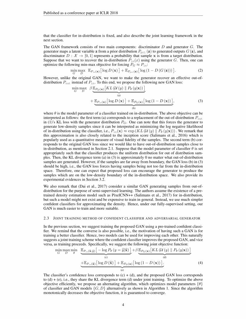
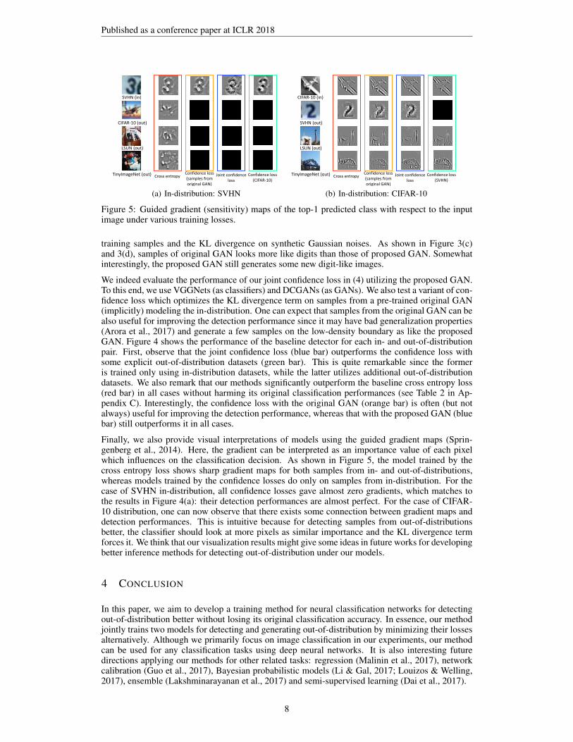
Figure 5: Guided gradient (sensitivity) maps of the top-1 predicted class with respect to the inputimage under various training losses.

training samples and the KL divergence on synthetic Gaussian noises. As shown in Figure 3(c)and 3(d), samples of original GAN looks more like digits than those of proposed GAN. Somewhatinterestingly, the proposed GAN still generates some new digit-like images.

We indeed evaluate the performance of our joint confidence loss in (4) utilizing the proposed GAN.To this end, we use VGGNets (as classifiers) and DCGANs (as GANs). We also test a variant of con-fidence loss which optimizes the KL divergence term on samples from a pre-trained original GAN(implicitly) modeling the in-distribution. One can expect that samples from the original GAN can bealso useful for improving the detection performance since it may have bad generalization properties(Arora et al., 2017) and generate a few samples on the low-density boundary as like the proposedGAN. Figure 4 shows the performance of the baseline detector for each in- and out-of-distributionpair. First, observe that the joint confidence loss (blue bar) outperforms the confidence loss withsome explicit out-of-distribution datasets (green bar). This is quite remarkable since the formeris trained only using in-distribution datasets, while the latter utilizes additional out-of-distributiondatasets. We also remark that our methods significantly outperform the baseline cross entropy loss(red bar) in all cases without harming its original classification performances (see Table 2 in Ap-pendix C). Interestingly, the confidence loss with the original GAN (orange bar) is often (but notalways) useful for improving the detection performance, whereas that with the proposed GAN (bluebar) still outperforms it in all cases.

Finally, we also provide visual interpretations of models using the guided gradient maps (Sprin-genberg et al., 2014). Here, the gradient can be interpreted as an importance value of each pixelwhich influences on the classification decision. As shown in Figure 5, the model trained by thecross entropy loss shows sharp gradient maps for both samples from in- and out-of-distributions,whereas models trained by the confidence losses do only on samples from in-distribution. For thecase of SVHN in-distribution, all confidence losses gave almost zero gradients, which matches tothe results in Figure 4(a): their detection performances are almost perfect. For the case of CIFAR-10 distribution, one can now observe that there exists some connection between gradient maps anddetection performances. This is intuitive because for detecting samples from out-of-distributionsbetter, the classifier should look at more pixels as similar importance and the KL divergence termforces it. We think that our visualization results might give some ideas in future works for developingbetter inference methods for detecting out-of-distribution under our models.

4 CONCLUSION

In this paper, we aim to develop a training method for neural classification networks for detectingout-of-distribution better without losing its original classification accuracy. In essence, our methodjointly trains two models for detecting and generating out-of-distribution by minimizing their lossesalternatively. Although we primarily focus on image classification in our experiments, our methodcan be used for any classification tasks using deep neural networks. It is also interesting futuredirections applying our methods for other related tasks: regression (Malinin et al., 2017), networkcalibration (Guo et al., 2017), Bayesian probabilistic models (Li & Gal, 2017; Louizos & Welling,2017), ensemble (Lakshminarayanan et al., 2017) and semi-supervised learning (Dai et al., 2017).

8


ACKNOWLEDGEMENTS

This work was supported in part by the Institute for Information & communications TechnologyPromotion(IITP) grant funded by the Korea government(MSIT) (No.2017-0-01778, Developmentof Explainable Human-level Deep Machine Learning Inference Framework), the ICT R&D programof MSIP/IITP [R-20161130-004520, Research on Adaptive Machine Learning Technology Devel-opment for Intelligent Autonomous Digital Companion], DARPA Explainable AI (XAI) program#313498 and Sloan Research Fellowship.

REFERENCES

Dario Amodei, Chris Olah, Jacob Steinhardt, Paul Christiano, John Schulman, and Dan Mane. Con-crete problems in ai safety. arXiv preprint arXiv:1606.06565, 2016.

Sanjeev Arora, Rong Ge, Yingyu Liang, Tengyu Ma, and Yi Zhang. Generalization and equilibriumin generative adversarial nets (gans). In International Conference on Machine Learning (ICML),2017.

Rich Caruana, Yin Lou, Johannes Gehrke, Paul Koch, Marc Sturm, and Noemie Elhadad. Intelligiblemodels for healthcare: Predicting pneumonia risk and hospital 30-day readmission. In ACMSIGKDD International Conference on Knowledge Discovery and Data Mining, 2015.

Zihang Dai, Zhilin Yang, Fan Yang, William W Cohen, and Ruslan Salakhutdinov. Good semi-supervised learning that requires a bad gan. In Advances in neural information processing systems(NIPS), 2017.

Jia Deng, Wei Dong, Richard Socher, Li-Jia Li, Kai Li, and Li Fei-Fei. Imagenet: A large-scalehierarchical image database. In Computer Vision and Pattern Recognition (CVPR), 2009.

Ross Girshick. Fast r-cnn. In International Conference on Computer Vision (ICCV), 2015.

Ian Goodfellow, Jean Pouget-Abadie, Mehdi Mirza, Bing Xu, David Warde-Farley, Sherjil Ozair,Aaron Courville, and Yoshua Bengio. Generative adversarial nets. In Advances in neural infor-mation processing systems (NIPS), 2014.

Chuan Guo, Geoff Pleiss, Yu Sun, and Kilian Q Weinberger. On calibration of modern neuralnetworks. In International Conference on Machine Learning (ICML), 2017.

Awni Hannun, Carl Case, Jared Casper, Bryan Catanzaro, Greg Diamos, Erich Elsen, Ryan Prenger,Sanjeev Satheesh, Shubho Sengupta, Adam Coates, et al. Deep speech: Scaling up end-to-endspeech recognition. arXiv preprint arXiv:1412.5567, 2014.

Dan Hendrycks and Kevin Gimpel. A baseline for detecting misclassified and out-of-distributionexamples in neural networks. In International Conference on Learning Representations (ICLR),2016.

Geoffrey E Hinton, Nitish Srivastava, Alex Krizhevsky, Ilya Sutskever, and Ruslan R Salakhutdi-nov. Improving neural networks by preventing co-adaptation of feature detectors. arXiv preprintarXiv:1207.0580, 2012.

Sergey Ioffe and Christian Szegedy. Batch normalization: Accelerating deep network training byreducing internal covariate shift. In International Conference on Machine Learning (ICML), 2015.

Diederik Kingma and Jimmy Ba. Adam: A method for stochastic optimization. In InternationalConference on Learning Representations (ICLR), 2014.

Alex Krizhevsky. One weird trick for parallelizing convolutional neural networks. arXiv preprintarXiv:1404.5997, 2014.

Alex Krizhevsky and Geoffrey Hinton. Learning multiple layers of features from tiny images. 2009.

Balaji Lakshminarayanan, Alexander Pritzel, and Charles Blundell. Simple and scalable predic-tive uncertainty estimation using deep ensembles. In Advances in neural information processingsystems (NIPS), 2017.

9


Yann LeCun, Leon Bottou, Yoshua Bengio, and Patrick Haffner. Gradient-based learning applied todocument recognition. Proceedings of the IEEE, 86(11):2278–2324, 1998.

Kimin Lee, Changho Hwang, KyoungSoo Park, and Jinwoo Shin. Confident multiple choice learn-ing. In International Conference on Machine Learning (ICML), 2017.

Yingzhen Li and Yarin Gal. Dropout inference in bayesian neural networks with alpha-divergences.In International Conference on Machine Learning (ICML), 2017.

Shiyu Liang, Yixuan Li, and R Srikant. Principled detection of out-of-distribution examples inneural networks. arXiv preprint arXiv:1706.02690, 2017.

Christos Louizos and Max Welling. Multiplicative normalizing flows for variational bayesian neuralnetworks. In International Conference on Machine Learning (ICML), 2017.

Andrey Malinin, Anton Ragni, Kate Knill, and Mark Gales. Incorporating uncertainty into deeplearning for spoken language assessment. In Proceedings of the 55th Annual Meeting of theAssociation for Computational Linguistics (Volume 2: Short Papers), volume 2, pp. 45–50, 2017.

Mahdi Pakdaman Naeini, Gregory F Cooper, and Milos Hauskrecht. Obtaining well calibratedprobabilities using bayesian binning. In AAAI, 2015.

Yuval Netzer, Tao Wang, Adam Coates, Alessandro Bissacco, Bo Wu, and Andrew Y Ng. Readingdigits in natural images with unsupervised feature learning. In NIPS workshop on deep learningand unsupervised feature learning, volume 2011, pp. 5, 2011.

Gabriel Pereyra, George Tucker, Jan Chorowski, Łukasz Kaiser, and Geoffrey Hinton. Regularizingneural networks by penalizing confident output distributions. arXiv preprint arXiv:1701.06548,2017.

Alec Radford, Luke Metz, and Soumith Chintala. Unsupervised representation learning with deepconvolutional generative adversarial networks. In International Conference on Learning Repre-sentations (ICLR), 2015.

Tim Salimans, Ian Goodfellow, Wojciech Zaremba, Vicki Cheung, Alec Radford, and Xi Chen.Improved techniques for training gans. In Advances in neural information processing systems(NIPS), 2016.

Tim Salimans, Andrej Karpathy, Xi Chen, and Diederik P Kingma. Pixelcnn++: Improving thepixelcnn with discretized logistic mixture likelihood and other modifications. In InternationalConference on Learning Representations (ICLR), 2017.

Ashish Shrivastava, Tomas Pfister, Oncel Tuzel, Josh Susskind, Wenda Wang, and Russ Webb.Learning from simulated and unsupervised images through adversarial training. In ComputerVision and Pattern Recognition (CVPR), 2017.

Jost Tobias Springenberg, Alexey Dosovitskiy, Thomas Brox, and Martin Riedmiller. Striving forsimplicity: The all convolutional net. arXiv preprint arXiv:1412.6806, 2014.

Christian Szegedy, Wei Liu, Yangqing Jia, Pierre Sermanet, Scott Reed, Dragomir Anguelov, Du-mitru Erhan, Vincent Vanhoucke, and Andrew Rabinovich. Going deeper with convolutions. InComputer Vision and Pattern Recognition (CVPR), 2015.

Ruben Villegas, Jimei Yang, Yuliang Zou, Sungryull Sohn, Xunyu Lin, and Honglak Lee. Learningto generate long-term future via hierarchical prediction. In International Conference on MachineLearning (ICML), 2017.

Fisher Yu, Ari Seff, Yinda Zhang, Shuran Song, Thomas Funkhouser, and Jianxiong Xiao. Lsun:Construction of a large-scale image dataset using deep learning with humans in the loop. arXivpreprint arXiv:1506.03365, 2015.

Junbo Zhao, Michael Mathieu, and Yann LeCun. Energy-based generative adversarial network. InInternational Conference on Learning Representations (ICLR), 2017.

10


A THRESHOLD-BASED DETECTORS

In this section, we formally describe the detection procedure of threshold-based detectors(Hendrycks & Gimpel, 2016; Liang et al., 2017). For each data x, it measures some confidencescore q(x) by feeding the data into a pre-trained classifier. Here, (Hendrycks & Gimpel, 2016) de-fined the confidence score as a maximum value of the predictive distribution, and (Liang et al., 2017)further improved the performance by processing the predictive distribution (see Appendix C.3 formore details). Then, the detector, g (x) : X → {0, 1}, assigns label 1 if the confidence score q(x) isabove some threshold δ, and label 0, otherwise:

g (x) =

{1 if q(x) ≥ δ,0 otherwise.

For this detector, we have to find a score threshold so that some positive examples are classifiedcorrectly, but this depends upon the trade-off between false negatives and false positives. To handlethis issue, we use threshold-independent evaluation metrics such as area under the receiver operatingcharacteristic curve (AUORC) and detection accuracy (see Appendix B).

B EXPERIMENTAL SETUPS IN SECTION 3

Datasets. We train deep models such as VGGNet (Szegedy et al., 2015) and AlexNet (Krizhevsky,2014) for classifying CIFAR-10 and SVHN datasets: the former consists of 50,000 training and10,000 test images with 10 image classes, and the latter consists of 73,257 training and 26,032 testimages with 10 digits.2 The corresponding test dataset are used as the in-distribution (positive)samples to measure the performance. We use realistic images and synthetic noises as the out-of-distribution (negative) samples: the TinyImageNet consists of 10,000 test images with 200 imageclasses from a subset of ImageNet images. The LSUN consists of 10,000 test images of 10 differentscenes. We downsample each image of TinyImageNet and LSUN to size 32 × 32. The Gaussiannoise is independently and identically sampled from a Gaussian distribution with mean 0.5 andvariance 1. We clip each pixel value into the range [0, 1].

Detailed CNN structure and training. The simple CNN that we use for evaluation shown in Figure2 consists of two convolutional layers followed by three fully-connected layers. Convolutional layershave 128 and 256 filters, respectively. Each convolutional layer has a 5 × 5 receptive field appliedwith a stride of 1 pixel each followed by max pooling layer which pools 2 × 2 regions at strides of2 pixels. AlexNet (Krizhevsky, 2014) consists of five convolutitonal layers followed by three fully-connected layers. Convolutional layers have 64, 192, 384, 256 and 256 filters, respectively. First andsecond convolutional layers have a 5×5 receptive field applied with a stride of 1 pixel each followedby max pooling layer which pools 3 × 3 regions at strides of 2 pixels. Other convolutional layershave a 3 × 3 receptive field applied with a stride of 1 pixel followed by max pooling layer whichpools 2 × 2 regions at strides of 2 pixels. Fully-connected layers have 2048, 1024 and 10 hiddenunits, respectively. Dropout (Hinton et al., 2012) was applied to only fully-connected layers of thenetwork with the probability of retaining the unit being 0.5. All hidden units are ReLUs. Figure6 shows the detailed structure of VGGNet (Szegedy et al., 2015) with three fully-connected layersand 10 convolutional layers. Each ConvReLU box in the figure indicates a 3× 3 convolutional layerfollowed by ReLU activation. Also, all max pooling layers have 2× 2 receptive fields with stride 2.Dropout was applied to only fully-connected layers of the network with the probability of retainingthe unit being 0.5. For all experiments, the softmax classifier is used, and each model is trained byoptimizing the objective function using Adam learning rule (Kingma & Ba, 2014). For each out-of-distribution dataset, we randomly select 1,000 images for tuning the penalty parameter β, mini-batchsize and learning rate. The penalty parameter is chosen from β ∈ {0, 0.1, . . . 1.9, 2}, the mini-batchsize is chosen from {64, 128} and the learning rate is chosen from {0.001, 0.0005, 0.0002}. Theoptimal parameters are chosen to minimize the detection error on the validation set. We drop thelearning rate by 0.1 at 60 epoch and models are trained for total 100 epochs. The best test result isreported for each method.

Performance metrics. We measure the following metrics using threshold-based detectors:

2We do not use the extra SVHN dataset for training.

11


• True negative rate (TNR) at 95% true positive rate (TPR). Let TP, TN, FP, and FN de-note true positive, true negative, false positive and false negative, respectively. We measureTNR = TN / (FP+TN), when TPR = TP / (TP+FN) is 95%.• Area under the receiver operating characteristic curve (AUROC). The ROC curve is a

graph plotting TPR against the false positive rate = FP / (FP+TN) by varying a threshold.• Area under the precision-recall curve (AUPR). The PR curve is a graph plotting the

precision = TP / (TP+FP) against recall = TP / (TP+FN) by varying a threshold. AUPR-IN(or -OUT) is AUPR where in- (or out-of-) distribution samples are specified as positive.• Detection accuracy. This metric corresponds to the maximum classification proba-

bility over all possible thresholds δ: 1 − minδ{Pin (q (x) ≤ δ)P (x is from Pin) +

Pout (q (x) > δ)P (x is from Pout)}, where q(x) is a confident score such as a maxi-

mum value of softmax. We assume that both positive and negative examples have equalprobability of appearing in the test set, i.e., P (x is from Pin) = P (x is from Pout) = 0.5.

Note that AUROC, AUPR and detection accuracy are threshold-independent evaluation metrics.

FC (

51

2)

Co

nvR

eLU

(64

f.m

aps)

max

po

ol

Co

nvR

eLU

(64

f.m

aps)

Co

nvR

eLU

(25

6 f

.map

s)

Co

nvR

eLU

(25

6 f

.map

s)

max

po

ol

Co

nvR

eLU

(12

8 f

.map

s)

max

po

ol

Co

nvR

eLU

(12

8 f

.map

s)

Co

nvR

eLU

(51

2 f

.map

s)

Co

nvR

eLU

(51

2 f

.map

s)

max

po

ol

Co

nvR

eLU

(51

2 f

.map

s)

Co

nvR

eLU

(51

2 f

.map

s)

avg

po

ol

FC (

10

)

FC (

51

2)

Figure 6: Detailed structure of VGGNet with 13 layers.

Generating samples on a simple example. As shown in Figure 3(a) and Figure 3(b), we comparethe generated samples by original GAN and proposed GAN on a simple example where the targetdistribution is a mixture of two Gaussian distributions. For both the generator and discriminator, weuse fully-connected neural networks with 2 hidden layers and 500 hidden units for each layer. Forall layers, we use ReLU activation function. We use a 100-dimensional Gaussian prior for the latentvariable z. For our method, we pre-train the simple fully-connected neural networks (2 hidden layersand 500 ReLU units for each layer) by minimizing the cross entropy on target distribution samplesand the KL divergence on out-of-distribution samples generated by rejection sampling on bounded2D box [−10, 10]2. The penalty parameter β is set to 1. We use ADAM learning rule (Kingma &Ba, 2014) with a mini-batch size of 400. The initial learning rate is set to 0.002, and we train fortotal 100 epochs.

Generating samples on MNIST. As shown in Figure 3(c) and Figure 3(d), we compare the gener-ated samples of original and proposed GANs on MNIST dataset, which consists of greyscale images,each containing a digit 0 to 9 with 60,000 training and 10,000 test images. We expand each imageto size 3 × 32 × 32. For both the generator and discriminator, we use deep convolutional GANs(DCGANs) (Radford et al., 2015). The discriminator and generator consist of four convolutionaland deconvolutional layers, respectively. Convolutional layers have 128, 256, 512 and 1 filters, re-spectively. Each convolutional layer has a 4× 4 receptive field applied with a stride of 2 pixel. Thesecond and third convolutional layers are followed by batch normalization (Ioffe & Szegedy, 2015).For all layers, we use LeakyReLU activation function. Deconvolutional layers have 512, 256, 128and 1 filters, respectively. Each deconvolutional layer has a 4 × 4 receptive field applied with astride of 2 pixel followed by batch normalization (Ioffe & Szegedy, 2015) and ReLU activation.For our method, we use a pre-trained simple CNNs (two convolutional layers followed by threefully-connected layers) by minimizing the cross entropy on MNIST training samples and the KLdivergence on synthetic Gaussian noise. Convolutional layers have 128 and 256 filters, respectively.Each convolutional layer has a 5× 5 receptive field applied with a stride of 1 pixel each followed bymax pooling layer which pools 2 × 2 regions at strides of 2 pixels. The penalty parameter β is setto 1. We use ADAM learning rule (Kingma & Ba, 2014) with a mini-batch size of 128. The initiallearning rate is set to 0.0002, and we train for total 50 epochs.

12


C MORE EXPERIMENTAL RESULTS

C.1 CLASSIFICATION PERFORMANCES

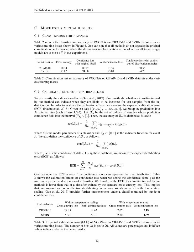
Table 2 reports the classification accuracy of VGGNets on CIFAR-10 and SVHN datasets undervarious training losses shown in Figure 4. One can note that all methods do not degrade the originalclassification performance, where the differences in classification errors of across all tested singlemodels are at most 1% in our experiments.

In-distribution Cross entropy Confidence losswith original GAN Joint confidence loss Confidence loss with explicit

out-of-distribution samples

CIFAR-10 80.14 80.27 81.39 80.56SVHN 93.82 94.08 93.81 94.23

Table 2: Classification test set accuracy of VGGNets on CIFAR-10 and SVHN datasets under vari-ous training losses.

C.2 CALIBRATION EFFECTS OF CONFIDENCE LOSS

We also verify the calibration effects (Guo et al., 2017) of our methods: whether a classifier trainedby our method can indicate when they are likely to be incorrect for test samples from the in-distribution. In order to evaluate the calibration effects, we measure the expected calibration error(ECE) (Naeini et al., 2015). Given test data {(x1, y1) , . . . , (xn, yn)}, we group the predictions intoM interval bins (each of size 1/M ). Let Bm be the set of indices of samples whose predictionconfidence falls into the interval (m−1M , mM ]. Then, the accuracy of Bm is defined as follows:

acc(Bm) =1

|Bm|∑i∈Bm

1{yi=argmaxy

Pθ(y|xi)},

where θ is the model parameters of a classifier and 1A ∈ {0, 1} is the indicator function for eventA. We also define the confidence of Bm as follows:

conf(Bm) =1

|Bm|∑i∈Bm

q(xi),

where q(xi) is the confidence of data i. Using these notations, we measure the expected calibrationerror (ECE) as follows:

ECE =

M∑m=1

|Bm|n|acc(Bm)− conf(Bm)|.

One can note that ECE is zero if the confidence score can represent the true distribution. Table3 shows the calibration effects of confidence loss when we define the confidence score q as themaximum predictive distribution of a classifier. We found that the ECE of a classifier trained by ourmethods is lower than that of a classifier trained by the standard cross entropy loss. This impliesthat our proposed method is effective at calibrating predictions. We also remark that the temperaturescaling (Guo et al., 2017) provides further improvements under a classifier trained by our jointconfidence loss.

In-distribution Without temperature scaling With temperature scalingCross entropy loss Joint confidence loss Cross entropy loss Joint confidence loss

CIFAR-10 18.45 14.62 7.07 6.19SVHN 5.30 5.13 2.80 1.39

Table 3: Expected calibration error (ECE) of VGGNets on CIFAR-10 and SVHN datasets undervarious training losses. The number of bins M is set to 20. All values are percentages and boldfacevalues indicate relative the better results.

13


C.3 EXPERIMENTAL RESULTS USING ODIN DETECTOR

In this section, we verify the effects of confidence loss using ODIN detector (Liang et al., 2017)which is an advanced threshold-based detector using temperature scaling (Guo et al., 2017) andinput perturbation. The key idea of ODIN is the temperature scaling which is defined as follows:

Pθ(y = y|x;T ) =exp (fy(x)/T )∑y exp (fy(x)/T )

,

where T > 0 is the temperature scaling parameter and f = (f1, . . . , fK) is final feature vector ofneural networks. For each data x, ODIN first calculates the pre-processed image x by adding thesmall perturbations as follows:

x′ = x− εsign (−5x logPθ(y = y|x;T )) ,where ε is a magnitude of noise and y is the predicted label. Next, ODIN feeds the pre-processed data into the classifier, computes the maximum value of scaled predictive distribution,i.e., maxy Pθ(y|x′;T ), and classifies it as positive (i.e., in-distribution) if the confidence score isabove some threshold δ.

For ODIN detector, the perturbation noise ε is chosen from {0, 0.0001, 0.001, 0.01}, and the tem-perature T is chosen from {1, 10, 100, 500, 1000}. The optimal parameters are chosen to minimizethe detection error on the validation set. Figure 7 shows the performance of the OIDN and baselinedetector for each in- and out-of-distribution pair. First, we remark that the baseline detector usingclassifiers trained by our joint confidence loss (blue bar) typically outperforms the ODIN detec-tor using classifiers trained by the cross entropy loss (orange bar). This means that our classifiercan map in- and out-of-distributions more separately without pre-processing methods such as tem-perature scaling. The ODIN detector provides further improvements if one uses it with our jointconfidence loss (green bar). In other words, our proposed training method can improve all priordetection methods.

Crossentropyloss + ODIN Jointconfidenceloss+ ODINCrossentropyloss + baseline Jointconfidenceloss+ baseline

40

50

60

70

80

90

100

TNR at TPR 95%


Out-of-distribution: CIFAR-10

40

50

60

70

80

90

100

TNR at TPR 95%



40

50

60

70

80

90

100

TNR at TPR 95%




0102030405060708090

100

TNR TPR 95%


Out-of-distribution: SVHN

0102030405060708090

100

TNR at TPR 95%



0102030405060708090

100

TNR at TPR 95%




Figure 7: Performances of the baseline detector (Hendrycks & Gimpel, 2016) and ODIN detector(Liang et al., 2017) under various training losses.

C.4 EXPERIMENTAL RESULTS ON ALEXNET

Table 4 shows the detection performance for each in- and out-of-distribution pair when the classifieris AlexNet (Krizhevsky, 2014), which is one of popular CNN architectures. We remark that theyshow similar trends.

14



accuracyTNR


AUPRin

AUPRout

Cross entropy loss / Confidence loss

Baseline(SVHN)

CIFAR-10 (seen)

92.14 / 93.77



Baseline(CIFAR-10)

SVHN (seen)

76.58 / 76.18



ODIN(SVHN)

CIFAR-10 (seen)

92.14 / 93.77



ODIN(CIFAR-10)

SVHN (seen)

76.58 / 76.18



Table 4: Performance of the baseline detector (Hendrycks & Gimpel, 2016) and ODIN detector(Liang et al., 2017) using AlexNet. All values are percentages and boldface values indicate rela-tive the better results. For each in-distribution, we minimize the KL divergence term in (1) usingtraining samples from an out-of-distribution dataset denoted by “seen”, where other “unseen” out-of-distributions were also used for testing.

D MAXIMIZING ENTROPY

One might expect that the entropy of out-of-distribution is expected to be much higher compared tothat of in-distribution since the out-of-distribution is typically on a much larger space than the in-distribution. Therefore, one can add maximizing the entropy of generator distribution to new GANloss in (3) and joint confidence loss in (4). However, maximizing the entropy of generator distribu-tion is technically challenging since a GAN does not model the generator distribution explicitly. Tohandle the issue, one can leverage the pull-away term (PT) (Zhao et al., 2017):

−H (PG (x)) w PT (PG (x)) =1

M(M − 1)

M∑i=1

∑j 6=i

(G (zi)

>G (zj)

‖G (zi)‖‖G (zj)‖

)2

,

where H (·) denotes the entropy, zi, zj ∼ Ppri (z) and M is the number of samples. Intuitively,one can expect the effect of increasing the entropy by minimizing PT since it corresponds to thesquared cosine similarity of generated samples. We note that (Dai et al., 2017) also used PT tomaximize the entropy. Similarly as in Section 3.2, we verify the effects of PT using VGGNet. Table5 shows the performance of the baseline detector for each in- and out-of-distribution pair. We foundthat joint confidence loss with PT tends to (but not always) improve the detection performance.However, since PT increases the training complexity and the gains from PT are relatively marginal(or controversial), we leave it as an auxiliary option for improving the performance.


accuracyTNR


AUPRin

AUPRout

Joint confidence loss without PT / with PT

SVHNCIFAR-10

93.81 / 94.0590.1 / 92.3 97.6 / 98.1 93.6 / 94.6 97.7 / 98.2 97.9 / 98.7

TinyImageNet 99.0 / 99.9 99.6 / 100.0 97.6 / 99.7 99.7 / 100.0 94.5 / 100.0LSUN 98.9 / 100.0 99.6 / 100.0 97.5 / 99.9 99.7 / 100.0 95.5 / 100.0

CIFAR-10SVHN

81.39 / 80.6025.4 / 13.2 66.8 / 69.5 74.2 / 75.1 71.3 / 73.5 78.3 / 72.0

TinyImageNet 35.0 / 44.8 72.0 / 78.4 76.4 / 77.6 74.7 / 79.4 82.2 / 84.4LSUN 39.1 / 49.1 75.1 / 80.7 77.8 / 78.7 77.1 / 81.3 83.6 / 85.8

Table 5: Performance of the baseline detector (Hendrycks & Gimpel, 2016) using VGGNets trainedby joint confidence loss with and without pull-away term (PT). All values are percentages and bold-face values indicate relative the better results.

15


E ADDING OUT-OF-DISTRIBUTION CLASS

Instead of forcing the predictive distribution on out-of-distribution samples to be closer to the uni-form one, one can simply add an additional “out-of-distribution” class to a classifier as follows:

minθ

EPin(x,y)


]+ EPout(x)

[− logPθ (y = K + 1|x)

], (5)

where θ is a model parameter. Similarly as in Section 3.1, we compare the performance of theconfidence loss with that of above loss in (5) using VGGNets with for image classification on SVHNdataset. To optimize the KL divergence term in confidence loss and the second term of (5), CIFAR-10 training datasets are used. In order to compare the detection performance, we define the theconfidence score of input x as 1 − Pθ (y = K + 1|x) in case of (5). Table 6 shows the detectionperformance for out-of-distribution. First, the classifier trained by our method often significantlyoutperforms the alternative adding the new class label. This is because modeling explicitly out-of-distribution can incur overfitting to trained out-of-distribution dataset.

Detector Out-of-distClassification

accuracyTNR


AUPRin

AUPRout

K + 1 class loss in (5) / Confidence loss

Baselinedetector

SVHN (seen)

79.61 / 80.56



ODINdetector

SVHN (seen)

79.61 / 80.56



Table 6: Performance of the baseline detector (Hendrycks & Gimpel, 2016) and ODIN detector(Liang et al., 2017) using VGGNet. All values are percentages and boldface values indicate relativethe better results.

16

Documents

TRAINING CONFIDENCE CALIBRATED CLASSIFIERS FOR …