Trading Population for Productivity: Theory and Evidence

Oded Galor and Andrew Mountford�

January 21, 2008

Abstract

This research argues that the di¤erential e¤ect of international trade on the demand for human capitalacross countries has been a major determinant of the distribution of income and population across theglobe. In developed countries the gains from trade have been directed towards investment in educationand growth in income per capita, whereas a signi�cant portion of these gains in less developed economieshave been channeled towards population growth. Cross-country regressions establish that indeed tradehas positive e¤ects on fertility and negative e¤ects on education in non-OECD economies, while inducingfertility decline and human capital formation in OECD economies.

Keywords: International Trade , Demographic Transition, Growth, Human Capital

JEL Classi�cation Numbers: O40, F11, F43, J10, N30

�The authors are grateful to the Editor, three referees, and Yona Rubinstein for their extensive valuable comments. Inaddition, they wish to thank Daron Acemoglu, Quamrul Ashraf, Anne Case, Francesco Caselli, Ronald Findlay, Gene Grossman,Elhanan Helpman, Wolfgang Keller, Joel Mokyr, Enrico Spolaore, David Weil, Je¤Williamson and seminar participants at Bern,Birmingham, Brown, Columbia, Harvard, Kent, Penn, Princeton, Royal Institute for International A¤airs, Royal Holloway,University of London, Southampton, Tel-Aviv, and conference participants at the CEPR ERWIT, Munich, AEA Meetings,Minerva�s Conference �From Stagnation to Growth�, Economic Growth in the Very Long Run, Copenhagen, and NBER SummerInstitute, for helpful comments. Galor: Brown University. Mountford: Royal Holloway, University of London. Galor�s researchis supported by NSF grant SES-0004304.

0

1 Introduction

The dramatic transformation in the distribution of income and population across the globe in the past two

centuries is one of the most signi�cant mysteries in the growth process. Some regions have excelled in the

growth of income per capita while other regions have been dominant in population growth.1 How does one

account for the sudden take-o¤ from stagnation to growth in some countries in the world and the persistent

stagnation in others? Why have the di¤erences in per capita incomes across countries increased so markedly

in the last two centuries? What accounts for the di¤erential timing of the demographic transition across

countries? Has the pace of transition to sustained economic growth in advanced economies adversely a¤ected

the process of development in less-developed economies?

The origin of this �Great Divergence�has been a source of controversy. The relative roles of geograph-

ical and institutional factors, human capital formation, ethnic, linguistic and religious fractionalization,

colonialism and globalization have been at the center of a debate about this remarkable change in the world

income distribution in the past two centuries.2

This research suggests that international trade has played a signi�cant role in the di¤erential timing

of demographic transitions across countries and has been a major determinant of the distribution of world

population and the �Great Divergence�in income per capita across countries in the last two centuries. The

analysis suggests that international trade has an asymmetrical e¤ect on the evolution of industrial and non-

industrial economies. While in the industrial nations the gains from trade have been directed primarily

towards investment in education and growth in output per capita, a greater portion of the gains from trade

in non-industrial nations has been channeled towards population growth.

The expansion of international trade in the second phase of the Industrial Revolution enhanced the

specialization of industrial economies in the production of industrial, skilled intensive, goods. The associ-

ated rise in the demand for skilled labor has induced a gradual investment in the quality of the population,

expediting a demographic transition, stimulating technological progress and further enhancing the compar-

ative advantage of these industrial economies in the production of skilled intensive goods. In non-industrial

economies, in contrast, international trade has generated an incentive to specialize in the production of un-

skilled intensive, non-industrial, goods. The absence of signi�cant demand for human capital has provided

limited incentives to invest in the quality of the population and the gains from trade have been utilized pri-

marily for a further increase in the size of the population, rather than the income of the existing population.3

1 In the time period 1820-1998, the ratio between income per capita in the richest region of the world and the poorest regionof the world has increased from about 3 to 19. In particular, the ratio between income per capita in Western Europe and Asiagrew nearly three-fold, whereas the ratio between the Asian population and the Western European population grew nearlytwo-fold (Maddison, 2001).

2North (1981), Landes (1998), Mokyr (2002), Hall and Jones (1999), Acemoglu, et al. (2005), Easterly and Levine (2003),Rodrik, et al. (2004) and Ashraf and Galor (2007) have argued that institutions that facilitated the protection of property rightsand enhanced technological research, the di¤usion of knowledge, and the transmission of society speci�c human capital, havebeen the prime factors that enabled the earlier European take-o¤ and the great technological divergence across the globe. Thee¤ect of geographical factors on economic growth and the great divergence have been emphasized by Jones (1981), Diamond(1997), Gallup, Sachs and Mellinger (1998) and Pomeranz (2000). Finally, the role of human capital in the great divergenceis underlined in uni�ed growth theory (Galor, 2005; Galor and Weil 2000; Galor and Moav, 2002; McDermott, 2002; Doepke,2004; Lagerlof, 2006; Galor et al., 2006) and is documented empirically by Glaeser et al. (2004).

3Evidence suggests that the returns to human capital may have been higher in LDCs. One can therefore mistakenlysuppose that incentive to invest in child quality is higher in LDCs. However, these higher rates of return are not applicable

1

The demographic transition in these non-industrial economies has been signi�cantly delayed, increasing fur-

ther their relative abundance of unskilled labor, enhancing their comparative disadvantage in the production

of skilled intensive goods and delaying their process of development. The research suggests, therefore, that

international trade has persistently a¤ected the distribution of population, skills, and technologies in the

world economy, and has been a signi�cant force behind the �Great Divergence�in income per capita across

countries.

This paper develops a uni�ed growth theory that captures the asymmetric role that international trade

may have played in expediting the transition to sustained economic growth in technologically advanced

economies and in delaying the transition in technologically inferior economies. The proposed theory is

innovative in two dimensions. First, unlike the recent literature on the transition of economies from an

epoch of Malthusian stagnation to a state of sustained economic growth that abstracted from the Great

Divergence and focused on the evolution of the world economy from stagnation to growth,4 the proposed

theory examines the di¤erential patterns of takeo¤s across regions in the world and the emergence of the

Great Divergence. Second, in contrast to the existing literature on the dynamics of comparative advantage,5

the focus on the interaction between population growth and comparative advantage and the persistent e¤ect

that this interaction may have on the distribution of population and income in the world economy generates

an important new insight regarding the distribution of the gains from trade. The theory suggests that even

if trade equalizes output growth in the trading countries, (due to the terms of trade e¤ect), income per capita

of developed and less developed economies will diverge, since in developed economies the growth of total

output will be generated primarily by an increase in output per capita, whereas in less developed economies

the contribution of population growth to the growth of total output will be more signi�cant.6

The theory is based on several fundamental elements. The interaction between these elements gener-

ates a dynamic pattern that is consistent with the observed asymmetrical evolution of the world economy

from the epoch of Malthusian stagnation to the current era of sustained growth, characterized by widened

di¤erences in income per capita and population growth rates, as well as by persistent patterns of compar-

ative advantage. Economies are initially in a Malthusian epoch in which the growth rate of output per

capita is rather small and population growth is positively related to the level of income per capita. Techno-

logical progress leads ultimately to the adoption of more advanced agricultural and industrial technologies

which paves the way for the take-o¤ from the Malthusian epoch. International trade induces technologi-

cally advanced economies to specialize in the production of skilled intensive manufactured goods whereas

to most individuals. They re�ect a suboptimal investment in human capital in an environment characterized by credit marketimperfections and limited access to schooling. International trade, therefore reduces further the modest demand for humancapital and reduces further the incentive to substitute child quality for quantity.

4 In particular, Galor and Weil (1999, 2000) argue that the inherent positive interaction between population and technologyduring the Malthusian regime increased the rate of technological progress su¢ ciently so as to induce investment in humancapital which led to further technological progress, a demographic transition, and sustained economic growth.

5See Findlay and Kierzkowski (1983), Grossman and Helpman (1991), Matsuyama (1992), Young (1991) and Atkeson andKehoe (2000), among others.

6See, for example, Acemoglu and Ventura (2002) for the terms of trade e¤ect. Deardor¤ (1994) suggests that diverging(exogenous) population growth rates can lead to widening international inequality. Similarly, Krugman and Venables (1995)and Baldwin et al. (2001) argue that the reduction in transportation costs and the associated expansion in trade, generatedgeographically based industrialization and divergence.

2

technologically inferior economies specialize in the production of unskilled intensive agricultural goods. The

increase in the demand for human capital in the technologically advanced economies that is brought about

by international trade induces investment in human capital7 and expedites the demographic transition,8

whereas the reduction in the demand for human capital in less advanced economies delays the demographic

transition and investment in human capital.9

The analysis demonstrates that the acceleration of the demographic transition in the technologically

advanced economies increases their formation of human capital and brings about sustained technological

progress that enhances their comparative advantage in the production of skilled intensive industrial goods.10

In contrast, the delay in the demographic transition in the less advanced economies increases the supply of

unskilled workers and enhances the comparative advantage of these economies in the production of unskilled

intensive goods. Thus, consistent with the evidence provided in sections 5 and 6, the pattern of international

trade has reinforced the initial patterns of comparative advantage and has generated a persistent e¤ect on

the distribution of population in the world economy and a great divergence in income per capita across

countries and regions.

The fundamental hypothesis is tested empirically using contemporary cross country data. In accor-

dance with the theory, cross country regressions support the hypothesis that international trade generates

opposing e¤ects on fertility rates in developed and less developed economies. The analysis establishes that

a larger share of trade in GDP per capita has a positive e¤ect on fertility and a negative e¤ect on human

capital formation in non-OECD economies, whereas in OECD economies, trade triggers a decline in fertility

and an increase in human capital accumulation.

2 An Autarkic Economy

This section analyzes the path of a closed economy from its Malthusian pre-industrial state through a

transitional state of increased fertility, investment in human capital and economic growth to a modern state

with high investment in human capital, low population growth, and sustained economic growth.11

Consider an overlapping-generations economy in which economic activity extends over in�nite discrete

7Consistent with empirical evidence, the increased demand for human capital has not resulted necessarily in an increase inthe equilibrium rate of return to human capital due to a massive supply response generated by (a) the increase in the incentivefor investment in education (for a given cost), and (b) institutional changes (e.g., the provision of public education) that loweredthe cost of investment in human capital.

8Unlike Becker (1981)�s hypothesis where a high level of income induces parents to switch to having fewer, higher qualitychildren, the substitution of quality for quantity is in response to technological progress. The fact that demographic transitionsoccurred around the same period in Western European countries that di¤ered in their income per capita, but shared a similarpattern of future technological progress, supports our technological approach.

9Moreover, the increased specialization of production within an economy would result, ceteris paribus, in increased incomeand fertility inequality within the economy, in line with the �nding of Haines (2000) that fertility rate in rural areas remainedhigher than for urban areas for signi�cant periods in the nineteenth century in both the US and UK, as well as with the �ndingsof de la Croix and Doepke (2003) that income inequality causes di¤erential fertility patterns within and across economies.10Similarly to this element in the theory, Grossman and Helpman (1991) demonstrates that a country that begins with a

head start in the accumulation of knowledge often leads in productivity over time.11Galor and Mountford (2006) abstracts from these stages of development and demonstrates in a simpler Ricardian model

that although international trade may equalize the growth rates of the value of total output in the two trading economies, sincethe rate of population growth in the technologically regressed economy is higher than that in the advanced economy, the rate ofgrowth of output per capita in the technologically advanced economy will be higher than that in the technologically regressedeconomy.

3

time. In every period t; two goods, a manufactured good, Y mt ; and an agricultural good Yat , may be produced

using up to three factors of production, skilled labor, Ht, unskilled labor, Lt; and land, X. The supply of

skilled and unskilled labor is endogenously determined and evolves over time, whereas the quantity of land

is exogenously determined and remains constant over time.12

2.1 Production

In each of the sectors of the economy production may take place with either an old technology or a new one.

In early stages of development the new production technologies are latent and production is conducted using

the old technologies. However, in the process of development the productivity of the new technologies grows

faster than those of the old technologies and ultimately the new technologies become economically viable.

In the agricultural sector, the introduction of the new technology represents the escape from the Malthusian

trap, where wages do not fall despite an increase in population. In the industrial sector, the introduction of

the new technology re�ects an increase in the skill-intensity of the production process in the second phase

of the industrial revolution and the associated increase in the demand for human capital.

2.1.1 Production of the Agricultural Good

The agricultural good can be produced by either an old technology or a new one. The output of the

agricultural good produced with the old technology in period t, Y a;0t ; is

Y a;0t = aat (La;0t ) X1� ; 0 < < 1; (1)

where La;0t is the amount of unskilled labor and X is the amount of land, employed in period t in the

production of the agricultural good using the old technology, and aat is the level of productivity of the old

technology in period t. For simplicity the amount of land is normalized such that X = 1.

The output of the agricultural good produced with the new technology in period t, Y a;Nt ; is governed

by a constant returns to scale production technology13

Y a;Nt = AatLa;Nt ; (2)

where La;Nt is the amount of unskilled labor employed in the production of the agricultural good in period t

using the new technology, and Aat is the level of productivity of the new agricultural technology in period t.

As will become apparent, in the early stages of development when the productivity of the new agri-

cultural technology, Aat ; is low relative to the productivity of the old technology, aat ; only the old technology

will be employed. However in later stages of development, when Aat rises su¢ ciently relative to aat ; the new

agricultural technology becomes economically viable.

2.1.2 Production of the Manufactured Good

The manufactured good can be produced by either an old technology or a new one. The output of the

manufactured good produced with the old technology in period t, Y m;0t ; is

Y m;0t = amt Lm;0t ; (3)

12Since the fundamental mechanism explored in this paper focuses on the role of human capital accumulation and thedemographic transition in the process of development, the abstraction from the role of physical capital is a natural simplifyingassumption.13This production function is designed to capture the decline in the importance of land in mature state of development.

However, as established in Appendix B, the qualitative analysis would remain intact if the agricultural technology remainsland-intensive.

4

where Lm;0t is the amount of unskilled labor employed in period t in the production of the manufactured

good using the old technology, and amt is the level of productivity of the old industrial technology in period

t.

The output of the manufactured good produced with the modern technology in period t, Y m;Nt ; is

governed by a neoclassical constant returns to scale production function,

Y m;Nt = Amt F (Hmt ; L

m;Nt ) = Amt f(h

mt )L

m;Nt ; (4)

where hmt �Hmt =L

m;Nt , Amt is the level of productivity of the new industrial technology in period t, and L

m;Nt

and Hmt are the amounts of unskilled labor and skilled labor employed in the production of the industrial

good in period t using the new technology.

As established below, in the early stages of development when the technological level Amt is low relative

to amt only the old industrial technology is economically viable. However in the process of development as Amt

rises su¢ ciently relative to amt ; it becomes pro�table for producers to employ the new industrial technology.

2.1.3 Factor Prices and Goods�Prices

Producers operate in perfectly competitive markets for �nal goods and for labor. In the absence of property

rights to land, the return to land is zero and workers in the agricultural sector who use the old technology

receive their average products.14

The inverse demand for unskilled labor in the agricultural sector, given (1) and (2), is therefore

wut =

8<:pta

at (L

a;0t ) �1 if Y a;0t > 0

ptAat if Y a;Nt > 0;

(5)

where wut is the wage of an unskilled labor in terms of the manufactured good, and pt as the relative price

of the agricultural good in terms of the manufactured good in period t.

The inverse demand for skilled and unskilled labor in the manufactured sector, given (3) and (4), is

therefore

wut =

8<:amt if Y m;0t > 0

Amt [f(hmt )� hmt f 0(hmt )] � Amt wu(hmt ) if Y m;Nt > 0;

(6)

and

wst = Amt f0(hmt ) � Amt ws(hmt ) if Y m;Nt > 0: (7)

Moreover,wstwut=

f 0(hmt )f(hmt )�hmt f 0(hmt )

� !(hmt ) if Y m;Nt > 0; (8)

where as follows from the neoclassical properties of f(hmt ); !0(hmt ) < 0; limh!0 !(h

mt )!1; and limh!1 !(h

mt ) =

0:

Since unskilled workers are mobile between the agricultural and the industrial sectors, the wages of

unskilled labor in both sectors are equal if both goods are produced. As follows from (5) and (6), pt; the

14See Galor and Weil (2000) for a discussion of alternative formulations in which property rights for land are present.

5

relative price of the agricultural good in terms of the manufactured good in period t, is therefore

pt =

8>>>>>>>>>>><>>>>>>>>>>>:

amtaat (L

a;0t ) �1

if Y a;0t > 0 and Y m;0t > 0

amtAat

if Y a;Nt > 0 and Y m;0t > 0

Amt w

u(hmt )

aat (La;0t ) �1

if Y a;0t > 0 and Y m;Nt > 0

Amt w

u(hmt )Aat

if Y a;Nt > 0 and Y m;Nt > 0:

(9)

2.2 Individuals: Fertility, Human Capital and Consumption

Individuals live for two periods. In their �rst period of life they consume a fraction of their parental unit

time endowment; educated o¤spring require a larger fraction of parental time. In their second period of

life they are endowed with one unit of time of either skilled, s; or unskilled labor, u; which they optimally

allocate between child rearing and labor force participation.

2.2.1 Preferences and Budget Constraints

Individual�s preferences are de�ned over consumption and the potential aggregate income of their children.15

The preferences of a member i; i = s; u; of generation t (i.e. an individual who is born in period t � 1) arerepresented by the utility function

ut = (ci;at )

�(ci;mt )� [wst+1ni;st + wut+1n

i;ut ]

1���� ; (10)

where ci;at and ci;mt are individual i�s consumption of the agricultural good and the consumption of the

manufactured good, respectively. �fi=s;ugwit+1ni is the total potential income of individual i�s o¤spring,

where ni;st is the number of o¤spring trained to be skilled workers, ni;ut is the number of o¤spring trained

to be unskilled workers, and wst+1 and wut+1 are the wages paid to skilled and unskilled o¤spring in period

t + 1:16 Individuals face subsistence consumption constraint and they must consume a subsistence level of

the agricultural good, ec:Individuals allocate their time between labor force participation and child rearing. They further

choose both the number and quality of children and the amount of each good to consume. Denoting the

time required to bring up a skilled o¤spring as, � s, and the time required to bring up an unskilled o¤spring

as, �u, where � s > �u, the budget constraint of a member i of generation t; i = s; u; is

ptci;at + ci;mt + wit(n

i;st �

s + ni;ut �u) � wit:

15The number of children could be interpreted as the expected number of surviving children in a environment where due toinfant mortality rate only a fraction of the children born will survive. As long as the cost of raising non-surviving children isinsigni�cant the results will not be a¤ected qualitatively. The results are identical if the cost of raising non-surviving children iszero and there is no uncertainty about the fraction of surviving children. Hence in an environment with higher infant mortalityfertility rate will be mechanically higher.16The subsistence consumption constraint generates the Malthusian positive income elasticity of population growth at low

income levels. A Stone-Geary utility function of the form: ut = (ci;at � ec)�(ci;mt )� [wst+1n

i;st +wut+1n

i;ut ]1���� would generate

identical qualitative results. The second component of the utility function may represent either intergenerational altruism, orimplicit concern about potential support from children in old age. The interpretation that emphasizes intergenerational altruismre�ects an implicit bounded rationality on the part of the parent. Alternative formulations according to which individualsgenerate utility from the utility of their children, or from the actual aggregate income of their o¤spring would require parentalpredictions about fertility choices of their dynasty. These approaches would greatly complicate the model but they would nota¤ect the qualitative results.

6

2.2.2 Optimization

A member i of generation t chooses fci;at ; ci;mt ; ni;st ; n

i;ut g so as to maximize the utility function:

fci;at ; ci;mt ; ni;st ; n

i;ut g = argmax(c

i;at )

�(ci;mt )� [wst+1ni;st + wut+1n

i;ut ]

1����

such that,ptc

i;at + ci;mt + wit(n

i;st �

s + ni;ut �u) � wit;

ci;at � ec:The optimization depends on whether the subsistence consumption constraint is binding. If income

is high enough, the constraint will not bind and the log-linearity of the utility function implies that �xed

shares of potential income are devoted to child rearing and consuming each of the two goods. However if

the subsistence consumption constraint binds then a greater share of potential income must be devoted to

agricultural consumption.

The consumption of the agricultural good, ci;at ; by a member i of generation t is therefore

ci;at =

8><>:ec if �

witpt< ec

�witpt

if �witpt� ec: (11)

The consumption of the manufactured good, ci;mt , by a member i of generation t is therefore

ci;mt =

8><>:�

1�� (wit � ptec) if �

witpt< ec

�wit if �witpt� ec: (12)

Furthermore, the number of educated and uneducated o¤spring will be determined such that the aggregate

time devoted by a member i of generation t to child rearing is

(ni;st �s + ni;ut �

u) =

8><>:1����1��

(wit�ptec)wit

if �witpt< ec

(1� �� �) if �witpt� ec; (13)

where,ni;ut = 0 if wst+1=w

ut+1 � � s=�u

ni;st > 0 and ni;ut > 0 only if wst+1=wut+1 = �

s=�u

ni;st = 0 if wst+1=wut+1 < �

s=�u:

(14)

2.3 Education and Fertility Decisions

This section demonstrates that in the early stages of development, when the technological level is relatively

low, individuals do not have an incentive to invest in the human capital of their o¤spring. However, as the

level of technology improves in the process of development, the new industrial technology will ultimately

become economically viable, human capital will be demanded and individuals will have an incentive to invest

in the human capital of their o¤spring.

Lemma 1 Consider the new industrial sector. There exists a unique ratio of skilled to unskilled labor, (hm)�;such that

wstwut

= !((hm)�) =� s

�u

7

where,ni;ut = 0 if hmt < (h

m)�

ni;st = 0 if hmt > (hm)�:

Proof. The uniqueness of (hm)� follows from the properties of !(hmt ), noting that �s=�u > 0 . The remaining

part is a corollary of (14). �Hence, if hmt+1 < (h

m)� then individuals would not have an incentive to raise unskilled o¤spring and

the skilled to unskilled ratio will increase, whereas if hmt+1 > (hm)� then individuals would not have an

incentive to raise skilled o¤spring and the skilled to unskilled ratio will decline until hmt+1 = (hm)�:

Corollary 1 If the new industrial technology is employed then hmt = (hm)�, i.e.,

hmt = (hm)� if Y m;Nt > 0;

and thereforewut = A

mt w

u((hm)�) if Y m;Nt > 0;

pt =Amt w

u((hm)�)Aat

if Y a;Nt > 0 and Y m;Nt > 0:

2.4 Aggregate Labor Allocation

Since preferences are such that both goods are consumed in every period, in autarky both goods must be

produced in every period. Hence an equilibrium in the goods market requires that, in a given technological

state, the demand for the agricultural and the industrial goods given by (11) and (12) equal the supply of

the two goods given by (1)-(4).

Lemma 2 If both goods are produced only with the old technology(a) The employment of labor in the agricultural sector is

La;0t =

8><>:[ ecaat Nt]1= if �

wutpt< ec

�Nt if �wutpt� ec:

(b)The employment of labor in the industrial sector is

Lm;0t =

8><>:�

1�� (Nt � [ecaatNt]

1= ) if �wutpt< ec

�Nt if �wutpt� ec:

(c) The aggregate time devoted to child rearing is

�fi=s;ugni;ut �

u =

8><>:(1����)(1��) (Nt � [

ecaatNt]

1= ) if �wutpt< ec

(1� �� �)Nt if �wutpt� ec:

Proof. Follows from (1), (3),(11)-(13), noting that wut =pt = aat (L

a;0t ) �1: �

8

2.5 Viability of the New Technologies

The new industrial technology will become economically viable if the value of the marginal product of

unskilled workers who use this new technology, Amt wu((hm)�); is at least as high as that of unskilled workers

who use the old industrial technology, amt .

The new agricultural technology will become economically viable if the value of the marginal product

of unskilled workers who use this new technology, ptAat , is at least as high as the return to unskilled workers

who use the old industrial technology, ptaat (La;0t ) �1.

Lemma 3 (a) The new industrial technology is economically viable if17

Amtamt

� 1=[wu((hm)�)]:

(b) The new agricultural technology is economically viable if

Aataat

� (La;0t ) �1:

where La;0t is given by Lemma 2.

Proof. (a) Y m;Nt > 0 if the marginal productivity of unskilled labor in the new industrial sector is at least

as high as in the old industrial sector. Hence part (a) follows from (6) and Corollary 1.

(b) Y a;Nt > 0 if the marginal productivity of unskilled labor in the new agricultural sector is at least

as high as in the old agricultural sector. Hence part (b) follows from (5). �

3 The Time Path of Macroeconomic Variables

3.1 Technological Progress

Suppose that technological progress, gt+1; that takes place between periods t and t+ 1 is a¤ected positively

by the skill intensity of the workforce in period t, ht.

gt+1 ��t+1 � �t

�t= g(ht); (15)

where g(ht) is an increasing concave function (g0(ht) > 0 and g00(ht) < 0): Furthermore, the rate of

technological progress is positive even if the labor force consists of only unskilled labor (i.e., g(0) > 0).18

Suppose that the productivity levels in each sector are functions of the level of a General Purpose

Technology in the economy as a whole. Namely, the productivity of the old and the new technologies in the

agricultural sector, a; and the industrial sector, m; are

Ajt = Aj(�t)

j = a;m

ajt = aj(�t)

(16)

where, dAj=d� > 0 and daj=d� > 0; j = a;m:

17When Amwu(h�m) = am then there is indeterminacy in the choice of how many skilled and unskilled o¤spring to produce.

This indeterminacy can be resolved by assuming that ceteris paribus parents prefer educated children. The indeterminacyresolves itself after one period in any case as technology progresses.18The qualitative analysis would not be altered if the growth rate of technology would a¤ect the return to human capital. As

is established in Appendix B, if the agricultural technology remains land-intensive then it is the rate of growth of technology thatis vital. Although the threshold and the rate of growth models are theoretically distinct mechanisms, they are both consistentwith the same set of facts i.e. a growing rate of technological change occurring alongside an increase in the rate of humancapital accumulation and a non-monotonic relationship between population growth and income.

9

The productivity parameters are restricted so as to assure that the process of technological progress

is consistent with its historical patterns:

(a) The new industrial and agricultural technologies are not economically viable in period 0; i.e.,

Am0

am0< 1=[wu((hm)�)];

Aa0

aa0< (La;00 ) �1 = (ecN0

aa0) �1

(A1)

where N0 > 0 is the initial size of the adult population.

(b) The advancement in the productivity of the industrial sector is larger than that in the agricultural

sector,19 and the new technologies advance more rapidly than the old ones, i.e.,20

dAm(�t)d�t

> dAa(�t)d�t

> dam(�t)d�t

> daa(�t)d�t

> 0; lim�t!1Aj(�t)aj(�t)

=1 j = a;m: (A2)

Condition A2 ensures that a more technologically advanced economy has a comparative advantage in the

industrial good.21

Lemma 4 Under A1, A2(a) there exists a time period (tm)� in which the new industrial technology becomes economically viable,

i.e.,Amtamt

� 1=[wu((hm)�)] 8t � (tm)�;

(b) there exists a time period (ta)� in which the new agricultural technology becomes economically

viable, i.e.,Aataat

� ((La;0t )�) �1 8t � (ta)�;

where (La;0t )� is the level of employment in the old agricultural sector necessary for the old agricultural

sector alone to satisfy the total demand for agricultural products at time t.

Proof. See Appendix. �

In order to simplify the determination of factor prices, the new agricultural technology is assumed to

become economically viable before the new industrial technology, i.e.,

(ta)� < (tm)�; (A3)

This assumption assures that the static structure of the model resembles the Ricardo-Viner trade

model. In any period wages of skilled and unskilled workers are determined by either the constant marginal

productivity of unskilled labor in the old industrial sector (prior to the employment of the modern agricultural

19These assumptions are consistent with historical evidence that suggests that productivity in the agricultural sector grew lessrapidly than in the industrial sector over the late part of the 18th century and the entire 19th century. In particular, sectoralproductivity growth in the UK in the period 1780-1860 was estimated by McCloskey (1981) to be 1.8% in the modernized sectorand 0.45% in the agricultural sector. The gap was revised downward by Harley (1999) who estimate productivity growth in themodernized sector to be 1.2% and 0.7% in the agricultural sector.20Despite the fact that modern production technology is not employed over a certain period of time, the advancement in

knowledge permits the advancement in the productivity of this potential technology to be faster than the older one. For instance,early vintages of the steam engines were very ine¢ cient and thus were not used. However, advancement in knowledge permittedthis technology to advance rather rapidly and to become e¤ective. Namely, the advancement in the latent technology is vialearning by doing in the laboratory rather than in the industry.21As follows from (9), condition A2 also has the implication that the relative price of the agricultural good is monotonically

increasing over time. Evidence suggests that the relative price of agricultural goods rose over the period 1880-1920 and declinedover the period 1920-1990 (Caselli and Coleman, 1999). This pattern can be easily matched if the cost of acquiring skills wouldvary over time. In particular, if the cost of acquiring skills is increasing over time, (i.e. �s=�u is increasing with �:), the relativeprice of agricultural goods could decrease over time.

10

technology), or the constant marginal productivity of unskilled workers in the agricultural sector (once the

modern agricultural technology is used). As established in the Appendix, the qualitative result would not

be a¤ected if this structure is not imposed.

3.2 Human Capital Accumulation

The evolution of human capital accumulation is characterized by three regimes. In the time period t < (tm)�;

as long as the new industrial technology is not economically viable, there is no demand for skilled individuals

and thus parents will not raise skilled children and the proportion of skilled labor in the labor force will

be zero. In the time interval (tm)� � t � ~t, once the new industrial technology is economically viable, butthe subsistence consumption constraint is still binding for at least unskilled parents, skilled children will be

raised, and while the proportion of skilled labor in the industrial sector will be constant at a level, (hm)�; the

proportion of skilled labor in the entire labor force, ht+1; will depend upon the demand for human capital

as re�ected by the level of technology, �t+1: Technological progress and its e¤ect of household income will

gradually relax the bindingness of the subsistence agricultural consumption constraint, and will increase the

budget share that is devoted to the consumption of the industrial goods. It will therefore generate an increase

in the fraction of the labor force employed in the production of industrial goods, increasing the proportion

of skilled labor in the entire labor force. Finally, in the time interval t � ~t; once the subsistence consumptionconstraint is no longer binding, technological advancements would not a¤ect the budget share devoted to

any of the goods, and the proportion of skilled individuals in the entire labor force will be a constant at a

level ~h:

Lemma 5 The proportion of skilled labor in the entire labor force at time t+ 1, ht+1; is

ht+1 =

8<:0 if Y m;Nt+1 = 0

h(�t+1) Y a;Nt+1 > 0; Ym;Nt+1 > 0; ca;ut < ~c

~h if Y a;Nt+1 > 0; Ym;Nt+1 > 0; ca;ut > ~c;

where h0(�t+1) > 0:

Proof. See Appendix. �Hence, as follows from Lemma 4, Lemma 5, and (15), the evolution of the proportion of skilled labor

in the entire labor force is

ht+1 =

8<:0 if t < (tm)�

h([1 + g(ht)]�t) if (tm)� � t � ~t~h if t � ~t;

(17)

where ~t is the time period in which the subsistence consumption constraint is no longer binding even for

unskilled parents

3.3 Population Dynamics

The evolution of population is characterized by four regimes. In the time period t < (ta)�; the economy is in

Malthusian regime where population growth is determined by the rate of technological progress. Technolog-

ical progress temporarily raises real wages, but in the absence of further technological advancements, these

gains are gradually eroded by population growth. Due to diminishing returns to labor in the agricultural

sector, population growth reduces real wages and future fertility until population growth falls to zero. In the

time period (ta)� < t < (tm)�; the emergence of the new agricultural technology permits an advancement

of population without a reduction in real wages. Thus income per capita increases along with population

11

growth. In the time period (tm)� < t < ~t; the new technology in the industrial sector becomes viable but

the subsistence consumption constraint is still binding for at least unskilled parents. The rise in the demand

for human capital provides an incentive for parents to raise skilled children. Hence, a decline in the rate of

population growth eventually accompanies the rise in income per capita. Finally, in the time interval t � ~t;once the subsistence consumption constraint is no longer binding, technological advancements do not a¤ect

the budget share devoted to industrial production. The proportion of skilled individuals in the entire labor

force with constant at a level ~h; and the rate of population growth is constant as well.

Lemma 6 The evolution of population is characterized by four regimes .

Nt+1 =

8>><>>:�1(�t; Nt) if Y a;Nt+1 = 0;�2(�t; Nt) if Y a;Nt+1 > 0; Y

m;Ot+1 > 0;

�3([1 + g(ht)]�t; �t; Nt) if Y a;Nt+1 > 0; Ym;Nt+1 > 0; ca;ut < ~cenNt if Y a;Nt+1 > 0; Ym;Nt+1 > 0; ca;ut > ~c:

where @�j=@Nt > 0 for all j = 1; 2; 3, @�j=@�t > 0 for j = 1; 2; and en � (1����)[(1+(~h=(1� ~h))]=[(�u+

(~h=(1� ~h))� s]:

Proof. Follows from (13),(14), Lemma 5,and Lemma A1, noting that � s > �u. �

3.4 Industrialization and Demographic Transition

In advanced stages of development (i.e., t > (tm)� > (ta)�); the new industrial technology is economically

viable and there is a demand for skilled labor. This stage of development is characterized by self-reinforcing

interaction between technological progress and the human capital intensity in the labor force. As established

in Lemma 5, the level of technology has a positive e¤ect on the proportion of skilled labor in the entire labor

force, while the skill-intensity of the labor force governs the pace of technological advancement.

As established in the lemma below, technological progress generates two con�icting forces on the rate

of population growth. On the one hand, it raises the wage level and thus household�s income, increasing the

budget share devoted to manufactured goods, and therefore the demand for skilled workers. Hence, since

� s > �u; technological progress provides an inducement for lower fertility rates.. However, on the other hand,

the rise in household�s income allows more resources to be devoted to raising children, exerting a positive

in�uence on the level of fertility.

Lemma 7 If the new technologies are economically viable in both sectors, and if the subsistence constraintis binding for skilled and unskilled workers; then the total number of o¤spring nit; of an individual i; i = s; u;

is

nit =(1� �� �)(1� ptec=wit)[1 + (lu(�t+1)=ls(�t+1))(h(�t+1)=(1� h(�t+1)))]

[(1� �)(�u + (lu(�t+1)=ls(�t+1)))(h(�t+1)=(1� h(�t+1))� s)]� ni(wit=pt; �t+1):

Proof. Follows from the de�nition of ht+1 in the proof of Lemma 5, noting (13). �

The theory generates the inverted �U�shaped pattern that characterizes the evolution of population

growth in the course of economic development.22 As established in (13), the rise in income in early stages

of development in which the subsistence consumption constraint is binding, increases the share of parental

time that is devoted to child rearing. However, since investment in education is not rewarded in this stages

of development, the entire increase in the share of parental time that is devoted to child rearing is allocated

towards an increase in the number of uneducated children. Hence, the rise in income per-capita in the take-o¤

22Fertility will necessarily decline in the transition to the modern regime if �; �s; and !�1(�s=�u); are su¢ ciently high.

12

from the Malthusian epoch results in a gradual increase in population growth. The inevitable introduction

of the modern industrial technology brings about a demand for educated labor and the increasing parental

resources that are allocated to child rearing are devoted partially towards educated children. The gradual

increase in the reward to education shifts the allocation of resources toward child quality and population

growth ultimately declines.

3.5 The Modern Industrial Stage

In the modern industrial stage, the level of technology generates a su¢ ciently high income level for each

household such that the subsistence constraint is no longer binding. The economy reaches a state where

the population growth rate and the skill intensity of the economy are constant. The budget share devoted

to manufactured goods and the level of human capital accumulation is higher than in the previous stage of

development and the fertility rate is lower. The growth of income per capita is therefore higher, noting that

the rate of technological progress, gt+1 = g(ht); increases in the skill intensity of the labor force.

Proposition 1 If the new technologies are economically viable in both sectors and neither skilled nor un-skilled workers are constrained by the subsistence constraint, the economy is in a state of balanced growth

with a constant population growth rate, ~n = [(1� �� �)(1 + (eh=(1� eh))]=[�u + (eh=(1� eh))� s]; and constantskill intensity, eh:Proof. Follows from (13), Lemma 5, and Lemma 7. �

Corollary 2 If the new technologies are economically viable in both sectors and neither skilled nor unskilledworkers are constrained by the subsistence constraint, the budget share devoted to manufactured goods and

the level of human capital accumulation will be higher than in the previous stages and the fertility rate will

be lower than the level in the previous stage.

Proof. Follows from (13), Lemmas A1, 5, and 7,. �

4 International Trade and the Process of Development

This section analyzes the e¤ect of international trade on economies�transition to a state of sustained economic

growth. The analysis demonstrates that international trade accelerates the transition of technologically

advanced economies to a state of sustained growth, whereas it prolongs the transition of less advanced

economies to a state of sustained economic growth, perhaps inde�nitely.

4.1 Comparative Advantage

Suppose that the world economy consists of two economies that are identical in every respect except for

their level of technology. In particular, economy A is more technologically advanced than economy B and

therefore possesses more advanced technologies for the production of the industrial good as well as for the

agricultural good, i.e.,[Amt ]

A > [Amt ]B ;

[Aat ]A > [Aat ]

B :(18)

Furthermore, since technological progress in the industrial sector is faster than in the agricultural sector, the

industrial technology is relatively more advanced in economy A, and the technologically advanced country

has a comparative advantage in the production of the industrial good, i.e.,

13

�AmtAat

�A>

�AmtAat

�B: (19)

4.2 Autarkic and Trade Equilibrium

Suppose that international trade does not take place prior to the stage in which the new production technolo-

gies become economically viable. As established above, since technological advancement is biased towards

the industrial sector, the autarkic relative price of the agricultural good, pA; in the technologically advanced

economy, A, is higher than the autarkic relative price, pB ; in the less technologically advanced economy, B:That is, as follows from (9) and Corollary 1, once the two advanced technologies are economically viable in

both economies, i.e., [Y a;Nt ]i > 0 and [Y m;Nt ]i > 0; for i = a; b,

pAt =[Am

t ]Awu((hm)�)[Aa

t ]A ;

pBt =[Am

t ]Bwu((hm)�)[Aa

t ]B ;

(20)

where as follows from (19),

pAt > pBt : (21)

As international trade is established between the two countries, the international equilibrium relative

price of the agricultural good, p�t ; is determined in between the autarkic equilibrium prices, pAt and pBt of

the two economies,

pBt � p�t � pAt : (22)

4.3 Patterns of Specialization

International trade therefore causes each of the countries to specialize relative to their position in autarky.

Furthermore, it follows from (19) and (20) that one of the economies completely specializes in production.

(If pBt < p�t < pAt ; the two economies completely specialize in production).23 From the viewpoint of the

technologically advanced economy, A, there is reduction in the relative price of the agricultural good, and

producers are induced to produce more of the industrial good. From the viewpoint of the less advanced

economy, B; there is an increase in the relative price of the agricultural good and producers are induced to

produce more of the agricultural good. International trade, therefore induces economy A to specialize in

the production of the industrial, skilled intensive, good, whereas economy B is induced to specialize in the

production of the agricultural good.

4.4 Trade and Population Growth

The e¤ect of international trade on the patterns of specialization in production in period t, a¤ects the demand

for skilled and unskilled labor in the two economies in period t; and generates an advanced supply response

from parents who are taking decisions about the optimal number of skilled and unskilled children to raise in

period t� 1 in light of the expected rate of return for skilled and unskilled workers in period t:

Proposition 2 If the world economy is opened to international trade:(a) The rate of population growth of the technologically advanced economy, A; is a¤ected negatively

(b) The rate of population growth of the technologically less advanced economy, B is a¤ected positively.

23The patterns of comparative advantage determined by this semi-Ricardian structure is consistent with recent evidenceprovided by Estavadoerdal and Taylor (2002) which shows that the Heckesher-Ohlin structure does not �t well the patterns oftrade in 1913.

14

Proof.(a) Since pBt � p�t � pAt , international trade increases necessarily the production of the skilled intensive

industrial good in economy A (even if the economy remains diversi�ed). The ratio of skilled workers in the

economy [ht]A increases and since the production of skilled children requires more time, the rate of population

growth declines. In particular, if p�t < pAt then economy A completely specializes in the production of the

industrial good, [hmt ]A = (hm)� and population growth decreases.

(b) Since pBt � p�t � pAt , international trade increases necessarily the production of the unskilled intensiveagricultural good in economy B (even if the economy remains diversi�ed). The ratio of skilled workers in

the economy [ht]B declines and since the production of unskilled children requires less time, the rate of

population growth rises. In particular, if pBt < p�t then economy B completely specializes in the production

of the agricultural good, [hmt ]B = 0 and population growth increases. �

Population growth in the two economies prior to the demographic transition is a¤ected positively by

the aggregate resources of the economy and negatively by the rate of return to human capital. The e¤ect of

international trade expedites the demographic transition in the technological advanced economy, A, whereas

it slows it down in the technologically less advanced economy, B.

Proposition 3 If the world economy is opened to International trade(a) The demographic transition of the technologically advanced economy, A, is accelerated

(b) The demographic transition of the technologically less advanced economy, B, is delayed�perhaps

inde�nitely,

Proof. As established below in Proposition 4, international trade widens the technological gap between the

advanced and the less advanced economies. The relative income of economy B in the world economy depends

on its rate population growth relative to that of the advanced economy A: If the share of income of economy B

in the world economy falls over time then economy B could completely specialize in agricultural production,

and the economy would never generate a demand for skilled workers and would therefore not experience a

demographic transition. Alternatively if the relative share of income of economy B in the world economy

rises over time then ultimately the output of the manufactured good in economy A will be insu¢ cient to meet

world demand, and economy B would begin demanding skilled workers and eventually would experience a

demographic transition. For economy A international trade increases the rate of technological progress and

thereby the demand for skilled labor, accelerating the demographic transition. �

4.5 Trade and the Technological Gap

This initial e¤ect of international trade on population growth will persist, and the initially less advanced

economy will become even relatively less advanced through time.

Proposition 4 International trade widens the technological gap between the advanced and less advancedeconomies.

Proof. As follows from (15), the increase in the proportion of skilled workers [ht]A in the technologically

advanced economy increases the rate of technological progress in the economy, whereas the reduction in

the proportion of skilled workers [ht]B in the technologically less advanced economy, decreases its rate of

technological progress. Since g0(ht) > 0 the proposition follows. �

Corollary 3 International trade reinforces the initial patterns of comparative advantage.

15

4.6 The E¤ect of Trade in a Multi-Country Setting

The model presented here is highly stylized. However the economic mechanisms derived in the paper would

still hold in more detailed models. In a model with more than two economies, for example, the e¤ect of

trade on fertility and human capital in intermediate economies will depend on its overall trading position.

If trade increases an intermediate economy�s demand for human capital, via its comparative advantage in

human capital intensive goods with less developed economies, then trade will accelerate the intermediate

economy�s transition to the modern industrial stage for the reasons derived in Proposition 3. Thus the model

is consistent with the rapid growth of intermediate economies, such as the Asian Tigers, even without the

presence of complementary industrial policies.

5 Cross Country Evidence

This section uses cross country regressions to examine empirically the hypothesis that the e¤ect of inter-

national trade on the demand for human capital induces a rise in fertility and a decline in human capital

formation in non-industrial economies, and a decline in fertility and a rise in human capital formation in

industrialized economies.

The empirical analysis focuses on a recent time period in which most countries have already expe-

rienced their demographic transition. In particular, we examine the e¤ect of the share of trade in GDP

in 1985 on Total Fertility Rate (TFR) and on the change in the average years of schooling in industrial

and non-industrial economies over the time period 1985-1990.24 The choice of this time period re�ects the

desirability of the use of the Frankel and Romer (1999) instrument for a country�s intrinsic propensity to

trade in 1985, so as to overcome the potential existence of omitted variables, measurement errors, and reverse

causality from fertility and human capital formation to trade patterns. In the absence of authoritative data

on the factor content of trade that would have enabled us to divide the world into economies which export

human capital intensive goods and those which export unskilled labor intensive goods, we test our hypothesis

on a pre-existing division of the world economy, and consider OECD economies in 1985 as those who export

on average human capital intensive goods and non-OECD economies in 1985 as those who export unskilled

intensive goods.25 The sample consists of 132 countries for the fertility regressions and 97 countries for the

human capital accumulation regressions.26

The theory suggests that international trade, via its e¤ect on the patterns of specialization, would

increase the demand for human capital in the OECD economies and decrease the demand for human capital

in non-OECD economics. This would generate a force towards a decline in fertility rates and an increase in

human capital investment in OECD economies and towards a rise in fertility rates and a decline in human

capital investment in non-OECD economies. The gains from international trade, however, would be expected

to generate a rise in income in both OECD and non-OECD countries. In the pre-demographic transition24See the Appendix for the de�nitions and summary statistics of all variables.25Tre�er and Zhu (2005) provide supporting evidence for this segmentation and the underlying di¢ culties in estimating the

factor content of trade.26OPEC economies are omitted from the sample since their trade patterns do not capture the characteristics underlined by

the theory and the wealth e¤ect associated with their oil revenues could potentially distort the relationship between trade,fertility and education. In addition, Reunion is excluded from the sample since it is an integral part of the French Republic andis thus not an independent observation. The incorporation of OPEC economies and Reunion into the analysis, or the inclusionof a dummy variable for OPEC economies does not alter the qualitative results.

16

era these gains in income would be channeled towards an increase in fertility rates. They would therefore

enhance the increase in fertility rates in less developed economies and would o¤set some of the negative e¤ect

of rise in the demand for human capital on fertility in developed economies.

However, in the post-demographic transition era, which is the time period that characterizes our

data, the rise in income due to international trade generates, at the parental level, con�icting income and

substitution e¤ects with respect to the optimal number of children and their quality. Although, according

to the theory, these e¤ects o¤set one another, the rise in households�income increases the relative demand

for human capital intensive goods (as the subsistence agricultural consumption constraint is satis�ed) and

generates a force towards a decline in fertility and a rise in human capital investment in non-OECD economies

as well as in OECD economies that have not reached their balanced growth path. Thus, in the post-

demographic transition era, the overall e¤ect of international trade on fertility in OECD economies would be

expected to be negative, whereas the overall e¤ect of trade on fertility in non-OECD economies is a¤ected

by two con�icting forces. Controlling for income, however, the e¤ect of trade on fertility is predicted to be

positive in non-OECD economies and negative in OECD economies. Similarly, controlling for income, the

e¤ect of trade on human capital formation is predicted to be negative in non-OECD economies and positive

in OECD economies. Furthermore, some of the variation in fertility rates across countries would re�ect

variation in infant mortality rates. As long as parents generate utility from the number of surviving children,

the theory predicts that infant mortality rates have a positive e¤ect on fertility rates in both OECD and

non-OECD economies.

5.1 The E¤ect of Trade on Fertility

Table 1 presents the outcome of linear regressions of the e¤ects of the share of trade in GDP in 1985 on the

average Total Fertility Rate in the period 1985-1990 in OECD and non-OECD countries. The regressions

provide support for the hypothesis that international trade generates opposing e¤ects on fertility rates in

OECD and non-OECD economies. Columns (1) and (5) present the results from OLS regressions of average

Total Fertility Rate in the period 1985-1990 on the log of the share of trade in GDP in 1985 for non-OECD

and OECD economies, respectively, controlling for the log of GDP per capita in 1985. The regressions

show that the signs of the association between fertility and trade are those predicted by the theory, being

positive in non-OECD and negative in OECD economies, although, re�ecting the potential existence of

omitted variables, measurement errors, and reverse causality, these associations are statistically insigni�cant.

Moreover, these regressions indicate that indeed our sample consists of economies in the post-demographic

transition era, where fertility is negatively associated with income per capita. Consistent with the theory, this

negative association is of larger magnitude and statistical signi�cance among non-OECD economies that have

experienced the onset of the demographic transition more recently. Columns (2) and (6) present the results

from OLS regressions of fertility on trade for non-OECD and OECD economies, respectively, controlling for

the log of GDP per capita in 1985 and for the average infant mortality rate in the period 1985-1990. The

regressions show that in accordance with the theory, the association between fertility and trade is positive

and signi�cant at the 5% level in non-OECD and negative and insigni�cant in OECD economies.

Once the in�uence of the potential existence of omitted variables, measurement errors, and reverse

17

causality, is controlled for by instrumenting for the share of trade in GDP in 1985 with the Frankel-Romer

instrument, then as predicted by the theory, columns (3), (4), (7) and (8) demonstrate that the e¤ect of

trade on fertility is positive and signi�cant in non-OECD economies and negative and signi�cant in OECD

economies. Controlling for the log of GDP per capita in 1985, in column (3), and for the infant mortality

rates as well, in column (4), trade has a positive e¤ect on fertility in non-OECD economies, and this e¤ect

is signi�cant at the 1% level.27 Moreover, as reported in column (7) and (8), trade has a negative e¤ect on

fertility in OECD economies, that is statistically signi�cant at the 1% level if only income is controlled for,

and at the 5% level if both income and infant mortality is controlled.28

Using the results in column (4) of Table 1 for non-OECD economies, the elasticity of fertility with

respect to trade share is 0.70/TFR. The average level of TFR for non-OECD countries is 4.84 and thus the

elasticity is about 0.15. Thus if a non-OECD economy doubled its trade share, then fertility would rise by

15% or by 0.7 of a child per woman.29 The same calculation for OECD economies, using the results from

column (8) of Table 1, yields an elasticity of -0.13/1.76 = -0.07. In this case, a doubling of trade would lead

to a reduction in fertility of 0.13 of a child per woman.

Interestingly the inclusion of an instrumental variable for trade share reinforces the opposing e¤ects

of trade on fertility in OECD and non-OECD economies. For the non-OECD economies, the use of an

instrumental variable increases the size and signi�cance of the positive e¤ect of trade on fertility, whereas

for OECD economies, the use of an instrumental variable increases the size and signi�cance of the negative

e¤ect of trade on fertility.

27The results remain nearly identical if Eastern European economies are excluded from the sample or OPEC economies areincluded in it. The exclusion of Eastern European economies slightly increases the coe¢ cient on trade in column (4) of Table1 to 0.71, which remains signi�cant at the 1% level. The inclusion of OPEC economies slightly reduces the coe¢ cient to 0.69,which remains signi�cant at the 1% level. Moreover, if the sample of non-OECD economies is restricted to the 74 countriessample used in Table 2 for the analysis of the e¤ect of trade on education, the qualitative results remain intact. The coe¢ cientfor trade becomes .77 with a p value of 0.004.28The qualitative results will not be a¤ected if the dependent variable will be based on of the average TFR over the longer

time intervals 1985-1995. The point estimate on the e¤ect of trade in non-OECD economies will be nearly identical (0.70) andthe e¤ect remains signi�cant at the 1% level, and in OECD economies it will be -0.08, and signi�cant at the 10% level. Thee¤ect on the average TFR over even a longer time interval, 1985-2000, is not surprisingly weaker. It is nearly identical fornon-OECD economies (0.68 and signi�cant at the 1% level), and still negative, but insigni�cant for OECD economies. The useof the average Crude Birth Rates over the period 1985-1990 as a dependent variable does not a¤ect the qualitative results aswell. The e¤ect of trade is positive and signi�cant at the 1% level for non-OECD economies, and negative and signi�cant atnearly 5% level for OECD economies.29Note that the measure of trade is share of trade in GDP and this ranges from 13.16 (Myanmar) to 318.07 (Singapore).

Thus, it is reasonable to consider a doubling of trade share.

18

Table 1: The E¤ect of Trade on Total Fertility Rate

Average Total Fertility Rate (TFR), 1985-1990

Non-OECD Economies OECD Economies

OLS OLS IV IV OLS OLS IV IV

(1) (2) (3) (4) (5) (6) (7) (8)

Log Trade Share in GDP 0:21 0:33�� 0:69��� 0:70��� �0:12 �0:04 �0:23��� �0:13��1985 (0:17) (0:14) (0:26) (0:19) (0:10) (0:09) (0:09) (0:06)

Log GDP per capita �1:66��� �0:39 �1:79��� �0:44� �0:53 0:14 �0:53� 0:101985 (0:14) (0:27) (0:15) (0:25) (0:35) (0:23) (0:32) (0:23)

Average Infant Mortality 0:03��� 0:03��� 0:03��� 0:03���

1985-90 (0:005) (0:005) (0:005) (0:006)

Number of countries 108 108 108 108 24 24 24 24

R2 0:58 0:72 0:55 0:71 0:29 0:62 0:27 0:60

(i) Regressions (3), (4), (7) and (8) employ the Frankel-Romer IV for log of trade share in GDP in 1985(ii) Robust standard errors in parentheses(iii) One sided tests are performed that the coe¢ cients on trade are of the predicted sign.(iv) ���denotes signi�cance at the 1% level ��signi�cance at the 5% level and �signi�cance at the 10% level.

The IV regressions use Frankel and Romer (1999)�s instrument for the country�s intrinsic propensity to

trade. This instrument is generated by aggregating the results from thousands of bilateral trade relationships

which are estimated using a regression of bilateral trade share in GDP on seven variables and some of their

interactions. These seven variables are the bilateral distance between the two trading economies, a dummy

for whether there is a common border between the two trading economies, a dummy for whether one or

more economy is landlocked and the country size variables, log area and log population for both countries.

In Frankel and Romer�s analysis, income per capita is the dependent variable in the �nal stage. They argue

that the �rst three variables do not a¤ect income per capita directly, only via trade, and so they exclude

them from their �nal stage regressions. For the country size variables, they argue that these variables do

have a direct e¤ect on income per capita, via within country trade, and hence they include a country�s log

area and log population as exogenous variables in the �nal stage of their model. In our regressions, however,

fertility and human capital accumulation are the dependent variables and, consistently with our theory, it

appears that they will not be a¤ected directly by the country�s area or population size.30 They will be

a¤ected indirectly by these variables, via their e¤ect on income per capita, but income is controlled for in

our regression. Hence, following Frankel and Romer�s reasoning, all �rst stage variables are excluded from

the �nal stage regressions.31

30The data set is from the post-Malthusian era where country size does not in�uence fertility. Furthermore, it should benoted that even in the Malthusian steady state, fertility is una¤ected by a country size.31Although there are compelling reasons to exclude these variables from the second stage of the IV regressions, it should

be noted that the qualitative results of the IV regressions (4) and (8) will not be a¤ected by the inclusion of controls for logpopulation in 1985 and log area. In column (4) the point estimate of the e¤ect of log trade share in GDP in 1985 will be 2.37

19

AGOARG BHS

BHR

BGDBRB

BLZ

BEN

BTNBOL

BWA

BRA BGR

BFA BDICMR

CPV

CAFTCDCHL

CHN

COL

COM

COG

CRI

CIV

CYP

CZE

COD DJI

DOMEGY SLVETH FJI GMB

GHAGTM

GINGNB

GUY

HTI

HND

HKGHUNIND

ISR

JAM

JOR

KEN

LAOLSO

LBRMDGMWI

MYS

MLI

MLTMRT

MUS

MEXMNG

MARMOZ

MMR

NAM

NPL

NIC

NER

OMN

PAK

PANPNG

PRY

PER

PHL

POLPRI

KOR ROMRUS

RWA

LCA

VCT

WSMSEN

SLE

SGP

SLB

SOMZAF

LKA

SDN

SUR

SWZ

SYR

THA

TGO

TON

TTOTUN

UGA

TZA

URY

VUT

YEM

ZMB

ZWE­4

­20

24

5To

tal F

ertil

ity R

ate 

1985

­90

­1.5 ­1 ­.5 0 .5 1 1.5Log Trade Share in GDP 1985

Figure 1a: The partial e¤ect of trade on fertility in non-OECD economies

AUS

AUT

BEL

CAN

DNK

FIN

FRA

DEU

GRC

ISL

IRL

ITA

JPN

LUX

NLD

NZL

NOR

PRTESP

SWE

CHE

TURGBR

USA

­.8­.4

0.4

.8To

tal F

ertil

ity R

ate 

1985

­90

­1 ­.5 0 .5 1 1.5 2Log Trade Share in GDP 1985

Figure 1b: The partial e¤ect of trade on fertility in OECD economies

The main hypothesis of the theory regarding the di¤erential e¤ect of trade on fertility rates in devel-

oped and less developed economies is con�rmed by the evidence presented in Table 1 and more formally in

Table 3. The di¤erences in the e¤ect of trade on fertility in OECD and non-OECD economies is illustrated

in Figures 1a and 1b which plot the partial e¤ect of trade on fertility from the regressions in columns (4)

(signi�cant at the 5% level in a one sided test), whereas in column (8) it will be -0.56 (signi�cant at the 1% level in the one-sidedtest).

20

and (8) of Table 1.32

5.2 The E¤ect of Trade on Education

Table 2 presents the outcome of linear regressions of the e¤ect of the log of the share of trade in GDP in

1985 on human capital accumulation in the period 1985-1990 in OECD and non-OECD countries. These

regressions provide support for the hypothesis that international trade generates opposing e¤ects on human

capital accumulation in OECD and non-OECD economies. Columns (1) and (3) present the results from

OLS regressions of the change in the average years of education over the period 1985-1990 (for a population

above the age of 15 ) on the log of share of trade in GDP in 1985 for non-OECD and OECD economies,

respectively, controlling for the log of GDP per capita in 1985. The regressions show that the signs of the

association between education and trade are those predicted by the theory, being negative in non-OECD

and positive in OECD economies. Re�ecting the potential existence of omitted variables, measurement

errors, and reverse causality, these associations are statistically insigni�cant for non-OECD economies and

signi�cant only at the 10% level for OECD economies. Once the in�uence of the potential existence of

omitted variables, measurement errors, and reverse causality is controlled for by instrumenting for the share

of trade in GDP in 1985 with the Frankel-Romer instrument, then as predicted by the theory, columns (2)

and (4) demonstrate that the e¤ect of trade on education is negative and signi�cant at the 5% level for

non-OECD economies and positive and signi�cant at the 5% level for OECD economies.33

Interestingly the inclusion of an instrumental variable for trade share reinforces the opposing e¤ects

of trade on education in OECD and non-OECD economies. For the non-OECD economies, the use of an

instrumental variable increases the size and signi�cance of the negative e¤ect of trade on education, whereas

for OECD economies, the use of an instrumental variable increases the size and signi�cance of the positive

e¤ect of trade on education.32 It should be noted that given that only 24 countries belong to our sample of OECD economies in 1985, the signi�cance

of the negative e¤ect of trade on fertility should be expected to be fragile to the exclusion of some countries from the sample.Nevertheless, if in Regression (7), the outliers of Luxemburg, Iceland, and Ireland are excluded together or in any feasiblepairwise or individual permutation, the e¤ect of trade remains negative and statistically signi�cant at least at the 5% level. Ifin Regression (8), the outliers of Luxemburg, Iceland, and Ireland are excluded together the e¤ect of trade remains negativeand statistically signi�cant at the 1% level. If any feasible pairwise permutation of these three countries is excluded, the resultsremain signi�cant at least at the 10% level (in the one sided test). If only Luxemburg is excluded from regression (8) the e¤ectof trade remain negative but insigni�cant. (If controls for log area and log population are included the signi�cance at the 5%level is restored). However, as established in the combined sample in Tables 3, even if Luxemburg is excluded from the sample,trade has a signi�cantly di¤erent e¤ect on fertility in OECD and non-OECD economies.33The qualitative results are una¤ected if Eastern European economies are excluded from the sample or OPEC economies

are included in it. The exclusion of Eastern European economies slightly reduces the coe¢ cient on trade in column (2) of Table2 to -0.26, which remains signi�cant at the 5% level. The inclusion of OPEC economies reduces the coe¢ cient to -0.16, whichis signi�cant at the 1% level. Furthermore, the qualitative results will not be a¤ected if the dependent variable will be thechange in average years primary school (of the population above the age 15) over the period 1985-1990. The e¤ect of trade oneducation in non-OECD economies will negative and signi�cant at the 1% level, and in OECD positive and signi�cant at the 1%level. Moreover, it will not be a¤ected by the inclusion of the excluded control for log population in 1985. The point estimateof the e¤ect of log trade share in GDP will become much larger in absolute value (-0.49) (signi�cant at the 5% level in a onesided test). If a control for log area will be added, the e¤ect will remain negative but insigni�cant. In addition, the qualitativeresults of the IV regression (4) will not be a¤ected by the inclusion of the excluded control for log area. The point estimateof the e¤ect of log trade share in GDP will become (1.08) signi�cant at the 10% level in a one sided test). If a control for logpopulation will be added, the e¤ect will remain positive but insigni�cant. As discussed above, there are compelling reasons toexclude these variables from the second stage of the IV regressions

21

Table 2: The E¤ect of Trade on Education

Changes in the Average Years of Education, 1985-1990

Non-OECD Economies OECD Economies

OLS IV OLS IV

(1) (2) (3) (4)

Log Trade Share in GDP, 1985 �0:10 �0:27�� 0:26� 0:35��

(0:08) (0:12) (0:19) (0:20)

Log GDP per Capita, 1985 0:15�� 0:20��� �0:26 �0:25(0:06) (0:07) (0:25) (0:22)

Number of countries 74 74 23 23

R2 0:05 0:01 0:08 0:08

The e¤ect of the share of trade in GDP in 1985 on the change in the average years of total education(for population above the age 15) in the periods: 1985-1990(i) Regressions (2) and (4) employ the Frankel-Romer IV for log of trade share in GDP in 1985(ii) Robust standard errors in parentheses(iii) One sided tests that the coe¢ cients on trade are of the predicted sign.(iv) ���denotes signi�cance at the 1% level ��signi�cance at the 5% level �signi�cance at the 10% level.

The signi�cantly di¤erent e¤ect of trade on education in OECD and non-OECD economies which is

established more formally in Table 4, is illustrated in Figures 2a and 2b which plot the partial e¤ect of trade

on human capital accumulation from the regressions in columns (2) and (4) of Table 2. 34

34Given that only 23 countries belong to our sample of OECD economies in 1985, the signi�cance of the negative e¤ect oftrade on human capital accumulation should be expected to be fragile to the exclusion of some countries from the sample.Nevertheless, if in Regression (4), Norway, that appears to be an outlier, is excluded, the e¤ect of trade remains positive andstatistically signi�cant at the 10% level in the one-sided test. If in addition, Finland is excluded, the e¤ect of trade still remainspositive and nearly signi�cant at the 10% level in the one-sided test. Furthermore, as established in the combined sample inTables 4, even if Finland and Norway are excluded from the sample, trade has a signi�cantly di¤erent e¤ect on education inOECD and non-OECD economies. In the non-OECD sample if two possible outliers (Zimbabwe and Pakistan) are excludedthe e¤ect of trade remains positive and statistically signi�cant at the 5% level in the one-sided test.

22

ARG

BHR

BGDBRB

BEN

BOL

BWA

BRA CMR

CAF

CHL

CHN

COL COGCRI

CYP

COD DOM

EGY SLV

FJI

GMB

GHAGTM GNBGUYHTIHND

HKG

HUN

IND

ISR

JAM

JOR

KEN

LSOLBRMWI

MYS

MLIMUS

MEX

MOZMMRNPL

NICNER

PAK

PAN

PNG

PRY

PER

PHLPOL

KOR

RWA

SEN

SLE

SGP

ZAFLKA

SDN

SWZ

SYRTHA TGO

TTO

TUN

UGA

TZAURY

YEM

ZMB

ZWE

­1.5

­1­.5

0.5

11.

5Ed

ucat

ion 

Flow

 198

5­19

90

­1.5 ­1 .50 .5 1 1.5Log Trade Share in GDP 1985

Figure 2a: The partial e¤ect of trade on education in non-OECD economies

AUSAUT BELCAN

DNK

FIN

FRADEU

GRCISL

IRL

ITAJPN NLD

NZL

NOR

PRT

ESP

SWE CHETURGBRUSA

­2.5

­2­1

.5­1

­.50

.51

1.5

22.

5Ed

ucat

ion 

Flow

 198

5­19

90

­1.25 ­1 ­.5 0 .5 .75Log Trade Share in GDP 1985

Figure 2b: The partial e¤ect of trade on education in OECD economies

5.3 Robustness

5.3.1 Robustness of the Di¤erential E¤ect of Trade on Fertility

This section con�rms the hypothesis that the di¤erential e¤ect of trade on fertility in OECD and non-OECD

economies is statistically signi�cant and robust. Using the entire sample, it shows that the e¤ect of trade

23

on fertility is signi�cantly more negative in OECD economies Moreover, it establishes that this di¤erential

e¤ect of trade on fertility is robust to various changes in the regression�s speci�cation as detailed below.

The two sub-samples used in the separate regressions displayed in Table 1 can be combined into a

single regression model of the form

TFRi = �0 + �1 ln tradei + �2 ln yi + �3mi + �4Di + �5Di ln tradei + �6Di ln yi + �7Dimi + ei (23)

Thus, TFRi; the average Total Fertility Rate in the period 1985-1990 in economy i; is regressed on the

country�s: (a) log share of trade in GDP in 1985, tradei, instrumented by the Frankel-Romer instrument for

trade; (b) log GDP per capita in 1985, ln yi; (c) infant mortality rate in 1985, mi; (d) a dummy variable,

Di, which equals 1 if economy i is an OECD economy and 0 otherwise, and (e) the interactions between the

OECD dummy, Di and ln tradei, ln yi and mi.35 This model has the bene�t of using all the information

in the data set to test whether the relationship between the variables di¤ers signi�cantly between these two

sub-samples.

Table 3 con�rms the hypothesis that the di¤erential e¤ect of trade on fertility in OECD and non-

OECD economies is statistically signi�cant, robust and stable. Column (1) displays the results of the e¤ect

of the log of the share of trade in GDP in 1985 on the average Total Fertility Rate in the period 1985-

1990 in the entire sample, controlling for log of GDP per capita in 1985 and the average infant mortality

rate in the period 1985-1990. As predicted by the theory, this regression shows that the e¤ect of trade

on fertility is positive and signi�cant at the 1% level in the non-OECD economies and signi�cantly more

negative in OECD economies (i.e., the coe¢ cient on the interactions between the OECD dummy and trade

is negative and signi�cant at the 1% level). Regressions (2)-(8) demonstrates that the baseline regression

(1) is remarkably robust and stable to (a) the inclusion of continental dummies, interacted with the OECD

dummy (column (2)), (b) the inclusion of OPEC economies in the sample (column (3)), (c) the exclusion

of Eastern European economies from the sample (column (4)), (d) the exclusion of the outlier identi�ed in

Figure 1b - Luxemburg (column (5)), (e) the replacement of the dependent variable by the average Total

Fertility Rate over a longer time interval, 1985-1995 (column (6)), (f) the replacement of the dependent

variable by average Total Fertility Rate over the longer period, 1985-2000 (column (7)), (g) the replacement

of the dependent variable by average Crude Birth Rate in 1985-1990 (column (8)). In all these regressions,

the e¤ect of trade on fertility is positive, remarkably stable (ranging from 0.64 to 0.71), and signi�cant at

the 1% level in non-OECD economies, and is signi�cantly more negative and very stable (ranging from -0.71

to -0.84) in OECD economies (i.e., the coe¢ cient on the interactions between the OECD dummy and trade

is negative and signi�cant at the 1% level).36 In addition the results are nearly identical if the sample is

restricted to the 97 countries, used in Table 4, in the baseline examination of the e¤ect of trade on education.

35The relationships estimated in this model are precisely the same as those from two separate regressions on the two sub-samples, with the parameters for the separate regressions of Table 1 given by �0; �1, �2, and �3, for the subsample of non-OECDcountries, and by �0 + �4; �1 + �5 and �2 + �6, and �3 + �7 for the subsample of OECD countries. See for example Greene(1997) Chapter 8.36Clearly, the coe¢ cients in regression (8) that uses Crude Birth Rates di¤er from those in regressions (1)-(7) that uses

TFR. As discussed above, although there are compelling reasons to exclude the log area and log population from the secondstage of the IV regressions, it should be noted that the qualitative results will not be a¤ected by the inclusion of controls forlog population in 1985 and log area. For instance, in the baseline regression in column (1), the e¤ect of trade on fertility innon-OECD economies is positive and signi�cant at the 5% level, and it is signi�cantly more negative (at the 5% level) for OECDeconomies. In Regression (2)-(7), the results remains at least signi�cant at the 10% level. In regression (8) the results remainsigni�cant as long as Eastern European countries are excluded or continental dummies are included.

24

Table 3. IV Regressions of the E¤ect of Trade on Fertility - Robustness

Total Fertility Rate CBR1985-90 1985-90 1985-90 1985-90 1985-90 1985-95 1985-2000 1985-90

(1) (2) (3) (4) (5) (6) (7) (8)Log Trade 1985 0:70��� 0:64��� 0:69��� 0:71��� 0:70��� 0:70��� 0:68��� 3:49���

(0:19) (0:21) (0:19) (0:20) (0:19) (0:17) (0:16) (1:07)

DOECD x Log Trade �0:83��� �0:71��� �0:82��� �0:84��� �0:79��� �0:79��� �0:73��� �4:49���(0:20) (0:24) (0:20) (0:21) (0:21) (0:18) (0:18) (1:23)

Log GDP pc 1985 �0:44� �0:36 0:03 �0:47� �0:44� �0:40� �0:38� �2:65��(0:25) (0:23) (0:23) (0:26) (0:25) (0:24) (0:22) (1:33)

DOECD x Log GDP pc 0:54 0:42 0:07 0:57 0:58� 0:67�� 0:70�� 4:90��

(0:34) (0:35) (0:32) (0:35) (0:34) (0:31) (0:29) (2:05)

Infant Mortality 1985 0:03��� 0:03��� 0:04��� 0:03��� 0:03��� 0:03��� 0:03��� 0:19���

(0:005) (0:005) (0:004) (0:005) (0:005) (0:004) (0:004) (0:02)

DOECD x Infant Mort �0:005 �0:002 �0:011 �0:004 �0:004 �0:005 �0:006 0:07(0:007) (0:007) (0:007) (0:007) (0:007) (0:006) (0:006) (0:05)

DOECD �2:04 �1:87 1:80 �2:34 �2:52 �3:18 �3:56 �33:07�(3:28) (3:27) (3:10) (3:29) (3:28) (2:97) (2:77) (20:00)

Continental Dummies Yes

Including OPEC Yes

Excluding East Euro Yes

Excluding outliers Yes

Number of countries 132 132 144 126 131 132 132 132

R2 0:81 0:82 0:77 0:80 0:80 0:82 0:83 0:85

The e¤ect of the share of trade in GDP in 1985 on the average Total Fertility Rate in: 1985-90 ((1)-(5)),1985-95 ((6)), and 1985-2000 ((7)), and on the average Crude Birth Rates (CBR), 1985-90 ((8)).(i) All regressions employ the Frankel-Romer IV for the log of trade share in GDP in 1985.(ii) Robust standard errors in parentheses.(iii) One sided tests that the coe¢ cients on trade and its interactions are of the predicted sign.(iv) ���denotes signi�cance at the 1% level ��signi�cance at the 5% level �signi�cance at the 10% level.

5.3.2 Robustness of the Di¤erential E¤ect of Trade on Education

This section con�rms the hypothesis that the di¤erential e¤ect of trade on education in OECD and non-

OECD economies is statistically signi�cant and robust. It shows that the e¤ect of trade on education in the

entire sample is signi�cantly more positive in OECD economies Moreover, it establishes that this di¤erential

e¤ect of trade on education is robust to various changes in the regression�s speci�cation as detailed below.

The two sub-samples used in the separate regressions displayed in Table 2 can be combined into a

single regression model of the form

HCi = �0 + �1 ln yi + �2 ln tradei + �3Di + �4Di ln yi + �5Di ln tradei + ei (24)

25

where HCi is the change in the years of education of the population, above 15, in the period 1985-1990.

Table 4 con�rms the hypothesis that the di¤erential e¤ect of trade on education in OECD and non-

OECD economies is statistically signi�cant, robust and stable. Column (1) displays the results of the e¤ect

of the log of the share of trade in GDP in 1985 on the change in the average years of total education over the

period 1985-1990 (for a population above the age of 15) for the entire sample. As predicted by the theory,

the regression shows that the e¤ect of trade on education is signi�cantly negative in non-OECD economies

and signi�cantly more positive in OECD economies (i.e., the coe¢ cient on the interactions between the

OECD dummy and trade is positive and signi�cant at the 1% level). Regressions (2)-(8) demonstrate that

the baseline regression (1) is robust and stable to (a) the inclusion of continental dummies, interacted with

the OECD dummy (column (2)), (b) the inclusion of OPEC economies in the sample (column (3)), (c) the

exclusion of Eastern European economies from the sample (column (4)), (d) the exclusion of the outliers

identi�ed in Figure 2b - Norway and Finland (column (5)), (e) the replacement of the dependent variable by

the change in the average years of total education over a longer time interval, 1985-1995 (column (6)), (f)

the replacement of the dependent variable by the average years of total education over a longer time interval,

1985-2000 (column (7)), (g) the replacement of the dependent variable by the change in the average years

of primary education, 1985-1990 (column (8)). In all these regressions, the e¤ect of trade on education is

negative and signi�cant in non-OECD economies, and it is signi�cantly more positive in OECD economies

(i.e., the coe¢ cient on the interactions between the OECD dummy and trade is positive and signi�cant).37

Interestingly, the e¤ect of trade on education is stronger over longer time intervals (1985-1995 and 1985-

2000), re�ecting the fact that the formation of human capital is time-intensive. In contrast, the e¤ect of

trade on fertility is slightly lower over longer time intervals, re�ecting the faster realization of the response

37As discussed above there are compelling reasons to exclude the log area and log population from the second stage of the IVregressions. The qualitative results in the baseline regression will not be a¤ected by the inclusion of controls for log populationin 1985. If both log area and long population in 1985 are included the e¤ect of trade on education is still negative (butinsigni�cant) in non-OECD economies and it is still more positive (but only marginally signi�cant) in OECD economies.

26

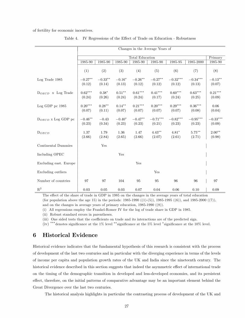
of fertility for economic incentives.

Table 4. IV Regressions of the E¤ect of Trade on Education - Robustness

Changes in the Average Years of

Total Education Primary1985-90 1985-90 1985-90 1985-90 1985-90 1985-95 1985-2000 1985-90

(1) (2) (3) (4) (5) (6) (7) (8)

Log Trade 1985 �0:27�� �0:33�� �0:16� �0:26�� �0:27�� �0:32��� �0:34��� �0:13��(0:12) (0:14) (0:13) (0:12) (0:12) (0:12) (0:13) (0:07)

DOECD x Log Trade 0:62��� 0:38� 0:51�� 0:61��� 0:41��� 0:60��� 0:63��� 0:21���

(0:24) (0:26) (0:24) (0:24) (0:17) (0:24) (0:25) (0:09)

Log GDP pc 1985 0:20��� 0:28�� 0:14�� 0:21��� 0:20��� 0:29��� 0:36��� 0:06(0:07) (0:11) (0:07) (0:07) (0:07) (0:07) (0:08) (0:04)

DOECD x Log GDP pc �0:46�� �0:43 �0:40� �0:47�� �0:71��� �0:82��� �0:95��� �0:33���(0:23) (0:34) (0:23) (0:23) (0:21) (0:23) (0:23) (0:09)

DOECD 1:37 1:79 1:36 1:47 4:43�� 4:81� 5:75�� 2:00��

(2:66) (2:84) (2:65) (2:66) (2:07) (2:61) (2:71) (0:98)

Continental Dummies Yes

Including OPEC Yes

Excluding east. Europe Yes

Excluding outliers Yes

Number of countries 97 97 104 95 95 96 96 97

R2 0:03 0:05 0:03 0:07 0:04 0:06 0:10 0:09

The e¤ect of the share of trade in GDP in 1985 on the changes in the average years of total education(for population above the age 15) in the periods: 1985-1990 ((1)-(5)), 1985-1995 ((6)), and 1985-2000 ((7)),and on the changes in average years of primary education, 1985-1990 ((8)).(i) All regressions employ the Frankel-Romer IV for the log of trade share in GDP in 1985.(ii) Robust standard errors in parentheses.(iii) One sided tests that the coe¢ cients on trade and its interactions are of the predicted sign.(iv) ���denotes signi�cance at the 1% level ��signi�cance at the 5% level �signi�cance at the 10% level.

6 Historical Evidence

Historical evidence indicates that the fundamental hypothesis of this research is consistent with the process

of development of the last two centuries and in particular with the diverging experience in terms of the levels

of income per capita and population growth rates of the UK and India since the nineteenth century. The

historical evidence described in this section suggests that indeed the asymmetric e¤ect of international trade

on the timing of the demographic transition in developed and less-developed economies, and its persistent

e¤ect, therefore, on the initial patterns of comparative advantage may be an important element behind the

Great Divergence over the last two centuries.

The historical analysis highlights in particular the contrasting process of development of the UK and

27

India over the last two centuries. The evidence demonstrates that during the nineteenth century the UK

traded manufactured goods for primary products with India.38 Consistent with the proposed hypothesis,

industrialization in India regressed over this century whereas industrialization in the UK accelerated. The

process of industrialization in the UK led to a signi�cant increase in the demand for skilled labor in the

second phase of the industrial revolution, triggering a demographic transition and a transition to a state

of sustained economic growth. In India, in contrast, the lack of demand for skilled labor delayed the

demographic transition and the process of development. Thus, while the gains from trade were utilized

in the UK primarily towards an increase in output per capita, in India they were more biased towards an

increase in the size of the population.39

6.1 North-South Trade and Industrialization

Consistent with the main hypothesis of this research, during the 19th century, North-South trade, as well as

North-North trade, expanded signi�cantly due to a rapid industrialization in Northwest Europe as well as to

the reduction of trade barriers and transportation costs and the bene�ts of the gold standard. The ratio of

world trade to output was about 2% in 1800, but then it rose to 10% in 1870, to 17% in 1900 and 21% in 1913

(Estavadeordal, Frantz and Taylor, 2002). While much of this trade occurred between industrial economies

a signi�cant proportion was between industrial and non-industrial economies. As shown in Table 5, before

1900 nearly 50% of manufactured exports were to non-European and non-North American economies and

by the end of 19th Century a clear pattern of specialization had emerged. The UK and Northwest Europe

were net importers of primary products and net exporters of manufactured goods, whereas the exports of

Asia, Oceania, Latin America and Africa were overwhelmingly composed of primary products. (Findlay and

O�Rourke, 2001).

Atlantic trade as well as trade with Asia, in an era of colonialism, had major e¤ects on European

growth starting in the late 16th century (Acemoglu et al., 2005). Furthermore, later expansion of inter-

national trade bene�ted and contributed further to the process of industrialization in the UK and Europe

(Mokyr, 1985; Crafts and Thomas, 1986; O�Rourke and Williamson, 1999). For the UK, the proportion of

foreign trade to national income grew from about 10% in the 1780�s to about 26% in the period 1837-45,

and 51% in the period 1909-13 (Kuznets, 1967). Other European economies experienced a similar pattern

as well. The proportion of foreign trade to national income on the eve of World War I was 54% in France,

38% in Germany , 34% in Italy, and 40% in Sweden (Kuznets, 1967). Furthermore, exports were critical for

the viability of some industries, especially the cotton industry, where 70% of the UK output was exported in

the 1870�s (Mokyr, 1989). Thus while technological advances could have spawned the industrial revolution

without an expansion of international trade, the growth in exports increased the pace of industrialization

and the growth rate of output per capita. Moreover, Pomeranz (2000), provides historical evidence for the

38The theory is compatible with the case in which the patterns of specialization are not determined by market forces but ratherby the interaction between colonial forces and international trade. Colonialism reinforced the adverse e¤ect of internationaltrade on the process of industrialization of less developed economies, depressing the demand for human capital and enhancingthe incentive to convert the gains from trade into population growth rather than into an increase in output per capita.39Consistent with the viewpoint that trade has not been uniformly bene�cial across time and regions, recent research has

indicated that the relationship between openness and growth changed in the last century. For example Clemens and Williamson(2004) and Vamvakadis (2002) �nd a negative relationship between openness and growth for the period 1870-1913 and anegative relationship for the period 1970-1998.

28

vital role of trade in the �take o¤�of the European economies. He argues that technological and development

di¤erences between Europe and Asia were minor around 1750, but the discovery of the New World enabled

Europe, via Atlantic trade, to overcome �land constraints�and to take-o¤ technologically.40

Non-industrialized economies were an important market for the export of the industrial economies,

as exhibited in Table 5. Trade with Asia was especially signi�cant for Britain. According to Bairoch (1974)

trade with Asia constituted over 20% of UK total exports throughout the nineteenth century. In contrast,

trade with Asia was only 5% or less of French, German or Italian exports. UK imports from Asia were

also much more important for the UK than for Europe. Bairoch estimates that 23% of UK imports were

originated in Asian countries in 1860 as compared with 12% for continental Europe.

Table 5. Regional Shares of World Trade in Manufactures

1876-1880 1896-1900 1913Exports Imports Exports Imports Exports Imports

U.K. and Ireland 37.8% 9.1% 31.5% 10.4% 25.3% 8.2%Northwest Europe 47.1% 18.1% 45.8% 20.3% 47.9% 24.4%Other Europe 9.2% 13.3% 10.3% 12.2% 8.3% 15.4%U.S. and Canada 4.4% 7.7% 7.4% 9.6% 10.6% 12.1%Rest of the World 1.5% 51.8% 5.0% 47.5% 7.9% 39.9%Source:Yates (1959).

For India, however, international trade played the reverse role. As Chaudhuri (1983) describes, 1813-

1850 was a period of a rapid expansion in the volume of exports and imports which gradually transformed

India from being an exporter of manufactured products �largely textiles �into a supplier of primary com-

modities. Trade with the UK was fundamental in this process, as Table 6 demonstrates, with the UK

supplying over two thirds of its imports for most of the nineteenth century and being the market for over a

third of its exports. Bairoch�s (1974, 1982) analysis of international levels of industrialization and interna-

tional trade supports the viewpoint that international trade was associated with a decrease in the per capita

level of industrialization in India.

Table 6. Share of the Value of British Trade in Total Value of Indian Trade

1828-9 1839-40 1850-1 1860-1 1880-1 1900-1 1920-1 1940-1

Exports 48.2% 57.1% 44.6% 43.1% 41.6% 29.8% 22.1% 34.7%

Imports 65.0% 75.7% 72.1% 84.8% 82.9% 65.6% 60.9% 22.9%

Source: Chaudhuri (1983).

As Table 7 suggests, the rapid industrialization in the UK in the nineteenth century was associated

with a decline in the per capita level of industrialization in India. Furthermore, Bairoch (1974) found that

industries that employed new technologies made up between 60 and 70 percent of the UK manufacturing

40Clark and Feenstra (2001) establish that most of the Great Divergence occurred in the last two centuries and it is originatedby di¤erences in labor e¢ ciency across countries. Moreover, they argue that international trade patterns re�ected thesedi¤erences in labor e¢ ciency.

29

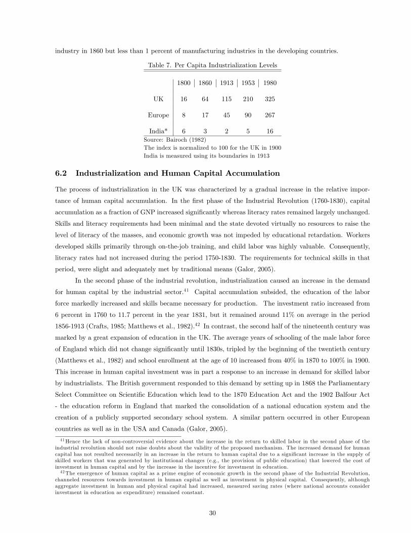
industry in 1860 but less than 1 percent of manufacturing industries in the developing countries.

Table 7. Per Capita Industrialization Levels

1800 1860 1913 1953 1980

UK 16 64 115 210 325

Europe 8 17 45 90 267

India* 6 3 2 5 16Source: Bairoch (1982)The index is normalized to 100 for the UK in 1900India is measured using its boundaries in 1913

6.2 Industrialization and Human Capital Accumulation

The process of industrialization in the UK was characterized by a gradual increase in the relative impor-

tance of human capital accumulation. In the �rst phase of the Industrial Revolution (1760-1830), capital

accumulation as a fraction of GNP increased signi�cantly whereas literacy rates remained largely unchanged.

Skills and literacy requirements had been minimal and the state devoted virtually no resources to raise the

level of literacy of the masses, and economic growth was not impeded by educational retardation. Workers

developed skills primarily through on-the-job training, and child labor was highly valuable. Consequently,

literacy rates had not increased during the period 1750-1830. The requirements for technical skills in that

period, were slight and adequately met by traditional means (Galor, 2005).

In the second phase of the industrial revolution, industrialization caused an increase in the demand

for human capital by the industrial sector.41 Capital accumulation subsided, the education of the labor

force markedly increased and skills became necessary for production. The investment ratio increased from

6 percent in 1760 to 11.7 percent in the year 1831, but it remained around 11% on average in the period

1856-1913 (Crafts, 1985; Matthews et al., 1982).42 In contrast, the second half of the nineteenth century was

marked by a great expansion of education in the UK. The average years of schooling of the male labor force

of England which did not change signi�cantly until 1830s, tripled by the beginning of the twentieth century

(Matthews et al., 1982) and school enrollment at the age of 10 increased from 40% in 1870 to 100% in 1900.

This increase in human capital investment was in part a response to an increase in demand for skilled labor

by industrialists. The British government responded to this demand by setting up in 1868 the Parliamentary

Select Committee on Scienti�c Education which lead to the 1870 Education Act and the 1902 Balfour Act

- the education reform in England that marked the consolidation of a national education system and the

creation of a publicly supported secondary school system. A similar pattern occurred in other European

countries as well as in the USA and Canada (Galor, 2005).

41Hence the lack of non-controversial evidence about the increase in the return to skilled labor in the second phase of theindustrial revolution should not raise doubts about the validity of the proposed mechanism. The increased demand for humancapital has not resulted necessarily in an increase in the return to human capital due to a signi�cant increase in the supply ofskilled workers that was generated by institutional changes (e.g., the provision of public education) that lowered the cost ofinvestment in human capital and by the increase in the incentive for investment in education.42The emergence of human capital as a prime engine of economic growth in the second phase of the Industrial Revolution,

channeled resources towards investment in human capital as well as investment in physical capital. Consequently, althoughaggregate investment in human and physical capital had increased, measured saving rates (where national accounts considerinvestment in education as expenditure) remained constant.

30

Education was not expanded to a similar degree in India in the 19th Century. As noted by Basu

(1974), during the nineteenth century the state of education in India was characterized by a relatively large

university sector, aimed at producing skilled bureaucrats rather than industrialists, alongside widespread

illiteracy of the masses. The literacy rate was very low, (e.g., 10% in Bengal in 1917-8) but nevertheless,

attempts to expand primary education in the twentieth century were hampered by poor attendance and high

drop out rates, which may suggest that the e¤ective rate of return to education was relatively low. The

lack of broad based education in India can also be seen using the data of Barro and Lee (2000). Despite an

expansion of education throughout the twentieth century Barro and Lee report that in 1960 72.2 percent of

Indians aged 15 and above had �no schooling�compared with 2 percent in the UK.

6.3 Industrialization, Population Growth and the Demographic Transition

For the major part of human existence economies appear to have been in a state of Malthusian stagnation.

Diminishing returns to labor along with a positive e¤ect of the standard of living on the growth rate of

population provided a self equilibrating role for the size of the population in a stationary economic environ-

ment. Changes in the technological environment or in the availability of land led to larger but not richer

population. The growth rate of output per capita had been negligible over time and the standard of living

had not di¤ered greatly across countries.

The emergence from Malthusian stagnation in Europe as a whole was initially very slow, (Maddison,

2001). During this slow transition, the Malthusian mechanism linking higher income to higher population

growth continued to function, but the reduction in resources per capita caused by higher population was

counteracted by technological progress, which allowed per capita income to keep rising. The average growth

of output per capita over the period 1820-1870 rose to an annual rate of 1.0 percent along with an impressive

increase in education. During this time interval, fertility rates increased in most of Western Europe until the

second half of the nineteenth century. Furthermore, the acceleration in technological progress increased the

return to human capital and ultimately triggered a demographic transition in which fertility rates declined

rapidly, paving the way to an era of sustained economic growth . The level of resources invested in each

child increased and population growth fell, bringing about a sustained average annual increase in income per

capita of about two percent over the period 1929-1990 (Galor, 2005).

The evolution of population in the UK and India was characterized by these three distinct phases

as well. In the Malthusian phase population increased but income per capita remained roughly constant,

in the early take-o¤ the growth of income per capita and population increased, and in the modern stage a

demographic transition took place and the rate of population growth falls while income per capita rises. In

the UK, population growth increased rapidly during the industrial revolution before declining sharply in the

twentieth century. In contrast India has not until recently experienced a rapid increase in industrialization

and has seen population growth increase with income in a Malthusian manner. This delay in the demographic

transition in India lead, according to the proposed theory, to the divergence between UK and India.

31

7 Concluding Remarks

This research suggests that the transformation in the distribution of income and population across the globe

that accompanied the take-o¤ from an epoch of stagnation to sustained economic growth is partly associated

with the contrasting e¤ects of international trade on the timing of the demographic transition in industrial

and non-industrial countries. In industrial economies international trade has enhanced the specialization

in the production of skilled intensive goods and stimulated technological progress. The rise in the demand

for skilled labor has induced an investment in the quality of the population, expediting the demographic

transition, stimulating technological progress and further enhancing the comparative advantage of these

industrial economies in the production of skilled intensive goods. In non-industrial economies, in contrast,

the specialization in the production of unskilled intensive goods that has been triggered by international

trade has reduced the demand for skilled labor, providing limited incentives to invest in population quality.

The demographic transition has been therefore delayed, increasing further the abundance of unskilled labor

in these economies and enhancing their comparative disadvantage in the production of skilled intensive

goods. International trade has therefore widened the gap between the technological level as well as the

skill abundance of industrial and non-industrial economies, enhancing the initial patterns of comparative

advantage and generating sustained di¤erences in income per capita across countries.

The asymmetric e¤ect of international trade on the timing of the demographic transition in developed

and less-developed economies, and its persistent e¤ect, therefore, on the initial patterns of comparative ad-

vantage, may suggest that the rapid transition of the currently developed economies into a state of sustained

economic growth is associated with the slow transition of less developed economies into a state of sustained

economic growth.

The analysis abstracts from several factors that are relevant for the assessment of the e¤ects of inter-

national trade on population growth and the process of development in less developed economies. Cultural

and institutional di¤erences between countries in the determination of population growth, in the provision

of public education, and in the process of technological change would be re�ected in the demographic char-

acteristics and in the patterns of comparative advantage. Moreover, the adverse e¤ect of international trade

on industrialization and thus on the timing of the demographic transition could have been mitigated by the

positive e¤ect of trade on technological di¤usion across countries. Nevertheless, labor productivity greatly

di¤ers across countries and even among industries in which technologies are very similar. Moreover, since

the rate of technological di¤usion depends upon the appropriateness of factor endowments in the receiving

country, the adverse e¤ect of trade on the factor endowment of less developed economies would slow down

the rate of technological di¤usion.43

In contrast to the existing literature on the dynamics of comparative advantage, the focus on the inter-

action between population growth and comparative advantage and the persistent e¤ect that this interaction

may have on the distribution of population and income in the world economy generates an important new

43The e¤ect of trade on technological di¤usion is discussed by Findlay (1996). The imperfections in this process are illustratedfor instance by Clark (1987) who shows that despite the fact that in 1910 textile machinery was uniform around the world,labor productivity was ten times higher in advanced countries than in the less developed ones. This imperfection may be relatedto the e¤ect of factor endowments on the adoption of technologies (Basu and Weil, 1998); Zeira, 1998; Acemoglu and Zilibotti,2001).

32

insight regarding the distribution of the gains from trade. The theory suggests that even if trade between

developed and less developed economies equalizes output growth in the trading countries, income per capita

of developed and less developed economies will diverge, since in developed economies the growth of total

output will be generated primarily by an increase in output per capita, whereas in less developed economies

the contribution of population growth to the growth of total output will be more signi�cant.

In accordance with the theory, cross country regression analysis supports the hypothesis that inter-

national trade generates opposing e¤ects on fertility rates and education in developed and less developed

economies. It demonstrates that international trade has a positive e¤ect on fertility and a negative e¤ect

on human capital formation in non-OECD economies, whereas in OECD economies, trade triggers a decline

in fertility and an increase in human capital accumulation. Thus, international trade accentuates the initial

patterns of comparative advantage and is likely to a¤ect di¤erently the growth trajectory of population,

human capital, and income per capita of developed and less developed economies.

33

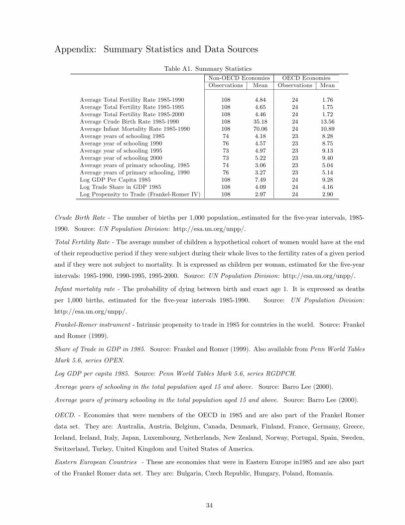
Appendix: Summary Statistics and Data Sources

Table A1. Summary StatisticsNon-OECD Economies OECD EconomiesObservations Mean Observations Mean

Average Total Fertility Rate 1985-1990 108 4:84 24 1:76Average Total Fertility Rate 1985-1995 108 4:65 24 1:75Average Total Fertility Rate 1985-2000 108 4:46 24 1:72Average Crude Birth Rate 1985-1990 108 35:18 24 13:56Average Infant Mortality Rate 1985-1990 108 70:06 24 10:89Average years of schooling 1985 74 4:18 23 8:28Average year of schooling 1990 76 4:57 23 8:75Average year of schooling 1995 73 4:97 23 9:13Average year of schooling 2000 73 5:22 23 9:40Average years of primary schooling, 1985 74 3:06 23 5:04Average years of primary schooling, 1990 76 3:27 23 5:14Log GDP Per Capita 1985 108 7:49 24 9:28Log Trade Share in GDP 1985 108 4:09 24 4:16Log Propensity to Trade (Frankel-Romer IV) 108 2:97 24 2:90

Crude Birth Rate - The number of births per 1,000 population,.estimated for the �ve-year intervals, 1985-

1990. Source: UN Population Division: http://esa.un.org/unpp/.

Total Fertility Rate - The average number of children a hypothetical cohort of women would have at the end

of their reproductive period if they were subject during their whole lives to the fertility rates of a given period

and if they were not subject to mortality. It is expressed as children per woman, estimated for the �ve-year

intervals: 1985-1990, 1990-1995, 1995-2000. Source: UN Population Division: http://esa.un.org/unpp/.

Infant mortality rate - The probability of dying between birth and exact age 1. It is expressed as deaths

per 1,000 births, estimated for the �ve-year intervals 1985-1990. Source: UN Population Division:

http://esa.un.org/unpp/.

Frankel-Romer instrument - Intrinsic propensity to trade in 1985 for countries in the world. Source: Frankel

and Romer (1999).

Share of Trade in GDP in 1985. Source: Frankel and Romer (1999). Also available from Penn World Tables

Mark 5.6, series OPEN.

Log GDP per capita 1985. Source: Penn World Tables Mark 5.6, series RGDPCH.

Average years of schooling in the total population aged 15 and above. Source: Barro Lee (2000).

Average years of primary schooling in the total population aged 15 and above. Source: Barro Lee (2000).

OECD. - Economies that were members of the OECD in 1985 and are also part of the Frankel Romer

data set. They are: Australia, Austria, Belgium, Canada, Denmark, Finland, France, Germany, Greece,

Iceland, Ireland, Italy, Japan, Luxembourg, Netherlands, New Zealand, Norway, Portugal, Spain, Sweden,

Switzerland, Turkey, United Kingdom and United States of America.

Eastern European Countries - These are economies that were in Eastern Europe in1985 and are also part

of the Frankel Romer data set. They are: Bulgaria, Czech Republic, Hungary, Poland, Romania.

34

OPEC - . Economies that were members of OPEC in 1985 and are also part of the Frankel Romer data set.

They are: Algeria, Ecuador, Gabon, Indonesia, Iran (Islamic Republic of), Iraq, Kuwait, Nigeria, Qatar,

Saudi Arabia, United Arab Emirates, Venezuela.

Appendix B

Lemma A1 In the Malthusian stage, if technology is stationary, there exists a unique locally stable steadystate level of population if (i) (1����)=�u > 1; (ii) > [(1����)�(1��)�u]=[(1����)+(1��)�u];and (iii) N0 < (aa0=ec)1=(1� ):

Proof. As follows from Lemma 2 and the individual�s optimization problem, the population dynamic in theMalthusian stage is

Nt+1 =

8<: (1����)(1��)�u [1� (

ecaat)1 N

1�

t ]Nt if �wutpt< ec

(1����)�u Nt if �

wutpt� ec;

Condition (i) of the Lemma ensures that when agents are unconstrained and are rearing only unskilledchildren, the population is rising. Noting the properties of the old agricultural production technology (1),the economy will eventually reach a state where its agents are constrained by the subsistence constraint.The steady state value of N; is

�N = (ecaat)

1 �1 [1� (1� �)�u

(1� �� �) ]

1� :

It is locally stable since as follows from condition (ii):

dNt+1dNt

jNt+1=Nt=(1� �� �)(1� �)�u f1�

1

[1� (1� �)�u

(1� �� �) ]g 2 (�1; 1);

provided, as guaranteed by condition (iii), that the initial level of population is su¢ ciently small so as toassure that the initial average product of labor is not below the subsistence level. �

Proof of Lemma 4.(a) Follows from (A1), (A2) and Lemma 3, noting that g(0) > 0.(b) Lemma A1 shows that under the old technology the unskilled wage, aat (L

a;00 ) �1; tends to the constant

level of ec(1��� �)=[(1��� �)� (1��)�u] � ~wu: However since Aat is rising over time, there exits a timeperiod (ta)� such that, Aat > a

at (L

a;00 ) �1: For (ta)� < t < (tm)� it follows from (13) that the population will

be higher than it would have been in the Malthusian regime. Therefore the shadow Malthusian unskilledwage given by aat ((L

a;0t )�) �1 will be below the level ~wu: (where (La;0t )� is the level of employment in the old

agricultural sector necessary for the old agricultural sector alone to satisfy the total demand for agriculturalproducts at time t): In contrast, Aa will continue to rise. Thus Aat =a

at > ((La;0t )�) �1 still holds. For

(tm)� < t < (tm)��; where (tm)�� is the start of the modern industrial stage, Aat =aat > ((La;0t )�) �1 still

holds since the demand for agricultural goods will be at least as high as it would have been without anynew technologies, and thus the shadow Malthusian unskilled wage will be below the level ~wu.44 Finally, fort > (tm)��, the demand for agricultural goods will be growing at the rate of growth of Aat ; which is a greaterrate than would be occurring under the Malthusian system. Thus again the shadow Malthusian unskilledwage will be below the level ~wu and Aat =a

at > ((L

a;0t )�) �1 still holds. �

Proof of Lemma 5.44For some parameter speci�cations the fall in fertility caused by the introduction of the new industrial technology may

reduce fertility so much and for so long that the population falls below the level it would have attained if the economy hadcontinued on its Malthusian path without the new technologies. If this occurs then we cannot rule out the possibility thataat ((L

a;0t )�) �1 rises above Aa: We regard this as a highly unlikely and very counter factual. Based on McEvedy and Jones�s

(1978), the population of the British Isles grew from 5 million in 1500 to 10 million in 1750. If growth continued at this ratethen the current population of the British Isles would have been 20 million, much below its current actual level of approximately60 million. Hence, the underlying assumption implies that the population at the beginning of the modern industrial stage isgreater than it would have without the existence of the new production technologies.

35

(i) If Y m;Nt+1 = 0; it follows from (14) that wst+1=wut+1 = 0 < �

s=�u and ni;st = 0 for all i: Hence, ht+1 = 0:

(ii) If Y a;Nt+1 > 0 and Y m;Nt+1 > 0 then wst+1=wut+1 = � s=�u and ni;st > 0; for some i; and ht+1 > 0: Let NA

t

and NMt be the number of unskilled individuals employed in the agricultural and the manufacturing sector

in period t, respectively, and let Ht be the number of skilled individuals employed in the manufacturingsector in period t: Hence, NA

t + NMt + Ht = Nt; where Nt is the number of individuals in the working

generation. Let lut and lst be the labor supply of unskilled and skilled individuals, respectively. It follows that

the amount of unskilled labor employed in the agricultural and the manufacturing sectors is La;Nt = lutNAt

and Lm;Nt = lutNMt , respectively, and the amount of skilled labor employed in the manufacturing sector is

Hmt = lstHt, where noting (13), and that A

at = A(�t);

lut =

�[�=(1� �)] + [(1� �� �)=(1� �)]ec=Aat � lu(�t) if �wut =pt < ec

�+ � if �wut =pt � eclst =

�[�=(1� �)] + (�u=� s)[(1� �� �)=(1� �)]ec=Aat � ls(�t) if �wst =pt < ec

�+ � if �wst =pt � ecCase (a): (�wut =pt) < (�w

st =pt) < ec. As follows from (2) and (11), an equilibrium in the agricultural good

market will hold if Ntec = lutNAt A

at . Hence, La;Nt =Nt = lutN

At =Nt = ec=Aat � La(�t): Similarly, using the

equilibrium conditions in the manufacturing sector, Lm;Nt =Nt = lutNMt =Nt � Lm(�t): Finally, as following

from Lemma 1, Hmt =Nt = l

stHt=Nt = (h

m)�lutNMt =Nt � Hm(�t); since lutN

Mt =Nt = L

m(�t): Hence,

ht �Hmt

La;Nt + Lm;Nt +Hmt

=lstHt=Nt

(lutNAt =Nt) + (l

utN

Mt =Nt) + (l

stHt=Nt)

� h(�t):

where h0(�t+1) > 0 since an increase in the level of technology, raises the wage level and leads to an increasein the budget share of manufactured good and hence a rise in the production of the manufactured good andthus an increase in the skill intensity of the labor force.Case (b) ec < (�wut =pt) < (�wst =pt). Equilibrium in the goods sector implies that

YM

ptY A=AMf((hm)�)luNM

ptAAluNA=

f(hm)�NM

wu((hm)�)NA=�

�:

Since lut = lst ; it follows that

h � Hmt

La;Nt + Lm;Nt +Hmt

=lstHt

lutNAt + l

utN

Mt + lstHt

=HtNt:

Thus, noting that Ht = (hm)�NMt and NA

t = [(�=�)f(hm)�NM

t ]=wu((hm)�); it follows that

ht = (hm)�=[((�=�)f(hm)�=(wu((hm)�)) + (hm)� + 1] = eh:

Case (c): (�wut =pt) < ec < (�wst =pt). Following the lines of arguments in case (a) and (b) the result follows.�

Appendix CThis appendix demonstrates that the qualitative results would not alter if the production technology

in the agricultural section remains land-intensive.If the economy is characterized by 3 production technologies: an old agricultural technology, described

in (1) and an old and new industrial technologies described in (3-4), one would need to replace AssumptionA1-A3 with a stronger set of assumptions so as to assure that the technologically advanced economy wouldhave a comparative advantage in the production of industrial goods.

In the three-technology model, the relative price of the agricultural good in terms of the manufacturedgood in period t, is

pt =

8><>:amt

Aat (L

a;Ot ) �1

if Y m;0t > 0

Amt w

u(hmt )

Aat (L

a;Ot ) �1

if Y m;Nt > 0:

36

The productivity parameters are restricted such that in addition to (A1) and (A2)The productivity of the new industrial technology advances more rapidly than that in the agricultural

technology, i.e.,Am(�)

Aa(�)= K� for K > 1: ((A3�))

This implies that the technologically advanced economy will have a comparative advantage in the industrialsector if K is su¢ ciently large.

The advancement in the productivity of the agricultural sector, Aat ;with �t is such that, at some pointet where ht = eh the rate of technological progress rises su¢ ciently high so that the subsistence constraintwill not bind in the future, i.e.,

Aat+1(�t+1)

Aat (�t)> [(1� �� �)=�u](1� ) ((A4�))

where ht � eh. In order to assure that the pattern of trade is consistent with historical patterns will assumethat K is su¢ ciently large for pAt > p

Bt ; when the two economies begin to trade:

Lemma A2 Economy A has a comparative advantage in the industrial good if K is su¢ ciently large.

Proof. Noting (9), pAt > pBt implies that

[AmtAat]A=[

AmtAat]B = K(�At ��

Bt ) > (

[La;Ot ]B

[La;Ot ]A)1�

Thus the inequality will hold for a su¢ ciently large value of K: �

The rest of the results are established straightforwardly subject to (A1), (A2), (A3�) and (A4�).

37

References[1] ACEMOGLU, D., JOHNSON, S. and ROBINSON, J.A. (2005), �Institutions as the Fundamental Cause

of Long-Run Growth�, in Aghion, P. and Durlauf, S. (eds.) Handbook of Economic Growth (Amsterdam:North-Holland).

[2] ACEMOGLU, D. and VENTURA, J. (2002), �The World Income Distribution�, Quarterly Journal ofEconomics, 117, 659-694.

[3] ACEMOGLU, D., and ZILIBOTTI, F. (2001), �Productivity Di¤erences�Quarterly Journal of Eco-nomics, 116, 563-606.

[4] ASHRAF, Q. and GALOR., O. (2007), �Cultural Assimilation, Cultural Di¤usion and the Origin of theWealth of Nations�(CEPR Discussion Papers 6444).

[5] ATKESON, A. and KEHOE, P. (2000), Paths of Development for Early and Late Bloomers in a DynamicHeckscher-Ohlin Model�, (Bank of Minneapolis Sta¤ Report #256).

[6] BALDWIN, R. E., MARTIN, P. and OTTAVIANO, G. I. P. (2001), �Global Income Divergence, Tradeand Industrialization: The Geography of Growth Take-O¤s�, Journal of Economic Growth, 6, 5-37.

[7] BAIROCH, P. (1974), �Geographical Structure and Trade Balance of European Foreign Trade From1800-1970�, Journal of European Economic History 3, 557-608 .

[8] BAIROCH, P. (1982), �International Industrialization Levels from 1750-1980�, Journal of EuropeanEconomic History, 11, 269-333

[9] BARRO, R. J and LEE, J. (2000), �International Data on Educational Attainment: Updates andImplications�(Center for International Development, Harvard University).

[10] BASU, A. (1974), The Growth of Education and Political Development in India 1898-1920. (Oxford:Oxford University Press).

[11] BASU, S. and WEIL, D. N. (1998), �Appropriate Technology and Growth�, Quarterly Journal ofEconomics, 113, 1025-1054.

[12] BECKER, G. S. (1981), A Treatise on the Family (Cambridge MA: Harvard University Press).

[13] CASELLI, F. and COLEMAN, J. W. (2001), �The US structural transformation and regional conver-gence: A reinterpretation�, Journal of Political Economy, 109, 584-616.

[14] CHADHURI, K.N. (1983), Foreign Trade and Balance of Payments (1757-1947) in The CambridgeEconomic History of India D. Kumar (ed.) (Cambridge: Cambridge University Press).

[15] CLARK, G. (1987), �Why Isn�t the Whole World Developed?: Lessons from the Cotton Mills�, Journalof Economic History, 47(1), 141-174.

[16] CLARK, G. and FEENSTRA, R. (2001), �Technology in the Great Divergence�(NBERWorking Paper,8596).

[17] CLEMENS, M.A. and WILLIAMSON., J.G., (2004) �Why Did The Tari¤-Growth Correlation ReverseAfter 1950?�, Journal of Economic Growth, 9, 5-46.

[18] CRAFTS, N.F.R. (1985), British Economic Growth during the Industrial Revolution (Oxford: OxfordUniversity Press).

[19] CRAFTS, N.F.R. and THOMAS, M. (1986) �Comparative Advantage in U.K. Manufacturing Trade,1910-1935�, The Economic Journal, 96, 629-645.

[20] DE LA CROIX, D. and DOEPKE, M. (2003), �Inequality and Growth: Why Di¤erential FertilityMatters�, American Economic Review, 93, 1091-1113.

[21] DOEPKE, M. (2004), �Accounting for Fertility Decline During the Transition to Growth�, Journal ofEconomic Growth, 9, 347-383.

[22] ESTAVADEORDAL, A. and TAYLOR, A. M. (2002), �A Century of Missing Trade�, American Eco-nomic Review, 92, 383-393.

38

[23] ESTAVADEORDAL, A., FRANTZ, B. and TAYLOR, A. M. (2002), �The Rise and Fall of World Trade,1870-1939�, Quarterly Journal of Economics, 118, 359-407.

[24] FINDLAY, R. and KEIRZKOWSKY, H. (1983), �International Trade and Human Capital: A SimpleGeneral Equilibrium Model,�Journal of Political Economy, 91, 957-978.

[25] FINDLAY, R. (1996), �Modeling Global Interdependence: Centers, Peripheries, and Frontiers�, Amer-ican Economic Review, 86, 47-51.

[26] FINDLAY, R. and O�ROURKE, K. H. (2001), �Commodity Market Integration, 1500-2000� in M. D.Bordo, A. M. Taylor and J. G. Williamson (eds.) Globalization in Historical Perspective (Chicago: TheUniversity of Chicago Press).

[27] FRANKEL, J.A., ROMER, D. (1999), �Does Trade Cause Growth", American Economic Review, 89,379-399.

[28] FRANKEL, J.A., ROSE, A. (2002), �An estimate of the E¤ect of Common Currencies on Trade andIncome", Quarterly Journal of Economics, 117, 437-466.

[29] GALOR, O. (2005), �Uni�ed Growth Theory: From Stagnation to Growth,�in Aghion, P. and Durlauf,S. (eds.) Handbook of Economic Growth (Amsterdam: North-Holland).

[30] GALOR, O. and MOAV, O. (2002), �Natural Selection and the Origin of Economic Growth�, QuarterlyJournal of Economics, 117, 1133-1192.

[31] GALOR, O., MOAV, O. and VOLLRATH, D. (2006), �Inequality in Land Ownership, the Emergenceof Human Capital Promoting Institutions and the Great Divergence�(Brown University).

[32] GALOR, O. and MOUNTFORD, A. (2006), �Trade and the Great Divergence: The Family Connection�,American Economic Review, 96, 229-303.

[33] GALOR, O. and WEIL, D. N. (1999), �From Malthusian Stagnation to Modern Growth�, AmericanEconomic Review, 89, 150-154.

[34] GALOR, O. and WEIL, D. N. (2000), �Population, Technology and Growth: From the MalthusianRegime to the Demographic Transition�, American Economic Review, 90, 806-828.

[35] GLAESER, E.L., LA PORTA, R. LOPEZ-DE-SILANES, F. and SHLEIFER, A. (2004), �Do InstitutionsCause Growth?�, Journal of Economic Growth, 9, 271-303.

[36] GREENE, W. H. (1997), Econometric Analysis (New York: Prentice Hall)

[37] GROSSMAN, G. M. and HELPMAN, E. (1991), Innovation and Growth (MIT Press, Cambridge MA).

[38] HAINES, M. R. (2000). �The Population of the United States, 1790-1920�, in Engermann, S. L. and R.E.Gallman (eds), The Cambridge Economic History of the United States, Vol. II, The Long NineteenthCentury, 143-205 (Cambridge: Cambridge University Press).

[39] HARLEY, C. K. (1999), �Reassessing the Industrial Revolution: a Macro View � in J. Mokyr, (ed.),The British Industrial Revolution: an Economic Perspective (Boulder: Westview Press).

[40] HALL, R. E. and JONES, C. I. (1999), �Why Do Some Countries Produce So Much More Output PerWorker Than Others?� Quarterly Journal of Economics, 114, 83-116.

[41] HOWITT, P. and MAYER-FOULKES, D. (2005), �R&D, Implementation and Stagnation: A Schum-peterian Theory of Convergence Clubs�, Journal of Money Credit and Banking, 37, 147-77.

[42] JONES, E. L. (1981), The European Miracle: Environments, Economies and Geopolitics in the Historyof Europe and Asia (Cambridge: Cambridge University Press).

[43] KRUGMAN, P. and VENABLES, A. (1995), �Globalization and the Inequality of Nations�, QuarterlyJournal of Economics, 90, 857-880.

[44] KUZNETS, S. (1967), �Quantitative Aspects of the Economic Growth of Nations : X. Level and Struc-ture of Foreign Trade: Long-Term Trends�, Economic Development and Cultural Change, 15 1-140.

39

[45] LAGERLOF, N.P. (2006), �The Galor-Weil Model Revisited: A Quantitative Exercise�, Review ofEconomic Dynamics, 9, 116-142.

[46] LANDES, D. S. (1998), The Wealth and Poverty of Nations (New York: Norton).

[47] LUCAS, R.. (2002), The Industrial Revolution: Past and Future (Cambridge: Harvard University Press).

[48] MADDISON, A. (2001), The World Economy (Paris : OECD).

[49] MATSUYAMA, K. (1992), �Agricultural Productivity, Comparative Advantage, and EconomicGrowth�, Journal of Economic Theory, 58, 317-334.

[50] MATTHEWS, R. C.O., FEINSTEIN, C. H. and ODLING-SMEE, J. C., (1982), British EconomicGrowth 1856-1973 (Stanford: Stanford University Press).

[51] MCCLOSKEY, D. N., (1981) �The Industrial Revolution, A Survey�in R.C. Floud and D.N. McCloskey,(eds), The Economic History of Britain Since 1700. Vol. 1 (Cambridge: Cambridge University Press).

[52] MCDERMOTT, J. (2002), �Development Dynamics: Economic Integration and the Demographic Tran-sition�, Journal of Economic Growth, 7, 371-410.

[53] MCEVEDY, C. and JONES, R. (1978), Atlas of World Population History (New York: Penguin).

[54] MOKYR, J. (2002), The Gifts of Athena: Historical Origins of the Knowledge Economy (Princeton:Princeton University Press).

[55] MOKYR, J. (1999), �The New Economic History and the Industrial Revolution,� in J. Mokyr, (ed.),The British Industrial Revolution: an Economic Perspective, 1-127 (Boulder: Westview Press).

[56] MOKYR, J. (1985), The Economics of the Industrial Revolution (New Jersey: Rowman and Little�eld).

[57] NORTH, D.C. (1981), Structure and Change in Economic History (New York: Norton).

[58] O�ROURKE, K. H., TAYLOR, A. M. and WILLIAMSON, J. G. (1996), �Factor Price Convergence inthe Late Nineteenth Century�International Economic Review, 37, 499-530.

[59] O�ROURKE, K. H. and WILLIAMSON, J. G. (1999), Globalization and History (Cambridge: MITPress).

[60] O�ROURKE, K. H. and WILLIAMSON, J. G. (2005), � From Malthus to Ohlin: Trade, Industrializationand Distribution Since 1500,�Journal of Economic Growth, 10, 5-34.

[61] POMERANZ, K. (2000), The Great Divergence: China, Europe and the Making of the Modern WorldEconomy (Princeton: Princeton University Press).

[62] RODRIK, D., SUBRAMINIAN, A. and TREBBI, F. (2004), �Institutions Rule: The Primacy of Insti-tutions Over Geography and Integration in Economic Development�, Journal of Economic Growth, 9,131-165.

[63] TREFLER, D. and CHUN ZHU, S. (2005), �The Structure of Factor Content Predictions� (NBERWorking Paper No. W11221).

[64] WOOLDRIDGE J.M. (2002), Econometric Analysis of Cross Section and Panel Data (Cambridge, MA:MIT Press).

[65] WRIGLEY, E. A. (1969), Population and History (New York: McGraw-Hill).

[66] YATES, P. L. (1959), Forty Years of Foreign Trade: A Statistical Handbook With Special Reference toPrimary Products and Underdeveloped Countries (London: Allen & Unwin).

[67] ZEIRA, J. (1998), �Workers, Machines, and Economic Growth�, Quarterly Journal of Economics, 113,1091-1118.

40