Trading in Small World Networks

Gil Shallom∗

May 13, 2010

Abstract

Agents in markets exchange information through social and professional con-tacts. Theory from the world of social networks, biology andphysics suggeststhat such networks should exhibit features of a small world,such as strangersneeding to pass through only a small number of connecting agents to reach eachother, and that each agent is connected to only a few other investors. In a mar-ket where strategic agents are connected through an information exchange net-work exhibiting a small network property highly positive correlated trades, highvolumes and aggressive trading strategies prevail. Contrary to previous modelstrade correlations can also increase with physical distance due to an increase inthe percentage of common information shared. I define the newconcept of in-formational distance to express this real world phenomena not exhibited in othermodels and show the non-monotone relationship between physical distance andinformational distance.

I define a new and more realistic network structure. The informational dis-tance in this structure is a function of two parameters, the number of neighborseach agent has and the number of agents through which a signalpasses withoutstopping. The ability to control for both the distance the signal travels and thenumber of neighbors while maintaining a small world property produces a richset of new predictions regarding trading correlations and volume. Another resultis a linear relationship between the number of units demanded by investors andthe number of investors with whom they share information.

1 Introduction

The effects of information networks on trades in financial markets are not well under-stood and the value of securities are determined in many ways. For example, when oneconsiders choosing a restaurant, there are several sources of information that may beused. One may use one’s own knowledge (private info), look at a published guide suchas the Michelin or the Zagat (public info/central source) or ask for recommendationsfrom friends (network info). Often, the last option is given significant weight in theultimate decision.

∗Haas School of Business, UC Berkeley, Berkeley, CA. email: gilshallom@haas.berkeley.edu.

1

A troubling question when it comes to finance is why wouldn’t we think that thisoccurs in trading? In response to this shortcoming as well as the emergenceof infor-mation network literature in economics (see Jackson [3]), a new stream of research isstarting to appear in finance, such as Fracassi [6] who shows that companies’ levelsof investments and the change over time are more similar as the number of social tiesbetween the companies increases.

This paper describes a market in which participants with social and professionallinks exchange information with each other. Information is either generated internallyby each investor or otherwise privately endowed but then exchanged between investorsfor social reasons and to compare internal analysis with the analyses of other investors.This exchange of information occurs truthfully in expectation of reciprocation in thefuture and the agents then decide on their trades using all the signals that they have.

One can think of fund managers conducting their own internal research regardingcompany valuations and exchanging that information with other fund managers whileusing market noise traders to disguise their actions. Noise is introduced by liquiditytraders who can be individuals or funds doing portfolio balancing, for example, or forother exogenous reasons.

A network structure is created if we look at investors as vertices and the informa-tion links as edges. The network structure we expect is one that exhibits a small worldproperty in a similar fashion to literature from social networks. This paper takes thisidea into the world of multi-period strategic investors who trade with a market makerwhile trying to use liquidity traders to disguise their actions.

The market is comprised of risk-neutral informed traders, who are linkedto eachother in a network, liquidity traders who trade for exogenous reasons and a marketmaker that optimally sets price according to Kyle’s model, where the market makeronly observes the total order flow.

The informed trader’s information set when choosing a trading strategy is com-posed of its own internal signal, the signals of neighbors, and additional investors whoare relatively close to it in the network and the total order flow. Trading takes places inmultiple periods where a trader’s strategy takes into account his own demand, the de-mand of other informed traders with whom his signal was shared, and the price impactof the resulting total demand.

I derive the trading strategies of the informed investors who share information withothers in the network. The market maker’s optimal price function is calculatedalongwith the price impact (Kyle’s lambda [7]).

While previous models involve information and strategic trading, the combinationof a small world property information structure and strategic trading (structure) havenever been jointly analyzed. Previous models involving strategic trading have eitherhad no information network or defined the network structure to be a circle. It is morerealistic to model agents has having multiple social ties than just 2 connections. It isalso more realistic to have the distance between agents in the network to be relativelysmall. As an example, if we consider a fund manager in Dallas and a fund managerin Calcutta, although those are distant agents it is reasonable to assume that the fundmanager in Texas has ties in NYC and that the agent in Calcutta has ties in Delhi that in

2

turn have ties in NYC. Thus although I have conceived of agents who would seem to beas distant as possible in my information network, in my example the physical distancebetween them is only 4-5 connections. Therefore the previous model of acircle inwhich the distance between the most distant agents is half the number of fundsin thenetwork seems very unrealistic. A network structure such as an n-dimensional cubeexhibits these two important features of a large number of neighbors and relativelysmall distance even between the most distant agents in the information network.

Colla & Mele [2], while considering information links and strategic trading, do notexhibit the desired small world property. Therefore they conclude that trade correla-tions must decline as the physical distance between investors in the network increases.A paper which does consider the importance of the small world property is that ofOzoylev & Walden [8], but is in a static setting and studies a different question.

Intuition suggests that it is not the physical distance in the network that mattersbut rather the percentage of common information agents share, i.e. the informationaldistance. I devise an information network structure (n-dimensional cube)that is signif-icantly better in representing features depicted in social network theory from the fieldsof sociology and economics such as the small world property or for our purposes, alarge number of directly linked neighbors and a relatively small distance between themost distant agents.

I construct the network in the model as an n-dimensional cube, where the dimen-sion of the cuben is the first choice variable and an additional choice variable is thedistance to which signals propagate (denoted ask). This structure exhibits the desiredsmall world property as it creates a market withM = 2n investors, each of which hasmerelyn contacts and despite that the distance between the most distant of investors ismerelyn.

A core observation of the model is that investors who are strangers, i.e. do notknow each other through a social or professional link, can have highly positive tradingcorrelation if they have a significant share of common information sources.In fact,strangers can have higher correlations than neighboring investors. Figure 1.2.2 illus-trates this notion and I explain how this phenomenon, which I refer to as informationalproximity vs. physical proximity, comes into play in subsection 1.2.2.

Another important result is that the number of units demanded by investors exhibitsa linear relationship to the number of investors with which information is shared.Thisis consistent with our expectation that an increased sharing of information will resultin higher competition, i.e. higher demands, and as a result faster price convergence.Simply put, the closer the market gets to the full information case, the higher theefficiency of the market, as measured by a reduction in the volatility of the asset.

The following subsections explain the properties of the n-dimensional cubenet-work structure as it is crucial to understand that for the solution of the model. Inaddition I explain the notion of physical vs. informational distance and showthat itexists in my information structure.

3

0 (000) 1 (001)

2 (010) 3 (011)

4 (100) 5 (101)

7 (111)6 (110)

Figure 1: Binary Representation of Cube Vertices

1.1 more references

Feng & Seasholes [4] show correlation of trades for investors geographically close toeach other.

Local bias effects are also important in determining one’s investments and possiblysupports the reason for this to be social ties. Chan, Covrig and Ng [1] provided acomprehensive research of the determinants for local bias. However an alternativeexplanation for the strong local bias is the existence of social ties in the domesticcountry that provide financial information regarding the domestic market.

1.2 Brief introduction to cube combinatorics

1.2.1 Binary arithmetic, combintorical and geometrical properties of a cube

The analysis of the model and computation of the equilibrium requires us to count thenumber of neighbors of each investor. We are familiar with the structure of asquare(2-dimensional cube) or a cube (3-dimensional cube) and can easily count the numberof neighbors in that case, but must switch to a more general accounting method inorder to be able to extend our intuition to the network structure we’re interested in,since it is of a higher dimension.

Each investor is located in a vertex of the cube. If we number our vertices inthestandard decimal notation we do not see any pattern helping us count an investor’sneighbors, but once we switch our numeric representation to a binary base, a wholeworld of patterns suddenly appears.

On the standard cube (illustrated in figure 1.2) we can start from vertex 0,or in 3-digit binary representation 000b. Now going to the right to vertex 1 means changing thefirst digit in the binary representation in order to reach to 001b. Going forward to vertex2 means changing the second digit in the binary representation to reach 010b, and inorder to go up to vertex 4 we need to change the 3rd digit in the binary representationand thus reach at 100b. This phenomena is also true when starting from any othervertex with the only change that going left changes the first digit from 1 to 0, as is thecase for going back or down.

4

We see that we can reach all neighbors of an investor by changing a meresingledigit in the binary representation of its location.

But what happens when we want to reach investors who are at distance2 from us?Well, the answer is easy, if you’re starting at vertex 0 (000b), then change the first digitwhen going to the right to vertex 1 (001b), and change the 3rd digit when going upto vertex 5 (101b). Thus, going to distance 2 requires changing 2 digits out of the 3available in the 3-dimensional cube.

It is easy to confirm that in standard cube vertex 0, (000b) has(

31

)

= 3 neighbors of

distance 1,(

32

)

= 3 neighbors of distance 2 and(

33

)

= 1 neighbors of distance 3.Using this methodology for counting the number of neighbors shows its power

when we move on to the n-dimensional case. In the n-dimensional case, each investorwishing to go to a neighbor of distancek must changek digit in the n-digit repre-sentation of its location. Therefore, in the n-dimensional cube each investor has

(

nk

)

neighbors of distancek.If we’re interested in the number of neighbors of distance≤ k then each investor

has∑k

i=1

(

ni

)

, and we denote this number byC(n, k).In my model I want to calculate the correlations of averages of signals. These aver-

ages are taken on the signals of an investor and its neighbors and therefore correlationin average signals between two investors will depend on the number of neighbors theyhave in common. Thus, I now turn to the calculation of the number of mutual neigh-bors.

Suppose we have two investorsi and j of distanced. If they are extremely farapart (d > 2k), then the neighbors of investori are all different from the neighbors ofinvestor j. If investorsi and j are close to each other (d ≤ k), then the neighbors ofinvestori who are also neighbors of investorj are those who are of distance of onlyk− d away fromi and vice versa for investorj. We can think of it as having onlyk− ddigits that we can change out of then digits in the binary representation. Finally, for amedium distance between investorsi and j (k < l ≤ 2k), we want the neighbors whoare far away enough (at leastd − k), but still not out of the rangek.

Turning the following intuition into a formula, we get the number of mutual neigh-bors up to distancek for 2 vertices of distanced is:

mutualneighbors=

0 if d > 2k∑k

i=d−k

(

di

)

if k < d ≤ 2k∑k−d

i=0

(

di

)

if d ≤ k(1)

or, using our definition ofC(n, k) =∑k

i=0

(

ni

)

we get:

mutualneighbors=

0 if d > 2kC(n, k) −C(n,d − k− 1) if k < d ≤ 2k

C(n, k− d) if d ≤ k(2)

Now I turn to an important feature of the chosen n-dimensional cube structure forour network. Consider the following 2 pairs of investors,i1 & j1 and i2 & j2 and

5

12 3

4

i3

i(n−4)

i(n−3)

i1

i2

i(n−2)

j3

j(n−4)

j(n−3)

j(n−2)

j1

j2

Figure 2: Physical vs. Informational Distance

suppose thati1 & j1 are have a distance ofk < d1 ≤ 2k between them andi2 & j2 havea distance ofd2 < k.

Theorem 1.1. For n ≥ 5∃k < n2, such that there exists d1 and d2 for which C(n, k) −

C(n,d1− k) > C(n, k−d2) or mutualneighbors(i1, j1) > mutualneighbors(i2, j2), i.e.despite the fact that i2 & j2 are closer to each other the more distant pair of investorsi1 & j1 has more mutual neighbors.

Example 1. Let n = 5 andk = 3 and choosed1 = 5 andd2 = 1, then we haveC(5,3)−C(5,5−3−1) = C(5,3)−C(5,1) =

(

52

)

+(

53

)

= 20 compared with the number

of mutual neighbors for the adjacent pair which yieldsC(5,2) =(

50

)

+(

51

)

+(

52

)

= 16.

This feature becomes more pronounced as the dimension of the network increases.

1.2.2 Physical vs. Informational distance on n-dimensional cube

If A and B are any two nodes on the informational network, then lets define:Physical distance between A and B= number of arches in the shortest path between

two nodes A and B. Note that 0≤ physicaldistance≤ n, asn is also the maximumdistance between two investors in our cube (the diameter of the graph).

Informational distance= 1 - (number of common signals shared by the two in-vestors)/(the number of total signals an investor receiver)= 1 - (mutualneighbors)/(C(n,k))Note that 0≤ in f ormationaldistance≤ 1.

Consider the example in figure 1.2.2, investor 2 & 3 are directly connected, i.e.the distance between them is only 1. Investors 3 & 4 are further apart with distance2 between them. Now assume that signals travel a single hop to the nearest neighborand all signals are considered equally important. In this case, investors 2 &3 onlyshare in common only2n of their information set, while investors 3 & 4 sharen−2

n oftheir information set. Thus, information wise we would consider investors 3 & 4to becloser than 1 & 2 despite the fact that the latter pair is closer in physical distance.

6

In Colla & Mele physical distance determines the informational distance of in-vestors.

In this paper I loosen the link between the two while still maintaining an analyticalsolution.

2 Model

We set up the agents and information structure of the model and then solve for theunique Bayesian Nash equilibrium comprised of the informed traders tradingstrategiesand the market makers optimal update rule.

2.1 Construction of the Model

Our investors are arranged in an information network structured as an n-dimensionalcube. Each investor receives an independent signal at his location and exchanges hissignal with neighbors of limited distance from him. Following the information ex-change, each investor decides on his demand for the asset using his knowledge of hisown demand and previous total demand and then submits the order. The market makersets the price, trades with the investors and then the next round of trade begins. Theinvestors use liquidity traders to disguise their actions and the market maker tries tounravel the strategic investors actions from the total liquidity demand that includesboth the strategic investors demand and the liquidity traders demand.

Signals are only exchanged before the first round of trading commences.Assumptions: In order to prove that the model works I need to show the existence

of an equilibrium price and traders strategy.

2.2 Information Structure

The market in my model is consisted ofM = 2n agents, liquidity traders and onemarket maker. The agents are risk neutral profit maximizing and the market makersupplies liquidity and sets the price according to a learning process from theorderflow which is defined in detail in section 2.4.

Each investor receives a signal at his location about the fundamental value f . Lets0 = [s1,0, . . . , sM,0]T be aM = 2n vector of signal in the market. I assume that eachtrader shares his information with traders of physical distance≤ k from him in theinformation network.

Therefore, given the analysis of the previous section (cube combinatorics), theaverage signal available to each trader is composed ofC(n, k) independent signals. Forexample, forn = 7 andk = 2, the signal available to each trader is composed ofS(7,2) =

∑2i=0

(

7i

)

= 1+ 7+ 21= 29 independent signals.

7

2.3 Correlation of Signal and Trades

I have M = 2n investors in the model and assume that investori is endowed with asignal si,0 where the second parameter denotes that this is the signal before the firstround has started (round 0), the entire set of investor signals is combinedinto a vectordenoted bys0 = [s1,0, . . . , sM,0].

I follow Foster and Viswanathan [5] and Colla & Mele [2] and assume that allthesignals are jointly normally distributed with mean zero and variance-covariance matrixequal toΨ0 = E([s1,0, . . . , sM,0]T [s1,0, . . . , sM,0]). The unconditional distribution of thesignals is symmetric in that it is invariant to a permutation of the indices 1, . . . ,M. Forconvenience, I also denote the correlation between initial signals of different investorsby c0 = Cov(si,0, sj,0).

Denoting the fundamental value of the asset byf and the variance (uncertainty) ofthe fundamental value byσ2

f , I continue and assume that the joint distribution of the

vector [f s0]T is given by

[

fs0

]

∼ N

([

00

]

,

[

σ2f c01T

c01T Ψ0

])

, Ψ0 =

Λ0 Ω0 . . . Ω0

Λ0 Ω0. . .

...

Λ0

where we assume thatΨ0 is invertible, which it is, providedΛ0 > −(M − 1)Ω0, arestriction maintained throughout the paper. This restriction ensures that the averageof the average signals, ¯s = 1

M

∑Mi=1 si,0, is a sufficient statistic for the full information

liquidation value,

E( f |s0) = θs (3)

whereθ = c0MΛ0+(M−1)Ω0

(basically cov()/var()).The unconditional variance-covariance matrix of the average signal withΨ =

E([ s1, . . . , s2n]T [ s1, . . . , s2n]).

Ψ0(n, k) =

Λ0(n, k) Ω0(1,n, k) . . . Ω0(M − 1,n, k)Λ0(n, k) Ω0(M − 2,n, k)

. . ....

Λ0(n, k)

and

Λ0(n, k) =Λ0 +

(

∑ki=1

(

ni

))

Ω0∑k

i=0

(

ni

)

+ 1

8

Ω0(l, k) =

0 if l > 2k[

∑ki=l−k (n

i)]

Λ0+[

∑ki=l−k (n

i)][

∑ki=l−k (n

i)−1]

Ω0[

∑ki=1 (n

i)]2 if k < l ≤ 2k

[

∑k−li=0 (n

i)]

Λ0+[

∑k−li=0 (n

i)][

∑k−li=0 (n

i)−1]

Ω0[

∑ki=1 (n

i)]2 if l ≤ k

The correlation between the average signals locatedl positions apart isρ(l, k) =Ω0(l, k)/Λ0(k) varies with the distance.

2.4 Equilibrium Price and Trades

Let (xi,n)nn=1 be the sequence of orders submitted by theith trader over the trading

period.Since traders are risk neutral, trades are chosen to maximize expected profits:

Wi,n = max(xi,t)Nt=n

E

N∑

t=n

( f − pt)xi,n|Fi,n

, n = 1, . . . ,N

The order flow is comprised of the sum of demands submitted by the investors inthe network with the addition of normally distributed demand submitted by liquiditytraders, such that the total demand is as follows:

yt =

M∑

i=1

xi,n + un n = 1, . . . ,N

The market maker commits to offset the order flow according to a semi-strongefficiency rule:

pn = E( f |Fn), t = 1, . . . ,N

whereFn = (yt)nt=1 denotes the market maker’s information set at thenth round,

i.e. the total order flows in all trade rounds up to (and including) the current one.Using this information, the market maker updates his estimate of the average signal

available to any traderi as

tn = E(si |Fn) =

∑Mj=1 E(sj |Ft)

M= E(si |Fn)

which is independent of theith trader’s specific location since the variance-covariancematrixΨ0 is symmetric.

I restrict my attention to an equilibrium in which both the traders’ strategies andthe pricing function are linear with respect to the information structure, that is, (i) eachtrader strategy is linear in his informational advantage relative to the market maker:

9

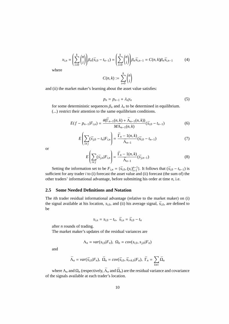
xi,n =

k∑

i=0

(

ni

)

βn(si,0 − tn−1) =

k∑

i=0

(

ni

)

βnsi,n−1 = C(n, k)βnsi,n−1 (4)

where

C(n, k) :=k∑

i=0

(

ni

)

and (ii) the market maker’s learning about the asset value satisfies:

pn = pn−1 + λnyn (5)

for some deterministic sequencesβn andλn to be determined in equilibrium.(...) restrict their attention to the same equilibrium conditions.

E( f − pn−1|Fi,n) =θ(Γn−1(n, k) + Λn−1(n, k))

MΛn−1(n, k)(si,0 − tn−1) (6)

E

∑

i, j

(sj,0 − tn|Fi,n

=Γn − 1(n, k)

Λn−1(si,0 − tn−1) (7)

or

E

∑

i, j

(sj,n|Fi,n

=Γn − 1(n, k)

Λn−1(sj,n−1) (8)

Setting the information set to beFi,n = si,0, (yt)n−1t=1 . It follows that (si,0 − tn−1) is

sufficient for any traderi to (i) forecast the asset value and (ii) forecast (the sum of) theother traders’ informational advantage, before submitting his order at timen, i.e.

2.5 Some Needed Definitions and Notation

The ith trader residual informational advantage (relative to the market maker) on (i)the signal available at his location,si,0, and (ii) his average signal, ¯si,0, are defined tobe

si,n = si,0 − tn, si,n = si,0 − tn

aftern rounds of trading.The market maker’s updates of the residual variances are

Λn = var(si,0|Fn), Ωn = cov(si,0, sj,0|Fn)

and

Λn = var(si,0|Fn), Ωn = cov(si,0, si+k,0|Fn), Γn =∑

k,i

Ωn

whereΛn andΩn (respectively,Λn andΩn) are the residual variance and covarianceof the signals available at each trader’s location.

10

Definition 2.1.σ2

f ,n = Var[E( f |s0|Fn] (9)

2.6 Proofs Needed for Equilibrium

The calculation of the moments conditional on the information set available at roundn have been calculated and proved in the appendix, see lemma A.1. Lemma 4 inappendix stays the same.

The definition ofφn in the equilibrium definition is:

φn =Γn−1(n, k)

(M − 1)Λn−1(n, k)(10)

Lemma 2.2. The price impactλn, i.e. the multiplier of the order flow in the marketmaker update calculation, is given by:

λn =θC(n, k)Mβnσ

2f ,n

(C(n, k)βnM)2σ2f ,n−1 + θ

2σ2u

(11)

σ2f ,n =

1−C(n, k)βnMθC(n, k)Mβnσ

2f ,n

(C(n, k)βnM)2σ2f ,n−1 + θ

2σ2u

σ2f ,n−1 (12)

See proof in the appendix.

2.7 Proof and Calculation of the Unique Bayesian Nash Equilibrium

Theorem 2.3. The necessary and sufficient conditions for a unique Bayesian Nashequilibrium, in which trading strategies and prices are in Equations (4)-(5), are asfollows:

1. The trading strategy coefficientsβn andγn:

βn =θλnσ

2u

C(n, k)Mσ2f ,n

(13)

γn =(1− 2λnµn)[1 − θ−1C(n, k)(M − 1)βnλn]

2λn(1− λnµn)(14)

2.

φn =Γn−1(n, k)

(M − 1)Λn−1(n, k)(15)

3. The full information residual variance satisfies the recursion

σ2f ,n =

1−C(n, k)βnMθC(n, k)Mβnσ

2f ,n

(C(n, k)βnM)2σ2f ,n−1 + θ

2σ2u

σ2f ,n−1 (16)

11

4. Finally, the following inequality must hold:

λn(1− λnµn) > 0 (17)

The following sequence of proofs shows the existence of an equilibrium and cal-culates the equilibrium price and trading strategies.

2.7.1 Step 1: Price Deviation

Using the equilibrium strategies in Equation (4) and (5), the price deviation is

pn − p′n = pn−1 − p′n−1 + λn[∑

j,i

C(n, k)βn(sj,n−1 − s′j,n−1) +C(n, k)βnsi,n−1 − x′i,n] (18)

Plugging equation (B9) from Colla & Mele Lemma 4 p. 37 which states

sj,n−1 − s′j,n−1 =1θ

(p′n−1 − pn−1) (19)

we obtain a recursive equation for the price deviation as follows

pn − p′n = pn−1 − p′n−1 + λn[∑

j,i

C(n, k)βn(1θ

(p′n−1 − pn−1) +C(n, k)βnsi,n−1 − x′i,n]

= (pn−1 − p′n−1)[1 −1θ

C(n, k)(M − 1)βnλn] + λnC(n, k)βnsi,n−1 − λnx′i,n

(20)

2.7.2 Trader’s Behavior Off the Equilibrium Path

x′i,n = C(n, k)βnsi,n−1 + γn(pn−1 − p′n−1) (21)

Wi,n = αns2i,n + ψnsi,n(pn − p′n) + µn(pn − p′n)2 + δn (22)

2.7.3 Step 2: Trader’s Strategies

First I show that equations (21) and (22) from the previous step are mutually consistent.Any traderi faces the following recursive problem:

Wi,n−1 = maxx′i,n

E

f − (p′n−1 + λnx′i,n + λn

∑

j,i

x j,n)

x′i,n +Wi,n

∣

∣

∣

∣

Fi,n

(23)

Given the conjectured value function in Equation (22), the trading strategies inEquation (4) and Equation (21), the optimality condition of the previous problem leadsto the following FOC:

12

0 = E

( f − p′n) − λnx′i,n +∂Wi,n

∂x′i,n

∣

∣

∣

∣

Fi,n

0 = E

( f − pn−1) + (pn−1 − p′n−1) − 2λnx′i,n − λn

∑

j,i

x j,n +∂Wi,n

∂x′i,n

∣

∣

∣

∣

Fi,n

+ E

∂(αns2i,n + ψsi,n(pn − p′n) + µ(pn − p′n)2 + δn)

∂x′i,n

∣

∣

∣

∣

Fi,n

0 = E

( f − pn−1) − λn

∑

j,i

x j,n

∣

∣

∣

∣

Fi,n

+ (pn−1 − p′n−1) − 2λnx′i,n

+ E[

−ψnλnsi,n − 2µn(pn − p′n)(−λn)∣

∣

∣

∣

Fi,n

]

0 = E[

( f − pn−1)∣

∣

∣

∣

Fi,n

]

− λnC(n, k)βnE

∑

j,i

s′j,n

∣

∣

∣

∣

Fi,n

+ (pn−1 − p′n−1) − 2λnx′i,n

− ψnλnE[

si,n]

+ 2λnµnE[

pn − p′n∣

∣

∣

∣

Fi,n

]

0 = E[

( f − pn−1)∣

∣

∣

∣

Fi,n

]

− λnC(n, k)βnE

∑

j,i

(s′j,n − sj,n)∣

∣

∣

∣

Fi,n

+ λnC(n, k)βnE

∑

j,i

sj,n

∣

∣

∣

∣

Fi,n

+ (pn−1 − p′n−1) + λnC(n, k)βnE

∑

j,i

s′j,n

∣

∣

∣

∣

Fi,n

+ (pn−1 − p′n−1) − 2λnx′i,n

− ψnλnE[

si,n]

+ 2λnµnE[

pn − p′n∣

∣

∣

∣

Fi,n

]

(24)

Using Equation (20) the SOC is

−2λn + 2λnµn(−λn) < 0

λn(1− λnµn) > 0 (25)

Using Equation (21) the expected profit in any single auction is

E[( f − pn)x′i,n|Fi,n] = E[( f − pn)C(n, k)βnsi,n−1 + γn(pn−1 − p′n−1)|Fi,n]

(26)

2.7.4 Step 3: Market Maker Updates

3 Results

Theorem 3.1. In the market setting and informational structure described in this pa-per and given an average signal value, there exists a linear relationship between the

13

number of investors with which each investor shares its information and units’ demandfor the asset.

Proof. The number of units of the asset demanded by investori as expressed in equa-tion (4) are:

xi,n = C(n, k)βnsi,n−1 (27)

Suppose that the distance travels a distance ofk + 1 instead ofk, then the numberof neighbors with which investori shares information increases toC(n, k + 1) and theunit demand for the asset increases to:

xi,n = C(n, k+ 1)βnsi,n−1 (28)

That is, the unit demand increases by a multiplier ofC(n,k+1)C(n,k) .

In a similar fashion, an increase in the number of connections each investorhasfrom n to n+ 1 causes a unit demand increase by a multiplier ofC(n+1,k)

C(n,k) .In this sense, the number of units demanded grows linearly with the number of

investors with which investori shares information. ¤

The proof derivations in subsection 2.7 lead me to the following conjecture.

Conjecture 3.2. (yet to be proved): Given any market setting in which all partici-pants are symmetric in the structure of their links of signal exchange, there exists alinear relationship between the number of investors with which each investorsharesits information and the units’ demand for the asset.

Using the proof method used for showing the Bayesian Nash equilibrium in thismodel, I intend to prove this conjecture.

In line with common thinking, as the information is shared with more people, themarket becomes more and more efficient with the extreme case of a full clique graphbeing the complete information case.

Theorem 3.3. Denote the distance between trader i and j in the network by d(i, j),then the trade correlation between investors i and j takes the form:

ρ(xi,n, x j,n) =

0 if d(i, j) > 2kC(n,k)−C(n,d(i, j)−k)

C(n,k) if 2k ≥ d(i, j) ≥ kC(n,k−d(i, j))

C(n,k) if k > 0(29)

Proof.

ρ(xi,n, x j,n) =Cov(xi,n, x j,n)

σ(xi,n)σ(x j,n)

=Cov(C(n, k)βnsi,n−1,C(n, k)βnsj,n−1)

C(n, k)βnσ(si,n−1)C(n, k)βnσ(sj,n−1)

=Cov(si,n−1, sj,n−1)

σ(si,n−1)σ(sj,n−1)

=numo f mutualneighbors

C(n, k)(30)

14

Where the last step relies on the fact that the signals are independent, butdrawn fromthe same distribution. Now by using equation (2) I get the stated outcome. ¤

Corollary 3.4. Strangers can have either lower or higher correlations than investorswho are adjacent to each other in the network.

4 Empirical - To be continued

5 Comparative Statics

I examine different parameter values and the behavior of trade correlations with changesin the parameters. I am considering information exchange between mutual fund man-agers and there are approximately 6,000 funds in the US, therefore excluding smallerfunds with less influence on trade volumes I consider that roughly 211 = 2,048 fundsis a reasonable parameter value for examining implications of the network structure.

Figure 3 and 4 illustrates the changes in trade correlations as agents in the modelgrow further and further apart. The non-monotonicity of the correlationsis evidentfrom the graph and we can see that the trade correlations at first declineas the distancebetween the agents grows but then the correlations increase again as the number ofmutual neighbors grows. This result stems from the properties of the network struc-ture chosen but would result in other network structures exhibiting a largenumber ofneighbors and a small distance between the most distant agents. Figure 4 shows a dropagain in the correlation as the distance increases since the signal propagation distanceis smaller in this case and agents can be far enough so that they do not haveany mu-tual neighbors any more and therefore share no signals. Therefore inthis case, at thelast part, as the distance grows agents share less and less information untiltheir tradecorrelation declines to 0.

In figure 5 I illustrate how the trade correlations change as function of a change inboth the signal propagation distance and the distance between the agents. Examiningthe graph we can see that the signal propagation distance only causes anincrease intrade correlations, while the change in the distance between agents effects the tradecorrelations in a non-monotone fashion as described in the previous paragraph.

6 Conclusions

I have constructed a model with an information structure exhibiting a small worldproperty while maintaining a small number of links for each investor in a mannersimilar to what we come to expect from realistic social networks.

The profit maximization problem of the risk neutral investors and market makeryields a unique Bayesian Nash equilibrium of trading strategies for the investors andmarket impact for the market maker as proved in this paper.

The following predictions are based on the demand, volatility and market impactvalues resulting from the calculation of the equilibrium.

15

0

0.1

0.2

0.3

0.4

0.5

0.6

0.7

0 2 4 6 8 10 12

Tra

de c

orre

latio

n

Physical distance between agents

Trade correlation between agents

Figure 3: The trade correlations of agents as a function of their distance inthe informa-tion network. Parameters n=11,k=7 serve as suggestive dynamics for an informationnetwork of thousands of funds

0

0.05

0.1

0.15

0.2

0.25

0 2 4 6 8 10 12

Tra

de c

orre

latio

n

Physical distance between agents

Trade correlation between agents, k=3

Figure 4: The trade correlations of agents as a function of their distance inthe informa-tion network. Parameters n=11,k=3 serve as suggestive dynamics for an informationnetwork of thousands of funds

16

0

2

4

6

8

10

12

0

2

4

6

8

10

120

0.2

0.4

0.6

0.8

1

Figure 5: The trade correlations as a function of distance and signal propagation dis-tance. Parameters n=11

The model predicts a highly positive trade correlation between most investors(varying with the choice parameterk) due to the relatively small distances betweeninvestors in the social network. Price convergence is also predicted to befast.

An important characteristic of the model is its ability to express the followingnotion: Strangers who share common sources of information can have higher tradecorrelations than investors who happen to be neighbors but don’t haveas much infor-mation in common. The model allows for expressing this phenomenon, i.e. showingthat physical distance is a different notion than informational distance and showing thattrading correlation between informationally close investors can be higher than that ofinvestors which are physically closer to each other.

As preliminary work in linking the model to data, I have constructed an informa-tion network from individual trade data.

The model disentangles the notion of physical and informational distance anddemonstrates the importance of choosing an appropriate network structurefor the shar-ing of signals between investors.

I show that the correlation of trade is related to the informational distance of in-vestors and therefore call for the empirical study of the informational distance of in-vestors in addition to the more apparent physical distance.

Studying only the physical distance of investors in a network would make us un-derestimate the importance of the signal network on the trades we see in the market.It is the distinction which would allow us to guide our empirical studies in a way thatwill allow us to continue to study the impact of social networks on financial markets.

The number of units demanded by investors exhibits a linear relationship with

17

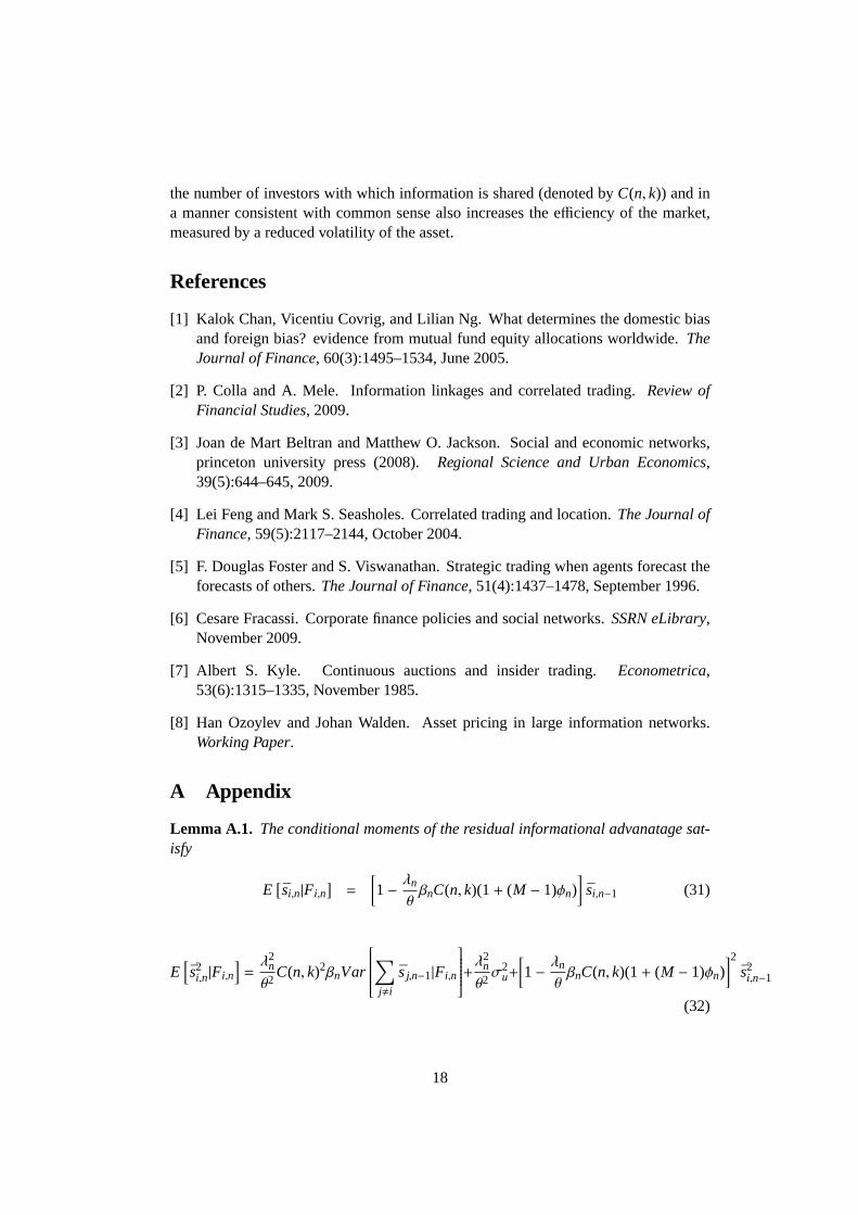
the number of investors with which information is shared (denoted byC(n, k)) and ina manner consistent with common sense also increases the efficiency of the market,measured by a reduced volatility of the asset.

References

[1] Kalok Chan, Vicentiu Covrig, and Lilian Ng. What determines the domestic biasand foreign bias? evidence from mutual fund equity allocations worldwide.TheJournal of Finance, 60(3):1495–1534, June 2005.

[2] P. Colla and A. Mele. Information linkages and correlated trading.Review ofFinancial Studies, 2009.

[3] Joan de Mart Beltran and Matthew O. Jackson. Social and economic networks,princeton university press (2008).Regional Science and Urban Economics,39(5):644–645, 2009.

[4] Lei Feng and Mark S. Seasholes. Correlated trading and location.The Journal ofFinance, 59(5):2117–2144, October 2004.

[5] F. Douglas Foster and S. Viswanathan. Strategic trading when agentsforecast theforecasts of others.The Journal of Finance, 51(4):1437–1478, September 1996.

[6] Cesare Fracassi. Corporate finance policies and social networks. SSRN eLibrary,November 2009.

[7] Albert S. Kyle. Continuous auctions and insider trading.Econometrica,53(6):1315–1335, November 1985.

[8] Han Ozoylev and Johan Walden. Asset pricing in large information networks.Working Paper.

A Appendix

Lemma A.1. The conditional moments of the residual informational advanatage sat-isfy

E[

si,n|Fi,n]

=

[

1−λn

θβnC(n, k)(1+ (M − 1)φn)

]

si,n−1 (31)

E[

s2i,n|Fi,n

]

=λ2

n

θ2C(n, k)2βnVar

∑

j,i

sj,n−1|Fi,n

+λ2

n

θ2σ2

u+

[

1−λn

θβnC(n, k)(1+ (M − 1)φn)

]2

s2i,n−1

(32)

18

Proof.

si,n = si,0 − tn = si,n−1 + tn−1 − tn = si,n−1 − (tn − tn−1)

= si,n−1 − ζnyn = si,n−1 −1θλnyn

= si,n−1 −1θλn

M∑

j=1

x j,n + un

= si,n−1 −1θλn

M∑

j=1

C(n, k)βnsj,n−1

+ un (33)

Taking expectations we get:

E[

si,n|Fi,n]

= E

si,n−1 −1θλn

M∑

j=1

C(n, k)βnsj,n−1

|Fi,n

= si,n−1 −1θβnλnC(n, k)

si,n−1 + E

∑

i, j

si,n−1|Fi,n

= si,n−1 −1θβnλnC(n, k)

si,n−1 +

∑

i, j

Γn−1(k)

Λn−1(k)sj,n−1

by equation (A12) p. 35 Colla& Mele

=

[

1−λn

θβnC(n, k)(1+ (M − 1)φn)

]

si,n−1 (34)

where the last step is by using equation (8) and the definition ofφn.The definition ofφn in the equilibrium definition is:

φn =Γn−1(n, k)

(M − 1)Λn−1(n, k)

Derivation fors2i,n|Fi,n:

E[

s2i,n|Fi,n

]

= Var[

si,n|Fi,n]

+[

E(si,n|Fi,n)]2 (35)

Var[

si,n|Fi,n]

= Var

si,n−1 −1θλn

M∑

j=1

C(n, k)βnsj,n−1 + un

|Fi,n

= Var

λn

θC(n, k)βn

∑

j,i

sj,n−1|Fi,n

+λ2

n

θ2Var[

un|Fi,n]

=λ2

n

θ2C(n, k)2βnVar

∑

j,i

sj,n−1|Fi,n

+λ2

n

θ2σ2

u (36)

19

Thus we get:

E[

s2i,n|Fi,n

]

=λ2

n

θ2C(n, k)2βnVar

∑

j,i

sj,n−1|Fi,n

+λ2

n

θ2σ2

u+

[

1−λn

θβnC(n, k)(1+ (M − 1)φn)

]2

s2i,n−1

(37)¤

Lemma A.2. Let y′n abd t′n be the aggregate order flow and the market maker’s updateof any trader’s average signal, when trader i deviates to(x′i,k)

n−1k=1 during the first n− 1

auctions. The deviation in trader j’s residual advantage,s′j,n = si,0 − t′n, satisfies:

sj,n−1 − s′j,n−1 =1θ

(p′n−1 − pn−1) (38)

Proof. See Lemma 4 in [2]. ¤

Proof of lemma 2.2.we first rewrite the aggregate order flow using equation (4) as:

yn =

M∑

i=1

C(n, k)βnsi,n−1 + un (39)

And since∑M

i=1 si,0 =∑M

i=1 si,0 andtn−1 ∈ Fn−1, then:

cov(si,n−1, yn|Fn−1) = C(n, k)βncov(si,0,

M∑

i=1

si,0|Fn−1)

= C(n, k)βn[Λn + (M − 1)Ωn] = θ−2C(n, k)Mβnσ2f ,n (40)

where the last line follows from Equation (A7) in lemma 2 p. 34 Colla & Mele.Moreover, by equation (A6) in lemma 1 p. 34 Colla & Mele, i.e.pn = θtn and the

fact thatθs− pn−1 =θM

∑Mi=1 si,n−1, the aggregate flow in equation (39) becomes

yn = θ−1C(n, k)βnM(θs− pn−1) + un (41)

so that

Var(yn|Fn−1) = Var(θ−1C(n, k)βnM(θs− pn−1) + un|Fn−1)

= θ−2(C(n, k)βnM)2Var(θs− pn−1)|Fn−1) + σ2u

= θ−2(C(n, k)βnM)2Var(θs|Fn−1) + σ2u

= θ−2(C(n, k)βnM)2σ2f ,n−1 + σ

2u (42)

where the last line follows from Equation (3) and the definition ofσ2f ,n in (9).

Finally, we get

20

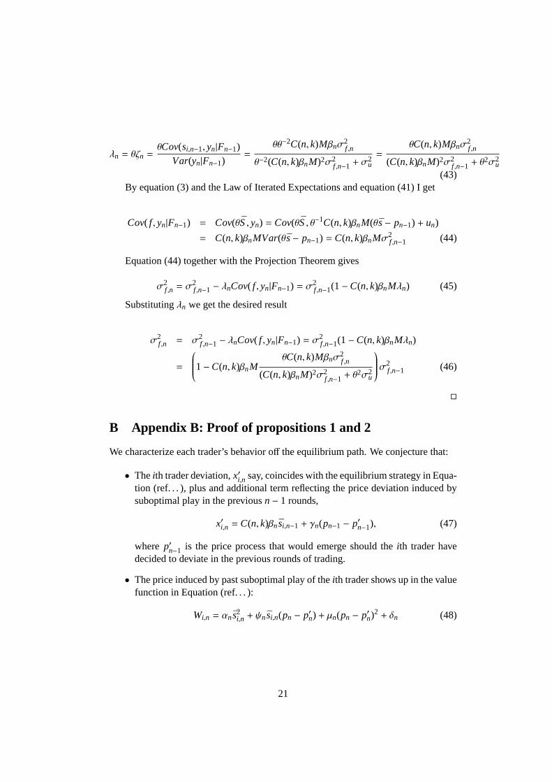
λn = θζn =θCov(si,n−1, yn|Fn−1)

Var(yn|Fn−1)=

θθ−2C(n, k)Mβnσ2f ,n

θ−2(C(n, k)βnM)2σ2f ,n−1 + σ

2u=

θC(n, k)Mβnσ2f ,n

(C(n, k)βnM)2σ2f ,n−1 + θ

2σ2u

(43)By equation (3) and the Law of Iterated Expectations and equation (41) I get

Cov( f , yn|Fn−1) = Cov(θS, yn) = Cov(θS, θ−1C(n, k)βnM(θs− pn−1) + un)

= C(n, k)βnMVar(θs− pn−1) = C(n, k)βnMσ2f ,n−1 (44)

Equation (44) together with the Projection Theorem gives

σ2f ,n = σ

2f ,n−1 − λnCov( f , yn|Fn−1) = σ2

f ,n−1(1−C(n, k)βnMλn) (45)

Substitutingλn we get the desired result

σ2f ,n = σ2

f ,n−1 − λnCov( f , yn|Fn−1) = σ2f ,n−1(1−C(n, k)βnMλn)

=

1−C(n, k)βnMθC(n, k)Mβnσ

2f ,n

(C(n, k)βnM)2σ2f ,n−1 + θ

2σ2u

σ2f ,n−1 (46)

¤

B Appendix B: Proof of propositions 1 and 2

We characterize each trader’s behavior off the equilibrium path. We conjecture that:

• Theith trader deviation,x′i,n say, coincides with the equilibrium strategy in Equa-tion (ref. . . ), plus and additional term reflecting the price deviation induced bysuboptimal play in the previousn− 1 rounds,

x′i,n = C(n, k)βnsi,n−1 + γn(pn−1 − p′n−1), (47)

where p′n−1 is the price process that would emerge should theith trader havedecided to deviate in the previous rounds of trading.

• The price induced by past suboptimal play of theith trader shows up in the valuefunction in Equation (ref. . . ):

Wi,n = αns2i,n + ψnsi,n(pn − p′n) + µn(pn − p′n)2 + δn (48)

21