Traders' Expectations in Asset Markets: …eharuvy/papers/HaruvyLahavNoussair.pdfTraders' Expectations in Asset Markets: ... have shown that changes in the trader population, ... Traders

Traders' Expectations in Asset Markets: Experimental Evidence

By ERNAN HARUVY, YARON LAHAV, AND CHARLES N. NOUSSAIR*

We elicit traders' predictions of future price trajectories in repeated experimental markets for a 15-period-lived asset. We find that individuals' beliefs aboutprices are adaptive, and primarily based on past trends in the current and previous markets in which they have participated. Most traders do not anticipate market downturns the first time they participate in a market, and, when experienced, they typically overestimate the time remaining before market peaks and downturns occur. When prices deviate from fundamental values, belief data are informative to an observer in predicting the direction offuture price movements and the timing of market peaks. (JEL C91, D12, D84, Gil)

The effect of past prices on traders' expectations of future price movements is undisputed. Financial analysts routinely speculate about how particular events and patterns of market activity influence investor expectations, and academic studies have considered how expectations' are formed (see, for example, Roger G. Clarke and Meir Statman 1998, or Kenneth L. Fisher and Statman 2000). A related issue is whether investors' expectations, and their pessimism or optimism about future price trends, are informative about the future direction of the market. Analysts attempt to gauge investor expectations and draw conclusions about the direction of the market from these measures. Though the debate is still ongoing in the academic literature, there are some indications that investor expectations are useful in predicting future price movements

(Wayne Y. Lee, Christine X. Jiang, and Daniel C. Indro 2002; Charles M. C. Lee, Andrei Shleifer, and Richard H. Thaler 1991) and the deviation of market prices from fundamentals (Gregory W. Brown and Michael T. Cliff 2005). The implications of different assumptions of expectation formation on market activity have been extensively investigated (see, for example David P. Brown and Robert H. Jennings 1989; Bruce D. Grundy and Maureen McNichols 1989; Hua He and Jiang Wang 1995; Nicholas Barberis, Shleifer, and Robert Vishny 1998).

While appropriate modeling of expectation formation on the part of traders is crucial to understanding the behavior of asset markets, individuals' beliefs about future prices are typically unobservable to researchers. However, modern methodological techniques in experimental finance and economics allow researchers to overcome this unobservability, and do permit direct measurement of expectations, for some classes of markets. The procedure for doing so is to elicit predictions of future prices from participants or observers of experimental markets, and to provide monetary incentives for accurate forecasts. Several authors have studied expectations in asset markets (Vernon L. Smith, Gerry L. Suchanek, and Arlington W. Williams 1988; Ramon Marimon and Shyam Sunder, 1993; Joep Sonnemans et al. 2004; Cars H. Hommes et al. 2005; Giulio Bottazzi and Maria G. Devetag 2005; Shinichi Hirota and Sunder 2004; Frederic Koessler, Noussair, and Anthony Ziegelmeyer 2005) using this approach.

The focus of this paper is on traders' expectations in repeated experimental markets that

* Haruvy: Department of Marketing, University of Texas- Dallas, 2601 North Floyd Rd., Richardson, TX 75083- 0688 (e-mail: [email protected]); Lahav: Department of Economics, Emory University, 1602 Fishburne Drive, Atlanta, GA 30322-2240 (e-mail: yaron.lahav@gmail. com); Noussair: Department of Economics, Faculty of Eco- nomics and Business Administration, Tilburg University, P.O. Box 90153, 5000 LE Tilburg, the Netherlands (e-mail: [email protected]). We thank seminar participants at the University of Mannheim, Tilburg University, Maastricht University, NHH-Bergen, University of Arizona, Georgia State University, and the University of Melbourne for help- ful comments.

1 Some of these studies examine "trader sentiment," typically stated in terms such as "bullish," "bearish," "pessimistic," or "exuberant." Sentiment is generally only directional, referring to an anticipated increase or decrease in price. In this paper, however, we use the term "expectations" to refer to the point predictions individuals make about future prices.

1901

1902 THE AMERICAN ECONOMIC REVIEW DECEMBER 2007

exhibit price bubbles and crashes, but eventu- ally converge to fundamental values. We consider the role of expectations in generating the bubbles and crashes, and how expectations react to such price patterns. We also study how expectations evolve, respond to, and influence a market as it converges to fundamental pricing. The parametric structure of the asset market we examine was first studied experimentally by Smith, Suchanek, and Williams (1988). We chose this parametric structure in order to facili- tate the interpretation of our results within the existing literature2 and because it reliably pro- duces several market patterns that are of interest to us here. It is well documented that this parametric structure generates bubbles and crashes when market participants are inexperienced with a similar environment. Prices gradually approach fundamentals when the same individuals interact repeatedly in similar markets (Smith, Suchanek, and Williams 1988; Mark B. Van Boening, Williams, and Shawn LaMaster 1993; Martin Dufwenberg, Tobias Lindqvist, and Evan Moore 2005).

In this project, in contrast to the studies cited above, we study individual traders' long-term expectations. While previous studies, beginning with Smith, Suchanek, and Williams (1988),

have elicited predictions of prices for one period into the future, in our design, traders predict the price trajectory over all future periods of the asset's life in a given market, and are permitted to update their predictions after each period of trading. This feature of our design allows us to investigate the relationship between trader expectations of prices in the distant future and price bubbles and crashes. This is essential to understanding the interplay of beliefs and market activity in long-lived asset markets, because in a long-lived asset market, trading decisions may be guided by price expectations for the distant future. Furthermore, unlike previous studies, we also consider expectations of individuals who participate in four consecutive asset markets with an identical structure, and thus are able to track the interdependent relationship between market activity and traders' beliefs until the market fully converges to its fundamental value.

We focus our analysis on the issues raised in the first paragraph. We first study how expectations form and evolve in response to market data, with emphasis on the influence of trends within and between markets and the relationship between experience and expectations. We next examine whether beliefs are accurate predictors of future price movements, including the timing of price peaks. Lastly, we investigate whether observations of traders' price expectations can be useful in forecasting future prices and trends. Section I presents three hypotheses that serve as the basis for the design and analysis of our experiment, Section II describes the experimental design, Section III presents our results, and Section IV provides a conclusion and interpretation of our findings.

I. Hypotheses

Three hypotheses serve as the primary guides for the experimental design and analysis conducted in this paper. The first hypothesis con- cerns the nature of the beliefs that agents hold, and the hypothesis originates from previous experimental work on expectation formation, and the empirical studies listed in the first paragraph of the introduction. While this study is the first to investigate long-term expectations of traders in an experimental market, previous studies of markets in related environments

2 The experiments of Smith, Suchanek, and Williams (1988) have been replicated extensively. See Sunder (1995) for a survey. Subsequent research has shown that bubbles are robust to changes in market trading rules (Van Boening, Williams, and LaMaster 1993). Ronald R. King et al. (1993) have shown that changes in the trader population, the distribution of initial endowments, and margin buying constraints do not reduce bubbles. Bubbles also occur under the addition of a futures market maturing half way through the lifetime of the asset (David P. Porter and Smith 1995), relaxation of cash constraints (Gunduz Caginalp, Porter, and Smith 2000), a fundamental value that is constant over time (Noussair, Stephane Robin, and Bernard Ruffieux 2001), and tournament incentives (Duncan James and R. Mark Isaac 2000). Vivian Lei, Noussair, and Charles R. Plott (2001) have argued that decision errors as well as speculation contribute to bubble formation. Haruvy and Noussair (2006) have shown that prices decrease to levels below fundamental values when sufficiently large short selling capacity is introduced. Noussair and Steven Tucker (2006) have shown that spot market bubbles do not occur if there is a futures market maturing in every future period in operation, along with the spot market for the asset. Experience reduces the incidence and the magnitude of price bubbles (Smith, Suchanek, and Williams 1988; Van Boening, Williams, and LaMaster 1993; Martin Dufwenberg, Lindqvist, and Moore 2005).

VOL. 97 NO. 5 HARUVY ETAL.: TRADERS' EXPECTATIONS INASSETMARKETS 1903

indicate that expectations about the immediate future reflect a continuation of previous market trends. The intuition that expectations are a function of history is also in the spirit of a literature in experimental economics that has modeled play in normal form games under the assumption that individual beliefs are a function of outcomes in the observed past (see for example Vincent P. Crawford 1995; Yin-Wang Cheung and Daniel Friedman 1997; Colin F. Camerer and Teck-Hua Ho 1999; and Drew Fudenberg and David Levine 1998). Thus, we hypothesize that expectations are a function of prior market trends.

In the design that we consider, which is described in detail in Section II, subjects participate in a sequence of identical markets. Therefore, there are two trends that might rea- sonably be expected to be important in the formation of expectations about future prices. The first is the trend of price evolution from one period to the next within the current market. The second is the trend between one period and the next in prior markets. Expectations may reflect a continuation of trends in price changes over the sequence of markets. The hypothesis is stated informally below and given a precise specification in Section III.

HYPOTHESIS 1: Individuals' price expectations are a function of price trends within the current market, as well as in prior markets.

Notice that support of Hypothesis 1 requires that in a market that is in a bubble, such as is often the case for the markets studied here, beliefs do not coincide with fundamental values. However, while Hypothesis 1 indicates that beliefs are backward looking, it does allow, without imply- ing, that expectations are unbiased in predicting actual future prices. The second hypothesis of our study, stated informally below and given a specific testable formulation in Section III, is that individuals have unbiased expectations about future market activity. We consider the validity of the hypothesis with regard to short-term price movements and the timing of market peaks.

HYPOTHESIS 2: Individuals' price expectations are unbiased predictors of future price movements and of the time at which price peaks Occur.

The third hypothesis is motivated by the empirical work described earlier indicating that expectations influence market activity. In other words, the information contained in traders' expectations is useful to an observer trying to predict future price movements. Notice that the hypothesis is not necessarily supported if individuals' price expectations are unbiased, because expectation information may offer no additional predictive power to an observer who already uses the price data and the fundamental value to form predictions. We consider whether an observer with knowledge of trader predictions can predict price patterns better than one could predict using simple rules based on prior trends and fundamental value information. We investigate the issue with respect to predictions of future price movements and the timing of market peaks.

HYPOTHESIS 3: Information on trader expectations provides an observer with additional power to predict price movements and market peaks beyond that from knowing (a) the difference between current price and fundamental value, and (b) the prior price history of the market.

II. Experimental Design and Procedures

The data were gathered in six experimental sessions conducted at Emory University, located in Atlanta, Georgia. All participants were under- graduate students who were inexperienced in asset market experiments. Nine subjects participated in each session (with one session having only eight subjects), and no individual participated in more than one session. Each session lasted approximately three hours, including the first 45 minutes during which the experimenter read the instructions and trained the participants in the use of the market software. Earnings averaged 45 US dollars per subject. In five of six sessions, four markets were organized that operated sequentially. One session consisted of three sequential markets. In each market, participants could trade an asset with a life of 15 periods.

Each of the nine participants possessed an initial endowment of cash and units of the asset at the beginning of period 1 in each of the four markets. Three participants were endowed with three units of the asset and 112 francs (the


experimental currency), three more participants were endowed with two units of the asset and 292 francs, and the remaining three were endowed with one unit of the asset and 472 francs. An individual's initial cash balance and asset inventory at the beginning of period 1 was the same in each market, and the inventory and balances held at the end of period 15 disappeared after the period dividend was paid and total earnings for that market were calculated. Within each market, however, individual inventories of asset and cash balances carried over from one period to the next. That is, the quantities of cash and assets an individual had at the end of period t of market m after the dividend had been paid equaled his quantities of cash and assets at the beginning of period t + 1 of market m. The exchange rate of experimental currency to US dollars was 70 francs of earnings in the markets to one dollar of compensation to the participant. The market was computerized and used call market trading rules implemented with the z-Tree computer program (Urs Fischbacher 2007).

The parameters, including the allocation of individual endowments of shares and cash balances, the number of periods and traders, and the distribution of dividends, were identical to those in design 4 of Smith, Suchanek, and Williams (1988), but with the dividend payments and cash balances equal to one franc in our study for every two US cents in theirs. Specifically, at the end of each period, each unit of the asset paid a dividend of 0, 4, 14, or 30 francs, each with equal probability. The dividend was independently drawn for each period. The distribution of the dividends and the fact that the expected dividend was 12 francs per period were common knowledge among the participants. The participants received a table at the beginning of the experiment describing the expected value of the asset's dividend stream at the beginning of each period. The fundamental value of the asset in any period t equaled the expected dividend in each period, 12 francs, times the number of dividend draws remaining (16 - t draws).

A market for the asset operated each period. The market employed call market rules (as in, for example, Friedman 1993; Van Boening, Williams, and LaMaster 1993; and Timothy N. Cason and Friedman 1997). In a call market, all bids and asks for a period are submitted simultaneously, aggregated into market demand and

supply curves, and the market is cleared at a uniform price for all transactions of that period. The call market design is better suited for the purpose of belief elicitation than the more com- monly used continuous double-auction design. In a double auction market, different units typically trade at different prices within periods. This makes beliefs about prices in future periods more difficult to elicit, since a "period price" is not unambiguously defined. See Sunder (1995) for more detailed discussion of the advantages and disadvantages of call market versus continuous double-auction design.

In each period, each participant had an opportunity to submit one buy order and one sell order to the market. An individual's submitted buy order consisted of only one price and a maximum quantity the individual was will- ing to purchase at that price. Similarly, his sell order consisted of only one price and a maximum quantity the individual offered to sell at that price. Individuals did not observe any other agent's orders for the period when submitting their own orders. After all the participants submitted their decisions, the computer calculated the market price-the lowest equilibrium price in the intersection of the market demand and supply curves constructed from the individual buy and sell orders. Participants who submitted buy orders at prices above the market price made purchases, and those who submitted sell orders at prices below the market price made sales. Any ties for last accepted buy or sell order were broken randomly. Participants were not permitted to sell short or to borrow funds.

Before submitting their orders for each period, the participants were asked to predict the market prices in every future period for the market currently in progress. For example, before period 1, each individual was required to submit 15 predictions, one prediction for each of the prices in periods 1-15 of the current market. Before period 12, each individual submitted four predictions, one each for periods 12, 13, 14, and 15. Individuals typed their predictions into designated fields on their computer screens. Each participant received a payment for accurate predictions, and the closer a prediction was to the actual closing price, the higher the payment that was awarded. Table 1 describes the payment schedule in effect for each prediction any individual submitted. While a quadratic

VOL. 97 NO. 5 HARUVYETAL.: TRADERS' EXPECTATIONS INASSETMARKETS 1905

TABLE 1-PAYMENT SCHEDULE FOR ACCURACY OF

PREDICTIONS: ALL INDIVIDUALS, MARKETS, AND SESSIONS

Earnings to individual Level of accuracy submitting prediction

Within 10 percent of actual price 5 francs Within 25 percent of actual price 2 francs Within 50 percent of actual price 1 franc

scoring rule is often used for belief elicitation (Allen H. Murphy and Robert L. Winkler 1970; Bruno DeFinetti 1965), we chose our incentive scheme in order to keep instructions simple in this relatively complex experiment.

The level of payment reflected a trade-off between being high enough to motivate the participants to submit predictions that were consistent with their true beliefs, and being low enough to prevent trading based on the incentive to receive the payments for accurate prediction. As we note in Section III, the market price patterns are similar to those observed in previous studies in which expectations were not elicited. This indicates that the elicitation of beliefs did not distort market patterns in any qualitative way. The accuracy of each prediction was evalu- ated separately. For example, a participant who predicted the actual market price of period 15 within 10 percent at the beginning of period 10, as well as at the beginning of period 11, received a separate monetary payment for each of the two forecasts.

The information provided to each individual at the end of each period consisted of the market price, the dividend, the number of units of asset he acquired and sold, his current inventory of the asset, the cash he received from sales and spent on purchases, his current cash balance, the income he earned from predictions (sorted by accuracy, 10 percent, 25 percent, and 50 percent), and the cumulative earnings for the session. Prices from all previous periods and markets were displayed in a table on the computer screen at the time subjects submitted their predictions, as well as at the time they submitted their market orders.

III. Results

We first present the overall patterns in market prices, and verify that in our experiment (a) the bubble/crash pattern is observed when traders

are inexperienced, and (b) the magnitude of bubbles decreases with repetition of the market, converging to close to fundamental values in market 4. Therefore, the elicitation of beliefs did not affect the qualitative patterns observed in previous studies of markets with a similar structure. We then present some general patterns in belief statements. We note that individuals fail to predict that a crash will occur in market 1, and that they consistently overestimate the time remaining before the peak price period, the period in which the highest price is observed, in markets 2-4. At the beginning of each of these markets, traders also consistently overestimate the magnitude of the bubbles that will occur in future periods of the current market. This bias, coupled with the fact that bubbles decline in magnitude as the market is repeated, suggests that prices converge toward fundamentals ahead of beliefs.

In Section IIIB, we analyze the determinants of expectations of price patterns in the market in detail, and find that expectations are primarily adaptive. They reflect anticipation of a continuation of previous trends from one period to the next, as well as from one market to the next, supporting Hypothesis 1. Expectations of market peaks are also consistent with a simple model of adaptive dynamics. The existence of adaptive dynamics suggests the mechanism whereby convergence toward fundamental values occurs in this type of asset market. Traders employ profitable strategies given their adaptive expectations, increasing net market demand when they expect prices to rise, while increasing net supply when they believe that a market peak and downturn is approaching. Because this behavior causes market prices to deviate from expectations, Hypothesis 2 is not supported in markets where a bubble occurs. The trading behavior just described reduces the size of bubbles and induces earlier price peaks with repetition of the market, moving the time series of transaction prices closer to fundamentals. After prices and expectations have converged to fundamentals, the data are consistent with Hypothesis 2, and expectations have become accurate predictors of future prices.

We then consider, in Section IIIC, whether an observer of all of the belief data can use the data to improve the accuracy of predictions of future prices and price changes. We find that the belief


Price

500

400

300

200

100

0

Market 1

FV

Session 1 Session 2 Session 3 Session 4

Session 5 Session 6

0 5 10 15

Period

Price

500

400

300

200

100

0

Market 3

FV

Session 1 Session 2 Session 3 Session 4 Session 5 Session 6

0 5 10 15

Period

Price

500

400

300

200

100

0

Market 2

FV

Session 1

Session 2

Session 3 Session 4 Session 5 Session 6

0 5 10 15

Period

Price

500

400

300

200

100

0

Market 4

FV

Session 2 Session 3 Session 4

Session 5 Session 6

0 5 10 15 Period

FIGURE 1. TRANSACTION PRICE IN EACH PERIOD, ALL MARKETS AND SESSIONS

information, when suitably transformed and interpreted to account for traders' biases, can be a very useful tool to predict future price movements and market peaks, supporting Hypothesis 3. Belief information improves predictions of future market activity beyond the predictions obtained from the use of previous price trends and fundamental value information alone.

A. Descriptive Summary of the Data

Figure 1 illustrates the transaction price in each period of each market in each session, along with the fundamental value. Each panel corresponds to one of the markets, and within each panel, each time series represents the activity in one session. The figure conveys the impression that markets populated with inexperienced subjects exhibit bubbles and crashes, and bubbles

become smaller in magnitude as subjects gain more experience.

In market 1, shown in the upper-left panel of the figure, there is a general tendency for bubbles to form. Prices increase over the first ten periods to prices greater than fundamental values in all sessions. Define the peak price period of a market m as the period in which the highest price occurs (if there is a tie, we select the last period satisfying this condition). In market 1, the peak price period averages 12.3. All but one of the markets exhibit a crash, if a crash is defined as a decrease of at least 60 francs (two-thirds of the average value of the fundamental) in price from one period to the next, some time in periods 13-15. While we recognize that crashes are of interest, in the analysis that follows, we will use the peak price period as a measure of the timing of a change in market direction rather than a crash. This is because the peak price period is

VOL. 97 NO. 5 HARUVYETAL.: TRADERS' EXPECTATIONS INASSETMARKETS 1907

Frequency

3

2

1

Market 1

1 2 3 4 5 6 7 8 9 1011 12 131415

Peak price period

Frequency

3

2

1

Market 3

1 2 3 4 5 6 7 8 9 1011 12 13 1415

Peak price period

Frequency

3

2

1

Market 2

1 2 3 4 5 6 7 8 9 1011 12 13 1415

Peak price period

Frequency

3

2

0

Market 4

1 2 3 4 5 6 7 8 9 1011 12 13 1415

Peak price period

FIGURE 2. ACTUAL PEAK PRICE PERIOD IN EACH MARKET, ALL SESSIONS

unambiguously defined, while the definition of a crash is somewhat arbitrary.

In market 2, there is also a tendency for bubbles and crashes to occur, although the bubbles tend to be smaller in magnitude and crashes earlier in occurrence than in market 1. The market price peak occurs on average in period 7 in market 2. The trend toward smaller bubbles and crashes and earlier peak price periods continues during markets 3 and 4. The price peak occurs on average in periods 3.7 and 2.8, in markets 3 and 4, respectively. A histogram of the period in which the price peak occurs is shown in Figure 2. The horizontal axis indicates the market period in which the price peak occurs. The vertical axes show the counts of the number of sessions in which the price peak occurs during each particular period. Each panel corresponds to one of the markets. The figure illustrates the strong tendency for peak price periods to occur earlier

and earlier from one market to the next. This is consistent with convergence to fundamentals, which implies a peak price period of 1.

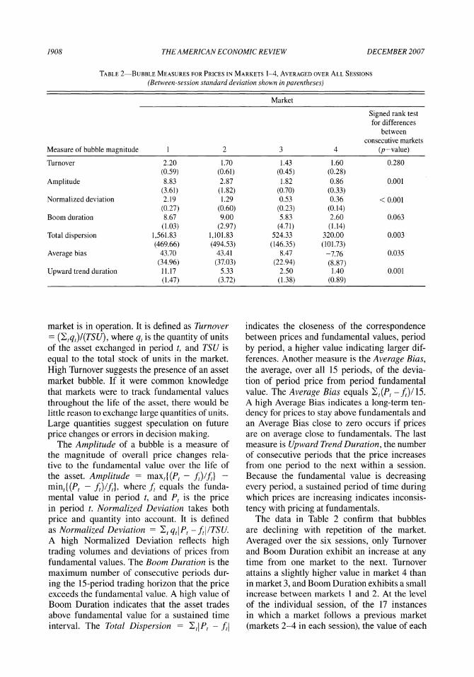
Comparison of the values of several measures of bubbles, which previous authors have introduced to the literature (see Ronald R. King et al. 1993; Van Boening, Williams, and LaMaster 1993; Haruvy and Noussair 2006), confirms the result that bubbles decline with experience. This result is consistent with other studies that have examined the impact of experience (e.g., Van Boening, Williams, and LaMaster 1993; Dufwenberg, Lindqvist, and Moore 2005). The data are shown in Table 2, which indicates the value of each measure in each market, averaged across all of the sessions. A higher value of any of the variables is associated with a bubble of larger magnitude. Turnover is a simple normalized measure of the amount of trading activity over the course of the 15 periods that the


TABLE 2-BUBBLE MEASURES FOR PRICES IN MARKETS 1-4, AVERAGED OVER ALL SESSIONS

(Between-session standard deviation shown in parentheses)

Market

Signed rank test for differences

between consecutive markets

Measure of bubble magnitude 1 2 3 4 (p-value)

Turnover 2.20 1.70 1.43 1.60 0.280 (0.59) (0.61) (0.45) (0.28)

Amplitude 8.83 2.87 1.82 0.86 0.001 (3.61) (1.82) (0.70) (0.33)

Normalized deviation 2.19 1.29 0.53 0.36 < 0.001 (0.27) (0.60) (0.23) (0.14)

Boom duration 8.67 9.00 5.83 2.60 0.063 (1.03) (2.97) (4.71) (1.14)

Total dispersion 1,561.83 1,101.83 524.33 320.00 0.003 (469.66) (494.53) (146.35) (101.73)

Average bias 43.70 43.41 8.47 -7.76 0.035 (34.96) (37.03) (22.94) (8.87)

Upward trend duration 11.17 5.33 2.50 1.40 0.001 (1.47) (3.72) (1.38) (0.89)

market is in operation. It is defined as Turnover = (tq,)/(TSU), where q, is the quantity of units of the asset exchanged in period t, and TSU is equal to the total stock of units in the market. High Turnover suggests the presence of an asset market bubble. If it were common knowledge that markets were to track fundamental values throughout the life of the asset, there would be little reason to exchange large quantities of units. Large quantities suggest speculation on future price changes or errors in decision making.

The Amplitude of a bubble is a measure of the magnitude of overall price changes relative to the fundamental value over the life of the asset. Amplitude = maxt((Pt - ft)/ft} - mintI(Pt - ft)/f,}, where f, equals the fundamental value in period t, and P, is the price in period t. Normalized Deviation takes both price and quantity into account. It is defined as Normalized Deviation = , ql P, - ftI /TSU. A high Normalized Deviation reflects high trading volumes and deviations of prices from fundamental values. The Boom Duration is the maximum number of consecutive periods during the 15-period trading horizon that the price exceeds the fundamental value. A high value of Boom Duration indicates that the asset trades above fundamental value for a sustained time interval. The Total Dispersion = t| P, - f,

indicates the closeness of the correspondence between prices and fundamental values, period by period, a higher value indicating larger differences. Another measure is the Average Bias, the average, over all 15 periods, of the deviation of period price from period fundamental value. The Average Bias equals I,(P, - f,)/15. A high Average Bias indicates a long-term tendency for prices to stay above fundamentals and an Average Bias close to zero occurs if prices are on average close to fundamentals. The last measure is Upward Trend Duration, the number of consecutive periods that the price increases from one period to the next within a session. Because the fundamental value is decreasing every period, a sustained period of time during which prices are increasing indicates inconsistency with pricing at fundamentals.

The data in Table 2 confirm that bubbles are declining with repetition of the market. Averaged over the six sessions, only Turnover and Boom Duration exhibit an increase at any time from one market to the next. Turnover attains a slightly higher value in market 4 than in market 3, and Boom Duration exhibits a small increase between markets 1 and 2. At the level of the individual session, of the 17 instances in which a market follows a previous market (markets 2-4 in each session), the value of each

VOL. 97 NO. 5 HARUVY ETAL.: TRADERS' EXPECTATIONS INASSET MARKETS 1909

Market 1

15 i4

13 12

11 10

9

Period of elicitation

8

7

6

5

4

3

2

1

level

Period forecasted

Price lOO0 200

300

400

5000

Market 3

15 k14

13 !2

S11 lo

9


8

7

6.

5

4

3

2

1 Period forecasted

100- Price level

200

300-

400

500

Market 2

1,5 14

13 '12

11 10

9


8 7

6

5

4

3

2

1

Period forecasted

100

200 Price level

300

400

500

Market 4

15 14

13 12

11 10

9


8 7

8

5

4

3

2

1 Period forecasted

100-

200

Price level

300

400

500

FIGURE 3. AVERAGE PREDICTION FOR EACH PERIOD IN EACH MARKET, SESSION 6

measure is decreasing at least 11 times, with Total Dispersion and Normalized Deviation decreasing in 16 of 17 possible instances. For the pooled data from all sessions, a Wilcoxon signed rank test for differences between consecutive markets (treating any two consecutive markets within a session as a unit of observation for a total of 17 observations) rejects the hypotheses that Total Dispersion, Average Bias, Amplitude, Normalized Deviation, and Upward Trend Duration are not changing from one period to the next, in favor of the hypothesis that they are decreasing. The differences in Turnover and Boom Duration between consecutive markets are not significant at the 5 percent level by the signed rank test.

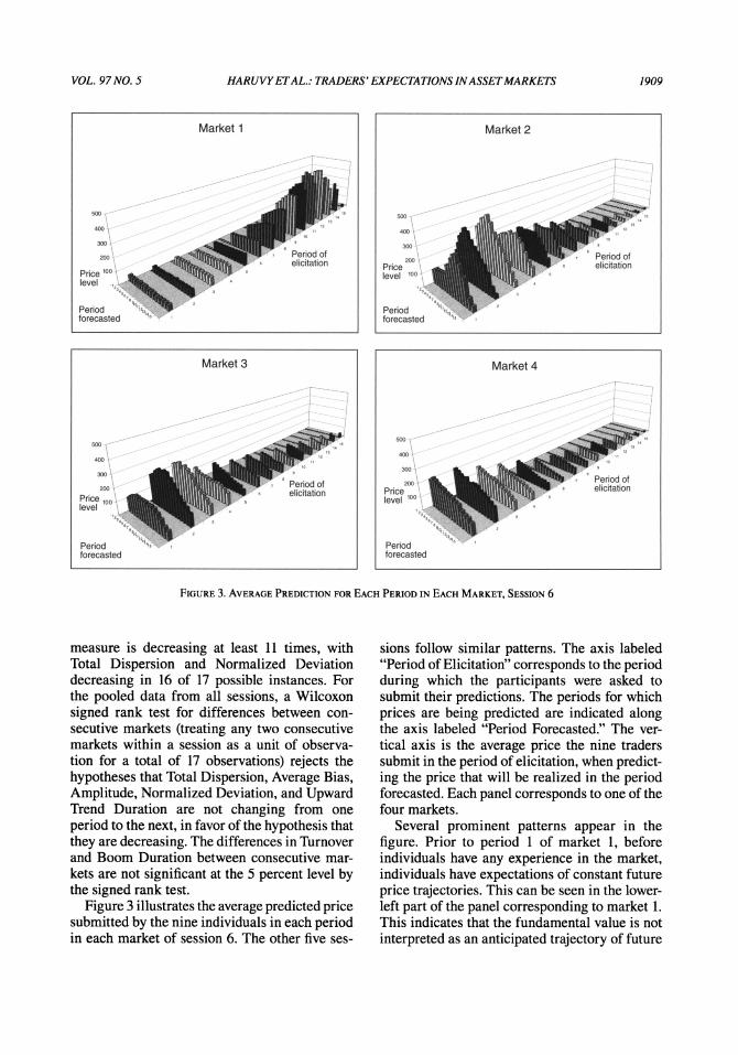
Figure 3 illustrates the average predicted price submitted by the nine individuals in each period in each market of session 6. The other five ses-

sions follow similar patterns. The axis labeled "Period of Elicitation" corresponds to the period during which the participants were asked to submit their predictions. The periods for which prices are being predicted are indicated along the axis labeled "Period Forecasted." The vertical axis is the average price the nine traders submit in the period of elicitation, when predicting the price that will be realized in the period forecasted. Each panel corresponds to one of the four markets.

Several prominent patterns appear in the figure. Prior to period 1 of market 1, before individuals have any experience in the market, individuals have expectations of constant future price trajectories. This can be seen in the lower- left part of the panel corresponding to market 1. This indicates that the fundamental value is not interpreted as an anticipated trajectory of future


prices. This is the case even though the dividend process was prominently emphasized, in the explanation of the environment during the instruction at the beginning of the experiment, and thus these markets can be viewed as "best- case scenarios" for the existence of initial expectations that prices will track fundamentals.

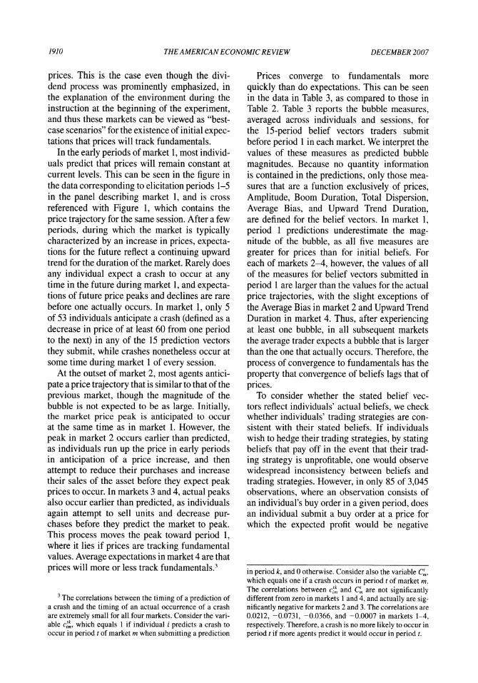
In the early periods of market 1, most individuals predict that prices will remain constant at current levels. This can be seen in the figure in the data corresponding to elicitation periods 1-5 in the panel describing market 1, and is cross referenced with Figure 1, which contains the price trajectory for the same session. After a few periods, during which the market is typically characterized by an increase in prices, expectations for the future reflect a continuing upward trend for the duration of the market. Rarely does any individual expect a crash to occur at any time in the future during market 1, and expectations of future price peaks and declines are rare before one actually occurs. In market 1, only 5 of 53 individuals anticipate a crash (defined as a decrease in price of at least 60 from one period to the next) in any of the 15 prediction vectors they submit, while crashes nonetheless occur at some time during market 1 of every session.

At the outset of market 2, most agents anticipate a price trajectory that is similar to that of the previous market, though the magnitude of the bubble is not expected to be as large. Initially, the market price peak is anticipated to occur at the same time as in market 1. However, the peak in market 2 occurs earlier than predicted, as individuals run up the price in early periods in anticipation of a price increase, and then attempt to reduce their purchases and increase their sales of the asset before they expect peak prices to occur. In markets 3 and 4, actual peaks also occur earlier than predicted, as individuals again attempt to sell units and decrease purchases before they predict the market to peak. This process moves the peak toward period 1, where it lies if prices are tracking fundamental values. Average expectations in market 4 are that prices will more or less track fundamentals.3

Prices converge to fundamentals more quickly than do expectations. This can be seen in the data in Table 3, as compared to those in Table 2. Table 3 reports the bubble measures, averaged across individuals and sessions, for the 15-period belief vectors traders submit before period 1 in each market. We interpret the values of these measures as predicted bubble magnitudes. Because no quantity information is contained in the predictions, only those measures that are a function exclusively of prices, Amplitude, Boom Duration, Total Dispersion, Average Bias, and Upward Trend Duration, are defined for the belief vectors. In market 1, period 1 predictions underestimate the magnitude of the bubble, as all five measures are greater for prices than for initial beliefs. For each of markets 2-4, however, the values of all of the measures for belief vectors submitted in period 1 are larger than the values for the actual price trajectories, with the slight exceptions of the Average Bias in market 2 and Upward Trend Duration in market 4. Thus, after experiencing at least one bubble, in all subsequent markets the average trader expects a bubble that is larger than the one that actually occurs. Therefore, the process of convergence to fundamentals has the property that convergence of beliefs lags that of prices.

To consider whether the stated belief vectors reflect individuals' actual beliefs, we check whether individuals' trading strategies are consistent with their stated beliefs. If individuals wish to hedge their trading strategies, by stating beliefs that pay off in the event that their trading strategy is unprofitable, one would observe widespread inconsistency between beliefs and trading strategies. However, in only 85 of 3,045 observations, where an observation consists of an individual's buy order in a given period, does an individual submit a buy order at a price for which the expected profit would be negative

3 The correlations between the timing of a prediction of a crash and the timing of an actual occurrence of a crash are extremely small for all four markets. Consider the variable ci, which equals 1 if individual i predicts a crash to occur in period t of market m when submitting a prediction

in period k, and 0 otherwise. Consider also the variable Ct, which equals one if a crash occurs in period t of market m. The correlations between citk and Ct are not significantly different from zero in markets 1 and 4, and actually are significantly negative for markets 2 and 3. The correlations are 0.0212, -0.0731, -0.0366, and -0.0007 in markets 1-4, respectively. Therefore, a crash is no more likely to occur in period t if more agents predict it would occur in period t.


TABLE 3-BUBBLE MEASURES FOR BELIEF VECTORS SUBMITTED IN PERIOD 1, AVERAGED OVER SESSIONS

(Between-session standard deviation shown in parentheses)

Market

Signed rank test for differences

between consecutive markets

Measure of bubble magnitude 1 2 3 4 (p-values)

Amplitude 3.49 7.19 5.40 3.39 0.890 (1.45) (4.70) (4.15) (3.20)

Boom duration 3.17 9.50 10.33 12.80 < 0.001 (0.75) (1.22) (1.63) (2.05)

Total dispersion 818.32 1,246.65 1,042.61 592.84 0.963 (102.94) (288.51) (381.96) (333.83)

Average bias -44.32 36.66 38.60 29.82 0.109 (12.29) (36.43) (30.96) (25.24)

Upward trend duration 2.17 9.67 6.17 2.00 0.704 (0.41) (1.37) (2.32) (1.00)

at all prices in the belief vector the individual reported just before the current period.4

Figure 4 illustrates the standard deviation of predictions between subjects in session 6. The horizontal axes indicate the periods of elicitation and prediction, in the same fashion as in Figure 3, and the vertical axis shows the between-subject standard deviation. The patterns are qualitatively similar in the other five sessions. Other than in the early periods of markets 2-4, there is little variance between subjects in predictions about the near future. In all but the earliest periods of each market, however, the variance increases the greater the time difference between the periods of elicitation and prediction. The variance increases over time within market 1 as subjects' within-market experience appears to lead to more heterogeneous beliefs, despite the greater amount of common experience in later periods. After a crash occurs in market 1, the variance of beliefs decreases. In markets 2-4, individuals begin the market with

great heterogeneity in beliefs. In later periods, as they accumulate more observations about the market, the variance decreases.

The between-subject variance of short-term predictions is decreasing with repetition of the market. To establish this, we calculate the variance of the predictions for one period into the future, in each period of each market in each session. We then sum the period variances within each market of each session. We then conduct a signed rank test of the hypothesis that there is no change in variance of predictions one period into the future between consecutive markets, using each consecutive pair of markets of each session as a unit of observation. We then conduct the same test for predictions of prices two periods into the future and three periods into the future. For prediction of one period into the future, we reject the hypothesis of equality in favor of the hypothesis that the variance is decreasing from one market to the next (p-value = 0.01). This downward trend remains for expectations two periods (p-value = 0.04) and three periods (p- value = 0.07) in advance.

B. How Do Market Data Influence Beliefs?

The apparent use of previous trends in the formation of belief vectors suggests that expectations are adaptive, or at least have an adaptive component. In this section, we show that beliefs about price levels and market peaks can be accurately modeled using previous trends.

4 Haruvy and Noussair (2005) compare price predictions submitted by participants who trade in the market to those submitted by observers who do not trade and get paid only for accuracy of predictions, in markets in which all traders are inexperienced. They find no significant differences between the accuracy of predictions of traders and observers. The fact that the observers do not behave systematically differently from traders suggests that traders are sincerely reporting their beliefs and that it is not the case that untruthful predictions are being reported for the purpose of hedging.


Market 1

t5 14 13 12 11 10

9


8 7

6

5

4 3

2

1

: ~t~~i~9,

94,;-

Period forecasted

100

200

300

Std. dev.

Market 3

s5 14 13 12 11 10 9


8 7

6 5

4 3

2 1

Period forecasted

.,

Bs~il;i '"111 ,, ,, i,

100

200

300-

Std. dev.

Market 2

'15 14

13 12 11i

10 9


8 7

6

5

4

3

2

1

Period forecasted

11;

100

200-

30-

Std. dev.

Market 4


15 '14 13 12 11i

10 9

8

7

6

5 4

3

2

1

Period forecasted

4, i:

8~ ~iji~ 4~~ 41;

10

2003

300

Std. dev.

FIGURE 4. STANDARD DEVIATION OF PREDICTIONS BETWEEN SUBJECTS IN EACH PERIOD FOR EACH MARKET, SESSION 6

Consider the estimation of the following simple lag-adjustment model to evaluate Hypothesis 1, which is that expectations are a function of historical market trends:

(1) Bkt = Ci + a markettrend

+ /3 periodtrend,

where Bifk, is individual i's prediction of the price in period t + k of market m, and t is the current period. The superscript denotes the period of prediction, and the subscript t indicates the period of elicitation. C; is an individual-specific intercept. For k = 0, the prediction is being made for the trading period about to begin and, for k > 0, predictions are made for the kth period into the future. The Markettrend is the percentage change observed between periods t + k - 1 and t + k of the preceding market, applied to the

price in period t + k - 1 in the current market. It captures the idea that an individual might predict a change in price for a future period that is similar to the percentage change that occurred in the same period in the preceding market. More precisely:

(2) markettrend(m, t,k > 1)= B)-,,,

BP+k- ln-f,t+k

- Pm-l,t+k-1

-- nt 1It+k-

where P,,,i~-,t+k is the price in period t + k of market m - 1. For k = 0, we replace Bl k7l in equation (2) with P,,,l,. The Periodtrend is the trend of prices and expectations between periods t + k - 2 and t + k - 1 of the current market m, where t is the period of prediction. It captures the idea that an individual might predict the


TABLE 4A-STATED BELIEFS AS A FUNCTION OF

MARKETTREND AND PERIODTREND

Btk = Ci + a*markettrend + fP*periodtrend

Markettrend (a) Periodtrend (3) R2

Market 1 0.388a 0.52 (N = 6,201) (0.006) Market 2 0.497a 0.350a 0.87 (N = 6,201) (0.008) (0.008) Market 3 0.149a 0.542a 0.74 (N = 6,201) (0.006) (0.007) Market 4 0.121a 0.547a 0.73 (N = 5,148) (0.005) (0.007)

a Indicates coefficient is significantly different from zero at the 1 percent level.

same percentage price change between periods t + k - 1 and t + k as the one that occurred between t + k - 2 and t + k - 1 of the current market. The Periodtrend for k > 1 equals

(3) periodtrend (m,t,k)= BRt-+ -

t+i-m +k-1 Bt+k-2 _at R7t+ k-1 Ut,m,t Ui, m,t

Ui,m,t Bt+k-2 Ui,m, t

For k = 0, we replace Bit,-1 in equation (3) with Pmt and Bt+,-2 with Pmt-2 For k = 1,

we replace Bt+-2 with Pmt-1 According to Hypothesis 1, as articulated in equation (1), beliefs are a function of prices in previous periods and markets. When no previous price is available, such as cases in which the prediction period is k > 1 periods into the future relative to the elicitation period, we use the individual's concurrently submitted belief for the two periods preceding the prediction period instead of the actual market price. The estimation is conducted for all submitted predictions simultaneously?. The results are shown in Table 4A. Both trend variables are highly significant, and the R2 values are very high.6 More than 70 percent

TABLE 4B-STATED BELIEFS AS A FUNCTION OF

FUNDAMENTAL VALUE

Bt+k Ci + Yft+k

Fundamental value (y) R2

Market 1 -0.896a 0.33 (N = 4,823) (0.028) Market 2 0.377a 0.20 (N = 4,823) (0.033) Market 3 1.196a 0.38 (N = 4,823) (0.027) Market 4 1.049 0.50 (N = 4,004) (0.019)

a Indicates coefficient is significantly different from one at the 1 percent level.

of the variation is explained by the two trend variables, and they provide a parsimonious model of belief formation in our markets. The model is particularly accurate for markets 2-4.

An alternative possibility is that expectations at any point in time are that prices decline as the fundamental value declines. In any period, in any market, such a fundamental-value based expectation would be defined independently of the pricing history. We consider a model where individuals predict prices will track fundamentals, with a subject-specific premium or dis- count. The functional form is Bt+fk whereft+kis the fundamental value in period t + k. An individual who predicts that prices would exactly track fundamentals would set Ci = 0 and y = 1. The results of the estimation are displayed in Table 4B. For all four markets, the R2 Of this model of fundamental expectations is at or below 0.5. Although the explanatory power improves for markets 3 and 4, it is clearly inferior to the model specified in (1).

Of particular interest are the beliefs about the timing of the future peak price period of the current market, since this particular expectation is very likely to influence trading strategies. In particular, traders would presumably seek to sell their holdings in or just prior to the peak price period. The Periodtrend cannot account for the change in market direction, but the history of peak price periods from previous markets, as

5 The coefficients are estimated in a simple linear regression. Each period's prediction in an individual's submitted belief vector is considered an independent observation. In each market, each individual provided 15 belief vectors with 15-t predictions in each vector at the beginning of periods t = (1,..., 15), for a total of 120 predictions per individual per market. Heterogeneity of individuals is modeled with fixed effects.

6 There are many other potentially explanatory variables that one could add, including lagged prices, lagged

dividends, lagged transaction volumes, time trends, and others. In analysis not reported here, we examined speci- fications in which such variables were included. While at times significant, they add little to the fit of the models and do not much alter the estimates of the key trend variables.


embodied in the variable Markettrend, may influence expectations of price peaks for the current market. Indeed, we find that the expectations individuals have about the timing of the peak price period of the current market can be accurately predicted using only observed peak price periods in previous markets. Consider the following simple model of adaptive expectations, a special case of the form introduced by Phillip Cagan (1956):7

(4) peakbelief = peakactual;

peakfelief= ppeakactual + (1 - P3)peak'ctual;

peak4ief - peakctual

+ (1 - p)[p3peak2actual

+ (1 - P3)peak ctual],

where peakeliefis an individual's predicted peak price period in market m (for clarity, indices for the individual submitting the prediction and the period of elicitation are suppressed). In this model, an individual expects the price peak in market 2 to occur in the same period as it did in period 1. In market 3, he weights the time the peak price period occurred in markets 1 and 2 in forming his prediction of the timing of the price peak, and performs a similar calculation for market 4.

We estimated /3, using the data from t = 3, and treating each individual as an independent observation, to minimize the mean deviation between individuals' submitted beliefs about the peak price period of the current market and the model's prediction of their beliefs. The estimated p/3 of 0.67 yields a mean difference of 0.01 periods, with a standard deviation of 3.33 periods. Thus, when predicting the peak price period for market 3, individuals appear to place on average twice as much weight on activity in

market 2 than on market 1 in their prediction. For market 4, twice as much weight is placed on market 3 than on prior markets. Overall, the data support Hypothesis 1 for expectations of both price movements and market peaks. Beliefs about these variables are formed based on past market activity.

C. Are Beliefs Unbiased Predictors of Future Market Activity?

Hypothesis 2 states that beliefs, as measured by the predictions individuals submit, are unbiased predictors of future market activity. This hypothesis can be examined with respect to different measures of market activity and over different horizons. We focus on two measures of market activity-the price level and the timing of the peak price period-and two horizons-the current period and the entire current market.

We first check for differences between predicted and actual short-term market price changes. We find that a strong relationship exists, although changes in average beliefs tend to understate the magnitude of the movement in the first two markets, which are populated with relatively inexperienced subjects. The variables P,- P,_1, the change in price between one period and the next, and Bt - Pt1, the average expectation over subjects of the change in price from one period to the next, are positively cor- related (recall that

Bt is the average prediction

submitted by agents prior to period t of the price for period t). However, the predicted change in price on average underestimates the actual magnitude of the price change in markets 1 and 2. Consider the following regression model:

(5) P, - P,_, = a, + P(B: - P,_,)

Equation (5) is a particular specification of Hypothesis 2 for short-term price movements. If a = 0 and p3 = 1, short-term expectations of price changes are unbiased, and thus support Hypothesis 2. The estimated coefficient for each market is given in Table 5. The table shows that the estimates of p/3 for markets 1 and 2 are significantly greater than one, indicating that beliefs for period t fail to fully anticipate the change in price between period t-1 and period t. This bias may be due to an underestimation on the part of

7We consider here the prediction of the peak price period, the period with the highest observed transaction price. As an alternative, we can consider the period with the maximum positive difference between price and fundamental value. The results are nearly identical since the two peak period measures usually coincide or are very close to each other.

VOL. 97 NO. 5 HARUVY ETAL.: TRADERS' EXPECTATIONS IN ASSET MARKETS 1915

TABLE 5-RELATIONSHIP BETWEEN PREDICTED AND

ACTUAL PRICE CHANGE BETWEEN PERIODS t- 1 AND t

P - Pt = a + fP(B - P,- )

a R R2 Market 1 -15.769a 1.566a 0.453

(5.115) (0.190) Market 2 -10.297 1.550a 0.476

(3.981) (0.180) Market 3 -7.963 1.066 0.223

(3.915) (0.220) Market 4 -6.584 0.921 0.193

(2.901) (0.228)

a Indicates a is significantly different from zero, and P is significantly different from one, at the 1 percent level.

individuals of the correlation between their own purchase and sale decisions and others' decisions (Noussair and Ruffieux 2004). In markets 3 and 4, the coefficient p3 is not significantly different from one, perhaps indicating that the markets have become more predictable in the short term or that individuals become better short-term forecasters as the market is repeated. Thus, while expectations of future price movements are inaccurate in markets 1 and 2, they become more accurate as the markets converge toward fundamental pricing.

We next evaluate Hypothesis 2 with respect to the timing of peak price periods. While traders may find it difficult to estimate the exact future price, they may still have an unbiased projection of the time at which prices will peak. Consideration of peak price periods provides a relatively long-term measure of the accuracy of predictions. Forming beliefs about the timing of price peaks would appear to be especially important to traders in formulating profitable trading strategies.

Figure 5 illustrates the difference between the predicted market peak, based on individuals' belief assessments and the actual market peak. Each panel in the figure corresponds to one of the four markets, and each observation corresponds to one individual. The data in the figures are taken from predictions made in elicitation period 3. A positive value indicates that the actual peak occurs earlier than the individual predicted, and a negative value indicates that it occurred later than predicted. There are two clear patterns that emerge from the figures. The first, noted earlier, is that predictions in markets

2-4 are systematically too late: the average peak price period occurs earlier than predicted. The second is that the average lateness of the estimates is fairly constant over markets 2-4. As we discuss later in this subsection, this last fact suggests that the difference in time between the actual and predicted crash in prior markets, coupled with the prediction information of the current market, can be useful to an observer in making his own estimate of when a crash might occur. The following regression clarifies the point:

(6) peakctual - peakbeief= [3 + f1M2 + f2M3.

In the estimation, the dependent variable is the difference between the predicted and the actual peak price period in market m, using each market and session as an observation. The independent variables are dummies. The variable M2 = 1, if and only if the observation is from market 2, while M3 is the corresponding variable for market 3. Both M2 and M3 equal zero in observations taken from market 4. In markets in which the peak price period occurs before period 3, we use the period with the highest prices during period 3 or later. The data from market 1, in which most individuals do not anticipate a market peak in the predictions they submit, are not included in the estimation. The M2 and M3 variables are introduced to consider whether any systematic difference between observed and predicted peaks is the same between markets.

The estimation results are displayed in Table 6. Separate regressions are conducted for the belief vectors from elicitation periods 3 and 4 to consider whether the results are robust to the choice of elicitation period. The negative and significant constant, and the small and insignificant coefficients on M2 and M3, indicate that on average the price peak occurs earlier than predicted. This indicates that Hypothesis 2 can be rejected for the prediction of price peaks.

D. Can Beliefs Be Used to Improve Market Predictions?

We now turn to the investigation of Hypothesis 3, which asserts that the information contained in traders' predictions is useful to an observer who is making estimates about future prices and the timing of market peaks. We have already

1916 THEAMERICAN ECONOMIC REVIEW DECEMBER 2007

Market 1

Frequency

20 18 16 14 12 10

8 6 4 2 0

-13 -11 -9 -7 -5 -3 -1 1 3 5 7 9 11 13 15

Difference

Market 3

Frequency

20- 18 16 14 12 10

8

6.

4

2 0

-13 -11 -9 -7 -5 -3 -1 1 3 5 7 9 11 13 15

Difference

Market 2

Frequency

20

18 16 14 12 10.

8

6.

4 2 0

-13 -11 -9 -7 -5 -3 -1 1 3 5 7 9 11 13 15

Difference

Market 4

Frequency

20

18. 16. 14. 12 10.

8

6

4

2.

0

-13 -11 -9 -7 -5 -3 -1 1 3 5 7 9 11 13 15

Difference

FIGURE 5. DIFFERENCE BETWEEN OBSERVED AND PREDICTED PEAK PRICE PERIOD, ELICITATION PERIOD 3, ALL MARKETS AND INDIVIDUALS

(Positive difference indicates that peak occurred later than predicted)

shown that there is a lag between traders' predictions and the actual timing of peak price periods. Showing the length of the lag to be roughly constant across markets would support Hypothesis 3. Indeed, t tests for the hypotheses that p,1 = 0 and 32

= 0 and an F-test for p31 = 32 = 0 cannot reject the hypothesis that the average lag is the same in markets 2, 3, and 4, for either elicitation periods 3 or 4. This means that an observer of belief vectors in early periods can predict the peak price period, if he knows predictions and prices in earlier markets, by predicting that the same time lag would appear in the current market.

We now turn from price peaks to price levels, and consider whether an observer can ben- efit from trader expectation data to predict the

evolution of prices. Consider the net apprecia- tion an individual predicts for the asset between the current and the next period, given by B ,Rt+l - B,~m,. We will say that an individual is a short-term pessimist8 if his predictions have the

8 Note that since fundamental values decline over time, such pessimism may not be irrational or unusual. Some pessimism may arise from previously overestimating the price level. To check this, we defined a Disappointed Trader as an individual whose most recent price prediction for period t is higher than the actual price in period t, that is, an individual i whose prediction satisfies Bm,,> P,. We define the average disappointment as i (Bi, m,t - P,)/n, the mean prediction just before period t minus the actual price in period t. Replacing the pessimism measures in equation (7) with either the number of disappointed traders or the average disappointment level yields similar but weaker results. When average

VOL. 97 NO. 5 HARUVY ETAL.: TRADERS' EXPECTATIONS INASSET MARKETS 1917

TABLE 6-REGRESSION ESTIMATES FOR THE DIFFERENCE BETWEEN ACTUAL AND PREDICTED PEAK PRICE PERIOD

peakctual - peakbiei = 1O + (IM2 + f2M3

Period of elicitation f3o 11 32 F-test p-value

3 -4.227a (0.495) -0.584 (0.670) -0.395 (0.670) 0.678 4 -4.841a (0.519) 0.181 (0.702) 0.162 (0.702) 0.962


property that Bit, < B,~m,. We consider whether the larger the amount of short-term pessimism in the market, the more the price falls between period t - 1 and t. We estimate the following equation:

(7) Pm,t - Pm, t-1

= 0o 1-S

+ 12

X (Pm,

t-1 -ft-1) + 3(Pm, t-1 -m,

t-2).

St is a measure of current trader expectations in market m. We use two different statistics to rep- resent this construct. The first is Nt, denoting the number of "short-term pessimists" in market m at time t. The second is A,, the average short-term pessimism, measured by Ei(Bf,m,t -

Bm,\)/n, where n is the number of traders. The hypotheses of model (7) are that the magnitude of a net price decrease is positively related to:

* The pessimism of traders as captured in their belief statements;

* The degree to which prices exceed fundamental values; and

* The negativity of the current price trend.

In other words, the hypotheses are that 13 < 0, 32 < 0, and 13 > 0. The estimates are shown in Table 7A for Sm = Nt and in Table 7B for

St = A. For all four markets and under both specifi-

cations, prices exhibit larger net decreases the more overvalued they are relative to fundamentals and the less positive the current price trend. Knowing either the number of pessimistic

traders or the average market pessimism, however, provides additional predictive power. As can be seen in Table 7A, in markets 1-3, the number of pessimists Nm is negatively and significantly related to the change in price from one period to the next. Similar results are observed in Table 7B for average market pessimism At. The data, therefore, support Hypothesis 3. Knowing the beliefs of individuals in the market is useful in predicting short-term market price movements, even if one knows the current trend and the fundamental value.

IV. Conclusion

Understanding the relationship between traders' expectations and price movements in asset markets is difficult, due to the unobservability of both fundamental values and beliefs. In the laboratory, however, markets may be constructed in which fundamental values are known and beliefs may be measured. In this paper, we investigate how beliefs about future market prices are formed and how they evolve, as agents acquire more trading experience in an experimental asset market. Eliciting price predictions for the entire future trajectory of market prices and over the lifespan of multiple assets allows us to report results that cannot be established when only short-term price predictions, such as those of the market price for next period only, are elicited.

Replicating the experimental results of Smith, Suchanek, and Williams (1988), Van Boening, Williams, and LaMaster (1993), and Dufwenberg, Lindqvist, and Moore (2005), we find that as traders gain experience, market bubbles shrink and prices track fundamentals more closely. Smith et al. (1988), who elicited predictions one period in advance, observed that short-term predictions reflect a continuation of trends of the current market into the next period. We extend these results here to long-term predictions, and establish a number of new results. We find that

disappointment is included, P2 and 13 have the same sign as in Tables 7A and 7B and are always significant, except for p3 in market 4. For the number of disappointed traders, P32 and P3 have the same sign as in Tables 7A and 7B, but 13 is significant only for market 1. Both measures of disappointment yield significantly negative coefficients in markets 1-3.


TABLE 7A-THE EFFECT OF THE NUMBER OF PESSIMISTS, THE DEVIATION FROM FUNDAMENTAL VALUES, AND CURRENT PRICE

TREND ON PRICE CHANGES, ALL MARKETS AND SESSIONS

Pt - Pt- = Po + flN' + P2(Pt-I-f-l) t- P3(Pt-1- Pt-2)

0o 31 32 3 R2

Market 1 0.201 -6.158a -0.155a 1.618a 0.822 (4.644) (1.688) (0.021) (0.122)

Market 2 27.608a -6.388a -0.249a 0.244a 0.431 (8.275) (1.919) (0.053) (0.104)

Market 3 12.453 -3.329a -0.546a 0.237a 0.348 (8.209) (1.566) (0.094) (0.102)

Market 4 -15.922 -0.018 -0.430a 0.187 0.307 (9.044) (1.494) (0.087) (0.099)


TABLE 7B--THE EFFECT OF AVERAGE PESSIMISM, THE DEVIATION FROM FUNDAMENTAL VALUES, AND CURRENT PRICE TREND

ON PRICE CHANGES, ALL MARKETS AND SESSIONS

Pt - P, , = Po + flA' + 2(P t-1- ft-l) + t3(Pt-1- Pt-2)

0o 131 12 13 R2 Market 1 -13.035a -1.530a -0.173a 1.189a 0.842

(3.063) (0.316) (0.019) (0.164) Market 2 -5.671 -1.996a -0.205a 0.084 0.526

(5.757) (0.385) (0.048) (0.104) Market 3 -3.382 -1.041a -0.544a 0.182 0.388

(4.004) (0.343) (0.091) (0.102) Market 4 -17.607a 0.292 -0.426a 0.214a 0.316

(3.115) (0.361) (0.086) (0.098) a Indicates coefficient is significantly different from zero at the 5 percent level.

inexperienced traders initially expect a trajectory of constant transaction prices over time for the remainder of the life of the asset. Later, their long-term predictions reflect a continuation of past trends, originating in both the current and prior markets. These predictions can be characterized with simple adaptive rules. The fact that price bubbles form and are sustained is consistent with, and supported by, traders' long-term price expectations. As the market is repeated and market prices move closer to fundamentals, predictions also come to correspond more closely to fundamental values and the prediction bias decreases. During the convergence process, however, when downturns occur, market peaks consistently occur earlier than traders predict.

The results above are consistent with a particular conjecture about the nature of the dynamics of convergence to fundamental pricing. Prediction biases during a bubble appear to occur because, while individuals base their predictions on history, they also optimize their trading behavior accordingly. Individuals attempt to

reduce purchases and to increase sales when they anticipate that a price peak is imminent. The effect of this behavior is to cause deviations of prices from traders' predictions, to attenuate bubbles, and to make market peaks occur earlier than they did in markets the same individuals participated in previously. Because expectations are adaptive, the ever-smaller bubbles and earlier peak price periods influence, in turn, the predictions in the next market. The final result of this process is that bubble magnitudes converge toward zero and the peak price period converges toward period 1, in accordance with fundamental value pricing. By the fourth market in which a group of traders participates, prices track fundamental values closely. Convergence of asset markets to fundamental values in our markets thus appears to occur because traders use trading strategies that are profitable given their expectations, which are in turn based on history. That is, adaptive expectations, coupled with profit maximization, characterize a dynamic process of convergence toward fundamental pricing.


Prediction biases are absent only when prices are tracking fundamentals.

We also find that, as long as prices deviate from fundamental values, data on individual traders' expectations can be useful to an observer in predicting future price movements. This statement is stronger than a mere confirmation of the notion that expectations are an important influence on future prices. We find that, even if an observer knows the current price trend and the fundamental value, the expectation information provides additional power to predict future prices. Because, however, expectations in part reflect decision biases, such as underestimation of the magnitude of future price changes, they are more useful predictors of future market activity if they are reinterpreted appropriately. In our markets, the belief information can be used to provide unbiased long-term predictions of the timing of market price peaks. The belief information is also useful in predicting the direction and, in markets with experienced traders, the magnitude of short-term price movements. Thus, while individuals generate price predictions looking backward using historical data, these predictions are nonetheless useful tools in anticipating the future movement of prices.

REFERENCES

Barberis, Nicholas, Andrei Shleifer, and Robert Vishny. 1998. "A Model of Investor Senti- ment." Journal of Financial Economics, 49(3): 307-43.

Bottazzi, Giulio, and Maria G. Devetag. 2005. "Expectations Structure in Asset Pricing Experiments." In Nonlinear Dynamics and Heterogeneous Interacting Agents, Lecture Notes in Economics and Mathematical Systems 550, ed. T. Lux, S. Reitz, and E. Samanidou, 11-26. Berlin: Springer Verlag.

Brown, Gregory W., and Michael T. Cliff. 2005. "Investor Sentiment and Asset Valuation." Journal of Business, 78(2): 405-40.

Brown, David P., and Robert H. Jennings. 1989. "On Technical Analysis." Review of Financial Studies, 2(4): 527-51.

Cagan, Phillip. 1956. "The Monetary Dynamics of Hyperinflation." In Studies in the Quantity Theory of Money, ed. M. Friedman, 25-117. Chicago: University of Chicago Press.

Caginalp, Gunduz, David P. Porter, and Vernon L. Smith. 2000. "Overreactions, Momentum, Liquidity and Price Bubbles in Laboratory and Field Asset Markets." The Journal ofPsy- chology and Financial Markets, 1(1): 24-28.

Camerer, Colin F., and Teck-Hua Ho. 1999. "Experience-Weighted Attraction Learning in Normal Form Games." Econometrica, 67(4): 827-74.

Cason, Timothy N., and Daniel Friedman. 1997. "Price Formation in Single Call Markets." Econometrica, 65(2): 311-45.

Clarke, Roger G., and Meir Statman. 1998. "Bul- lish or Bearish?" Financial Analysts Journal, 54(3): 63-72.

Cheung, Yin-Wong and Daniel Friedman. 1997. "Individual Learning in Normal Form Games: Some Laboratory Results." Games and Eco- nomic Behavior, 19(1): 46-76.

Crawford, Vincent P. 1995. "Adaptive Dynamics in Coordination Games." Econometrica, 63(1): 103-43.

DeFinetti, Bruno. 1965. "Methods for Discrimi- nating Levels of Partial Knowledge Con- cerning a Test Item." The British Journal of Mathematical and Statistical Psychology, 18: 87-123.

Dufwenberg, Martin, Tobias Lindqvist, and Evan Moore. 2005. "Bubbles and Experience: An Experiment." American Economic Review, 95(5): 1731-37.

Friedman, Daniel. 1993. "Privileged Traders and Asset Market Efficiency: A Laboratory Study." Journal of Financial and Quantitative Analysis, 28(4): 515-34.

Fischbacher, Urs. 2007. "z-Tree: Zurich Tool- box for Ready-made Economic Experiments." Experimental Economics, 10(2): 171-78.

Fisher, Kenneth L., and Meir Statman. 2000. "Investor Sentiment and Stock Returns." Finan- cial Analysts Journal, 56(2): 16-23.

Friedman, Daniel. 1993. "Privileged Traders and Asset Market Efficiency: A Laboratory Study." Journal of Financial and Quantitative Analysis, 28(4): 515-34.

Fudenberg, Drew, and David Levine. 1998. "Learning in Games." European Economic Review, 42(3-5): 631-39.

Grundy, Bruce D., and Maureen McNichols. 1998. "Trade and Revelation of Information through Prices and Direct Disclosures." Review of Financial Studies, 2(4): 495-526.


Haruvy, Ernan, and Charles N. Noussair. 2005. "Predictions, Behavior and Biases in Experi- mental Asset Markets." Unpublished.

Haruvy, Ernan, and Charles N. Noussair. 2006. "The Effect of Short Selling on Bubbles and Crashes in Experimental Spot Asset Markets." Journal of Finance, 61(3): 1119-57.

He, Hua, and Jiang Wang. 1995. "Differential Information and Dynamic Behavior of Stock Trading Volume." Review ofFinancial Studies, 8(4): 919-72.

Hirota, Shinichi, and Sunder, Shyam. 2004. "Price Bubbles Sans Dividend Anchors: Evi- dence from Laboratory Stock Markets." Un- published.

Hommes, Cars, Joep Sonnemans, Jan Tuinstra, and Henk van de Velden. 2005. "Coordination of Expectations in Asset Pricing Experiments." Review of Financial Studies, 18(3): 955-80.

James, Duncan, and R. Mark Isaac. 2000. "Asset Markets: How They Are Affected by Tournament Incentives for Individuals." Amer- ican Economic Review, 90(4): 995-1004.

King, Ronald R., Vernon L. Smith, Arlington W. Williams, and Mark V. Van Boening. 1993. "The Robustness of Bubbles and Crashes in Experimental Stock Markets." In Nonlinear Dynamics and Evolutionary Economics, ed. Richard H. Day and Ping Chen, 183-200. Oxford: Oxford University Press.

Koessler, Frederic, Charles N. Noussair, and Anthony Ziegelmeyer. 2005. "Individual Behav- ior and Beliefs in Experimental Parimutuel Bet- ting Markets." Unpublished.

Lee, Charles M. C., Andrei Shleifer, and Richard H. Thaler. 1991. "Investor Sentiment and the Closed-End Fund Puzzle." Journal ofFinance, 46(1): 75-109.

Lee, Wayne Y., Christine X. Jiang, and Daniel C. Indro. 2002. "Stock Market Volatility, Excess Returns, and the Role of Investor Sentiment." Journal of Banking and Finance, 26(12): 2277-99.

Lei, Vivian, Charles N. Noussair, and Charles R. Plott. 2001. "Nonspeculative Bubbles in Experimental Asset Markets: Lack of Com- mon Knowledge of Rationality vs. Actual

Irrationality." Econometrica, 69(4): 831-59. Marimon, Ramon, and Shyam Sunder. 1993.

"Indeterminacy of Equilibria in a Hyper- inflationary World: Experimental Evidence." Econometrica, 61(5): 1073-107.

Murphy, Allen H., and Robert L. Winkler. 1970. "Scoring Rules in Probability Assessment and Evaluation." Acta Psychologica, 34: 273-286.

Noussair, Charles, Stephane Robin, and Bernard Ruffieux. 2001. "Price Bubbles in Laboratory Asset Markets with Constant Fundamental Val- ues." Experimental Economics, 4(1): 87-105.

Noussair, Charles N., and Bernard Ruffieux. 2004. "A Lesson from the Experimental Study of Markets: The Contrast in Efficiency between Service and Asset Markets." In Cognitive Eco- nomics: An Interdisciplinary Approach, ed. P. Bourgine and J. Nadal, 313-34. New York: Springer Verlag Publishers.

Noussair, Charles, and Steven Tucker. 2006. "Futures Markets and Bubble Formation in Experimental Asset Markets." Pacific Eco- nomic Review, 11(2): 167-84.

Porter, David P., and Vernon L. Smith. 1995. "Futures Contracting and Dividend Uncer- tainty in Experimental Asset Markets." Jour- nal of Business, 68(4): 509-41.

Smith, Vernon L., Gerry L. Suchanek, and Arlington W. Williams. 1988. "Bubbles, Crashes, and Endogenous Expectations in Experimental Spot Asset Markets." Econo- metrica, 56(5): 1119-51.

Sonnemans, Joep, Cars H. Hommes, Jan Tuinstra, and Henk van de Velden. 2004. "The Insta- bility of a Heterogeneous Cobweb Economy: A Strategy Experiment on Expectation For- mation." Journal of Economic Behavior and Organization, 54(4): 453-81.

Sunder, Shyam. 1995. "Experimental Asset Mar- kets: A Survey." In The Handbook of Experi- mental Economics, ed. John H. Kagel and Alvin E. Roth, 445-500. Princeton: Princeton University Press.

Van Boening, Mark V., Arlington W. Williams, and Shawn LaMaster. 1993. "Price Bubbles and Crashes in Experimental Call Markets." Economics Letters, 41(2): 179-85.

Documents

Traders' Expectations in Asset Markets: …eharuvy/papers/HaruvyLahavNoussair.pdfTraders' Expectations in Asset Markets: ... have shown that changes in the trader population, ... Traders