Yang 1

March 9, 2011

I. Introduction

Trade has benefited the growth of our economy for several years, but there is much

discussion about the consequences of trade. Some of these consequences include negative

externalities, such as the direct relationship between the production and consumption of goods,

gas emissions and harmful chemicals from transporting goods, and the detrimental health effects

to all organisms. Externalities can be positive or negative; if a purchase of a good or a decision

affects others who were not taken into account, then this is an externality. An example of a

positive externality would be a person purchasing a water filter for her office. Others benefit by

using the water filter as a public good. An example of a negative externality is a person smoking

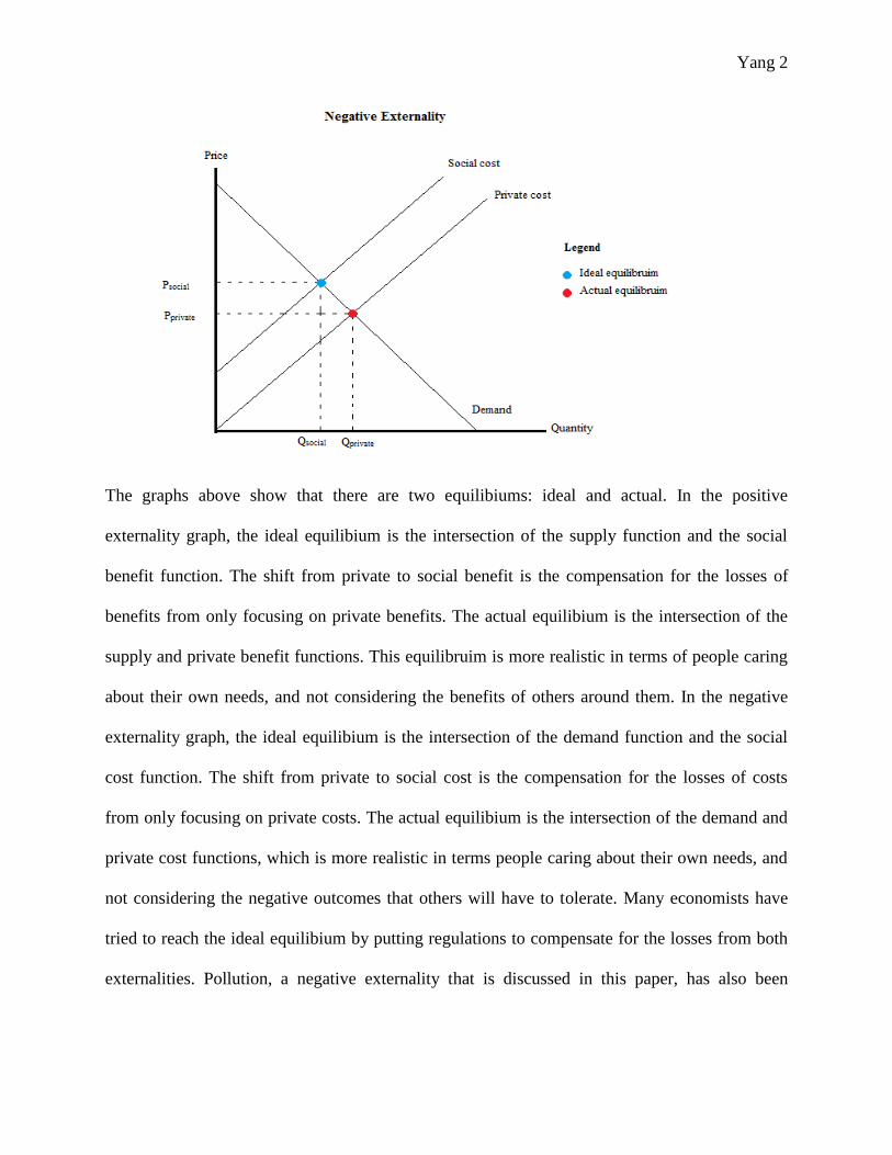
in front of others who do not smoke and they receive second-hand smoking. Here are graphs to

demonstrate positive and negative external effects.

Yang 2

The graphs above show that there are two equilibiums: ideal and actual. In the positive

externality graph, the ideal equilibium is the intersection of the supply function and the social

benefit function. The shift from private to social benefit is the compensation for the losses of

benefits from only focusing on private benefits. The actual equilibium is the intersection of the

supply and private benefit functions. This equilibruim is more realistic in terms of people caring

about their own needs, and not considering the benefits of others around them. In the negative

externality graph, the ideal equilibium is the intersection of the demand function and the social

cost function. The shift from private to social cost is the compensation for the losses of costs

from only focusing on private costs. The actual equilibium is the intersection of the demand and

private cost functions, which is more realistic in terms people caring about their own needs, and

not considering the negative outcomes that others will have to tolerate. Many economists have

tried to reach the ideal equilibium by putting regulations to compensate for the losses from both

externalities. Pollution, a negative externality that is discussed in this paper, has also been

Yang 3

regulated, yet it is inconclusive to decide if the increase in international trade is increasing

pollution levels.

While international trade is increasing, it raises the question: Is international trade

beneficial for the economy and the environment? My hypothesis is that trade and pollution have

a positive relationship—the more trade there is, the more pollution emits to the atmosphere,

leading to more health risks. This prediction ramifies from the pollution-haven hypothesis, which

is one of the most debated topics in international trade and concerns of the environment. The

pollution-haven hypothesis states that because developed countries have higher, stringent

regulations compared to developing countries, this will lead to relocations of factories in

developing countries where regulations are more flexible and thus, lead to cheaper production

costs. However, relocating does not solve the issue of pollution increasing; pollution is only

being moved from one place to another. Overall, these issues are due to firms primarily focusing

on maximizing profits, also known as the market equilibrium. We have not taken into account

the negative externalities that need to be compensated. Many have not realized that the more

production without regulation, the more pollution and wastes we create. When externalities are

neglected, firms are overcompensated—firms do not realize that optimization is only efficient

economically in the short run, but not environmentally in the long run.

Using the U.S. EPA’s RSEI model (Risk Screening Environmental Indicators), data from

U.S. Census Bureau on world trade, and World Bank data on carbon dioxide gas emissions from

manufacturing facilities, I will show time series data, analyzing the correlations over time, gas

emissions due to trade, and tables and graphs showing the relationship between production and

emissions. These are some of the methodologies that will be used to answer my question and

Yang 4

support my hypothesis. I will experiment my hypothesis to see if there is an increase in pollution

levels due to an increase in international trade.

II. Literature Review

“Trade, Growth, and the Environment,” written by scholars Brian R. Copeland and M.

Scott Taylor, lays out the pollution-haven hypothesis, which states that due to strict

environmental policies, firms will relocate to another country where pollution is more tolerable.

This way, firms will not be restricted from producing however many of their goods. Based on

the income effect, if there is an increase in trade and environmental policies, then income will

decrease. This occurs when firms are producing fewer goods but the demands are high. As a

result, many firms lose profits due to stringent regulations, and eventually relocate to an area

where there are more flexible regulations. “Trade may encourage a relocation of polluting

industries from countries with strict environmental policy to those with less stringent policy”

(Copeland & Taylor, 2004). However, this does not solve the issue of pollution, because now it

is not only domestic pollution that we are concerned about—now our concerns incorporate

global pollution. In conclusion, pollution has not been regulated. Instead, it has only been

relocated, and the regulations have been ineffective. However, this is only a speculation that we

perceive if we assume that all firms relocate. In reality, not all firms have the luxury to relocate

to another country, and particular essential resources to produce their goods might not even be in

other countries. Overall, industries cannot relocate to other countries very easily. Therefore, I am

not claiming that trade and environmental regulations are completely useless. In fact, because of

how unrealistic the pollution-haven hypothesis is, trade and environmental policies still do play

essential roles in regulating pollution.

Yang 5

In addition, another literary review by scholars Jaime de Melo, Jean-Marie Grether, and

Nicole A. Mathys also discuss in “Trade, Pollution, and the Environment: New International

Evidence” the pollution-haven effect. Their main research was to see if transportation costs are

expensive enough to prevent the pollution haven effect from occurring. As a result, their

evidence seems to disprove the pollution haven effect. In reference to the bar graph that they

have concocted, it shows that the between-country effect is negative (Grether et al., 2009). This

article also motivated me to look for other externalities on trade, such as the production and

consumption pollution and wastes, and health effects—the aftermath—of pollution. These are

some of the topics that have been ramified to support my hypothesis of trade and pollution

having a positive correlation.

III. Negative Externalities to be Investigated

I will examine the following negative externalities that correspond to international trade

and the effects of the environment: the effects of increased production, the aftermath of increased

consumption, excretion of pollution from transporting goods, and the health consequences due to

pollution. These topics will be individually examined to give us a more explicit picture of what is

happening to the environment based on increased trade levels.

IIIA. Effects of the Environment from Production and Consumption

In order for trade to occur, more goods need to be produced. This can easily be shown by

the Ricardian model. Briefly, the Ricardian model shows us that in order for countries to trade,

every country needs to specialize in what they are most efficient in producing, which is also

known as comparative advantage. In consequence, this drives countries to produce more than the

equilibrium quantity so that not only do they have to support their country, but also to produce

Yang 6

enough to export to other countries. Thus, increase in trade implies that there will also be an

increase in production and consumption. The production of goods also contributes to polluting

the environment. People have believed that trade is economically efficient and helps economic

growth. This implies that if the economy is continuously growing, then there needs to be more

production since not only do we have to produce enough to support the domestic population, but

also for the international population. Therefore, there will be more people consuming goods.

Nevertheless, where do these production and consumption wastes go? Some are shipped and

dumped to other countries that have less environmental quality, some are dumped into the sea,

and some are dumped in other landfills. In addition, some are exposed in the air and cannot be

‘dumped’ anywhere (Kummer, 1994). “Faced with the problem of disposal, more and more

holders of hazardous wastes have, in recent years, chosen to export them from the country of

generation, either for further treatment or final disposal in another country, or for dumping

incineration at sea” (Kummer, 1994, p. 6).

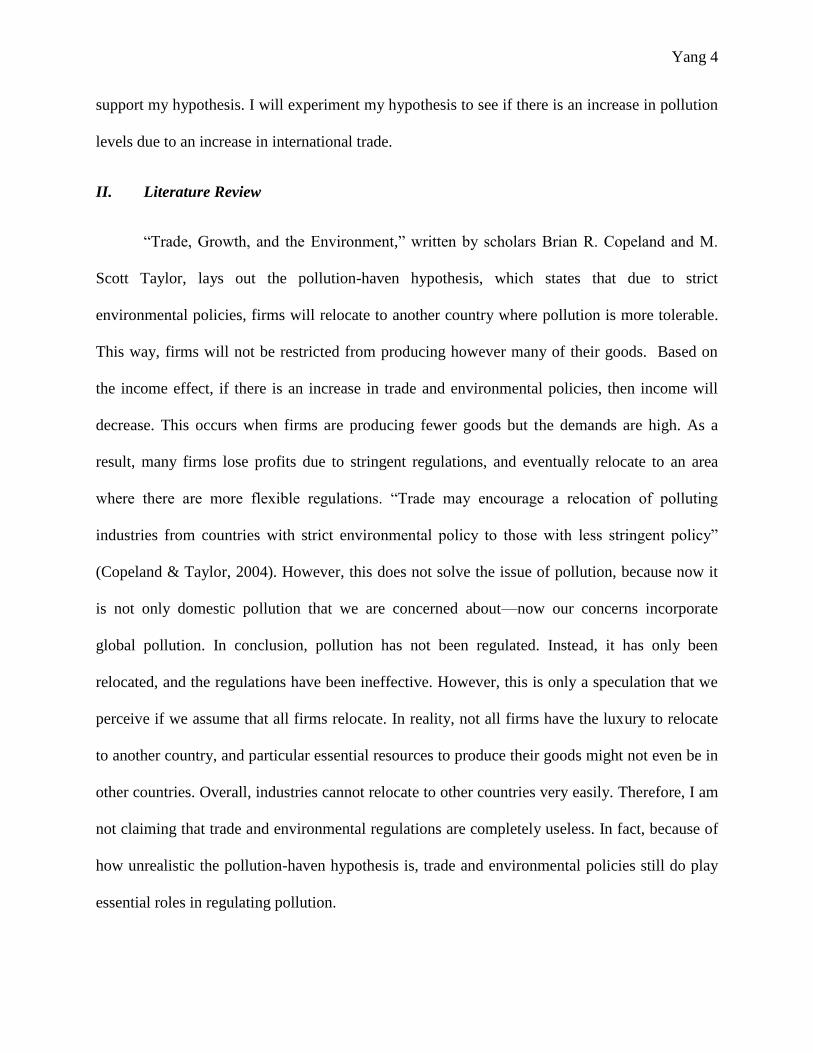
The graph below shows the World Bank’s data on the relationship between time

(measured in years) and the levels of gas emissions, specifically CO2, from burning fossil fuels

and the manufacture of cement (measured in metric tons per capita), also produced from

consumption of solid, liquid, and gas fuels and gas flaring. In addition, I have included the World

Bank U.S. trade data (measured in % GDP). Years 1990 to 2007 have been selected and

observed for both data, since trade was still fairly new in the early 90s and 2007 is the most

recent data that World Bank obtains for both topics. The trend lines are added to show the

correlation between the years and the levels of CO2 emission and trade. We can clearly see that

trade has been increasing by observing the % GDP trend line. Although the trend line is slightly

positive for the CO2 emission levels, the data points seem inconsistent, thus some points have not

Yang 7

contributed to formulating the trend line. Therefore, the increase in CO2 emission levels cannot

be safely concluded.

Although we were not able to conclude the results of the CO2 emission levels increasing,

using the Risk Screening Environmental Indicators (RSEI) model has helped on developing a

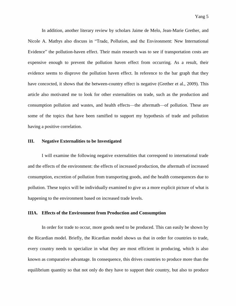
clearer picture of the relationship between trade and levels of emissions. Below, we can look at

the relationship between the monetary value of exports and pounds released by different regions

of the U.S. both in the year 2007. 2007 was chosen to be analyzed since this was the most recent

data that I was able to find in the RSEI model, and in correspondence, I used the 2007 U.S.

Bureau value of exports. There are ten U.S. EPA regions, and all of them have been included

into this graph. The image below the graph is a map of all the U.S. EPA regions

(http://www.epa.gov/acidrain/where/). This will help us interpret the graph below.

18.8

19

19.2

19.4

19.6

19.8

20

20.2

20.4

20.6

0

5

10

15

20

25

30

35

1990 1992 1994 1996 1998 2000 2002 2004 2006

CO

2 E

mis

sio

ns

(met

ric

ton

s p

er c

ap

ita

)

% G

DP

Year

Time Series Data: % GDP and CO2 Emissions

in the U.S.

% GDP CO2 Emissions Linear (% GDP) Linear (CO2 Emissions)

Yang 8

I have concocted a method to make our “Exports vs. Released Emissions from

Manufacturing Facilities by U.S. EPA Regions in 2007” regional analysis more brief and concise:

I divided the graph into three different sectors, and created a category for each of these sectors. I

5

4

6

3

7

2 9 8 1 10

0

200

400

600

800

1000

1200

1400

0 50000 100000 150000 200000 250000 Rel

ea

sed

Em

issi

on

s (b

y m

illi

on

s o

f lb

s.)

Monetary value of Total Exports (by millions of dollars)

Exports vs. Released Emissions from

Manufacturing Facilities

by U.S. EPA Regions in 2007

Yang 9

will call the regions along the x-axis low-concentrated exporting regions, the middle section

fairly-concentrated exporting regions, and the section farthest from the x-axis the highly-

concentrated exporting regions.

According to the graph above, 1, 3, 7, 8, and 10, have the lowest concentrations of

exportation, which also correlates with the released levels of emissions. From my speculation,

region 7 has a low value of exports because based on the inconvenience of their location, they

seem to have the most difficult time exporting goods. They are not on the edges of the U.S., and

Nebraska, Iowa, Kansas, and Missouri do not have congested populations.

Although Regions 2 and 9 are also fairly concentrated in exportation, surprisingly, their

manufacturing facilities release low levels of emissions. My conjecture of this analysis is that

since Region 2 includes New York, a state that is densely populated, many manufacturing

facilities are not built here. The same conjecture goes for Region 9—it includes California; not

only is this state densely populated, but it also has many major cities. Thus, many manufacturing

facilities may not be built here.

The remaining regions, regions 4, 5, and 6, have high concentrations of exportation. Here

are some of my conjectures of why these regions have the highest exports: Region 4 is closest to

some of the Caribbean islands, such as Cuba, Jamaica, The Bahamas, Haiti, Dominican Republic,

and many more. They are most likely to trade with many of the Caribbean islands compared to

the other U.S. states. Region 5 is closest to middle Canada, which makes them to export goods to

Canada most easily compared to other regions. In addition, Michigan is a big shipping zone.

Since Region 6 is closest to Mexico in comparison to other regions, this region can export goods

to Mexico most easily. Overall, the U.S. is able to trade easily with Canada and Mexico, ever

Yang 10

since NAFTA has been established. Analyzing the 2007 graph, we can see that there is a positive

correlation between exports and released emissions.

Although I will not closely examine all ten regions individually, I have selected to choose

a region from each sector to compare their emission and export levels, particularly, 2, 6, and 7.

Region 2 consists of New York, New Jersey, Puerto Rico, and Virgin Islands, Region 6 consists

of New Mexico, Texas, Oklahoma, Arkansas, and Louisiana, and Region 7 consists of Nebraska,

Iowa, Kansas, and Missouri. I have chosen to analyze these particular regions for the following

reasons: Region 2 includes New York, which is one of the most active east coast states in

production and trade, and since Puerto Rico and Virgin Islands are both islands, I assumed that

they trade from various countries and do not produce all goods domestically. Region 6,

especially Texas, is one of the regions closest to Mexico. After finalizing the NAFTA agreement

in 1994, the U.S., especially states closest to Mexico, has frequently traded with Mexico. This

can be observed from the U.S. Census Bureau data in the exports by state section. Based on the

U.S. Census Bureau Exports data, most of Texas’s goods are exported to Mexico. Region 7

includes some of the middle states that are not as active in trade as coastal states. By examining

Region 2 data, we can see that their released pounds are fairly low. Surprisingly, the pounds

released in Region 7 are significantly higher than the pounds released in Region 2. One possible

reason might be that since middle states are not as crowded as costal states such as New York,

more industries are located in these open areas where it is not as congested. However, this is

inconclusive as well. The reasons why emissions are fairly low compared to Region 2 and 7 are

unknown. Nevertheless, we can conclude that the release of emissions is decreasing over time.

This can be due to technology advancement. Many industries may be investing on making their

Yang 11

technology more environmental-friendly, or they might have found alternative materials to use

for production that are degradable.

IIIB. Environmental Effects from Transportation of Goods

There are three main ways that goods are traded and transported among different

countries, and even by regions: air, water, and land. However, seaborne and airborne

transportation contribute to “more than 7% of total global CO2 emissions”

(http://www.epa.gov/international/trade/transport.html). Since increasing trade directly implies

that goods will need to be constantly imported and exported, transportation vehicles will be used

in order to transfer these goods. Transportation vehicles all use polluting oils and fuels in order

to run their engines. The U.S. EPA has been monitoring aircraft on lead emissions, a

carcinogenic chemical, for the past several years. Table 1 shows the airports that had lead

emissions of 0.50 tons or more in 2008 (http://www.epa.gov/otaq/aviation.htm). This table

supports the idea that airplanes emit harmful chemicals when they are flown. Airplanes do not

only emit lead, but they also emit other harmful gases that are dangerous to our health.

Yang 12

This incomplete table is only an example of one of the harmful chemicals that is emitted to the

air. Since transporting goods by sea is another way of emitting greenhouse gases, the U.S. EPA

has also been involved in this regulation. U.S. EPA’s final emission standards are under the

Clean Air Act, which states that new marine diesel engines must be replaced onto ships if the

engines are below 30 liters per cylinder. Although goods are transported by air, water, and land,

on-land vehicles are not usually used for international trade. Instead, they are usually used for

private transportation needs, such as people owning their own cars, or riding on public

transportation. This does not mean that on-land vehicles are not used at all for international

trade—they use trucks to transport goods from one region to another. The Religious Tolerance

organization claim that “a light truck = consumes 813 gallons of gasoline, and emit 108 pounds

of hydrocarbons, 16,035 pounds of CO2, 845 pounds of CO, and 55.8 pounds of nitrogen oxides”

(http://www.religioustolerance.org/tomek33.htm). Although many vehicles are still checked for

smog, there are greenhouse gases emitted. Knowing this, many environmental firms including

the U.S. EPA made a Draft Rule of mandatory reporting of greenhouse gas emissions. Not only

does the Draft Rule focus on monitoring vehicles, but it also focuses on a wide range of other

greenhouse gas sources such as industrial facilities and manufacturers. This means that the Draft

Rule also monitors the air, land, and water vehicles. Having these regulations and monitoring the

detrimental effects of the environment prove that air, water, and land vehicles have been big

contributors to air and water pollution.

Another main claim that (de Melo, Grether, & Mathys, 2009) mentioned in their article is

that the increase in trade will contribute to increase in emissions due to transporting imports and

exports. They have raised the question of whether or not autarky would decrease pollution. If

there was no trade whatsoever, then “opening up to trade leads to an increase of about 10%

Yang 13

(3.5%) in emissions in 1990 (2000)” (Grether et al., 2009). Some of their other reports state that

“international-trade related transport emissions accounted for about 5%-9% of worldwide

manufacturing-related production emissions of SO2—account to roughly one third to three

quarters of total trade-related emissions across the 1990-2000 period” (Grether et al., 2009). In

support of Grether’s Mathy’s, & Melo’s claim, the Religious Tolerance organization has claimed

that oil use increased by 200% since 1973 due to an increase in transportation and in correlation,

emission levels are increasing (http://www.religioustolerance.org/). Particularly, this website

discusses that transporting foods internationally contributes to using more petroleum by four to

seventeen times than if a consumer were to buy the same foods grown and processed locally.

Nonetheless, it is inconclusive to state that the increases in transportation due to trade directly

relate to increases in air and water pollution. Further research needs to be conducted in order to

obtain more concrete data.

IV. Health Effects from Pollution

The main purpose of emphasizing on environmental regulations is the ultimate and

leading consequences of pollution emissions: detrimental health effects. One way health effects

are monitored is using the RSEI model. The RSEI model is not only used to examine the released

emission from different facilities, but it is used to analyze data on released chemicals that might

affect human health risks. RSEI uses information from the Toxics Release Inventory (TRI)

where it computes a risk score that the U.S. EPA uses as an indicator. RSEI is used to see trends

in toxicity of chemicals, releases, and the population affected by the chemical releases. The risk

score is the product of the size of the population, the toxicity weight, and the concentration of the

chemical. The toxicity weight is measured in pounds, and the concentration, also known as

surrogate dose, of the chemical is measured in mg/kg, which indicates that for however many

Yang 14

milligrams of chemicals is exposed in however much a person weighs in kilograms. Hence, risk

scores are usually higher when there is a large population to be considered compared to an area

where there are not as many people exposed to the chemical releases. However, risk scores

would also be high even if there was not a huge population to be considered, if the concentration

of the toxic chemical is high. For example, suppose there are two areas—we will call the first

area A and the second area B. Suppose that Area A has 100 people with a toxic weight of 80

pounds and a surrogate dose of 50 mg/kg, and Area B has 200 people with a toxic weight of 50

pounds and a surrogate dose of 40 mg/kg both have a risk score of 4 x 105. Area A has a higher

toxic weight and surrogate dose than Area B, but Area B has a significantly higher population

which makes up for the ‘losses.’ Hence, risk scores are calculated by the priority of how dense

the population is in certain areas, or how toxic certain emissions are by monitoring how many

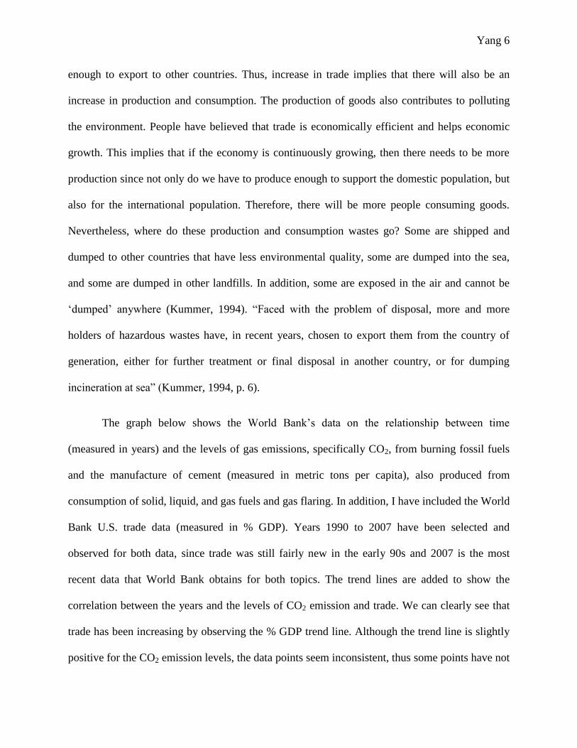
total pounds of emissions are released. Analyzing the following graph, we can see that there is a

positive correlation between released emissions and the risk score.

1 2

3

4

5

6

7

8 9 10

0

5

10

15

20

25

30

35

40

45

50

55

0 100 200 300 400 500 600 700 800 900 1000 1100 1200 1300

Ris

k S

core

(b

y 1

mil

lion

of

un

its)

Released Emissions (by 1 million of pounds)

2007 Released Emissions vs. Risk Score by U.S.

EPA Region

Yang 15

The released emissions include both noncancerous and cancerous chemicals. Nonetheless, a

chemical that is not cancerous does not imply that it does no harm to organisms and the

environment. Therefore, the U.S. EPA have been monitoring and researching all chemicals to see

the effects of organisms depending on how high the level of exposure is. An example of a

noncancerous chemical is CO2. However, this chemical gives us cancer indirectly: Excess CO2

deteriorates the ozone (O3) layer, a necessary outer layer that protects us from harmful ultraviolet

rays. Frequently being exposed to ultraviolet rays lead to skin cancer, declination of the immune

system, and eye cataracts. An example of a carcinogenic chemical is lead, which was mentioned

in Section IIIB. Consuming and inhaling lead have many detrimental health effects, such as

damages to the central and peripheral nervous system, increased blood pressure, hearing and

vision impairment, reproductive problems, defects of fetal development, brain damage, mental

retardation, liver and kidney damage, delays in development, anemia, and in extreme cases, even

death (http://www.epa.gov/superfund/health/contaminants/lead/health.htm#Health%20Concerns).

As we can see, people have been affected by pollution implicitly and explicitly, thus

environmental regulations have been created.

V. Conclusion

Attempting to find the direct relationship between international trade, pollution, and

health effects is difficult, since many other factors and variables have not been included in my

models. However, if we were to relate them in a simplistic manner, then by observing the

increase in % GDP in the U.S., trade is increasing. Additionally, the results of the relationship

between exports and released emissions show that there is a positive correlation. Lastly, the

increase in emissions also gives us higher risk scores, meaning that there are increased

detrimental health effects due to an increase in pollution. However, all of these do not imply that

Yang 16

all countries should abide to autarky. By looking at the World’s % GDP on the World Bank

website, we can see that there is an increase in % GDP, meaning that international trade

promotes economic growth (http://search.worldbank.org/all?qterm=trade). Therefore, as long as

we find the right balance of environmental regulation while promoting economic growth,

international trade is beneficial.

Yang 17

References

Aircraft. (n.d.). Retrieved January 26, 2011, from http://www.epa.gov/otaq/aviation.htm

Copeland, B.R. & Taylor, M. S. (2004). Trade, Growth, and the Environment.

[Electronic version]. Journal of Economic Literature, 7-71.

Grether, J., Mathys, N.A., & de Melo, J. (2009, November). Trade, pollution, and the

environment: New international evidence. Vox. Retrieved February 1, 2011, from

http://voxeu.org/index.php?q=node/4308

Human Health. (n.d.). Retrieved March 7, 2011, from

http://www.epa.gov/superfund/health/contaminants/lead/health.htm#Health%20Concerns

Kummer, K. (1994). Transboundary Movements of Hazardous Wastes at the Interface of

Environment and Trade. Geneva, Switzerland: Environment and Trade UNEP.

Ocean Vessels and Large Ships. (n.d.). Retrieved January 26, 2011, from

http://www.epa.gov/otaq/oceanvessels.htm

Pollution caused by land travel, air travel, and food transportation. (n.d.). Retrieved

March 5, 2011, from http://www.religioustolerance.org/tomek33.htm

Risk Screening Environmental Indicators. (n.d.). Retrieved February 22, 2011, from

http://www.epa.gov/opptintr/rsei/pubs/tech_info.html

State Trade Data. (n.d.). Retrieved February 24, 2011, from

http://www.census.gov/foreign-trade/statistics/state/

Trade, Transportation, and the Environment. (n.d.). Retrieved January 26, 2011, from

http://www.epa.gov/international/trade/transport.html

World Bank Trade data. (n.d.). Retrieved March 4, 2011, from

http://search.worldbank.org/all?qterm=trade