Kyoto University, Graduate School of Economics Research Project Center Discussion Paper Series

Trade Patterns and International Technology Spillovers:

Theory and Evidence from Patent Citations

Naoto Jinji

Xingyuan Zhang Shoji Haruna

Discussion Paper No. E-10-006

Research Project Center Graduate School of Economics

Kyoto University Yoshida-Hommachi, Sakyo-ku Kyoto City, 606-8501, Japan

October 2010

Trade Patterns and International Technology Spillovers:

Theory and Evidence from Patent Citations∗

Naoto Jinji† Xingyuan Zhang‡ Shoji Haruna§

This version: March 28, 2011

Abstract

In this paper, we develop a two-country model of monopolistic competition with quality dif-

ferentiation by extending the model of Melitz and Ottaviano (2008) and examine the relationship

between the bilateral trade structure and international technology spillovers. We show that bilat-

eral trade patterns and the extent of technology spillovers will change, depending on the technology

gap between two countries. We then test predictions of the model by using bilateral trade data

among 44 countries and patent citation data at the U.S., European, and Japanese Patent Offices.

We use patent citations as a proxy for spillovers of technological knowledge. Trade patterns are

categorized into three types: one-way trade (OWT), horizontal intra-industry trade (HIIT), and

vertical intra-industry trade (VIIT). Each of OWT and VIIT is further divided into two sub-

categories, based on the direction of trade. We find that intra-industry trade plays a significant

role in technology spillovers. In particular, HIIT is associated with larger technology spillovers

than VIIT, which confirms the predictions of the model.

Keywords: technology spillovers; patent citations; intra-industry trade; firm heterogeneity.

JEL classification: F12; O31; O33.

∗We would like to thank Lee Branstetter, Shuichiro Nishioka, Nobuhito Suga and seminar and conference partici-

pants at Kyoto University, Hokkaido University, Otaru University of Commerce, University of Pittsburgh, Yokohama

National University, APTS 2010, Fall 2010 Meeting of Midwest International Economics, Korea International Economic

Association meeting 2010 for their helpful comments and suggestions on earlier versions of the paper. We alone are

responsible for any remaining errors. We acknowledge financial support from the Japan Society for the Promotion of

Science under the Grant-in-Aid for Scientific Research (B) No. 19330052 and the Murata Science Foundation.†Corresponding author. Faculty of Economics, Kyoto University, Yoshida-honmachi, Sakyo-ku, Kyoto 606-8501,

Japan. Phone & fax: +81-75-753-3511. E-mail: jinji #at-mark# econ.kyoto-u.ac.jp.‡Faculty of Economics, Okayama University, 3-1-1 Tsushima-Naka, Kita-Ku, Okayama 700-8530, Japan.§Faculty of Economics, Okayama University, 3-1-1 Tsushima-Naka, Kita-Ku, Okayama 700-8530, Japan.

1

1 Introduction

The issue of international technology diffusion has been attracted great attention in economics.1 This

is because international technology diffusion is an important factor to determine the speed at which

the world’s technology frontier expands. It also contributes to income convergence across countries.

For example, Eaton and Kortum (1996) estimate innovation and technology diffusion among 19

OECD countries to test predictions from a quality ladders model of endogenous growth with patenting.

They find that each OECD country other than the United States (U.S.) obtains more than half of

its productivity growth from technological knowledge originated abroad. They also find that more

than half of the growth in every OECD country is derived from innovation in the U.S., Japan, and

Germany. Eaton and Kortum (1999) fit a similar model to research employment, productivity, and

international patenting among the five leading research economies, i.e., the U.S., Japan, Germany, the

United Kingdom (U.K.), and France. They find that research performed abroad is about two-thirds as

potent as domestic research. In particular, technological knowledge from Japan and Germany diffuses

most rapidly, while France and Germany are the quickest to exploit knowledge. They also show that

the U.S. and Japan together contribute to over 65 percent of the growth in each of the five countries.

Previous studies have identified international trade as a major channel of international technology

spillovers.2 Coe and Helpman (1995) examine R&D spillovers among OECD countries and find large

spillover effects from foreign R&D capital stocks to domestic productivity that is measured by total

factor productivity (TFP). They also show that countries exhibit higher productivity levels by im-

porting goods from countries with high levels of technological knowledge, which supports the existence

of trade-related international R&D spillovers. However, Keller (1998) provides a finding that casts

doubt on Coe and Helpman’s result by employing a Monte-Carlo-based robustness test. He finds that

estimated international R&D spillovers among randomly matched trade partners turn out to be large

(and even larger than those among actual trade partners). Xu and Wang (1999) estimate that about

half of the return on R&D investment in 7 OECD countries spilled over to other OECD countries and

that trade in capital goods is a significant channel of R&D spillovers. More recent study by Acharya

and Keller (2009) find that the diffusion of technological knowledge is strongly varying across country-

pairs. They show that imports are crucial for technology diffusion from Germany, France, and the

U.K., while non-trade channels are relatively more important for the U.S., Japan, and Canada.

1See Keller (2004) for a survey of the literature.2Trade works as a channel of technology spillover because, for example, firms can obtain information on advanced

technology by reverse engineering of imported goods. International trade also provides channels of cross-border com-

munication that facilitates learning of production and organizational methods and market conditions (Grossman and

Helpman, 1991). Another major channel is foreign direct investment (FDI). Technological spillovers through FDI are

empirically confirmed by a number of studies (Branstetter, 2006; Haskel, Pereira, and Slaughter, 2007; Javorcik, 2004;

Keller and Yeaple, 2009), while some studies do not find significant spillovers (Aitken and Harrison, 1999; Haddad and

Harrison, 1993).

2

Although a number of studies have investigated technological knowledge spillovers through trade,

none of the existing studies have paid attention to the relationship between bilateral trade patterns and

technology spillovers. However, it is expected that technology spillovers through imports will differ,

depending on whether a country exports products with similar quality or with different quality in the

same industry as imports or the country does not export products in the same industry. Therefore, in

this paper we examine the relationship between the bilateral trade structure and technology spillovers

from both theoretical and empirical points of view. Here, by the term “technology spillovers” we refer

to “the process by which one inventor learns from the research outcomes of others’ research projects

and is able to enhance her own research productivity with this knowledge without fully compensating

the other inventors for the value of this learning” (Branstetter, 2006: 327–328). In this sense, we

distinguish technology spillovers from imitation or technology adoption.

Empirical studies on intra-industry trade categorize bilateral trade flows into one way trade

(OWT), or inter-industry trade, and two-way trade, or intra-industry trade (IIT). IIT is further

decomposed into horizontal intra-industry trade (HIIT) and vertical intra-industry trade (VIIT) (e.g.,

Fontagne and Freudenberg, 1997; Greenaway, Hine, and Milner, 1995; Fukao, Ishido, and Ito, 2003).

The difference between HIIT and VIIT reflects the differences in quality of products in the same

category traded between two countries. In HIIT, horizontally differentiated products (i.e., products

with similar quality but different varieties) are traded, whereas vertically differentiated products (i.e.,

products with different qualities) are traded in VIIT.3 On data HIIT and VIIT can be distinguished

by using unit values (i.e., total value of import or export in one product category divided by quantity

of import or export in that product category) under the assumption that unit values are increasing

in product quality.

The theoretical literature on intra-industry trade has been separated into two branches for a long

period. As is well known, trade models with monopolistic competition could explain HIIT (e.g., Krug-

man, 1979, 1980; Helpman, 1981; Eaton and Kierzkowski, 1984). However, in these models, product

varieties are symmetric and not differentiated in quality. Trade models with vertical differentiation, on

the other hand, could explain VIIT but could not explain HIIT (e.g., Falvey, 1981; Shaked and Sutton,

1984; Falvey and Kierzkowski, 1987; Flam and Helpman, 1987; Lambertini, 1997; Motta, Thisse, and

Cabrales, 1997; Herguera and Lutz, 1998). Given the fact that HIIT and VIIT arise in continuous

phenomena, this divergence in the theory would not be acceptable. More recently, a number of studies

have attempted to introduce quality differentiation into the monopolistically competitive trade model.

Some studies use a quality-augmented type of Dixit-Stiglitz demand specification in the framework

3Note that in the literature the terms of HIIT and VIIT are sometimes used in different meanings. In an alternative

definition, HIIT means trade of final goods in the same industry across countries, while VIIT involves trade of interme-

diate goods with final goods in the same industry (Yomogida, 2004). Since we do not consider the distinction between

intermediate goods and final goods in this paper, this alternative definition of HIIT and VIIT is not applicable.

3

of Melitz (2003)4 with the assumption that higher quality is associated with higher marginal cost

(Baldwin and Harrigan, 2007; Gervais, 2008; Helble and Okubo, 2008; Johnson, 2010; Kugler and

Verhoogen, 2010; Mandel, 2010).5 On the other hand, Antoniades (2008) introduces quality differ-

entiation into the quasi-linear utility with a quadratic subutility specification in the framework of

Melitz and Ottaviano (2008) and considers endogenous quality upgrading by heterogeneous firms. He

shows that firms with higher productivity choose higher qualities and charge higher prices. However,

his model faces some limitations when extended to the case of two-country trade. In this paper, we

also introduce quality differentiation into the framework of Melitz and Ottaviano (2008). We employ

a different approach from Antoniades (2008). We assume that firms randomly draw their product

quality so that firms with identical productivity are heterogeneous in product quality. This reflects

the stochastic nature of product R&D. This formulation of quality differentiation turns out to be

tractable. Then, we show that our model can explain OWT, HIIT, and VIIT in one unified frame-

work. Using this framework, we examine how international technology spillovers are associated with

bilateral trade structure.

For empirical analysis of international technology spillovers, we use data on patent citations as a

proxy for spillovers of technological knowledge. There is a relatively small but growing literature on

empirical analysis of knowledge flow based on patent citations (e.g., Jaffe, Trajtenberg, and Henderson,

1993; Jaffe and Trajtenberg, 1999; Hu and Jaffe, 2003; MacGarvie, 2006; Mancusi, 2008; Haruna, Jinji,

and Zhang, 2010).6 In the literature, patent citation data are used as a direct measure of technology

spillovers (Hall, Jaffe, and Trajtenberg, 2001). Hu and Jaffe (2003) use data on patents granted in

the U.S. and examine patent citations by inventors residing in Korea, Japan, Taiwan, and the U.S.

to infer the pattern of technological knowledge flows from the U.S. and Japan to Korea and Taiwan.

They find that Korean patents are much more likely to cite Japanese patents than U.S. patents, while

Taiwanese patents cite both Japanese and U.S. patents evenly. Mancusi (2008) estimates technological

knowledge diffusion within and across sectors and countries by using European patents and citations

for 14 OECD countries. She finds that international knowledge diffusion is effective in increasing

innovative productivity in technologically laggard countries, while technological leaders (the U.S.,

Japan, and Germany) are a source rather than a destination of knowledge flows. Using French firms’

patent citations and firm-level trade data, MacGarvie (2006) finds that the patents of importing firms

4Originally, Melitz (2003) mentions that differences in productivity may be interpreted as differences in product

quality at equal cost.5Sugita (2010) also uses a quality-augmented type of Dixit-Stiglitz demand and considers matching between inter-

mediate good producers and final good producers. He shows that improvements in matching due to trade liberalization

result in improvements in product quality.6However, Jaffe, Trajtenberg, and Henderson (1993) admit that patent citation is a coarse and noisy measure

of knowledge flow, because not all inventions are patented and not all knowledge flows can be captured by patent

citations. Based on a survey of inventors, Jaffe, Trajtenberg, and Fogarty (2000) suggest the validity of patent citations

as indicators of technology spillovers, despite the presence of noise.

4

are significantly more likely to be influenced by technology in the exporting country than are the

patents of firms that do not import. In contrast, she finds no significant evidence of exporting firms’

citing more patents from their destination countries. Moreover, in our previous work (Haruna, Jinji,

and Zhang, 2010), we investigate whether the trade structure plays an important role as a channel

of technological knowledge diffusion between Asian economies (Korea, Taiwan, China, and India)

and G7 countries including the U.S. and Japan. In that paper, we use a modified version of the

Balassa’s index of Revealed Comparative Advantage (RCA), which represents the share of country i

in sector j relative to the country’s export (or import) share for all sectors. Then, we find that trade

specialization, especially import specialization, has a direct effect on knowledge diffusion.

In this paper, we take our study one step further and investigate the relationship between bilateral

trade patterns and international knowledge flow in more detail. In order to accomplish this task,

we develop a two-country model of monopolistic competition with quality differentiation, in which

inter- and (horizontal and vertical) intra-industry trade patterns endogenously arise, depending on

the conditions of trading countries. Our model is an extension of the model developed by Melitz and

Ottaviano (2008). In our model, firms are heterogeneous in product quality rather than in productivity.

Then, after deriving hypotheses from the model, we test them by using data on bilateral trade among

44 countries and patent citations at the U.S., European, and Japanese Patent Offices.

The main results in this paper are as follows. Our model predicts that the bilateral trade pattern

is HIIT when the two countries have access to a similar level of technology, while it is VIIT when

there is technological difference between them. Moreover, if the technological difference is sufficiently

large, the bilateral trade pattern becomes OWT. Our model also predicts that technology spillovers

are highest when the bilateral trade pattern is HIIT, followed by VIIT and OWT. Our estimation

results basically confirm those predictions of the model. We find that an increase in the share of intra-

industry trade in the bilateral trade has a positive effect on the number of patent citations between

the two countries. HIIT has a larger effect than VIIT. On the other hand, the effects of OWT on the

number of citations are much weaker than those of IIT.

The remainder of the paper is organized in the following way. Section 2 sets up a closed-economy

model of monopolistic competition with quality differentiation. Section 3 extends the model to the

case of two-country trade and derives testable implications from the theoretical model. Section 4

conducts an empirical analysis. Section 5 concludes this paper.

5

2 The Basic Model

In this section, we describe the basic structure of the model in a closed economy. Then, we extend

the basic model to the case of two-country trade in the next section.

Consider an economy with two sectors: a homogenous agricultural sector and a differentiated

manufacturing sector.7

2.1 Demand

We introduce quality differentiation into the quasi-linear (instantaneous) utility with a quadratic

subutility, which is developed by Ottaviano, Tabuchi, and Thisse (2002) and Melitz and Ottaviano

(2008).8 There are L consumers in the economy. Preferences are identical across consumers and

defined over a continuum of differentiated varieties indexed by i ∈ Ω and a homogenous numeraire

good. The representative consumer maximizes an additively separable intertemporal utility function

of the form,

U =∫ ∞

0

u(t)e−ρtdt, (1)

where ρ is the common subjective discount rate and u(t) is the instantaneous utility given by

u(t) = qc0t +

∫i∈Ωt

αitqcitdi − 1

2γ

∫i∈Ωt

(qcit)

2di − 12η

(∫i∈Ωt

qcitdi

)2

, (2)

where qc0t and qc

it are the individual consumption levels of the numeraire and variety i at time t and

αit > 0 measures the product quality of variety i at time t.9 The parameter γ > 0 measures the

degree of horizontal differentiation, or the substitutability between varieties and the parameter η > 0

captures the degree of substitution between the differentiated varieties and the numeraire.

We assume that consumers have positive demands for the numeraire. The inverse demand for

variety i at time t is then given by

pit = αit − γqcit − ηQc

t , (3)

as long as qcit > 0, where Qc

t =∫

i∈Ωtqitdi is the total consumption level over all varieties. Let Ω∗

t ⊂ Ωt

be the subset of varieties that are actually consumed. Then, from Eq. (3), the market demand for

variety i ∈ Ω∗t can be expressed as

qit ≡ Lqcit =

L

γαit − ηLNt

γ(ηNt + γ)αt − L

γpit +

ηLNt

γ(ηNt + γ)pt, (4)

7In this section, we develop a simple two-sector model. The analysis can be extended to a model with many

differentiated manufacturing sectors to fit the empirical study in the next section. However, such an extension will not

change qualitatively the main results in this section.8The quadratic utility is also widely employed for the analysis of oligopoly. See, for example, Dixit (1979), Singh and

Vives (1984), and Vives (1985). Quality-augmented versions of the quadratic utility function are developed by recent

studies of Hackner (2000) and Symeonidis (2003a, 2003b).9Hackner (2000) provides the same treatment of product quality in a discrete version of quadratic utility.

6

where Nt is the measure of consumed varieties in Ω∗t , and αt = (1/Nt)

∫i∈Ω∗

tαitdi and pt =

(1/Nt)∫

i∈Ω∗tpitdi are their average quality and price, respectively.

2.2 Supply

In both sectors, labour, which is inelastically supplied in the competitive labour market, is the only

production factor. One unit of labour is required to produce one unit of the homogenous agricultural

(numeraire) good. Thus, the wage rate w is equal to one.

In the differentiated manufacturing sector, each firm produces a different variety. Every product

variety has generations (or versions), depending on the date of development. For simplicity, we assume

that each generation of a product variety loses its consumption value after one period. Thus, each

firm must engage in product R&D to develop a new generation of the product variety in every period.

While the cost of product R&D, f (measured in units of labour), is identical for all manufacturing

firms, the outcome of product R&D, αit, is stochastic.10 Since R&D actually involves uncertainty in

its outcome, it would be quite natural to model R&D as a stochastic process. To simplify the analysis,

we model product R&D in the following way. Let αMt be the maximum product quality that could be

obtained by the current technology in the economy, or the frontier of the current technology, at time

t. Firm i randomly draws the degree of successfulness of R&D, ait, from a time-invariant common

(and known) probability density function g(a) with support on [a, 1], where 0 < a. We assume that

g′(a) < 0 so that the probability of higher degree of success is lower. Then, firm i’s product quality

is given by αit = aitαMt. This implies that the product R&D can be equivalently expressed as a

random draw from a cumulative distribution function Gt(α) with support on [αt, αMt] at time t,

where αt = aαMt. As is explained below, Gt(α) shifts as time passes. We normalize that αM0 = 1.

That is, let the maximum quality of the first generation of the product be one.

Each firm must decide whether to spend the cost of R&D before knowing its outcome. If a firm

does not conduct R&D at time t, it does not enter the market in that period.

The market competition in the manufacturing sector takes a form of three-stage game. In stage

one, all potential entrants decide whether to engage in product R&D (by paying the cost of f). In

stage two, those firms conducted R&D in the previous stage know the outcome of R&D and then

decide whether to stay in the market or exit. In stage three, the firms that stay in the market choose

prices to maximize their own profits.11

A variety of the manufacturing good is produced under constant-returns-to-scale at unit labour

requirement c, which is identical across all firms and independent of the product quality αit.12 Since10As is evident, the cost of product R&D f serves as a fixed entry cost. Since firms pay a fixed entry cost and draw

their productivity parameter in Melitz (2003) and Melitz and Ottaviano (2008), firms engage in stochastic process R&D

in their cases. In our model, on the other hand, firms engage in stochastic product R&D.11In the two-country model in Section 3, each firm chooses price in each market independently.12We assume identical productivity across all firms to simplify the analysis. Our model can be extended to incorporate

7

w = 1 as long as the numeraire good is produced in the economy, c is the (constant) marginal cost.

Since the R&D cost is sunk, firms that can cover their marginal costs survive and supply manufacturing

goods to the market. All other firms exit. Surviving firms maximize their profits in each period by

taking the average quality level α, the average price level p, and the number of firms N in that

period as given.13 Given the market demand for variety i (Eq. (4)), it is easily seen that the price

elasticity of demand, εi ≡ −(∂qi/∂pi)(pi/qi), does not tend to infinity as N goes to infinity. Thus,

the manufacturing sector is characterized by monopolistic competition.14 Let pmax(α) be the price

at which demand for a variety with quality α is driven to 0. Eq. (4) yields that

pmax(α) ≡ α − ηN

ηN + γ(α − p). (5)

Then, any i ∈ Ω∗ satisfies pi ≤ pmax(αi). Given Eq. (4), firm i’s gross profit is given by πi = piqi−cqi.

From the first-order condition (FOC) for profit maximization, we obtain

q(α) =L

γ[p(α) − c], (6)

where q(α) and p(α) are profit-maximizing output and price for the product with quality α. Let αD

be the quality level for the firm that earns zero profit due to p(αD) = pmax(αD) = c. Using Eq. (5),

it yields that

αD =ηN

ηN + γ(α − p) + c. (7)

Then, substitute Eq. (4) into Eq. (6) and use Eq. (7) to obtain

p(α) =α − αD

2+ c. (8)

This implies that firms with positive demands (i.e., αi > αD) charge prices above the marginal cost

and that the prices are increasing in product quality. Note that the average price p is given by

p =α − αD

2+ c. (9)

Then, (7) and (9) yield the mass of surviving firms

N =2γ(αD − c)η(α − αD)

. (10)

Note that the average product quality of surviving firms α is expressed as α = [∫ αM

αDαdGt(α)]/[1 −

Gt(αD)] and that the mass of entrants is given by NE = N/[1 − Gt(αD)].

Although we do not use a specific parametrization for the distribution Gt(α), we assume the

following condition:heterogeneous productivity among firms, like Melitz (2003) and Melitz and Ottaviano (2008).

13Hereafter, we omit the time index unless necessary.14In contrast to the standard model of monopolistic competition with constant elasticity of substitution (CES) demand

developed by Dixit and Stiglitz (1977), the price elasticity of demand is not uniquely determined by the degree of

product differentiation in this quasi-linear utility with quadratic subutility specification. Behrens and Murata (2007)

and Zhelobodko, Kokovin, and Thisse (2010) also investigate implications of relaxing the CES assumption in the

monopolistic competition.

8

Assumption 1 0 < dα/dαD < 1.

This condition means that an increase in the cut-off quality increases the average quality of products

supplied in the market but the extent of the increase in the average quality is smaller than the

increase in αD. This condition restricts the shape of the distribution Gt(α). We need this assumption

to obtain an unambiguous effect of a change in the cut-off product quality on the size of product

varieties, which will be shown below. Note that in Melitz and Ottaviano (2008) a similar property

holds for the relationship between the cut-off productivity and the average productivity by assuming

a Pareto distribution for the distribution of cost draws.

Following Melitz and Ottaviano (2008), let μ(α) = p(α) − c, r(α) = p(α)q(α), and π(α) = r(α) −q(α)c be the absolute mark-up, revenue, and profits of a firm that produces a product with quality α.

Then, these performance measures can be written as

μ(α) =α − αD

2, (11)

q(α) =L(α − αD)

2γ, (12)

r(α) =L

4γ

((α − αD)2 + 2c(α − αD)

), (13)

π(α) =L

4γ(α − αD)2. (14)

Since the expected profit prior to entry at time t is given by∫ αM

αDπ(α)dGt(α)− f , the equilibrium

free entry condition is given by∫ αM

αD

π(α)dGt(α) =L

4γ

∫ αM

αD

(α − αD)2dGt(α) = f. (15)

The first equality is obtained by using Eq. (14). From Eqs. (10) and (15), we obtain the following

lemma:

Lemma 1 (i) Given Gt(α), αD and α are both decreasing in f (R&D cost) and γ (the degree of

horizontal differentiation) and increasing in L (the market size).

(ii) Under Assumption 1, for a given Gt(α), a higher αD leads to a higher N (more varieties) and a

higher NE (more entrants).

Proof. The first part is directly obtained from Eq. (15). For the second part, differentiate Eq. (10)

with respect to αD to yield

dN

dαD=

2γ

η(α − αD)− 2γ(αD − c)

η(α − αD)2d(α − αD)

dαD> 0.

Assumption 1 ensures that the right-hand-side is positive. Then, since NE = N/[1−Gt(αD)], a higher

αD and a higher N lead to a higher NE .

9

This lemma shows that the effects of parameters on the cut-off quality and the average quality

in our model are similar to the effects of parameters on the cut-off productivity and the average

productivity in Melitz and Ottaviano (2008).

2.3 Technology spillovers

The individual firm’s technological knowledge spillovers to other firms in the manufacturing sector.

In the spirit of Romer (1990) and Grossman and Helpman (1990, 1991), we assume that technological

knowledge has a public-good nature. That is, individual firm’s R&D output contributes to “general

knowledge” in the economy and all firms equally have access to the general knowledge without any

costs. We capture technology spillovers by the expansion of the technology frontier, αMt. More

specifically, we assume that αMt changes in the following way:

αMt = λKtαMt, (16)

where λ > 0 and Kt is the knowledge flow at time t. Assuming that knowledge flow is proportional

to the number of varieties actually produced, we have

Kt = Nt (17)

by choosing units for Kt. Note that Nt is the mass of surviving firms that produces quality level

α ≥ αDt.

Since technology spillovers shift the distribution G(α) to the right without changing its shape, it

has the following properties:

Lemma 2 An upward shift of G(α) leaves μ(α), q(α), r(α), and π(α) unchanged and increases N

and NE.

Proof. Let G0(α0) and G1(α1) be the distributions before and after the change, respectively. Let

α0M and α1

M be the upper bound of G0(α0) and G1(α1), respectively, and set α1M = α0

M + k with

k > 0. Then, since α1 = α0 + k holds for any α0 and α1 that take the same relative position in each

distribution, Eq. (15) for G0(α0) can be transformed to that for G1(α1). Thus, Eqs. (11) to (14) are

unchanged. However, since α − αD is unchanged and α1D = α0

D + k, Eq. (10) yields a higher N and

hence a higher NE .

This lemma implies that as long as all firms equally have access to the general knowledge, tech-

nology improvement in the sense of an upward shift of G(α) increases the absolute levels of product

quality for all varieties but keeps their relative positions in the industry unchanged. However, Lemma

2 also implies that there are more varieties in the economy with advanced technology than in the

economy with lagged technology.

10

3 Trade between Two Countries

3.1 A two-country setting

Now, we consider two countries, Home and Foreign with LH and LF consumers in each country.

Consumers in both countries share the same preferences given by Eqs. (1) and (2). We assume that

the markets in the two countries are segmented, while firms can produce in one location and supply

their products to the market in the other country by incurring a per-unit trade cost.

Manufacturing firms in the two countries have the same marginal cost c but draw product qualities

αH and αF from their domestic distributions GHt (α) and GF

t (α) with support on [αHt , αH

Mt] and

[αFt , αF

Mt], respectively.

Following Melitz and Ottaviano (2008), we assume that firms in country h must incur the unit

cost of τ lc with τ l > 1 to deliver one unit of their products to the market in the country l. We also

assume that the homogenous numeraire good is always produced in each country after opening up to

trade, so that the wage rate is equal to one in both countries.

The price threshold for positive demand in market l is given by

plmax(α) ≡ α − ηN l

ηN l + γ(αl − pl), (18)

where N l is the mass of firms selling in country l, which includes both domestic firms in country l

and exporters from country h, and αl and pl are respectively average quality and price across both

local and exporting firms in country l. Let N lD and N l

X denote the mass of firms producing in country

l that supply products to the domestic market and the other country’s market, respectively. Then,

N l = N lD + Nh

X holds (l, h = H, F, l �= h).

Firms maximize their profits earned from local and export sales independently (due to the assump-

tions of segmented market and constant-returns-to-scale technology). Let αlD and αl

X be the quality

levels for the firm producing in country l that earns zero profits from local sales and export sales,

respectively. From p(αlD) = pl

max(αlD) = c and p(αl

X) = phmax(αl

D) = τhc, we obtain

αlD =

ηN l

ηN l + γ(αl − pl) + c, (19)

αlX =

ηNh

ηNh + γ(αh − ph) + τhc. (20)

Thus, it holds that

αhX = αl

D + (τ l − 1)c. (21)

Let πlD(α) = [pl

D(α)− c]qlD(α) and πl

X(α) = [plX(α)− τhc]ql

X(α) be the maximized value of profits

for a firm with quality α producing in country l from domestic sales and export sales, respectively,

where plD(α) and pl

X(α) are profit-maximizing prices for domestic and export sales, respectively,

and qlD(α) and ql

X(α) are corresponding quantities. From the first-order conditions, it holds that

11

qlD(α) = (Ll/γ)[pl

D(α)−c] and qlX(α) = (Lh/γ)[pl

X(α)−τhc]. Then, use the same procedure to derive

(9) and (12) in the closed economy to yield the optimal prices and outputs for domestic and export

sales, respectively:

plD(α) =

α − αlD

2+ c, ql

D(α) =Ll(α − αl

D)2γ

, (22)

plX(α) =

α − αlX

2+ τhc, ql

X(α) =Lh(α − αl

X)2γ

. (23)

Then, the maximized profits from domestic sales and export sales are respectively given by

πlD(α) =

Ll

4γ(α − αl

D)2, (24)

πlX(α) =

Lh

4γ(α − αl

X)2. (25)

The equilibrium free entry condition in country l at time t is given by

∫ αlMt

αlDt

πlD(α)dGl

t(α) +∫ αl

Mt

αlXt

πlX(α)dGl

t(α) = f. (26)

Substitute (21), (24), and (25) into this to yield two equilibrium free entry conditions:

LH

∫ αHMt

αHDt

(α − αH

Dt

)2dGH

t (α) + LF

∫ αHMt

αFDt

+(τF−1)c

[α − αF

Dt − (τF − 1)c]2

dGHt (α) = 4γf,(27)

LF

∫ αFMt

αFDt

(α − αF

Dt

)2dGF

t (α) + LH

∫ αFMt

αHDt

+(τH−1)c

[α − αH

Dt − (τH − 1)c]2

dGFt (α) = 4γf,(28)

which jointly determine the cut-off qualities for domestic sales in the Home and Foreign at time t,

αHDt and αF

Dt. We then assume the following:

Assumption 2∫ αl

M

αl

πlD(α)dGl(α) +

∫ αlM

αl

πlX(α)dGl(α) > f .

Under Assumption 2, there are always some firms that exit the market in country l even if no firm

enters the market in country h.

Since the mass of firms selling in country l at time t is still determined by (10), N lt is given by

N lt =

2γ(αlDt − c)

η(αlt − αl

Dt), (29)

where αlt is the average quality of products sold in country l at time t, which is given by

αlt =

∫ αlMt

αlDt

α dGlt(α) +

∫ αhMt

αlDt

+(τ l−1)cα dGh

t (α)

2 − Glt(αl

Dt) − Ght (αl

Dt + (τ l − 1)c).

Similar to Assumption 1 in the case of the closed economy, we assume

Assumption 3 0 < dαl/dαlD < 1.

12

Let N lEt be the mass of entrants producing in country l at time t, which is determined by

[1 − GHt (αH

Dt)]NHEt + [1 − GF

t (αFXt)]N

FEt = NH

t , (30)

[1 − GFt (αF

Dt)]NFEt + [1 − GH

t (αHXt)]N

HEt = NF

t , (31)

where [1 − Glt(α

lDt)]N

lEt = N l

Dt and [1 − Glt(α

lXt)]N

lEt = N l

Xt. The equilibrium free entry conditions

(27) and (28) will hold so long as there is a positive mass of entrants N lEt > 0 in country l at time t.

Otherwise, N lEt = 0 and country l specializes in the numeraire good.

In this two-country setting, knowledge spills over both within a country and across countries. As

was the case in the closed economy (Eq. (16)), knowledge flow expands the technology frontier of

country l in the following way:

αlMt = λK l

tαlMt, l = H, F. (32)

We assume that knowledge spillover is perfect within a country but imperfect across countries.

Instead of Eq. (17), knowledge flow in country l is given by

K lt = N l

Dt + φl(αlMt, α

hMt)N

hXt, l = H, F, h �= l, (33)

where

φl(αlMt, α

hMt)

⎧⎪⎨⎪⎩

= 1, if αlMt = αh

Mt,

∈ (0, 1), otherwise,(34)

which controls the degree of international knowledge spillovers, depending on the technology gap

between two countries. We assume ∂φl/∂αlM > 0 for αl

M < αhM .

In Eq. (33), our primary interest is in technology spillovers from country h to country l at time t,

Slh, which are measured by

Slht = φl(αlMt, α

hMt)N

hXt, l = H, F, h �= l. (35)

As is evident, we consider international technology spillovers only through imports.15 We assume

that international technology spillover is proportional to the number of varieties actually imported.

However, the degree of international technology spillovers is reduced unless the two countries share the15Thus, we ignore the “learning-by-exporting” effect. Some empirical studies find the existence of learning-by-

exporting (Aw et al., 2007; De Loecker, 2007; Salomon and Shaver, 2005), while Bernard and Jensen (1999) and

Lileeva and Trefler (2007) find only limited evidence and Clerides, Lach, and Tybout (1998) and Damijan and Kostevc

(2006) fail to find conclusive evidence of such an effect. See Greenaway and Kneller (2007) for a survey of the literature.

The majority of the studies in this literature consider productivity improvements by exporting as learning-by-exporting,

which is beyond the scope of technology spillovers in our definition. The only exception is Salomon and Shaver (2005),

who find that exporters increase their product innovations and patent applications subsequent to exporting. However,

evidence from patent citations data is much less supportive. MacGarvie (2006) finds no significant evidence of exporting

firms’ citing more patents from their destination countries. Haruna, Jinji, and Zhang (2010) find that the effect of export

specialization on knowledge diffusion is relatively weak.

13

same technology level. When country l has a higher technology than country h, knowledge spillover

from h to l is reduced because a country with advanced technology (country l) benefits less from

knowledge of the technological lagger. When country l has a lower technology than country h, on the

other hand, knowledge spillover from h to l may be again reduced because a country with inferior

technology (country l) only has lower absorptive capacity. The relative size of φl and φh under

αlM �= αh

M is generally ambiguous, unless the functional form of φl(·) is specified.

3.2 Trade patterns and technology spillovers

We now investigate the relationship between trade patterns and international technology spillovers

and derive testable hypotheses.

Consider first the case in which the two countries share the same technology at a given time t:

that is, αHMt = αF

Mt. If the size of the market and the trade barrier are symmetric (i.e., LH = LF

and τH = τF ), then the countries have the same average quality and the same average price of export

goods. Thus, the trade pattern between the two countries is characterized by HIIT. In this case,

international technology spillovers occur in both directions by the same degree because φH = φL = 1

and NHXt = NF

Xt.

We then examine how trade patterns and technology spillovers between the two countries will

change if there is a technology gap between the home and foreign countries. Without loss of generality,

we assume that the home country is technologically superior to the foreign country at a given time.

We continue to assume that the market size is the same in the two countries (i.e., LH = LF ). We

compare the (symmetric) case in which GH(α) and GF (α) are identical with the (asymmetric) case in

which GH(α) remains the same but GF (α) is distributed over the interval with some smaller values.

Comparing the overall distribution of product qualities (of domestic products plus imported products)

in each market in these two cases, the distribution in the asymmetric case first-order stochastically

dominates that in the symmetric case in either market. This implies that competition in each market

is less intensive in the asymmetric case than in the symmetric case. Consequently, αHD and αF

D are

both lower in the asymmetric case and hence from Eq. (29) NH and NF are both smaller in the

asymmetric case under Assumption 3, which also implies that the mass of entrants in each country

(i.e., NHE and NF

E ) is also smaller in the asymmetric case. The lower values of αHD and αF

D imply that

αFX and αH

X are also lower in the asymmetric case. As a result, the mass of varieties exported from

each country (i.e., NHX and NF

X) is smaller in the asymmetric case.

In order to investigate the structure of trade patterns, we need to know the average quality and

price of goods exported from each country. The average quality and price of goods exported from

14

country l at time t, αlXt and pl

Xt, are respectively given by

αlXt =

∫ αlMt

αlXt

α dGlt(α)

1 − Glt(αl

Xt)(36)

plXt =

αlXt − αl

Xt

2+ τhc. (37)

Then, in the asymmetric case, because of the transport cost, the overall distribution of product quali-

ties in the market of the (technologically inferior) foreign country first-order stochastically dominates

that in the market of the (technologically advanced) home country.16 It implies that competition is

more intensive in the home market than in the foreign market, and hence αHD is higher than αF

D and

αFX is higher than αH

X . However, αHM > αF

M holds and this difference is larger than the difference in

αFX and αH

X unless the tranport cost is highly asymmetric. Consequently, with regard to the average

quality and price of exports, from Eqs. (36) and (37) it yields that αHX > αF

X and pHXt > pF

Xt. That is,

the home country exports varieties with higher quality on average at higher price on average. Since

the two countries trade products in the same industry with (on average) different quality with each

other, the trade pattern becomes VIIT when the gaps in the average quality and in the average price

are sufficiently large.

Recall that the size of technology spillovers from country h to country l,Slh, is measured by Eq.

(35), which consists of φl (a parameter that controls the degree of international knowledge spillovers)

and NhXt (the mass of varieties exported from country h to country l). Then, as for technology

spillovers under VIIT, φH and φF are both smaller in the asymmetric case than in the symmetric

case and NHX and NF

X are also both smaller in the asymmetric case, Thus, we obtain the following

hypothesis:

Hypothesis 1 Compared to the case in which the trade pattern is HIIT, the size of technology

spillovers is lower in either direction when the trade pattern is VIIT.

Moreover, the size of technology spillovers is asymmetric under VIIT. Since αHD > αF

D and αHX >

αFX , the mass of varieties exported from the home country is greater than that exported from the

foreign country. That is, NHX > NF

X . However, this does not necessarily imply that the size of

technology spillovers is larger from the home country to the foreign country than in the opposite

direction. The reason is that φH < φL may hold and that it may cause SHF > SFH to hold in Eq.

(35). Thus, the following hypothesis is obtained:

Hypothesis 2 When the trade pattern is VIIT, the relative size of technology spillovers from the

home country to the foreign country and in the opposite direction is ambiguous.

16Note that if τH = τL = 1, then the overall distribution of product qualities is identical in the two markets.

15

We next consider the case in which the technology gap between the two countries is widened

further, so that αFM < αF

X holds or the free entry condition in the foreign country (Eq. (28)) becomes

LF

∫ αFMt

αFDt

(α − αF

Dt

)2dGF

t (α) + LH

∫ αFMt

αHDt

+(τH−1)c

[α − αH

Dt − (τH − 1)c]2

dGFt (α) < 4γf.

In the former case, some foreign firms may still enter the manufacturing sector but no foreign firm

can export goods to the home country. In the latter case, on the other hand, NFEt = 0 holds and the

foreign country is specialized in the numeraire good. In either case, the trade pattern is characterized

by pure OWT, or pure inter-industry trade. International technology spillovers still occur from the

home country to the foreign country but no spillovers in the opposite direction. As is evident from

the above discussion on the case of VIIT, a widened technology gap between the two countries causes

αHD and αF

D to be lower under OWT than under VIIT. Then, αFX and αH

X are also lower under OWT

than under VIIT, which implies that the mass of varieties exported from the home country (i.e., NHX )

is smaller under OWT. Moreover, since the gap between αHM and αF

M is widened, the values of φH

and φF decrease. Therefore, we obtain the following hypothesis:

Hypothesis 3 Compared to the case in which the trade pattern is VIIT, the size of technology

spillovers is lower when the trade pattern is OWT.

As will be argued in the next section, OWT does not necessarily mean that the trade pattern is

completely inter-industry. In the empirical analysis, a small amount of intra-industry trade that is

below some critical value is categorized as OWT. Thus, the direction of technology spillovers in the

case of OWT is not necessarily one-way.

From the theoretical investigation, we obtained three testable hypotheses on the relationship be-

tween trade patterns and international technology spillovers. In the next section, we empirically test

these three hypotheses.

4 Empirical Analysis

In the previous section, we have shown that technology spillovers across countries may be related with

patterns of bilateral trade. In this section, we empirically test predictions of the theoretical model by

using bilateral trade data and patent citation data.

4.1 Estimation framework

We first explain the method of categorizing bilateral trade flows. In the previous studies, trade patterns

are usually categorized into three types, namely, one-way trade (OWT), horizontal intra-industry trade

(HIIT), and vertical intra-industry trade (VIIT) (e.g., Fontagne and Freudenberg, 1997; Greenaway,

16

Hine, and Milner, 1995; Fukao, Ishido, and Ito, 2003). The standard method of categorization is given

by Fontagne and Freudenberg (1997), which is summarized in Table A.2.17 This method is based

on the assumption that the gap between the unit values of imports and exports for each commodity

reflects the qualitative differences of the products exported and imported between two countries. We

extend the standard method to take the direction of trade into account and categorize bilateral trade

flows into five types.

Let Xijk and Mijk be the values of country i’s exports to and imports from country j of product

k, respectively. Then, the trade pattern in industry k is one-way trade with importing (OWTM ) if

min(Xijk , Mijk)max(Xijk , Mijk)

≤ θ and Xijk < Mijk

hold and one-way trade with exporting (OWTX) if

min(Xijk , Mijk)max(Xijk , Mijk)

≤ θ and Xijk > Mijk

hold. The trade pattern in industry k is two-way trade, or intra-indutry trade (IIT), if

min(Xijk , Mijk)max(Xijk, Mijk)

> θ

holds. IIT is further divided into three types. Let UV Xijk and UV M

ijk be average unit values of country

i’s exports to and imports from country j of product k. Then, the trade pattern in industry k is

horizontal intra-industry trade (HIIT) if

1 − ξ ≤ UV Xijk

UV Mijk

≤ 1 + ξ

holds (This condition is the same as that in the standard method). The trade pattern in industry k

is vertical intra-industry trade with importing higher-quality products (VIITM ) if

UV Xijk

UV Mijk

< 1 − ξ

holds and vertical intra-industry trade with exporting higher-quality products (VIITX) if

UV Xijk

UV Mijk

> 1 + ξ

17There is another method of categorizing trade patterns proposed by Greenaway, Hine, and Milner (1994, 1995),

which is based on a decomposition of Grubel–Lloyd index. In their method, intra-industry trade in industry k is

measured by

IITk = 1 −∑

n|Xz

kn− Mz

kn|∑

n(Xz

kn+ Mz

kn),

where n refers to products and z denotes HIIT or VIIT. In order to disentangle total IIT into HIIT and VIIT, they also

use the ratio of unit values. Fontagne, Freudenberg, and Gaulier (2006) investigate the difference between these two

methods. They argue that, while the two methods diverge on the definition of IIT, they rely on the same assumption

regarding the relationship between unit values and the quality of traded products.

17

holds. Then, the share of each trade pattern is defined by∑k(Xz

ijk + Mzijk)∑

k(Xijk + Mijk),

where z denotes one of the five trade types, i.e., OWTM , OWTX , HIIT, VIITM , and VIITX . In

the above conditions, the choice of θ and ξ is to a large extent arbitrary. Altough Fontagne and

Freudenberg (1997) and some other studies use ξ = 0.15, Fontagne, Freudenberg, and Gaulier (2006)

report the sensitivity of the relative importance of HIIT to total intra-industry trade and argue that

defining θ as 0.1 and ξ as 0.25 is quite reasonable. Fukao, Ishido, and Ito (2003) also employ θ = 0.1

and ξ = 0.25. They argue that a 25% threshold would be reasonable because of the possible effects of

exchange rate fluctuations on the value recorded in trade statistics and noise in the measurements of

unit values at 6-digit level of trade statistics. Thus, we also use θ = 0.1 and ξ = 0.25 in our analysis.

We then use patent citations to measure technology spillovers. The use of patent citations in

measuring technology spillovers has been pioneered by Jaffe, Trajtenberg, and Henderson (1993), in

which patent citations are used to measure the extent of technology spillovers within the U.S. Every

U.S. patent applicant is required to disclose any knowledge of the “prior art” in his or her application.

Hall, Jaffe, and Trajtenberg (2001) point out that the presumption for using patent citations as a

proxy for learning technology is that the citations to the “prior art” are informative of the causal

links between those patented innovations, because citations made may constitute a “paper trail” for

diffusion, i.e., the fact that patent B cites patent A may be indicative of knowledge flowing from A to

B. This logic is also practicable to the case of the patent citations between countries.

On the other hand, the patent citations between the two countries may be associated with the

past records of patenting in both the cited and the citing countries. The number of patents filed by

the citing country is related to the scale of human resource in this country, and reflects the indigenous

capacity to absorb foreign technology. The number of patents in the cited country implies a potential

opportunity of citations for the citing country. Based on the reasoning above, our regression model is

defined as follows:

log c∗ijt = β′xijt + εijt

= β1Shareijt(OWTM , OWTX , HIIT, V IITM , or V IITX) + β2 log Pit × Pjt + uij + eijt

where c∗ijt is the number of patent citations made by patents filed by country i (the citing country)

to country j (the cited country) in year t, Shareijt is bilateral OWTM , OWTX , HIIT, VIITM , or

VIITX share between country i and j in year t, Pit and Pjt are the number of patent applications

filed by country i and j respectively in year t.18 Thus, we use c∗ijt as a proxy for technology spillovers

from country j to country i. The term Pit ×Pjt is included to control the effect of the citing country’s

absorptive capacity of technology and the cited country’s potential opportunity of citations.18The stochastic nature of product R&D assumed in our theoretical model is not directly reflected in our estimation

framework. As we have shown in the previous sections, however, the average quality and the distribution of quality

18

Since patent citations are rarely happened among some countries, there are substantial zero values

in c∗ijt. We then use a random-effects panel Tobit model to deal with this issue. In that case, the

dependent variable is now a latent variable, where

log cijt =

⎧⎨⎩

log c∗ijt if c∗ijt > 0,

0 otherwise,

and

εijt = uij + eijt, u ∼ NID(0, σ2u), e ∼ NID(0, σ2

e), ρ =σ2

u

σ2u + σ2

e

.

In general independence between the u and e is assumed. On the other hand, there is neither

a convenient test nor estimation method for test of random versus fixed-effects of Tobit model as

well as for estimation of a conditional fixed-effects model.19 In order to assess the robustness of the

estimated results by the random-effects Tobit model, we try to use a fixed-effects negative binomial

model proposed by Hausman, Hall, and Griliches (1984) for our same sample.

4.2 Data

4.2.1 Trade data

There are several kinds of datasets for empirical analysis on international trade such as International

Trade Commodity Statistics (ITCS–SITC) released by OECD, and Personal Computer Trade Analysis

System (PC–TAS) published by the United Nations Statistical Division. As indicated by Gaulier and

Zignago (2008), the empirical analysis is suffered from the two different figures for the same trade

flow, because the import values are generally reported in CIF (cost, insurance and freight) and export

values in FOB (free on board). To reconcile the two figures, Gaulier and Zignago (2008) develop a

procedure to estimate an average CIF cost and remove it from the declarations of imports to provide

FOB import values for bilateral trade flows drawn on United Nations COMTRADE data. In this

paper, we utilize this reconstructed trade dataset called as BACI. The BACI dataset covers more

than 200 countries and 5,000 products between 1995 and 2007.20

4.2.2 Patent citation data

The data of patents and patent citations used in this paper consist of two sources, i.e., EPO Worldwide

Patent Statistical Database (PATSTAT) and the Institute of Intellectual Property (IIP) dataset. We

collect the patent statistics of the United States Patent and Trademark Office (USPTO) and European

among actually supplied products in an industry are invariant for a given distribution Gt(α). Since we use the industry

average to determine the bilateral trade patterns, we think that our empirical framework is consistent with the theoretical

model in the previous sections.19Honore (1992) has developed a semiparametric estimator for fixed-effect Tobit models.20Please see the website of CEPII (http://www.cepii.fr) for the details of BACI dataset.

19

Patent Office (EPO) from the former, and these of Japanese Patent Office (JPO) from the latter. The

two datasets include the dates of patent applications, International Patent Classification (IPC), the

information of citation and the country names both of citing and cited patent applicants.

Unlike the patent application in the USPTO, patent applicants in JPO have no legal duty to list

the patents that he/she cites in the front-page of document, although some referenced information

provided by the applicants lies scattered across the patent body text. The information of citations in

the front-page is usually added by the examiners in JPO as well as in EPO (Hall, Thoma, and Torrisi,

2007). According to Goto and Motohashi (2007), about two thirds of JPO citations are decided by

the examiners since 1990s.

Although the decision regarding which patents to cite ultimately depends on the patent examiner,

implying that the inventors may have been unaware of the cited patents, the presumption that the

citations are relevant as the indicator of technology links between the citing and the cited is widely

recognized in many empirical studies such as Jaffe, Trajtenberg, and Henderson (1993), Jaffe and

Trajtenberg (1996, 1999), and Hall, Jaffe, and Trajtenberg (2001) for the U.S. patents, Maurseth and

Verspagen (2002), and MacGarvie (2006) for the European patents.

4.2.3 Sample selection

We start to select our sample from top 60 trade countries in 2008, according to the quantity of their

import and export in the world. Because crude oil makes up the most of trade in some top trade

countries such as Saudi Arabia, Nigeria, Russia and Venezuela, we exclude these countries from our

sample. At the same time, we also exclude countries such as Kazakhstan, Peru and Vietnam, since

they rarely made or received patent citations in USPTO, JPO or EPO. As a result, we obtain a sample

which covers 44 countries across advanced, emerging and developing economies in the world.21

The patent statistics used in this paper are classified according to the IPC, which is based either on

the intrinsic nature of the invention or on the function of the invention. Schmoch et al. (2003) provide

a concordance between technical fields and industrial sectors. This concordance table refers to IPC

for patents, and international classifications, namely European Union’s Classification of Economic

Activities within the European Communities (NACE), the United Nations’ International Standard

Industrial Cassification (ISIC) and the U.S. Standard Industrial Classification (SIC) with 44 industrial

sectors. The empirical analyses in Schmoch et al. (2003) show that this concordance with 44 industrial

sectors (or technical fields) has a reasonable level of disaggregation, because the economic data for

international comparisons are not available in the finer differentiation. Thus, we use their concordance

table to allocate the patents statistics into 44 industrial sectors.22 Since the number of citations is very

limited in some sectors, especially for products in some light manufacturing sectors such as textiles,

21See the list of sample countries in Table A.3.22See Table A.4 for the details of the 44 industrial sectors.

20

wearings, and paints, we focus our analysis on five fields, i.e., non-metal products, metal products,

machinery, ICT relation equipments, and motor vehicle. The five fields correspond with Sectors 17

and 18, Sector 20, Sectors 21-25, Sectors 28 and 34-38, and Sector 42 in Schmoch et al. (2003).

In order to match the data for trade with patents, we map the 6-digit Harmonized System (HS6)

and the ISIC rev. 3 according to the industrial concordance table provided by Jon Haveman.23 Then,

we use the method explained above to measure the shares of OWT, HIIT and VIIT for our sample

countries in the five fields discussed above for the periods of 1995-1996, 1997-1998, 1999-2000, 2001-

2002, and 2003-2004 (i.e., five periods). The descriptive statistics for the shares of OWT, HIIT and

VIIT, and the number of citations are presented in Table A.1. On one hand, there are substantial

citations between some developed countries, especially between the U.S. and Japan. For instance, the

U.S. patents belonged to Sector 28 made more than 56,300 citations to Japanese patents during the

period of 2003 and 2004. On the other hand, among about four fifths of observations citations are not

identified in our sample period.

Table 1 describes the shares of OWT, HIIT and VIIT for some selected sample countries aver-

agely across five fields and five periods. From the table, we find that the remarkable bilateral IIT

(HIIT+VIIT) intensities are observed among European countries. More than 91% of trade is IIT for

the trade between Germany and France, 79% for France and Belgium–Luxembourg, 92% for Nether-

lands and Belgium–Luxembourg. These figures largely coincide with those reported by Fontagne,

Freudenberg, and Gaulier (2006) for the same country pairs (86.2%, 80.4% and 85.0%, respectively),

based on trade statistics of year 2000.

Table 2 presents how patent citations have been made by the patents of some selected countries

filed to USPTO, JPO and EPO respectively. Although the scale of citations is different across the

patent offices, the patterns of citations between the selected countries are similar across the patent

offices. For example, the U.S., Japan and Germany are the largest targets of citations not only for

other countries, but also for each other, while citations are relatively less received as well as made by

Chinese patents yet.

4.3 Estimation results

Table 3 summarizes the results for full fields, estimated based on the patent citations in USPTO,

JPO and EPO respectively. We added dummy variables to control for the fields and time periods,

and, as we expected, the coefficients estimates of the number of patents hold by citing and cited

countries are positively significant. To assess the robustness of the estimated results in Table 3 at the

same time, we also apply an alternative regression technique, namely, a fixed-effects negative binomial

model proposed by Hausman, Hall, and Griliches (1984), to the same sample. Table 4 summarizes

23See http://www.macalester.edu/research/economics/page/haveman/trade.resources/tradedata.html

21

the fixed-effects negative binomial estimates, where the number of citations is used as a dependent

variable.

In Tables 3 and 4, we see that all coefficient estimates for HIIT and most of those for VIIT

are significant and positive, implying that intra-industry trade plays a significant role in technology

spillovers. The coefficients for HIIT are estimated as 1.92, 2.38 and 2.21 in Table 3, which are evidently

larger than those for VIIT, when the two variables are used in the same regression for the three different

patent statistics. This pattern remains true also in Table 4. Compared with the vertical intra-industry

trade, the horizontal intra-industry trade shows a dominant effect on technology spillovers.

Unlike the intra-industry trade, the estimations for the relationship between OWT and the num-

ber of citations reveal somewhat mixed results. In Table 3, the estimated coefficients of OWT are

significantly positive. However, the magnitudes of the coefficients are quite smaller than those for

HIIT and VIIT. In Table 4, the estimated coefficients of OWT are weakly significant or insignificant

in the cases of JPO and EPO, while they are significantly negative in the case of USPTO. These

results imply that the effect of OWT on technology spillovers is much weaker than that of IIT and

may be negligible.

5 Conclusions

In this paper, we have examined how technology spillovers across countries would differ according to

the bilateral trade patterns. We first developed a two-country model of monopolistic competition with

quality differentiation by extending the model of Melitz and Ottaviano (2008). In our model, quality

of each product in the manufacturing sector is differentiated and stochastically determined by firms’

engaging in product R&D. The structure of our model is quite similar to that of Melitz and Ottaviano

(2008), except for that firms are heterogeneous in the product quality rather than in productivity. We

then introduced technology spillovers in our model as the process of expanding the technology frontier

of the industry. We assumed that, in a given sector, all firms in the same country equally have access

to the “general knowledge” without paying any cost. However, technology spillovers are imperfect

across countries. In particular, the degree of international technology spillovers falls as the technology

gap between the two countries increases. We then showed that in our model the trade pattern is

intra-industry when the technology gap between the two countries is small, while it is inter-industry

when the technology gap is sufficiently large. Since products are differentiated in quality in our model,

both horizontal and vertical intra-industry trade patterns also emerge endogenously.

From the model, we derived three testable hypotheses. The first hypothesis was that technology

spillovers are larger when the trade pattern between the two countries is horizontal intra-industry

trade (HIIT) than when it is vertical intra-industry trade (VIIT). The second hypothesis was that

when the trade pattern is VIIT, the relative size of technology spillovers from the country exporting

22

high quality products on average to the country exporting low quality products on average and in the

opposite direction is ambiguous. The third hypothesis was that technology spillovers are lower when

the trade pattern is inter-industry trade, or one-way trade (OWT), than when it is VIIT.

We then empirically tested those hypotheses obtained from the model by using bilateral trade data

among 44 countries at 6-digit level patent citations data at the U.S., European, and Japanese Patent

Offices. Following Jaffe, Trajtenberg, and Henderson (1993) and other recent studies on technology

spillovers, we measure international technology spillovers by patent citations among countries.

Our estimation results basically confirmed the predictions of our model. That is, we found that an

increase in the shares of HIIT and VIIT has a significantly positive effect on international technology

spillovers. Our estimation results showed that HIIT has a larger effect on spillovers than VIIT does.

On the other hand, the relative magnitudes of technology spillovers between the country exporting

high quality products and the country exporting low quality products on average under VIIT are

generally ambiguous. We also found that the effect of OWT on technology spillovers tends to be much

weaker than that of other trade patterns. Therefore, we concluded that intra-industry trade plays a

significant role in technology spillovers.

In this paper, we primarily focused on technology spillovers through international trade and did

not take the effects of foreign direct investment (FDI) into account. As argued in the introduction,

however, a number of existing studies have empirically confirmed that FDI is also a major channel for

international technology spillovers. In our estimations, we found that an increase in the share of OWT

has a significantly positive effect on technology spillovers in some cases, in particular in the cases of

JPO and EPO. The positive effect of OWT with exporting the good in question even exceeds that

of HIIT and/or VIIT in some cases in Table 4, which contradicts the predictions by our theoretical

model. This may be due to FDI. Thus, it is our future research to incorporate the effects of FDI into

our framework.

References

[1] Acharya, Ram C. and Wolfgang Keller. 2009. “Technology transfer through imports.” Canadian

Journal of Economics 42(4): 1411–1448.

[2] Aitken, Brian J. and Ann E. Harrison. 1999. “Do domestic firms benefit from direct foreign

investment? Evidence from Venezuela.” American Economic Review 89(3): 605–618.

[3] Anderson, Simon, P., Nicolas Schmitt, and Jacques-Francois Thisse. 1995. “Who benefits from

antidumping legislation?” Journal of International Economics 38(3–4): 321–337.

23

[4] Antoniades, Alexis. 2008. “Heterogeneous firms, quality and trade.” Unpublished manuscript,

Georgetown University.

[5] Aw, Bee Yan, Mark J. Roberts, and Tor Winston. 2007. “Export market participation, invest-

ments in R&D and worker training, and the evolution of firm productivity.” World Economy

14(1): 83–104.

[6] Azhar, Abdul K.M. and Robert J.R. Elliott. 2006. “On the measurement of product quality in

intra-industry trade.” Review of World Economics 142(3): 476–495.

[7] Azhar, Abdul K.M. and Robert J.R. Elliott. 2008. “On the measurement of changes in product

quality in marginal intra-industry trade.” Review of World Economics 144(2): 225–247.

[8] Baldwin, Richard and James Harrigan. 2007. “Zeros, quality and space: trade theory and trade

evidence.” NBER Working Paper No. 13214.

[9] Behrens, Kristian and Yasusada Murata. 2007. “General equilibrium models of monopolistic

competition: a new approach.” Journal of Economic Theory 136(1): 776–787.

[10] Bernard, Andrew B. and J. Bradford Jensen. 1999. “Exceptional exporter performance: cause,

effect, or both?” Journal of International Economics 47(1): 1–25.

[11] Branstetter, Lee. 2006. “Is foreign direct investment a channel of knowledge spillovers? Evidence

from Japan’s FDI in the United States.” Journal of International Economics 68(2): 325–344.

[12] Clerides, Sofronis K., Saul Lach, and James R. Tybout. 1998. “Is learning by exporting important?

Micro-dynamic evidence from Colombia, Mexico, and Morocco.” Quarterly Journal of Economics

113(3): 903–947.

[13] Coe, David T. and Elhanan Helpman. 1995. “International R&D spillovers.” European Economic

Review 39(5): 859–887.

[14] Cohen, Wesley M., R. Nelson, and J. Walsh. 2000. “Protecting their intellectual assets: appro-

priability conditions and why US manufacturing firms patent or not.” NBER Working Paper No.

7552.

[15] Damijan, Joze P. and Crt Kostevc. 2006. “Learning-by-exporting: continuous productivity im-

provements or capacity utilization effects? Evidence from Slovenian firms.” Review of World

Economics 142(3): 599–614.

[16] De Loecker, Jan. 2007. “Do exporters generate higher productivity? Evidence from Slovenia.”

Journal of International Economics 73(1): 69–98.

24

[17] Dixit, Avinash. 1979. “A model of duopoly suggesting a theory of entry barriers.” The Bell

Journal of Economics 10(1): 20–32.

[18] Dixit, Avinash and Joseph E. Stiglitz. 1977. “Monopolistic competition and optimum product

variety.” American Economic Review 67(3): 297–308.

[19] Eaton, Jonathan and Henryk Kierzkowski. 1984. “Oligopolistic competition, product variety and

international trade.” In H. Kierzkowski, ed. Monopolistic Competition and International Trade.

Oxford: Oxford University Press, 69–83.

[20] Eaton, Jonathan and Samuel Kortum. 1996. “Trade in ideas: patenting and productivity in the

OECD.” Journal of International Economics 40(3–4): 251–278.

[21] Eaton, Jonathan and Samuel Kortum. 1999. “International technology diffusion: theory and

measurement.” International Economic Review 40(3): 537–570.

[22] Falvey, Rodney F. 1981. “Commercial policy and intra industry trade.” Journal of International

Economics 11(4): 495–511.

[23] Falvey, Rodney F. and Henryk Kierzkowski. 1987. “Product quality, intra-industry trade, and

(im)perfect competition.” In H. Kierzkowski, ed. Protection and Competition in International

Trade. Oxford: Basil Blackwell, 143–161.

[24] Flam, Harry and Elhanan Helpman. 1987. “Vertical product differentiation and North-South

trade.” American Economic Review 77(5): 810–822.

[25] Fontagne, Lionel and Michael Freudenberg. 1997, “Intra-industry trade: methodological issues

reconsidered.” CEPII Working papers, No. 1997-01.

[26] Fontagne, Lionel, Michael Freudenberg, and Guillaume Gaulier. 2006. “A systematic decomposion

of world trade into horizontal and vertical IIT.” Review of World Economics 142(3): 459–475.

[27] Fukao, Kyoji, Hikari Ishido, and Keiko Ito. 2003. “Vertical intra-industry trade and foreign direct

investment in East Asia.” Journal of the Japanese and International Economies 17(4): 468–506.

[28] Gaulier, Guillaume and Soledad Zignago. 2008. “BACI: a world database of international trade

at the product-level: the 1995-2004 version.” CEPII WP.

[29] Gervais, Antoine. 2008. “Product quality and firm heterogeneity in international trade.” Unpub-

lished manuscript, University of Notre Dame.

[30] Goto, Akira and Kazuyuki Motohashi. 2007. “Construction of a Japanese Patent Database and

a first look at Japanese patenting activities.” Research Policy 36(9): 1431–1442.

25

[31] Greenaway David, Robert Hine and Chris Milner. 1994. “Country-specific factors and the pattern

of horizontal and vertical intra-industry trade in the U.K.” Weltwirtschaftliches Archiv/Review

of World Economics 130(1): 77–100.

[32] Greenaway David, Robert Hine and Chris Milner. 1995. “Vertical and horizontal intra-industry

trade: a cross industry analysis for the United Kingdom.” Economic Journal 105(433): 1505–

1518.

[33] Greenaway, David and Richard Kneller. 2007. “Firm heterogeneity, exporting and foreign direct

investment.” Economic Journal 117(517): F134–F161.

[34] Grossman, Gene M. and Elhanan Helpman. 1990. “Comparative advantage and long-run growth.”

American Economic Review 80(4): 796–815.

[35] Grossman, Gene M. and Elhanan Helpman. 1991. Innovation and Growth in the Global Economy.

Cambridge, M.A.: MIT Press.

[36] Hackner, Jonas. 2000. “A note on price and quantity competition in differentiated oligopolies.”

Journal of Economic Theory 93(2): 233–239.

[37] Haddad, Mona and Ann Harrison. 1993. “Are there positive spillovers from direct foreign invest-

ment?” Journal of Development Economics 42(1): 51–74.

[38] Hall, Bronwyn H., Adam B. Jaffe, and Manuel Trajtenberg. 2001. “The NBER patent citations

data file: lesson, insights and methodological tools.” NBER Working Paper No. 8498.

[39] Hall, Bronwyn H., Grid Thoma and Salvatore Torrisi. 2007. “The market value of patents and

R&D: evidence from European firms.” NBER Working Paper No. 13426.

[40] Haruna, Shoji, Naoto Jinji, and Xingyuan Zhang. 2010. “Patent citations, technology diffusion,

and international trade: evidence from Asian countries.” Journal of Economics and Finance

34(4): 365–390.

[41] Haskel, Jonathan E., Sonia C. Pereira, and Matthew J. Slaughter. 2007. “Does inward foreign

direct investment boost the productivity of domestic firms?” Review of Economics and Statistics

89(3): 482–496.

[42] Hausman, Jerry, Bronwyn H. Hall, and Zvi Griliches. 1984. “Econometric models for count data

with an application to the patents-R&D relationship.” Econometrica 52(4): 909–938.

[43] Helble, Matthias and Toshihiro Okubo. 2008. “Heterogeneous quality firms and trade costs.”

World Bank Policy Research Working Paper No. 4550.

26

[44] Helpman, Elhanan. 1981. “International trade in the presence of product differentiation,

economies of scale and monopolistic competition.” Journal of International Economics 11(3):

305–340.

[45] Herguera, Inigo and Stefan Lutz. 1998. “Oligopoly and quality leapfrogging.” The World Economy

21(1): 75–94.

[46] Honore, Bo. 1992. “Trimmed LAD and least squares estimation of truncated and censored re-

gression models with fixed effects.” Econometrica 60(3): 533–565.

[47] Hu, Albert G.Z. and Adam B. Jaffe. 2003. “Patent citations and international knowledge flow:

the cases of Korea and Taiwan.” International Journal of Industrial Organization 21(6): 849–880.

[48] Jaffe, Adam B. and Manuel Trajtenberg. 1996. “Flows of knowledge from universities and federal

laboratories.” Proceedings of the National Academy of Sciences 93: 12671–12677.

[49] Jaffe, Adam B. and Manuel Trajtenberg. 1999. “International knowledge flows: evidence from

patent citations.” Economics of Innovation & New Technology 8(1/2): 105–136.

[50] Jaffe, Adam B., Manuel Trajtenberg, and Michael S. Fogarty. 2000. “Knowledge spillovers and

patent citations: evidence from a survey of inventors.” American Economic Review, Papers and

Proceedings 90(2): 215–218.

[51] Jaffe, Adam B., Manuel Trajtenberg, and Rebecca Henderson. 1993. “Geographic localization of

knowledge spillovers as evidenced by patent citations.” Quarterly Journal of Economics 108(3):

577-598.

[52] Javorcik, Beata Smarzynska. 2004. “Does foreign direct investment increase the productivity of

domestic firms? In search of spillovers through backward linkages.” American Economic Review

94(3): 605–627.

[53] Johnson, Robert C. 2010. “Trade and prices with heterogeneous firms.” mimeo, Dartmouth Col-

lege.

[54] Keller, Wolfgang. 1998. “Are international R&D spillovers trade-related? Analyzing spillovers

among randomly matched trade patterns.” European Economic Review 42(8): 1469–1481.

[55] Keller, Wolfgang. 2002. “Geographic location of international technology diffusion.” American

Economic Review 92(1): 120–142.

[56] Keller, Wolfgang. 2004. “International technology diffusion.” Journal of Economic Literature

42(3): 752–782.

27

[57] Keller, Wolfgang and Stephen R. Yeaple, 2009. “Multinational enterprises, international trade,

and productivity growth: firm-level evidence from the United States.” Review of Economics and

Statistics 91(4): 821–831.

[58] Krugman, Paul R. 1979. “Increasing returns, monopolistic competition, and international trade.”

Journal of International Economics 9(4): 469–479.

[59] Krugman, Paul R. 1980. “Scale economies, product differentiation and the pattern of trade.”

American Economic Review 70(5): 950–959.

[60] Kugler, Maurice and Eric Verhoogen. 2010. “Prices, plant size, and product quality.” Unpublished

manuscript, Columbia University.

[61] Lambertini, Luca. 1997. “Intraindustry trade under vertical product differentiation.” Keio Eco-

nomic Studies 34(2): 51–69.

[62] Lileeva, Alla and Daniel Trefler. 2007. “Improved access to foreign markets raises plant-level

productivity ... for some plants.” NBER Working Paper No. 13297.

[63] MacGarvie, Megan. 2003. “International trade and knowledge diffusion: a survey of recent em-

pirical evidence.” mimeo, School of management, Boston University.

[64] MacGarvie, Megan. 2006. “Do firms learn from international trade?” Review of Economics and

Statistics 88(1): 46–60.

[65] Mancusi, Maria Luisa. 2008. “International spillovers and absorptive capacity: a cross-country

cross-sector analysis based on patents and citations.” Journal of International Economics 76(2):

155–165.

[66] Mandel, Benjamin R. 2010. “Heterogeneous firms and import quality: evidence from transaction-

level prices.” International Finance Discussion Papers No. 991, Board of Governors of the Federal

Reserve System.

[67] Maurseth, Per Botolf and Bart Verspagen. 2002. “Knowledge spillovers in Europe: a patent

citations analysis.” Scandinavian Journal of Economics 104(4): 531–545.

[68] Melitz, Marc J. 2003. “The impact of trade on intra-industry reallocations and aggregate industry

productivity.” Econometrica 71(6): 1695–1725.

[69] Melitz, Marc J. and Gianmarco I.P. Ottaviano. 2008. “Market size, trade, and productivity.”

Review of Economic Studies 75(1): 295–316.

[70] Motta, Massimo, Jacques-Francois Thisse, and Antonio Cabrales. 1997. “On the persistence of

leadership of leapfrogging in international trade.” International Economic Review 38(4): 809–824.

28

[71] Ottaviano, Gianmarco, Takatoshi Tabuchi, and Jacques-Francois Thisse. 2002. “Agglomeration

and trade revisited.” International Economic Review 43(2): 409–435.

[72] Romer, Paul M. 1990. “Endogenous technological change.” Journal of Political Economy 98(5,

pt. 2): S71–S102.

[73] Salomon, Robert M. and J. Myles Shaver. 2005. “Learning by exporting: new insights from

examining firm innovation.” Journal of Economics and Management Strategy 14(2): 431–460.

[74] Schmoch, Ulrich, Francoise Laville, Pari Patel, and Frietsch Rainer. 2003. “Linking technology

areas to industrial sectors.” Final Report to the European Commission, DG Research.

[75] Shaked, Avner and John Sutton. 1984. “Natural oligopolies and international trade.” In H.

Kierzkowski. ed. Monopolistic Competition and International Trade. Oxford: Oxford University

Press, 34–50.

[76] Singh, Nirvikar and Xavier Vives. 1984. “Price and quantity competition in a differentiated

duopoly.” Rand Journal of Economics 15(4): 546–554.

[77] Sugita, Yoichi. 2010. “Matching, quality, and comparative advantage: a unified theory of hetero-

geneous firm trade.” Unpublished manuscript, Stockholm School of Economics.

[78] Symeonidis, George. 2003a. “Quality heterogeneity and welfare.” Economics Letters 78(1): 1–7.

[79] Symeonidis, George. 2003b. “Comparing Cournot and Bertrand equilibria in a differentiated

duopoly with product R&D.” International Journal of Industrial Organization 21(1): 39–55.

[80] Vives, Xavier. 1985. “On the efficiency of Bertrand and Cournot equilibria with product differ-

entiation.” Journal of Economic Theory 36(1): 166-175.

[81] Xu, Bin and Jianmao Wang. 1999. “Capital goods trade and R&D spillovers in the OECD.”

Canadian Journal of Economics 32(5): 1258–1274.

[82] Yomogida, Morihiro. 2004. “Vertical intra-industry trade and factor proportions.” Hitotsubashi

Journal of Economics 45: 67–79.

[83] Zhelobodko, Evgeny, Sergey Kokovin, and Jacques-Francois Thisse. 2010. “Monopolistic compe-

tition: beyond CES.” CEPR Discussion Paper No. 7947.

29

Table

1.

Share

sofO

WT

,H

IIT

and

VII

Tfo

rSel

ecte

dC

ountr

ies(

1)

(2)

Chin

aU

.S.

Japan

Fra

nce

Italy

Net

her

lands

U.K

.B

elgiu

mC

anada

Kore

a

Ger

many

0.6

30.2

50.3

60.0

80.1

90.1

10.1

20.1

60.5

20.5

8

0.0

30.2

00.2

10.5

10.3

10.4

80.3

70.4

00.0

90.0

5

0.2

50.5

40.4

20.4

10.5

00.4

00.5

10.4

30.2

90.2

9

Chin

a0.6

30.5

00.5

90.5

30.6

40.6

30.5

00.6

30.4

2

0.0

40.0

70.0

40.0

40.0

20.0

30.0

20.0

10.1

2

0.3

00.3

90.2

30.3

40.1

90.2

50.1

80.1

60.3

7

U.S

.0.4

80.2

80.4

10.3

60.2

10.4

40.0

80.5

8

0.1

20.1

90.0

80.0

90.2

40.1

20.2

80.0

6

0.4

00.5

20.5

10.5

20.5

30.4

10.2

80.3

5

Japan

0.5

10.4

80.5

70.4

40.5

90.6

70.4

2

0.1

50.1

00.0

40.1

30.0

20.0

40.0

6

0.2

80.3

30.3

00.4

00.2

20.1

20.5

0

Fra

nce

0.1

90.2

00.0

80.1

10.3

40.5

1

0.3

70.2

80.4

50.4

20.1

00.0

6

0.4

30.5

10.4

70.4

70.4

20.2

6

Italy

0.2

90.2

60.3

20.5

00.5

3

0.1

30.2

60.2

80.0

50.0

7

0.5

50.4

70.3

90.2

80.2

1

Net

her

lands

0.1

40.0

70.3

70.4

6

0.2

50.4

20.0

70.0

3

0.6

00.5

00.3

80.1

8

U.K

.0.2

00.3

20.5

8

0.2

60.1

10.0

3

0.5

30.5

10.2

8

Bel

giu

m(3

)0.4

50.3

5

0.0

30.0

6

0.2

20.2

3

Canada

0.5

7

0.0

2

0.1

5

(1)

The

upper

,m

iddle

and

low

erfigure

sare

for

OW

T,H

IIT

and

VII

Tre

spec

tivel

y.

(2)

The

sum

ofO

WT

,H

IIT

and

VII

Tco

uld

be

less

than

1.0

due

tounav

ailability

for

the

unit

valu

ein

som

eca

ses.

(3)

Luxem

bourg

isin

cluded

inB

elgiu

m.

30

Table

2.

Pate

nt

Cit

ati

ons

for

Sel

ecte

dC

ountr

ies(

1)

Cit

edC

ountr

y

Ger

many

Chin

aU

.S.

Japan

Fra

nce

Italy

Net

her

lands

U.K

.B

elgiu

mC

anada

Kore

a

Cit

ati

ons

inU

SP

TO

Ger

many

15

19905

16403

1772

554

513

1238

107

416

1212

Chin

a57

529

359

20

110

16

327

126

U.S

.31886

323

151745

14808

3077

6464

13030

1087

7701

17794

Japan

12040

66

89969

4278

1084

1935

3069

445

1432

13404

Fra

nce

1324

67444

4719

143

252

397

27

242

547

Italy

578

01633

1207

184

37

111

11

23

137

Net

her

lands

741

56936

4343

250

59

211

27

87

567

U.K

.1024

46201

2824

450

88

137

28

142

217

Bel

giu

m120

1584

435

86

817

24

14

21

Canada

890

58147

3385

365

65

125

353

28

442

Kore

a1327

38

18312

26438

810

222

526

399

57

355

Cit

ati

ons

inJP

O

Ger

many

85834

63171

835

350

499

578

85

117

317

Chin

a18

127

1550

21

33

30

615

Cit

ing

Countr

yU

.S.

3855

21

177390

1729

463

1277

1457

182

400

1369

Japan

32394

173

108506

10506

2939

7545

7001

1296

1870

15195

Fra

nce

737

02371

19458

102

207

213

25

48

162

Italy

322

0490

4327

152

33

35

221

19

Net

her

lands

451

02374

23097

166

58

172

22

23

231

U.K

.435

11560

10452

169

35

108

14

41

56

Bel

giu

m55

0188

1844

33

58

24

816

Canada

143

0483

3608

43

927

50

421

Kore

a457

63790

67141

284

84

229

150

18

77

Cit

ati

ons

inE

PO

Ger

many

12041

2221

323

220

160

295

34

41

39

Chin

a6

48

62

90

04

09

3

U.S

.940

94581

513

247

300

538

99

129

178

Japan

1121

10

6809

517

245

474

478

126

109

395

Fra

nce

247

11046

862

68

81

117

11

37

49

Italy

136

0303

318

58

16

34

52

14

Net

her

lands

76

1301

314

58

15

23

25

17

U.K

.70

1381

281

41

12

22

97

8

Bel

giu

m40

0135

138

25

616

11

33

Canada

20

1226

117

14

49

62

9

Kore

a77

3678

1357

59

12

54

35

524

31

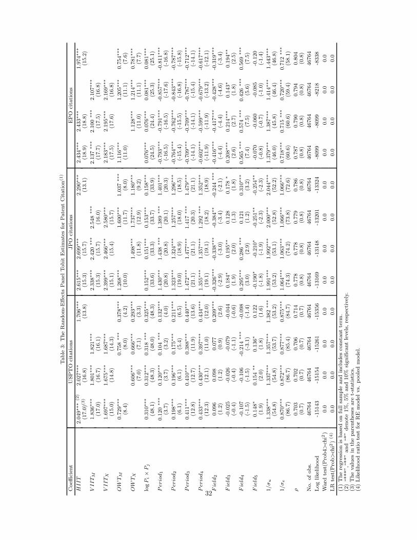
Table

3:

The

Random

-Effec

tsPanel

Tobit

Est

imate

sfo

rPate

nt

Cit

ati

on(1

)

Coeffi

cien

tU

SP

TO

cita

tions

JP

Oci

tati

ons

EP

Oci

tati

ons

HIIT

2.0

49∗∗

∗(2

)2.0

27∗∗

∗1.7

06∗∗

∗2.6

15∗∗

∗2.6

99∗∗

∗2.2

90∗∗

∗2.4

34∗∗

∗2.4

33∗∗

∗1.9

74∗∗

∗(1

7.0

)(3)

(16.8

)(1

3.8

)(1

5.3

)(1

5.7

)(1

3.1

)(1

8.9

)(1

8.8

)(1

5.2

)

VIIT

M1.8

36∗∗

∗1.8

01∗∗

∗1.8

21∗∗

∗2.3

38∗∗

∗2.4

20

∗∗∗

2.5

48

∗∗∗

2.1

37

∗∗∗

2.1

00

∗∗∗

2.1

07∗∗

∗(1

7.0

)(1

6.7

)(1

6.1

)(1

5.3

)(1

5.7

)(1

6.0

)(1

7.7

)(1

7.5

)(1

6.8

)

VIIT

X1.6

97∗∗

∗1.6

75∗∗

∗1.6

87∗∗

∗2.3

99∗∗

∗2.4

66∗∗

∗2.5

80∗∗

∗2.1

83∗∗

∗2.1

95∗∗

∗2.1

69∗∗

∗(1

5.0

)(1

4.8

)(1

4.3

)(1

5.1

)(1

5.4

)(1

5.7

)(1

7.5

)(1

7.6

)(1

6.8

)

OW

TM

0.7

29∗∗

∗0.7

58

∗∗∗

0.3

78∗∗

∗1.2

68∗∗

∗1.6

00∗∗

∗1.0

37

∗∗∗

1.1

16∗∗

∗1.2

05∗∗

∗0.7

54∗∗

∗(8

.4)

(8.0

)(4

.2)

(10.0

)(1

1.7

)(8

.0)

(11.0

)(1

1.1

)(7

.6)

OW

TX

0.6

06∗∗

∗0.6

66∗∗

∗0.2

93∗∗

∗1.4

98∗∗

∗1.7

37∗∗

∗1.1

80∗∗

∗1.1

28∗∗

∗1.2

14∗∗

∗0.7

81∗∗

∗(7

.0)

(7.1

)(3

.3)

(11.8

)(1

2.9

)(9

.2)

(11.0

)(1

1.1

)(7

.7)

log

Pi×

Pj

0.3

10∗∗

∗0.3

12∗∗

∗0.3

18

∗∗∗

0.3

25∗∗

∗0.1

52∗∗

∗0.1

51∗∗

∗0.1

53∗∗

∗0.1

58∗∗

∗0.0

76∗∗

∗0.0

76∗∗

∗0.0

81∗∗

∗0.0

81∗∗

∗(4

8.1

)(4

8.3

)(4

8.0

)(4

8.3

)(3

3.6

)(3

3.3

)(3

3.7

)(3

3.9

)(2

4.5

)(2

4.4

)(2

5.3

)(2

5.1

)

Per

iod1

0.1

20

∗∗∗

0.1

20∗∗

∗0.1

04

∗∗∗

0.1

32∗∗

∗1.4

30∗∗

∗1.4

38

∗∗∗

1.3

89

∗∗∗

1.4

01∗∗

∗-0

.793∗∗

∗-0

.791∗∗

∗-0

.857∗∗

∗-0

.811∗∗

∗(3

.7)

(3.7

)(3

.2)

(4.0

)(2

0.8

)(2

0.8

)(2

0.1

)(2

0.3

)(-

16.5

)(-

16.5

)(-

17.6

)(-

16.8

)

Per

iod2

0.1

98∗∗

∗0.1

96∗∗

∗0.1

75∗∗

∗0.2

11∗∗

∗1.3

23∗∗

∗1.3

24∗∗

∗1.2

57∗∗

∗1.2

96∗∗

∗-0

.764∗∗

∗-0

.762∗∗

∗-0

.843∗∗

∗-0

.787∗∗

∗(6

.1)

(6.1

)(5

.4)

(6.5

)(1

9.0

)(1

8.9

)(1

8.0

)(1

8.5

)(-

15.4

)(-

15.5

)(-

16.8

)(-

15.8

)

Per

iod3

0.4

11∗∗

∗0.4

10∗∗

∗0.3

88∗∗

∗0.4

40∗∗

∗1.4

72∗∗

∗1.4

77∗∗

∗1.4

17

∗∗∗

1.4

79∗∗

∗-0

.709∗∗

∗-0

.709∗∗

∗-0

.787∗∗

∗-0

.712∗∗

∗(1

2.8

)(1

2.7

)(1

1.9

)(1

3.6

)(2

1.1

)(2

1.1

)(2

0.3

)(2

1.1

)(-

14.1

)(-

14.1

)(-

15.4

)(-

14.1

)

Per

iod4

0.4

33∗∗

∗0.4

30∗∗

∗0.3

97∗∗

∗0.4

34∗∗

∗1.3

55∗∗

∗1.3

57∗∗

∗1.2

92

∗∗∗

1.3

52∗∗

∗-0

.602∗∗

∗-0

.599∗∗

∗-0

.679∗∗

∗-0

.617∗∗

∗(1

2.3

)(1

2.1

)(1

1.0

)(1

2.0

)(1

9.1

)(1

9.1

)(1

8.2

)(1

8.9

)(-

11.9

)(-

11.9

)(-

13.2

)(-

12.1

)

Fie

ld2

0.0

96

0.0

98

0.0

77

0.2

09∗∗

∗-0

.326∗∗

∗-0

.338∗∗

∗-0

.384∗∗

-0.2

44

∗∗∗

-0.4

16∗∗

∗-0

.417∗∗

∗-0

.428∗∗

∗-0

.319∗∗

∗(1

.2)

(1.2

)(0

.9)

(2.6

)(-

2.9

)(-

3.0

)(-

3.4

)(-

2.1

)(-

4.4

)(-

4.4

)(-

4.6

)(-

3.4

)

Fie

ld3

-0.0

25

-0.0

26

-0.0

79

-0.0

44

0.1

84∗

0.1

95∗∗

0.1

28

0.1

78

∗0.2

08∗∗

∗0.2

14∗∗

∗0.1

43∗

0.1

94∗∗

(-0.4

)(-

0.4

)(-

1.1

)(-

0.6

)(1

.9)

(2.0

)(1

.3)

(1.8

)(2

.6)

(2.7

)(1

.8)

(2.5

)

Fie

ld4

-0.1

07

-0.1

06

-0.2

14

∗∗∗

-0.0

98

0.2

95∗∗

∗0.2

86

∗∗∗

0.1

21

0.3

10∗∗

∗0.5

65

∗∗∗

0.5

74

∗∗∗

0.4

26

∗∗∗

0.5

69

∗∗∗

(-1.5

)(-

1.5

)(-

3.1

)(-

1.4

)(3

.0)

(2.9

)(1

.2)

(3.2

)(7

.4)

(7.5

)(5

.6)

(7.5

)

Fie

ld5

0.1

48∗

0.1

54

∗∗0.1

36∗

0.1

22

-0.1

90∗

-0.2

10∗

-0.2

51∗∗

-0.2

54∗∗

-0.0

70

-0.0

60

-0.0

85

-0.1

20

(1.9

)(2

.0)

(1.8

)(1

.6)

(-1.8

)(-

1.9

)(-

2.3

)(-

2.3

)(-

0.8

)(-

0.7

)(-

1.0

)(-

1.4

)

1/σ

u1.3

38∗∗

∗1.3

37∗∗

∗1.3

57∗∗

∗1.3

82

∗∗∗

1.9

91∗∗

∗1.9

92∗∗

∗2.0

00∗∗

∗2.0

44∗∗

∗1.3

79∗∗

∗1.3

87∗∗

∗1.4

14∗∗

∗1.4

43∗∗

∗(5

4.8

)(5

4.8

)(5

3.7

)(5

3.2

)(5

3.2

)(5

3.1

)(5

2.8

)(5

2.2

)(4

6.0

)(4

5.8

)(4

6.4

)(4

6.8

)

1/σ

e0.8

70∗∗

∗0.8

72∗∗

∗0.8

77∗∗

∗0.8

75∗∗

∗1.0

64∗∗

∗1.0

63∗∗

∗1.0

66∗∗

∗1.0

66∗∗

∗0.7

18∗∗

∗0.7

15

∗∗∗

0.7

20∗∗

∗0.7

12

∗∗∗

(86.7

)(8

6.7

)(8

5.4

)(8

4.7

)(7

4.3

)(7

4.2

)(7

3.8

)(7

2.6

)(6

0.6

)(6

0.6

)(5

9.4

)(5

8.1

)

ρ0.7

03

0.7

02

0.7

06

0.7

14

0.7

78

0.7

78

0.7

79

0.7

86

0.7

87

0.7

90

0.7

94

0.8

04

(0.7

)(0

.7)

(0.7

)(0

.7)

(0.8

)(0

.8)

(0.8

)(0

.8)

(0.8

)(0

.8)

(0.8

)(0

.8)

No.

ofobs.

46764

46764

46764

46764

46764

46764

46764

46764

46764

46764

46764

46764

Log

likel

ihood

-15143

-15154

-15261

-15356

-13169

-13148

-13201

-13324

-8099

-8099

-8218

-8338

Ward

test

(Pro

b4>

chi2

)0.0

0.0

0.0

0.0

0.0

0.0

0.0

0.0

0.0

0.0

0.0

0.0

LR

test

(Pro

b>

chi2

)(4

)0.0

0.0

0.0

0.0

0.0

0.0

0.0

0.0

0.0

0.0

0.0

0.0

(1)

The

regre

ssio

nis

base

don

full

sam

ple

and

incl

udes

const

ant

term

.(2

)“***”,“

**”

and

“*”

den

ote

1%

,5%

and

10%

signifi

cant

level

s,re

spec

tivel

y.(3

)T

he

valu

esin

the

pare

nth

eses

are

t-st

ati

stic

s.(4

)Lik

elih

ood

rati

ote

stfo

rR

Em

odel

vs.

poole

dm

odel

.

32

Table

4:

Fix

ed-e

ffec

tsN

egati

ve

Bin

om

ialE

stim

ate

sfo

rPate

nt

Cit

ati

on(1

)

Coeffi

cien

tU

SP

TO

cita

tions

JP

Oci

tati

ons

EP

Oci

tati

ons

HIIT

0.7

79∗∗

∗(2

)0.6

73∗∗

∗0.3

50∗∗

∗0.4

00∗∗

∗0.8

71∗∗

∗0.3

43∗∗

0.4

69∗∗

0.6

36∗∗

∗0.2

34

(7.7

)(3

)(6

.5)

(3.8

)(2

.6)

(5.8

)(2

.5)

(2.4

)(3

.2)

(1.4

)

VIIT

M0.5

10∗∗

∗0.4

00∗∗

∗0.1

11

0.1

30

0.6

09∗∗

∗0.2

35∗

0.2

95

0.4

59∗∗

0.2

19

(5.4

)(4

.2)

(1.2

)(0

.9)

(4.3

)(1

.7)

(1.5

)(2

.3)

(1.2

)

VIIT

X0.6

89∗∗

∗0.5

80∗∗

∗0.2

91∗∗

∗0.4

93∗∗

∗0.9

74∗∗

∗0.5

98∗∗

∗0.5

98∗∗

∗0.7

73∗∗

∗0.5

18∗∗

∗

(7.1

)(5

.9)

(2.9

)(3

.4)

(6.6

)(4

.1)

(3.0

)(3

.8)

(2.8

)

OW

TM

0.2

53∗∗

∗-0

.108

-0.1

47∗

-0.2

59∗

-0.1

10

-0.2

48∗

0.2

35

0.1

92

0.0

52

(2.7

)(-

1.1

)(-

1.7

)(-

1.8

)(-

0.8

)(-

1.8

)(1

.2)

(1.0

)(0

.3)

OW

TX

-0.0

38

-0.2

92∗∗

∗-0

.329∗∗

∗0.9

68∗∗

∗0.6

57∗∗

∗0.5

14

∗∗∗

0.6

08∗∗

∗0.4

07∗∗

0.2

64

(-0.4

)(-

3.1

)(-

3.8

)(7

.2)

(4.8

)(4

.1)

(3.1

)(2

.1)

(1.5

)

log

Pi×

Pj

0.2

52∗∗

∗0.2

51∗∗

∗0.2

56∗∗

∗0.2

57∗∗

∗0.0

58∗∗

∗0.0

56∗∗

∗0.0

58∗∗

∗0.0

58∗∗

∗0.0

24∗∗

∗0.0

24∗∗

∗0.0

24∗∗

∗0.0

23∗∗

∗

(27.7

)(2

7.4

)(2

7.8

)(2

8.1

)(1

2.2

)(1

1.8

)(1

2.1

)(1

2.2

)(6

.5)

(6.5

)(6

.6)

(6.5

)

Per

iod1

0.1

93∗∗

∗0.1

94∗∗

∗0.1

93∗∗

∗0.1

98∗∗

∗2.3

73∗∗

∗2.4

02∗∗

∗2.3

70∗∗

∗2.3

74∗∗

∗-0

.181∗∗

∗-0

.183

∗∗∗

-0.1

88∗∗

∗-0

.172∗∗

∗

(6.8

)(6

.8)

(6.7

)(6

.9)

(31.0

)(3

1.3

)(3

0.9

)(3

0.9

)(-

3.2

)(-

3.2

)(-

3.3

)(-

3.0

)

Per

iod2

0.4

09

0.4

12

0.4

15

0.4

17

2.3

85

2.4

06

2.3

78

2.3

82

-0.0

39

-0.0

47

-0.0

48

-0.0

32

(14.9

)(1

5.0

)(1

5.0

)(1

5.1

)(3

0.8

)(3

1.0

)(3

0.6

)(3

0.7

)(-

0.7

)(-

0.8

)(-

0.8

)(-

0.6

)

Per

iod3

0.7

26∗∗

∗0.7

30∗∗

∗0.7

33∗∗

∗0.7

36∗∗

∗2.5

67∗∗

∗2.5

81∗∗

∗2.5

64∗∗

∗2.5

70∗∗

∗0.1

19∗∗

0.1

13∗

0.1

19∗∗

0.1

38

∗∗

(26.1

)(2

6.2

)(2

6.0

)(2

6.2

)(3

3.2

)(3

3.3

)(3

3.0

)(3

3.2

)(2

.0)

(1.9

)(2

.0)

(2.3

)

Per

iod4

1.0

19∗∗

∗1.0

25∗∗

∗1.0

29∗∗

∗1.0

26∗∗

∗2.6

08∗∗

∗2.6

18∗∗

∗2.6

02∗∗

∗2.6

07∗∗

∗0.3

18∗∗

∗0.3

07∗∗

∗0.3

13∗∗

∗0.3

29∗∗

∗

(29.6

)(2

9.8

)(2

9.4

)(2

9.4

)(3

3.3

)(3

3.4

)(3

3.2

)(3

3.3

)(5

.4)

(5.2

)(5

.3)

(5.6

)

No.

ofobs.

11874

11874

11874

11874

8900

8900

8900

8900

6110

6110

6110

6110

Log

likel

ihood

-15538

-15542

-15562

-15559

-11335

-11311

-11327

-11332

-6216

-6212

-6217

-6220

Ward

test

(Pro

b4>

chi2

)0.0

0.0

0.0

0.0

0.0

0.0

0.0

0.0

0.0

0.0

0.0

0.0

(1)

The

regre

ssio

nis

base

don

full

sam

ple

.

(2)

“***”,“

**”

and

“*”

den

ote

1%

,5%

and

10%

signifi

cant

level

s,re

spec

tivel

y.

(3)

The

valu

esin

the

pare

nth

eses

are

t-st

ati

stic

s.

33

Table A.1: Descriptive Statistics

Variable No. of Obs Mean StdDev Min MaxHIIT 46764 0.05 0.10 0.00 1.00V IIT 46764 0.17 0.19 0.00 1.00OWT 46764 0.28 0.24 0.00 1.00

USPTO citations 47300 14.9 400.0 0 56342Pi in USPTO 47300 412.0 2803.6 0 59160Pj in USPTO 47300 412.0 2803.6 0 59160JPO citations 47300 14.5 419.0 0 39332

Pi in JPO 47300 2382.7 19395.3 0 279823Pj in JPO 47300 1527.8 11114.7 0 233511

EPO citations 47300 0.9 18.3 0 1614Pi in EPO 47300 275.1 1273.5 0 16533Pj in EPO 47300 275.1 1273.5 0 16533

34

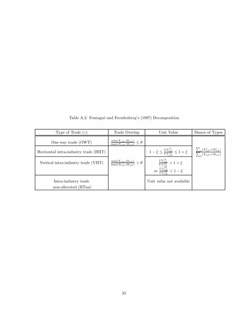
Table A.2: Fontagne and Freudenberg’s (1997) Decomposition

Type of Trade (z) Trade Overlap Unit Value Shares of Types

One-way trade (OWT) min(Xijk ,Mijk)max(Xijk,Mijk) ≤ θ

Horizontal intra-industry trade (HIIT) 1 − ξ ≤ UV Xijk

UV Mijk

≤ 1 + ξ

∑k(Xz

ijk+Mzijk)∑

k(Xijk+Mijk)

Vertical intra-industry trade (VIIT) min(Xijk ,Mijk)max(Xijk,Mijk) > θ

UV Xijk

UV Mijk

> 1 + ξ

orUV X

ijk

UV Mijk

< 1 − ξ

Intra-industry trade Unit value not availablenon-allocated (IITna)

35

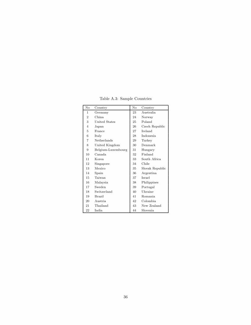
Table A.3: Sample Countries

No Country No Country

1 Germany 23 Australia

2 China 24 Norway

3 United States 25 Poland

4 Japan 26 Czech Republic

5 France 27 Ireland

6 Italy 28 Indonesia

7 Netherlands 29 Turkey

8 United Kingdom 30 Denmark

9 Belgium-Luxembourg 31 Hungary

10 Canada 32 Finland

11 Korea 33 South Africa

12 Singapore 34 Chile

13 Mexico 35 Slovak Republic

14 Spain 36 Argentina

15 Taiwan 37 Israel

16 Malaysia 38 Philippines

17 Sweden 39 Portugal

18 Switzerland 40 Ukraine

19 Brazil 41 Romania

20 Austria 42 Colombia

21 Thailand 43 New Zealand

22 India 44 Slovenia

36

Table A.4: Correspondence derived by Schmoch et al. between technical fields and ISIC industrialclassifications1

Field No. Sector ISIC ver. 3

1 food 15

2 tobacco 16

3 textiles 17

4 wearing 18

5 leather 19

6 wood products 20

7 paper 21

8 publishing 22

9 petroleum 23

10 basic chemicals 241

11 pesticides 2421

12 paint 2422

13 pharmaceuticals 2423

14 soaps 2424

15 other chemicals 2429

16 man-made fibres 243

17 plastic products 25

18 mineral products 26

19 basic metals 27

20 metal products 28

21 energy machinery 2911, 2912, 2913

22 non-specific machinery 2914, 2915, 2919

23 agricultural machinery 2921

24 machine-tools 2922

25 special machinery 2923, 2924, 2925, 2926, 2929

26 weapons 2927

27 domestic appliances 293

28 computers 30

29 electrical motors 311

30 electrical distribution 312, 313

31 accumulators 314

32 lightening 314

33 other electrical 315

34 electronic components 321

35 telecommunications 322

36 television 323

37 medical equipment 3311

38 measuring instruments 3312

39 industrial control 3313

40 optics 332

41 watches 333

42 motor vehicles 34

43 other transport 35

44 consumer goods 361Tables 3-1 and 3-5 in Schmoch et al. (2003).

37