TMD DISCUSSION PAPER NO. 93

TRADE AND TRADABILITY: EXPORTS, IMPORTS, ANDFACTOR MARKETS IN THE SALTER-SWAN MODEL

Karen ThierfelderU.S. Naval Academy and International Food Policy Research

Institute (IFPRI)and

Sherman RobinsonInternational Food Policy Research Insitute (IFPRI)

Trade and Macroeconomics DivisionInternational Food Policy Research Institute

2033 K Street, N.W.Washington, D.C. 20006, U.S.A.

May 2002

TMD Discussion Papers contain preliminary material and research results, and are circulated prior toa full peer review in order to stimulate discussion and critical comment. It is expected that most DiscussionPapers will eventually be published in some other form, and that their content may also be revised. This paper isavailable at http://www.cgiar.org/ifpri/divs/tmd/dp.htm

Abstract

We extend the Salter-Swan model to include both factor markets and semi-traded

goods. In our model, changes in relative factor prices depend on changes in world

commodity prices, factor endowments, and the trade balance. In contrast, only changes in

world commodity prices can affect factor prices in the neoclassical trade model. The

inclusion of semi-traded goods weakens the magnification effect of both the Stolper-

Samuelson and Rybczynski theorems. When imports and domestic goods are poor

substitutes, a characteristic of some commodities in developing countries, the sign of the

Stolper-Samuelson effect is reversed.

Key words: Semi-traded goods, two-way trade, Salter-Swan Model, Stolper-SamuelsonTheoremJEL codes: F11, F13, F15

We would like to thank Eugenio Diaz-Bonilla, Victoria Greenfield, Kenneth Hanson, Ronald Jones,*

Edward Leamer, Scott McDonald, J. David Richardson, Alasdair Smith, and Adrian Wood for helpfulrevisions to an earlier version of this paper.

Table of Contents

I. Introduction . . . . . . . . . . . . . . . . . . . . . . . . . . . . . . . . . . . . . . . . . . . . . . . . . . . . . . . . 1

II. The 1-2-2-3 Model . . . . . . . . . . . . . . . . . . . . . . . . . . . . . . . . . . . . . . . . . . . . . . . . . 2

III. Implications of Tradability for the Stolper-Samuelson Theorem . . . . . . . . . . . . . . . 11

IV. Implications of Tradability for the Rybczynski Theorem . . . . . . . . . . . . . . . . . . . . . 13

V. Trade Balance Effects . . . . . . . . . . . . . . . . . . . . . . . . . . . . . . . . . . . . . . . . . . . . . . . 14

VI. Conclusions . . . . . . . . . . . . . . . . . . . . . . . . . . . . . . . . . . . . . . . . . . . . . . . . . . . . . 16

References . . . . . . . . . . . . . . . . . . . . . . . . . . . . . . . . . . . . . . . . . . . . . . . . . . . . . . . . . . 19

Appendix . . . . . . . . . . . . . . . . . . . . . . . . . . . . . . . . . . . . . . . . . . . . . . . . . . . . . . . . . . . 22

Derivation of the wage decomposition equation in the 1-2-2-3 model . . . . . . . . . . . . . 23

List of Discussion Papers . . . . . . . . . . . . . . . . . . . . . . . . . . . . . . . . . . . . . . . . . . . . . . . 31

Armington (1969) used this specification in estimating import demand functions. Many empirical studies1

support this specification. For example, Shiells and Reinert (1993) find low import substitution elasticities for theU.S., Canada, and Mexico, suggesting that it is important to characterize imported and domestic goods as semi-tradable.

Many surveys of CGE trade models are available: NAFTA (Francois and Shiells, 1994), regional trade2

agreements and agriculture (Burfisher and Jones, 1998), and the Uruguay Round (Martin and Winters, 1996,Shoven and Whalley, 1992). Robinson (1989) and de Melo (1988) describe the application of these models todevelopment issues.

1

I. Introduction

In trade data, there is evidence of cross-hauling–countries import and export the same

commodity, even for the most detailed commodity categories. This observation is

inconsistent with neoclassical trade theory, in which goods are homogenous. According to

the Heckscher-Ohlin Samuelson (HOS) model, a country imports its non-comparative

advantage good and exports its comparative advantage good. There is no two-way trade at

the commodity level.

Empirical trade models account for cross-hauling by using the Armington (1969)

assumption that imports and domestic goods are imperfect substitutes in consumption.1

There is a large class of single- and multi-country, applied, computable general equilibrium

(CGE) trade models which incorporate the Armington assumption at the commodity level

to accommodate observed trade patterns. CGE models have been used extensively to analyze

the effect of free trade agreements as well as trade and domestic policy reform issues in both

developed and developing countries. 2

In this paper, we describe the theoretical properties of such trade models, focusing

on factor markets. We extend the Salter-Swan model, in which there is both a traded and a

non-traded good, and specify that imports and domestic good are imperfect substitutes in

This model was first described in Salter (1959) and Swan (1960).3

Abrego and Whalley (2000) and Krugman (2000) use a stylized model to analyze changes in factor prices. 4

They do not solve the model for an explicit decomposition equation, but rather use the model to simulate observedchanges in factor prices and commodity prices.

2

consumption. Rather than having a non-traded good, we have a semi-traded good. Similarly,3

exports and the domestic good are imperfect substitutes in production. As in the Salter-Swan

model, we include both domestic and traded goods so the model includes the real exchange

rate. We also draw upon Jones (1965) which includes factors, but not non-traded goods, and

Jones (1974) which includes a non-traded good, but not factor markets. We incorporate both

factor markets and semi-traded goods. In the extreme case, when imports and domestic goods

are perfect substitutes, our model collapses to the neoclassical HOS model.

The Stolper-Samuelson and Rybczynski theorems describe the links between trade

and factor markets. We show how these theorems operate in a model with semi-traded goods.

We find that the magnification effect of both theorems is weaker. Furthermore, when

imports and domestic goods are poor substitutes in consumption, a characteristic of some

commodities in developing countries, the sign of the Stolper-Samuelson effect is reversed.

We also provide a decomposition equation showing the effects of changes in relative

commodity prices, changes in the relative endowment, and changes in the trade balance on

changes in relative factor prices.4

II. The 1-2-2-3 Model

Our analytical model closely follows Jones (1974) who incorporates a non-traded

good into the 2x2x2 HOS framework. We expand Jones (1974) by (1) exploring the

factor market linkages, which he did not include in the model with a non-traded good; (2)

Q ' F (M,D ;σQ )

MD

' k P D

P M

σQ

σQ

Devarajan, Lewis, and Robinson (1990, 1993) explore the properties of the model in detail, extending it to5

include tariffs and taxes, and also use the same basic framework to analyze issues concerning the appropriatedefinition of the equilibrium real exchange rate.

3

(1)

(2)

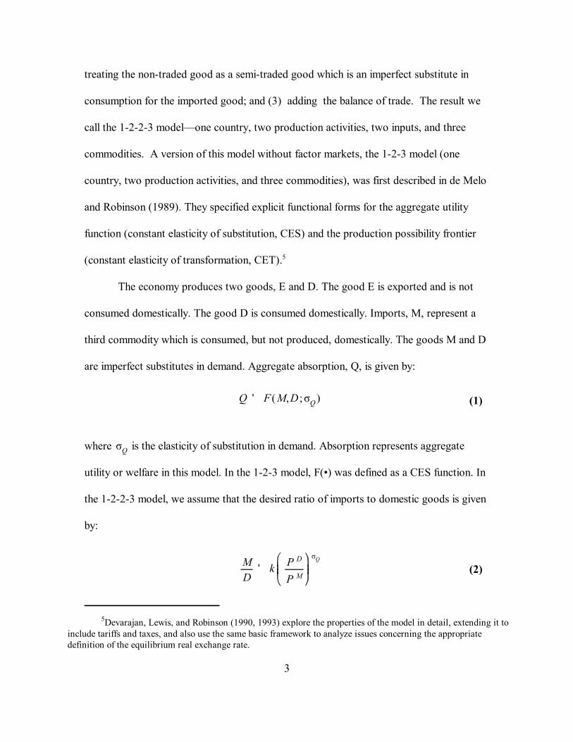
treating the non-traded good as a semi-traded good which is an imperfect substitute in

consumption for the imported good; and (3) adding the balance of trade. The result we

call the 1-2-2-3 model—one country, two production activities, two inputs, and three

commodities. A version of this model without factor markets, the 1-2-3 model (one

country, two production activities, and three commodities), was first described in de Melo

and Robinson (1989). They specified explicit functional forms for the aggregate utility

function (constant elasticity of substitution, CES) and the production possibility frontier

(constant elasticity of transformation, CET).5

The economy produces two goods, E and D. The good E is exported and is not

consumed domestically. The good D is consumed domestically. Imports, M, represent a

third commodity which is consumed, but not produced, domestically. The goods M and D

are imperfect substitutes in demand. Aggregate absorption, Q, is given by:

where is the elasticity of substitution in demand. Absorption represents aggregate

utility or welfare in this model. In the 1-2-3 model, F(•) was defined as a CES function. In

the 1-2-2-3 model, we assume that the desired ratio of imports to domestic goods is given

by:

A '

AKE AKD

ALE ALD

AKE E % AKD D ' K

ALE E % ALD D ' L

AKE WK % ALE WL ' P E

AKD WK % ALD WL ' P D

In the general case, we ignore income effects and assume the absorption function is well behaved (e.g.6

homothetic, convex, and twice-differentiable).

We also assume that both sectors use both factors in equilibrium, so there are no corner solutions. 7

4

(3)

(4)

(5)

where k is constant for a CES function and approximately constant otherwise, and P andM

P are the prices of M and D respectively. D 6

Following Jones’ notation, the technology for producing E and D is given by the

coefficients matrix A:

where A is the quantity of factor i required to produce a unit of good j. We do notij

assume that these coefficients are constant. When the coefficients are variables, however,

they are assumed to depend only on relative factor prices —there is no technical change.7

Given this technology, factor market clearing requires:

where K and L are aggregate supplies of capital and labor.

In competitive equilibrium, unit costs will equal market prices:

P M M ' Φ P E E

5

(6)

where W and W are the “wages” of capital and labor and P and P are output prices. K LE D

To close this model, we require an equation linking exports and imports. We assume that

the balance of trade is given by:

where Φ is a parameter giving the ratio of import expenditures to export earnings. This

specification extends the standard HOS model, allowing the balance of trade to affect

consumption, production, and factor returns. When Φ is one, trade is balanced, with

export earnings exactly equaling import costs —as in the usual HOS model. The trade

balance (the value of exports minus imports in world prices) equals (1 - Φ) times export

earnings. An increase in Φ implies a worsening of the trade balance.

Assuming that the country is “small” so that we can assume world prices, P andM

P , are fixed, the model is complete. There are seven equations for seven endogenousE

variables: Q, E, D, M, W , W , and P . Unlike the HOS model, one of the commodityK LD

prices is endogenous.

We demonstrate how the endogenous variables, particularly relative wages,

change in response to changes in the prices of the traded goods (P and P ), factorE M

supplies (K and L), and the balance of trade (Φ). First, we define the share parameters and

elasticities that are important to the linkages. Our notation again follows Jones (1965).

Define λ as the share of the total supply of factor i used in sector j:ij

λKE 'AKE E

K; λKD '

AKD DK

λLE 'ALE E

L; λLD '

ALD DL

θij 'Aij Wi

P j

jjλi j ' j

iθi j ' 1

λ '

λKE λKD

λLE λLD

θ '

θKE θLE

θKD θLD

θKE > θKD

λKE > λLE

6

(7)

(8)

(9)

(10)

(11)

Define θ as the share of factor i in total income generated in sector j. ij

Given that factors are fully employed and that income is fully allocated to factors (zero

profit condition), it follows that:

We will assume that E is the capital-intensive sector and that D is labor-intensive.

Capital’s value share in E must be greater than its value share in D, ( ), and

also the share of the total capital stock used in E must be greater than the share of the

labor force used in E, ( ). Define the following matrices:

λ ' λKE & λLE ; θ ' θKE & θKD

σE 'ALE & AKE

WK & WL

σD 'ALD & AKD

WK & WL

δK ' λKE θLE σE % λKD θLD σD

δL ' λLE θKE σE % λLD θKD σD

7

(12)

(13)

(14)

Given that the rows of each of these matrices sum to one, their determinants are given by:

Under the assumption that E is capital intensive, both determinants are positive (and less

than one).

Use a (ˆ) to denote the relative change in a variable or parameter (or its log

derivative). The elasticities of substitution between capital and labor in production in the

two sectors E and D can be defined by:

In addition, define two additional parameters:

Quoting Jones (1965, p. 35): “In general, δ is the aggregate percentage saving in laborL

inputs at unchanged outputs associated with a 1% rise in the relative wage rate, the saving

resulting from the adjustment to less labor-intensive techniques in both industries as

relative wages rise.”

Ω 'δK % δL

λ θ

WK & WL '1θ

P E& P D

θ < 1

It is well known that the transformation elasticity is close to linear when technology is either Cobb-8

Douglas or CES (with high elasticities), as shown in Johnson (1966). See also Abrego and Whalley (2000) for amore recent discussion.

Details of the derivations are given in Robinson and Thierfelder (1996). 9

8

(15)

(16)

Finally, the elasticity of transformation between E and D (along the production

possibility frontier) is given by:

In the original 1-2-3 model, the production possibility frontier was defined as a CET

function, with a constant Ω. In the 1-2-2-3 model, we only assume it to be approximately

fixed when taking log derivatives. 8

The model reduces to four relationships in changes in relative prices, production,

and demand. The first is the link between changes in relative prices and relative wages9

along the contract curve underlying the production possibility frontier.

In the standard HOS model, where both goods are tradeable and their prices are set in

world markets, this equation demonstrates the Stolper-Samuelson Theorem. Relative

wages depend only on relative prices and, since , the change in relative wages is

greater than the change in relative prices—the model incorporates the magnification

effect.

E & D '1λ

K & L % Ω P E& P D

M & D ' &σQ P M& P D

E & M ' P M& P E

& Φ

λ < 1

Equations 16 and 17 present results for relative wages and production. When only one price changes, one10

can show that one wage goes up while the other falls (Stolper-Samuelson). Similarly, one can show that, with achange in one factor endowment, one output goes up while the other falls (Rybczynski).

9

(17)

(18)

(19)

Second, movements along the production possibility frontier are determined both

by changes in relative prices and changes in relative factor endowments.

This equation demonstrates the Rybczynski Theorem. Since , with unchanged

prices, changes in relative factor endowments will have a magnified effect on relative

production. 10

The demand side of the model involves D and M rather than D and E. Log differentiating

equation 2 yields:

This equation shows how relative demand for M and D changes with changes in relative

prices.

Finally, the supply and demand sides are linked through the balance-of-trade equation.

Log differentiating equation 6 yields:

The changes in relative prices of D and E can be expressed as a function of changes in

exogenous world prices, factor endowments, and the balance of trade:

P E& P D

'1

σQ % Ω(σQ & 1) (P E

& P M ) & Φ %1λ

L & K

WK & WL '1

θ σQ % Ω(σQ & 1) (P E

& P M ) & Φ %1λ

L & K

P D

This equation is equivalent to the equation for the equilibrium real exchange rate in the 1-2-3 model11

derived in Devarajan, Lewis, and Robinson (1993), with the addition of a term for changes in factor endowments.

10

(20)

(21)

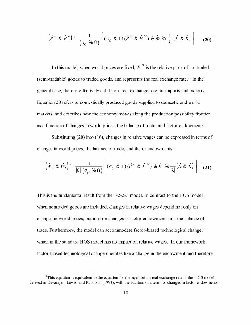
In this model, when world prices are fixed, is the relative price of nontraded

(semi-tradable) goods to traded goods, and represents the real exchange rate. In the11

general case, there is effectively a different real exchange rate for imports and exports.

Equation 20 refers to domestically produced goods supplied to domestic and world

markets, and describes how the economy moves along the production possibility frontier

as a function of changes in world prices, the balance of trade, and factor endowments.

Substituting (20) into (16), changes in relative wages can be expressed in terms of

changes in world prices, the balance of trade, and factor endowments:

This is the fundamental result from the 1-2-2-3 model. In contrast to the HOS model,

when nontraded goods are included, changes in relative wages depend not only on

changes in world prices, but also on changes in factor endowments and the balance of

trade. Furthermore, the model can accommodate factor-biased technological change,

which in the standard HOS model has no impact on relative wages. In our framework,

factor-biased technological change operates like a change in the endowment and therefore

WK & WL '1θ

P E& P M

WK & WL '1θ

σQ & 1σQ % Ω

(P E& P M )

σQ

P D' P M

11

(22)

(23)

affects relative wages.

III. Implications of Tradability for the Stolper-Samuelson Theorem

As the elasticity of substitution in consumption, , goes to infinity, the last two

terms in brackets in equation 21 go to zero. In the limit, the remaining term in world

prices reduces to:

which corresponds to equation 16 with since D and M are now perfect

substitutes. This is exactly the HOS model, with changes in relative wages depending

only on changes in world prices, and the Stolper-Samuelson Theorem again applies. The

HOS model can thus be seen as a special case of the 1-2-2-3 model when imports and

domestic goods are perfect substitutes.

When there is no change in factor supplies and the balance of trade, equation 21

reduces to:

Since Ω is positive, the second term in this expression is always less than one. The result

is that the magnification effect in the Stolper-Samuelson Theorem is reduced. The larger

is the transformation elasticity Ω and the closer is the elasticity of substitution in demand

to one, the weaker is the link between changes in prices and changes in relative wages.

When the elasticity of substitution equals one, the right-hand side goes to zero and

σQ ' 1

σQ > 1

σQ < 1

The model is characterized by Lerner symmetry. It does not matter whether world export or import prices12

change. In the cases discussed below, for expositional convenience, we will start from a change in the world priceof imports, assuming export prices are fixed.

Bhattarai, Ghosh, and Whalley (1999) assert that when the Armington elasticity is less than one, a13

country’s offer curve is “perverse.” We would argue that they are not perverse, but rather describe commoditiessuch as capital goods, for which imports are poor substitutes for the domestic good in developing countries. Allstandard trade theory texts show the offer curves as having an upward sloping, a vertical, and a backward bending

12

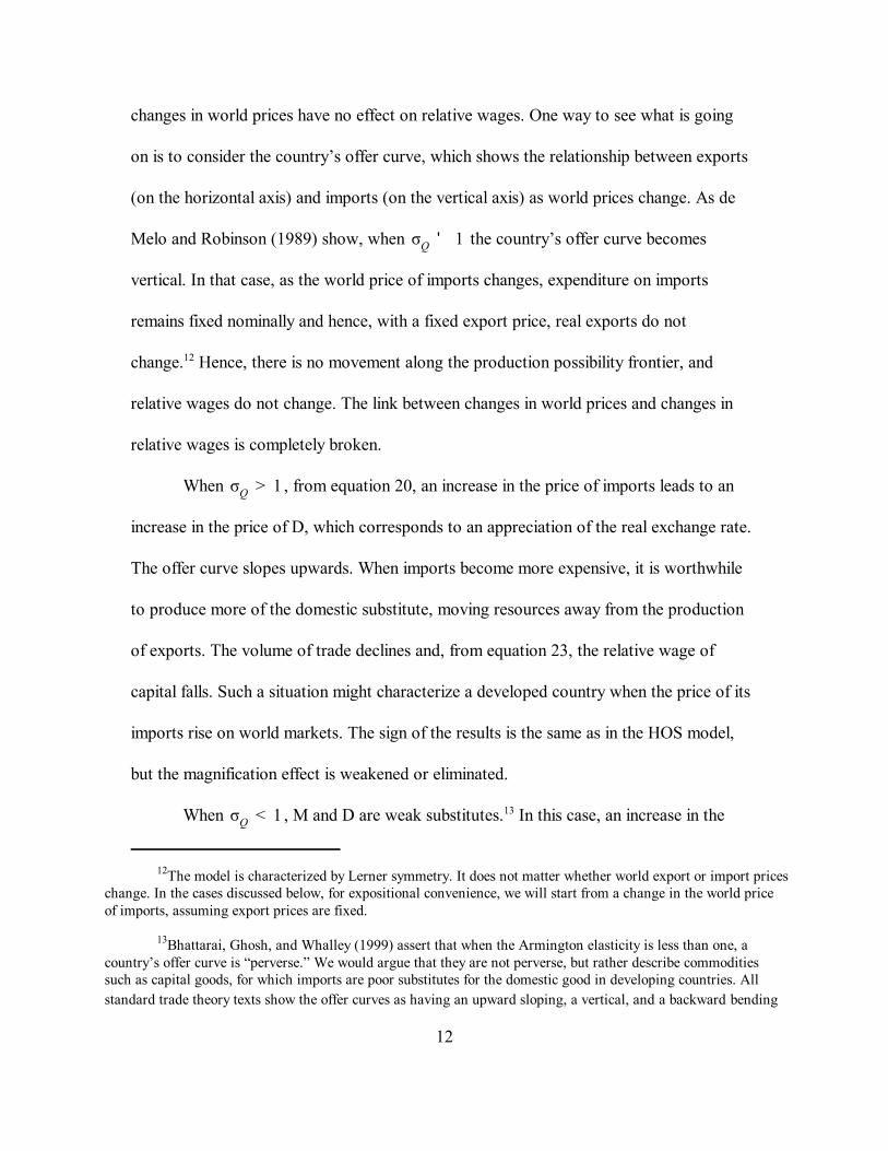
changes in world prices have no effect on relative wages. One way to see what is going

on is to consider the country’s offer curve, which shows the relationship between exports

(on the horizontal axis) and imports (on the vertical axis) as world prices change. As de

Melo and Robinson (1989) show, when the country’s offer curve becomes

vertical. In that case, as the world price of imports changes, expenditure on imports

remains fixed nominally and hence, with a fixed export price, real exports do not

change. Hence, there is no movement along the production possibility frontier, and12

relative wages do not change. The link between changes in world prices and changes in

relative wages is completely broken.

When , from equation 20, an increase in the price of imports leads to an

increase in the price of D, which corresponds to an appreciation of the real exchange rate.

The offer curve slopes upwards. When imports become more expensive, it is worthwhile

to produce more of the domestic substitute, moving resources away from the production

of exports. The volume of trade declines and, from equation 23, the relative wage of

capital falls. Such a situation might characterize a developed country when the price of its

imports rise on world markets. The sign of the results is the same as in the HOS model,

but the magnification effect is weakened or eliminated.

When , M and D are weak substitutes. In this case, an increase in the13

θ < 0

P E& P D

segment.

13

world price of M leads to a decrease in the price of D relative to E, which is a

depreciation of the real exchange rate. Production of D declines and exports increase. In

effect, the country depreciates in order to shift resources into exports, increasing export

earnings in order to pay for the more expensive, but essential, imports. The offer curve is

backward bending. This situation is characteristic of developing countries which have to

undergo a structural adjustment program in the face of an adverse terms-of-trade shock

(for example, a large increase in the price of oil). In this case, changing a commodity

price has the opposite effect on wages than would be predicted by the HOS model. In a

developing country exporting labor-intensive goods, where , an increase in the

price of imports will lead to an increase in the wage of labor relative to capital, while the

HOS model would predict a decrease. The 1-2-2-3 model seems much more realistic in

this case.

IV. Implications of Tradability for the Rybczynski Theorem

To consider the application of the Rybczynski Theorem in the 1-2-2-3 model,

consider the relationship between the change in domestic relative prices as factor

endowments change when world prices and the balance of trade do not change (equation

20). Substitute the resulting expression for into equation 17. The result is an

expression relating the change in the structure of production as a function of the change in

factor endowments, all other exogenous variables held constant:

E & D '1λ

σQ

σQ % ΩK & L

σQ

σQ

σQ < 1

14

(24)

As with the Stolper-Samuelson Theorem, this equation reduces to the HOS

version (equation 17, the Rybczynski Theorem) as a special case in the limit when the

elasticity of substitution ( ) goes to infinity. In general, however, the magnification

effect in the Rybczynski Theorem is ameliorated. Since Ω is greater than zero, the term in

brackets is less than one. The greater is Ω and the lower is , the weaker is the link

between changes in factor endowments and changes in the structure of production. Unlike

the Stolper-Samuelson Theorem, there is no sign reversal when .

V. Trade Balance Effects

One view of the effect of changes in the balance of trade on relative wages is that

a worsening in the trade balance (increasing Φ) leads to increased imports which displace

domestic production of low-skill, labor-intensive goods (D), and hence should widen the

wage gap. Borjas, Freeman, and Katz (1992), using the factor-content approach, compute

the net implicit contribution of the trade deficit to the supply of labor by different skill

categories. They conclude (p. 214): “The annual increase in implicit labor supply due to

the mid- and late-1980s trade deficit in manufactures was on the order of 1.5 percent for

the economy as a whole and 6 percent for the manufacturing sector.” They then analyze

the impact of these shifts on wages in a partial-equilibrium analysis of the labor markets,

concluding that “. . . from 15 to 25 percent of the 11 percentage point rise in the earnings

of college graduates relative to high school graduates from 1980 to 1985 can be attributed

Φ

The Dutch disease occurs when an increase in availability of foreign exchange (arising, say, from the dis-14

covery of oil in the North Sea) worsens the trade balance and generates a real appreciation of the exchange rate,increasing imports, and reducing production of tradables.

Bhagwati and Dehejia (1994) also criticize Borjas, Freeman, and Katz, but from the perspective of the15

HOS model, arguing that changes in endowments should have no effect on relative wages. Leamer (1996, pp. 11-12) considers a model with nontradables and notes that: “An external deficit raises the demand for nontradablesand may or may not affect wages.” In a footnote, he worries about different causes of a change in the deficit, andhow they might affect relative wages.

15

to the massive increase in the trade deficit over the same period.”

In equation 21, however, an increase in Φ will lead to a narrowing of the wage

gap, since the sign of the coefficient on is negative. There is a serious conflict between

the 1-2-2-3 model and the labor-market approach. The problem is a conflict between

partial- and general-equilibrium models. The labor-market approach assumes that

increased imports due to the worsening of the balance of trade will “displace” domestic

production of labor-intensive goods. However, increasing Φ implies that absorption will

rise since the worsening trade balance shifts the consumption possibility frontier out, even

though the production possibility frontier stays the same. Consumers have more to spend

and, since D is a normal good, they will demand more D as well as more M. The effect

will be to increase the relative price of D, as shown in equation 20, shifting resources

away from E to produce more D. The increase in P represents an appreciation of the realD

exchange rate and the model demonstrates the Dutch disease. The production of E14

declines, D expands, and the relative wage gap narrows. 15

VI. Conclusions

We extend the Salter-Swan and Jones models to include semi-tradable goods,

rather than a pure non-traded good, and also explicitly include factor markets. In this

Recent studies include Wood (1994), Sachs and Shatz (1994), and Borjas, Freeman, and Katz (1992,16

1996).

16

model, we show that the change in relative factor prices depends not only on changes in

commodity prices, as explained in the Stolper-Samuelson theorem, but also on changes in

factor endowments and in the balance of trade. We find that imperfect substitutability

between the import and domestic goods dampens the magnification effects in the Stolper-

Samuelson and Rybczynski theorems. When imports and domestic goods are poor

substitutes, the sign of the Stolper-Samuelson result is opposite of what the neoclassical

trade model predicts. We also find that the trade balance effect on relative factor returns

is the opposite of what factor content studies predict. In a general equilibrium

framework, we capture the absorption effect of a deterioration of the trade balance, as

well as the changes in the structure of production. Factor content analysis, using a partial

equilibrium framework, only accounts for the latter effect.

There are a number of implications for policy analysis of including semi-traded

goods in the model. For example, empirical models based on the 1-2-2-3 model can

provide a unifying framework for the trade-wage debate, in which labor and trade

economists have different approaches to explain the widening gap between skilled and

unskilled wages in developed countries observed in the 1980s. Labor economists

generally use partial equilibrium models measuring the factor content of traded goods. 16

Imports displace domestic production and, in effect, shift the demand for labor. Trade

economists, using the Heckscher-Ohlin-Samuelson (HOS) model, look for links between

See Leamer (1998), Baldwin and Cain (2000), and Harrigan and Baliban (1999) for regression analysis17

of trade relationships derived from a general equilibrium trade model. Slaughter (2000) provides an overview ofsuch commodity price studies.

For a discussion of the role of technological progress in the trade-wage debate, see Krugman (2000),18

Baldwin and Cain (2000), Leamer (1998), Francois and Nelson (1998) and Wood (1998).

17

commodity prices and factor prices. The 1-2-2-3 model can accommodate both trade17

balance and world price shocks.

The 1-2-2-3 also can be used to evaluate the effects of technological progress on

factor returns, another aspect of the trade-wage debate. According to the HOS model,18

only sector-biased technological progress can affect wages. As Richardson (1995, p. 42)

notes,

“The [trade-wage] debate increasingly and properly isolates trade prices

and sectoral total factor productivity differences as the causes of long-run

factor-price movements. Trade volumes are correspondingly treated

endogenously. Neutral and factor-augmenting technological change is seen

to be just like factor-supply change, with innocuous impacts on factor

prices.”

Other economists, notably Wood (1994, 1995, 1998), argue that trade can have a big

effect on wages when it induces factor-biased technological change. According to Wood,

imports of unskilled-labor-intensive goods from developing countries induce “defensive

innovation” by firms in developed countries as they use new production methods that

economize on unskilled labor. The 1-2-2-3 model can accommodate both types of

technological change. Factor-biased technological change will affect the wage gap

because it operates like an endowment change, which does affect wages in the 1-2-2-3

18

model.

Finally, a model with semi-traded goods and factor markets is important for

analysis of structural adjustment programs in developing countries. When imports and the

domestic good are poor substitutes, as is the case for many commodities that developing

countries import, a commodity price shock will have the opposite effect on factor returns

than that predicted using a neoclassical trade model. This linkage matters for poverty

analysis which looks at the effects of prices shocks on income.

19

References

Abrego, Lisandro and John Whalley (2000). “The Choice of Structural Model in Trade-Wage Decompositions,” Review of International Economics, Vol. 8 no. 3, pp.462-477.

Armington, Paul S. (1969). “A Theory of Demand for Products Distinguished by Place ofProduction.” IMF Staff Papers, Vol. 16, pp. 159-178.

Baldwin, Robert E. and Glen Cain (2000). “Shifts in Relative U.S. Wages: The Role ofTrade, Technology and Factor Endowments,” Review of Economics and Statistics,Vol. 82, no. 4, pp. 580-595.

Bhagwati, Jagdish and Vivek H. Dehejia (1994). “Freer Trade and Wages of theUnskilled —Is Marx Striking Again?” In Bhagwati and Kosters, editors, Tradeand Wages, Washington, D.C.: American Enterprise Institute.

Bhatarai, Keshab, Madanmohan Ghost, and John Whalley (1999). “More on TradeClosure.” In Gustav Ranis and Lakshmi K. Raut, editors, Trade Growth andDevelopment, Essays in Honor of Professor T.N. Srinivasan. New York: ElsevierPress.

Borjas, George J., Richard B. Freeman, and Lawrence F. Katz (1996). “Searching for theEffect of Immigration on the Labor Market.” Unpublished, Harvard Universityand NBER, presented to the American Economic Association Meetings, January5-7, 1996, San Francisco, California.

Borjas, George J,. Richard B. Freeman, and Lawrence F. Katz (1992). “On the LaborMarket Effects of Immigration and Trade” In G. Borjas and R. Freeman, eds.,Immigration and the Work Force. Chicago: University of Chicago and NBER, pp.245-69.

Burfisher, Mary E. and Elizabeth A. Jones, eds. (1998). Regional Trade Agreements andU.S. Agriculture, Economic Research Service, AER No. 771. Washington, DC:U.S. Department of Agriculture.

Devarajan, Shantayanan, Jeffrey D. Lewis, and Sherman Robinson (1993). “ExternalShocks, Purchasing Power Parity, and the Equilibrium Real Exchange Rate.”World Bank Economic Review, Vol. 7., No. 1 (January), pp. 45-63.

Devarajan, Shantayanan, Jeffrey D. Lewis, and Sherman Robinson (1990). “PolicyLessons from Trade-Focused Two-Sector Models.” Journal of Policy Modeling,

20

Vol 12., No. 4, pp. 625-657.

Francois, Joseph F. and Clinton R. Shiells, eds. (1994). Modeling Trade Policy: AppliedGeneral Equilibrium Assessments of North American Free Trade. Cambridge:Cambridge University Press.

Francois, Joseph F. and Doulas Nelson (1998). “Trade, Technology, and Wages: GeneralEquilibrium Mechanics,” Economic Journal, vol. 108, pp. 1483-1499.

Harrigan, James and Rita A. Balban (1999). “U.S. Wage Effects in General Equilibrium:The Effects of Prices, Technology, and Factor Supplies, 1963-1991.” NBERWorking Paper No. 6981.

Johnson, Harry G. (1966). “Factor Market Distortions and the Shape of theTransformation Frontier,” Econometrica, Vol. 34, p. 686-98.

Jones, Ronald W. (1974). “Trade with Non-Traded Goods: The Anatomy ofInterconnected markets.” Economica, Vol. 41 (May), pp. 121-138.

Jones, Ronald W. (1965). “The Structure of Simple General Equilibrium Models.”Journal of Political Economy, Vol. 73, No. 6, pp. 557-72.

Krugman, Paul R. (2000). “Technology, Trade and Factor Prices,” Journal ofInternational Economics, Vol. 50., pp.51-71.

Leamer, Edward E., (1998). “In Search of Stolper-Samuelson Linkages betweenInternational Trade and Lower Wages,” in Susan M. Collins, ed., Imports, Exportsand the American Worker, Washington D.C.:Brookings Institution Press, pp. 141-203.

Leamer, Edward E., (1996). “What's the Use of Factor Contents?” NBER Working PaperNo. 5448, Cambridge, MA.

Martin, Will and L. Alan Winters, eds. (1996). The Uruguay Round and the DevelopingCountries, Cambridge: Cambridge University Press.

Melo, Jaime de (1988). “Computable General Equilibrium Models for Trade PolicyAnalysis in Developing Countries: A Survey.” Journal of Policy Modeling, Vol.10, pp. 469-503.

Melo, Jaime de, and Sherman Robinson (1989). “Product Differentiation and theTreatment of Trade in Computable General Equilibrium Models of SmallCountries.” Journal of International Economics, Vol. 7, No. 1, pp. 45-63.

21

Richardson, J. David (1995). “Income Inequality and Trade: How to Think, What toConclude.” Journal of Economic Perspectives, Vol. 9, No. 3, pp. 33-55.

Robinson, Sherman (1989). “Multisectoral Models.” In H. Chenery and T.N. Srinivasan,eds., Handbook of Development Economics, Volume 2. Amsterdam: ElsevierScience Publishers.

Robinson, Sherman and Karen Thierfelder (1996). “The Trade-Wage Debate in a Modelwith Nontraded Goods: Making Room for Labor Economists in Trade Theory.”International Food Policy Research Institute, Trade and MacroeconomicsDivision, Discussion paper no. 9.

Sachs, Jeffrey and Howard Shatz (1994). “Trade and Jobs in U.S. Manufacturing.”Brookings Papers on Economic Activity, Vol. 1, pp. 1-84.

Salter, Wilfred (1959). “Internal and External Balance: The Role of Price andExpenditure Effects.” Economic Record, Vol. 35, pp. 226-38.

Shiells, Clinton R. and Kenneth Reinert (1993). “Armington Models and Terms of TradeEffects: Some Econometric Evidence for North America.” Canadian Journal ofEconomics, Vol 26, pp. 299-316.

Shoven, John B. and John Whalley (1992). Applying General Equilibruim. Cambridge:Cambridge University Press.

Slaughter, Matthew J. (2000). “What are the Results of Product-Price Studies and WhatCan We Learn from Their Differences?” in Robert C. Feenstra, ed., The Impact ofInternational Trade on Wages, "Chicago: University of Chicago Press, pp. 129-170.

Swan, T. (1960). “Economic Control in a Dependent Economy.” Economic Record, Vol.36, pp. 51-66.

Wood, Adrian (1998). “Globalisation and the Rise in Labour Market Inequalities,”Economic Journal, Vol. 108, pp. 1463-1482.

Wood, Adrian (1995). “How Trade Hurt Unskilled Workers.” Journal of EconomicPerspectives, Vol. 9, No. 3, pp. 57-80.

Wood, Adrian (1994). North-South Trade, Employment, and Inequality. Oxford:Clarendon Press.

22

Appendix

AKE E % AKD D ' K

ALE E % ALD D ' L

AKE WK % ALE WL ' P E

AKD WK % ALDWL ' P D

λKE E % λKD D ' K & [λKE AKE % λKD AKD]

λLE E % λLD D ' L & [λLE ALE % λLD ALD ]

23

(1)

(2)

(3)

(4)

(5)

(6)

Derivation of the wage decomposition equation in the 1-2-2-3 model

Following Jones (1965), we consider two production goods, E, the export good, and D,the good sold on the domestic market. There are two inputs, labor (L) and capital (K). Assume that the export good is capital intensive and the domestic good is labor intensive. There is constant returns to scale technology described by the input coefficient A whichijindicates the quantity of factor i needed to produce one unit of commodity j. The inputcoefficients depend only on factor prices. In equilibrium, full employment and zero profitconditions hold:

Totally differentiating the full employment conditions and dividing through by theappropriate forms of one and the endowment of either labor or capital, we find:

Totally differentiating the zero profit conditions and dividing by the appropriate forms ofone and the price term, we find:

θLE WL % θKE WK ' P E& [θLE ALE % θKE AKE]

θLDWL % θKD WK ' P D& [θLD ALD % θKD AKF ]

θLE ALE % θKE AKE ' 0

θLD ALD % θKD AKD ' 0

λKE 'AKE E

K; λKD '

AKD DK

θi j 'Aij Wi

P j

24

(7)

(8)

(9)

(10)

(11)

(12)

For variable input coefficients, we need additional conditions. Take the derivative of theunit cost equations, holding factor and output prices constant. Rearranging terms, wefind:

These equations indicates a movement along an isoquant. Note that the input coefficientsare functions only of relative prices, there is no technical change.

The λ ’s and the θ ’s embody the technology coefficients when relative changes areij ijshown. The λ term is the share of the total supply of factor i used in sector j. Forijexample, for capital:

We define θ as the share of factor i in total income generated in sector j.ij

Given that factors are fully employed and income is fully allocated to factors, it followsthat :

jjλi j ' j

iθi j ' 1

λ '

λKE λKD

λLE λLD

θ '

θKE θLE

θKD θLD

*λ* ' λKEλLD & λLEλKD*λ* ' λKE & λLE*λ* ' λLD & λKD

*θ * ' θKEθLD & θKDθLE*θ * ' θLD & θLE*θ * ' θKE & θKD

σE '(ALE & AKE)

(WK & WL)

25

(13)

(14)

(15)

(16)

(17)

(18)

We will assume that E is the capital-intensive sector and that D is labor-intensive. Capital’s value share in E must be greater than its value share in D (θ > θ ). TheKE KDshare of the total capital stock used in E must be greater than the share of the labor forceused in E, (λ > λ ). KE LE

We define the following matrices:

Note that the determinants of the matrices are:

and

The elasticity of substitution for factors of production in each industry is:

σD '(ALD & AKD)

(WK & WL)

(WK & WL )σE ' &θKE

θLE

AKE & AKE

AKE ' & θLE(WK & WL )σE

ALE ' θKE(WK & WL )σE

AKD ' & θLD(WK & WL )σD

ALD ' θKD(WK & WL )σD

λKE E % λKDD ' K & [& λKEθLE(WK & WL )σE & λKDθLD(WK & WL )σD ]

λKE E % λKD D ' K % δK (WK & WL )

26

(19)

(20)

(21)

(22)

(23)

(24)

(25)

(26)

Combining equations (9) and (18), we find:

or:

and

Likewise, combining equations (10) and (19) we find:

Substituting equations (21) and (23) into equation (5):

or,

λLE E % λLDD ' L & δL (WK & WL )

δK ' λKEθLEσE % λKDθLDσD

δL ' λLEθKEσE % λLDθKDσD

θLE WL % θKE WK ' P E

θLDWL % θKDWK ' P D

(λLE & λKE )E % (λLD & λKD)D ' ( L & K ) & (δL % δK ) (WK & WL)

& *λ* (E & D) ' ( L & K ) & (δL % δK ) (WK & WL )

( E & D) ' &1*λ*

( L & K ) %(δL % δK )

*λ*(WK & WL )

27

(27)

(28)

(29)

(30)

(31)

(32)

(33)

(34)

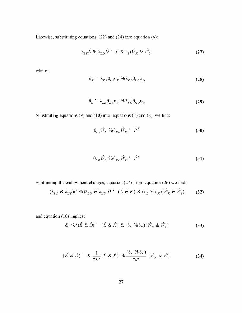
Likewise, substituting equations (22) and (24) into equation (6):

where:

Substituting equations (9) and (10) into equations (7) and (8), we find:

Subtracting the endowment changes, equation (27) from equation (26) we find:

and equation (16) implies:

(θLE & θLD ) WL % (θKE & θKD ) WK ' ( P E& P D )

(WK & WL ) ' 1*θ *

( P E& P D )

( E & D ) ' &1*λ*

( L & K ) % Ω (P E& P D )

Ω '(δK % δL )*λ**θ*

(WK & WL ) ' 1*θ*

( P E& P D )

( E & D) ' &1*λ*

( L & K ) % Ω ( P E& P D )

28

(35)

(36)

(37)

(38)

(39)

(40)

Subtracting the zero profit conditions, equation (31) from equation (30) we find:

and equation (17) implies:

Substituting equation (36) into equation (34), we find an expression for the productionpossibilities frontier:

where,

Building on Jones' description of production, there are four key equation in the 1-2-2-3model, expressed in log differentiated form:

Contract curve:

Supply:

(M & D ) ' &σQ (P M& P D )

( E & M ) ' P M& P E

& Φ

D ' E %1*λ*

( L & K ) & Ω ( P E& P D )

D ' M % σQ (P M& P D )

( E & M ) ' &1*λ*

( L & K ) % Ω (P E& P D ) % σQ (P M

& P D )

( P E& P D ) ' [ ( E & M ) % 1

*λ*( L & K ) & σQ ( P M

& P D ) ] 1Ω

( P E& P D ) ' 1

Ω[ ( P M

& P E& Φ ) % 1

*λ*( L & K ) & σQ (P M

& P D ) ]

29

(41)

(42)

(43)

(44)

(45)

(46)

(47)

Demand:

Balance of Trade:

Rearranging equation (40), the supply equation, we find:

Likewise, rearranging equation (41), the demand equation, we find:

Combining equations (43) and (44):

or,

Combining this with the balance of trade equation (42):

P E& P D ) ' 1

Ω[ (1 & σq )( P M

& P E ) & Φ %1*λ*

( L & K ) & σQ ( P E& P D )

( P E& P D ) ' 1

(σQ % Ω )[ (σQ & 1)( P E

& P M ) & Φ %1*λ*

( L & K ) ]

(WK & WL ) ' 1*θ*

1(σQ % Ω )

[ (σQ & 1)( P E& P M ) & Φ %

1*λ*

( L & K ) ]

30

(48)

(49)

(50)

Substituting equation (49) for the price term in the contract curve, equation (39), we find:

31

List of Discussion Papers

No. 40 - "Parameter Estimation for a Computable General Equilibrium Model: AMaximum Entropy Approach" by Channing Arndt, Sherman Robinson andFinn Tarp (February 1999)

No. 41 - "Trade Liberalization and Complementary Domestic Policies: A Rural-UrbanGeneral Equilibrium Analysis of Morocco" by Hans Löfgren, Moataz El-Saidand Sherman Robinson (April 1999)

No. 42 - "Alternative Industrial Development Paths for Indonesia: SAM and CGEAnalysis" by Romeo M. Bautista, Sherman Robinson and Moataz El-Said(May 1999)

No. 43* - "Marketing Margins and Agricultural Technology in Mozambique" byChanning Arndt, Henning Tarp Jensen, Sherman Robinson and Finn Tarp(July 1999)

No. 44 - "The Distributional Impact of Macroeconomic Shocks in Mexico: ThresholdEffects in a Multi-Region CGE Model" by Rebecca Lee Harris (July 1999)

No. 45 - "Economic Growth and Poverty Reduction in Indochina: Lessons From EastAsia" by Romeo M. Bautista (September 1999)

No. 46* - "After the Negotiations: Assessing the Impact of Free Trade Agreements inSouthern Africa" by Jeffrey D. Lewis, Sherman Robinson and KarenThierfelder (September 1999)

No. 47* - "Impediments to Agricultural Growth in Zambia" by Rainer Wichern, UlrichHausner and Dennis K. Chiwele (September 1999)

No. 48 - "A General Equilibrium Analysis of Alternative Scenarios for Food SubsidyReform in Egypt" by Hans Lofgren and Moataz El-Said (September 1999)

No. 49*- “ A 1995 Social Accounting Matrix for Zambia” by Ulrich Hausner(September 1999)

32

No. 50 - “Reconciling Household Surveys and National Accounts Data Using a CrossEntropy Estimation Method” by Anne-Sophie Robilliard and ShermanRobinson (November 1999)

No. 51 - “Agriculture-Based Development: A SAM Perspective on Central Viet Nam”by Romeo M. Bautista (January 2000)

No. 52 - “Structural Adjustment, Agriculture, and Deforestation in the SumateraRegional Economy” by Nu Nu San, Hans Löfgren and Sherman Robinson(March 2000)

No. 53 - “Empirical Models, Rules, and Optimization: Turning Positive Economics onits Head” by Andrea Cattaneo and Sherman Robinson (April 2000)

No. 54 - “Small Countries and the Case for Regionalism vs. Multilateralism” by Mary E. Burfisher, Sherman Robinson and Karen Thierfelder (May 2000)

No. 55 - “Genetic Engineering and Trade: Panacea or Dilemma for Developing Countries” by Chantal Pohl Nielsen, Sherman Robinson and Karen

Thierfelder (May 2000)

No. 56 - “An International, Multi-region General Equilibrium Model of AgriculturalTrade Liberalization in the South Mediterranean NIC’s, Turkey, and theEuropean Union” by Ali Bayar, Xinshen Diao and A. Erinc Yeldan (May2000)

No. 57* - “Macroeconomic and Agricultural Reforms in Zimbabwe: Policy Complementarities Toward Equitable Growth” by Romeo M. Bautista andMarcelle Thomas (June 2000)

No. 58 - “Updating and Estimating a Social Accounting Matrix Using Cross EntropyMethods ” by Sherman Robinson, Andrea Cattaneo and Moataz El-Said(August 2000)

No. 59 - “Food Security and Trade Negotiations in the World Trade Organization : ACluster Analysis of Country Groups ” by Eugenio Diaz-Bonilla, MarcelleThomas, Andrea Cattaneo and Sherman Robinson (November 2000)

33

No. 60* - “Why the Poor Care About Partial Versus General Equilibrium Effects Part 1:Methodology and Country Case’’ by Peter Wobst (November 2000)

No. 61 - “Growth, Distribution and Poverty in Madagascar : Learning from a Microsimulation Model in a General Equilibrium Framework ” by DenisCogneau and Anne-Sophie Robilliard (November 2000)

No. 62 - “Farmland Holdings, Crop Planting Structure and Input Usage: An Analysis ofChina’s Agricultural Census” by Xinshen Diao, Yi Zhang and AgapiSomwaru (November 2000)

No. 63 - “Rural Labor Migration, Characteristics, and Employment Patterns: A StudyBased on China’s Agricultural Census” by Francis Tuan, Agapi Somwaru andXinshen Diao (November 2000)

No. 64 - “GAMS Code for Estimating a Social Accounting Matrix (SAM) Using CrossEntropy (CE) Methods” by Sherman Robinson and Moataz El-Said (December2000)

No. 65 - “A Computable General Equilibrium Analysis of Mexico’s AgriculturalPolicy Reforms” by Rebecca Lee Harris (January 2001)

No. 66 - “Distribution and Growth in Latin America in an Era of Structural Reform”by Samuel A. Morley (January 2001)

No. 67 - “What has Happened to Growth in Latin America” by Samuel A. Morley (January 2001)

No. 68 - “China’s WTO Accession: Conflicts with Domestic Agricultural Policies andInstitutions” by Hunter Colby, Xinshen Diao and Francis Tuan (January2001)

No. 69 - “A 1998 Social Accounting Matrix for Malawi” by Osten Chulu and PeterWobst (February 2001)

No. 70 - “A CGE Model for Malawi: Technical Documentation” by Hans Löfgren(February 2001)

No. 71 - “External Shocks and Domestic Poverty Alleviation: Simulations with a CGEModel of Malawi” by Hans Löfgren with Osten Chulu, Osky Sichinga,Franklin Simtowe, Hardwick Tchale, Ralph Tseka and Peter Wobst (February2001)

34

No. 72 - “Less Poverty in Egypt? Explorations of Alternative Pasts with Lessons for theFuture” by Hans Löfgren (February 2001)

No. 73 - “Macro Policies and the Food Sector in Bangladesh: A General EquilibriumAnalysis” by Marzia Fontana, Peter Wobst and Paul Dorosh (February2001)

No. 74 - “A 1993-94 Social Accounting Matrix with Gender Features for Bangladesh”by Marzia Fontana and Peter Wobst (April 2001)

No. 75 - “ A Standard Computable General Equilibrium (CGE) Model” by HansLöfgren, Rebecca Lee Harris and Sherman Robinson (April 2001)

No. 76 - “ A Regional General Equilibrium Analysis of the Welfare Impact of CashTransfers: An Analysis of Progresa in Mexico” by David P. Coady andRebecca Lee Harris (June 2001)

No. 77 - “Genetically Modified Foods, Trade, and Developing Countries” by Chantal Pohl Nielsen, Karen Thierfelder and Sherman Robinson (August 2001)

No. 78 - “The Impact of Alternative Development Strategies on Growth and Distribution: Simulations with a Dynamic Model for Egypt” by Moataz El-Said, Hans Löfgren and Sherman Robinson (September 2001)

No. 79 - “Impact of MFA Phase-Out on the World Economy an Intertemporal, Global General Equilibrium Analysis” by Xinshen Diao and Agapi Somwaru (October 2001)

No. 80* - “Free Trade Agreements and the SADC Economies” by Jeffrey D. Lewis, Sherman Robinson and Karen Thierfelder (November 2001)

No. 81 - “WTO, Agriculture, and Developing Countries: A Survey of Issues” byEugenio Díaz-Bonilla, Sherman Robinson, Marcelle Thomas and Yukitsugu Yanoma (January 2002)

No. 82 - “WTO, food security and developing countries” by Eugenio Díaz-Bonilla, Marcelle Thoms and Sherman Robinson (November 2001)

No. 83 - “Economy-wide effects of El Niño/Southern Oscillation ENSO in Mexico andthe role of improved forecasting and technological change” by RebeccaLee Harris and Sherman Robinson (November 2001)

No. 84 - “Land Reform in Zimbabwe: Farm-level Effects and Cost-Benefit Analysis”by Anne-Sophie Robilliard, Crispen Sukume, Yuki Yanoma and HansLöfgren (December 2001: Revised May 2002)

No. 85 - “Developing Country Interest in Agricultural Reforms Under the World Trade Organization” by Xinshen Diao, Terry Roe and Agapi somwaru (January 2002)

No. 86 - “Social Accounting Matrices for Vietnam 1996 and 1997” by Chantal Pohl Nielsen (January 2002)

No. 87 - “How China’s WTO Accession Affects Rural Economy in the Less- Developed Regions: A Multi-Region, General Equilibrium Analysis” by Xinshen Diao, Shenggen Fan and Xiaobo Zhang (January 2002)

No. 88 - “HIV/AIDS and Macroeconomic Prospects for Mozambique: An Initial Assessment” by Channing Arndt (January 2002)

No. 89 - “International Spillovers, Productivity Growth and Openness in Thailand: An Intertemporal General Equilbrium Analysis” by Xinshen Diao, Jørn Rattsø and Hildegunn Ekroll Stokke (February 2002)

No. 90 - “Scenarios for Trade Integration in the Americas” by Xinshen Diao, Eugenio Díaz-Bonilla and Sherman Robinson (February 2002)

No. 91 - “Assessing Impacts of Declines in the World Price of Tobacco on China, Malawi, Turkey, and Zimbabwe” by Xinshen Diao, Sherman Robinson, Marcelle Thomas and Peter Wobst (March 2002)

No. 92* - “The Impact of Domestic and Global Trade Liberalization on Five

Southern African Countries” by Peter Wobst (March 2002)

No. 93 - “Trade and tradability: Exports, imports, and factor markets in the Salter-Swan model ” by Karen Thierfelder and Sherman Robinson (May 2002)

TMD Discussion Papers marked with an ‘*’ are MERRISA-related. Copies can be obtained bycalling Maria Cohan at 202-862-5627 or e-mail: