Trade and Domestic Policies in Models with Monopolistic

Collaborative Research Center Transregio 224 - www.crctr224.de

Rheinische Friedrich-Wilhelms-Universität Bonn - Universität Mannheim

Discussion Paper No. 049

Project B 06

Trade and Domestic Policies in Models with Monopolistic

Competition

Alessia Campolmi*

Harald Fadinger**

Chiara Forlati***

October 2018

*Universit_a di Verona, Department of Economics, via Cantarane 24, 37129 Verona, Italy. [email protected]

**University of Mannheim, Department of Economics, L7 3-5, D-68131 Mannheim, Germany and Centre for Economic

Policy Research (CEPR), [email protected]

***University of Southampton, School of Social Science, S017 1BJ Southampton, UK. [email protected]

Funding by the Deutsche Forschungsgemeinschaft (DFG, German Research Foundation)

through CRC TR 224 is gratefully acknowledged.

Discussion Paper Series – CRC TR 224

Trade and Domestic Policies

in Models with Monopolistic Competition∗

Alessia Campolmi† ‡

Universita di Verona

Harald Fadinger§

University of Mannheim and CEPR

Chiara Forlati¶

University of Southampton

September 2018

Abstract

We consider unilateral and strategic trade and domestic policies in single and multi-sector versions ofmodels with CES preferences and monopolistic competition featuring homogeneous (Krugman, 1980) orheterogeneous firms (Melitz, 2003). We first solve the world-planner problem to identify the efficiencywedges between the planner and the market allocation. We then derive a common welfare decompositionin terms of macro variables that incorporates all general-equilibrium effects of trade and domestic policiesand decomposes them into consumption and production-efficiency wedges and terms-of-trade effects. Weshow that the Nash equilibrium when both domestic and trade policies are available is characterized byfirst-best-level labor subsidies that achieve production efficiency, and inefficient import subsidies and exporttaxes that aim at improving domestic terms of trade. Since the terms-of-trade externality is the onlybeggar-thy-neighbor motive, it remains the only reason for signing trade agreements in this general class ofmodels. Finally, we show that when trade agreements only limit the strategic use of trade taxes but do notrequire coordination of domestic policies, the latter are set inefficiently in the Nash equilibrium in order tomanipulate the terms of trade.

Keywords: Heterogeneous Firms, Trade Policy, Domestic Policy, Trade Agreements, Terms ofTrade, Efficiency, Tariffs and Subsidies

JEL classification codes: F12, F13, F42

∗We thank Jan Haaland and seminar participants in Glasgow, Mannheim, Norwegian School of Economics, Southampton andconference participants at EEA, ETSG, the CRC TR 224 conference, the Midwest International Trade Conference and ESEM foruseful comments.

†Universita di Verona, Department of Economics, via Cantarane 24, 37129 Verona, Italy. [email protected].‡Alessia Campolmi is a Visiting Fellow at the European University Institute and is thankful for their hospitality.§University of Mannheim, Department of Economics, L7 3-5, D-68131 Mannheim, Germany and Centre for Economic Policy

Research (CEPR), [email protected]. Harald Fadinger gratefully acknowledges the hospitality of CREI. Fundingby the German Research Foundation (DFG) through CRC TR 224 is gratefully acknowledged.

¶University of Southampton, School of Social Science, S017 1BJ Southampton, UK. [email protected].

1

1 Introduction

A fundamental challenge in the research on trade policy is to understand the purpose of trade agreements. In

particular, as a prerequisite for the optimal design of trade agreements, one needs to characterize the interna-

tional externalities that can be solved by coordinating countries’ decisions (Bagwell and Staiger, 2016). In the

context of perfectly competitive neoclassical trade models, a large literature has shown that trade agreements

solve a terms-of-trade externality. Uncoordinated individual-country policy makers try use trade taxes, such

as tariffs, to manipulate international prices in their favor. This leads to a Prisoners’ Dilemma and countries

end up with inefficiently high trade taxes in equilibrium (Bagwell and Staiger, 1999, 2016). Surprisingly, it is

still not well understood if these results on the purpose of trade agreements also apply to the workhorse model

of modern international trade theory – the monopolistic competition model with heterogeneous firms (Melitz,

2003).

Moreover, with the fall of tariff barriers during the last decades, the focus of recent trade negotiations –

both at the multilateral1 and at the regional level2 – has shifted away from trade tax reductions towards

coordination of domestic policies (e.g. sector-specific policies, product market regulation, labor standards,...).

The Melitz (2003) model provides a natural framework for studying the role of these policies in the context of

trade agreements, since distortions induced by imperfect competition may lead to inefficiencies in the market

allocation, thus calling for domestic regulation (e.g., sector-specific subsidies). We investigate if domestic policies

induce additional motives for signing trade agreements beyond the classical terms-of-trade externality (Bagwell

and Staiger, 2016). Importantly, we also investigate the distortions that arise from limiting trade agreements to

the coordination of trade taxes and study if clauses requiring coordination of domestic policies or proscribing

their use should be incorporated into trade agreements.

Our first main result is that neither the presence of firm heterogeneity nor domestic policies affect the standard

wisdom from perfectly competitive models that the only motive for signing trade agreements are terms-of-trade

externalities. When countries can set both domestic and trade policies strategically, domestic policies are set

efficiently, while trade taxes are used to manipulate the terms of trade. Our second main result is that when

trade agreements only limit countries’ ability to use trade taxes strategically but do not require coordination

of domestic policies, individual-country policy makers set domestic policies inefficiently because they face a

trade-off between correcting domestic inefficiencies and manipulating their terms of trade. In order to achieve

these conclusions, we proceed as follows.

Our theoretical setup features two countries, CES preferences and either a single or multiple sectors. Firms

operate under monopolistic competition and are potentially heterogeneous in terms of productivity. In the ver-

sion with heterogeneous firms we allow firm-specific productivity levels to be drawn from arbitrary productivity

1The Doha round of multilateral WTO negotiations deals with issues such as environmental regulation and intellectual propertyrights and initially also included competition policy and government procurement.

2E.g., the European Union’s strategy is to sign ”deep” bilateral trade agreements that cover a host of areas in addition toclassical tariff reduction, such as domestic regulation, foreign direct investment and intellectual property rights. Recent examplesare the trade agreements with Canada, Korea and Japan.

2

distributions. Policy makers in each country can set both sector-specific trade policies (import and export taxes)

and domestic policies (labor taxes). We use the insight of Arkolakis, Costinot and Rodrıguez-Clare (2012) that

monopolistic competition models with CES preferences have a common macro representation in terms of sec-

toral aggregate bundles. This representation also makes clear that in this class of models the welfare-relevant

terms of trade are defined in terms of aggregate price indices of importables and exportables. As a consequence,

policy instruments can affect the terms of trade both by changing the international prices of individual varieties

(directly and indirectly via selection) and by impacting on the measure of firms active in foreign markets.

We first solve for the allocation chosen by a social planner whose objective is to maximize world welfare in order

to identify the welfare wedges present in the market allocation. Following the approach of Costinot, Rodrıguez-

Clare and Werning (2016), we separate the planner problem into different stages: a micro stage; a macro stage

within sectors; and a cross-sector macro stage. At the micro stage, the planner chooses how much to produce of

each differentiated variety given the sectoral aggregates. We show that given CES preferences, the solution to

the micro problem always corresponds to the market allocation, i.e., relative firm size is always optimal. In the

within-sector macro stage, the planner chooses for each sector how much to produce of the aggregate bundle that

is domestically produced and consumed and how much to produce of the aggregate exportable bundle. Here,

a consumption-efficiency wedge arises between the planner and the market allocation whenever trade policy

instruments are used.3 Finally, the cross-sector macro stage is present only in the multi-sector version of the

model. At this stage, the planner determines the optimal allocation across macro sectors. The cross-sectoral

allocation corresponds to the market allocation if and only if trade taxes are not used and monopolistic markups

are offset with labor subsidies, otherwise too little labor is allocated to the monopolistically competitive sector

and a production-efficiency wedge is present.

We then turn to the problem of a benevolent policy maker who is concerned with maximizing world welfare and

can set labor and trade taxes. By using the total-differential approach to optimization, we are able to derive an

exact welfare decomposition in terms of macro aggregates that decomposes general-equilibrium welfare effects

of trade and domestic policies and simultaneously identifies the optimality conditions of the world policy maker.

Welfare effects can be decomposed into three terms: (i) a consumption-efficiency wedge, (ii) a production-

efficiency wedge and (iii) terms-of-trade effects. This decomposition is useful for the following reasons: The

efficiency terms in the welfare decomposition correspond exactly to the wedges between the planner and the

market allocation mentioned above. As a result, solving the problem of the world policy maker is equivalent

to setting both consumption and production-efficiency wedges in the welfare decomposition equal to zero.

Moreover, in the symmetric equilibrium terms-of-trade motives of individual countries offset each other at the

world level: an improvement in the terms of trade of one country necessarily implies an equivalent terms-of-trade

worsening of the other. Thus, terms-of-trade effects are a pure beggar-thy-neighbor incentive and hence the

world policy maker disregards them. We show that in the one-sector version of the model production efficiency is

always guaranteed and the world-policy-maker solution corresponds to the (Pareto-optimal) free-trade allocation.

3Dhingra and Morrow (2019) establish efficiency of the market allocation in a closed-economy one-sector version of Melitz underCES preferences.

3

By contrast, in the presence of multiple sectors the world policy maker closes the production-efficiency wedge

and implements the planner allocation using sector-specific labor subsidies.

Next, we study trade and domestic policies from the individual-country perspective. Our welfare decomposition

makes apparent that in the one-sector version of the model unilateral policies are driven unequivocally by

a trade-off between improving domestic terms of trade and creating consumption wedges, while production

efficiency is automatically guaranteed. By contrast, in the multi-sector version of the model, closing the domestic

production-efficiency wedge becomes an additional motive for individual-country policy makers.

As a preparation for the case of strategic interaction, we study how unilateral policy deviations in individual

instruments affect the terms of trade and production efficiency. We show that in the one-sector model, where

labor supply is completely inelastic, a small unilateral import tariff is welfare enhancing from the unilateral

perspective compared to free trade. A tariff improves domestic terms of trade by increasing the relative wage.

In the presence of firm heterogeneity there are two additional opposing effects: an improvement in the terms of

trade stemming from an increase in the variable-profit share arising from exports and a terms-of-trade worsening

from tougher selection into exporting. Differently, in the multi-sector model with a linear outside good labor

supply is perfectly elastic and a tariff worsens domestic terms of trade by increasing labor demand for the

differentiated bundles and triggering entry into that sector. This reduces the relative price of exportables via

the extensive margin. In the presence of firm heterogeneity there are again two additional opposing effects:

changes in the variable-profit share arising from exports and changes in selection into exporting. At the same

time, when starting from the free-trade allocation, a tariff improves production efficiency by increasing the

amount of labor allocated to the differentiated sector. Similarly, a labor or export subsidy also improves

production efficiency, while worsening the terms-of-trade. Thus, using any individual policy instrument gives

rise to a trade-off between reducing the production-efficiency wedge and worsening the terms of trade.

We also investigate the role of firm heterogeneity in shaping unilateral policies in the multi-sector model. With

homogeneous firms a small tariff is always welfare improving from the unilateral perspective because the increase

in production efficiency always dominates the negative terms-of-trade effect. By contrast, in the presence of

heterogeneous firms and selection into exporting the sign of the welfare effects stemming from unilateral policy

changes – and thus whether a tariff or an import subsidy is unilaterally beneficial – depends on the average

variable profit share from sales in the domestic market. Intuitively, if the bulk of variable profits are made

domestically, increases in domestic production efficiency dominate negative terms-of-trade effects, while the

opposite is the case if the larger part of profits arises from exporting. Thus, these results for unilateral policy

changes suggest that firm heterogeneity can affect trade policy qualitatively.

We then return to the question if domestic policies provide an additional reason for signing free-trade agreements

beyond terms-of-trade externalities. This would be the case if uncoordinated policy makers set them inefficiently,

thereby imposing externalities on the other country. We thus characterize the Nash equilibrium of the policy

game in the multi-sector model where individual-country policy makers set both trade and domestic policies

simultaneously. We show that the equilibrium policies consist of the first-best level of labor subsidies that close

4

production-efficiency wedges and inefficient import subsidies and export taxes that aim at improving the terms

of trade. This implies that domestic policies do not create any additional motive for trade agreements since

production inefficiencies are completely internalized by individual-country policy makers.4. Here, we show that

it carries over to trade models with monopolistic competition and heterogeneous firms. Moreover –in contrast

to unilateral policies – the sign of the Nash-equilibrium trade policies (import subsidies and export taxes) does

not depend on firm heterogeneity.

Finally, we turn to the design of trade agreements in the presence of domestic policies. A globally efficient

outcome requires cooperation on trade and domestic policies. We show that when trade agreements only limit

the strategic use of trade-policy instruments but do not require coordination of domestic policies, individual-

country policy makers use domestic policies both to increase production efficiency and to manipulate the terms

of trade. Specifically, we study the Nash equilibrium of a policy game, where only domestic policies can be

set strategically, while trade policy instruments are not available. In this situation, firm heterogeneity has a

qualitative impact on the Nash policies: the Nash policy outcome depends on the variable-profit share from

domestic sales. When at least half of the profits of the average active firm are made in the domestic market

or when firms are homogeneous, the production-efficiency effect dominates and the Nash equilibrium features

(inefficiently low) labor subsidies. In this case a trade agreement that prohibits the use of both trade and

domestic policies provides lower welfare than an agreement that eliminates trade taxes but allows countries

to choose domestic policies strategically. By contrast, when more than half of the average firm’s profits arise

from exports, the terms-of-trade effect dominates and the Nash equilibrium features labor taxes. Intuitively,

the smaller the profit share from domestic sales, the more open the economy is and thus the larger the incentive

to exploit international externalities. In this case a trade agreement that prohibits the use of both trade and

domestic policies fares better in welfare terms than one that eliminates trade taxes but allows countries to set

domestic policies strategically. Finally, we show that when variable or fixed physical trade costs fall and therefore

the profit share from exporting rises, welfare gains from integrating cooperation on domestic policies into trade

agreements become proportionally larger.Thus, the case for deep trade agreements that require coordination of

domestic regulation becomes stronger when physical trade barriers are lower.

The rest of the paper is structured as follows. In the next subsection we briefly discuss the related literature.

In Section 2 we describe a standard multi-sector Melitz (2003) model expressed in terms of macro bundles. In

Section 3 we then set up and solve the problem of a planner who is concerned with maximizing world welfare.

We separate it into a micro, a within-sector macro and a cross-sector macro stage and compare each stage to

the market allocation in order to identify the relevant efficiency wedges. Next, in Section 4 we solve the problem

of a world policy maker who is concerned with maximizing world welfare and disposes of trade and labor taxes.

As an intermediate step of solving this problem, we derive a welfare decomposition that decomposes welfare

effects of policy instruments into a consumption wedge, a production wedge and terms of trade effects. We then

show that solving the world-policy-maker problem is equivalent to setting all wedges individually equal to zero.

4This result is an application of the targeting principle, which is known to hold in perfectly competitive trade models (Ederington,2001)

5

In Section 5 we turn to the problem of individual-country policy makers, derive individual-country welfare and

discuss welfare effects of unilateral policy deviations. Finally, we consider strategic trade and domestic policies.

We first characterize the Nash equilibrium of the policy game where individual-country policy makers set both

trade and labor taxes simultaneously and strategically. We then turn to the Nash equilibrium of the policy

game when only labor taxes can be set strategically. Section 6 presents our conclusions.

1.1 Related literature

Several theoretical contributions have studied the incentives for trade policy in single and multiple-sector versions

of the Krugman (1980) and Melitz (2003) models and have identified numerous mechanisms through which trade

policy affects outcomes in these models.

Specifically, Gros (1987) and Helpman and Krugman (1989) examine the one-sector version of the Krugman

(1980) model with homogeneous firms. They identify a terms-of-trade motive for strategic tariffs, which increase

domestic factor prices. By contrast, studies investigating trade policy in the two-sector version of Krugman

(1980) – which features a linear outside sector that pins down factor prices – typically find that strategic

tariffs are due to a home market/production-relocation motive (Venables, 1987; Helpman and Krugman, 1989;

Ossa, 2011). More recently, Campolmi, Fadinger and Forlati (2012), allow for the simultaneous choice of labor,

import and export taxes in this model. They show that the tariff result found by previous studies is due to

a missing instrument problem. Once policy makers dispose of enough instruments the strategic equilibrium is

characterized by the first-best level of labor subsidies, import subsidies and export taxes that aim at improving

domestic terms of trade (Campolmi, Fadinger and Forlati, 2014).

A small number of studies analyze trade policy in the Melitz (2003) model with a single sector. Demidova

and Rodrıguez-Clare (2009) and Haaland and Venables (2016) investigate optimal unilateral trade policy in

a small-open-economy version of Melitz (2003) with Pareto-distributed productivity. While Demidova and

Rodrıguez-Clare (2009) identify a distortion in the relative price of imported varieties (markup distortion) and

a distortion on the number of imported varieties (entry distortion) as motives for unilateral policy, Haaland

and Venables (2016) single out terms-of-trade effects as the only motive for individual-country trade policy.

Similarly, Felbermayr, Jung and Larch (2013), who consider strategic import taxes in a two-country version

of this model, identify the same motives for tariffs as Demidova and Rodrıguez-Clare (2009). Haaland and

Venables (2016) also study unilateral policy in the two-sector small-open-economy variant of Melitz (2003)

with Pareto-distributed productivities and identify terms-of-trade externalities and monopolistic distortions as

drivers of unilateral policy.

Our contribution is to show that the welfare incentives for trade policy in the previous models can be understood

using a common welfare decomposition in terms of macro aggregates. This approach makes clear that the terms-

of-trade motive is the only externality that needs be addressed by trade agreements in this class of models.

Also closely related is Costinot et al. (2016), who consider unilateral trade policy in a generalized two-country

6

version of Melitz (2003). Similarly to our approach, they consider the macro representation of the model and

define the terms of trade in terms of aggregate bundles of importables and exportables. They investigate

unilaterally optimal firm-specific and non-discriminatory policies and establish terms-of-trade effects as the

motive for trade policy. Their main interest is to investigate how firm heterogeneity shapes trade policy. They

show that, conditional on the elasticity of substitution and the share of expenditure on local goods abroad,

firm heterogeneity reduces the optimal tariff if and only if it leads to non-convexities in the foreign production

possibility frontier.

We consider our analysis as complementary to theirs. In particular, we show that the incentives for using trade

and domestic policies in models with CES preferences and monopolistic competition can be analyzed with a

common welfare decomposition. Their approach of using optimal tax formulas is convenient for evaluating the

quantitative impact of firm heterogeneity but makes it difficult to isolate policy makers’ welfare incentives, in

particular when the set of policy instruments is insufficient to address all distortions separately. Most impor-

tantly, while their analysis is limited to unilaterally optimal policies we consider the case of strategic interaction

and compare Nash equilibrium domestic and trade policies to the outcome of a world policy maker. Finally,

while Costinot et al. (2016) find that firm heterogeneity potentially affects unilateral trade taxes both quanti-

tatively and qualitatively compared to homogeneous-firm models, we uncover that the sign of the equilibrium

strategic taxes is unaffected by the presence of firm heterogeneity as long as the set of instruments is sufficiently

large.

This paper is also closely connected to the vast literature on trade policy in perfectly competitive trade models

(Dixit, 1985). We show that many insights from this literature carry over to models with monopolistic competi-

tion and firm heterogeneity. Specifically, the result that trade agreements solve a terms-of-trade externality also

applies in our context (Bagwell and Staiger, 2016). Moreover, also the Bhagwati-Johnson principle of targeting,

which states that optimal policy should use the instrument that operates most effectively on the appropriate

margin, remains valid.

Finally, there is also a close connection with the literature on trade and domestic policies in perfectly competitive

models. Copeland (1990) discusses the idea that in the presence of trade agreements that limit the strategic use

of tariffs individual-country policy makers have incentives to use domestic policies to manipulate their terms of

trade. Ederington (2001) considers the optimal design of self-enforceable joint agreements on trade and domestic

policies and establishes that such agreements should require full coordination of domestic policies but should

allow countries to set positive levels of tariffs, in order to mitigate incentives to deviate from cooperation.

2 The Model

The setup follows Melitz and Redding (2015). The world economy consists of two countries i: Home (H) and

Foreign (F). The only factor of production is labor which is supplied inelastically in amount L in each country,

7

perfectly mobile across firms and sectors and immobile across countries. Each country has either one or two

sectors. The first sector produces a continuum of differentiated goods under monopolistic competition with free

entry. If present, the other sector is perfectly competitive and produces a homogeneous good. Labor markets are

perfectly competitive. All goods are tradable but only the differentiated goods are subject to iceberg transport

costs. Both countries are identical in terms of preferences, production technology, market structure and size. All

variables are indexed such that the first sub-index corresponds to the location of consumption and the second

sub-index to the location of production.

2.1 Technology and Market Structure

2.1.1 Differentiated sector

Firms in the differentiated sector operate under monopolistic competition with free entry. They pay a fixed cost

in terms of labor, fE , to enter the market and to pick a draw of productivity ϕ from a cumulative distribution

G(ϕ).5 After observing their productivity draw, they decide whether to pay a fixed cost f in terms of domestic

labor to become active and produce for the domestic market. Active firms then decide whether to pay an

additional market access cost fX (in terms of domestic labor) to export to the other country, or to produce only

for the domestic market. Therefore, labor demand of firm ϕ located in market i for a variety sold in market j

is given by:

lji(ϕ) =qji(ϕ)

ϕ+ fji, i, j = H,F (1)

where

fji =

f j = i

fX j 6= i

Here qji(ϕ) is the production of a firm with productivity ϕ located in country i for market j. Varieties sold in

the foreign market are subject to an iceberg transport cost τ > 1. We thus define:

τji =

1 j = i

τ j 6= i

5 We assume that ϕ has support [0,∞) and that G(ϕ) is continuously differentiable with derivative g(ϕ).

8

2.1.2 Homogenous sector

In case the homogeneous-good sector is present, labor demand LZi for the homogenous good Z, which is

produced in both countries i with identical production technology, is given by:

LZi = QZi, (2)

where QZi is the production of the homogeneous good. Since this good is sold in a perfectly competitive

market without trade costs, its price is identical in both countries and equals the marginal cost of production

Wi. We assume that the homogeneous good is always produced in both countries in equilibrium. This implies

equalization of wages Wi = Wj for i 6= j (factor price equalization).

We also consider a version of the model without the homogeneous sector. In this case, wages across the two

countries will not necessarily be equalized.

2.2 Preferences

Households’ utility function is given by:

Ui ≡ α logCi + (1− α) logZi, i = H,F , (3)

where Ci aggregates over the varieties of differentiated goods and α is the expenditure share of the differentiated

bundle in the aggregate consumption basket. When α is set to unity, we go back to a one-sector model (Melitz,

2003). Zi represents consumption of the homogeneous good (Krugman, 1980). The differentiated varieties

produced in the two countries are aggregated with a CES function given by:6

Ci =

∑

j∈H,F

Cε−1ε

ij

εε−1

, i = H,F (4)

Cij =

[Nj

∫ ∞

ϕij

cij(ϕ)ε−1ε dG(ϕ)

] εε−1

, i, j = H,F (5)

Here, Cij is the aggregate consumption bundle of country-i consumers of varieties produced in country j, cij(ϕ)

is consumption by country i consumers of a variety ϕ produced in country j, Nj is the measure of varieties

produced by country j. ϕij is the cutoff-productivity level, such that a country-j firm with this productivity

level makes exactly zero profits when selling to country i, while firms with strictly larger productivity levels

make positive profits from selling to this market, so that all country-j firms with ϕ ≥ ϕij export to country

6Notice that we can index consumption of differentiated varieties by firms’ productivity level ϕ since all firms with a given level

of ϕ behave identically. Note also that our definitions of Cij imply Ci =[

Ni

∫∞

ϕiicii(ϕ)

ε−1ε dG(ϕ) +Nj

∫∞

ϕijcij(ϕ)

ε−1ε dG(ϕ)

]ε

ε−1

i.e., the model is the standard one considered in the literature. However, it is convenient to define optimal consumption indices.

9

i. Finally, ε > 1 is the elasticity of substitution between domestic and foreign bundles and between different

varieties.

2.3 Government

The government of each country disposes of three fiscal instruments. A labor tax/subsidy (τLi) on firms’ fixed

and marginal costs,7 a tariff/subsidy on imports (τIi) and a tax/subsidy on exports (τXi). Note that τmi

indicates a gross tax for m ∈ L, I,X, i.e., τmi < 1 indicates a subsidy and τmi > 1 indicates a tax. In what

follows, we employ the word tax whenever we refer to a policy instrument without specifying whether τmi is

smaller or larger than one and we use the following notation:

τTij =

1 i = j

τIiτXj i 6= j

(6)

Moreover, we assume that taxes are paid directly by the firms8 and that all government revenues are redistributed

to consumers through a lump-sum transfer.

2.4 Equilibrium

Since the model is standard, we relegate a more detailed description of the setup and the derivation of the market

equilibrium to Appendix A. In a market equilibrium, households choose consumption of the differentiated

bundles and – when available –the homogeneous good in order to maximize utility subject to their budget

constraint; firms in the differentiated sector choose quantities in order to maximize profits given their residual

demand schedules and enter the differentiated sector until their expected profits – before productivity realizations

are drawn – are zero; they produce for the domestic and export markets if their productivity draw is weakly

above the market-specific survival-cutoff level at which they make exactly zero profits; if present, firms in the

homogeneous-good sector price at marginal cost; governments run balanced budgets and all markets clear. We

write the equilibrium in terms of sectoral aggregates. This approach follows Campolmi et al. (2012) and Costinot

et al. (2016). Specifically, the one-sector model can be represented in terms of three aggregate goods: a good

that is domestically produced and consumed; a domestic exportable good and a domestic importable good.

The two-sector model additionally features a homogeneous good. This representation in terms of aggregate

bundles (i) highlights that models with monopolistic competition and CES preferences have a common macro

presentation and (ii) makes the connection to standard neoclassical trade models visible. It will also be useful

for interpreting the wedges between the planner and the market allocations and for our welfare decomposition.

7We impose that the same labor taxes are levied on both fixed and marginal costs (including also the fixed entry cost fE). Thisassumption is necessary to keep firm size unaffected by taxes, which turns out to be optimal, as we will show in Section 3.2.

8 In particular, following the previous literature (Venables (1987), Ossa (2011)), we assume that tariffs and export taxes arecharged ad valorem on the factory gate price augmented by transport costs. This implies that transport services are taxed.

10

Finally, the macro representation will make clear that the welfare-relevant terms of trade that policy makers

consider in their objective should be defined in terms of ideal price indices of sectoral exportables relative to

importables.

The market equilibrium can be described by the following conditions:

ϕji =

[∫ ∞

ϕji

ϕε−1 dG(ϕ)

1−G(ϕji)

] 1ε−1

, i, j = H,F (7)

δji =fji(1−G(ϕji))

(ϕji

ϕji

)ε−1

∑k=H,F

fki(1−G(ϕki))(

ϕki

ϕki

)ε−1 , i, j = H,F (8)

(ϕii

ϕij

)=

(fiifij

) 1ε−1(τLi

τLj

) εε−1(Wi

Wj

) εε−1

τ−1ij τ

− εε−1

Tij i, j = H,F, i 6= j (9)

∑

j=H,F

fji(1−G(ϕji))

(ϕji

ϕji

)ε−1

= fE +∑

j=H,F

fji(1−G(ϕji)), i = H,F (10)

Cij =

(ε− 1

ε

)(εfij)

−1ε−1 τ−1

ij ϕij (δijLCj)ε

ε−1 , i, j = H,F (11)

Pij =

(ε

ε− 1

)(εfij)

1ε−1 τijτTijτLjWjϕ

−1ij (δijLCj)

−1ε−1 , i, j = H,F (12)

L− LCi −(1− α)

α

∑

k=H,F

(PikCik) + τ−1Ij PjiCji = τ−1

Ii PijCij , i = H, j = F (13)

∑

i=H,F

(L− LCi) =1− α

α

∑

i=H,F

∑

j=H,F

PijCij (14)

Zi =(1− α)

α

∑

j=H,F

PijCij i = H,F (15)

Condition (7) defines the average productivity of country-i firms active in market j (ϕji), given by the harmonic

mean of productivity of those firms that operate in the respective market. Condition (8) defines δji, the variable-

profit share of a country-i firm with average productivity ϕji arising from sales in market j.9 Equivalently, δji

is also the share of total labor used in the differentiated sector in country i that is allocated to production

for market j. Condition (9) follows from dividing the zero-profit conditions defining the survival-productivity

cutoffs – which imply zero profits for a country-i firm with the cutoff-productivity level ϕij from selling in

market j – for firms in their domestic market by the one for foreign firms that export to the domestic market.

Condition (10) is the free-entry condition combined with the zero-profit conditions. In equilibrium, expected

variable profits (left-hand side) have to equal the expected overall fixed cost bill (right-hand side).

Condition (11) can be interpreted as a sectoral aggregate production function Cij = QCij(LCj) in terms of

aggregate labor allocated to the differentiated sector, LCj , measuring the amount of production of the aggregate

bundle produced in country j for consumption in market i. Condition (12) defines the equilibrium consumer

9It can be shown that fji(1−G(ϕji))(

ϕji

ϕji

)ε−1are variable profits of a the average country-i firm active in market j.

11

price index Pij of the aggregate differentiated bundle produced in country j and sold in country i.10

Importantly, condition (13) defines the trade-balance condition that states that the value of net imports of the

homogeneous good plus the value imports of the differentiated bundle (left-hand side) must equal the value of

exports of the differentiated bundle (right-hand side). Note that imports and exports of differentiated bundles

are evaluated at international prices (before tariffs are applied). The model-consistent definition of the terms of

trade then follows directly from this equation.11 The international price of imports τ−1Ii Pij defines the inverse

of the terms of trade of the differentiated importable bundle (relative to the homogeneous good), while the

international price of exports τ−1Ij Pji defines the terms of trade of the differentiated exportable bundle (relative

to the homogeneous good). In addition, the terms of trade of the differentiated exportable relative to the

importable bundle are given by (τ−1Ij Pji)/(τ

−1Ii Pij), which is the only relevant relative price when α = 1. Given

that terms of trade are defined in terms of sectoral ideal price indices of exportables relative to importables,

they will be affected not only by changes in the prices of individual varieties but also by changes in the measure

of exporters and importers and their average productivity levels. We will discuss this in detail in Section 5.2.

Finally, (14) is the the market-clearing condition for the homogeneous good12 and condition (15) defines demand

for the homogeneous good, presented here for future reference.

We normalize the foreign wage, Wi, i = F , to unity. Thus, we have a system of 24 equilibrium equations in

25 unknowns, namely δji, ϕji, ϕji, Cji, Pij , LCi, Zi for i, j = H,F and Wi for i = H. To close the model we

note that if α < 1, so that there exists a homogeneous sector, Wi = 1 for i = H, since factor prices must be

equalized in equilibrium; by contrast, if α = 1, so that there is only a single sector, LCi = L for i = F , since

the domestic labor market must clear.

Observe that when α < 1 the equilibrium can be solved recursively. First, we can use conditions (7), (9) and

(10) to implicitly determine the four productivity cutoffs ϕji as well as the average productivity levels in the

domestic and export market for both countries ϕji, given the values of the policy instruments. Then, we can

determine the variable profit shares of the average firm in each market δji, since they are a function of the

productivity cutoffs only. Finally, given both ϕji and δji, we can recover Cji and Pij and plug them into the

trade-balance condition and the homogeneous-good-market-clearing condition to solve for the equilibrium levels

of LCj .

Moreover, note that under some additional assumptions the equilibrium equations also nest the one-sector and

the multi-sector versions of the Krugman (1980) model with homogeneous firms and exogenous productivity

level ϕ = 1. A sufficient set of assumptions is that fji = 0 for i, j = H,F and G(ϕ) is degenerate at unity. In

this case, conditions (7), (8) (9) and (10) need to be dropped from the set of equilibrium conditions and (11)

10More precisely, if α < 1, Pij should be interpreted as a relative aggregate price index in terms of the homogeneous good.11This definition is also consistent with Campolmi et al. (2012) and Costinot et al. (2016), who also define terms of trade in terms

of aggregate international price indices of exportables and importables.12Alternatively if α = 1 it states the domestic labor-market-clearing condition.

12

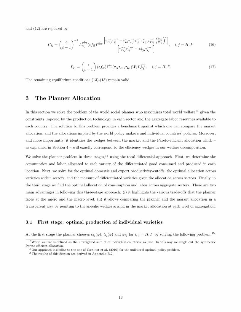
and (12) are replaced by

Cij =

(ε

ε− 1

)−1

Lε

ε−1

Cj (εfE)−1ε−1

[τ−εT ijτ

−εij − τ εLiτ

−εLj τ

−1ij τ εTjiτ

−εT ij

(Wi

Wj

)ε]

[τ−εT ijτ

1−εij − τ εTjiτ

ε−1ij

] , i, j = H,F (16)

Pij =

(ε

ε− 1

)(εfE)

1ε−1 (τijτTijτLj)WjL

−1ε−1

Cj , i, j = H,F. (17)

The remaining equilibrium conditions (13)-(15) remain valid.

3 The Planner Allocation

In this section we solve the problem of the world social planner who maximizes total world welfare13 given the

constraints imposed by the production technology in each sector and the aggregate labor resources available to

each country. The solution to this problem provides a benchmark against which one can compare the market

allocation, and the allocations implied by the world policy maker’s and individual countries’ policies. Moreover,

and more importantly, it identifies the wedges between the market and the Pareto-efficient allocation which –

as explained in Section 4 – will exactly correspond to the efficiency wedges in our welfare decomposition.

We solve the planner problem in three stages,14 using the total-differential approach. First, we determine the

consumption and labor allocated to each variety of the differentiated good consumed and produced in each

location. Next, we solve for the optimal domestic and export productivity-cutoffs, the optimal allocation across

varieties within sectors, and the measure of differentiated varieties given the allocation across sectors. Finally, in

the third stage we find the optimal allocation of consumption and labor across aggregate sectors. There are two

main advantages in following this three-stage approach: (i) it highlights the various trade-offs that the planner

faces at the micro and the macro level; (ii) it allows comparing the planner and the market allocation in a

transparent way by pointing to the specific wedges arising in the market allocation at each level of aggregation.

3.1 First stage: optimal production of individual varieties

At the first stage the planner chooses cij(ϕ), lij(ϕ) and ϕij for i, j = H,F by solving the following problem:15

13World welfare is defined as the unweighted sum of of individual countries’ welfare. In this way we single out the symmetricPareto-efficient allocation.

14Our approach is similar to the one of Costinot et al. (2016) for the unilateral optimal-policy problem.15The results of this Section are derived in Appendix B.2.

13

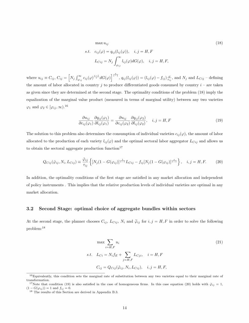
maxuij (18)

s.t. cij(ϕ) = qij(lij(ϕ)), i, j = H,F

LCij = Nj

∫ ∞

ϕij

lij(ϕ)dG(ϕ), i, j = H,F,

where uij ≡ Cij , Cij =[Nj

∫∞

ϕijcij(ϕ)

ε−1ε dG(ϕ)

] εε−1

, qij(lij(ϕ)) = (lij(ϕ)− fij)ϕτij

, and Nj and LCij – defining

the amount of labor allocated in country j to produce differentiated goods consumed by country i – are taken

as given since they are determined at the second stage. The optimality conditions of the problem (18) imply the

equalization of the marginal value product (measured in terms of marginal utility) between any two varieties

ϕ1 and ϕ2 ∈ [ϕij ,∞).16

∂uij

∂cij(ϕ1)

∂qij(ϕ1)

∂lij(ϕ1)=

∂uij

∂cij(ϕ2)

∂qij(ϕ2)

∂lij(ϕ2), i, j = H,F (19)

The solution to this problem also determines the consumption of individual varieties cij(ϕ), the amount of labor

allocated to the production of each variety lij(ϕ) and the optimal sectoral labor aggregator LCij and allows us

to obtain the sectoral aggregate production function17

QCij(ϕij , Ni, LCij) ≡ϕij

τij

[Nj(1−G(ϕij)]

1ε−1LCij − fij [Nj(1−G(ϕij)]

εε−1

, i, j = H,F. (20)

In addition, the optimality conditions of the first stage are satisfied in any market allocation and independent

of policy instruments . This implies that the relative production levels of individual varieties are optimal in any

market allocation.

3.2 Second Stage: optimal choice of aggregate bundles within sectors

At the second stage, the planner chooses Cij , LCij , Ni and ϕij for i, j = H,F in order to solve the following

problem:18

max∑

i=H,F

ui (21)

s.t. LCi = NifE +∑

j=H,F

LCji, i = H,F

Cij = QCij(ϕij , Ni, LCij), i, j = H,F,

16Equivalently, this condition sets the marginal rate of substitution between any two varieties equal to their marginal rate oftransformation.

17Note that condition (19) is also satisfied in the case of homogeneous firms. In this case equation (20) holds with ϕij = 1,(1−G(ϕij)) = 1 and fij = 0.

18 The results of this Section are derived in Appendix B.3.

14

where ui = logCi, Ci is given by (4) and Qij(ϕij , Ni, LCij) is defined in (20). The first-order conditions of the

above problem lead to the following conditions:

∂ui

∂Cii

∂QCii

∂LCii=

∂uj

∂Cji

∂QCji

∂LCji, i, j = H,F, i 6= j (22)

fE =∑

j=H,F

∂QCji/∂Ni

∂QCji/∂LCji, i = H,F (23)

∂QCji

∂ϕji= 0, i, j = H,F (24)

Condition (22) states that the marginal value product of labor of the bundle produced and consumed domesti-

cally (measured in terms of domestic marginal utility) has to equal the marginal value product of labor of the

domestic exportable bundle (measured in terms of foreign marginal utility).19

Condition (23) captures the trade-off between the extensive and intensive margins of production. Creating an

additional variety (firm) requires fE units of labor in terms of entry cost. This additional variety marginally

increases output of the domestically produced and consumed and the exportable bundles at the extensive margin

but comes at the opportunity cost of reducing the amount of production of existing varieties (intensive margin),

since aggregate labor has to be withdrawn from these production activities.

Condition (24) reveals the trade-off between increasing average productivity and reducing the number of active

firms. From the aggregate production function (20), an increase in ϕji on the one hand increases sectoral

production by making the average firm more productive, on the other hand it decreases sectoral production by

reducing the measure of firms that are above the cutoff-productivity level ϕji. At the margin, these two effects

have to offset each other exactly.

By combining (20), (23) and (24), we obtain a sectoral production function for QCji in terms of aggregate labor

LCi:

QCji(LCi) =

(ε− 1

ε

)(εfji)

−1ε−1 τ−1

ji ϕji (δjiLCi)ε

ε−1 , i, j = H,F (25)

This equation corresponds exactly to condition (11) for the market allocation. Thus, consumption of the

aggregate differentiated bundles is efficient in any market allocation conditional on the cutoffs ϕji and the

amount of aggregate labor allocated to the differentiated sector LCi.20

We now compare the planner’s optimality conditions for the second stage with those of the market allocation.

Even in a symmetric market allocation condition (22) is not satisfied, i.e., there is a wedge between the marginal

19Equivalently, this condition states that the marginal rate of substitution (in terms of home versus foreign utility) between thedomestically produced and consumed bundle and the domestic exportable bundle has to equal the marginal rate of transformationof these bundles.

20Note that the planner’s optimality conditions are also valid for the case of homogeneous firms with ϕij = 1 exogenous, sothat the first-order conditions are given by (22) and (23) only. Equation (25) also holds with fij = fE , ϕij = 1 and δji =[

1 + τε−1ij

(

Cj

Ci

)ε−1]

1−εε

.

15

value product of labor of the domestically produced and consumed bundle and the marginal value product of

labor of the exportable bundle (both evaluated in terms of marginal utility of the consuming country) whenever

τTji 6= 1:

∂ui

∂Cii

∂QCii

∂LCii=

∂uj

∂Cji

∂QCji

∂LCji(τTji)

1−ε, i, j = H,F, i 6= j. (26)

Thus, a foreign tariff (τIj > 1) or a domestic export tax (τXi > 1) imply that the marginal value product on the

right-hand side must increase relative to the one on the left-hand side, which happens when foreign consumers

reduce imports and home consumers increase consumption of the domestically produced bundle. As a result,

production and consumption is inefficiently tilted towards the domestically produced bundle.21 By contrast,

one can show that conditions (23)22 and (24) are satisfied in any market allocation.

Alternatively, one can also compare the planner solution with the market outcome in terms of allocations. For

the heterogeneous-firm model it turns out that efficiency of the cutoff-productivity levels ϕij is sufficient for

the market allocation to coincide with the planner solution for the second stage. Simultaneously, a distortion

of the cutoffs implies that all equilibrium outcomes are distorted. Notice that according to conditions (7)-

(10) distortions of the cutoffs are exclusively due to trade taxes. From (9), in a symmetric equilibrium, the

cutoff-productivity levels in the market are determined by:

(ϕii

ϕji

)=

(fiifji

) 1ε−1

τ−1ji τ

− εε−1

Tji i = H,F, j 6= F

Thus, the cutoff-productivity levels ϕii and ϕji are efficient in the free-trade allocation, i.e. ϕFTji = ϕFB

ji , while

there is a distortion induced on ϕji whenever trade taxes are used (when τTji = τIjτXi 6= 1). In particular,

τTji > 1 implies that ϕii/ϕji is too small relative to the efficient level, so that the marginal exporter is too

productive relative to the least productive domestic producer.

3.3 Third stage: allocation across sectors

The third stage is present only in the case of multiple sectors (α < 1). In this stage, the planner chooses Cij

and Zi for i, j = H,F , and the amount of aggregate labor allocated to the differentiated sector LCi to solve the

21Observe that this wedge is present independently of firm heterogeneity.22This condition is satisfied in any market allocation as long as the same labor tax is charged on marginal and fixed costs.

16

following maximization problem:23

max∑

i=H,F

Ui (27)

s.t. Cij = QCij(LCj), i, j = H,F

QZi = QZi(L− LCi), i = H,F∑

i=H,F

QZi =∑

i=H,F

Zi,

where Ui is given by (3) and (4), QZi(L− LCi) = L− LCi and QCij(LCj) is defined in (25).

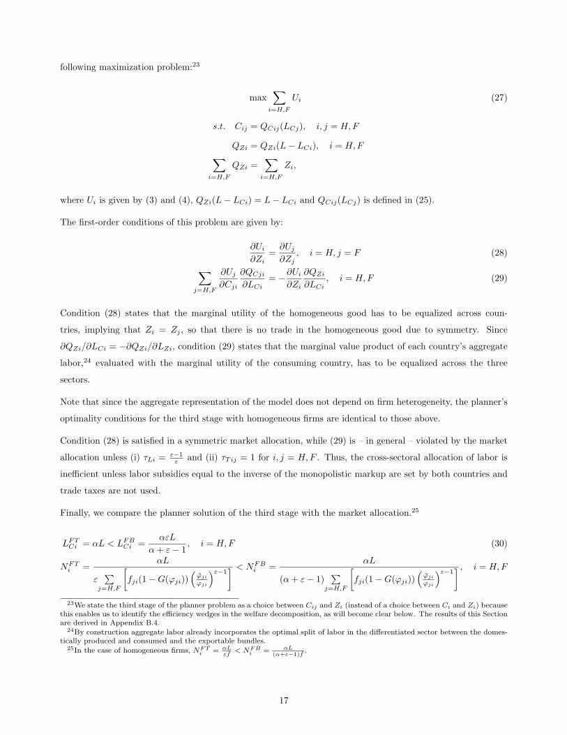
The first-order conditions of this problem are given by:

∂Ui

∂Zi=

∂Uj

∂Zj, i = H, j = F (28)

∑

j=H,F

∂Uj

∂Cji

∂QCji

∂LCi= −∂Ui

∂Zi

∂QZi

∂LCi, i = H,F (29)

Condition (28) states that the marginal utility of the homogeneous good has to be equalized across coun-

tries, implying that Zi = Zj , so that there is no trade in the homogeneous good due to symmetry. Since

∂QZi/∂LCi = −∂QZi/∂LZi, condition (29) states that the marginal value product of each country’s aggregate

labor,24 evaluated with the marginal utility of the consuming country, has to be equalized across the three

sectors.

Note that since the aggregate representation of the model does not depend on firm heterogeneity, the planner’s

optimality conditions for the third stage with homogeneous firms are identical to those above.

Condition (28) is satisfied in a symmetric market allocation, while (29) is – in general – violated by the market

allocation unless (i) τLi =ε−1ε and (ii) τTij = 1 for i, j = H,F . Thus, the cross-sectoral allocation of labor is

inefficient unless labor subsidies equal to the inverse of the monopolistic markup are set by both countries and

trade taxes are not used.

Finally, we compare the planner solution of the third stage with the market allocation.25

LFTCi = αL < LFB

Ci =αεL

α+ ε− 1, i = H,F (30)

NFTi =

αL

ε∑

j=H,F

[fji(1−G(ϕji))

(ϕji

ϕji

)ε−1] < NFB

i =αL

(α+ ε− 1)∑

j=H,F

[fji(1−G(ϕji))

(ϕji

ϕji

)ε−1] , i = H,F

23We state the third stage of the planner problem as a choice between Cij and Zi (instead of a choice between Ci and Zi) becausethis enables us to identify the efficiency wedges in the welfare decomposition, as will become clear below. The results of this Sectionare derived in Appendix B.4.

24By construction aggregate labor already incorporates the optimal split of labor in the differentiated sector between the domes-tically produced and consumed and the exportable bundles.

25In the case of homogeneous firms, NFTi = αL

εf< NFB

i = αL(α+ε−1)f

.

17

According to condition (30), the wedge in the marginal value product of labor between the homogeneous and the

differentiated sectors implies that the market allocates too little labor to the differentiated sector (LFTCi < LFB

Ci )

and thus provides too little variety (NFTi < NFB

i ). This reflects the fact that the monopolistic markup in the

differentiated sector depresses its relative demand.

3.4 Pareto efficiency and market equilibrium

The following Proposition summarizes all optimality conditions that need to be satisfied in order for the market

allocation to be Pareto optimal.

Proposition 1 Relationship between the planner and the market allocation

The market equilibrium coincides with the planner allocation if and only if:

(a)

∂ui

∂Cii

∂QCii

∂LCii=

∂uj

∂Cji

∂QCji

∂LCji, i, j = H,F i 6= j

(b) and (for the multi-sector model only)

∂Ui

∂Zi=

∂Uj

∂Zj, i = H, j = F

∑

j=H,F

∂Uj

∂Cji

∂QCji

∂LCi= −∂Ui

∂Zi

∂QZi

∂LCi, i = H,F

Proof See Appendix B.5.

Proposition 1 implies that the solution to the first stage of the planner problem always coincides with the

market allocation, so that the relative production of individual firms is optimal in any market equilibrium. By

contrast, for the market equilibrium to coincide with the solution to the second stage of the planner problem,

trade taxes cannot be operative because this would distort the consumption choice of the importable bundles.

Finally, the solution to the third stage of the planner problem (which is present only in the multi-sector model)

coincides with the market solution only when the amount of labor allocated across the differentiated sector is

efficient. This requires eliminating distortions from monopolistic markups with labor subsidies, as shown in the

next section.

4 The World Policy Maker Problem and the Welfare Decomposition

In the previous section we have derived the symmetric Pareto-efficient allocation chosen by the world planner

and have compared it with the market allocation. In this section, we solve the problem of the world policy maker

18

who maximizes the sum of individual-country welfare and has all three policy instruments (labor, import and

export taxes) at his disposal. We show that, by solving the world-policy-maker problem using a total-differential

approach, we can obtain a welfare decomposition that: (i) incorporates all general-equilibrium effects of setting

policy instruments under cooperation; (ii) and consequently allows separating policy makers’ incentives driven

by pure beggar-thy-neighbor motives from efficiency considerations.

The world policy maker sets domestic and foreign policy instruments τLi, τIi and τXi in order to solve the

following problem:

max

δji, ϕji, ϕji, Cji,Wi

Pij , LCi, τLi, τIi, τXii,j=H,F

∑

i=H,F

Ui (31)

subject to conditions (7)-(14).

where Ui is defined in (3), (4) and (15) with the additional restrictions that τT,i for i = H,F is as defined in

(6), Wi = 1 for i = H,F if α < 1 and that WF = 1 and LCi = L for i = H,F if α = 1.26

As a first step, solving the world policy maker problem using the total-differential approach involves taking total

differentials of (31) and the equilibrium equations. We then substitute the total differentials of the equilibrium

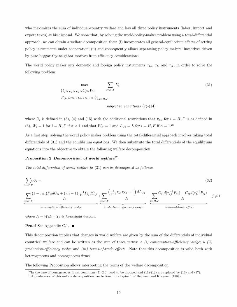
equations into the objective to obtain the following welfare decomposition:

Proposition 2 Decomposition of world welfare27

The total differential of world welfare in (31) can be decomposed as follows:

∑

i=H,F

dUi = (32)

∑

i=H,F

(1− τXi)PiidCii + (τIi − 1)τ−1Ii PijdCij

Ii︸︷︷︸

consumption- efficiency wedge

+∑

i=H,F

(ε

ε−1τLiτXi − 1)dLCi

Ii︸︷︷︸

production- efficiency wedge

+∑

i=H,F

Cjid(τ−1Ij Pji)− Cijd(τ

−1Ii Pij)

Ii︸︷︷︸

terms-of-trade effect

j 6= i

where Ii = WiL+ Ti is household income.

Proof See Appendix C.1.

This decomposition implies that changes in world welfare are given by the sum of the differentials of individual

countries’ welfare and can be written as the sum of three terms: a (i) consumption-efficiency wedge; a (ii)

production-efficiency wedge and (iii) terms-of-trade effects. Note that this decomposition is valid both with

heterogeneous and homogeneous firms.

The following Proposition allows interpreting the terms of the welfare decomposition.

26In the case of homogeneous firms, conditions (7)-(10) need to be dropped and (11)-(12) are replaced by (16) and (17).27A predecessor of this welfare decomposition can be found in chapter 1 of Helpman and Krugman (1989).

19

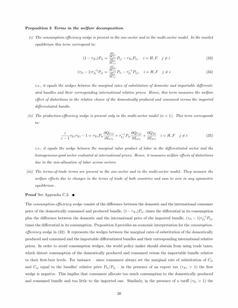
Proposition 3 Terms in the welfare decomposition

(i) The consumption-efficiency wedge is present in the one-sector and in the multi-sector model. In the market

equilibrium this term correspond to:

(1− τXi)Pii =∂Ui

∂Cii

∂Ui

∂Cij

Pij − τXiPii, i = H,F j 6= i (33)

(τIi − 1)τ−1Ii Pij =

∂Ui

∂Cij

∂Ui

∂Cii

Pii − τ−1Ii Pij , i = H,F j 6= i (34)

i.e., it equals the wedges between the marginal rates of substitution of domestic and importable differenti-

ated bundles and their corresponding international relative prices. Hence, this term measures the welfare

effect of distortions in the relative choice of the domestically produced and consumed versus the imported

differentiated bundle.

(ii) The production-efficiency wedge is present only in the multi-sector model (α < 1). This term corresponds

to:

ε

ε− 1τLiτXi − 1 = τXiPii

∂QCii

∂LCi+ τ−1

Ij Pji∂QCji

∂LCi+

∂QZi

∂LCii = H,F j 6= i (35)

i.e., it equals the wedge between the marginal value product of labor in the differentiated sector and the

homogeneous-good sector evaluated at international prices. Hence, it measures welfare effects of distortions

due to the mis-allocation of labor across sectors.

(iii) The terms-of-trade terms are present in the one-sector and in the multi-sector model. They measure the

welfare effects due to changes in the terms of trade of both countries and sum to zero in any symmetric

equilibrium .


The consumption-efficiency wedge consist of the difference between the domestic and the international consumer

price of the domestically consumed and produced bundle, (1− τXi)Pii, times the differential in its consumption

plus the difference between the domestic and the international price of the imported bundle, (τIi − 1)τ−1Ii Pij ,

times the differential in its consumption. Proposition 3 provides an economic interpretation for the consumption-

efficiency wedge in (32). It represents the wedges between the marginal rates of substitution of the domestically

produced and consumed and the importable differentiated bundles and their corresponding international relative

prices. In order to avoid consumption wedges, the world policy maker should abstain from using trade taxes,

which distort consumption of the domestically produced and consumed versus the importable bundle relative

to their first-best levels. For instance – since consumers always set the marginal rate of substitution of Cii

and Cij equal to the bundles’ relative price Pii/Pij – in the presence of an export tax (τXi > 1) the first

wedge is negative. This implies that consumers allocate too much consumption to the domestically produced

and consumed bundle and too little to the imported one. Similarly, in the presence of a tariff (τIi > 1) the

20

second wedge is positive, implying that the marginal rate of substitution of the importable and the domestically

produced and consumed bundle is larger than their international price τ−1Ii Pij . Thus, consumers allocate too

little consumption to the imported bundle and too much to the domestically produced one.

The production-efficiency wedge is present only in the case of multiple sectors (α < 1). It consists of the difference

between the international producer price of individual varieties and the international price of the homogeneous

good times the differential of labor allocated to the differentiated sector. According to Proposition 3, these terms

measure the difference of the marginal value product of labor between the differentiated and the homogeneous

sector. This term determines whether the allocation of labor across sectors is efficient. To guarantee production

efficiency, the world policy maker should set the labor subsidy τLi or the export subsidy τXi equal to the inverse

of the firms’ mark up, (ε− 1)/ε.

Finally, the terms-of-trade terms consist of the differentiated exportable bundle times the differential of its

international price minus the differentiated importable bundle times the differential of its international price.

An increase in the price of exportables raises domestic welfare and decreases welfare in the other country, while

an increase in the price of importables has the opposite effects. At the optimum the domestic and foreign terms-

of-trade effects exactly compensate each other, so that the differential of world welfare consists exclusively of

the consumption efficiency and the production efficiency terms.

Observe that the welfare decomposition in (32) holds independently of the number of instruments at the disposal

of the world policy maker. However, as made clear by the next Proposition, if the world policy maker can set

all three policy instruments at a time, setting all the terms in the welfare decomposition in (32) individually

equal to zero is in fact the solution to the policy problem in (31). It identifies the optimal coordinated policy

that implements the symmetric Pareto-efficient allocation as a market equilibrium.

Proposition 4 Optimal world policies and Pareto efficiency

When labor, import and export taxes are available,

(a) Solving the world-policy-maker problem in (31) by using the total-differential approach requires to set each

of the wedges in (32) equal to zero.

(b) As a result, under the optimal policy:

(i) τXi = 1 ⇐⇒∂Ui∂Cii∂Ui∂Cij

Pij = τXiPii and τIi = 1 ⇐⇒∂Ui∂Cij∂Ui∂Cii

Pii = τIiPij for i = H,F and j 6= i, i.e.,

the marginal rates of substitution of domestic and importable differentiated bundles are equal to their

corresponding international relative prices.

(ii) if α < 1, εε−1τLiτXi = 1 ⇐⇒ τXiPii

∂QCii

∂LCi+ τ−1

Ij Pji∂QCji

∂LCi= −∂QZi

∂LCifor i = H,F and j 6= i, i.e., the

marginal value product of labor in the differentiated sector is equal to the marginal value of product in

the homogeneous-good sector evaluated at international prices.

(iii) if α = 1, τXi = τIi = τLi = 1, i.e., in the one-sector model the free-trade allocation is optimal and if

α < 1, τXi = τIi = 1 and τLi =ε−1ε for i = H,F i.e., in the presence of multiple sectors the world

21

policy maker abstains from using trade taxes and uses the labor subsidy to offset the monopolistic

distortion in the differentiated sector.

(c) The world policy maker implements the planner allocation given that:

(i) by (b) (i) the second-stage wedge is closed, i.e.:

∂ui

∂Cii

∂QCii

∂LCii=

∂uj

∂Cji

∂QCji

∂LCji, i = H,F j 6= i

(ii) in the presence of multiple sectors by combining (b) (i) and (b) (ii) also the third-stage wedges are

closed, i.e.:

∂Ui

∂Zi=

∂Uj

∂Zj, i = H, j = F

∑

j=H,F

∂Uj

∂Cji

∂QCji

∂LCi= −∂Ui

∂Zi

∂QZi

∂LCi, i = H,F


The interpretation of Proposition 4 is straightforward. In the one-sector model changes in world welfare are

given exclusively by consumption efficiency wedges. Production efficiency is always guaranteed in any market

allocation of the one-sector model: the monopolistic markup does not induce any cross-sectoral distortions in the

allocation of labor because of inelastic labor supply. Note that for the case of heterogeneous firms implementing

consumption efficiency is enough to ensure that all productivity cutoffs ϕij are optimal, since this corresponds

to closing the gap between the marginal rate of substitution and transformation within the differentiated sector

in the second stage of the planner problem (equation (22)). This implies that the productivity cutoffs ϕij are

optimal in the free-trade allocation but are distorted whenever trade taxes are used. Consequently, LCi and

Ni are also efficient. Hence, for the case of the one-sector model the free-trade allocation coincides with the

planner allocation.

By contrast, in the market equilibrium of the multi-sector model, monopolistic markups do cause distortions in

the allocation of labor across sectors: the size of the differentiated sector is too small, whereas the size of the

homogeneous sector is too large. Consequently, the world policy maker can fully restore Pareto efficiency by

providing a labor subsidy to the differentiated sector. Again, implementing consumption efficiency is enough to

ensure that all productivity cutoffs ϕij are optimal. This implies that the productivity cutoffs ϕij are optimal

in the free-trade allocation but are distorted whenever trade taxes are used. Finally, it follows that only the

measure of firms that try to enter the differentiated sector, Ni, is too low in the free-trade allocation.

Proposition 4 confirms the message from the planner problem: achieving production and consumption efficiency

requires abstaining from the use of trade taxes and, in the case of the multi-sector model, offsetting markups by

subsidizing labor. Most importantly, a key result is contained in points (a) and (c) of Proposition 4: closing the

22

wedges in the welfare decomposition (32) one by one is a necessary and sufficient condition for implementing

the Pareto-efficient allocation, which is the allocation chosen by the world policy maker. This makes clear that

the welfare decomposition in (32) internalizes all the equilibrium constraints binding the world policy maker’s

optimal decisions in problem (31). For this reason, this decomposition incorporates all general equilibrium

effects and all relevant tradeoffs that the world policy maker faces when setting optimal policies. Finally, since

the world policy maker is concerned with implementing an efficient allocation, the terms in the above welfare

decomposition correspond unequivocally to consumption and production efficiency wedges.

5 Policy from the Individual Country Perspective

5.1 Individual Country Policy Maker Problem and the Welfare Decomposition

We now turn to the welfare incentives of policy makers that are concerned with maximizing the welfare of

individual countries and have either all policy instruments (labor and trade taxes) or a subset of them available.

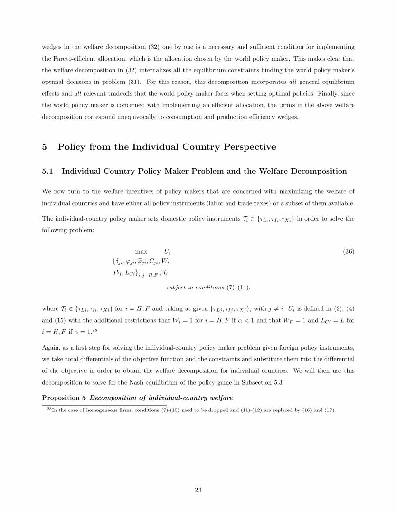
The individual-country policy maker sets domestic policy instruments Ti ∈ τLi, τIi, τXi in order to solve the

following problem:

max

δji, ϕji, ϕji, Cji,Wi

Pij , LCii,j=H,F , Ti

Ui (36)

subject to conditions (7)-(14).

where Ti ∈ τLi, τIi, τXi for i = H,F and taking as given τLj , τIj , τXj, with j 6= i. Ui is defined in (3), (4)

and (15) with the additional restrictions that Wi = 1 for i = H,F if α < 1 and that WF = 1 and LCi = L for

i = H,F if α = 1.28

Again, as a first step for solving the individual-country policy maker problem given foreign policy instruments,

we take total differentials of the objective function and the constraints and substitute them into the differential

of the objective in order to obtain the welfare decomposition for individual countries. We will then use this

decomposition to solve for the Nash equilibrium of the policy game in Subsection 5.3.

Proposition 5 Decomposition of individual-country welfare

28In the case of homogeneous firms, conditions (7)-(10) need to be dropped and (11)-(12) are replaced by (16) and (17).

23

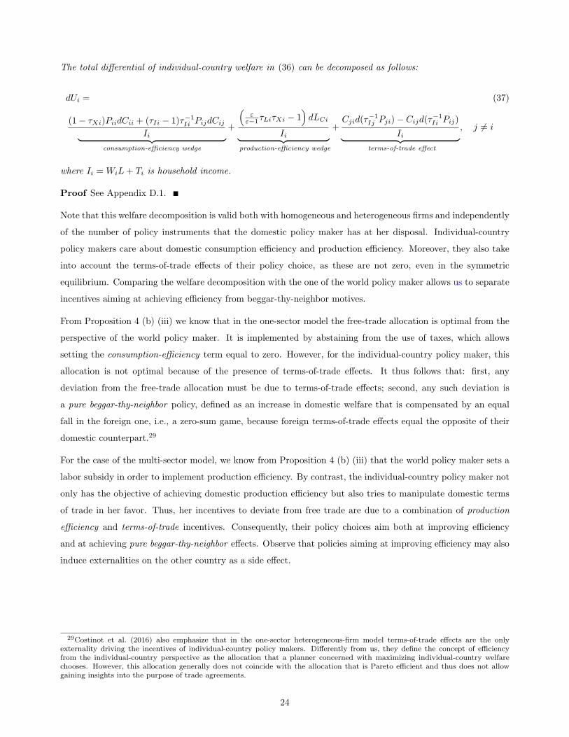
The total differential of individual-country welfare in (36) can be decomposed as follows:

dUi = (37)

(1− τXi)PiidCii + (τIi − 1)τ−1Ii PijdCij

Ii︸︷︷︸consumption-efficiency wedge

+

(ε

ε−1τLiτXi − 1)dLCi

Ii︸︷︷︸production-efficiency wedge

+Cjid(τ

−1Ij Pji)− Cijd(τ

−1Ii Pij)

Ii︸︷︷︸terms-of-trade effect

, j 6= i

where Ii = WiL+ Ti is household income.

Proof See Appendix D.1.

Note that this welfare decomposition is valid both with homogeneous and heterogeneous firms and independently

of the number of policy instruments that the domestic policy maker has at her disposal. Individual-country

policy makers care about domestic consumption efficiency and production efficiency. Moreover, they also take

into account the terms-of-trade effects of their policy choice, as these are not zero, even in the symmetric

equilibrium. Comparing the welfare decomposition with the one of the world policy maker allows us to separate

incentives aiming at achieving efficiency from beggar-thy-neighbor motives.

From Proposition 4 (b) (iii) we know that in the one-sector model the free-trade allocation is optimal from the

perspective of the world policy maker. It is implemented by abstaining from the use of taxes, which allows

setting the consumption-efficiency term equal to zero. However, for the individual-country policy maker, this

allocation is not optimal because of the presence of terms-of-trade effects. It thus follows that: first, any

deviation from the free-trade allocation must be due to terms-of-trade effects; second, any such deviation is

a pure beggar-thy-neighbor policy, defined as an increase in domestic welfare that is compensated by an equal

fall in the foreign one, i.e., a zero-sum game, because foreign terms-of-trade effects equal the opposite of their

domestic counterpart.29

For the case of the multi-sector model, we know from Proposition 4 (b) (iii) that the world policy maker sets a

labor subsidy in order to implement production efficiency. By contrast, the individual-country policy maker not

only has the objective of achieving domestic production efficiency but also tries to manipulate domestic terms

of trade in her favor. Thus, her incentives to deviate from free trade are due to a combination of production

efficiency and terms-of-trade incentives. Consequently, their policy choices aim both at improving efficiency

and at achieving pure beggar-thy-neighbor effects. Observe that policies aiming at improving efficiency may also

induce externalities on the other country as a side effect.

29Costinot et al. (2016) also emphasize that in the one-sector heterogeneous-firm model terms-of-trade effects are the onlyexternality driving the incentives of individual-country policy makers. Differently from us, they define the concept of efficiencyfrom the individual-country perspective as the allocation that a planner concerned with maximizing individual-country welfarechooses. However, this allocation generally does not coincide with the allocation that is Pareto efficient and thus does not allowgaining insights into the purpose of trade agreements.

24

The following Corollary summarizes these observations:

Corollary 1 Individual-country incentives

(a) In the one-sector model, any deviations of individual-country policy makers from free trade are due to

terms-of-trade effects.

(b) In the multi-sector model, individual-country policy makers’ deviations from free trade are driven by terms-

of-trade and production-efficiency effects.

(c) Terms-of-trade effects are the only pure beggar-thy-neighbor effects.

5.2 How Policy Instruments affect the Terms of Trade and Production Efficiency

Before studying strategic policies in Section 5.3, we first analyze how unilateral policy choices affect the terms of

trade and the efficiency wedges and thereby the welfare of individual countries. We are particularly interested in

explaining the different channels through which policy instruments impact on the terms of trade and efficiency.

As mentioned previously, the macro terms of trade can be influenced both through changes in the international

prices of individual exportable and importable varieties and through changes in the measure of exporters and

importers.

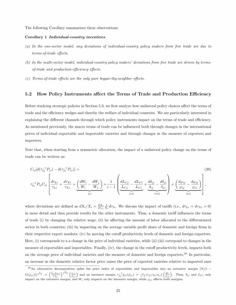
Note that, when starting from a symmetric allocation, the impact of a unilateral policy change on the terms of

trade can be written as:

Cij [d(τ−1Ij Pji)− d(τ−1

Ii Pij)] = (38)

τ−1Ii PijCij

dτLi

τLi+

dτXi

τXi+

(dWi

Wi− dWj

Wj

)

︸︷︷︸(i)

+1

ε− 1

dLCj

LCj− dLCi

LCi︸︷︷︸(ii)

+dδijδij

− dδjiδji︸︷︷︸

(iii)

+

(dϕij

ϕij− dϕji

ϕji

)

︸︷︷︸(iv)

,

where deviations are defined as dXi/Xi =∂Xi

∂τIi1Xi

dτIi. We discuss the impact of tariffs (i.e., dτLi = dτXi = 0)

in more detail and then provide results for the other instruments. Thus, a domestic tariff influences the terms

of trade (i) by changing the relative wage; (ii) by affecting the amount of labor allocated to the differentiated

sector in both countries; (iii) by impacting on the average variable profit share of domestic and foreign firms in

their respective export markets; (iv) by moving the cutoff productivity levels of domestic and foreign exporters.

Here, (i) corresponds to a a change in the price of individual varieties, while (ii)-(iii) correpond to changes in the

measure of exportables and importables. Finally, (iv), the change in the cutoff productivity levels, impacts both

on the average price of individual varieties and the measure of domestic and foreign exporters.30 In particular,

an increase in the domestic relative factor price raises the price of exported varieties relative to imported ones

30An alternative decomposition splits the price index of exportables and importables into an extensive margin [Ni(1 −

G(ϕji))]1

1−ε =(

δjiLCi

εfji

) 1ε−1

(

ϕji

ϕji

)

and an intensive margin τ−1Ij pji(ϕji) = ε

ε−1(τjiτXiτLi)

(

Wiϕji

)

. Thus, δji and LCi only

impact on the extensive margin, and Wi only impacts on the intensive margin, while ϕji affects both margins.

25

and improves the terms of trade. By contrast, an increase in the amount of labor allocated to the domestic

differentiated sector worsens the terms of trade by reducing the price index of exportables via an increase in

the number of varieties, while an increase in foreign labor allocated to the differentiated sector improves them

by reducing the price index of importables. Domestic terms of trade worsen with an increment in the average

variable-profit share of domestic firms from exports and improve in the foreign share by changing the measure

of firms that export to each market. Finally, an increase in the domestic cutoff-productivity level for exports

worsens the terms of trade both by making the average exportable variety cheaper and by affecting the measure

of exporters, whereas an increase in the foreign productivity cutoff has the opposite effect.

We first discuss the impact of a small unilateral tariff (i.e., dτLi = dτXi = 0) in the one-sector model (i.e.,

dLCj = dLCi = 0), starting from free trade. In the presence of a single sector, the terms-of-trade effects of a

small tariff are positive and given by31

PijCij

(dWi

Wi− dWj

Wj

)

︸︷︷︸(i)>0

+(ε− 1)−1

(dδijδij

− dδjiδji

)

︸︷︷︸(iii)>0

+

(dϕij

ϕij− dϕji

ϕji

)

︸︷︷︸(iv)<0

> 0 (39)

A tariff raises home’s demand for domestically produced varieties and thus, ceteris paribus, home firms’ profits

and the demand for domestic labor. Since labor supply is completely inelastic in the one-sector model, home’s

relative wage needs to adjust upward in response to a positive change in labor demand ((i)> 0), thereby reducing

equilibrium profits of domestic firms. Moreover, the increase in relative domestic income increases the share of

variable profits of firms from both countries made in home’s domestic market, which improves home’s terms of

trade ((iii)> 0). Finally, the increase in the relative domestic wage leads to tougher selection into exporting at

home and less selection in the other country, which negatively impacts on home’s terms of trade ((iv)< 0). In

the absence of firm heterogeneity the tariff exclusively raises home’s relative wage. Firm heterogeneity leads to

two additional and opposing effects: if heterogeneity mostly affects the variable-profit share from exports, terms

of trade respond more to tariffs compared to the case of homogeneous firms; by contrast, if selection effects are

large firm heterogeneity tends to reduce the response of the terms of trade by reducing the average price of

exported varieties relative to the one of imported varieties. Note also that in the one-sector model production

efficiency is always guaranteed, so the only incentive to deviate from free trade by setting a tariff is the positive

terms-of-trade effect.

Finally, we consider the impact of a unilateral export tax. Differently from a tariff, an export tax increases the

international price of individual varieties directly but reduces the demand for domestic labor and thus home’s

relative wage. In the presence of homogeneous firms, the first effect dominates leading to a terms-of-trade

improvement. By contrast, with heterogeneous firms the direct increase in the international price of individual

varieties is completely offset by a drop in home’s relative wage, while the impact on domestic and foreign

31In Appendix D.4 we sign the contribution of each component to the terms-of-trade effect for the one-sector model.

26

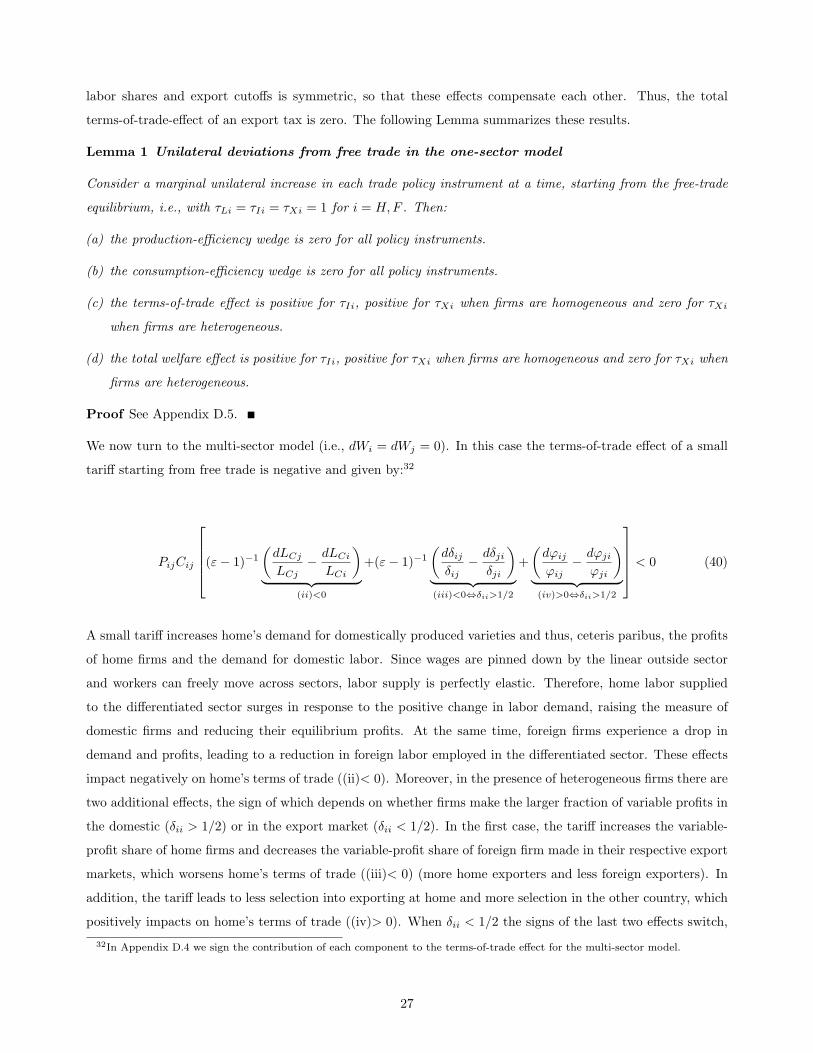
labor shares and export cutoffs is symmetric, so that these effects compensate each other. Thus, the total

terms-of-trade-effect of an export tax is zero. The following Lemma summarizes these results.

Lemma 1 Unilateral deviations from free trade in the one-sector model

Consider a marginal unilateral increase in each trade policy instrument at a time, starting from the free-trade

equilibrium, i.e., with τLi = τIi = τXi = 1 for i = H,F . Then:

(a) the production-efficiency wedge is zero for all policy instruments.

(b) the consumption-efficiency wedge is zero for all policy instruments.

(c) the terms-of-trade effect is positive for τIi, positive for τXi when firms are homogeneous and zero for τXi

when firms are heterogeneous.

(d) the total welfare effect is positive for τIi, positive for τXi when firms are homogeneous and zero for τXi when

firms are heterogeneous.


We now turn to the multi-sector model (i.e., dWi = dWj = 0). In this case the terms-of-trade effect of a small

tariff starting from free trade is negative and given by:32

PijCij

(ε− 1)−1

(dLCj

LCj− dLCi

LCi

)

︸︷︷︸(ii)<0

+(ε− 1)−1

(dδijδij

− dδjiδji

)

︸︷︷︸(iii)<0⇔δii>1/2

+

(dϕij

ϕij− dϕji

ϕji

)

︸︷︷︸(iv)>0⇔δii>1/2

< 0 (40)

A small tariff increases home’s demand for domestically produced varieties and thus, ceteris paribus, the profits

of home firms and the demand for domestic labor. Since wages are pinned down by the linear outside sector

and workers can freely move across sectors, labor supply is perfectly elastic. Therefore, home labor supplied

to the differentiated sector surges in response to the positive change in labor demand, raising the measure of

domestic firms and reducing their equilibrium profits. At the same time, foreign firms experience a drop in

demand and profits, leading to a reduction in foreign labor employed in the differentiated sector. These effects

impact negatively on home’s terms of trade ((ii)< 0). Moreover, in the presence of heterogeneous firms there are

two additional effects, the sign of which depends on whether firms make the larger fraction of variable profits in

the domestic (δii > 1/2) or in the export market (δii < 1/2). In the first case, the tariff increases the variable-

profit share of home firms and decreases the variable-profit share of foreign firm made in their respective export

markets, which worsens home’s terms of trade ((iii)< 0) (more home exporters and less foreign exporters). In

addition, the tariff leads to less selection into exporting at home and more selection in the other country, which

positively impacts on home’s terms of trade ((iv)> 0). When δii < 1/2 the signs of the last two effects switch,

32In Appendix D.4 we sign the contribution of each component to the terms-of-trade effect for the multi-sector model.

27

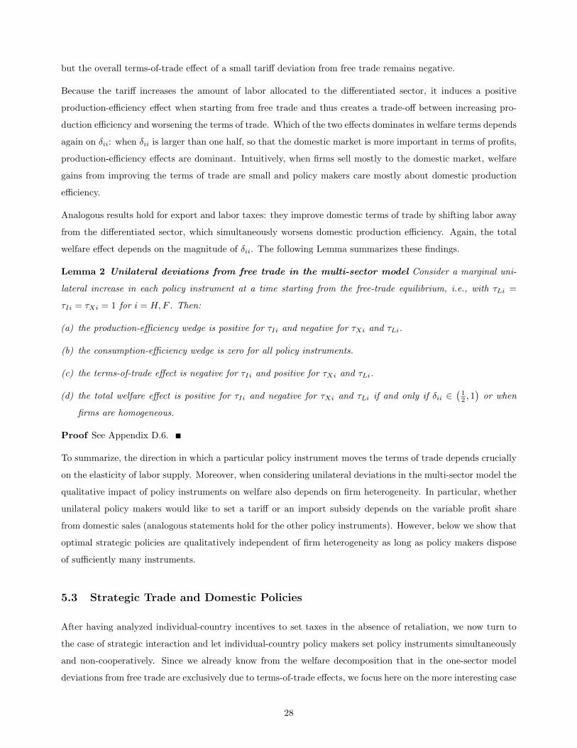
but the overall terms-of-trade effect of a small tariff deviation from free trade remains negative.

Because the tariff increases the amount of labor allocated to the differentiated sector, it induces a positive

production-efficiency effect when starting from free trade and thus creates a trade-off between increasing pro-

duction efficiency and worsening the terms of trade. Which of the two effects dominates in welfare terms depends

again on δii: when δii is larger than one half, so that the domestic market is more important in terms of profits,

production-efficiency effects are dominant. Intuitively, when firms sell mostly to the domestic market, welfare

gains from improving the terms of trade are small and policy makers care mostly about domestic production

efficiency.

Analogous results hold for export and labor taxes: they improve domestic terms of trade by shifting labor away

from the differentiated sector, which simultaneously worsens domestic production efficiency. Again, the total

welfare effect depends on the magnitude of δii. The following Lemma summarizes these findings.

Lemma 2 Unilateral deviations from free trade in the multi-sector model Consider a marginal uni-

lateral increase in each policy instrument at a time starting from the free-trade equilibrium, i.e., with τLi =

τIi = τXi = 1 for i = H,F . Then:

(a) the production-efficiency wedge is positive for τIi and negative for τXi and τLi.

(b) the consumption-efficiency wedge is zero for all policy instruments.

(c) the terms-of-trade effect is negative for τIi and positive for τXi and τLi.

(d) the total welfare effect is positive for τIi and negative for τXi and τLi if and only if δii ∈(12 , 1)or when

firms are homogeneous.


To summarize, the direction in which a particular policy instrument moves the terms of trade depends crucially

on the elasticity of labor supply. Moreover, when considering unilateral deviations in the multi-sector model the

qualitative impact of policy instruments on welfare also depends on firm heterogeneity. In particular, whether

unilateral policy makers would like to set a tariff or an import subsidy depends on the variable profit share

from domestic sales (analogous statements hold for the other policy instruments). However, below we show that

optimal strategic policies are qualitatively independent of firm heterogeneity as long as policy makers dispose

of sufficiently many instruments.

5.3 Strategic Trade and Domestic Policies

After having analyzed individual-country incentives to set taxes in the absence of retaliation, we now turn to

the case of strategic interaction and let individual-country policy makers set policy instruments simultaneously

and non-cooperatively. Since we already know from the welfare decomposition that in the one-sector model

deviations from free trade are exclusively due to terms-of-trade effects, we focus here on the more interesting case

28

of the multi-sector model, where both production-efficiency and terms-of-trade motives are present. Moreover,

for the moment we allow both domestic policies τLi and trade policies τIi, τXi, for i = H,F to be used.

Individual-country policy makers solve the problem described in (36). Similarly to the world policy maker

problem, the welfare decomposition in (37) holds independently of the number of instruments at the disposal

of the individual-country policy maker and corresponds to the policy maker’s objective. After substituting

additional equilibrium conditions, it can be written in terms of three terms that are individually equal to zero

at the optimum. Proposition 6 states this more formally and characterizes the symmetric Nash equilibrium.

Proposition 6 Strategic trade and domestic policies

When labor, import and export taxes are available,

(a) It is possible to rewrite (37) as follows:

dUi =1

Ii[ΩCiidCii +ΩCijdCij +ΩLCidLCi]

where ΩCii, ΩCij and ΩLCi are defined in Appendix D.2.

(b) Solving the individual-country policy maker problem in (36) by using the total-differential approach requires

setting ΩCii = ΩCij = ΩLCi = 0.

(c) As a result, any symmetric Nash equilibrium in the multi-sector model with homogeneous or heterogeneous

firms when both countries can simultaneously set all policy instruments entails the first-best level of labor

subsidies, and inefficient import subsidies and export taxes. Formally,

τNashL = ε−1

ε , τNashI < 1 and τNash

X > 1.

Proof See Appendix D.7

Our welfare decomposition allow us to interpret the Nash policy outcome stated in Proposition 6. Domestic

policies are set efficiently even under strategic interaction and do not cause any beggar-thy-neighbor effects, while

trade policy instruments are used to try to manipulate the terms of trade. As made clear by the discussion in the

last sub-section, an import subsidy or an export tax both aim at improving the terms of trade. Consequently,

even in the presence of domestic policies terms-of-trade externalities remain the only motive for signing a trade

agreement. Proposition 6 extends the result of Campolmi et al. (2014) – who find that in the two-sector

model with homogeneous firms strategic trade policy consists of first-best labor subsidies and inefficient import

subsidies and export taxes – to the case of heterogeneous firms.

The result that labor subsidies are set so as to completely offset monopolistic distortions is an application of

the targeting principle in public economics (Dixit, 1985). It states that an externality or distortion is best

countered with a tax instrument that acts directly on the appropriate margin. If the policy maker disposes

of sufficiently many instruments to deal with each incentive separately, she uses the labor subsidy to address

production efficiency. The trade policy instruments are instead used to exploit the terms-of-trade effect, which

29

is the only remaining incentive according to our welfare decomposition. Because there are two relative prices

(the one of the differentiated exportable bundle and the one of the differentiated imporable bundle relative to

the homogeneous good) two trade-policy instruments are necessary to target both.

This result implies that firm heterogeneity neither adds further motives for signing a trade agreement beyond

the classical terms-of-trade effect nor changes the qualitative results (import subsidies and export taxes) of the

equilibrium outcome compared to the case with homogeneous firms. This finding is different from the unilateral

case (Lemma 2), where the welfare effects of unilateral deviations in trade taxes depend on parameter values,

as summarized by the share of variable profits from domestic sales. It also differs from the results of Costinot et

al. (2016), who find in a slightly more general model that the optimal unilateral policy may not only be affected

quantitatively but also qualitatively by firm heterogeneity.

Our finding that domestic policies do not introduce new motives for trade policy coordination is closely related

to the conclusion of Bagwell and Staiger (1999) and Bagwell and Staiger (2016), who uncover that in a large

class of economic models terms-of-trade motives are the only reason for signing a trade agreement.Proposition 6

extends their result (i) to models with monopolistic competition and heterogeneous firms; and (ii) the presence

of domestic policies.

Finally, we turn to the optimal design of trade agreements from the perspective of monopolistic competition

models. Again, we focus on the multi-sector model, which features a clear motive for domestic policies.33

Obviously, implementation of the first-best allocation requires a trade agreement that includes cooperation

on both trade and domestic policies (see Proposition 4). However, most trade agreements – in particular,

GATT-WTO – do not regulate domestic policies to the extent that they do not imply outright discrimination

of foreign goods.34 We therefore consider a situation where domestic policy is set non-cooperatively in the

presence of a trade agreement that prevents countries from choosing trade policy instruments strategically. For

simplicity, we focus on the case of full trade liberalization, as required, e.g. by a regional trade agreement under

Article 24 of GATT-WTO, but one can also think of a multilateral agreement that prevents countries from

using trade instruments strategically, such as GATT- WTO.35 In the case where only domestic policies can be

set strategically, individual-country policy makers face a missing-instrument problem and there is a trade off

between increasing production efficiency (calling for a labor subsidy) and improving the terms of trade (calling

for a labor tax). Thus, it is ex ante unclear which motive dominates in equilibrium and one has to characterize

the Nash-equilibrium policies.

33In the one-sector model the free-trade allocation is Pareto optimal and individual-country policy makers’ only incentive is tomanipulate their terms of trade. Thus, the use of any type of policy instruments (both trade and labor taxes) should be restrictedby a trade agreement.

34 GATT Article III (1): The contracting parties recognize that internal taxes and other internal charges, and laws, regulationsand requirements affecting the internal sale, offering for sale, purchase, transportation, distribution or use of products, and internalquantitative regulations requiring the mixture, processing or use of products in specified amounts or proportions, should not beapplied to imported or domestic products so as to afford protection to domestic production. (...) (8 b) The provisions of this Articleshall not prevent the payment of subsidies exclusively to domestic producers, including payments to domestic producers derivedfrom the proceeds of internal taxes or charges applied consistently with the provisions of this Article and subsidies effected throughgovernmental purchases of domestic products.

35GATT-WTO features tariff bindings and prohibition of export taxes.

30

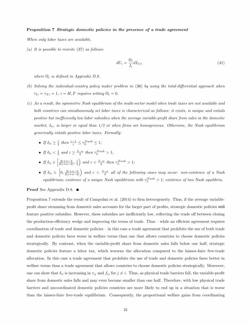
Proposition 7 Strategic domestic policies in the presence of a trade agreement

When only labor taxes are available,

(a) It is possible to rewrite (37) as follows:

dUi =Ωi

IidLCi (41)

where Ωi is defined in Appendix D.8.

(b) Solving the individual-country policy maker problem in (36) by using the total-differential approach when

τIi = τXi = 1, i = H,F requires setting Ωi = 0.

(c) As a result, the symmetric Nash equilibrium of the multi-sector model when trade taxes are not available and

both countries can simultaneously set labor taxes is characterized as follows: it exists, is unique and entails

positive but inefficiently low labor subsidies when the average variable-profit share from sales in the domestic

market, δii, is larger or equal than 1/2 or when firms are homogeneous. Otherwise, the Nash equilibrium

generically entails positive labor taxes. Formally:

• If δii ≥ 12 then ε−1

ε ≤ τNashL ≤ 1;

• If δii <12 and ε ≥ 3−α

2 then τNashL > 1;

• If δii ∈[

2ε+α−32(ε+α−2) ,

12

)and ε < 3−α

2 then τNashL > 1;

• If δii ∈[0, 2ε+α−3

2(ε+α−2)

)and ε < 3−α

2 all of the following cases may occur: non-existence of a Nash

equilibrium; existence of a unique Nash equilibrium with τNashL > 1; existence of two Nash equilibria.


Proposition 7 extends the result of Campolmi et al. (2014) to firm heterogeneity. Thus, if the average variable-

profit share stemming from domestic sales accounts for the larger part of profits, strategic domestic policies still

feature positive subsidies. However, these subsidies are inefficiently low, reflecting the trade off between closing

the production-efficiency wedge and improving the terms of trade. Thus – while an efficient agreement requires

coordination of trade and domestic policies – in this case a trade agreement that prohibits the use of both trade

and domestic policies fares worse in welfare terms than one that allows countries to choose domestic policies

strategically. By contrast, when the variable-profit share from domestic sales falls below one half, strategic

domestic policies feature a labor tax, which worsens the allocation compared to the laissez-faire free-trade

allocation. In this case a trade agreement that prohibits the use of trade and domestic policies fares better in

welfare terms than a trade agreement that allows countries to choose domestic policies strategically. Moreover,

one can show that δii is increasing in τij and fij for j 6= i. Thus, as physical trade barriers fall, the variable-profit

share from domestic sales falls and may even become smaller than one half. Therefore, with low physical trade

barriers and uncoordinated domestic policies countries are more likely to end up in a situation that is worse

than the laissez-faire free-trade equilibrium. Consequently, the proportional welfare gains from coordinating

31

domestic policies in the presence of a trade agreement rise as physical trade barriers fall. These insights on the

welfare effects of trade agreements are summarized by the following Proposition and the associated Corollary.

Proposition 8 Welfare effects of strategic domestic policies in the presence of a trade agreement

Assume that τIi = τXi = 1 for i = H,F and let the average variable-profit share from sales in the domestic

market be given by δii.

(a) When δii ≥ 12 or in the presence of homogeneous firms, the symmetric Nash equilibrium when countries can

only set domestic policies strategically welfare-dominates the laisez-faire free-trade allocation with τLi = 1,

i = H,F .

(b) When δii <12 the symmetric Nash equilibrium when countries can only set domestic policies strategically is

welfare-dominated by the free-trade allocation with τLi = 1, i = H,F .

(c) δii is increasing in τij and fij, j 6= i.


Corollary 2 The design of trade agreements in the presence of domestic policies

(a) Implementing the first-best allocation requires a joint agreement on trade and domestic policies.

(b) When δii ≥ 12 or in the presence of homogeneous firms, an agreement that forbids the strategic use of trade

policies and allows countries to set domestic policies freely welfare dominates an agreement that forbids

countries to use domestic and trade policies.

(c) When δii <12 an agreement that forbids countries to use domestic and trade policies welfare dominates an

agreement that forbids the strategic use of trade policies and allows countries to set domestic policies freely.

(d) The proportional welfare gains from a joint agreement on trade and domestic policies compared to an agree-

ment that only prohibits trade taxes but allows countries to set domestic policies freely are larger when

physical trade barriers are small compared to when they are large.

6 Conclusion

Trade models with monopolistic competition and heterogeneous firm (Melitz, 2003) have become the workhorse

for positive analysis in trade theory. Surprisingly, so far relatively little research has been dedicated to the

normative implications of this framework. In particular, the question which international externalities are solved

by trade agreements in multi-sector models with heterogeneous firms and how to design trade agreements from

their perspective has so far not been addressed by the literature. This is reflected in the review article by

Bagwell and Staiger (2016), who limit their discussion of the design of trade agreements to homogeneous-firm

models.

32

In this paper we have made progress on several fronts. Starting with the observation that trade models with

CES preferences and monopolistic competition have a common macro representation, we have shown that this

class of models also has common welfare incentives for trade and domestic policies. Solving the problem of a

world policy maker, we have derived a welfare decomposition that decomposes world welfare changes induced by

trade and domestic policies into changes in consumption wedges and production wedges. As long as the world

policy maker disposes of a sufficient set of instruments, she closes these wedges one by one and implements

the first-best allocation. In the multi-sector model this requires using labor subsidies to offset monopolistic

markups.

From the individual-country perspective, welfare incentives for trade and domestic policies are additionally

governed by terms-of-trade incentives. This makes clear that terms-of-trade effects are the only pure beggar-

thy-neighbor externality in this class of models.

Then we have discussed how individual policy instruments affect the terms of trade. We have shown that

firm heterogeneity matters here in two respects: first, through selection into exporting, by affecting the cutoff

productivity of exporters; second, via the impact on the variable-profit share arising from sales in each market.

Finally, we have studied strategic trade and domestic policies within the multi-sector heterogeneous-firm model.

We have shown that when all policy instruments can be set strategically, the Nash equilibrium entails the

first-best level of labor subsidies and inefficient import subsidies and export taxes that aim at improving the

terms of trade. This result is qualitatively independent of firm heterogeneity. Thus, even in the presence of firm

heterogeneity and domestic policies terms-of-trade motives remain the only reason for signing a trade agreement.

Moreover, when a trade agreement prevents countries from use trade policy strategically, domestic policies are

set to balance a trade off between improving the terms of trade and increasing production efficiency. Nash-

equilibrium domestic policies – and thus, whether the strategic use of domestic policies should be proscribed by

a trade agreement – depends on the variable profit-share on domestic sales. When this number is larger than

one half, the Nash equilibrium features positive (albeit inefficiently low) labor subsidies. By contrast, when this

number is smaller than one half, the Nash equilibrium is characterized by positive labor taxes.

To conclude we point out some limitations of our work and discuss directions for future research. The main

restriction of the CES framework with monopolistic competition is that markups are constant and independent

of the level of competition. Empirically, markups tend to be higher for more productive firms and pass through

is incomplete (Hottman, Redding and Weinstein, 2016). Relaxing the constant-markup assumption requires

either to dispense of CES preferences or to introduce oligopolistic firms (Atkeson and Burstein, 2012). See

Bagwell and Lee (2015) for an analysis of strategic trade policy in monopolistic competition models with linear

demand. In the presence of variable markups achieving production efficiency necessitates firm-specific subsidies

and in their absence policy makers operate in a second-best environment. A further potential extension of our

study is to analyze optimal trade and domestic policies in the presence of trade in intermediate inputs and

global production chains. Here, Blanchard, Bown and Johnson (2017) provide some first insights.

33

References

Arkolakis, Costas, Arnaud Costinot, and Andres Rodrıguez-Clare, “New Trade Models, Same Old

Gains?,” American Economic Review, 2012, 102 (1), 94–130.

Atkeson, Andrew and Ariel Burstein, “Pricing-to-market, Trade Costs, and International Relative Prices,”

American Economic Review, 2012, 98 (5), 1998–2031.

Bagwell, Kyle and Robert W. Staiger, “An Economic Theory of GATT,” American Economic Review,

1999, 89 (1), 215–248.

and , “Chapter 8 - The Design of Trade Agreements,” in Kyle Bagwell and Robert W. Staiger, eds.,

Handbook of Commercial Policy, Vol. 1A, Elsevier, 2016.

and Seun Hoon Lee, “Trade Policy under Monopolistic Competition and Firm Selection,” mimeo, 2015.

Blanchard, Emily, Chad Bown, and Robert Johnson, “Global Supply Chains and Trade Policy,” mimeo,

2017.

Campolmi, Alessia, Harald Fadinger, and Chiara Forlati, “Trade Policy: Home Market Versus Terms

of Trade Externality,” Center for Fiscal Policy Working Paper, 2012.

, , and , “Trade Policy: Home Market Versus Terms of Trade Externality,” Journal of International

Economics, 2014, 93, 92–107.

Copeland, Brian R., “Strategic Interaction among Nations: Negotiable and Non-negotiable Trade Barriers,”

Canadian Journal of Economics, 1990, 21 (1), 84–108.

Costinot, Arnaud, Andres Rodrıguez-Clare, and Ivan Werning, “Micro to Macro: Optimal Trade

Policy with Firm Heterogeneity,” mimeo, 2016.

Demidova, Svetlana and Andres Rodrıguez-Clare, “Trade Policy Under Firm-level Heterogeneity in a

Small Open Economy,” Journal of International Economics, 2009, 78, 100–112.

Dhingra, Swati and John Morrow, “Monopolistic Competition and Optimum Product Diversity under

Firm Heterogeneity,” Journal of Political Economy, 2019, forthcoming.

Dixit, Avinash K., “Tax policy in Open Economies,” in Allan. J. Auerbach and Martin Feldstein, eds.,

Handbook of Public Economics, Vol. 1, Elsevier, 1985.

Ederington, Josh, “International Coordination of Trade and Domestic Policies,” American Economic Review,

2001, 91 (5), 1580–1593.

Felbermayr, Gabriel, Benjamin Jung, and Mario Larch, “Optimal Tariffs, Retaliation, and the Welfare

Loss from Tariff Wars in the Melitz Model,” Journal of International Economics, 2013, 89, 13–25.

34

Gros, Daniel, “A Note on the Optimal Tariff Retaliation and the Welfare Loss from Tariff Wars in a Framework

with Intra-Industry Trade,” Journal of International Economics, 1987, 23 (3-4), 357–367.

Haaland, Jan I. and Anthony J. Venables, “Optimal Trade Policy with Monopolistic Competition and

Heterogeneous Firms,” Journal of International Economics, 2016, 102, 85–95.

Helpman, Elhanan and Paul Krugman, Trade Policy and Market Structure, MIT Press, 1989.

Hottman, Collin, Stephen Redding, and David Weinstein, “Quantifying the Sources of Firm Hetero-

geneity,” Quarterly Journal of Economics, 2016, 131 (3), 1291–1364.

Krugman, Paul, “Scale Economics, Product Differentiation, and Pattern of Trade,” American Economic

Review, 1980, 70 (5), 950–959.

Melitz, Marc J., “The Impact of Trade on Intra-Industry Reallocations and Aggregate Industry Productivity,”

Econometrica, 2003, 71 (6), 1695–1725.

and Stephen J. Redding, “Heterogeneous Firms and Trade,” in Elhanan Helpman Gita Gopinath and

Kenneth Rogoff, eds., Handbook of International Economics, Vol. 4, Elsevier, 2015.

Ossa, Ralph, “A ’New Trade’ Theory of GATT/WTO Negotiations,” Journal of Political Economy, 2011, 119

(1), 122–152.

Venables, Anthony, “Trade and Trade Policy with Differentiated Products: A Chamberlinian-Ricardian

Model,” The Economic Journal, 1987, 97 (387), 700–717.

35

APPENDIX

A The Model

A.1 Households

Given the Dixit-Stiglitz structure of preferences in (4), the households’ maximization problem can be solved inthree stages. At the first two stages, households choose how much to consume of each domestically producedand foreign produced variety, and how to allocate consumption between the domestic and the foreign bundles.The optimality conditions imply the following demand functions and price indices:

cij(ϕ) =

[pij(ϕ)

Pij

]−ε

Cij , Cij =

[Pij

Pi

]−ε

Ci, i, j = H,F (A-1)

Pi =

∑

j∈H,F

P 1−εij

11−ε

, Pij =

[Nj

∫ ∞

ϕij

pij(ϕ)1−εdG(ϕ)

] 11−ε

, i, j = H,F (A-2)

Here Pi is the price index of the differentiated bundle in country i, Pij is the country-i price index of thebundle of differentiated varieties produced in country j, and pij(ϕ) is the country-i consumer price of variety ϕproduced by country j.

In the last stage, households choose how to allocate consumption between the homogeneous good and thedifferentiated bundle. Thus, they maximize (3) subject to the following budget constraint:

PiCi + pZiZi = Ii, i = H,F

where Ii = WiL+Ti is total income and Ti is a lump sum transfer which depends on the tax scheme adopted bythe country-i government. The solution to the consumer problem implies that the marginal rate of substitutionbetween the homogeneous good and the differentiated bundle equals their relative price:

α

1− α

Zi

Ci=

Pi

pZi, i = H,F (A-3)

Then following Melitz and Redding (2015), we can rewrite the demand functions as

cij(ϕ) = pij(ϕ)−εAi, Cij = P−ε

ij Ai, Ci = P−εi Ai, i = H,F, (A-4)

where Ai ≡ P ε−1i αIi. Ai can be interpreted as an index of market (aggregate) demand.

A.2 Firms

A.2.1 Firms’ behavior in the differentiated sector

Given the constant price elasticity of demand, optimal prices charged by country-i firms in their domesticmarket are a fixed markup over their perceived marginal cost (τLi

Wi

ϕ ), and optimal prices charged to country-jconsumers for varieties produced in country i equal country-i prices augmented by transport costs and tradetaxes

pji(ϕ) = τjiτTjiτLiε

ε− 1

Wi

ϕ, i, j = H,F (A-5)

The optimal pricing rule implies the following firm revenues:

rji(ϕ) ≡ τ−1Tjipji(ϕ)cji(ϕ) = τ−1

Tjipji(ϕ)1−εAj = ετ1−ε

ji τ−εTjiτ

1−εLi W 1−ε

i ϕε−1Bj , i = H,F, (A-6)

36

where Bi ≡(

εε−1

)1−ε1εAi. Profits are given by:

πji(ϕ) ≡ Bj

(τLiWi

ϕ

)1−ε

τ1−εji τ−ε

Tji − τLiWifji =rji(ϕ)

ε− τLiWifji, i = H,F (A-7)

A.2.2 Zero-profit conditions

Firms choose to produce for the domestic (export) market only when this is profitable. Since profits aremonotonically increasing in ϕ, we can determine the equilibrium productivity cutoffs for firms active in thedomestic market and export market, ϕji, by setting πji(ϕji) = 0, namely:

πji(ϕji) = 0 ⇒ rji(ϕji)

ε= τLiWifji (A-8)

As in Melitz (2003), we call these conditions the zero profit (ZCP) conditions. Using (A-7) we rewrite (A-8) asfollows:

Bj = τ ε−1ji τ εLiτ

εTjiW

εi ϕ

1−εji i, j = H,F (A-9)

A.2.3 Free-entry conditions (FE)

The free entry (FE) conditions require expected profits (before firms know the realization of their productivity)in each country to be zero in equilibrium:

∑

j∈H,F

∫ ∞

ϕji

πji(ϕ)dG(ϕ) = τLiWifE

Substituting optimal profits (A-7), we obtain

∑

j∈H,F

∫ ∞

ϕji

[Bj

(τLiWi

ϕ

)1−ε

τ1−εji τ−ε

Tji − τLiWifji

]dG(ϕ) = τLiWifE (A-10)

A.2.4 Firms’ behavior in the homogeneous sector

Since the homogeneous good is sold in a perfectly competitive market without trade costs, price equals marginalcost and is the same in both countries. We assume that the homogeneous good is produced in both countriesin equilibrium. Given the production technology, this implies factor price equalization in the presence of thehomogeneous sector:

pZi = pZj = Wi = Wj = 1

A.3 Government

The government is assumed to run a balanced budget. Hence, country-i government’s budget constraint is givenby:

Ti = (τIi − 1)τ−1Ii PijCij + (τXi − 1)τ−1

TjiPjiCji+

+ (τLi − 1)NiWi

∑

k=H,F

∫ ∞

ϕki

(qki(ϕ)

ϕ+ fki

)dG(ϕ) + fE

i = H,F j 6= i

37

Government income consists of import tax revenues charged on imports of differentiated goods gross of transportcosts and foreign export taxes (thus, tariffs are charged on CIF values of foreign exports), export tax revenuescharged on exports gross of transport costs, and labor tax revenues.

A.4 Equilibrium

Substituting ZCP (A-9) into FE (A-10), we obtain:

∑

j=H,F

fji(1−G(ϕji))

(ϕji

ϕji

)ε−1

= fE +∑

j=H,F

fji(1−G(ϕji)) i = H,F, (A-11)

where

ϕji =

[∫ ∞

ϕji

ϕε−1 dG(ϕ)

1−G(ϕji)

] 1ε−1

, i, j = H,F, (A-12)

which correspond to (10) and (7) in the main text. Moreover, dividing the ZCP conditions (A-9), we obtaincondition (9) in the main text:

(ϕii

ϕij

)=

(fiifij

) 1ε−1(τLi

τLj

) εε−1(Wi

Wj

) εε−1

τ−1ij τ

− εε−1

Tij i, j = H,F (A-13)

The remaining equilibrium equations are then given as follows:

Consumption sub-indices which can be determined using (A-4) jointly with (A-9):

Cij = P−εij

(ε

ε− 1

)ε−1

ετ εCjτε−1ij τ εT ijϕ

1−εij W ε

j fij , i, j = H,F (A-14)

Price sub-indices which emerge from substituting (A-5) into (A-2):

P 1−εij =

(ε

ε− 1

)1−ε

Nj(1−G(ϕij))(τijτTijτLj)1−εϕε−1

ij W 1−εj , i, j = H,F (A-15)

Aggregate profits Πi are given by Πi = Ri − τLiWiLCi + τLiWiNifE , where Ri are aggregate revenues,Ri ≡ Ni

∑j=H,F

∫∞

ϕjirji(ϕ)dG(ϕ). From the FE condition (A-10) it then follows that Πi = τLiWiNifE

and thus Ri = τLiWiLCi. Substituting the definition of optimal revenues (A-6) into the previous condition,we get

τLiWiLCi = εNi

∑

j=H,F

∫ ∞

ϕji

Bjτ1−εji τ−ε

Tjiτ1−εLi W 1−ε

i ϕε−1dG(ϕ)

Combining this condition with (10) and (A-9), we obtain:

Labor market clearing in the differentiated sector

LCi = εNi

∑

j=H,F

fji(1−G(ϕji)) + εfENi i = H,F (A-16)

This can be solved for the equilibrium level of Ni:

38

Ni =LCi

ε∑

j=H,F fji(1−G(ϕji)) + εfEi = H,F (A-17)

Combining this last condition with (10), plugging into (A-14) and (A-15) and taking into account thedefinition (7) allow us to recover (11) and (12) in the main text.

In the presence of the homogeneous sector, the trade-balance condition is given by:36

(QZi − Zi) + τ−1Ij PjiCji = τ−1

Ii PijCij i = H, j = F

The left-hand side of this equation is the sum of the net export value of the homogeneous goods andthe value of the differentiated exportable bundle (at CIF inclusive international prices), while the right-hand side is the value of the differentiated importable bundle (at CIF inclusive international prices). Inthe absence of the homogeneous sector the first term is zero and we can use this condition directly. Bycontrast, in presence of this sector, we can use the fact that

∑j=H,F PijCij = PiCi to rewrite (A-3) as:

Zi =(1− α)

α

∑

j=H,F

PijCij i = H,F (A-18)

We can combine this equation with the trade-balance condition above and the aggregate labor marketclearing L = LCi + LZi to obtain:

Trade-balance condition

L− LCi −(1− α)

α

∑

k=H,F

PikCik + τ−1Ij PjiCji = τ−1

Ii PijCij , i = H, j = F, (A-19)

which corresponds to condition (13).

Finally, when the homogeneous sector is present, we also require equilibrium in the market for the ho-mogenous good, i.e.

∑i=H,F QZi =

∑i=H,F Zi. Combining this condition with aggregate labor market

clearing and demand for the homogeneous good (A-3) we obtain:

Homogeneous good market clearing condition

∑

i=H,F

(L− LCi) =1− α

α

∑

i=H,F

∑

j=H,F

PijCij , (A-20)

which coincides with condition (14).

A.5 From Melitz to Krugman (1980)

In this section we show how the equilibrium equations (7) to (15) need to be modified to obtain the Krugman(1980) model.

To obtain the Krugman (1980) model with homogeneous firms, the following assumptions are needed:

1. Let fij = 0 for i, j = H,F (there are no fixed market access costs).

2. Let G(ϕ) be degenerate at unity.

3. Conditions (7), (8) (9) and (10) need to be dropped from the set of equilibrium conditions.

36Import taxes are collected directly by the governments at the border so they do not enter into this condition.

39

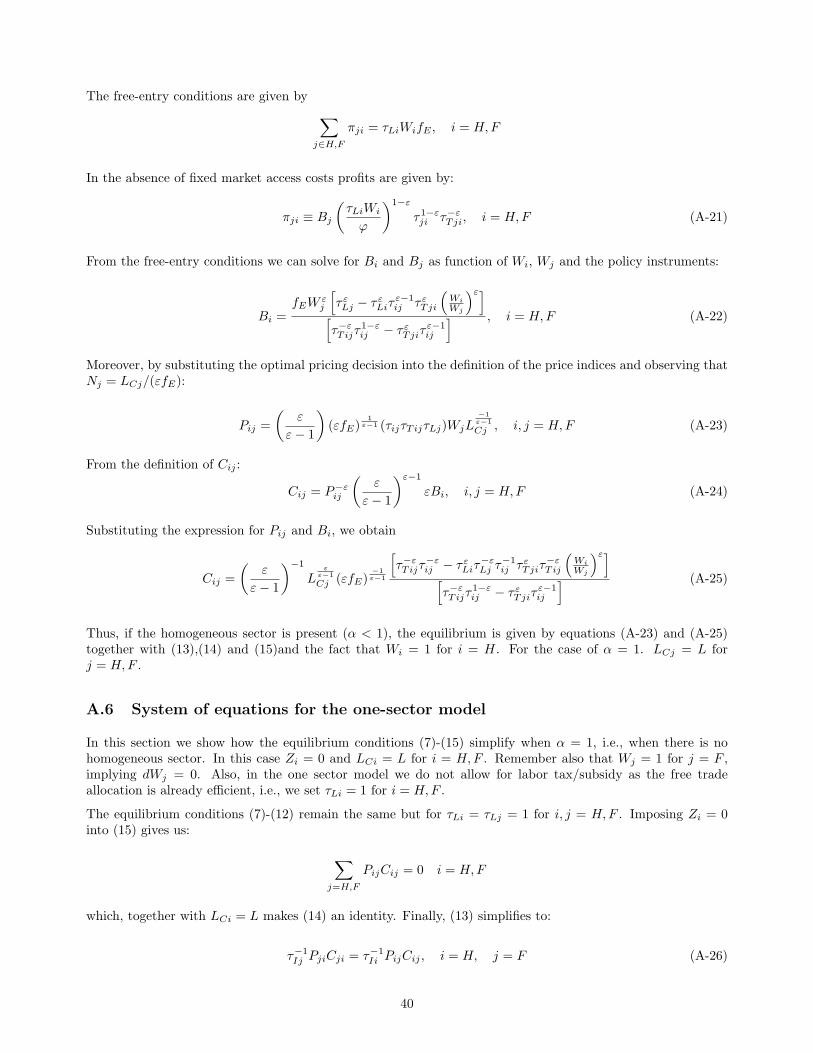
The free-entry conditions are given by

∑

j∈H,F

πji = τLiWifE , i = H,F

In the absence of fixed market access costs profits are given by:

πji ≡ Bj

(τLiWi

ϕ

)1−ε

τ1−εji τ−ε

Tji, i = H,F (A-21)

From the free-entry conditions we can solve for Bi and Bj as function of Wi, Wj and the policy instruments:

Bi =fEW

εj

[τ εLj − τ εLiτ

ε−1ij τ εTji

(Wi

Wj

)ε]

[τ−εT ijτ


ε−1ij

] , i = H,F (A-22)

Moreover, by substituting the optimal pricing decision into the definition of the price indices and observing thatNj = LCj/(εfE):

Pij =

(ε

ε− 1

)(εfE)

1ε−1 (τijτTijτLj)WjL

−1ε−1

Cj , i, j = H,F (A-23)

From the definition of Cij :

Cij = P−εij

(ε

ε− 1

)ε−1

εBi, i, j = H,F (A-24)

Substituting the expression for Pij and Bi, we obtain

Cij =

(ε

ε− 1

)−1

Lε

ε−1

Cj (εfE)−1ε−1

[τ−εT ijτ

−εij − τ εLiτ

−εLj τ

−1ij τ εTjiτ

−εT ij

(Wi

Wj

)ε]

[τ−εT ijτ


ε−1ij

] (A-25)

Thus, if the homogeneous sector is present (α < 1), the equilibrium is given by equations (A-23) and (A-25)together with (13),(14) and (15)and the fact that Wi = 1 for i = H. For the case of α = 1. LCj = L forj = H,F .

A.6 System of equations for the one-sector model

In this section we show how the equilibrium conditions (7)-(15) simplify when α = 1, i.e., when there is nohomogeneous sector. In this case Zi = 0 and LCi = L for i = H,F . Remember also that Wj = 1 for j = F ,implying dWj = 0. Also, in the one sector model we do not allow for labor tax/subsidy as the free tradeallocation is already efficient, i.e., we set τLi = 1 for i = H,F .

The equilibrium conditions (7)-(12) remain the same but for τLi = τLj = 1 for i, j = H,F . Imposing Zi = 0into (15) gives us:

∑

j=H,F

PijCij = 0 i = H,F

which, together with LCi = L makes (14) an identity. Finally, (13) simplifies to:

τ−1Ij PjiCji = τ−1

Ii PijCij , i = H, j = F (A-26)

40

A.7 Solving for the free-trade allocation

Using equations (11) and (12), we find that

PijCij = δijLCjτTijτLjWj , i, j = H,F (A-27)

Substituting into the trade-balance condition (13), we obtain:

L− LCi −(1− α)

α

∑

k=H,F

δikLCkτTikτLkWk + δjiLCiτXiτLiWi = δijLCjτXjτLjWj , i = H, j = F (A-28)

In the free-trade allocation, τLi = τIi = τXi = 1 for i = H,F . Since the countries are symmetric, the equilibriumis also symmetric and thus LCi = LCj , Wi = Wj = 1, δij = δji for i, j = H,F .

Substituting these conditions, we find that

LFTCi = αL, i = H,F (A-29)

Using this result together with (A-16) and (A-11), we obtain

NFTi =

αL

ε∑

j=H,F

[fji(1−G(ϕji))

(ϕji

ϕji

)ε−1] , i = H,F (A-30)

A.8 Total differentials of the equilibrium equations

Since total differentials of the equilibrium equations are extensively used in the proofs, we present them herefor future reference.

The total differential of (7) gives:

dϕji =1

ε− 1

g(ϕji)

[1−G(ϕji)]ϕji

[1−

(ϕji

ϕji

)ε−1]dϕji, i, j = H,F (A-31)

Taking the total differential of (10) and using (A-31) we get:

dϕji = − fii[1−G(ϕii)]ϕ−εii ϕε−1

ii

fji[1−G(ϕji)]ϕ−εji ϕ

ε−1ji

dϕii, i, j = H,F, i 6= j (A-32)

Using the definition of δii obtained by combining (8) with (10), this can also be written in a more compact way:

dϕji = − δii1− δii

ϕji

ϕiidϕii (A-33)

Combining (8) with (10), taking the total differential, and using (A-31) and (A-32), we get:

dδji = − δjiϕji

(Φi + (ε− 1)) dϕji, i, j = H,F (A-34)

where Φi ≡ δiig(ϕji)ϕ

εjiϕ

1−εji

1−G(ϕji)+ δji

g(ϕii)ϕεiiϕ

1−εii

1−G(ϕii)> 0, i = H,F .

41

Taking the total differential of (11) we obtain:

dϕij =ϕij

CijdCij −

ε

ε− 1

ϕij

δijdδij −

ε

ε− 1

ϕij

LCjdLCj , i, j = H,F (A-35)

which, using the symmetric condition of (A-34) to substitute out dδij , becomes:

dϕij =εϕij

LCj(ε− 1)(ε− 1 + ε

ε−1Φj

)dLCj −ϕij

Cij

(ε− 1 + ε

ε−1Φj

)dCij , i, j = H,F (A-36)

For future use, we substitute the symmetric condition of (A-36) into (A-34):

dδji =δji(ε− 1 + Φi)

Cji

(ε− 1 + ε

ε−1Φi

)dCji −δjiε(ε− 1 + Φi)

LCi(ε− 1)(ε− 1 + ε

ε−1Φi

)dLCi, i, j = H,F (A-37)

Taking the total differential of (9), we have:

dϕij =ϕij

ϕiidϕii +

ε

ε− 1ϕij

[dτLj

τLj− dτLi

τLi+

dWj

Wj− dWi

Wi+

dτTij

τTij

], i, j = H,F, i 6= j (A-38)

where dτTji = 0 if i = j while dτTji = τXidτIj + τIjdτXi if i 6= j.

B The Planner Allocation

In this Appendix, we derive the main results of Section 3. First, we set up the planner problem and solve itusing a three-stage approach. Finally, we prove Proposition 1.

B.1 The Planner Problem

The full planner problem can be written as follows. The planner maximizes:

∑

i=H,F

Ui =∑

i=H,F

∑

j=H,F

Cε−1ε

ij

εαε−1

Z1−αi

with respect to Cij ,LCij , Zi, Ni, cij(ϕ), lij(ϕ), ϕij , for i, j = H,F and subject to:

Cij =

[Nj

∫ ∞

ϕij

cij(ϕ)ε−1ε dG(ϕ)

] εε−1

, i, j = H,F

lij(ϕ) =τijcij(ϕ)

ϕ+ fij , i, j = H,F

LCij = Nj

∫ ∞

ϕij

lij(ϕ)dG(ϕ), i, j = H,F

LCi = NifE +∑

j=H,F

LCji, i, j = H,F

∑

i=H,F

Li =∑

i=H,F

LCi +∑

i=H,F

Zi

42

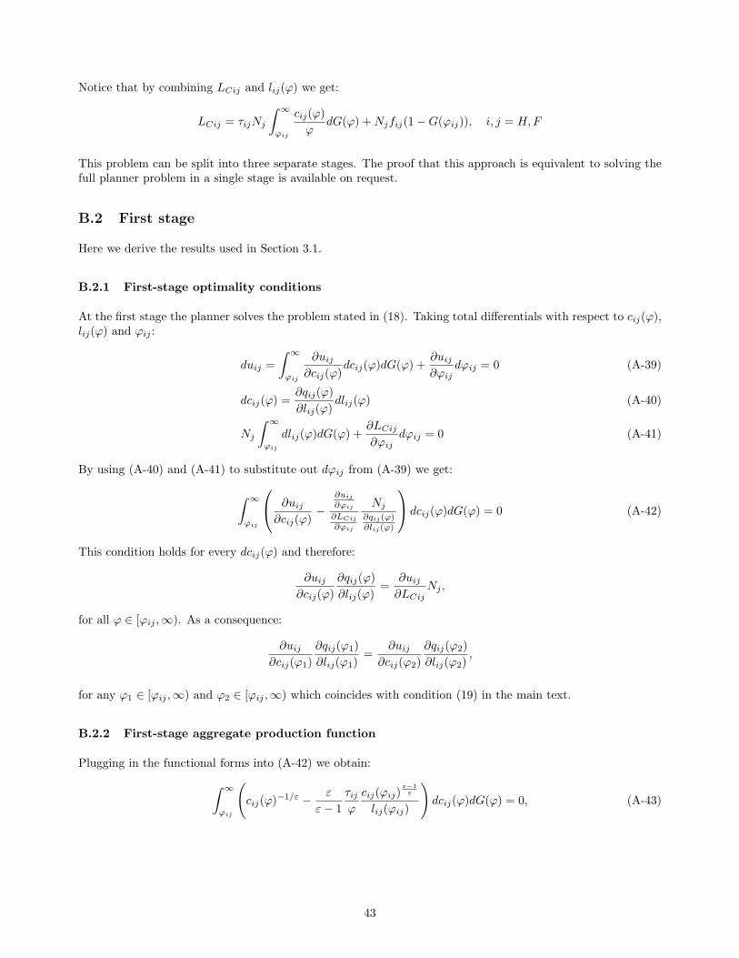
Notice that by combining LCij and lij(ϕ) we get:

LCij = τijNj

∫ ∞

ϕij

cij(ϕ)

ϕdG(ϕ) +Njfij(1−G(ϕij)), i, j = H,F

This problem can be split into three separate stages. The proof that this approach is equivalent to solving thefull planner problem in a single stage is available on request.

B.2 First stage

Here we derive the results used in Section 3.1.

B.2.1 First-stage optimality conditions

At the first stage the planner solves the problem stated in (18). Taking total differentials with respect to cij(ϕ),lij(ϕ) and ϕij :

duij =

∫ ∞

ϕij

∂uij

∂cij(ϕ)dcij(ϕ)dG(ϕ) +

∂uij

∂ϕijdϕij = 0 (A-39)

dcij(ϕ) =∂qij(ϕ)

∂lij(ϕ)dlij(ϕ) (A-40)

Nj

∫ ∞

ϕij

dlij(ϕ)dG(ϕ) +∂LCij

∂ϕijdϕij = 0 (A-41)

By using (A-40) and (A-41) to substitute out dϕij from (A-39) we get:

∫ ∞

ϕij

∂uij

∂cij(ϕ)−

∂uij

∂ϕij

∂LCij

∂ϕij

Nj

∂qij(ϕ)∂lij(ϕ)

dcij(ϕ)dG(ϕ) = 0 (A-42)

This condition holds for every dcij(ϕ) and therefore:

∂uij

∂cij(ϕ)

∂qij(ϕ)

∂lij(ϕ)=

∂uij

∂LCijNj ,

for all ϕ ∈ [ϕij ,∞). As a consequence:

∂uij

∂cij(ϕ1)

∂qij(ϕ1)

∂lij(ϕ1)=

∂uij

∂cij(ϕ2)

∂qij(ϕ2)

∂lij(ϕ2),

for any ϕ1 ∈ [ϕij ,∞) and ϕ2 ∈ [ϕij ,∞) which coincides with condition (19) in the main text.

B.2.2 First-stage aggregate production function

Plugging in the functional forms into (A-42) we obtain:

∫ ∞

ϕij

(cij(ϕ)

−1/ε − ε

ε− 1

τijϕ

cij(ϕij)ε−1ε

lij(ϕij)

)dcij(ϕ)dG(ϕ) = 0, (A-43)

43

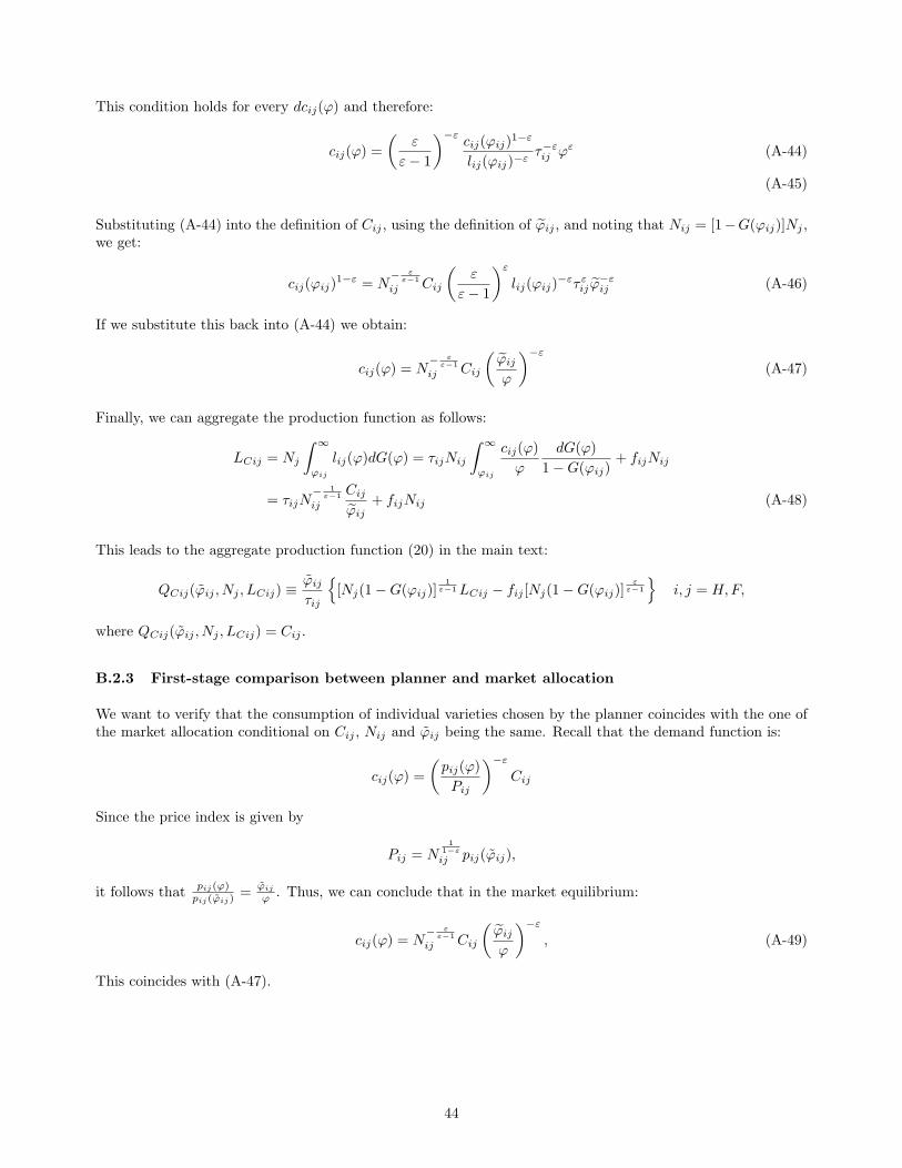
This condition holds for every dcij(ϕ) and therefore:

cij(ϕ) =

(ε

ε− 1

)−εcij(ϕij)

1−ε

lij(ϕij)−ετ−εij ϕε (A-44)

(A-45)

Substituting (A-44) into the definition of Cij , using the definition of ϕij , and noting that Nij = [1−G(ϕij)]Nj ,we get:

cij(ϕij)1−ε = N

− εε−1

ij Cij

(ε

ε− 1

)ε

lij(ϕij)−ετ εijϕ

−εij (A-46)

If we substitute this back into (A-44) we obtain:

cij(ϕ) = N− ε

ε−1

ij Cij

(ϕij

ϕ

)−ε

(A-47)

Finally, we can aggregate the production function as follows:

LCij = Nj

∫ ∞

ϕij

lij(ϕ)dG(ϕ) = τijNij

∫ ∞

ϕij

cij(ϕ)

ϕ

dG(ϕ)

1−G(ϕij)+ fijNij

= τijN− 1

ε−1

ij

Cij

ϕij+ fijNij (A-48)

This leads to the aggregate production function (20) in the main text:

QCij(ϕij , Nj , LCij) ≡ϕij

τij

[Nj(1−G(ϕij)]

1ε−1LCij − fij [Nj(1−G(ϕij)]

εε−1

i, j = H,F,

where QCij(ϕij , Nj , LCij) = Cij .

B.2.3 First-stage comparison between planner and market allocation

We want to verify that the consumption of individual varieties chosen by the planner coincides with the one ofthe market allocation conditional on Cij , Nij and ϕij being the same. Recall that the demand function is:

cij(ϕ) =

(pij(ϕ)

Pij

)−ε

Cij

Since the price index is given by

Pij = N1

1−ε

ij pij(ϕij),

it follows thatpij(ϕ)pij(ϕij)

=ϕij

ϕ . Thus, we can conclude that in the market equilibrium:

cij(ϕ) = N− ε

ε−1

ij Cij

(ϕij

ϕ

)−ε

, (A-49)

This coincides with (A-47).

44

B.2.4 First stage with homogeneous firms

In this case the problem stated in (18) simplifies to choosing cij(ω) and lij(ω) for i, j = H,F by solving thefollowing problem:

maxuij (A-50)

s.t. cij(ω) = qij(ω), i, j = H,F

LCij =

∫ Nj

0

lij(ω)dω, i, j = H,F,

where uij ≡ Cij , Cij =[∫ Nj

0cij(ω)

ε−1ε dω

] εε−1

, qij(ω) = lij(ω)1τij

, and Nj and LCij are taken as given since

they are determined at the second stage. Solving this problem gives back the same condition condition withderived with heterogeneous firms:

∂uij

∂cij(ω1)

∂qij(ω1)

∂lij(ω1)=

∂uij

∂cij(ω2)

∂qij(ω2)

∂lij(ω2)

This implies that all firms will employ the same quantity of labor and produce the same amount of consumptiongood, i.e., lij(ω) = lij and cij(ω) = cij∀ω ∈ [0, Nj ]. Following the same steps as with heterogeneous firms wecan derive the aggregate level of consumption:

Cij = Nε

ε−1

j cij ,

which coincides with the market equilibrium (A-49). Finally, the aggregate production now simplifies to:

Cij =ϕ

τijN

1ε−1

j LCij

B.3 Second Stage

Here we derive the results of Section 3.2.

B.3.1 Second-stage optimality conditions and aggregate production function

At the second stage the planner solves the problem described in (21). Taking total differentials:

∑

i=H,F

∑

j=H,F

∂ui

∂CijdCij = 0

dNi = − 1

fE

∑

j=H,F

dLCji, i = H,F

dCij =∂QCij

∂NjdNj +

∂QCij

∂ϕijdϕij +

∂QCij

∂LCijdLCij , i, j = H,F

Substituting the differentials of the constraints into the objective, we obtain:

∑

i=H,F

∑

j=H,F

∂ui

∂Cij

∂QCij

∂ϕijdϕij +

∂QCij

∂LCijdLCij −

∂QCij

∂Nj

1

fE

∑

k=H,F

dLCkj

= 0

45

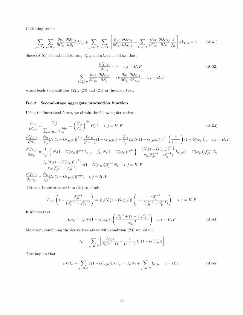
Collecting terms:

∑

j=H,F

∑

i=H,F

∂ui

∂Cij

∂QCij

∂ϕijdϕij +

∑

j=H,F

∑

i=H,F

∂ui

∂Cij

∂QCij

∂LCij−∑

k=H,F

∂uk

∂Ckj

∂QCkj

∂Nj

1

fE

dLCij = 0 (A-51)

Since (A-51) should hold for any dϕij and dLCij it follows that:

∂QCij

∂ϕij= 0, i, j = H,F (A-52)

∑

k=H,F

∂uk

∂Ckj

∂QCkj

∂Nj= fE

∂ui

∂Cij

∂QCij

∂LCij, i, j = H,F,

which leads to conditions (22), (23) and (24) in the main text.

B.3.2 Second-stage aggregate production function

Using the functional forms, we obtain the following derivatives:

∂ui

∂Cij=

C−1ε

ij

∑k=H,F C

ε−1ε

ik

=

(Cij

Ci

)−1ε

C−1i , i, j = H,F (A-53)

∂QCji

∂Ni=

ϕij

τij[Ni(1−G(ϕji))]

2−εε−1

LCji

(ε− 1)(1−G(ϕji))−

ϕji

τjifji[Ni(1−G(ϕji))]

1ε−1

(ε

ε− 1

)(1−G(ϕji)), i, j = H,F

∂QCji

∂ϕji=

1

τji

[Ni(1−G(ϕji)]

1ε−1LCji − fji[Ni(1−G(ϕji)]

εε−1

− [Ni(1−G(ϕji)]

2−εε−1

τji(ϕε−1ji − ϕε−1

ij )LCji(1−G(ϕji))ϕ

ε−1ji Ni

+fji[Ni(1−G(ϕji))]

1ε−1

τji(ϕε−1ji − ϕε−1

ji )ε(1−G(ϕji))ϕ

ε−1ji Ni, i, j = H,F

∂QCji

∂LCji=

ϕji

τji[Ni(1−G(ϕji))]

1ε−1 , i, j = H,F

This can be substituted into (24) to obtain:

LCji

(1−

ϕε−1ji

(ϕε−1ji − ϕε−1

ji )

)= fji[Ni(1−G(ϕji))]

(1−

εϕε−1ji

(ϕε−1ji − ϕε−1

ji )

), i, j = H,F

It follows that:

LCji = fjiNi(1−G(ϕji))

(ϕε−1ji + (ε− 1)ϕε−1

ji

ϕε−1ji

)i, j = H,F (A-54)

Moreover, combining the derivatives above with condition (23) we obtain:

fE =∑

j=H,F

[LCji

Ni(ε− 1)− ε

(ε− 1)fji(1−G(ϕji))

]

This implies that

εNifE +∑

j=H,F

ε(1−G(ϕji))Nifji = fENi +∑

j=H,F

LCji, i = H,F. (A-55)

46

Using (A-54) and LCi = fENi +∑

j=H,F LCji to substitute out LCji and fENi in (A-55), we find:

LCi =∑

j=H,F

εfjiNi(1−G(ϕji))

(ϕji

ϕji

)ε−1

, i = H,F

We use this last condition to solve for Ni:

Ni =LCi

ε∑

j=H,F

[fji(1−G(ϕji))

(ϕji

ϕji

)ε−1] , i = H,F (A-56)

We now substitute (A-54) and (A-64) into the definition (20) to obtain (25) in the main text.

B.3.3 Second-stage comparison between planner and market allocation

Next, we check if the optimality conditions of the second stage are satisfied in the market allocation.

First, consider condition (22). Plugging the relevant derivatives in (A-53), we obtain:

1

Ci

(Cii

Ci

)−1ε ϕii

τii[Ni(1−G(ϕii)]

1ε−1 =

1

Cj

(Cji

Cj

)−1ε ϕji

τji[Ni(1−G(ϕji)]

1ε−1 , i = H,F, j 6= i

Now consider the market allocation. Using (8) jointly with (9), (11) and (A-17) after some manipulations weget:

1

Ci

(Cii

Ci

)−1ε ϕii

τii[Ni(1−G(ϕii)]

1ε−1 =

1

Cj

(Cji

Cj

)−1ε ϕji

τji[Ni(1−G(ϕji)]

1ε−1

(Cj

Ci

τjiτii

ϕii

ϕji

) ε−1ε(fiifji

)−1ε

,i = H,F, j 6= i

Thus, in the market allocation:

∂ui

∂Cii

∂QCii

∂LCii= ΩP2

∂uj

∂Cji

∂QCji

∂LCji, i = H,F, j 6= i,

where ΩP2 is the wedge between the planner and the market allocation. Under symmetry:

ΩP2 =

(τjiτii

ϕii

ϕji

) ε−1ε(fiifji

)−1ε

, i = H,F, j 6= i

Using condition (9), this can be written as ΩP2 = τ−1Tij . This leads to condition (26).

Next, consider the planner’s optimality condition (23). Using the functional forms from (A-53), this correspondsto (see (A-55)):

fE =∑

j=H,F

LCjiN1−εi − fji(1−G(ϕji))

ε

ε− 1(A-57)

We now want to check if this condition is also fulfilled by the market allocation. Recalling the labor marketclearing condition in (A-16) and that LCi =

∑j=H,F LCji +NifE , we obtain condition (A-57) and this proves

that (23) is satisfied in any market allocation.

Finally, consider the planner’s optimality condition (24). As shown in Section B.3.2, this condition can berewritten as (A-54). Now consider the market allocation. Appendix B.2.3 shows that condition (A-47) holds inthe market equilibrium. As a consequence, also condition (A-48) holds in the market equilibrium. We can thenuse (A-48) and substitute it in equation (11) to obtain (A-54). This confirms that this condition and then (24)always holds both in the planner and in the market allocation.

47

B.3.4 Second stage with homogeneous firms

In this case the problem stated in (21) simplifies to choosing Cij , LCij , Ni for i, j = H,F in order to solve:

max∑

i=H,F

ui (A-58)

s.t. LCi = NifE +∑

j=H,F

LCji, i = H,F

Cij = QCij(Nj , LCij), i, j = H,F,

The first-order conditions of this problem are given by:

∂ui

∂Cii

∂QCii

∂LCii=

∂uj

∂Cji

∂QCji

∂LCji, i, j = H,F, i 6= j (A-59)

fE =∑

j=H,F

∂QCji/∂Ni

∂QCji/∂LCi, i = H,F (A-60)

B.3.5 Second-stage aggregate production function with homogeneous firms

Using the functional forms, we obtain the following derivatives:

∂ui

∂Cij=

C−1ε

ij

∑k=H,F C

ε−1ε

ik

=

(Cij

Ci

)−1ε

C−1i , i, j = H,F (A-61)

∂QCji

∂Ni=

ϕ

τijN

2−εε−1

i

LCji

(ε− 1), i, j = H,F

∂QCji

∂LCji=

ϕ

τjiN

1ε−1

i , i, j = H,F

Substituting the functional forms into (A-59), we obtain:

Cji = τ−εij

(Ci

Cj

)ε−1

Cii, i, j = H,F (A-62)

and

fE =∑

j=H,F

[LCji

Ni(ε− 1)

], i = H,F (A-63)

Using (A-54) and LCi = fENi +∑

j=H,F LCji to substitute out LCji and fENi in (A-55), we find:

Ni =LCi

εfE, i = H,F (A-64)

We can then substitute the production function Cji = LjiN1

ε−1

i τ−1ji into (A-62) to get:

LCji = τ1−εji

(Ci

Cj

)ε−1

LCii, i = H,F, j 6= i (A-65)

48

Substituting this into the labor market clearing LCi = LCii + LCji + NifE and using the definition of Ni =LCi/(εfE), we find that:

LCii = LCi

(ε− 1

ε

)[1 + τ1−ε

ij

(Ci

Cj

)ε−1]−1

, i = H,F (A-66)

LCji = τ1−εji

(Ci

Cj

)ε−1

LCi

(ε− 1

ε

)[1 + τ1−ε

ij

(Ci

Cj

)ε−1]−1

, i = H,F, j 6= i (A-67)

Using again the definition of the aggregate production function, we get

Cij =

(ε− 1

ε

)τ−εij (εfE)

−1ε−1L

εε−1

Cj

(Cj

Ci

)ε−1[1 + τ1−ε

ij

(Cj

Ci

)ε−1]−1

i = H,F, j 6= i. (A-68)

B.3.6 Second-stage comparison between planner and market allocation with homogeneous firms

Next, we check if the optimality conditions of the second stage are satisfied in the market allocation.

First, consider condition (A-62), which can be written as:

1

Ci

(Cii

Ci

)−1ε

=1

Cj

(Cji

Cj

)−1ε 1

τji, i = H,F, j 6= i

Now consider the market allocation. From the demand functions we get

Cii

Cji=

(Pii

Pji

)−ε(Ci

Cj

)1−ε(PiCi

PjCj

)ε

, i = H,F, j 6= i

This can also be written as:

1

Ci

(Cii

Ci

)−1ε

=1

Cj

(Cji

Cj

)−1ε 1

τjiτji

(Pii

Pji

)(PjCj

PiCi

), i = H,F, j 6= i

In other words, in the market allocation:

∂ui

∂Cii

∂QCii

∂LCii=

∂uj

∂Cji

∂QCji

∂LCjiΩP2, i = H,F, j 6= i

where ΩP2 ≡ τji

(Pii

Pji

)(PjCj

PiCi

)is the wedge between the planner and the market allocation. Under symmetry

ΩP2 = τ−1Tji.

Next, consider the planner’s optimality condition (A-63):

fE =∑

j=H,F

LCji

Ni(ε− 1), i = H,F (A-69)

We now want to check if this condition is also fulfilled in the market allocation. Recalling the labor marketclearing requires LCi = εfENi and that LCi =

∑j=H,F LCji+NifE , we obtain condition (A-69) and this proves

that (A-63) is satisfied in any market allocation.

49

B.4 Third stage

Here we derive the results from Section 3.3.

B.4.1 Third-stage optimality conditions

In the third stage, the planner chooses Cij , Zi and LCi for i, j = H,F to solve the maximization problem in(27). Taking total differentials of the objective function and of the constraints, we get:

∑

i=H,F

dUi =∑

i=H,F

∑

j=H,F

∂Ui

∂CijdCij +

∑

i=H,F

∂Ui

∂ZidZi

dCij =∂QCij

∂LCjdLCj , i, j = H,F

dQZi =∂QZi

∂LCidLCi, i = H,F

∑

i=H,F

dQZi =∑

i=H,F

dZi

Substituting the total differential of the constraints into the total differential of the objective and rearranging:

∑

k=H,F

dUk =∑

k=H,F

∑

l=H,F

∂Ul

∂Clk

∂QClk

∂LCk+

∂Uk

∂Zk

∂QZk

∂LCk

dLCk +

[∂Ui

∂Zi− ∂Uj

∂Zj

]dZj , i = H, j = F

It follows that at the optimum each term needs to equal zero, which leads to conditions (28) and (29) in themain text.

B.4.2 Third-stage comparison between planner and market allocation

In this Section we compare the planner and the market allocation emerging from the third stage of the planner’sproblem. Using the functional forms, we obtain:

∂Ui

∂Zi=

1− α

Zi, i = H,F (A-70)

∂Ui

∂Cji=

αC−1ε

ji

∑j=H,F C

ε−1ε

ji

, i, j = H,F

∂QCji

∂LCi=

ε

ε− 1

Cji

LCi, i, j = H,F

∂QZi

∂LCi= −1, i = H,F

First consider condition (28). Using the derivatives above we get that (1− α)Zj = (1− α)Zi. This condition issatisfied in any symmetric market allocation.

Next consider condition (29). Plugging derivatives above in this condition we get:

α∑

j=H,F

1

Cj

(Cji

Cj

)−1ε ε

ε− 1

Cji

LCj=

1− α

Zi, i = H,F

50

From definition (4), it follows that:

Ziα

1− α= LCi

ε− 1

ε, i = H,F (A-71)

We now compare this with the market allocation. We know that in the market allocation the following holds:

Ziα

1− α= PiCi =

∑

j=H,F

PijCij , i = H,F

Moreover, given (11) and (12),

PijCij =fij(1−G(ϕij))

(ϕij

ϕij

)ε−1

∑k=H,F fik(1−G(ϕik))

(ϕik

ϕik

)ε−1LCjWjτLjτTij , i, j = H,F (A-72)

Hence:

Ziα

1− α= LCi

ε− 1

ε

∑

j=H,F

ε

ε− 1τLjτTijWj

LCj

LCi

fij(1−G(ϕij))(

ϕij

ϕij

)ε−1

∑k=H,F

fik(1−G(ϕik))(

ϕik

ϕik

)ε−1

= LCi

ε− 1

εΩ3P , i = H,F,

where Ω3P is the wedge between the planner and the market allocation. Notice that in symmetric allocations:

Ω3P =ε

ε− 1τLj

∑

j=H,F

τTij

fij(1−G(ϕij))(

ϕij

ϕij

)ε−1

∑k=H,F fik(1−G(ϕik))

(ϕik

ϕik

)ε−1

,

which implies that Ω3P = 1 if τLj =ε−1ε and τTij = 1.

B.4.3 Third stage with homogeneous firms

In the third stage, the planner chooses Cij , Zi and LCi for i, j = H,F to solve:

max∑

i=H,F

Ui (A-73)

s.t. Cij = QCij(LCi, LCj), i, j = H,F

QZi = QZi(L− LCi), i = H,F∑

i=H,F

QZi =∑

i=H,F

Zi,

where Ui is given by (3) and (4), QZi(L− LCi) = L− LCi and QCij(LCi, LCj) is implicitly defined in (A-68).

51

B.4.4 Third-stage optimality conditions with homogeneous firms

Taking total differentials of the objective function and of the constraints, we get:

∑

i=H,F

dUi =∑

i=H,F

∑

j=H,F

∂Ui

∂CijdCij +

∑

i=H,F

∂Ui

∂ZidZi

dCij =∂QCij

∂LCidLCi +

∂QCij

∂LCjdLCj , i, j = H,F

dQZi =∂QZi

∂LCidLCi, i = H,F

∑

i=H,F

dQZi =∑

i=H,F

dZi

Note that

Cij =

(ε− 1

ε

)τ−1ij (εfE)

−1ε−1L

εε−1

Cj

[1 + τ ε−1

ij

(Ci

Cj

)ε−1]−1

, i = H,F, j 6= i

Taking total differentials:

dCij =

(ε

ε− 1

)Cij

LCjdLCj − Cij

[1 + τ ε−1

ij

(Ci

Cj

)ε−1]−1

(ε− 1)τ ε−1ij

(Ci

Cj

)ε−2

d

(Ci

Cj

), i = H,F, j 6= i,

where

d

(Ci

Cj

)=

(Ci

Cj

) 1ε

C1−εε

j

(C

−1ε

ii dCii + C−1ε

ij dCij

)

−(Ci

Cj

) 2ε−1ε

C1−εε

i

(C

−1ε

jj dCii + C−1ε

ji dCij

), i = H,F, j 6= i

Imposing symmetry and combining:

dCij =

(ε

ε− 1

)Cij

LCjdLCj − Cij [1 + τ1−ε

ij ]−1(ε− 1)C1−εε

i

[C

−1ε

ii (1− 1)dCii + C−1ε

ij (1− 1)dCij

]

=

(ε

ε− 1

)Cij

LCjdLCj , i = H,F, j 6= i

Similarly,

Cii =

(ε− 1

ε

)(εfE)

−1ε−1L

εε−1

Ci

[1 + τ1−ε

ij

(Ci

Cj

)ε−1]−1

, i = H,F

It follows that under symmetry

dCii =

(ε

ε− 1

)Cii

LCidLCi, i = H,F

Imposing symmetry on the first-order conditions and substituting the total differential of the constraints into thetotal differential of the objective and rearranging we obtain the same first-order conditions as with heterogeneousfirms.

52

B.4.5 Third-stage comparison between planner and market allocation with homogeneous firms

Finally, we compare the planner with the market allocation emerging from the third stage of the plannerproblem. Observe that the first-order conditions and the functional forms are equal to those of the case withheterogeneous firms (see (A-70)). Condition (28) is satified like in the case for heterogeneous firms, for condition(29) we have to compare the expression

Ziα

1− α= LCi

ε− 1

ε, i = H,F

with the corresponding condition in the market allocation. We know that in the market allocation the followingholds:

Ziα

1− α= PiCi =

∑

j=H,F

PijCij , i = H,F

Moreover, from (A-23) and (A-25), we get:

PijCij = LCjWj(τLjτTijτij)1−ε


ε−1ij τ εTji

(Wi

Wj

)ε]

[τ−εT ijτ


ε−1ij

] , i, j = H,F

Hence:

Ziα

1− α= LCi

ε− 1

ε

∑

j=H,F

ε

ε− 1L−1CiLCjWj(τLjτTijτij)

1−ε


ε−1ij τ εTji

(Wi

Wj

)ε]

[τ−εT ijτ


ε−1ij

] = LCiε− 1

εΩ3P , i = H,F,

where Ω3P is the wedge between the planner and the market allocation. In any symmetric allocation:

Ω3P =∑

j=H,F

ε

ε− 1τLi(τTijτij)

1−ε

[1− τ ε−1

ij τ εT ij

][τ−εT ijτ

1−εij − τ εT ijτ

ε−1ij

]

which implies that Ω3P = 1 if τLi =ε−1ε and τTij = 1 for i, j = H,F since:

Ω3P =∑

j=H,F

ε

ε− 1

ε− 1

ε(τij)

1−ε

[1− τ ε−1

ij

][τ1−εij − τ ε−1

ij

] =(1 + τ1−ε

ij )(1− τ ε−1ij )

[τ1−εij − τ ε−1

ij

] =

[τ1−εij − τ ε−1

ij

][τ1−εij − τ ε−1

ij

] = 1

B.4.6 The first-best allocation

In this section we show how to derive LFBCi and NFB

i reported in condition (30). Using condition (A-71) andthe labor constraint, LCi + LZi = LCi + Zi = L, we get:

LFBCi =

αεL

ε+ α− 1, i = H,F,

which can then substituted in (A-64) to find NFBi . Since these expressions are identical in the homogeneous

firm model, NFBi is also the same.

B.5 Proof of Proposition 1

Proof

First, we prove that conditions (22) and (28) and (29) (when α < 1) are necessary conditions for the marketequilibrium to coincide with the planner allocation. Suppose that in the market allocation (22) or (28) or (29)

53

(when α < 1) do not hold. Then, not all optimality conditions of the planner problem are satisfied in equilibriumand the market allocation cannot coincide with the planner allocation.

Second, we prove that if (22), (28) and (29)(when α < 1) hold then the market allocation coincides with theplanner allocation. If (22) holds then as shown in Appendices B.2.3 and B.3.3 for the heterogeneous-firm modeland B.2.4 and B.3.6 for the homogeneous-firm model all the optimality conditions of the first and second stageof the planner problem are satisfied in the market equilibrium. Moreover, if for the case α < 1 also conditions(28) and (29) are satisfied, then – as shown in Appendix B.4.2 and B.4.5 – all the optimality conditions of thethird stage hold. As a consequence, the market equilibrium coincides with the planner allocation.

C The World Policy Maker Problem and the Welfare Decomposi-tion

Here we prove the Lemmata and Propositions of Section 4. In order to do this, we first introduce a Lemma thatwill be useful for several proofs below.

Lemma 3 In the market equilibrium:

τXiPiiCii

LCi+

τ−1Ij PjiCji

LCi= τXiτLiWi, i = H,F, j 6= i (A-74)

Proof In the case of heterogeneous firms, recalling (8) and using (A-72) we obtain:

PjiCji

LCi= τTjiτLiδjiWi i, j = H,F

which leads to Lemma 3.

In the case of homogeneous firms, using (16) and (17), we have that

τXiPiiCii + τ−1Ij PjiCji = τXiτLiWiLCi[f

−1E τ−ε

Li W−εi Bi + f−1

E τ1−εij τ−ε

Tjiτ−εLi W

−εi Bj ]

where

Bi =fEW

εj


ε−1ij τ εTji

(Wi

Wj

)ε]

ϕε−1[τ−εT ijτ


ε−1ij

]

Substituting the expressions for Bi and Bj and multiplying and dividing the first term in square brackets byτ εT ijτ

−εTji, we find that the terms in square brackets can be written as:

τ−εLi τ

εLjτ

εT ijτ

−εTji

(Wi

Wj

)−ε

− τ ε−1ij τ εT ij + τ1−ε

ij τ−εTji − τ−ε

Li τεLjτ

εT ijτ

−εTji

(Wi

Wj

)−ε

−τ ε−1ij τ εT ij + τ1−ε

ij τ−εTji

= 1

Therefore, τXiPiiCii + τ−1Ij PjiCji = τXiτLiWiLCi

Next, we prove Proposition 2.

C.1 Proof of Proposition 2

Proof The proof is organized in two steps. First, we derive the total differential of individual-country welfareby using the total differential of the trade-balance condition (13) and we show that this total differential leadsto condition (32) if ε

ε−1τLiτXidLCi = τXiPiidCii + τ−1Ij PjidCji with i = H,F and j 6= i. Second, we show that

this condition holds in equilibrium.

54

Step 1 Substituting the definition of the consumption aggregator (4) into the utility function (3), we get:

logUi = αε

ε− 1log

∑

j=H,F

Cε−1ε

ij

+ (1− α) logZi, i = H,F

Moreover, taking the total differential of this objective function we obtain:

dUi = α1

Cε−1ε

i

∑

j=H,F

C−1/εij dCij + (1− α)

1

ZidZi, i = H,F (A-75)

Note that 1−αZi

= 1Ii

and αC

−1/εii

Cε−1ε

i

=PiC

1/εi C

−1/εii

Ii= Pii

Iisince

(Ci

Cii

)1/ε= Pii

Pifor i = H,F . Then, condition (A-75)

can be rewritten as:

dUi =1

Ii

∑

j=H,F

PijdCij +1

IidZi, i = H,F (A-76)

Then, we can take the total differential of condition (13) and of its foreign counterpart37 and use the fact thatZi =

1−αα

∑j=H,F PijCij to get:

−dZi − dLCi + d(τ−1Ij Pji)Cji + τ−1

Ij PjidCji − Cijd(τ−1Ii Pij)− (τ−1

I Pij)dCij = 0, i = H,F j 6= i

Dividing this condition by Ii and adding it to (A-76) , we obtain:

dUi =Pii

IidCii +

Pij

IidCij +

1

IidZi −

1

IidZi −

1

IidLCi +

Cji

Iid(τ−1

Ij Pji) +τ−1Ij Pji

IidCji −

Cij

Iid(τ−1

Ii Pij)−τ−1Ii Pij

IidCij

=Pii

IidCii + (τIi − 1)

τ−1Ii Pij

IidCij −

1

IidLCi +

Cji

Iid(τ−1

Ij Pji)−Cij

Iid(τ−1

Ii Pij) +τ−1Ij Pji

IidCji, i = H,F j 6= i

Adding and subtracting terms, this can be rewritten as:

dUi = (1− τXi)Pii

IidCii + (τIi − 1)τ−1

Ii

Pij

IidCij +

(ε

ε− 1τLiτXi − 1

)dLCi

Ii+

Cji

Iid(τ−1

Ij Pji)−Cij

Iid(τ−1

Ii Pij)

+ τXiPii

IidCii + τ−1

Ij PjidCji

Ii− ε

ε− 1τLiτXi

dLCi

Ii, i = H,F j 6= i

Suppose the following condition holds:

τXiPiidCii + τ−1Ij PjidCji −

ε

ε− 1τLiτXidLCi = 0, i = H,F j 6= i (A-77)

If this is true, then:

dUi = (1− τXi)Pii

IidCii + (τIi − 1)τ−1

Ii

Pij

IidCij +

(ε


)dLCi

Ii+

Cji

Iid(τ−1

Ij Pji)−Cij

Iid(τ−1

Ii Pij), i = H,F j 6= i

It is easy to show that this leads to condition (32) in the main text. Notice that if (A-77) holds, this lastcondition holds also in the case of the one-sector model in which α = 1 and dLCi = 0.

Step 2 What remains to show is that in equilibrium (A-77) is always satisfied. First, notice that in the caseof heterogeneous firms we have that (from equation (11)):

PjidCji = Pji∂Cji

∂LCjidLCi + Pji

∂Cji

∂ϕjidϕji, i, j = H,F

37This condition can be recovered by combining (13) with (14).

55

Similarly, in the presence of homogeneous firms we have that (from (16))

PjidCji = Pji∂Cji

∂LCjidLCi + Pji

∂Cji

∂WjdWj , i, j = H,F

Then, showing that in equilibrium (A-77) is always satisfied is equivalent to showing that:

τXiPii∂Cii

∂LCidLCi + τXiPii

∂Cii

∂ϕiidϕii + τXiPii

∂Cii

∂WjdWj+ (A-78)

+ τ−1Ij Pji

∂Cji

∂LCidLCi + τ−1

Ij Pji∂Cji

∂ϕjidϕji + τ−1

Ij Pji∂Cji

∂WjdWj =

ε

ε− 1τLiτXidLCi, i = H,F j 6= i

To see why this is the case, notice that by taking differentials of the equation in Lemma 3 and using the factthat by (11) (or (16) in the case of homogeneous firms)

∂Cji

∂LCi= ε

ε−1Cji

LCi, we get:

τXiPii∂Cii

∂LCidLCi + τ−1

Ij Pji∂Cji

∂LCidLCi =

ε

ε− 1τLiτXidLCi, i = H,F j 6= i (A-79)

Therefore, in order for (A-79) to hold for the case of heterogeneous firms, it must be that in equilibrium:

τXiPii∂Cii

∂ϕiidϕii + τ−1

Ij Pji∂Cji

∂ϕjidϕji = 0, i = H,F j 6= i

To prove this result, first consider that by (A-33):

∂Cji

∂ϕjidϕji =

Cji

ϕji

[1− ε

ε− 1(Φi + (ε− 1))

]dϕji, i, j = H,F (A-80)

Hence

τXiPii∂Cii

∂ϕiidϕii+τ−1

Ij Pji∂Cji

∂ϕjidϕji =

[1− ε

ε− 1(Φi + (ε− 1))

](τXiPii

Cii

ϕiidϕii + τ−1

Ij PjiCji

ϕjidϕji

), i = H,F j 6= i,

which, by (8) and (A-72), can be rewritten as:

τXiPii∂Cii

∂ϕiidϕii + τ−1

Ij Pji∂Cji

∂ϕjidϕji = τXiτLiWiLCi

[1− ε

ε− 1(Φi + (ε− 1))

](δiiϕii

dϕii +1− δiiϕji

dϕji

)

Finally, recalling (A-32), we can conclude that, as postulated, this last condition is equal to zero in equilibriumfor all α ∈ [0, 1]. Instead, for (A-79) to hold for the case of homogeneous firms, it must be that in equilibrium:

τXiPii∂Cii

∂WjdWj + τ−1

Ij Pji∂Cji

∂WjdWj = 0, i = H,F j 6= i

Note that by (16) and (17) we have that:

τXiPii∂Cii

∂Wj=

ετXiτεLjτ

1−εLi W ε−1

j LCi

τ−εT ijτ

1−εij − τT jiετ ε−1

ij

, i = H,F j 6= i (A-81)

Moreover:

τ−1Ij Pji

∂Cji

∂Wj= −

ετXiτεLjτ

1−εLi W ε−1

j LCi

τ−εT ijτ

1−εij − τT jiετ ε−1

ij

, i = H,F j 6= i (A-82)

This proves that the terms in (A-81) and (A-82) sum to zero.

56


Proof We prove Proposition 3 point by point.

(a) Recalling (A-1) and (A-70), we obtain the following condition:

∂Ui

∂Cii

∂Ui

∂Cij

=Pii

Pij, i = H,F, j 6= i,

which, once they are used to substitute for either Pii or Pij in the consumption efficiency-term in condition(32), leads to the conditions postulated in (33).

(b) If there is is only one sector, then dLCi = 0 and the production-efficiency effect is absent. In addition, tosee why condition (35) holds it is sufficient to substitute the derivatives in (A-70) into condition (3) and to takeinto account that in the two-sector model Wi = 1.

(c) The proof of this point is straightforward.

Before moving to the proof of Proposition 4 we recall how a constrained optimization problem can be solved byusing the total- differential approach. This will prove to be useful in multiple instances below.

C.3 On the Total Differential Approach

In general an optimization problem in n variables and m constraints with n > m can be solved using the totaldifferential approach following the next steps.

Step 1 Take the total differential of the objective function and the constraints.

Step 2 Use the total differential of the constraints to solve for m total differentials as a function of the n−mother total differentials.

Step 3 Substitute the solution of the m total differentials into the total differential of the objective function.Only then we can claim that the total differential of the objective function must be zero for any of the n−m totaldifferentials (i.e., for any arbitrary perturbation of the n−m relevant variables) and find the n−m conditionsthat need to be zero at the optimum.

Step 4 The n−m conditions found in Step 3 jointly with the m constraints determine the solution of the nvariables.



57

(a) The constrained problem in (31) can be reduced to a maximization problem in 28 variables (22 endogenousvariables plus 6 policy instruments) subject to the equilibrium conditions (8)-(14). As a first step we take thetotal differential of the objective of the world policy maker. In Appendix C.1 we showed how – once combinedwith the total differential of other equilibrium conditions – this total differential can be rewritten as in (32).Then, notice that condition (32) is a function of 6 total differentials only, namely dCij , dLCii,j=H,F . At thesame time 6 is also the number of policy instruments available to the world policy maker. This implies that atthe optimum condition (32) must be equal to zero for any arbitrary perturbation of Cij , LCii,j=H,F since for

any arbitrary dCij , dLCii,j=H,F the total differential of the 22 equilibrium conditions allows determining all

the total differentials of the other 22 variables. Put differently, at the optimum all the wedges in (32) must bezero.

(b) Points b (i) and b (ii) follow directly from the proof of Lemma 3 in Appendix C.2. To show point b (iii)it is sufficient to notice that if τIi = τXi = 1 and ε

ε−1τXiτLi = 1 for i = H,F then τLi =ε−1ε for i = H,F .

(c) Since by point b (i) τXi = τIi = 1 for i = H,F and the allocation is symmetric, then by (26) the condition

in point c (i) must be satisfied too so that ∂Ui

∂Zi=

∂Uj

∂Zjfor i 6= j. To prove point c (ii) observe that if α < 1 –

using the derivatives from (A-70) and condition (15) – it follows that in equilibrium:

∂Ui

∂Cij

∂Ui

∂Zi

=α

1− α

PijZi∑k=H,F PikCik

= Pij i, j = H,F

Moreover, substituting this condition into the condition in point b (i) and taking into account that τXi = τIi = 1for i = H,F we get the next condition:

∂Ui

∂Cii

∂Ui

∂Zi

∂QCii

∂LCi+

∂Uj

∂Cji

∂Uj

∂Zj

∂QCji

∂LCi= −∂QZi

∂LCii = H,F j 6= i

From this – given the symmetry of the allocation implemented by the world policy maker – the second conditionin point c (ii) follows directly.

D Unilateral and Strategic Policies

Here we prove the Propositions and Corollaries of Section 5.

D.1 Proof of Proposition 5

Proof Please refer to Proof C.1 which goes through even for the individual-country policy maker.

D.2 Preliminary steps to study both unilateral policy changes as well as the Nashproblem in the multi-sector model

We study the Nash problem for the multi-sector case, i.e., α < 1 and Wi = Wj = 1 for i, j = H,F . Similarly towhat we did to solve the world policy maker problem, we apply the total differential approach described in C.3to solve the Nash problem. Therefore, to set up the Nash problem we proceed in three steps:

(1) First, we need the total differentials of the equilibrium equations (7)-(14) as computed in section A.8.We then impose Wi = Wj = 1, symmetry of the initial conditions, as well as dτLj = dτXj = dτIj = 0, andcombine the equations so as to be left with 3 equations which are linear functions of 6 differentials: dLCi,dCii, dCij , dτLi, dτIi and dτXi. We can thus use the 3 equations to express 3 differentials as functions of the

58

remaining 3. For the Nash problem we use the 3 equations to write the differentials of the tax instruments asfunctions of the other three differentials: dτLi = A(dLCi, dCii, dCij), dτIi = B(dLCi, dCii, dCij), and dτXi =C(dLCi, dCii, dCij). To study the unilateral deviations in Section 5.2, we solve instead for dLCi, dCii and dCij

as functions of the deviations of the policy instruments: dLCi = D(dτLi, dτIi, dτXi), dCii = E(dτLi, dτIi, dτXi),and dCij = F (dτLi, dτIi, dτXi). Then, we allow only one policy instrument to vary at a time, while setting thedeviations on the others two to zero.

(2) We use the differentials of the equilibrium conditions as well as the solutions for dτLi, dτIi, and dτXi

derived in step 1, to write the differential of the terms-of trade effect in (37) in terms of only dLCi, dCii, dCij :


−1Ii Pij) = ΣCiidCii +ΣCijdCij +ΣLCidLCi

(3) Finally, using the new expression for the terms-of-trade found in step 2, we are able to write (37) asfollows:

dUi =1

Ii

[(1− τXi)PiidCii + (τIi − 1)τ−1

Ii PijdCij +

(ε


)dLCi + Cjid(τ

−1Ij Pji)− Cijd(τ

−1Ii Pij)

]

=1

Ii[ECiidCii + ECijdCij + ELCidLCi +ΣCiidCii +ΣCijdCij +ΣLCidLCi]

=1

Ii[ΩCiidCii +ΩCijdCij +ΩLCidLCi] (A-83)

where ECii ≡ (1 − τXi)Pii, ECij ≡ (τIi − 1)τ−1Ii Pij , ELCi ≡ ε

ε−1τLiτXi − 1, ΩCii ≡ ECii + ΣCii, ΩCij ≡ECij +ΣCij , and ΩLCi ≡ ELCi +ΣLCi.

D.2.1 Step 1

We impose Wi = Wj = 1, symmetry of the initial conditions, as well as dτLj = dτXj = dτIj = 0. In terms ofnotation, after imposing symmetry all equations are to be considered valid for i = H,F and j 6= i. We will thusomit to specify that for every equation. It is then useful to combine some of the differentials derived in A.8and express them as functions of dLCi, dCii, dCij , and the differentials of the tax instruments only. Taking thesymmetric condition of (A-38), using (A-33) to substitute out dϕji, solving for dϕjj and finally using (A-36) tosubstitute out dϕii, we obtain:

dϕjj = − ϕjj

(ε− 1 + εε−1Φi)

δii1− δii

(ε

ε− 1

dLCi

LCi− dCii

Cii

)

− ε

ε− 1ϕjj

(dτLi

τLi− dτLj

τLj+

dτIjτIj

+dτXi

τXi

)(A-84)

Using (A-33) to substitute out dϕjj from (A-84) we find the following expression for dϕij :

dϕij = − δjjϕij

1− δjj

[ε

ε− 1

(dτLj

τLj− dτLi

τLi− dτTji

τTji

)− δii

1− δii

1

ε− 1 + εε−1Φi

(ε

ε− 1

dLCi

LCi− dCii

Cii

)](A-85)

Using (A-34) to find an expression for dδjj and combining it with (A-84) we have:

dδjj = δjj(ε− 1 + Φj)

[ε

ε− 1

(dτLi

τLi− dτLj

τLj+

dτIjτIj

+dτXi

τXi

)

− 1(ε− 1 + ε

ε−1Φi

) δii1− δii

(dCii

Cii− ε

ε− 1

dLCi

LCi

) (A-86)

59

Then we proceed as follows. First, combine (11) and (12):

PijCij = LCjδijτTijτLj (A-87)

Second, use (A-87) to rewrite (13) as follows:

LCj =αL− LCi(α+ (1− α)δiiτLi − α(1− δii)τLiτXi)

(1− δjj)τLjτXj(α+ (1− α)τIi)(A-88)

Finally, take the total differential of (A-88) and use (A-37) to eliminate dδii, and (A-86) to eliminate dδjj :

dLCj

LCj= − dτXj

τXj+

δjj1− δjj

ε(ε− 1 + Φj)

ε− 1

dτIjτIj

−(1 +

δjj1− δjj

ε(ε− 1 + Φj)

ε− 1

)dτLj

τLj

− 1− α

α+ (1− α)τIidτIi −

(LCi((1− α)δii − α(1− δii)τXi)

Λi− δjjε(ε− 1 + Φj)

(1− δjj)(ε− 1)τLi

)dτLi

+

(LCiα(1− δii)τLi

Λi+

δjjε(ε− 1 + Φj)

(1− δjj)(ε− 1)τXi

)dτXi

− δii

ε− 1 + εΦi

ε−1

(LCiτLi(1− α+ ατXi)(ε− 1 + Φi)

Λi+

δjj)(ε− 1 + Φj)

(1− δjj)(1− δii)

)dCii

Cii

− LCi(α+ (1− α)δiiτLi − α(1− δii)τLiτXi)

Λi

dLCi

LCi(A-89)

+εδii

(ε− 1)(ε− 1 + εΦi

ε−1 )

(δjj(ε− 1 + Φj)

(1− δjj)(1− δii)+

LCiτLi(1− α+ ατXi)(ε− 1 + Φi)

Λi

)dLCi

LCi

Substituting (A-87) into (14), taking the total differential, and then using (A-37) to eliminate dδii, and (A-86)to eliminate dδjj , we have:

− (1− α)LCj

(δjj + (1− δjj)τIiτXj −

δjjε(1− τIiτXj)(ε− 1 + Φj)

ε− 1

)dτLj

− (1− α)LCi

(δii + (1− δii)τIjτXi +

LCjτLj

LCiτLi

δjjε(1− τIiτXj)(ε− 1 + Φj)

ε− 1

)dτLi

− (1− α)

(LCi(1− δii)τLi +

LCjδjjετLj(1− τIiτXj)(ε− 1 + Φj)

(ε− 1)τIjτXi

)(τXidτIj + τIjdτXi)

− LCj(1− α)(1− δjj)τLj(τIidτXj + τXjdτIi)− (α+ (1− α)τLj(δjj + (1− δjj)τIiτXj))dLCj

+(1− α)δii

ε− 1 + εΦi

ε−1

(LCjδjjτLj(1− τIiτXj)(ε− 1 + Φj)

1− δii− LCiτLi(1− τIjτXi)(ε− 1 + Φi)

)(dCii

Cii− ε

ε− 1

dLCi

LCi

)

− (α+ (1− α)τLi(δii + (1− δii)τIjτXi)) dLCi = 0 (A-90)

We use (A-85) to substitute out dϕij from (A-38), and also (A-36) to substitute out dϕii:

− dτTij

τTij(1− δjj) +

dτTji

τTjiδjj +

dτLi

τLi− dτLj

τLj+

1− δii − δjj

(1− δii)(ε− 1 + Φi

εε−1

)(ε− 1

ε

dCii

Cii− dLCi

LCi

)= 0 (A-91)

Recall that dτLj = dτXj = dτIj = 0. This means that dτTji = τIjdτXi and dτTij = τXjdτIi. Imposing thoserestrictions as well as symmetry of the initial conditions, we can rewrite (A-91):

dτLi

τLi− (1− δii)

dτIiτIi

+ δiidτXi

τXi+

1− 2δii

(1− δii)(ε− 1 + Φi

εε−1

)(ε− 1

ε

dCii

Cii− dLCi

LCi

)= 0 (A-92)

60

This is going to be the first out of the three equations used to solve for dτLi, dτIi and dτXi.

Imposing symmetry of the initial conditions as well as dτLj = dτXj = dτIj = 0, we can rewrite (A-89) as follows:

dLCj

LCi=

(α

(1− α)τIi + α+

δiiε(ε− 1 + Φi)

(1− δii)(ε− 1)

)dτXi

τXi+

δii(ε− 1 + Φi)

(1− δii)(ε− 1 + εΦi

ε−1

)(

δii1− δii

+1− α+ ατXi

τXi((1− α)τIi + α)

)dCii

Cii

− α+ (1− α)δiiτLi − α(1− δii)τLiτXi

(1− δii)τLiτXi((1− α)τIi + α)

dLCi

LCi+

εδii(ε− 1 + Φi)

(1− δii(ε− 1)(ε− 1 + εΦi

ε−1 )

(δii

1− δii+

1− α+ ατXi

τXi((1− α)τIi + α)

)dLCi

LCi

− 1− α

α+ (1− α)τIidτIi −

((1− α)δii − α(1− δii)τXi

(1− δii)τXi(α+ (1− α)τIi)− δiiε(ε− 1 + Φi)

(1− δii)(ε− 1)

)dτLi

τLi(A-93)

Imposing symmetry of the initial conditions as well as dτLj = dτXj = dτIj = 0, and using (A-93) to substitute

outdLCj

LCi, we can rewrite (A-90) as follows:

− (1− α)(α+ (1− α)δiiτLi − α(1− δii)τLiτXi)

α+ (1− α)τIidτIi

− (1− α)δii − α(1− δii)τXi

(1− δii)(α+ (1− α)τIi)τXi(α+ (1− α)δiiτLi + (1− α)(1− δii)τLiτIiτXi)

dτLi

τLi

+

((1− α)(δii + (1− δii)τIiτXi) +

δiiε(α+ (1− α)τLi)(ε− 1 + Φi)

(ε− 1)(1− δii)τLi

)dτLi

+α(α+ (1− α)δiiτLi + (1− α)(1− δii)τLiτIiτXi)

(α+ (1− α)τIi)τXidτXi

+

((1− α)(1− δii)τLiτIi +

δiiε((1− α)τLi + α)(ε− 1 + Φi)

(ε− 1)(1− δii)τXi

)dτXi

+δii(ε− 1 + Φi)

(1− δii)(ε− 1 + εΦi

ε−1 )

(−δii(α+ (1− α)τLi)

1− δii+ (1− α)τLi(1− τIiτXi)(1− δii)

− (1− α+ ατXi)(α+ (1− α)δiiτLi + (1− α)(1− δii)τLiτIiτXi)

(α+ (1− α)τIi)τXi

)dCii

Cii

−[(

α+ (1− α)δiiτLi − α(1− δii)τLiτXi

(1− δii)(α+ (1− α)τIi)τLiτXi− 1

)(α+ (1− α)τLi(δii + (1− δii)τIiτXi))

− δiiε(ε− 1 + Φi)

(1− δii)(ε− 1)(ε− 1 + εΦi

ε−1 )

((α+ (1− α)δiiτLi + (1− α)(1− δii)τLiτIiτXi)

1− α+ ατXi


+δii(α+ (1− α)τLi)

1− δii− (1− δii)(1− α)τLi(1− τIiτXi)

)]dLCi

LCi= 0 (A-94)

This is going to be the second out of the three equations used to solve for dτLi, dτIi and dτXi.

Next, use (11) to solve for ϕii. Second, substitute the expression for ϕii into (9) and solve for ϕij . Finally, usethis expression for ϕij together with δij = 1− δii, and (A-88) to rewrite (11) as follows:

Cij = Cii

(LCiδiiτIi(Lα− LCi(α+ (1− α)δiiτLi − α(1− δii)τLiτXi))

τLi(α+ (1− α)τIi)

) εε−1

(A-95)

Taking the total differential of (A-95), using (A-37) to substitute out dδii and (A-88) and (A-95) to define,

61

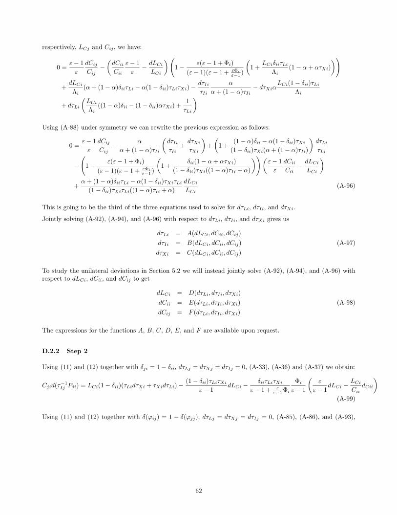
respectively, LCj and Cij , we have:

0 =ε− 1

ε

dCij

Cij−(dCii

Cii

ε− 1

ε− dLCi

LCi

)(1− ε(ε− 1 + Φi)

(ε− 1)(ε− 1 + εΦi

ε−1 )

(1 +

LCiδiiτLi

Λi(1− α+ ατXi)

))

+dLCi

Λi(α+ (1− α)δiiτLi − α(1− δii)τLiτXi)−

dτIiτIi

α

α+ (1− α)τIi− dτXiα

LCi(1− δii)τLi

Λi

+ dτLi

(LCi

Λi((1− α)δii − (1− δii)ατXi) +

1

τLi

)

Using (A-88) under symmetry we can rewrite the previous expression as follows:

0 =ε− 1

ε

dCij

Cij− α

α+ (1− α)τIi

(dτIiτIi

+dτXi

τXi

)+

(1 +

(1− α)δii − α(1− δii)τXi

(1− δii)τXi(α+ (1− α)τIi)

)dτLi

τLi

−(1− ε(ε− 1 + Φi)

(ε− 1)(ε− 1 + εΦi

ε−1 )

(1 +

δii(1− α+ ατXi)

(1− δii)τXi((1− α)τIi + α)

))(ε− 1

ε

dCii

Cii− dLCi

LCi

)

+α+ (1− α)δiiτLi − α(1− δii)τXiτLi

(1− δii)τXiτLi((1− α)τIi + α)

dLCi

LCi(A-96)

This is going to be the third of the three equations used to solve for dτLi, dτIi, and dτXi.

Jointly solving (A-92), (A-94), and (A-96) with respect to dτLi, dτIi, and dτXi gives us

dτLi = A(dLCi, dCii, dCij)

dτIi = B(dLCi, dCii, dCij) (A-97)

dτXi = C(dLCi, dCii, dCij)

To study the unilateral deviations in Section 5.2 we will instead jointly solve (A-92), (A-94), and (A-96) withrespect to dLCi, dCii, and dCij to get

dLCi = D(dτLi, dτIi, dτXi)

dCii = E(dτLi, dτIi, dτXi) (A-98)

dCij = F (dτLi, dτIi, dτXi)

The expressions for the functions A, B, C, D, E, and F are available upon request.

D.2.2 Step 2

Using (11) and (12) together with δji = 1− δii, dτLj = dτXj = dτIj = 0, (A-33), (A-36) and (A-37) we obtain:

Cjid(τ−1Ij Pji) = LCi(1− δii)(τLidτXi + τXidτLi)−

(1− δii)τLiτXi

ε− 1dLCi −

δiiτLiτXi

ε− 1 + εε−1Φi

Φi

ε− 1

(ε

ε− 1dLCi −

LCi

CiidCii

)

(A-99)

Using (11) and (12) together with δ(ϕij) = 1 − δ(ϕjj), dτLj = dτXj = dτIj = 0, (A-85), (A-86), and (A-93),

62

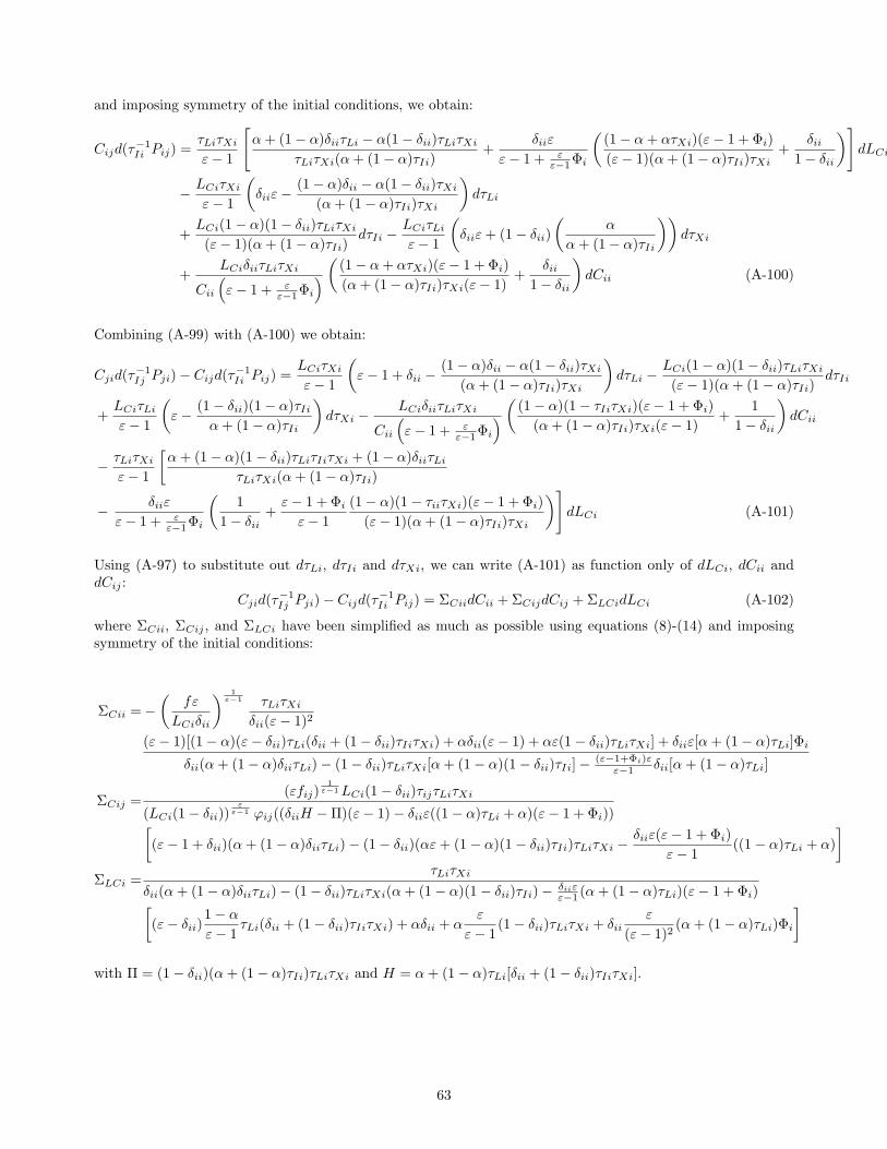
and imposing symmetry of the initial conditions, we obtain:

Cijd(τ−1Ii Pij) =

τLiτXi

ε− 1

[α+ (1− α)δiiτLi − α(1− δii)τLiτXi

τLiτXi(α+ (1− α)τIi)+

δiiε

ε− 1 + εε−1Φi

((1− α+ ατXi)(ε− 1 + Φi)

(ε− 1)(α+ (1− α)τIi)τXi+

δii1− δii

)]dLCi

− LCiτXi

ε− 1

(δiiε−



)dτLi

+LCi(1− α)(1− δii)τLiτXi

(ε− 1)(α+ (1− α)τIi)dτIi −

LCiτLi

ε− 1

(δiiε+ (1− δii)

(α

α+ (1− α)τIi

))dτXi

+LCiδiiτLiτXi

Cii

(ε− 1 + ε

ε−1Φi

)((1− α+ ατXi)(ε− 1 + Φi)

(α+ (1− α)τIi)τXi(ε− 1)+

δii1− δii

)dCii (A-100)

Combining (A-99) with (A-100) we obtain:


−1Ii Pij) =

LCiτXi

ε− 1

(ε− 1 + δii −



)dτLi −

LCi(1− α)(1− δii)τLiτXi

(ε− 1)(α+ (1− α)τIi)dτIi

+LCiτLi

ε− 1

(ε− (1− δii)(1− α)τIi

α+ (1− α)τIi

)dτXi −

LCiδiiτLiτXi

Cii

(ε− 1 + ε

ε−1Φi

)((1− α)(1− τIiτXi)(ε− 1 + Φi)

(α+ (1− α)τIi)τXi(ε− 1)+

1

1− δii

)dCii

− τLiτXi

ε− 1

[α+ (1− α)(1− δii)τLiτIiτXi + (1− α)δiiτLi

τLiτXi(α+ (1− α)τIi)

− δiiε

ε− 1 + εε−1Φi

(1

1− δii+

ε− 1 + Φi

ε− 1

(1− α)(1− τiiτXi)(ε− 1 + Φi)

(ε− 1)(α+ (1− α)τIi)τXi

)]dLCi (A-101)

Using (A-97) to substitute out dτLi, dτIi and dτXi, we can write (A-101) as function only of dLCi, dCii anddCij :


−1Ii Pij) = ΣCiidCii +ΣCijdCij +ΣLCidLCi (A-102)

where ΣCii, ΣCij , and ΣLCi have been simplified as much as possible using equations (8)-(14) and imposingsymmetry of the initial conditions:

ΣCii =−(

fε

LCiδii

) 1ε−1 τLiτXi

δii(ε− 1)2

(ε− 1)[(1− α)(ε− δii)τLi(δii + (1− δii)τIiτXi) + αδii(ε− 1) + αε(1− δii)τLiτXi] + δiiε[α+ (1− α)τLi]Φi

δii(α+ (1− α)δiiτLi)− (1− δii)τLiτXi[α+ (1− α)(1− δii)τIi]− (ε−1+Φi)εε−1 δii[α+ (1− α)τLi]

ΣCij =(εfij)

1ε−1LCi(1− δii)τijτLiτXi

(LCi(1− δii))ε

ε−1 ϕij((δiiH −Π)(ε− 1)− δiiε((1− α)τLi + α)(ε− 1 + Φi))[(ε− 1 + δii)(α+ (1− α)δiiτLi)− (1− δii)(αε+ (1− α)(1− δii)τIi)τLiτXi −


ε− 1((1− α)τLi + α)

]

ΣLCi =τLiτXi

δii(α+ (1− α)δiiτLi)− (1− δii)τLiτXi(α+ (1− α)(1− δii)τIi)− δiiεε−1 (α+ (1− α)τLi)(ε− 1 + Φi)[

(ε− δii)1− α

ε− 1τLi(δii + (1− δii)τIiτXi) + αδii + α

ε

ε− 1(1− δii)τLiτXi + δii

ε

(ε− 1)2(α+ (1− α)τLi)Φi

]

with Π = (1− δii)(α+ (1− α)τIi)τLiτXi and H = α+ (1− α)τLi[δii + (1− δii)τIiτXi].

63

D.2.3 Step 3

Using (12) and imposing symmetry of the initial conditions, one of the two consumption efficiency terms in (37)can be written as (τIi − 1)τ−1

Ii PijdCij = ECijdCij where:

ECij = (τIi − 1)

(εfij

LCi(1− δii)

) 1ε−1 ετijτLiτXi

(ε− 1)ϕij

Therefore,

ΩCij ≡ ΣCij + ECij =ΩCijτijτLiτXi(εfij)

1ε−1

ϕij(ε− 1)(LCi(1− δii))1

ε−1 [(δiiH −Π)(ε− 1)− δiiε((1− α)τLi + α)(ε− 1 + Φi)]

where

ΩCij = (ε− 1)((ε− 1)(1− δii)H + ετIi(δiiH −Π))− δiiε(ε− 1 + Φi)((1− α)τLi + α)(ετIi − ε+ 1) (A-103)

Using (12), the second consumption efficiency term in (37) can be written as (τXi−1)PiidCii = ECiidCii where:

ECii = (τXi − 1)

(εfii

LCiδii

) 1ε−1 ετLi

(ε− 1)ϕii

Therefore,

ΩCii ≡ ΣCii + ECii =

(εfii

LCiδii

) 1ε−1 τLi

ϕii(ε− 1)2

ΩCii

δii(α+ (1− α)δiiτLi)− (1− δii)τLiτXi(α+ (1− α)(1− δii)τIi)− (ε−1+Φi)εε−1 (α+ (1− α)τLi)

where

ΩCii ≡(1− τXi)[ε(ε− 1)(δii(α+ (1− α)δiiτLi)− (1− δii)τLiτXi(α+ (1− α)(1− δii)τIi))

− (ε− 1 + Φi)ε2δii(α+ (1− α)τLi)]

− τXi[(ε− 1)(ε(1− α)τLi(δii + (1− δii)τIiτXi)− (1− α)δiiτLi(δii + (1− δii)τIiτXi)

+ αδii(ε− 1) + αε(1− δii)τLiτXi) + δiiε(α+ (1− α)τLi)Φi] (A-104)

The production efficiency term in (37) is given by(

εε−1τLiτXi − 1

)dLCi. Let us define ELCi ≡ ε

ε−1τLiτXi − 1.

Then,

ΩLCi ≡ ΣLCi + ELCi =

=ΩLCi(ε− 1)−1

δii(α+ (1− α)δiiτLi)− (1− δii)τLiτXi(α+ (1− α)(1− δii)τIi)− δiiεε−1 (α+ (1− α)τLi)(ε− 1 + Φi)

where

ΩLCi ≡ δii(ε− 1)τLiτXi[α+ (1− α)τLi(δii + (1− δii)τIiτXi)− ε(α+ (1− α)τLi)]

− (ε− 1)[δii(α+ (1− α)δiiτLi)− (1− δii)τLiτXi(α+ (1− α)(1− δii)τIi)− δiiε(α+ (1− α)τLi)]

− (τLiτXi − 1)δiiε(α+ (1− α)τLi)Φi (A-105)

64

D.3 Preliminary steps to study unilateral policy changes in the one-sector model

In the special case α = 1, i.e., when there is no homogeneous sector, we can apply some simplifications to the totaldifferentials defined in A.8. Indeed in this case Zi = 0 and LCi = L for i = H,F so that dZi = dLCi = dτLi = 0for i = H,F . Also, Wj = 1 so that dWj = 0 for j = F . Finally, we set τLi = 1 for i = H,F since the free-tradeallocation is efficient in this case. After taking the differentials we also impose symmetry of the initial free-tradeallocation (τIi = τXi = 1 for i = H,F ) as well as dτIj = dτXj = 0 for j = F .

First, consider the case of heterogeneous firms. Our objective is to retrieve 4 conditions as a function ofdWi, dCii, dCij , dτIi and dτXi. We proceed in 4 steps.

(1) First, recall that (A-38) simplifies to:

dϕij =ϕij

ϕiidϕii −

ε

ε− 1ϕijdWi +

ε

ε− 1ϕijdτTij , i, j = H,F, i 6= j (A-106)

Second, from (A-36) we have:

dϕii = − ϕii

Cii

(ε− 1 + ε

ε−1Φi

)dCii, i = H,F (A-107)

Third, from (A-106) we have dϕjj =ϕjj

ϕjidϕji − ε

ε−1ϕjjdτTji which, using (A-33), (A-107), and dτTji = dτXi

when i = H, j = F , can be written as:

dϕjj =ϕjj

Cii

(ε− 1 + ε

ε−1Φi

) δii1− δii

dCii −ε

ε− 1ϕjjdτXi, i = H, j = F (A-108)

Finally, using (A-33) to express dϕij together with (A-108) to substitute out dϕjj we have:

dϕij =δjj

1− δjjϕij

1

Cii

(ε− 1 + ε

ε−1Φi

) δii1− δii

dCii +ε

ε− 1dτXi

, i = H, j = F (A-109)

Using (A-107), (A-109), δjj = δii, and dτTij = dτIi when i = H, j = F , we can rewrite (A-106) as follows:

(1− δii)dWi − (1− δii)dτIi + δiidτXi +1− 2δii

(1− δii)(ε− 1 + ε

ε−1Φi

) ε− 1

ε

dCii

Cii= 0, i = H, j = F (A-110)

(2) Recall that (13) simplifies to (A-26) which, using (11) and (12) together with LCi = L for i = H,F ,δji = 1− δii for i, j = H,F , τIj = τXj = 1 for j = F , and τLi = 1 for i = H,F , can be rewritten as:

L(1− δii)τXiWi − L(1− δjj) = 0, i = H, j = F (A-111)

Using (A-34) for i = j together with (A-108) we can write:

dδjj = δii(ε− 1 + Φi)

ε

ε− 1dτXi −

δii1− δii

1(ε− 1 + ε

ε−1Φi

) dCii

Cii

(A-112)

Taking the total differential of (A-111) and using (A-112) to substitute out dδjj , and (A-34) to substitute outdδii, we have:

dWi +

(1 +


(ε− 1)(1− δii)

)dτXi −

δii(ε− 1 + Φi)

Cii(1− δii)2(ε− 1 + εε−1Φi)

dCii = 0, i = H, j = F (A-113)

65

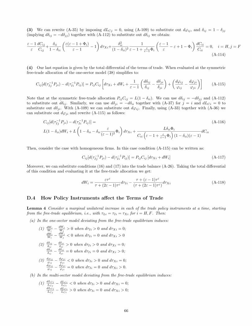
(3) We can rewrite (A-35) by imposing dLCj = 0, using (A-109) to substitute out dϕij , and δij = 1 − δjj(implying dδij = −dδjj) together with (A-112) to substitute out dδij we obtain:

ε− 1

ε

dCij

Cij+

δii1− δii

(ε(ε− 1 + Φi)

ε− 1− 1

)dτXi+

δ2ii(1− δii)2

1

ε− 1 + εε−1Φi

(ε− 1

ε− ε+ 1− Φi

)dCii

Cii= 0, i = H, j = F

(A-114)

(4) Our last equation is given by the total differential of the terms of trade. When evaluated at the symmetricfree-trade allocation of the one-sector model (38) simplifies to:


Ii Pij)] = PijCij

[dτXi + dWi +

1

ε− 1

(dδijδij

− dδjiδji

)+

(dϕij

ϕij− dϕji

ϕji

)](A-115)

Note that at the symmetric free-trade allocation PijCij = L(1 − δii). We can use dδij = −dδjj and (A-112)to substitute out dδij . Similarly, we can use dδji = −dδii together with (A-37) for j = i and dLCi = 0 tosubstitute out dδji. With (A-109) we can substitute out dϕij . Finally, using (A-33) together with (A-36) wecan substitute out dϕji and rewrite (A-115) as follows:


Ii Pij)] = (A-116)

L(1− δii)dWi + L

(1− δii − δii

ε

(ε− 1)2Φi

)dτXi +

LδiiΦi

Cii

(ε− 1 + ε

ε−1Φi

)(1− δii)(ε− 1)

dCii

Then, consider the case with homogeneous firms. In this case condition (A-115) can be written as:


Ii Pij)] = PijCij [dτXi + dWi] (A-117)

Moreover, we can substitute conditions (16) and (17) into the trade balance (A-26). Taking the total differentialof this condition and evaluating it at the free-trade allocation we get:

dWi =ετ ε

τ + (2ε− 1)τ εdτIi −

τ + (ε− 1)τ ε

(τ + (2ε− 1)τ ε)dτXi (A-118)

D.4 How Policy Instruments affect the Terms of Trade

Lemma 4 Consider a marginal unilateral increase in each of the trade policy instruments at a time, startingfrom the free-trade equilibrium, i.e., with τLi = τIi = τXi for i = H,F . Then:

(a) In the one-sector model deviating from the free-trade equilibrium induces:

(1) dWi

Wi− dWj

Wj> 0 when dτIi > 0 and dτXi = 0;

dWi

Wi− dWj

Wj< 0 when dτIi = 0 and dτXi > 0

(2)dδijδij

− dδjiδji

> 0 when dτIi > 0 and dτXi = 0;dδijδij

− dδjiδji

= 0 when dτIi = 0 and dτXi > 0;

(3)dϕij

ϕij− dϕji

ϕji< 0 when dτIi > 0 and dτXi = 0;

dϕij

ϕij− dϕji

ϕji= 0 when dτIi = 0 and dτXi > 0.

(b) In the multi-sector model deviating from the free-trade equilibrium induces:

(1)dLCj

LCj− dLCi

LCi< 0 when dτIi > 0 and dτXi = 0;

dLCj

LCj− dLCi

LCi> 0 when dτIi = 0 and dτXi > 0;

66

(2)dδijδij

− dδjiδji

< 0 ⇐⇒ δii > 1/2 when dτIi > 0 and dτXi = 0;dδijδij

− dδjiδji

> 0 ⇐⇒ δii > 1/2 when dτIi = 0 and dτXi > 0;

(3)dϕij

ϕij− dϕji

ϕji> 0 ⇐⇒ δii > 1/2 when dτIi > 0 and dτXi = 0;

dϕij

ϕij− dϕji

ϕji< 0 ⇐⇒ δii > 1/2 when dτIi = 0 and dτXi > 0.

Proof

(a) (1) Combining conditions (A-114), (A-113) and (A-110) we find dCii, dWi and dCij ad a function of thedeviations of the policy instruments. In particular it can be shown that at free trade:

dWi = awdτIi + bwdτXi

where aw = δiidτIiε(Φi+ε−1)δiiΦiε+(ε−1)(1−δii+δii(ε−1)) > 0 since ε > 1 and 0 < δii < 1. Moreover bw = −1.

(2) Recall that dδji = −dδii for i, j = H,F and j 6= i . Then we can use (A-112) and its symmetriccounterpart to obtain:

dδijδij

− dδjiδji

= aδdτIi

where aδ = − δiiεφij(ε−1+Φi)δiiΦiε+(ε−1)(1−δii+δii(ε−1)) < 0 for ε > 1 and 0 < δii < 1.

(3) Using the solution for dCii found in point (a), condition (A-109) and their symmetric counterpartswe obtain:

dϕij

ϕij− dϕji

ϕji= aϕdτIi

where aϕ = − δiiεφij

δiiΦiε+(ε−1)(1−δii+δii(ε−1)) < 0 for ε > 1 and 0 < δii < 1.

(b) (1) Using (A-93) together with (A-98), imposing symmetry of the initial conditions and τLi = τIi =τXi = 1, and setting to zero dτLi, dτLj , dτIj and dτXj we obtain:

dLCj

LCj− dLCi

LCi= a1dτIi + a2dτXi

where a1 ≡ − (1−δii)[(ε−1)(1−α+2δii(ε−1+α))+2δiiεΦi](1−2δii)2(ε−1) < 0 and a2 ≡ (1−δii)[(1+α+2δii(ε−1−α))(ε−1)+2δiiεΦi]

(1−2δii)2(ε−1) >

0. To see that a2 > 0 it is enough to notice that a3(δii) ≡ 1 + α+ 2δii(ε− 1− α) is linear in δii andthat a3(0) = 1 + α > 0 and a3(1) = 2ε− 1− α > 0.

(2) Recall that δji = 1− δii, implying that dδji = −dδii and dδij = −dδjj . Using (A-37) to compute dδiiand (A-86) to compute dδjj , together with (A-98), imposing symmetry of the initial conditions andτLi = τIi = τXi = 1, and setting to zero dτLi, dτLj , dτIj and dτXj we obtain:

dδijδij

− dδjiδji

= b1 (dτIi − dτXi)

where b1 ≡ − (1−δii)δiiε(ε−1+Φi)δij(ε−1)(2δii−1) < 0 ⇐⇒ δii > 1/2;

(3) Using (A-33) and (A-36) to compute dϕji and (A-85) to compute dϕij , together with (A-98), imposingsymmetry of the initial conditions and τLi = τIi = τXi = 1, and setting to zero dτLi, dτLj , dτIj anddτXj , we obtain:

dϕij

ϕij− dϕji

ϕji= c1 (dτIi − dτXi)

where c1 ≡ δiiε(2δii−1)(ε−1) > 0 ⇐⇒ δii > 1/2.

67

D.5 Proof of Lemma 1

We prove Lemma 1 point by point.

(a) From Proposition 4 (b) (iii) we know that the free-trade allocation is Pareto optimal in the one-sectormodel, implying that the production-efficiency wedge is zero for all policy instruments. Formally, in the one-sector model dLCi = 0 in (37).

(b) When τIi = τXi = 1, the consumption-efficiency wedge in (37) is zero for any dCii and dCij .

(c) In the case of heterogeneous firms, we can use (A-116) to write the terms-of-trade effect in (37) as functionof dWi, dCii, and dτXi. The equations (A-110), (A-113), and (A-114) give us a linear system of equations thatwe can solve to express:

dCii = A(dτIi, dτXi)

dWi = B(dτIi, dτXi) (A-119)

dCij = C(dτIi, dτXi)

The expressions for A, B, and C are available upon request. Using (A-119) we can substitute out dWi and dCii

from (A-116), and express the terms-of-trade effect as function only of dτIi and dτXi:


Ii Pij)] = a dτIi + b dτXi

where

a =L(1− δii)δiiε((ε− 1)2 + εΦi)

(ε− 1)[(ε− 1)(1− δii + δii(ε− 1)) + εδiiΦi]> 0

b = 0

This means that a small positive import tax generates a positive terms-of-trade effect while small changes inτXi do not produce terms-of-trade effects.

In the case of homogeneous firms, if we substitute (A-118) into (A-117) we get:


Ii Pij)] = c dτIi + d dτXi

where

c =ετ ε

τ + (2ε− 1)τ ε> 0

d =ετ ε

τ + (2ε− 1)τ ε> 0

This means that the net terms-of-trade effect of a small tariff or a small export tax is positive.

(d) Follows from the previous points.

68

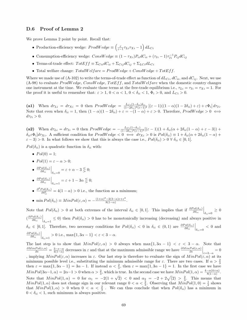
D.6 Proof of Lemma 2

We prove Lemma 2 point by point. Recall that:

• Production-efficiency wedge: ProdWedge ≡(

εε−1τLiτXi − 1

)dLCi

• Consumption-efficiency wedge: ConsWedge ≡ (1− τXi)PiidCii + (τIi − 1)τ−1Ii PijdCij

• Terms-of-trade effect: TotEff ≡ ΣCiidCii +ΣCijdCij +ΣLCidLCi

• Total welfare change: TotalWelfare = ProdWedge+ ConsWedge+ TotEff .

Where we made use of (A-102) to write the terms-of-trade effect as function of dLCi, dCii, and dCij . Next, we use(A-98) to evaluate ProdWedge, ConsWedge, TotEff , and TotalWelfare when the domestic country changesone instrument at the time. We evaluate those terms at the free-trade equilibrium i.e., τLi = τIi = τXi = 1. Forthe proof it is useful to remember that: ε > 1, 0 < α < 1, 0 < δii < 1, Φi > 0, and LCi > 0.

(a1) When dτLi = dτXi = 0 then ProdWedge = LCi(1−δii)δii(1−2δii)2(ε−1)2 [(ε− 1)((1− α)(1− 2δii) + ε) + εΦi] dτIi.

Note that even when δii = 1, then (1− α)(1− 2δii) + ε = −(1− α) + ε > 0. Therefore, ProdWedge > 0 ⇐⇒dτIi > 0.

(a2) When dτLi = dτIi = 0 then ProdWedge = − LCi(1−δii)(1−2δii)2(ε−1)2 [(ε − 1)(1 + δii(α + 2δii(1 − α) + ε − 3)) +

δiiεΦi]dτXi. A sufficient condition for ProdWedge < 0 ⇐⇒ dτXi > 0 is Pol(δii) ≡ 1 + δii(α + 2δii(1 − α) +ε− 3) > 0. In what follows we show that this is always the case i.e., Pol(δii) > 0 ∀ δii ∈ [0, 1].

Pol(δii) is a quadratic function in δii with:

• Pol(0) = 1;

• Pol(1) = ε− α > 0;

• ∂Pol(δii)∂δii

∣∣∣δii=0

= ε+ α− 3 ⋚ 0;


∣∣∣δii=1

= ε+ 1− 3α ⋚ 0;

• ∂2Pol(δii)∂δ2ii

= 4(1− α) > 0 i.e., the function as a minimum;

• minPol(δii) ≡ MinPol(ε, α) = − (1+α)2−2(3−α)ε+ε2

8(1−α) .

Note that Pol(δii) > 0 at both extremes of the interval δii ∈ [0, 1]. This implies that if ∂Pol(δii)∂δii

∣∣∣δii=0

≥ 0

(∂Pol(δii)∂δii

∣∣∣δii=1

≤ 0) then Pol(δii) > 0 has to be monotonically increasing (decreasing) and always positive in

δii ∈ [0, 1]. Therefore, two necessary conditions for Pol(δii) < 0 in δii ∈ (0, 1) are ∂Pol(δii)∂δii

∣∣∣δii=0

< 0 and

∂Pol(δii)∂δii

∣∣∣δii=1

> 0 i.e., max1, 3α− 1 < ε < 3− α.

The last step is to show that MinPol(ε, α) > 0 always when max1, 3α − 1 < ε < 3 − α. Note that∂MinPol(ε,α)

∂ε = 3−ε−α4(1−α) decreases in ε and that at the maximum admissible range we have ∂MinPol(ε,α)

∂ε

∣∣∣ε=3−α

= 0

, implying MinPol(ε, α) increases in ε. Our last step is therefore to evaluate the sign of MinPol(ε, α) at itsminimum possible level i.e., substituting the minimum admissible range for ε. There are two cases. If α > 2

3then ε = max1, 3α − 1 = 3α − 1. If instead α < 2

3 , then ε = max1, 3α − 1 = 1. In the first case we have

MinPol(3α−1, α) = 2α−1 > 0 when α > 23 , which is true. In the second case we haveMinPol(1, α) = 4−α(4+α)

8(1−α) .

Note that MinPol(1, α) = 0 for α1 = −2(1 +√2) < 0 and α2 = −2 + 2

√(2) > 2

3 . This means thatMinPol(1, α) does not change sign in our relevant range 0 < α < 2

3 . Observing that MinPol(1, 0) = 12 shows

that MinPol(1, α) > 0 when 0 < α < 23 . We can thus conclude that when Pol(δii) has a minimum in

0 < δii < 1, such minimum is always positive.

69

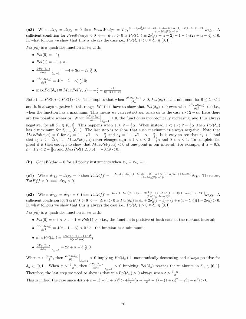
(a3) When dτIi = dτXi = 0 then ProdWedge = LCi(ε−1)[2δ2ii(ε+α−2)−1−δii(2ε+α−4)]−2(1−δii)δiiεΦi

(1−2δii)2(ε−1)2 dτLi. A

sufficient condition for ProdWedge < 0 ⇐⇒ dτLi > 0 is Pol(δii) ≡ 2δ2ii(ε + α − 2) − 1 − δii(2ε + α − 4) < 0.In what follows we show that this is always the case i.e., Pol(δii) < 0 ∀ δii ∈ [0, 1].


• Pol(0) = −1;

• Pol(1) = −1 + α;


∣∣∣δii=1

= −4 + 3α+ 2ε ⋚ 0;


= 4(ε− 2 + α) ⋚ 0;

• maxPol(δii) ≡ MaxPol(ε, α) = − ε2 − α2

8(−2+α+ε) .

Note that Pol(0) < Pol(1) < 0. This implies that when ∂2Pol(δii)∂δ2ii

> 0, Pol(δii) has a minimum for 0 ≤ δii < 1

and it is always negative in this range. We thus have to show that Pol(δii) < 0 even when ∂2Pol(δii)∂δ2ii

< 0 i.e.,

when the function has a maximum. This means we can restrict our analysis to the case ε < 2− α. Here there

are two possible scenarios. When ∂Pol(δii)∂δii

∣∣∣δii=1

≥ 0, the function is monotonically increasing, and thus always

negative, for all δii ∈ (0, 1]. This happens when ε ≥ 2 − 32α. When instead 1 < ε < 2 − 3

2α, then Pol(δii)has a maximum for δii ∈ (0, 1). The last step is to show that such maximum is always negative. Note thatMaxPol(ε, α) = 0 for ε1 = 1 −

√1− α − α

2 and ε2 = 1 +√1− α − α

2 . It is easy to see that ε1 < 1 andthat ε2 > 2 − 3

2α, i.e., MaxPol(ε, α) never changes sign in 1 < ε < 2 − 32α and 0 < α < 1. To complete the

proof it is then enough to show that MaxPol(ε, α) < 0 at one point in our interval. For example, if α = 0.5,ε = 1.2 < 2− 3

2α and MaxPol(1.2, 0.5) = −0.49 < 0.

(b) ConsWedge = 0 for all policy instruments when τIi = τXi = 1.

(c1) When dτLi = dτXi = 0 then TotEff = −LCi(1−δii)[(1−δii)(ε−1)(1−α+(ε−1+α)2δii)+δiiεΦi](1−2δii)2(ε−1)2 dτIi. Therefore,

TotEff < 0 ⇐⇒ dτIi > 0.

(c2) When dτLi = dτIi = 0 then TotEff =LCi(1−δii)[(ε−1)(δii+2δ2ii(ε−1)+(ε+α(1−δii))(1−2δii))+δiiεΦi]

(1−2δii)2(ε−1)2 dτXi. A

sufficient condition for TotEff > 0 ⇐⇒ dτXi > 0 is Pol(δii) ≡ δii +2δ2ii(ε− 1)+ (ε+α(1− δii))(1− 2δii) > 0.In what follows we show that this is always the case i.e., Pol(δii) > 0 ∀ δii ∈ [0, 1].


• Pol(0) = ε+ α > ε− 1 = Pol(1) > 0 i.e., the function is positive at both ends of the relevant interval;


= 4(ε− 1 + α) > 0 i.e., the function as a minimum;

• minPol(δii) =4ε(α+ε−1)−(1+α)2

8(ε−1+α) ;


∣∣∣δii=1

= 2ε+ α− 3 ⋚ 0.

When ε < 3−α2 , then ∂Pol(δii)

∂δii

∣∣∣δii=1

< 0 implying Pol(δii) is monotonically decreasing and always positive for

δii ∈ [0, 1]. When ε > 3−α2 , then ∂Pol(δii)

∂δii

∣∣∣δii=1

> 0 implying Pol(δii) reaches the minimum in δii ∈ [0, 1].

Therefore, the last step we need to show is that minPol(δii) > 0 always when ε > 3−α2 .

This is indeed the case since 4ε(α+ ε− 1)− (1 + α)2 > 4 3−α2 (α+ 3−α

2 − 1)− (1 + α)2 = 2(1− α2) > 0.

70

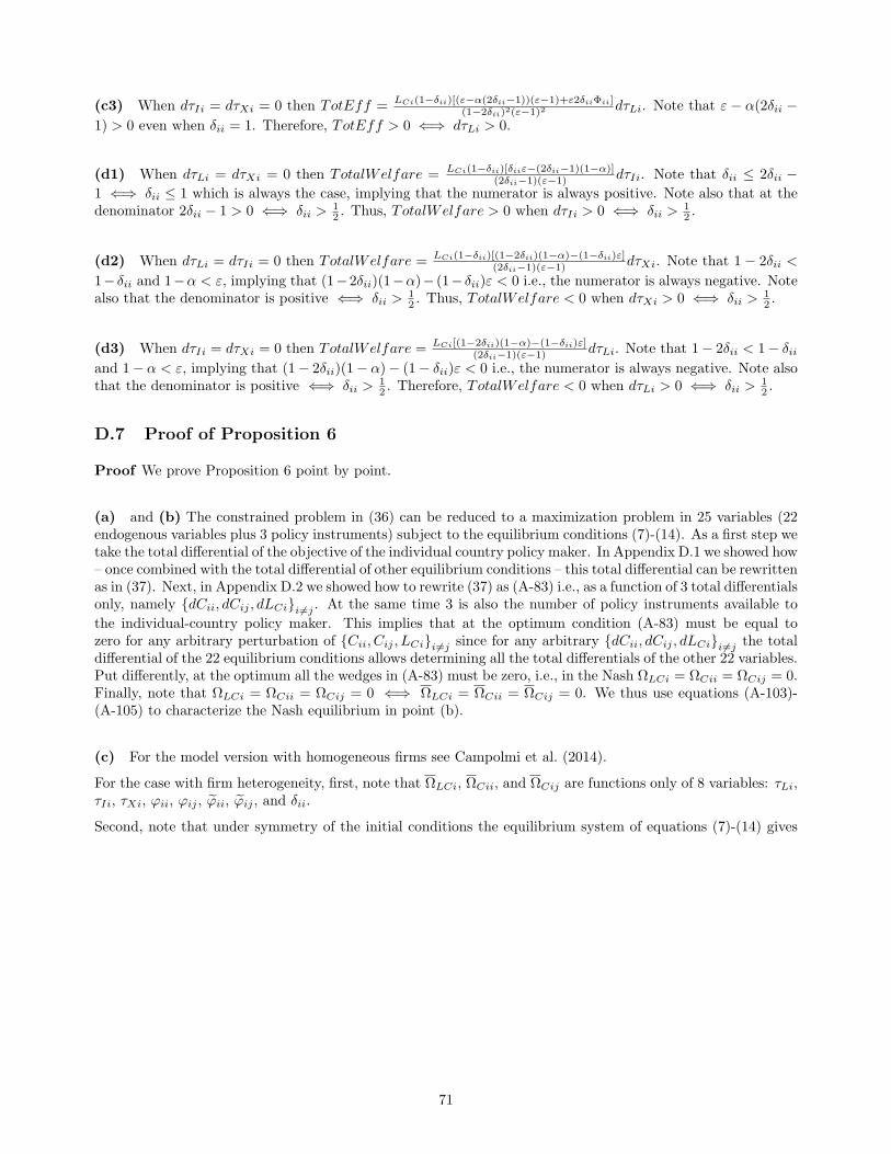
(c3) When dτIi = dτXi = 0 then TotEff = LCi(1−δii)[(ε−α(2δii−1))(ε−1)+ε2δiiΦii](1−2δii)2(ε−1)2 dτLi. Note that ε − α(2δii −

1) > 0 even when δii = 1. Therefore, TotEff > 0 ⇐⇒ dτLi > 0.

(d1) When dτLi = dτXi = 0 then TotalWelfare = LCi(1−δii)[δiiε−(2δii−1)(1−α)](2δii−1)(ε−1) dτIi. Note that δii ≤ 2δii −

1 ⇐⇒ δii ≤ 1 which is always the case, implying that the numerator is always positive. Note also that at thedenominator 2δii − 1 > 0 ⇐⇒ δii >

12 . Thus, TotalWelfare > 0 when dτIi > 0 ⇐⇒ δii >

12 .

(d2) When dτLi = dτIi = 0 then TotalWelfare = LCi(1−δii)[(1−2δii)(1−α)−(1−δii)ε](2δii−1)(ε−1) dτXi. Note that 1− 2δii <

1− δii and 1−α < ε, implying that (1−2δii)(1−α)− (1− δii)ε < 0 i.e., the numerator is always negative. Notealso that the denominator is positive ⇐⇒ δii >

12 . Thus, TotalWelfare < 0 when dτXi > 0 ⇐⇒ δii >

12 .

(d3) When dτIi = dτXi = 0 then TotalWelfare = LCi[(1−2δii)(1−α)−(1−δii)ε](2δii−1)(ε−1) dτLi. Note that 1− 2δii < 1− δii

and 1− α < ε, implying that (1− 2δii)(1− α)− (1− δii)ε < 0 i.e., the numerator is always negative. Note alsothat the denominator is positive ⇐⇒ δii >

12 . Therefore, TotalWelfare < 0 when dτLi > 0 ⇐⇒ δii >

12 .



(a) and (b) The constrained problem in (36) can be reduced to a maximization problem in 25 variables (22endogenous variables plus 3 policy instruments) subject to the equilibrium conditions (7)-(14). As a first step wetake the total differential of the objective of the individual country policy maker. In Appendix D.1 we showed how– once combined with the total differential of other equilibrium conditions – this total differential can be rewrittenas in (37). Next, in Appendix D.2 we showed how to rewrite (37) as (A-83) i.e., as a function of 3 total differentialsonly, namely dCii, dCij , dLCii 6=j . At the same time 3 is also the number of policy instruments available to

the individual-country policy maker. This implies that at the optimum condition (A-83) must be equal tozero for any arbitrary perturbation of Cii, Cij , LCii 6=j since for any arbitrary dCii, dCij , dLCii 6=j the totaldifferential of the 22 equilibrium conditions allows determining all the total differentials of the other 22 variables.Put differently, at the optimum all the wedges in (A-83) must be zero, i.e., in the Nash ΩLCi = ΩCii = ΩCij = 0.Finally, note that ΩLCi = ΩCii = ΩCij = 0 ⇐⇒ ΩLCi = ΩCii = ΩCij = 0. We thus use equations (A-103)-(A-105) to characterize the Nash equilibrium in point (b).

(c) For the model version with homogeneous firms see Campolmi et al. (2014).

For the case with firm heterogeneity, first, note that ΩLCi, ΩCii, and ΩCij are functions only of 8 variables: τLi,τIi, τXi, ϕii, ϕij , ϕii, ϕij , and δii.

Second, note that under symmetry of the initial conditions the equilibrium system of equations (7)-(14) gives

71

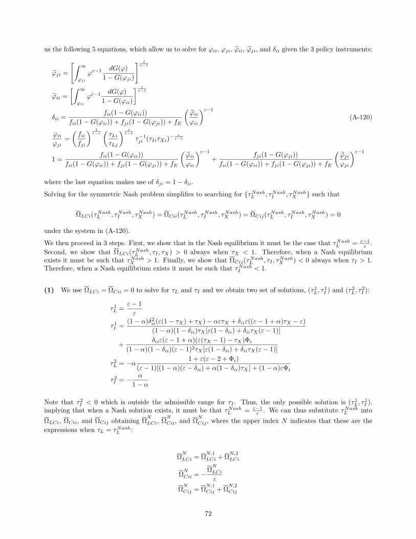
us the following 5 equations, which allow us to solve for ϕii, ϕji, ϕii, ϕji, and δii given the 3 policy instruments:

ϕji =

[∫ ∞

ϕji

ϕε−1 dG(ϕ)

1−G(ϕji)

] 1ε−1

ϕii =

[∫ ∞

ϕii

ϕε−1 dG(ϕ)

1−G(ϕii)

] 1ε−1

δii =fii(1−G(ϕii))

fii(1−G(ϕii)) + fji(1−G(ϕji)) + fE

(ϕii

ϕii

)ε−1

(A-120)

ϕii

ϕji=

(fiifji

) 1ε−1(τLi

τLj

) εε−1

τ−1ji (τIiτXi)

− εε−1

1 =fii(1−G(ϕii))


(ϕii

ϕii

)ε−1

+fji(1−G(ϕji))


(ϕji

ϕji

)ε−1

where the last equation makes use of δji = 1− δii.

Solving for the symmetric Nash problem simplifies to searching for τNashL , τNash

I , τNashX such that

ΩLCi(τNashL , τNash

I , τNashX ) = ΩCii(τ

NashL , τNash

I , τNashX ) = ΩCij(τ

NashL , τNash

I , τNashX ) = 0

under the system in (A-120).

We then proceed in 3 steps. First, we show that in the Nash equilibrium it must be the case that τNashL = ε−1

ε .

Second, we show that ΩLCi(τNashL , τI , τX) > 0 always when τX < 1. Therefore, when a Nash equilibrium

exists it must be such that τNashX > 1. Finally, we show that ΩCij(τ

NashL , τI , τ

NashX ) < 0 always when τI > 1.

Therefore, when a Nash equilibrium exists it must be such that τNashI < 1.

(1) We use ΩLCi = ΩCii = 0 to solve for τL and τI and we obtain two set of solutions, (τ1L, τ1I ) and (τ2L, τ

2I ):

τ1L =ε− 1

ε

τ1I =(1− α)δ2ii(ε(1− τX) + τX)− αετX + δiiε((ε− 1 + α)τX − ε)

(1− α)(1− δii)τX [ε(1− δii) + δiiτX(ε− 1)]

+δiiε(ε− 1 + α)(ε(τX − 1)− τX)Φi

(1− α)(1− δii)(ε− 1)2τX [ε(1− δii) + δiiτX(ε− 1)]

τ2L = −α1 + ε(ε− 2 + Φi)

(ε− 1)[(1− α)(ε− δii) + α(1− δii)τX ] + (1− α)εΦi

τ2I = − α

1− α

Note that τ2I < 0 which is outside the admissible range for τI . Thus, the only possible solution is (τ1L, τ1I ),

implying that when a Nash solution exists, it must be that τNashL = ε−1

ε . We can thus substitute τNashL into

ΩLCi, ΩCii, and ΩCij obtaining ΩN

LCi, ΩN

Cii, and ΩN

Cij , where the upper index N indicates that these are the

expressions when τL = τNashL :

ΩN

LCi = ΩN,1

LCi +ΩN,2

LCi

ΩN

Cii = −ΩN

LCi

ε

ΩN

Cij = ΩN,1

Cij +ΩN,2

Cij

72

where

ΩN,1

LCi ≡ (ε− 1)2[δii(ε− (ε− 1)τX)(ε− (1− α)δii) + δii(ε− 1)τX((1− α)(1− δii)τIτX)

+ ε((1− δii)(α+ (1− α)(1− δii)τI)τX)]

ΩN,2

LCi ≡ δiiε(ε− 1 + α)(ε− (ε− 1)τX)Φi

ΩN,1

Cij ≡ (ε− 1)

[δii(ε− 1 + α)(ε(1− τI)− 1) + δiiτI(αε+ δii(ε− 1)(1− α)) + (1− δii)(ε− 1)

(α+

δii(1− α)(ε− 1)

ε

)

+(1− δii)(ε− 1)τIτX

((1− α)(ε− 1)(1− δii)

ε− α− (1− α)(1− δii)τI

)]

ΩN,2

Cij ≡ δii(ε− 1 + α)(ε(1− τI)− 1)Φi

Note that ΩN

Cii and ΩN

LCi are collinear. In the next steps we can thus concentrate on ΩN

LCi and ΩN

Cij to

characterize the Nash solution for the remaining two instruments, τNashX and τNash

I .

(2) First, note that ε − (ε − 1)τX > 0 ⇐⇒ τX < εε−1 . This implies that when τX < ε

ε−1 we have both

ΩN,1

LCi > 0 and ΩN,2

LCi > 0, Therefore, ΩN

LCi > 0∀τX < εε−1 , implying that there cannot be a Nash equilibrium in

this region as it will never be the case that ΩN

LCi = 0. Thus, in the Nash it must the case that τNashX > ε

ε−1 > 1.

(3) The last thing we need to show is that τNashI < 1. We prove this by contradiction.

Assume τNashI > 1. In the previous point we already showed that τNash

X > 1, thus we also have τNashI τNash

X > 1.

First, note that ΩN,2

Cij < 0 when τNashI > 1. Thus, a necessary condition for the Nash equilibrium to exist in the

region τI > 1 is that ∃τI > 1 such that ΩN,1

Cij > 0.

Next, note that ΩN,1

Cij is function of the two tax instruments, the endogenous variable δii, and the parametersα and ε. Note also that δii is an implicit function of the tax instruments, the fix costs f and fx, ε, and thedistribution function for firms’ productivities G(ϕ), but not of α, as can be seen from the system (A-120). Thus,

ΩN,1

Cij is linear in α. Note that:

ΩN,1

Cij

∣∣∣∣α=0

= (ε− 1)2[−δii(1− δii + ε(τI − 1)(ε− δii))− (1− δii)

2(1 + ε(τI − 1))τIτX]< 0

ΩN,1

Cij

∣∣∣∣α=1

= −(ε− 1)2[(τIτX − 1)(1− δii) + δiiε(τI − 1)] < 0

This implies that ΩN,1

Cij < 0 for all τI > 1. Therefore, ΩN

Cij < 0 for all τI > 1 which contradict our original

hypothesis of a Nash equilibrium with τNashI > 1. Thus, if a Nash equilibrium exists it must be such that

τNashI < 1.


Proof

(a) When only labor taxes are available τIi = τXi = 1 and dτIi = dτXi = 0 for i = H,F . Therefore, (37)

73

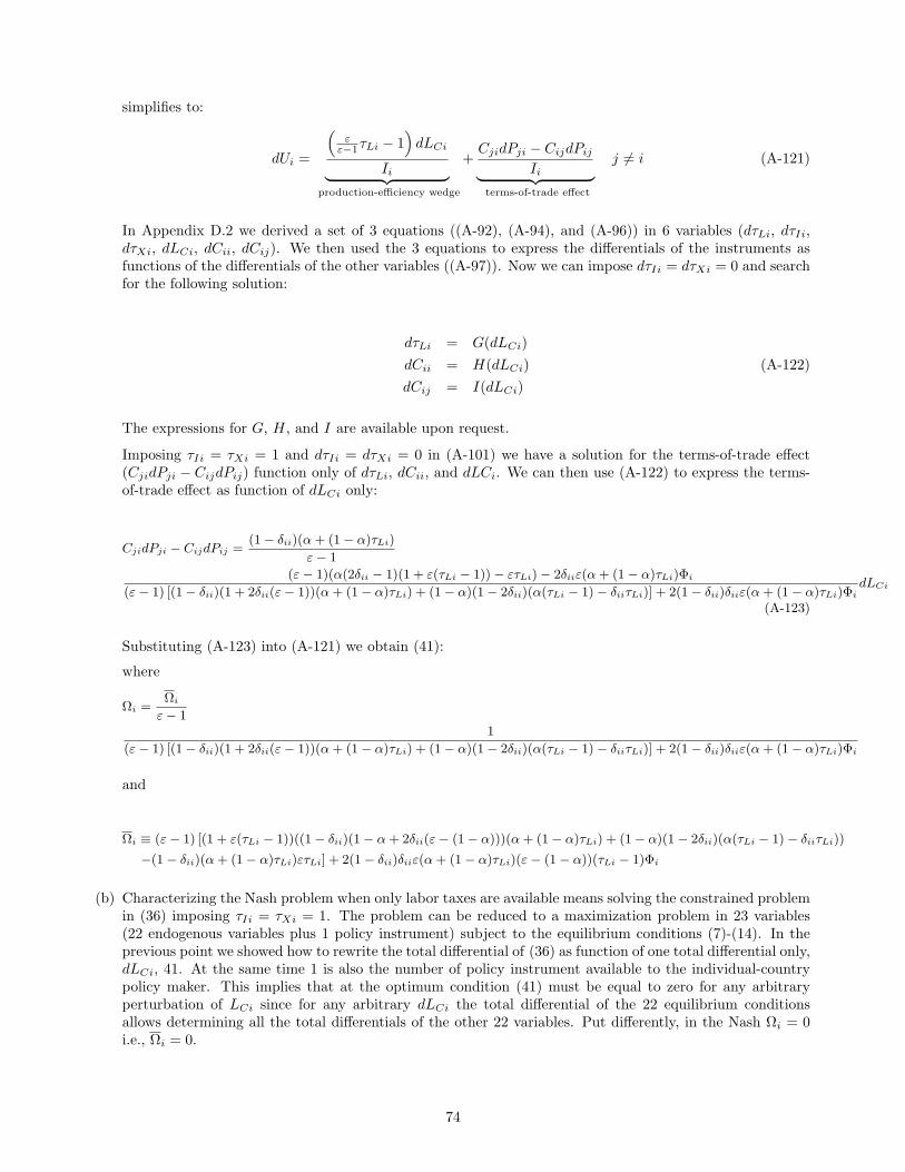
simplifies to:

dUi =

(ε

ε−1τLi − 1)dLCi

Ii︸︷︷︸production-efficiency wedge

+CjidPji − CijdPij

Ii︸︷︷︸terms-of-trade effect

j 6= i (A-121)

In Appendix D.2 we derived a set of 3 equations ((A-92), (A-94), and (A-96)) in 6 variables (dτLi, dτIi,dτXi, dLCi, dCii, dCij). We then used the 3 equations to express the differentials of the instruments asfunctions of the differentials of the other variables ((A-97)). Now we can impose dτIi = dτXi = 0 and searchfor the following solution:

dτLi = G(dLCi)

dCii = H(dLCi) (A-122)

dCij = I(dLCi)

The expressions for G, H, and I are available upon request.

Imposing τIi = τXi = 1 and dτIi = dτXi = 0 in (A-101) we have a solution for the terms-of-trade effect(CjidPji − CijdPij) function only of dτLi, dCii, and dLCi. We can then use (A-122) to express the terms-of-trade effect as function of dLCi only:

CjidPji − CijdPij =(1− δii)(α+ (1− α)τLi)

ε− 1

(ε− 1)(α(2δii − 1)(1 + ε(τLi − 1))− ετLi)− 2δiiε(α+ (1− α)τLi)Φi

(ε− 1) [(1− δii)(1 + 2δii(ε− 1))(α+ (1− α)τLi) + (1− α)(1− 2δii)(α(τLi − 1)− δiiτLi)] + 2(1− δii)δiiε(α+ (1− α)τLi)Φi

dLCi

(A-123)

Substituting (A-123) into (A-121) we obtain (41):

where

Ωi =Ωi

ε− 11

(ε− 1) [(1− δii)(1 + 2δii(ε− 1))(α+ (1− α)τLi) + (1− α)(1− 2δii)(α(τLi − 1)− δiiτLi)] + 2(1− δii)δiiε(α+ (1− α)τLi)Φi

and

Ωi ≡ (ε− 1) [(1 + ε(τLi − 1))((1− δii)(1− α+ 2δii(ε− (1− α)))(α+ (1− α)τLi) + (1− α)(1− 2δii)(α(τLi − 1)− δiiτLi))

−(1− δii)(α+ (1− α)τLi)ετLi] + 2(1− δii)δiiε(α+ (1− α)τLi)(ε− (1− α))(τLi − 1)Φi

(b) Characterizing the Nash problem when only labor taxes are available means solving the constrained problemin (36) imposing τIi = τXi = 1. The problem can be reduced to a maximization problem in 23 variables(22 endogenous variables plus 1 policy instrument) subject to the equilibrium conditions (7)-(14). In theprevious point we showed how to rewrite the total differential of (36) as function of one total differential only,dLCi, 41. At the same time 1 is also the number of policy instrument available to the individual-countrypolicy maker. This implies that at the optimum condition (41) must be equal to zero for any arbitraryperturbation of LCi since for any arbitrary dLCi the total differential of the 22 equilibrium conditionsallows determining all the total differentials of the other 22 variables. Put differently, in the Nash Ωi = 0i.e., Ωi = 0.

74

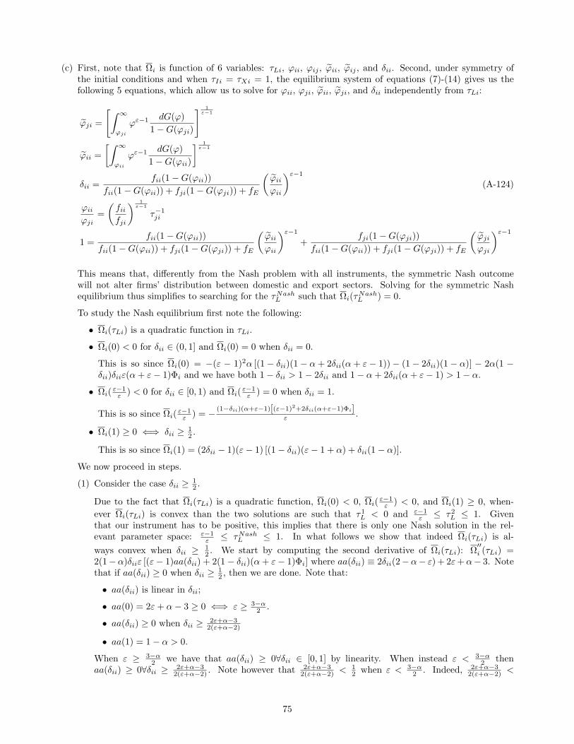
(c) First, note that Ωi is function of 6 variables: τLi, ϕii, ϕij , ϕii, ϕij , and δii. Second, under symmetry ofthe initial conditions and when τIi = τXi = 1, the equilibrium system of equations (7)-(14) gives us thefollowing 5 equations, which allow us to solve for ϕii, ϕji, ϕii, ϕji, and δii independently from τLi:

ϕji =

[∫ ∞

ϕji

ϕε−1 dG(ϕ)

1−G(ϕji)

] 1ε−1

ϕii =

[∫ ∞

ϕii

ϕε−1 dG(ϕ)

1−G(ϕii)

] 1ε−1

δii =fii(1−G(ϕii))


(ϕii

ϕii

)ε−1

(A-124)

ϕii

ϕji=

(fiifji

) 1ε−1

τ−1ji

1 =fii(1−G(ϕii))


(ϕii

ϕii

)ε−1

+fji(1−G(ϕji))


(ϕji

ϕji

)ε−1

This means that, differently from the Nash problem with all instruments, the symmetric Nash outcomewill not alter firms’ distribution between domestic and export sectors. Solving for the symmetric Nashequilibrium thus simplifies to searching for the τNash

L such that Ωi(τNashL ) = 0.

To study the Nash equilibrium first note the following:

• Ωi(τLi) is a quadratic function in τLi.

• Ωi(0) < 0 for δii ∈ (0, 1] and Ωi(0) = 0 when δii = 0.

This is so since Ωi(0) = −(ε − 1)2α [(1− δii)(1− α+ 2δii(α+ ε− 1))− (1− 2δii)(1− α)] − 2α(1 −δii)δiiε(α+ ε− 1)Φi and we have both 1− δii > 1− 2δii and 1− α+ 2δii(α+ ε− 1) > 1− α.

• Ωi(ε−1ε ) < 0 for δii ∈ [0, 1) and Ωi(

ε−1ε ) = 0 when δii = 1.

This is so since Ωi(ε−1ε ) = − (1−δii)(α+ε−1)[(ε−1)2+2δii(α+ε−1)Φi]

ε .

• Ωi(1) ≥ 0 ⇐⇒ δii ≥ 12 .

This is so since Ωi(1) = (2δii − 1)(ε− 1) [(1− δii)(ε− 1 + α) + δii(1− α)].

We now proceed in steps.

(1) Consider the case δii ≥ 12 .

Due to the fact that Ωi(τLi) is a quadratic function, Ωi(0) < 0, Ωi(ε−1ε ) < 0, and Ωi(1) ≥ 0, when-

ever Ωi(τLi) is convex than the two solutions are such that τ1L < 0 and ε−1ε ≤ τ2L ≤ 1. Given

that our instrument has to be positive, this implies that there is only one Nash solution in the rel-evant parameter space: ε−1

ε ≤ τNashL ≤ 1. In what follows we show that indeed Ωi(τLi) is al-

ways convex when δii ≥ 12 . We start by computing the second derivative of Ωi(τLi): Ω

′′

i (τLi) =2(1−α)δiiε [(ε− 1)aa(δii) + 2(1− δii)(α+ ε− 1)Φi] where aa(δii) ≡ 2δii(2−α− ε) + 2ε+α− 3. Notethat if aa(δii) ≥ 0 when δii ≥ 1

2 , then we are done. Note that:

• aa(δii) is linear in δii;

• aa(0) = 2ε+ α− 3 ≥ 0 ⇐⇒ ε ≥ 3−α2 .

• aa(δii) ≥ 0 when δii ≥ 2ε+α−32(ε+α−2)

• aa(1) = 1− α > 0.

When ε ≥ 3−α2 we have that aa(δii) ≥ 0∀δii ∈ [0, 1] by linearity. When instead ε < 3−α

2 thenaa(δii) ≥ 0∀δii ≥ 2ε+α−3

2(ε+α−2) . Note however that 2ε+α−32(ε+α−2) < 1

2 when ε < 3−α2 . Indeed, 2ε+α−3

2(ε+α−2) <

75

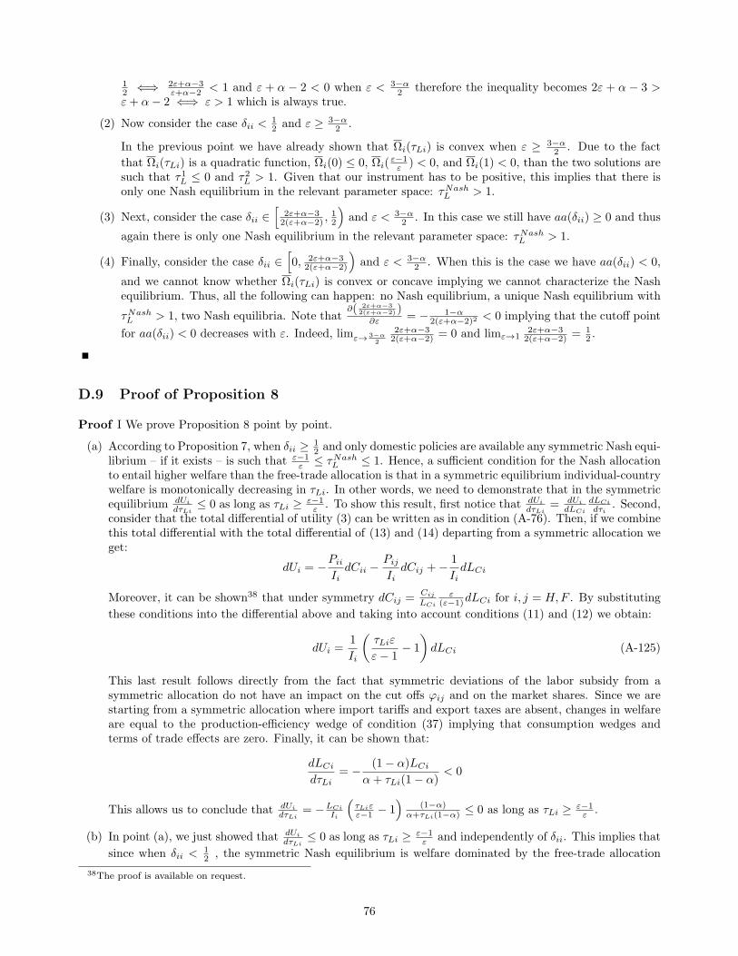
12 ⇐⇒ 2ε+α−3

ε+α−2 < 1 and ε + α − 2 < 0 when ε < 3−α2 therefore the inequality becomes 2ε + α − 3 >

ε+ α− 2 ⇐⇒ ε > 1 which is always true.

(2) Now consider the case δii <12 and ε ≥ 3−α

2 .

In the previous point we have already shown that Ωi(τLi) is convex when ε ≥ 3−α2 . Due to the fact

that Ωi(τLi) is a quadratic function, Ωi(0) ≤ 0, Ωi(ε−1ε ) < 0, and Ωi(1) < 0, than the two solutions are

such that τ1L ≤ 0 and τ2L > 1. Given that our instrument has to be positive, this implies that there isonly one Nash equilibrium in the relevant parameter space: τNash

L > 1.

(3) Next, consider the case δii ∈[

2ε+α−32(ε+α−2) ,

12

)and ε < 3−α

2 . In this case we still have aa(δii) ≥ 0 and thus

again there is only one Nash equilibrium in the relevant parameter space: τNashL > 1.

(4) Finally, consider the case δii ∈[0, 2ε+α−3

2(ε+α−2)

)and ε < 3−α

2 . When this is the case we have aa(δii) < 0,

and we cannot know whether Ωi(τLi) is convex or concave implying we cannot characterize the Nashequilibrium. Thus, all the following can happen: no Nash equilibrium, a unique Nash equilibrium with

τNashL > 1, two Nash equilibria. Note that

∂( 2ε+α−32(ε+α−2) )

∂ε = − 1−α2(ε+α−2)2 < 0 implying that the cutoff point

for aa(δii) < 0 decreases with ε. Indeed, limε→ 3−α2

2ε+α−32(ε+α−2) = 0 and limε→1

2ε+α−32(ε+α−2) =

12 .


Proof I We prove Proposition 8 point by point.

(a) According to Proposition 7, when δii ≥ 12 and only domestic policies are available any symmetric Nash equi-

librium – if it exists – is such that ε−1ε ≤ τNash

L ≤ 1. Hence, a sufficient condition for the Nash allocationto entail higher welfare than the free-trade allocation is that in a symmetric equilibrium individual-countrywelfare is monotonically decreasing in τLi. In other words, we need to demonstrate that in the symmetricequilibrium dUi

dτLi≤ 0 as long as τLi ≥ ε−1

ε . To show this result, first notice that dUi

dτLi= dUi

dLCi

dLCi

dτi. Second,

consider that the total differential of utility (3) can be written as in condition (A-76). Then, if we combinethis total differential with the total differential of (13) and (14) departing from a symmetric allocation weget:

dUi = −Pii

IidCii −

Pij

IidCij +− 1

IidLCi

Moreover, it can be shown38 that under symmetry dCij =Cij

LCi

ε(ε−1)dLCi for i, j = H,F . By substituting

these conditions into the differential above and taking into account conditions (11) and (12) we obtain:

dUi =1

Ii

(τLiε

ε− 1− 1

)dLCi (A-125)

This last result follows directly from the fact that symmetric deviations of the labor subsidy from asymmetric allocation do not have an impact on the cut offs ϕij and on the market shares. Since we arestarting from a symmetric allocation where import tariffs and export taxes are absent, changes in welfareare equal to the production-efficiency wedge of condition (37) implying that consumption wedges andterms of trade effects are zero. Finally, it can be shown that:

dLCi

dτLi= − (1− α)LCi

α+ τLi(1− α)< 0

This allows us to conclude that dUi

dτLi= −LCi

Ii

(τLiεε−1 − 1

)(1−α)

α+τLi(1−α) ≤ 0 as long as τLi ≥ ε−1ε .

(b) In point (a), we just showed that dUi

dτLi≤ 0 as long as τLi ≥ ε−1

ε and independently of δii. This implies that

since when δii < 12 , the symmetric Nash equilibrium is welfare dominated by the free-trade allocation

38The proof is available on request.

76

because of the result from Proposition 8. It is easy to show that when starting from a symmetric allocationcondition (A-125) holds also when firms are homogeneous. Moreover, Campolmi et al. (2014) have alreadyproved that in this case dLCi/dτLi = dNi/dτLi < 0.

(c) By taking the the differential of conditions (7), (8) and (9) with respect to fij and τij , it can be shownthat:

dδii =(ε− 1 + Φi)δii(1− δii)

τijdτij +

Φiδii(1− δii)ϕ1−εij ϕε−1

ij

(ε− 1)fijdfij

which confirms that δii is monotonically increasing in both τij and fij .

77

Documents

Trade and Domestic Policies in Models with Monopolistic