Embed Size (px)
Citation preview

Tracking People and Activities in Video Recordings of
Classroom Presentations
João Nuno Domingos Pacheco
Dissertação para obtenção do Grau de Mestre em
Engenharia Informática e de Computadores
Júri
Presidente: Professora Doutora Ana Maria Severino de Almeida e PaivaOrientador: Professor Doutor Joaquim Armando Pires JorgeCo-Orientador: Professor Doutor Jorge dos Santos Salvador MarquesVogal: Professor Doutor João Paulo Salgado Arriscado Costeira
Novembro 2009

Acknowledgements
I would like to thank my supervisor Prof. Joaquim Jorge for his guidance, ideas, enthusiasm, exigency and for
keeping me focused on the essential.
I also would like to thank my supervisor Prof. Salvador Marques for his very useful advices, explanation
and discussion of alternative solutions, and support on improving the solution.
A special thanks to Tiago Costa for his kind collaboration in providing the first test video sequences and
information about the video acquisition conditions.
I would like to thank André Martins for providing some needed resources to work with, and Bruno Araújo
and Ricardo Jota for showing their support in camera handling and OpenCV use. Prof. José Gaspar was
also helpful on explaining how to handle and remove distortion caused by camera lenses, which may be con-
sidered in a future improvement of this work. I would like to thank Inês Gonçalves for her help on statistics
and support on other issues. I also would like to thank Pedro Marques for making some suggestions and
questions which helped clarifying the content.
A very special thanks to the experts who patiently and courageously labeled the data set.
I would like to thank to my course colleagues João Freitas, Nelson Alves, Eurico Doirado and many oth-
ers with whom I was able to learn many valuable things to use in the present work.
I would also like to thank all the people that share their knowledge on this work’s domain in the Internet
and those that contribute to open source tools such as OpenCV. Their work saved me time which was used
to focus on more advanced problems.
My family and friends deserve a special thanks for their generous support, motivation, patience, for being
understanding and for enabling a peaceful environment so I could focus on the work in hands.
Finally, I must thank Ofélia for being so understanding and encouraging, for her endless support and mo-
tivation, and for her useful suggestions for improvements.
Thank you all, you made a high positive contribution.
i

Abstract
Interactive presentations are a very significant way of sharing knowledge between people. Nowadays, trans-
mitting effectively a complex idea to others may require technological advanced tools, such as virtual tables
and specialized software, although most of them simply rely on slide shows. By evaluating the interactions
between people in presentations, the speaker(s) or the other participants may perceive their flaws and im-
prove their communication strategy. Reducing costs in recording presentations is also a requirement.
The goals of this thesis are developing a real time system to recognize a set of activities performed by the
presentation speaker and record the presentation; developing a suitable human tracker to the presentation
environment; and designing a generic and extensible architecture for human activity recognition.
This dissertation presents a real time system for human activity recognition and video recording, applied to the
interactive presentation environment. The developed tracking algorithm considerably supports different indoor
illumination conditions, tracks the speaker in both frontal and side views, and adapts to body scale. Speaker’s
face and hand regions are obtained by tracking skin regions and torso vertical boundaries are given by the
median edge points. The activity classifiers were trained with SVM and Normal Bayes and their recall rates
vary from 10 to 86.67%. It was shown that the classifiers recognize a high number of activity occurrences, but
they are split into small occurrences, leading to a low performance. Conclusions state the need of enhancing
tracking robustness and experimenting the classifiers parameters to improve their performance.
Keywords: Interactive presentation, human activity recognition, human tracking, automatic video recording
ii

Resumo
As apresentações interactivas são uma forma bastante eficaz de partilhar conhecimento entre pessoas.
Actualmente, explicar eficazmente uma ideia complexa a outros pode exigir tecnologia avançada, embora
a maioria ainda se limite a utilizar slides. Ao avaliar as interacções entre as pessoas nas apresentações, os
vários participantes podem aperceber-se das suas falhas e melhorar a sua estratégia de comunicação. Outra
necessidade é a redução de custos na gravação das apresentações.
Os objectivos desta tese são desenvolver um sistema em tempo real para reconhecer um conjunto de ac-
tividades efectuadas pelo orador e gravar a apresentação; desenvolver um seguidor adequado ao ambiente
da apresentação; e desenhar uma arquitectura genérica e extensível para reconhecimento de actividades
humanas.
Esta dissertação apresenta um sistema para reconhecimento de actividades humanas e gravação de vídeo,
aplicado ao ambiente da apresentação interactiva. O algoritmo de seguimento de suporte ao sistema fun-
ciona com diferentes condições de iluminação, segue o orador nas vistas frontal e lateral, e adapta-se à
escala do orador. As regiões da face e mãos são obtidas ao seguir as regiões de pele e os limites verticais
do tronco correspondem à mediana dos pontos de contorno. Os classificadores de actividades treinados
com SVM e Normal Bayes atingiram taxas de recall que variam entre 10% e 86.67%. Observou-se que
os classificadores reconhecem um elevado número das ocorrências de actividade, mas estas são partidas
em pequenas ocorrências levando a um menor desempenho. Concluiu-se a necessidade de aumentar a
robustez do seguimento e de testar os classificadores com novos parâmetros.
Palavras-chave: Apresentação interactiva, reconhecimento de actividades humanas, seguimento de
pessoas, gravação automática de vídeo
iii
Contents
List of Tables vii
List of Figures ix
1 Introduction 1
1.1 Motivation . . . . . . . . . . . . . . . . . . . . . . . . . . . . . . . . . . . . . . . . . . . . . . 1
1.2 Interactive Presentation . . . . . . . . . . . . . . . . . . . . . . . . . . . . . . . . . . . . . . . 1
1.3 Problem Overview . . . . . . . . . . . . . . . . . . . . . . . . . . . . . . . . . . . . . . . . . . 2
1.4 Goals and Success Criteria . . . . . . . . . . . . . . . . . . . . . . . . . . . . . . . . . . . . . 2
1.5 Results . . . . . . . . . . . . . . . . . . . . . . . . . . . . . . . . . . . . . . . . . . . . . . . . 3
1.6 Contributions . . . . . . . . . . . . . . . . . . . . . . . . . . . . . . . . . . . . . . . . . . . . 3
1.7 Dissertation Outline . . . . . . . . . . . . . . . . . . . . . . . . . . . . . . . . . . . . . . . . . 4
2 State of the Art 5
2.1 Introduction . . . . . . . . . . . . . . . . . . . . . . . . . . . . . . . . . . . . . . . . . . . . . 5
2.2 Interactive Presentations . . . . . . . . . . . . . . . . . . . . . . . . . . . . . . . . . . . . . . 5
2.2.1 Tools . . . . . . . . . . . . . . . . . . . . . . . . . . . . . . . . . . . . . . . . . . . . . 5
2.2.2 Previous Work . . . . . . . . . . . . . . . . . . . . . . . . . . . . . . . . . . . . . . . . 6
2.3 Human Representation . . . . . . . . . . . . . . . . . . . . . . . . . . . . . . . . . . . . . . . 7
2.4 Human Detection and Tracking . . . . . . . . . . . . . . . . . . . . . . . . . . . . . . . . . . . 7
2.4.1 Segmentation . . . . . . . . . . . . . . . . . . . . . . . . . . . . . . . . . . . . . . . . 7
2.4.2 Tracking . . . . . . . . . . . . . . . . . . . . . . . . . . . . . . . . . . . . . . . . . . . 10
2.4.3 Skin Detection . . . . . . . . . . . . . . . . . . . . . . . . . . . . . . . . . . . . . . . . 11
2.4.4 Face detection . . . . . . . . . . . . . . . . . . . . . . . . . . . . . . . . . . . . . . . . 13
2.5 Human Activity Recognition . . . . . . . . . . . . . . . . . . . . . . . . . . . . . . . . . . . . . 14
2.5.1 Common Detected Activities and Events . . . . . . . . . . . . . . . . . . . . . . . . . . 14
2.5.2 Main Features . . . . . . . . . . . . . . . . . . . . . . . . . . . . . . . . . . . . . . . . 14
2.5.3 Algorithms for Classification . . . . . . . . . . . . . . . . . . . . . . . . . . . . . . . . 14
2.6 Discussion . . . . . . . . . . . . . . . . . . . . . . . . . . . . . . . . . . . . . . . . . . . . . . 14
2.6.1 Interactive Presentations and Meetings . . . . . . . . . . . . . . . . . . . . . . . . . . 15
2.6.2 Human Representation . . . . . . . . . . . . . . . . . . . . . . . . . . . . . . . . . . . 15
2.6.3 Segmentation . . . . . . . . . . . . . . . . . . . . . . . . . . . . . . . . . . . . . . . . 15
2.6.4 Tracking . . . . . . . . . . . . . . . . . . . . . . . . . . . . . . . . . . . . . . . . . . . 16
2.6.5 Skin Detection . . . . . . . . . . . . . . . . . . . . . . . . . . . . . . . . . . . . . . . . 16
2.6.6 Face Detection . . . . . . . . . . . . . . . . . . . . . . . . . . . . . . . . . . . . . . . 16
2.6.7 Human Activity Recognition . . . . . . . . . . . . . . . . . . . . . . . . . . . . . . . . . 17
2.7 Conclusions . . . . . . . . . . . . . . . . . . . . . . . . . . . . . . . . . . . . . . . . . . . . . 17
iv
3 Problem Formulation 18
3.1 Introduction . . . . . . . . . . . . . . . . . . . . . . . . . . . . . . . . . . . . . . . . . . . . . 18
3.2 Activity Scenarios . . . . . . . . . . . . . . . . . . . . . . . . . . . . . . . . . . . . . . . . . . 18
3.2.1 Current Activity Scenario . . . . . . . . . . . . . . . . . . . . . . . . . . . . . . . . . . 18
3.2.2 Desired Activity Scenario . . . . . . . . . . . . . . . . . . . . . . . . . . . . . . . . . . 19
3.3 Problem Description . . . . . . . . . . . . . . . . . . . . . . . . . . . . . . . . . . . . . . . . . 19
3.3.1 Detect and Track the Speaker . . . . . . . . . . . . . . . . . . . . . . . . . . . . . . . 19
3.3.2 Recognizing Speaker Activities . . . . . . . . . . . . . . . . . . . . . . . . . . . . . . . 20
3.3.3 Recording Presentation . . . . . . . . . . . . . . . . . . . . . . . . . . . . . . . . . . . 21
3.4 Discussion . . . . . . . . . . . . . . . . . . . . . . . . . . . . . . . . . . . . . . . . . . . . . . 21
4 Intelligent Recording System 22
4.1 Introduction . . . . . . . . . . . . . . . . . . . . . . . . . . . . . . . . . . . . . . . . . . . . . 22
4.2 Tracking Algorithm . . . . . . . . . . . . . . . . . . . . . . . . . . . . . . . . . . . . . . . . . . 22
4.2.1 Background Subtraction . . . . . . . . . . . . . . . . . . . . . . . . . . . . . . . . . . . 24
4.2.2 Face . . . . . . . . . . . . . . . . . . . . . . . . . . . . . . . . . . . . . . . . . . . . . 26
4.2.3 Torso . . . . . . . . . . . . . . . . . . . . . . . . . . . . . . . . . . . . . . . . . . . . . 34
4.2.4 Hands . . . . . . . . . . . . . . . . . . . . . . . . . . . . . . . . . . . . . . . . . . . . 36
4.3 Recognizing Activities . . . . . . . . . . . . . . . . . . . . . . . . . . . . . . . . . . . . . . . . 39
4.3.1 Characterizing Activities . . . . . . . . . . . . . . . . . . . . . . . . . . . . . . . . . . . 40
4.3.2 Classification Algorithms . . . . . . . . . . . . . . . . . . . . . . . . . . . . . . . . . . 44
4.3.3 Train and Test . . . . . . . . . . . . . . . . . . . . . . . . . . . . . . . . . . . . . . . . 46
4.4 Video Recording . . . . . . . . . . . . . . . . . . . . . . . . . . . . . . . . . . . . . . . . . . . 47
4.5 Discussion . . . . . . . . . . . . . . . . . . . . . . . . . . . . . . . . . . . . . . . . . . . . . . 47
4.5.1 Image Resolution and Scalability . . . . . . . . . . . . . . . . . . . . . . . . . . . . . . 48
4.5.2 Processed Frames . . . . . . . . . . . . . . . . . . . . . . . . . . . . . . . . . . . . . 48
4.5.3 Human Proportions . . . . . . . . . . . . . . . . . . . . . . . . . . . . . . . . . . . . . 48
4.5.4 Background Subtraction . . . . . . . . . . . . . . . . . . . . . . . . . . . . . . . . . . . 48
4.5.5 Skin Detection . . . . . . . . . . . . . . . . . . . . . . . . . . . . . . . . . . . . . . . . 48
4.5.6 Body Tracking . . . . . . . . . . . . . . . . . . . . . . . . . . . . . . . . . . . . . . . . 50
4.5.7 Activity Recognition . . . . . . . . . . . . . . . . . . . . . . . . . . . . . . . . . . . . . 53
4.5.8 Capabilities and Limitations . . . . . . . . . . . . . . . . . . . . . . . . . . . . . . . . . 53
4.5.9 Technology . . . . . . . . . . . . . . . . . . . . . . . . . . . . . . . . . . . . . . . . . . 54
4.6 Conclusions . . . . . . . . . . . . . . . . . . . . . . . . . . . . . . . . . . . . . . . . . . . . . 55
5 Experimental Results 56
5.1 Introduction . . . . . . . . . . . . . . . . . . . . . . . . . . . . . . . . . . . . . . . . . . . . . 56
5.2 Video Data Set . . . . . . . . . . . . . . . . . . . . . . . . . . . . . . . . . . . . . . . . . . . 56
5.2.1 Illumination and Room Characteristics . . . . . . . . . . . . . . . . . . . . . . . . . . . 56
5.2.2 Data Labeling . . . . . . . . . . . . . . . . . . . . . . . . . . . . . . . . . . . . . . . . 57
5.2.3 Training and Test Sets . . . . . . . . . . . . . . . . . . . . . . . . . . . . . . . . . . . . 60
5.3 Tracking Evaluation . . . . . . . . . . . . . . . . . . . . . . . . . . . . . . . . . . . . . . . . . 60
5.3.1 Evaluation Metrics . . . . . . . . . . . . . . . . . . . . . . . . . . . . . . . . . . . . . . 60
5.3.2 Tracking Performance . . . . . . . . . . . . . . . . . . . . . . . . . . . . . . . . . . . . 61
5.3.3 Tracking Performance in Non-constant Illumination . . . . . . . . . . . . . . . . . . . . 62
5.4 Activity Recognition Evaluation . . . . . . . . . . . . . . . . . . . . . . . . . . . . . . . . . . . 64
5.4.1 Recognition Metrics . . . . . . . . . . . . . . . . . . . . . . . . . . . . . . . . . . . . . 64
v

5.4.2 Results of Activity Classifiers . . . . . . . . . . . . . . . . . . . . . . . . . . . . . . . . 64
5.5 Speed Evaluation . . . . . . . . . . . . . . . . . . . . . . . . . . . . . . . . . . . . . . . . . . 75
5.6 Discussion . . . . . . . . . . . . . . . . . . . . . . . . . . . . . . . . . . . . . . . . . . . . . . 77
5.7 Conclusions . . . . . . . . . . . . . . . . . . . . . . . . . . . . . . . . . . . . . . . . . . . . . 78
6 Conclusions 79
6.1 Work Review . . . . . . . . . . . . . . . . . . . . . . . . . . . . . . . . . . . . . . . . . . . . . 79
6.2 Future Work . . . . . . . . . . . . . . . . . . . . . . . . . . . . . . . . . . . . . . . . . . . . . 80
Bibliography 81
A Features 89
B Video Data Set 90
C Tracker Experimental Results 95
D Speed Measurements 102
vi

List of Tables
1.1 Best precision and recall rates for each activity . . . . . . . . . . . . . . . . . . . . . . . . . . 3
2.1 Comparison of systems for the smart room environment . . . . . . . . . . . . . . . . . . . . . 15
4.1 Feature set of activity A . . . . . . . . . . . . . . . . . . . . . . . . . . . . . . . . . . . . . . . 40
4.2 Feature set of activity B . . . . . . . . . . . . . . . . . . . . . . . . . . . . . . . . . . . . . . . 40
4.3 Feature set of activity C . . . . . . . . . . . . . . . . . . . . . . . . . . . . . . . . . . . . . . . 42
4.4 Feature set of activities E and F . . . . . . . . . . . . . . . . . . . . . . . . . . . . . . . . . . 43
5.1 Average tracking performance of the speaker’s face for Group 1. . . . . . . . . . . . . . . . . . 61
5.2 Average tracking performance of the speaker’s torso for Group 1. . . . . . . . . . . . . . . . . 62
5.3 Average tracking performance of the speaker’s left hand for Group 1. . . . . . . . . . . . . . . 62
5.4 Average tracking performance of the speaker’s right hand for Group 1. . . . . . . . . . . . . . 62
5.5 Average tracking performance of the speaker’s face for Group 2. . . . . . . . . . . . . . . . . . 63
5.6 Average tracking performance of the speaker’s torso for Group 1. . . . . . . . . . . . . . . . . 63
5.7 Average tracking performance of the speaker’s left hand for Group 2. . . . . . . . . . . . . . . 63
5.8 Average tracking performance of the speaker’s right hand for Group 2. . . . . . . . . . . . . . 64
5.9 Best results for each activity classifier . . . . . . . . . . . . . . . . . . . . . . . . . . . . . . . 74
5.10 Tracker’s average speed for three image resolutions . . . . . . . . . . . . . . . . . . . . . . . 77
5.11 System’s average speed over three image resolutions . . . . . . . . . . . . . . . . . . . . . . 77
A.1 List of features used for activity recognition . . . . . . . . . . . . . . . . . . . . . . . . . . . . 89
B.1 Test set video sequences for tracking (Group 1) . . . . . . . . . . . . . . . . . . . . . . . . . . 90
B.2 Test set for tracking under different illumination conditions (Group 2) . . . . . . . . . . . . . . . 90
B.3 Training set for activities (A and B) . . . . . . . . . . . . . . . . . . . . . . . . . . . . . . . . . 92
B.4 Training set for activities (C and D) . . . . . . . . . . . . . . . . . . . . . . . . . . . . . . . . . 93
B.5 Training set for activities (E and F) . . . . . . . . . . . . . . . . . . . . . . . . . . . . . . . . . 94
C.1 Tracker’s performance for speaker’s face (90x72) . . . . . . . . . . . . . . . . . . . . . . . . . 95
C.2 Tracker’s performance for speaker’s torso (90x72) . . . . . . . . . . . . . . . . . . . . . . . . . 95
C.3 Tracker’s performance for speaker’s left hand (90x72) . . . . . . . . . . . . . . . . . . . . . . . 95
C.4 Tracker’s performance for speaker’s right hand (90x72) . . . . . . . . . . . . . . . . . . . . . . 96
C.5 Tracker’s performance for speaker’s face (180x144) . . . . . . . . . . . . . . . . . . . . . . . . 96
C.6 Tracker’s performance for speaker’s torso . . . . . . . . . . . . . . . . . . . . . . . . . . . . . 96
C.7 Tracker’s performance for speaker’s left hand (180x144) . . . . . . . . . . . . . . . . . . . . . 96
C.8 Tracker’s performance for speaker’s right hand (180x144) . . . . . . . . . . . . . . . . . . . . 97
C.9 Tracker’s performance for speaker’s face (360x288) . . . . . . . . . . . . . . . . . . . . . . . . 97
C.10 Tracker’s performance for speaker’s torso (360x288) . . . . . . . . . . . . . . . . . . . . . . . 97
vii
C.11 Tracker’s performance for speaker’s left hand (360x288) . . . . . . . . . . . . . . . . . . . . . 97
C.12 Tracker’s performance for speaker’s right hand (360x288) . . . . . . . . . . . . . . . . . . . . 98
C.13 Tracker’s performance for speaker’s face (90x72) . . . . . . . . . . . . . . . . . . . . . . . . . 98
C.14 Tracker’s performance for speaker’s torso (90x72) . . . . . . . . . . . . . . . . . . . . . . . . . 98
C.15 Tracker’s performance for speaker’s left hand (90x72) . . . . . . . . . . . . . . . . . . . . . . . 98
C.16 Tracker’s performance for speaker’s right hand (90x72) . . . . . . . . . . . . . . . . . . . . . . 99
C.17 Tracker’s performance for speaker’s face (180x144) . . . . . . . . . . . . . . . . . . . . . . . . 99
C.18 Tracker’s performance for speaker’s torso (180x144) . . . . . . . . . . . . . . . . . . . . . . . 99
C.19 Tracker’s performance for speaker’s left hand (180x144) . . . . . . . . . . . . . . . . . . . . . 100
C.20 Tracker’s performance for speaker’s right hand (180x144) . . . . . . . . . . . . . . . . . . . . 100
C.21 Tracker’s performance for speaker’s face (360x288) . . . . . . . . . . . . . . . . . . . . . . . . 100
C.22 Tracker’s performance for speaker’s torso (360x288) . . . . . . . . . . . . . . . . . . . . . . . 100
C.23 Tracker’s performance for speaker’s left hand (360x288) . . . . . . . . . . . . . . . . . . . . . 101
C.24 Tracker’s performance for speaker’s right hand (360x288) . . . . . . . . . . . . . . . . . . . . 101
D.1 Tracker’s speed over three image resolutions . . . . . . . . . . . . . . . . . . . . . . . . . . . 102
D.2 System’s speed over three image resolutions . . . . . . . . . . . . . . . . . . . . . . . . . . . 102
viii

List of Figures
4.1 Architecture of the system . . . . . . . . . . . . . . . . . . . . . . . . . . . . . . . . . . . . . 23
4.2 Human body model and its proportions . . . . . . . . . . . . . . . . . . . . . . . . . . . . . . 24
4.3 Image coordinates system . . . . . . . . . . . . . . . . . . . . . . . . . . . . . . . . . . . . . 25
4.4 Example of the binary images (1) . . . . . . . . . . . . . . . . . . . . . . . . . . . . . . . . . 27
4.5 Example of the binary images (2) . . . . . . . . . . . . . . . . . . . . . . . . . . . . . . . . . 28
4.6 Example of the binary images (3) . . . . . . . . . . . . . . . . . . . . . . . . . . . . . . . . . 29
4.7 Example of face detection with skin blobs. . . . . . . . . . . . . . . . . . . . . . . . . . . . . . 30
4.8 Number of tracker initializations for each β5 value . . . . . . . . . . . . . . . . . . . . . . . . . 32
4.9 Example of a binary skin map and its corresponding labels. . . . . . . . . . . . . . . . . . . . 34
4.10 Example of the torso detection. . . . . . . . . . . . . . . . . . . . . . . . . . . . . . . . . . . . 35
4.11 Regions around the speaker where hand blobs are searched. . . . . . . . . . . . . . . . . . . 37
4.12 Examples of the activity A (“Speaker has bent”) . . . . . . . . . . . . . . . . . . . . . . . . . . 41
4.13 Examples of the activity B (“Speaker’s face is visible”) . . . . . . . . . . . . . . . . . . . . . . 41
4.14 Examples of activity C (“Speaker is pointing to his/her left”). . . . . . . . . . . . . . . . . . . . 42
4.15 Examples of the activity D (“Speaker is pointing to his/her right”) . . . . . . . . . . . . . . . . . 42
4.16 Examples of the activity E (“Speaker has moved to his/her left”) . . . . . . . . . . . . . . . . . 43
4.17 Example of a separable problem with SVM. . . . . . . . . . . . . . . . . . . . . . . . . . . . . 45
4.18 Example of the recorded images in every frame. . . . . . . . . . . . . . . . . . . . . . . . . . 47
4.19 Skin detection performance using several skin classifiers . . . . . . . . . . . . . . . . . . . . . 49
4.20 Results of four torso tracking techniques . . . . . . . . . . . . . . . . . . . . . . . . . . . . . . 51
4.21 Results of four torso tracking techniques . . . . . . . . . . . . . . . . . . . . . . . . . . . . . . 52
5.1 Example of a human labeling . . . . . . . . . . . . . . . . . . . . . . . . . . . . . . . . . . . . 57
5.2 Interface of the program to collect the tracker’s GT . . . . . . . . . . . . . . . . . . . . . . . . 58
5.3 Counterexample of activity D . . . . . . . . . . . . . . . . . . . . . . . . . . . . . . . . . . . . 59
5.4 Program used to observe the activity occurrences . . . . . . . . . . . . . . . . . . . . . . . . 59
5.5 Performance of the classifiers for activity A (K = 6). . . . . . . . . . . . . . . . . . . . . . . . 66
5.6 Performance of the classifiers for activity A . . . . . . . . . . . . . . . . . . . . . . . . . . . . 67
5.7 Example of activity A splitting. . . . . . . . . . . . . . . . . . . . . . . . . . . . . . . . . . . . 67
5.8 Performance of the classifiers for activity B . . . . . . . . . . . . . . . . . . . . . . . . . . . . 68
5.9 Examples of error causes in recognizing activity B. . . . . . . . . . . . . . . . . . . . . . . . . 68
5.10 Examples of activity B estimations. . . . . . . . . . . . . . . . . . . . . . . . . . . . . . . . . . 69
5.11 Performance of the classifiers for activity C . . . . . . . . . . . . . . . . . . . . . . . . . . . . 70
5.12 Examples of FP of activity C. . . . . . . . . . . . . . . . . . . . . . . . . . . . . . . . . . . . . 70
5.13 Examples of activity C estimations. . . . . . . . . . . . . . . . . . . . . . . . . . . . . . . . . . 71
5.14 Similar activity to C. . . . . . . . . . . . . . . . . . . . . . . . . . . . . . . . . . . . . . . . . . 71
5.15 Performance of the classifiers for activity D . . . . . . . . . . . . . . . . . . . . . . . . . . . . 72
ix

5.16 Examples of activity D estimations. . . . . . . . . . . . . . . . . . . . . . . . . . . . . . . . . . 73
5.17 Similar activity to D. . . . . . . . . . . . . . . . . . . . . . . . . . . . . . . . . . . . . . . . . . 73
5.18 Performance of the classifiers for activity E . . . . . . . . . . . . . . . . . . . . . . . . . . . . 74
5.19 Examples of activity E estimations. . . . . . . . . . . . . . . . . . . . . . . . . . . . . . . . . . 75
5.20 Performance of the classifiers for activity F . . . . . . . . . . . . . . . . . . . . . . . . . . . . 76
5.21 Examples of activity F estimations. . . . . . . . . . . . . . . . . . . . . . . . . . . . . . . . . . 76
B.1 Examples of the presentation rooms . . . . . . . . . . . . . . . . . . . . . . . . . . . . . . . . 91
x

List of AcronymsCV - Computer Vision
PTZ - Pan-tilt-zoom
BS - Background Subtraction
SVM - Support Vector Machines
HMM - Hidden Markov Models
ANN - Artificial Neural Networks
FPS - Frames per second
GT - Ground Truth
FP - False Positives
FN - False Negatives
xi

Chapter 1
Introduction
1.1 MotivationNowadays, many interactive presentations are given all over the world, whether in academic classrooms,
business meetings or scientific conferences. It would be interesting and useful that we could record in video
and audio what happened in them for later viewing. For students, recorded classes would be useful so they
could watch them, whether they were or not present, playing them at their own pace of learning [Schn 96].
Furthermore, students attending distance courses would consider this essential to their learning, as well as
those who wish to learn more about a particular topic. Also in industrial training, recorded presentations given
to each human resource would be cheaper and easier than joining some human resources and scheduling
some hours to give them a live presentation. Besides, this presentation could be reused in the future.
International conferences on sciences could also be recorded and sold to interested users, as it is already
being done with the published articles. We can see that a recorded multi-view presentation, that includes the
speaker and audience images/audio, and its slide show, is a fast and cheap way of sharing knowledge. An
example of knowledge sharing are the educational videos on Youtube [Hurl 09], which includes thousands of
university lectures.
Recognizing events (or activities) in video may be useful to automatically segment the presentation into sev-
eral videos, according to the entry and exit of the speaker in the image’s field of view, or according to other
specific events. Since each speaker has a specific style to make presentations, his/her set of activities may be
used to distinguish between speakers. In courses where people take lessons on making public presentations,
an activity recognition system may be applied to analyze each student’s behaviors, so they become aware
of unsuitable behaviors and improve their non-verbal communication. Additionally, recognizing activities on
videos may be used to label them by their content and subsequently a video may be retrieved by searching
its labels.
To record interactive presentations we must have at least one camera, at least one microphone and tech-
nical staff that operates each camera and/or microphone. This sounds expensive and it is. Therefore, what
we desire is an automated and intelligent system that, once it is easily manually configured, records in video
the speaker and part of the audience, and provides information about the presentation events by recognizing
some of the speaker’s activities. Such a system significantly reduces the number of people involved in the
recording process and also reduces the effort required to obtain the presentation recording.
1.2 Interactive PresentationThe work described in this dissertation comes within the context of interactive presentations, which leads to
the need of defining what an interactive presentation is.
1

An interactive presentation is a type of presentation where some kind of subject is exposed for a limited
period of time, to an audience. An interactive presentation could include one or more speakers and it is often
supported by a slide show which contains multimedia objects (text, video, images, audio, graphics). In inter-
active presentations, there should be some interaction between the speaker and the people in the audience,
by speaking or using interaction tools.
1.3 Problem OverviewThis thesis focuses on three main problems. The first problem is the detection and tracking of speaker’s body
parts (face/head, torso and hands) within a classroom. The speaker always moves in an indoor scene, but
there are many changes in lighting, the audience moves and there are body occlusions. These factors make
speaker tracking a difficult task.
The second problem is recognizing a set of activities that the speaker performs. Recognizing these activ-
ities heavily depends on the ability of the tracker to track speaker’s body parts (first problem). Assuming
the tracker is reliable, activity recognition requires analyzing several frames, in order to understand speaker
movements over the time.
The third problem is recording the presentation into two video files. One video contains the presentation
global view, and the another contains a clipped view of the speaker, taken from the global view.
1.4 Goals and Success CriteriaThe goals of this thesis are the following:
• Develop a suitable human tracker to the presentation environment. When developing the tracking algo-
rithm, it was assumed that it would be a single person tracker, the speaker is standing, his/her face and
torso are at least partially visible, the speaker is the only person facing the camera, there would not be
skin-like objects around the speaker and that people from audience are always sit. There may occur
changes in lighting and audience movements should be ignored while focusing on the speaker’s body.
The achievement of this goal is required to accomplish the goals below.
• Analyze the activities characteristics and design a generic and extensible architecture for human ac-
tivity recognition. Attaining this goal requires understanding each activity’s duration and basic motion
characteristics, and also the classification algorithm’s suitability to recognize each activity. Moreover,
one assumed that each activity should be recognized by a previously trained classifier based on visual
features extracted from the tracker’s output. Knowledge about activities characteristics is also useful to
obtain the most suitable features for recognition. Since presentations contain many interesting activi-
ties, a generic and extensible architecture is essential to allow the addition of new activities, features
and classification algorithms.
• Develop a real-time system that recognizes a predefined set of activities performed by the presentation
speaker, and records the presentation on video. This is the main goal of this thesis and involves the
main requirements of the system. This goal depends on the accomplishment of the previous two. It
requires the use of effective but also fast algorithms, in order to perform all the system’s functionalities
in real time.
The success criteria of this thesis are the following:
2
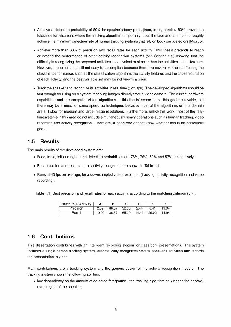
• Achieve a detection probability of 80% for speaker’s body parts (face, torso, hands). 80% provides a
tolerance for situations where the tracking algorithm temporarily loses the face and attempts to roughly
achieve the minimum detection rate of human tracking systems that rely on body part detectors [Mici 05].
• Achieve more than 60% of precision and recall rates for each activity. This thesis pretends to reach
or exceed the performance of other activity recognition systems (see Section 2.5) knowing that the
difficulty in recognizing the proposed activities is equivalent or simpler than the activities in the literature.
However, this criterion is still not easy to accomplish because there are several variables affecting the
classifier performance, such as the classification algorithm, the activity features and the chosen duration
of each activity, and the best variable set may be not known a priori.
• Track the speaker and recognize its activities in real time (>25 fps). The developed algorithms should be
fast enough for using on a system receiving images directly from a video camera. The current hardware
capabilities and the computer vision algorithms in this thesis’ scope make this goal achievable, but
there may be a need for some speed up techniques because most of the algorithms on this domain
are still slow for medium and large image resolutions. Furthermore, unlike this work, most of the real-
timesystems in this area do not include simultaneously heavy operations such as human tracking, video
recording and activity recognition. Therefore, a priori one cannot know whether this is an achievable
goal.
1.5 ResultsThe main results of the developed system are:
• Face, torso, left and right hand detection probabilities are 76%, 76%, 52% and 57%, respectively;
• Best precision and recall rates in activity recognition are shown in Table 1.1;
• Runs at 43 fps on average, for a downsampled video resolution (tracking, activity recognition and video
recording).
Table 1.1: Best precision and recall rates for each activity, according to the matching criterion (5.7).
Rates (%) / Activity A B C D E FPrecision 2.39 86.67 32.50 2.44 6.41 19.04
Recall 10.00 86.67 65.00 14.43 29.02 14.94
1.6 ContributionsThis dissertation contributes with an intelligent recording system for classroom presentations. The system
includes a single person tracking system, automatically recognizes several speaker’s activities and records
the presentation in video.
Main contributions are a tracking system and the generic design of the activity recognition module. The
tracking system shows the following abilities:
• low dependency on the amount of detected foreground - the tracking algorithm only needs the approxi-
mate region of the speaker;
3

• robust to other moving people besides the speaker, provided that the tracker keeps tracking the speaker’s
body parts or people are not close to the speaker - once the speaker is being tracked, the algorithm
ignores the remaining image regions;
• frontal and side tracking of the body parts and scale adaptation - the speaker is tracked in both views
by adapting the current body regions from the previous regions;
• tolerant to variations in the room illumination, unless there is very high or very low lighting - the tracking
algorithm depends on skin detection which is affected by illumination;
• tolerant to speaker’s slow or fast movements - the algorithm may be easily tuned to track fast movements
of face and hands by increasing their search region and using a function for body part similarity.
Activity recognition module was designed so that one can easily add new activities, new features or clas-
sification algorithms. Therefore, the number of recognized activities may be extended with low effort. The
developed system has also been presented in RecPad2009 (www.ieeta.pt/recpad2009).
1.7 Dissertation OutlineThis dissertation is organized in six chapters as follows:
• Chapter 1 - Introduction
Introduces the thesis motivation, defines the interactive presentation concept and provides an overview
of the problem. The chapter also presents the thesis goals, the results achieved and the main contribu-
tions.
• Chapter 2 - State of the Art
Reviews the literature on interactive presentations, human representation, human tracking and human
activity recognition.
• Chapter 3 - Problem Formulation
Introduces the problem statement through two activity scenarios: current scenario and target scenario.
Describes in detail the addressed problem and its requirements.
• Chapter 4 - Intelligent Recording System
Describes the system architecture and details each of its components. It discusses the taken approach
and also the alternative approaches. This chapter also presents an analysis on the system scalability
in space and time, lists the system capabilities and limitations, and discusses the technology choices.
• Chapter 5 - Experimental Results
Presents the experimental results on the performed tests. The first test measures the tracker perfor-
mance under different presentations and speakers. The second test measures the tracker performance
under different illumination conditions of the room. The third test measures the activity classifiers perfor-
mance. The fourth test provides a speed evaluation of the tracking algorithm and the complete system.
This chapter also describes the video data set used and discusses the obtained results.
• Chapter 6 - Conclusions
Provides a summary on the developed work and presents the main conclusions. At the end, some
points on the future work are suggested.
4

Chapter 2
State of the Art
2.1 IntroductionThis chapter covers the state of the art about interactive presentations and enabling technologies, in order to
improve the presentation experience. Related environments to interactive presentations are smart rooms and
video conferences (see Section 2.2).
State of the art of this thesis involves several concepts and techniques from the computer vision (CV) area,
more specifically human representation, human tracking, skin detection and human activity recognition on
video. In this chapter, these are reviewed in Sections 2.3-2.5. Later, a comparative analysis of the reviewed
literature is presented (Section 2.6).
2.2 Interactive PresentationsPeople are the main elements of interactive presentations and meetings. However, other elements are part
of them and have become available to provide a richer experience to the participants. These elements are
tools, such as laser pointers or computers, that the speaker and sometimes the audience use. Next section
presents the tools used in interactive presentations and the later section reviews some systems which have
been developed specifically to operate in interactive presentations or meetings.
2.2.1 ToolsWith the emergence of new technologies, interactive presentations have been integrating new tools to facili-
tate communication between the speaker and the audience. Simultaneously, interaction between people is im-
proved. These tools can be hardware and software. As examples of the slide controlling, there are laser point-
ers [Zhan 08], mobile phones with cameras [Adle 07], and the speaker’s hands [Baud 93, Cao 05, Hard 01],
besides the standard keyboard and mouse. In software, also known as presentation authoring tools, there are
many available solutions. There are standard products such as Microsoft PowerPoint [Micr 09] and Impress
from OpenOffice.org [Inc 09], but these assume a single display and speaker, and do not support multi-display
presentations [Zhan 04]. In addition to these, other authoring tools assume the existence of more than one
display [Zhan 04, Chiu 03]. In [Chiu 03], a group of slides can be shown and each slide is changed by per-
forming gestures on the touch screen where the slide is being shown. In [Zhan 04], PreAuthor is able to create
a multi-channel presentation by using ”hyper-slides” to each output device. It also supports ”hyper-slide” syn-
chronization between each device and distribution of independent ”hyper-slides” to local and remote devices.
In order to improve and overcome the existing authoring tools, several studies have been conducted, re-
sulting in proposals for systems and models of synchronization and management of the multimedia objects
[Schn 96, Ko 95, Kuo 97]. With the improvement of authoring tools, creating multimedia presentations has
5

become easier and the user may combine the objects in the way he prefers.
In a remote presentation, multimedia objects are provided through a communications network and each par-
ticipant of the audience has hardware for receiving those objects. This involves a client-server relationship, in
which clients are the audience and the server is the system that provides the objects [Prab 00]. Therefore,
also in the transmission over a network [Prab 00] and in data compression [Wall 01], effort was needed to
make it easier to use previously created presentations and make them available for various types of purposes
and users.
Recent advances in technology also changed video conferencing and smart room environments. As a result,
these environments became very close. Both of them are equipped with computers, cameras, microphones
[Zhan 06b, Buss 05, Bern 06] and other types of sensors [Bhat 02] distributed along the room. An enhanced
table for multiple users in a meeting is also referred in [Koik 04].
2.2.2 Previous WorkSeveral systems have been developed for using in the above mentioned environments. These are intended to
extract information about what occurs inside the room, in a non invasive way. Often, they try to achieve some
intelligent behaviour, such as human tracking and/or face recognition [Buss 05, Bern 06, Wu 06b, Eken 07,
Pota 06, Fock 02, Vila 06] and activity recognition [McCo 03, Stie 02, Henr 03, Ozer 01, Waib 03]. In video
conferences, one may want to see several views of the other participant rooms or may want to speak to oth-
ers, while moving around the room knowing that the camera will always follow person’s movements. In smart
rooms, such as offices, small meeting or conference rooms, it would be useful to know automatically who is in
the room, what is each person’s location and what is he/she doing. The following solutions try to satisfy these
needs.
In [Bern 06], a multiple human tracking system is presented. In this work, the person who is talking starts
to be tracked based on the visual and audio information, and simultaneously, the system tries to identify that
person. It is an interesting system, due to its capability to identify each person, using the images captured
from more than one pan-tilt-zoom (PTZ) camera. These images are taken from different locations and are
able to give a better view of the person face, in order to identify it. The disadvantages of this system are the
need of collecting and providing images of faces for training and the requirement of having four computers
to control cameras, process images and perform the tracking tasks. [Buss 05] is a similar system in the way
that it uses several cameras and microphones to track and identify the participants in the conference room. A
significant difference is the use of static cameras.
In the work of Wu and Nevatia [Wu 06b], a multi person tracking is achieved on a conference room. The
authors detect each person from head and shoulder and their approach is insensitive to the camera motion,
which is an important advantage. On the other hand, they use a single camera, so one limitation is a single
point of view of the conference. In [Zhan 06b], Zhang et al. describe a single person tracker within a smart
room. It performs a 3D tracking using four static cameras with overlapping fields of view. This work also intro-
duces an adaptive tracking mechanism based on subspace learning of tracked person appearance. Adaptive
means that it forgets the old appearances of the person and uses the most recent ones that may correspond
to different lighting conditions.
Close to [Bern 06], but with static cameras, [Eken 07] develops a fusion between a face recognition sys-
tem and a speaker identification system, based on video and speech. In [Henr 03] a system is presented
that uses three static cameras in an office environment to track humans and recognize some of their actions
6

(walking, sitting down, getting up, squatting down and standing up). In its experiments, it was able to correctly
classify 78% of the actions. Potamianos et al. [Pota 06] developed a system for a smart room where the
talking person is tracked by PTZ cameras. The main goal is tracking person’s face and mouth from frontal and
non-frontal views, as a visual way of knowing the person is talking.
In short, most systems use static cameras, assume the existence of few or only one person in the scene, and
that at least one of the cameras has the person in its field of view. On the other hand, in [Bern 06, Pota 06]
systems are more advanced since they can track people through PTZ cameras. Even though their advances,
there is a fusion of capabilities that the above systems did not present. This fusion includes person tracking
with both static and PTZ cameras, and recognition of person activities, through video and speech.
2.3 Human RepresentationThe representation used to model a human body is very important, since it is through the information it pro-
vides that one can, more or less easily, detect and/or follow the human body. Typically, the greater the quantity
and quality of existing information on the body, the better background and the person can be distinguished,
and use that information for tracking. In short, a suitable model contributes to a more accurate detection and
tracking.
There is no best representation. Instead, the representation must be chosen taking into account the sys-
tem needs and the tasks the system was meant to perform. Human body representations are divided in
shape and appearance models. In [Pach 09] there is a review on shape and appearance models.
2.4 Human Detection and TrackingIn this section, some techniques to detect and track the human body on images are reviewed. These tech-
niques are divided into segmentation, people tracking and face detection. A discussion about these tech-
niques is given in Section 2.6.
2.4.1 SegmentationSegmentation is the process of separating the image into perceptually similar regions [Yilm 06], for further
analysis. Each segmented region should depict some homogeneity according to a given feature (color, tex-
ture, motion). These regions are useful to distinguish between different objects or components of an object
and a way of summarizing the object representation [Fors 02]. There are several segmentation techniques.
Many researches use background subtraction (BS), while others rely on clustering, graphs, Gaussian distri-
butions, edge points or neural networks. Examples of the application of these techniques are given below.
Background Subtraction
Background Subtraction is a process which identifies the image pixels that are significantly different from the
background [McIv 01]. It has been widely used for fixed camera systems [Wren 97, Hari 00, Stau 99]. The
main idea is to subtract the current image from a reference image called background model. In many tracking
systems [Wren 97, Stau 00, Hari 00], some kind of BS is performed to obtain the pixels where the moving
objects are. BS has two main phases: estimation of the background model and classification of the pixel
(background vs. foreground).
According to [McIv 01], the field of view could be divided into three components: background (part of the
scene that does not move), objects (things of interest to the application) and artifacts (shadows, tree branches
or sea waves moving with the wind). Mostly, the second component is the preferred. Several BS algorithms
7
have been developed [Mciv 00], and most of them start by collecting a predefined number of background
images to compute a background model B. They are similar in their basic form [Heik 99]:
|It −Bt| > τ (2.1)
and
Bt = (1− α)Bt−1 + αIt (2.2)
where Bt is a pixel of the background model at time t, It is a pixel of the incoming image at time t, α is
the learning rate of B and τ is a constant or an adaptive threshold. The algorithm assumes that the color
intensity of a foreground pixel is significantly different from the background model. In (2.2), B is updated and
each Bt is classified as foreground if it satisfies (2.1). In [Nguy 03], the initial model is the average of some
image samples and then it is updated over the time. Other authors model the background as a mixture of
K Gaussians [Kim 08, Jave 02] (see section 2.4.1). In [Elga 00], a generalization of the Gaussian mixture
model is presented and [Nori 06] uses local kernel histograms. In addition to the previous algorithms, each
background pixel can be modeled by its mean µ and standard deviation σ, updating each pixel as follows
[McIv 01]:
µ = (1− α)µ+ αIt (2.3)
σ2 = (1− α)σ2 + α(It − µ)2. (2.4)
In [Fuji 98], (2.4) was adapted to a computationally fast form. In another approach [Hari 00], each pixel esti-
mation is based on its minimum M , maximum N and largest interframe absolute difference D. A pixel x is
foreground if |M(x)− I(x)| > D(x) or |N(x)− I(x)| > D(x), where I is the current image. In [Coll 00], a
static background model cannot be used because the camera moves when it tracks the object. It solves the
problem by collecting images from different panning and tilting settings, and uses as background model the
one that was taken in the current camera settings.
The biggest difficulty in the BS technique results from illumination changes. Stauffer and Grimson [Stau 99]
argue that their method is robust to fast illumination changes and shadows. Later, Elgammal et al. [Elga 00] ex-
tended [Stau 99] to detect shadows with chromaticity coordinates. Horprasert et al. [Horp 99, Horp 00] have
developed a statistical non-parametric approach which is able to classify pixels as background, foreground,
shadow or highlight. Pixel classification is mainly based on chromaticity distortion and brightness distortion.
This method introduces less artifacts than other BS algorithms [Gela 06] and was applied in [Seni 02] with ac-
curate results. Each pixel i is modeled by a 4-tuple <Ei, si, ai, bi> whereEi = [µR(i), µG(i), µB(i)] is a vector
containing the means of pixel’s RGB components computed overN sample frames; si = [σR(i), σG(i), σB(i)]is a vector with the standard deviations of the color value; ai is the variation of the brightness distortion; and
bi is the variation of the chromaticity distortion. The algorithm considers that a pixel is background even if its
brightness dramatically changes, provided that its chromaticity remains nearly the same when compared to
Ei. Usually shadow and highlight pixels differ from Ei by a low or high brightness distortion, respectively, and
the chromaticity distortion is low. As a result, this algorithm is able to cope with illumination changes in the
scene.
Clustering
On image processing, clustering is a technique which considers the image’s color and spatial information to
partition the image into homogeneous colored regions. Image clustering may be applied to image segmenta-
tion [Coma 02, Lezo 03], image compression [Kaya 05] or to improve image search engines [Dese 03].
Mean shift clustering [Coma 02] is able to segment an image into several clusters through spatial and color
8

information. From a given image, the algorithm starts with a large number of random cluster centers, and
each cluster center is moved to the mean of the data inside the multidimensional ellipsoid centered on the
cluster center [Yilm 06]. When all the cluster centers stop moving, the iterative process stops.
In Lezoray et al. [Lezo 03] is shown a hybrid segmentation method which segments the images by using
the 2D histogram peaks as region centroids, merging adjacent regions and applying color watershed to refine
segmentation. Its advantages are the reduced number of parameters used and the ability to automatically
determine the number of clusters (unsupervised clustering).
Graphs
In [Felz 04] is presented a graph-based method for segmenting various types of objects, including people.
Each image pixel is considered a node of the graph and the nodes are connected by weighted edges, de-
pending on the considered properties (features). After computing the image graph, it is divided into several
subgraphs (segments), so that the edges between pixels of the same segment have relatively low weights
and the edges between pixels of different segments have higher weights. In this work, pixel location and
RGB colors are used as features. It is able to segment images in perceptually homogeneous regions and it is
independent on the image content, but it is sensitive to image edges, resulting in many regions that belong to
the same region. This method runs in a fraction of a second in O(m log m) time for m edges of the graph.
Mori et al. [Mori 04] apply image segmentation as a method for extracting the body parts candidates. They
use a boundary finder algorithm and the Normalized Cuts algorithm [Mali 01] to group similar pixels into re-
gions. Then the previous regions are segmented into ”superpixels”, which allow a better finding of body parts,
from cues such as contour, shape, shading and focus. These parts are then combined taking into account
some scale and color constraints. Sumengen et al. [Sume 06] combine graphs and active contours, achieving
satisfactory experimental results. Texture and color are the features used. Brox et al. [Brox 03] combine color
and texture features with the object’s motion represented by the optical flow algorithm. This is done in an
unsupervised way that does not depend on previous acquired information.
Gaussian Distributions
Some previous works are supported by Gaussian mixture models [Stau 99, D 07, Hass 08, Isla 08], whose
results are very acceptable. [Stau 99] considers K classes (components) in the image and an adaptive Gaus-
sian distribution is used for each. Each pixel is then classified according to the defined classes.
In [Rose 05], segmentation is accomplished with level set functions. The image domain Ω is split into two
regions (Ω1, Ω2). Then, each pixel is assigned to a region based on the maximization of the total a pos-
teriori probability computed from the probability densities of Ω1 and Ω2. Here the segmentation is easier
because there is a high contrast between the person and the background. In addition, this method only allows
segmenting the image into two regions.
Edge Points
In [Moja 08] the human body is segmented through edge extraction. Edge points are extracted with the
Canny’s method [Cann 86] and those which are neighbors are assigned to a list, forming a line. Then, those
lines are converted to straight lines and finally classified as body segments according to their slopes and
using the knowledge about human body configuration.
Neural Networks
Deshmukhand and Shinde [Desh 05] segment by using neural networks and they are able to automatically
compute the number of objects (segments), showing each object with its mean color. The network neurons
9

use a multisigmoid activation function and the threshold values of this function are computed from the deriva-
tive of histograms of S and V components of the HSV color space. An advantage is that no a priori knowledge
is needed to segment the image. By the experiments, it has shown to be robust to noisy images.
2.4.2 TrackingThere are several techniques to track people, but some have been more frequently used for their effectiveness,
ease of implementation or speed. Pfinder [Wren 97] tracks a person by tracking its blobs. Mean Shift [Fuku 75,
Brad 98] is a color based method for tracking, but there are methods which detect human body parts and
combine them [Rama 07], reducing exposure to problems originated from illumination changes. Another
approach is the creation of a human skeleton, by connecting some key points [Fuji 98]. A review on these
approaches is given below.
Pfinder
Pfinder [Wren 97] is a single person tracker. It models the scene as a Gaussian distribution and the person
is a set of blobs. These blobs represent the person’s head, hands, feet, legs and torso. Head, hands and
feet locations are identified through a 2D contour shape analysis and by checking skin color. Other blobs
are created to cover the clothes regions. Pfinder creates and deletes blobs as it detects matching person’s
regions, becoming robust to occlusions. Pfinder combines information about blobs and the contour analyzer,
deciding at each moment which one of the two has the most useful information for tracking. Its limitations
are the sensitivity to large and sudden changes in the scene, such as lighting; expects a single person in the
scene; and expects a scene significantly less dynamic than the person.
Mean Shift based tracking
Mean Shift (MS), firstly presented in [Fuku 75], is a non-parametric algorithm that climbs the gradient of a
probability distribution to find the mode (peak) of the distribution. Applied to a color image probability distribu-
tion, MS can provide the location of a particular object from its previous location. MS uses a reference target
model which is an ellipsoidal region of the image. From this model’s colors, a probability density function
(PDF) is generated. MS determines an image’s candidate region and builds its PDF. These two PDFs are
compared in their similarities and the algorithm stops when the PDFs are similar enough. At this point, the
object’s location at the current frame is found.
According to [Pori 03, Zhan 06a], Mean Shift’s advantages are an accurate location of the object even when
large motion occurred and being computationally fast. On the other hand, it needs an initial model (target
model), it only finds an local optimal object location, does not perform well for object’s scale variations, does
not have an efficient appearance modeling mechanism, is sensitive to illumination variations and severe par-
tial occlusions and it is an iterative algorithm until the PDFs converge. Mean Shift algorithm have been used
to human tracking in real time [Coma 00, Pori 03].
Later, inspired by Mean Shift, was developed CAMSHIFT (Continuously Adaptive Mean Shift) [Brad 98], but
in the HSV color space. It was developed to track human faces with the purpose of integration in computer
games as a controlling interface. Since the original Mean Shift is based on a fixed target model, when the
object’s color distributions changes, it can no longer track the object accurately. In order to eliminate this lim-
itation, CAMSHIFT dynamically adapts the target’s color distribution. Despite this improvement, CAMSHIFT
is unable to track the target when its size (scale) changes. The solution to this problem was to adapt the
window size at run time and was called Coupled CAMSHIFT. An encouragement for using this algorithm is its
implementation in the OpenCV library [Inte 99].
10
Body part trackingForsyth and Ponce [Fors 02] state that the general solution for finding people is to find the body segments and
assemble them. The following works confirm this statement.
In [Wu 06a], is shown a multi-person tracking system based on human body parts detectors (head-shoulder,
torso, legs) which can cope with occlusions. The combined detectors demonstrate a detection rate above
90% for 20 false positives, and less trajectory fragments than [Zhao 04]. Each detector is based on an en-
hanced version of Viola and Jones [Viol 01], using edgelet features. These features are suitable to human
detection due to their relatively invariance to human clothing [Wu 06a]. In this approach, each body part is
detected frame by frame and all the parts are combined, trying to match them with the people location hy-
pothesis. When all the matching hypothesis fail, a Mean Shift tracker [Coma 01] is used. A major drawback
is its speed: 1 frame per second. This framework was also successfully used for tracking people at meetings
and seminar videos [Wu 06c, Wu 06b], but at slow frame rates (0.5 and 2 fps). Micilotta et al. [Mici 05] also
track the human body by detecting body parts (face, torso, hands, legs) with AdaBoost cascades [Viol 01] and
assemblying them, using RANSAC and heuristics based on the knowledge of the human body parts’ size.
Two disadvantages of this approach are the unability to localize joint points and its low speed (8 fps).
Ramanan et al. [Rama 07] have developed a tracking system which is able to track people articulations.
This system tracks people in several poses in real time, with different backgrounds, without background sub-
traction, in both indoor and outdoor scenes, and copes with fast movements and occlusions. It builds an
appearance model for each person in the video and then it tracks people by detecting the models in each
frame. It presents as advantages the capability of tracking multiple people simultaneously, an accurate iden-
tification of the body parts and independence from the human motion models.
Skeleton trackingIn [Zhua 99] a human skeleton is built from an initial set of points (person joints) provided by a user in the
first frame. From these points, the system is able to track them, generating a 3D motion skeleton under the
perspective projection. An obvious disadvantage, is the need of initialization. An important improvement on
this could be the joints automatic estimation.
Fujiyoshi et al. [Fuji 98] present a technique to build a 2D human skeleton from the contour points, in each
frame (star skeleton). From the skeleton, motion analysis is performed. It computes the extreme points of the
silhouette and considers that some of them are the head, hands and legs. It presents as advantages not being
iterative, no need of an a priori human model, low number of points to describe the person and flexibility to the
person scale and shape. Moreover, this method involves simple steps and requires no information about past
movements. As disadvantages, it is unable to track hands when they are close to the torso, the border points
are unstable and also that it may provide too many extreme points, even after d is smoothed. This method
starts by a background subtraction method similar to (2.3) and (2.4). The resulting binary image is cleaned
up with morphological operations, and then the image’s border is extracted. The person centroid (xc, yc) is
computed as the average of the border points xi. From the centroid point the distances to each border point
are computed, resulting in a distance function d. This function is smoothed for noise reduction, becoming d,
and the local maxima of d correspond to the person extreme points. Finally, each extreme point is linked to
(xc, yc). A 3D improvement on [Fuji 98], which can recognize seven person postures, was recently presented
in [Chun 08].
2.4.3 Skin DetectionSkin color is a widely used cue for hand tracking, face detection and gesture recognition [Ong 99, Brad 98,
Tarr 08]. Unlike shape and texture, skin color is not an object property, but a perceptual phenomenon which
11

depends on the human vision sensitivity.
Several authors have presented very interesting advances on skin detection [Jone 02, Gome 02, Kova 03]
and an excellent survey on the topic is given by Vezhnevets et al. [Vezh 03]. Skin detection is mainly pixel
based, ie, a pixel is classified as skin or non-skin. However, it is a difficult task since a skin pixel is greatly
affected by illumination conditions (ambient light, color lamps, daylight, shadows, etc). From the literature
on skin detection, one can perceive four ways of modeling skin: non-parametric, parametric, dynamic and
heuristic [Vezh 03]. The following sections review these modeling approaches and describe some relevant
previous work on skin detection.
Non-parametric modeling
Non-parametric modeling builds a skin color distribution from a training set and it assigns a probability value
to each point of the distribution; then the Bayes classifier is used. On the one hand, non-parametric methods
are fast in training and classification, independent to distribution shape and color space, but they require much
storage space and a representative training data set.
Parametric modeling
In parametric modeling, skin is modeled as a single Gaussian or a mixture of Gaussians from a training set.
Parametric methods also compute a probability value and provide a more compact and general representation
than non-parametric modeling. However, they can be slow in both training and classification, they depend on
the skin distribution shape and ignore non-skin color statistics. As a result, they yield a higher false positives
rate than non-parametric methods.
Dynamic modeling
Dynamic modeling is associated with face tracking and it tries to tune skin detection to the specific tracked
person, and not to provide a general classifier. Since it is person specific, it achieves higher detection rates.
When skin color distribution varies, the model must be dynamically updated to match the new conditions. A
dynamic update is obtained through some methods such as Expected Maximization, dynamic histograms or
Gaussian distribution adaptation.
Heuristic modeling
Heuristic approach is simpler than the previous, providing a decision procedure which only relies on a set
of constraints (rules) to evaluate the pixel color. Besides its simplicity and classification speed, it requires
choosing a good color space and adequate decision rules.
Previous work
Jones and Rehg [Jone 02] developed a skin classifier by using RGB histogram models created from a large
labeled image data set. They achieved a detection rate of 80% with 8.5% false positives. Its biggest disad-
vantage is the need of training and labeling pixels (nearly 2 million pixels).
Kovac et al [Kova 03] present two pixel based heuristics which classify a pixel from a given image as skin
or non-skin. Equation 2.5 expresses an heuristic which is suitable to classify image pixels at uniform daylight
illumination.
Skin(p) =
1 if pR > 95 and pG > 40 and pB > 20 and
max(pR, pG, pB)−min(pR, pG, pB) > 15 and|pR − pG| > 15 and pR > pG and pR > pB
0 otherwise
(2.5)
12

pR, pG and pB are the RGB components of a pixel p. On the other hand, (2.6) gives the decision rules which
describe the skin cluster under flashlight or daylight lateral illumination.
Skin2(p) =
1 if pR > 220 and pG > 210 and pB > 170 and|pR − pG| ≤ 15 and pR > pB and pG > pB
0 otherwise
(2.6)
Gomes and Morales [Gome 02] also trained a large data set, but used an induction algorithm called Restricted
Covering Algorithm (RCA) to produce a classification rule. RCA yields a single rule with a small number of
simple terms based on the values of normalized RGB. Although this method includes many training samples
(nearly 32 million pixels), its output is as simple as an heuristic classifier. The rule with the best results is as
follows:
Skin3(p) =
1 if pR
pG> 1.185 and
pR × pB
(pR+pG+pB)2 > 0.107 and pR × pG
(pR+pG+pB)2 > 0.112
0 otherwise
(2.7)
and has obtained a precision and success rate of 91.7% and 92.6%, respectively. Besides RGB and normal-
ized RGB, several other color spaces have been used, such as HSV/HSI/HSL, YCrCb, YES, CIE XYZ and
CIE LUV [Yang 02b, Vezh 03]. However, it is not clear yet whether there is an optimal color space for skin
detection methods.
2.4.4 Face detectionDetecting human faces in images has been the subject of intensive research. Face detection is required for
several types of applications such as face tracking, pose estimation, expression recognition and face recog-
nition [Yang 02a]. Several approaches were developed to solve this problem, but most of them require a
training set (usually thousands of images) in order to classify the test images. In the recent years, the work of
Viola and Jones [Viol 04], became a reference in the face detection algorithms, being applied or extended in
[Bern 06, Wu 08, Wu 04, Prin 05, Li 04].
In [Viol 04], Viola and Jones presented a very effective and fast technique to object detection [Rama 07,
Prin 05, Zhan 06a, Wu 04], applied to human face detection. This work presents three contributions: 1) intro-
duction of integral image concept, 2) development of a method which selects critical features of the image and
3) development of a method for constructing a cascade of classifiers. Integral image representation allows
a very fast computation of image features. Given the high number of possible image features, only some of
them could be used, so AdaBoost algorithm is used to select the most important features. The method for
combining the feature classifiers is very important for a fast and effective filtering of the relevant image regions,
eliminating most of the unwanted with the early classifiers. This method’s advantages are its effectiveness
and speed, yielding detection rates between 78.3% and 93.7% in which false positives are between 10 and
422, for the MIT+CMU data set [Rowl 98]. In addition, if applyed to a video sequence, this method does not
require background subtraction, neither information about previous images, since it detects frame by frame.
On the other hand, good detection rates are mainly achieved with face frontal views, and this method requires
collecting many face samples for use on a training phase. There is an implementation of this method in the
OpenCV library [Inte 99] which detects objects in color images. In [Bern 06], this last implementation was
combined with an eye detector, achieving better results in face detection than the single face detector.
Another face detector [Heis 07] detects and identifies faces with two classification layers. Heisele et al.
[Heis 07] trained 14 face reference points with linear SVMs, classifying each image window as face or back-
ground (first layer). The second layer uses the reference points to identify each person from another training
13
set of synthetic faces. For face detection, it showed a recognition rate above 80% for a false positive rate of
1%. The work of Li et al. [Li 04] demonstrates a method to detect faces in frontal and profile views with a
detection rate close to 94%, for a false positive rate of 4× 10⁻⁶. It represents an improvement on [Viol 04].
2.5 Human Activity RecognitionThe goal of human activity recognition is the determination of the activities performed by humans. Activity
recognition systems often have tracking and segmentation techniques in their basic. They use predominantly
visual and audio information for the activity recognition. In the next sections, a list of the common recognized
activities is presented, as well the features used and the most common algorithms for recognition.
2.5.1 Common Detected Activities and EventsMany human activities or events were studied in order to recognize them from video sequences. Human
activities can be split into two categories: single person based and multi-person based.
The first category involves the activities performed by a single person. In the literature on activity recog-
nition there is a reasonable amount of activities that have already been covered. Some examples of these
activities are a person entering or exiting a room, a person at the computer, at the white board, sitting down,
getting up, picking an object, walking, running, looking for an object, writing on the board or on a sheet of pa-
per, swiveling left/right, doing sports or physical exercises, or doing specific hand gestures [Bran 00, Nait 04,
Henr 03, Lv 07, Fuji 98, Schu 04, Rama 08, Al H 07, Bobi 01, Wils 99].
The second category includes those activities that involve interactions between several people. These ac-
tivities may be people fighting, one person talking to other(s), several people talking to each other, a person
giving a presentation or all people are writing [Brem 06, Datt 02, Al H 07].
In addition to video information, audio information is also used, mainly to identify which person is talking
at each moment [Buss 05, Bern 06].
2.5.2 Main FeaturesFeatures can be visual and audio. Main visual features for human activity recognition rely on the body points
motion, such as the head, arms, legs or torso [Fuji 98, Rama 08], particularly the horizontal and vertical
translation, the divergence and the motion center of gravity [Rama 08]. Other features put to use are the
body silhouette [Lv 07], the angle between body points [Fuji 98, Rama 08], interest points [Lapt 03], and
spatio-temporal volumes and spin-images [Liu 08]. Audio features in these systems usually include the Mel-
frequency Cepstral Coefficients (MFCCs) and the energy from the microphones [Buss 05, Woje 06, Al H 05].
2.5.3 Algorithms for ClassificationSeveral algorithms and frameworks have been used for human activity recognition. Among them, there are
Hidden Markov Models (HMM) [Al H 07, Al H 05, Woje 06], Artificial Neural Networks (ANN) [Henr 03],
Support Vector Machines (SVM) [Schu 04], Transferable Belief Model [Rama 08], optical flow [Efro 03], Fiedler
Embedding [Liu 08], VSIP [Brem 06] and Pyramid Match Kernel [Lv 07]. OpenCV library [Inte 99] includes
several machine learning algorithms such as Normal Bayes, K-Nearest Neighbors, SVM, Decision Trees,
Boosting, Expectation-Maximization and ANN. HMM is also supported in OpenCV. In the literature on this
topic, HMMs and ANNs are the most used.
2.6 DiscussionIn this section, the state of the art researches described in this chapter are discussed.
14

2.6.1 Interactive Presentations and MeetingsIn Table 2.1, is presented a comparison of some of the systems described in section 2.2.2. It may be observed
a low use of PTZ cameras and the need of several computers [Bern 06] to control them. Although some
cameras are available in [Pota 06], person’s frontal face is not always ensured. The system of Wu et al.
[Wu 06b] can be extended to a PTZ camera, but it shows a low frame rate and uses only one camera. In
[Henr 03] is described a system which recognizes human actions, but it requires three cameras due to the
large room area where people move.
Table 2.1: Comparison of systems for the smart room environment. These are characterized by their Strengths(S), Weaknesses (W), Multi-person (MP), Performance (P), Training (T), Types of Cameras (C), number ofmicrophones (NM) and number of computers (NC).
System S W MP P T C NM NCBernar-din et al.[Bern 06]
Tracks and identi-fies several people.Cameras get closeups of faces.
Requires 4 PCs anda training phase.
Yes 15 fps Yes (faces) 1 staticand 2PTZ
Several 4
Busso et al.[Buss 05]
Tracks and identifiesseveral people
Uses only static cam-eras.
Yes Tracksfaces at13 fps
Yes(speakerID)
5 static 16 1
Wu et al.[Wu 06b]
Insensitive to thecamera motion
Single point of view.Low frame rate.
Yes 0.5 fps Yes (head-shoulder)
1 static 0 1
Zhang et al.[Zhan 06b]
Performs 3D tracking Tracks only 1 person. No - Yes (faces) 4 static 0 1
Henry et al.[Henr 03]
Recognizes person’sactions with high de-tection rates
Does not use PTZcameras.
Yes - Yes (activi-ties)
3 static 0 1
Potamianoset al.[Pota 06]
Detects person’sprofile view. Extractsvisual speech infor-mation from profileviews
Person frontal face isnot always shown.
No - Yes (faceandspeech)
3 PTZ 2 1
2.6.2 Human RepresentationFrom shape models, one can conclude that each one’s suitability is dependent on the application domain. In
some applications, a few points are enough, but others may require all the body parts or the full contour.
In addition to shape, person appearance is useful when there is the requirement of tracking him/her and
distinguishing a specific person to another moving object in the scene. Once more, the appearance model is
chosen depending on the scene conditions. Probability densities (PDs) are better to represent the person’s
color or texture, when its location is known, reducing its limitation of not supporting spatial information. Tem-
plates are suitable to match with a person that shows almost the same poses. Active appearance models
require a training phase in order know the object, so they are not suitable when there is no previous informa-
tion about the person’s appearance or shape. Multi-view appearance models also require a training phase
(and a priori information), but can handle information about the person when the pose changes.
2.6.3 SegmentationAfter analyzing segmentation methods and their results, one may state that they yield very acceptable results.
Using different approaches for background subtraction [Elga 00, Nori 06, Horp 00], the accomplished results
are quite good. Despite that, [Horp 00] has an explicit mechanism to distinguish between objects, shadows
and highlights, shows better results and presents the algorithm in a way it could be reimplemented.
15

Although clustering and graphs have different problem formulation, they combine both spatial and color infor-
mation, they focus mainly on images (not video) and in general they involve high complexity. On the other
hand, with Gaussian distributions, segmentation is accomplished through a more simple and intuitive solu-
tion. A segmentation method based on edges is intuitive, but it is difficult to distinguish between edges, when
many of them belong to the background. This approach requires an accurate process of removing background
points, in order to reduce the complexity of choosing edges. Using neural networks, the number of segments
can be automatically computed and the results are satisfactory, but they require a training phase and their
implementation involves some complexity.
2.6.4 TrackingPfinder is able to track some human body parts, but it does not include a robust solution to light varying con-
ditions, which could prevent its use to scenes where the light frequently changes.
Coupled CAMSHIFT (the best of the three Mean Shift) is robust to fast motion, to color distribution changes
in the object and to scale changes in the object. Its capabilities make it a reliable tracker. On the other hand,
it is sensitive to occlusions and the target location must be initialized.
The described body part trackers present good results in tracking and combining body parts, but they are
very slow (less than 8 fps). Their speed can be increased if the processed frames is reduced, but the de-
tectors must be prepared to smaller object scales. An exception on speed is [Rama 07], which tracks in real
time. From the given tracking examples, one can observe that the tracking results are good when the body
parts are well defined from each other. On the other hand, sometimes the algorithm shows low precision on
body parts location when they are not well defined, maybe because it ”forces” a match between the detected
body segments and their human body model. It is also a very complex system.
Although the useful ability to track person joints in [Zhua 99], the initialization requirement makes it unsuitable
for an automatic tracking. In [Fuji 98], the independence from previous motion and the real time execution
makes this algorithm rather attractive. Nevertheless, it only tracks all the body parts when limbs are well
defined from the head and torso. Besides the extended version for 3D in [Chun 08], there are no noteworthy
improvements in tracking.
Body part tracking is seen as the best, due to its accuracy and capability to build a human model close
to the reality.
2.6.5 Skin DetectionReviewed literature showed a considerable variety of approaches for skin modeling. Both parametric and
non-parametric approaches require a lot of effort in labeling a high number of samples, besides the need
of training. Thus, they are not very attractive, despite a high detection rate is possible [Jone 02]. Dynamic
modeling is a suitable solution for a single person tracking system because it adapts skin model to a specific
person, camera and lighting. However, for face or hand tracking, the initial skin region is required to build
the skin model, ie, another skin classifier is need to initialize the dynamic model. Although no adaptation is
performed, heuristic approach and rule-based classifiers from [Gome 02] achieve high detection rates and
provide a very simple but powerful method for skin detection with low effort.
2.6.6 Face DetectionDetection rate of faces is higher than 80%, which is sufficient to deal with false positives and confirm the
correct ones, if there are few people in the image and if the approximate region of the faces is known. In
16

addition, detection rate can be increased by searching for person’s eyes [Bern 06] or skin inside the area
that the detector provided. Successful face detection methods require a training phase, which is their biggest
disadvantage.
2.6.7 Human Activity RecognitionHMM and ANN are the most used algorithms, although the others show satisfactory results (recognition rates
above 60%). They all require a training phase, so their complexity and speed could help in distinguishing them.
Their speed is difficult to measure, since the reviewed researches do not provide that kind of information.
Despite that, by the results it may be assumed that activity recognition can be performed in real time.
2.7 ConclusionsNowadays, interactive presentations, meetings, video conferences and smart rooms reveal close environ-
ments. They share similar technology and needs, and try to understand the interactions in which people are
involved. Today, a combination of visual and audio information is already available to answer these questions.
From previous sections, one can conclude that the state of the art techniques for person segmentation and
tracking are advanced enough to create a real-time person tracker for an indoor scene, assuming that there
are no occlusions from torso to the head.
Although achieving a robust face detection from several views is still a difficult problem, it can be minimized
by using frontal face detectors and track the face region through skin color detection or a Mean Shift tracker.
Previous work on human activity recognition shows the possibility of recognizing activities within a room,
in real time and achieving high recognition rates through a variety of classification algorithms.
17

Chapter 3
Problem Formulation
3.1 IntroductionIn this chapter, the problem of this thesis is analyzed and described. Then, the system requirements are
presented and a discussion on the problem is given. From the general problem, a top-down approach was
taken in order to achieve a better analysis and a more specific solution to each subproblem. The three
subproblems to solve are 1) tracking the speaker of an interactive presentation, 2) recognizing several of
his/her activities and 3) recording the presentation in video. Next section characterizes the typical scenario of
an interactive presentation and the new scenario affected by the proposed solution.
3.2 Activity ScenariosIn this section, two activity scenarios are detailed. Current scenario reports how the problem is being handled.
Desired scenario describes the expected scenario after the current problem is solved by using the developed
software system.
3.2.1 Current Activity ScenarioTo get a better understanding of the problem of this thesis, it is useful to know how the problem is being solved.
The following activity scenario provides a description of the problem by showing its environment, interactions
between people and their needs.
A teacher or an invited speaker1 makes a presentation to an audience of students in a classroom. Although
the slides are being projected into a wall, both speaker and students have computers that allow to view them
in their places, and even to take notes on them. Simultaneously, a static camera, manually operated and lo-
cated behind the audience, records the presentation in video. In addition, speaker wears a lapel-microphone
which records his/her voice. Depending on speaker’s presentation style, interaction between him/her and the
audience varies. Howsoever, the audience questions and comments are not included in recordings, since
they have no microphone to capture their voices. After the presentation, someone intends to produce a
synchronized multimedia object by combining several recorded elements (presentation slides, video, sound).
This multimedia object is then made available to students as study material, so they can remotely watch the
presentation again.
The speaker wants to move freely in the frontal area of the room towards the audience. Consequently, the
existing camera must be manipulated in a way that it always captures the speaker in the image. Besides, the
camera field of view (FoV) may include a global view of the classroom (showing also the audience) or it may
show a speaker close up (from face to waist).
1The term ’speaker’ is the more accurate concept.
18

In this scenario, there is a need for a specialized human operator to operate the camera and microphone,
which entails costs, in addition to the equipment. One can also observe that for significant periods of time,
the speaker is nearly stopped and only occasionally moves. Therefore, the camera operator does not have
much workload, because the speaker is within camera’s FoV for most of the time. One can then understand
the need to automate the recording process of the presentation, minimizing the disadvantages of the current
process, and bringing new features that enrich the resulting media object.
3.2.2 Desired Activity ScenarioThe desired activity scenario should show itself as useful for both the speaker/teacher and the audience. By
solving the current problem, one intends to avoid the need of a camera operator, automatically provide a list
of the activities performed by the speaker, that a common software user could be able to easily configure
and run the developed system (maybe the speaker itself), provide a “close-up” of the speaker with a single
camera without zooming, and simplify the recording process. These are the main benefits for the speaker. To
the audience, the “close up” video is a better option for a remote viewing than the full image video. In addition,
the information about the time of a given activity, may help the students in finding a particular moment of the
presentation.
The expected scenario comprises three phases: initial equipment setup, system operation and equipment
turning off. The first phase includes turning on the camera and microphone, and setting the software systems
which capture their signals. The second phase is the longest and requires low human effort. During that,
the speaker appears in the camera’s FoV, the system tracks the speaker while he/she presents, recognizes
a predefined set of activities the speaker performs and records the video sequences to hard disk . The third
phase starts when the interactive presentation ends. Its tasks are turning off the equipment and collecting the
system outputs (recordings and recognized activities information).
Knowing that the resulting multimedia object will be used by students, a new kind of information is provided,
besides the video recordings. This information indicates the events or activities that occurred during the pre-
sentation, such as ”Speaker’s face is visible” or ”Speaker is pointing to his/her left”. Another application for
the activities information is the evaluation of the speaker movements. This evaluation may help the speaker
to correct his/her movements in a presentation. For instance, by counting the number of activities performed,
the speaker may realize that he/she often is not facing the audience, moves very little or too much.
Concluding, in this scenario the images captured from a static camera are used to track the speaker, rec-
ognize his/her activities and record the presentation.
3.3 Problem DescriptionAs mentioned in Chapter 2, the problem of this thesis is related to human tracking and human activity recogni-
tion. The problem to be addressed can be partitioned into three smaller problems. The identified problems are
1) detect and track the speaker and 2) recognize the speaker’s activities and 3) record presentation videos.
These problems are described below.
3.3.1 Detect and Track the SpeakerThe first problem involves detecting the speaker and tracking his/her head, torso and hands, through a static
camera. In other words, tracker’s output is the center point and scale (width, height) of each body part (face,
torso, hands) in the image coordinates.
19

In order to achieve a higher tracking rate and precision, the tracker should meet a set of requirements such
as:
• track the speaker body parts (face F (t), torso To(t), left hand LH(t) and right hand RH(t)) for each
time t, being able to adapt their scale;
• track body parts in both frontal and side views;
• track the torso independently of the speaker clothing;
• track in real-time;
• robust to illumination changes and audience movements.
To handle tracking problem, some assumptions about the scene are made. More specifically, these assump-
tions are: the camera is static, the illumination may vary slowly or rapidly over time, there is a single person
facing the camera and he/she is standing, the background color of the room and the speaker clothes over the
torso are not skin-like, the speaker is not in the image at the beginning of the recording, the speaker is a few
meters away from the camera (3-7m), and the audience is significantly less dynamic than the speaker.
By assuming that the speaker is standing, the variations on his/her body parts locations are lower. How-
ever, since there is no a priori information about the speaker scale in the image, it may be harder to initialize
the tracker.
Although the presentation is made indoors, the scene appearance could be greatly affected by lighting. Illu-
mination within the room may be influenced by many factors. The presentation room may have windows and
any movements from an outside object (clouds, sun, etc) can change the illumination inside the room. Also
moving a window curtain may have a similar result. Slide projection is also responsible for some reflection on
the walls, abruptly changing the lighting. In addition, the speaker can create shadow regions.
Another difficulty appears when a person enters in the presentation room and moves close to the speaker.
This may confuse the tracker about the speaker. Furthermore, for most of the presentation time, head and
torso can be seen. Hands may be visible, but there is the possibility of occlusion, due to some object or
self-occlusion. Since the speaker is some meters away from the camera, there is no guarantee of having
many color and shape information about him/her. Finally, the audience is visible in the image and obviously
they move, resulting in some undesired objects. Therefore, there should be applied an attention mechanism
which only processes the speaker’s region.
3.3.2 Recognizing Speaker ActivitiesThe second problem to solve is recognizing some of the speaker’s activities, using a static camera. Activity
recognition relies on the visual information the camera provides. Unlike the first problem, activity recogni-
tion requires several frame analysis, depending on each activity characteristics. From visual information, one
needs to extract head/face, torso and hand positions to perform motion analysis. Therefore, a reliable tracker
must be previously achieved.
Speaker can perform several activities at the same time, so the developed solution must be designed to
support multiple activity detections for each instant of time. Activity recognition is a pattern recognition prob-
lem, where the pattern is depicted by a set of features obtained from the tracked body parts. As a result, it
is required to train a classifier for each activity. Recognizing an activity involves a considerable effort which
includes a training and a test phase. Training includes characterizing an activity by its features and duration
20

time; collecting many positive and negative examples of the activity; and choosing a suitable classification
algorithm which is trained with the given examples. The activity examples are extracted from previously
recorded presentations, where the features used are related to speaker’s body parts locations. Before test-
ing, a test set from the available recordings must be chosen and the created classifiers are tested on this set.
The proposed set of activities to recognize is the following:
• A - Speaker has bent;
• B - Speaker’s face is visible;
• C - Speaker is pointing to his/her left;
• D - Speaker is pointing to his/her right;
• E - Speaker has moved to his/her left;
• F - Speaker has moved to his/her right.
Each activity was associated with a letter which will be used to favour its reference (A to F). When recognizing
an activity, the expected output is the detected activity identification (A-F), its starting frame/time and its
ending.
3.3.3 Recording PresentationThe third problem is simpler than the previous two. From the activity scenarios, two requirements are de-
ducted: 1) record in video the presentation showing the global view of the classroom (the whole image) and
2) record in video the presentation showing continuously a speaker close up. The first requirement is easy
to meet, since it only requires to save every captured image. The second requirement is incompatible with
the first, since it is not possible to obtain a global view and also a zoomed image with a single camera. Even
so, an alternative solution to a speaker close up is possible. By clipping the image region where the speaker
is and recording it, one can focus on the interesting region of the presentation. This alternative relies on the
tracker ability to provide speaker’s body parts locations, which are used to estimate the clipped region.
3.4 DiscussionBy automating the recording process, a reduction of specialized personnel and costs is achievable. Another
advantage is that a single person can easily configure the whole system. It is very important to solve the
first problem before moving to the others. Main difficulties in tracking are caused by factors which are not
known before the presentation. These factors are illumination changes, speaker clothes colors and initial
speaker location and scale. In addition, people in the audience that moves or enters the scene may cause a
dynamic region that should be ignored by the tracker. Activity recognition heavily depends on speaker tracking
because the tracker provides the input for activity recognition. Besides, activity recognition success depends
on several parameters which are not known a priori, and also depends on the training examples which must
be carefully labeled. Recording of the clipped video also requires an accurate tracking, so that the recorded
video includes the speaker.
21

Chapter 4
Intelligent Recording System
4.1 IntroductionChapter 2 reviewed a variety of approaches for human tracking and human activity recognition. One can imply
that this variety of approaches is partially caused by the different and very specific conditions of each scene
and the features desired for each system. Therefore, each solution is adapted to each scene. The developed
algorithms for this thesis also follow the same principle of considering all the assumptions that can be made
about the scene.
The proposed algorithm was inspired by several previous works. Pfinder [Wren 97] has contributed with
the support blob map concept which led to the skin blob map in the skin blobs algorithm. The use of back-
ground subtraction (BS) was inspired by [Fuji 98] and many other tracking systems which rely on BS to obtain
moving regions. Torso tracking from edge points was slightly inspired by [Mori 04] which extracts body parts
from edge points, but using a complex algorithm than the proposed in this dissertation. Main algorithms are
related to the human body tracker, namely the tracking algorithm for skin blobs (face and hands), the skin blob
algorithm and the torso tracking method.
The developed system can be seen in two parts: human tracking and recognition of human activities. The
system architecture is divided into three main modules as shown in Figure 4.1. Starting from the capture
image, the first module is the human body tracker, which tracks speaker’s face, torso and hands. The second
module handles the activity recognition and is divided in training and testing components. When the activ-
ities are being trained, the active modules are the human tracker and the training component. Otherwise,
the training component is replaced by the testing component, and the recording module is added. Recording
module records two videos to hard disk - the original video and a clipped video which contains speaker’s body.
The following sections of this chapter provide a detailed description of the tracking algorithm and the activity
recognition process. Later, the developed algorithms are discussed.
4.2 Tracking AlgorithmThe human body segments considered in this thesis is the face, torso and both hands. These are the chosen
body parts to track, since they are the visible body parts for most of the presentation time. On the contrary,
speaker’s legs may be occluded by the audience or by the classroom tables or chairs. It is relevant to refer
that the arms are not distinguished from hands, so the hand regions may be associated with speaker’s arms,
if they are not covered by clothes. Body parts are said to be detected when a region of image I is associated
with them.
22

Figure 4.1: Architecture of the system. The architecture contains three components: human tracking, activityrecognition and video recording.
Human body tracking is composed of four steps: background subtraction and tracking of face, torso and
hands (see Figure 4.1). Background subtraction is performed to get the image region where the speaker is.
Face is searched in that region through skin blobs. Torso tracking is accomplished by detecting the main edge
points of the human body torso. Hand tracking consists in computing the existing skin blobs on the two sides
of the face and below it, and associating two blobs to both hands. The order to compute the torso and hands
locations is irrelevant, because the two algorithms are independent from each other.
The representation used to model each body part is a geometric shape - a rectangle. The developed tracking
algorithms continuously adapt to the body scale and an approximation of the body parts is enough. In addi-
tion, a rectangle is a simple representation to compute the area, center and boundaries, when compared to
ellipses. Since it is important to know the body part scales, it is required to use a geometric shape instead of
using a point to model each part.
23
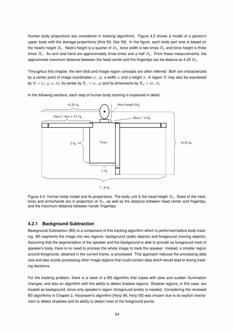
Human body proportions are considered in tracking algorithms. Figure 4.2 shows a model of a person’s
upper body with the average proportions [Arts 09, Dist 09]. In the figure, each body part size is based on
the head’s height Hh. Neck’s height is a quarter of Hh, torso width is two times Hh and torso height is three
times Hh. An arm and hand are approximately three times and a half Hh. From these measurements, the
approximate maximum distance between the head center and the fingertips can be deduce as 4.25 Hh.
Throughout this chapter, the skin blob and image region concepts are often referred. Both are characterized
by a center point of image coordinates (x, y), a width w and a height h. A region R may also be expressed
by R = (x, y, w, h), its center by Rc = (x, y) and its dimensions by Rd = (w, h).
In the following sections, each step of human body tracking is explained in detail.
Figure 4.2: Human body model and its proportions. The body unit is the head heigth Hh. Sizes of the neck,torso and arms/hands are in proportion of Hh, as well as the distance between head center and fingertips,and the maximum distance between hands’ fingertips.
4.2.1 Background SubtractionBackground Subtraction (BS) is a component of this tracking algorithm which is performed before body track-
ing. BS segments the image into two regions: background (static objects) and foreground (moving objects).
Assuming that the segmentation of the speaker and the background is able to provide as foreground most of
speaker’s body, there is no need to process the whole image to track the speaker. Instead, a smaller region
around foreground, obtained in the current frame, is processed. This approach reduces the processing data
size and also avoids processing other image regions that could contain data which would lead to wrong track-
ing decisions.
For the tracking problem, there is a need of a BS algorithm that copes with slow and sudden illumination
changes, and also an algorithm with the ability to detect shadow regions. Shadow regions, in this case, are
treated as background, since only speaker’s region (foreground pixels) is needed. Considering the reviewed
BS algorithms in Chapter 2, Horprasert’s algorithm [Horp 99, Horp 00] was chosen due to its explicit mecha-
nism to detect shadows and its ability to detect most of the foreground points.
24

The implemented BS algorithm includes all the speed-up techniques presented in [Horp 99], except paral-
lel processing because the processing of a single image region makes the algorithm simpler. Moreover, there
were not found significant time improvements when using a global standard deviation for all the pixels (Global
S in [Horp 99]), compared to local si. Furthermore, it yielded more wrongly classified foreground pixels. As a
consequence, local si was used instead of a global S.
In this algorithm, it is assumed that there is a period of time T to compute the background model, before
the speaker becomes visible in the camera’s field of view. It is also assumed that there are slight movements
in the audience in the same period of time.
Let I(t) be the processed image at time t, with width W and height H . I(x,y,t) denotes the RGB pixel
in coordinates (x,y), where x and y are the image columns and rows, respectively. Let also IB(t) be the
binary image with the same dimensions of I(t). The coordinate system of I(t) is shown in Figure 4.3.
Figure 4.3: Image coordinates system. x and y represent the image columns and rows, respectively.
Some features have been improved or changed from the original algorithm, namely an adaptive updating
of the background model, a technique to reduce the number of processed pixels and the pixel classification
was simplified into two categories. These changes from the original algorithm are now described in detail.
Background Model UpdateThis algorithm has been improved to adaptively update the background model as the room illumination
changes over the presentation time. The background model B(t) is updated for every time t and pixel of
coordinates (x,y) and is given by:
B(x, y, t) = (1− αB) B(x, y, t− 1) + αB I(x, y, t) (4.1)
where αB is the update rate. This update is only performed for pixels classified as background in t − 1,
otherwise foreground pixels would be gradually incorporated in background. In order to renew B every 10
minutes, αB is computed from (4.1) by setting I(x, y, t) = 0 and assuming that the current model B(t) forgets
95% of the its initial value B(0). αB is given by:
αB = 1−(B(t)B(0)
) 1t
(4.2)
where B(t)B(0) = 0.05 and t = 15000 is the corresponding number of frames of a 10 minutes video at 25 fps.
This leads to αB = 0.000199696.
Reduction of the processing image regionSince speaker occupies a small region of the image, it is not needed to perform BS to the whole image, but
inside the region around the speaker. As a result, BS is computed faster because there are less pixels to
25
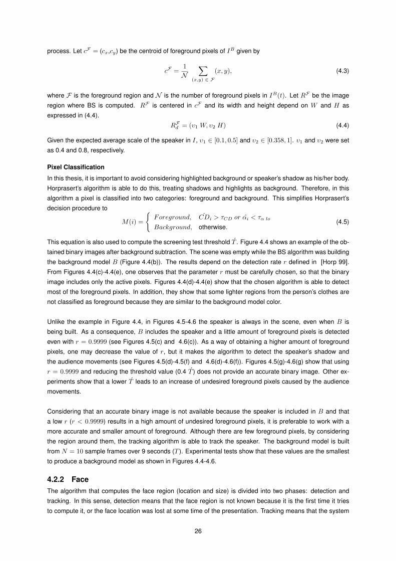
process. Let cF = (cx,cy) be the centroid of foreground pixels of IB given by
cF =1N
∑(x,y) ∈ F
(x, y), (4.3)
where F is the foreground region and N is the number of foreground pixels in IB(t). Let RF be the image
region where BS is computed. RF is centered in cF and its width and height depend on W and H as
expressed in (4.4).
RFd = (υ1 W,υ2 H) (4.4)
Given the expected average scale of the speaker in I, υ1 ∈ [0.1, 0.5] and υ2 ∈ [0.358, 1]. υ1 and υ2 were set
as 0.4 and 0.8, respectively.
Pixel Classification
In this thesis, it is important to avoid considering highlighted background or speaker’s shadow as his/her body.
Horprasert’s algorithm is able to do this, treating shadows and highlights as background. Therefore, in this
algorithm a pixel is classified into two categories: foreground and background. This simplifies Horprasert’s
decision procedure to
M(i) =
Foreground, CDi > τCD or αi < τα lo
Background, otherwise.(4.5)
This equation is also used to compute the screening test threshold T . Figure 4.4 shows an example of the ob-
tained binary images after background subtraction. The scene was empty while the BS algorithm was building
the background model B (Figure 4.4(b)). The results depend on the detection rate r defined in [Horp 99].
From Figures 4.4(c)-4.4(e), one observes that the parameter r must be carefully chosen, so that the binary
image includes only the active pixels. Figures 4.4(d)-4.4(e) show that the chosen algorithm is able to detect
most of the foreground pixels. In addition, they show that some lighter regions from the person’s clothes are
not classified as foreground because they are similar to the background model color.
Unlike the example in Figure 4.4, in Figures 4.5-4.6 the speaker is always in the scene, even when B is
being built. As a consequence, B includes the speaker and a little amount of foreground pixels is detected
even with r = 0.9999 (see Figures 4.5(c) and 4.6(c)). As a way of obtaining a higher amount of foreground
pixels, one may decrease the value of r, but it makes the algorithm to detect the speaker’s shadow and
the audience movements (see Figures 4.5(d)-4.5(f) and 4.6(d)-4.6(f)). Figures 4.5(g)-4.6(g) show that using
r = 0.9999 and reducing the threshold value (0.4 T ) does not provide an accurate binary image. Other ex-
periments show that a lower T leads to an increase of undesired foreground pixels caused by the audience
movements.
Considering that an accurate binary image is not available because the speaker is included in B and that
a low r (r < 0.9999) results in a high amount of undesired foreground pixels, it is preferable to work with a
more accurate and smaller amount of foreground. Although there are few foreground pixels, by considering
the region around them, the tracking algorithm is able to track the speaker. The background model is built
from N = 10 sample frames over 9 seconds (T ). Experimental tests show that these values are the smallest
to produce a background model as shown in Figures 4.4-4.6.
4.2.2 FaceThe algorithm that computes the face region (location and size) is divided into two phases: detection and
tracking. In this sense, detection means that the face region is not known because it is the first time it tries
to compute it, or the face location was lost at some time of the presentation. Tracking means that the system
26

(a) Original image (b) Background model (c) Binary image with r = 0.9999
(d) Binary image with r = 0.999999 (e) Binary image with r = 0.99999999
Figure 4.4: Example of the binary images using different values of r. In this example, the scene is emptywhile the background model is being built.
knows the face region at time t − 1 and is trying to compute it for time t. Face region at time t is denoted by
the rectangular region F (t) = (x,y), with width w and height h, where (x,y) are the coordinates of the center
point of F (t). Both phases are described below, as well as the algorithm to compute the skin blobs.
Face Detection
Face detection is accomplished through skin blobs. Skin blobs are rectangular regions computed from I and
are characterized by their center (x,y) which matches with coordinates of I, and by their width w and height
h. In general, a skin blob is an image region where there is an 8-connected component of pixels classified as
skin colors. Skin blobs algorithm is later described.
Assuming that the speaker is standing and there is no other person in the image faced to the camera, the face
is the highest skin blob of I (blob with the smallest y). In order to search for the face only where is movement,
region RF is used. Limiting the search of the face to RF avoids the detection of skin blobs that cannot be the
face and also reduces the number of pixels to process. Once RF is set, a list of skin blobs Q is computed.
Q contains only blobs whose skin points number is between β1 and β2. For face detection β1 = 9 because it
is the minimum acceptable value which a face shows in a frontal view, given the distance between the face
and the camera, and the image resolution used (W × H). A lower β1 would reduce the face detection rate
because the number of blobs increases and most of them would be the hands or some skin-colored object
within the classroom. By measuring the speaker face scales from the farthest and closest locations to the
camera, one can obtain an increase by a factor of three. Therefore, by setting β2 = 3 β1 = 27, very large
blobs are ignored. In addition, it is important that the detected face region in this phase is a model of the
face dimensions, because it is posteriorly used to improve face and hand tracking. Note that β2 is set only
once, whereas β1 is updated in (4.17) for every t. m =∞ is set in a way that S returns all the computed blobs.
27

(a) Original image (b) Background model (c) Binary image with r = 0.9999
(d) Binary image with r = 0.95 (e) Binary image with r = 0.90 (f) Binary image with r = 0.85
(g) Binary image with r = 0.9999 and0.4T
Figure 4.5: Example of the binary images using different values of r. In this example, the speaker is alreadyvisible in the image while the background model is being built.
Although it seems to be reasonable to choose now the highest blob as the face region, an additional op-
eration is needed. Before assigning a blob to the face, some restrictions to the blobs’ ratios must be applied,
in order to avoid choosing as face a region which contradicts the human proportions. Obviously, face width
cannot be too large compared to its height and vice-versa. In addition, the illumination within the room could
cause some skin-like regions, besides the real face. So, from Q, only the blobs that satisfy the following
conditions are considered:QiwQih
< r (4.6)
andQihQiw
< r (4.7)
where Qi is the i-th blob of Q (i ∈ 0, · · · ,#(Q)− 1 and #(Q) is the cardinality of Q), Qiw is the blob width,
Qih is the blob height and r is the maximum dimension ratio. According to [Arts 09, Dist 09], head width Hw
28
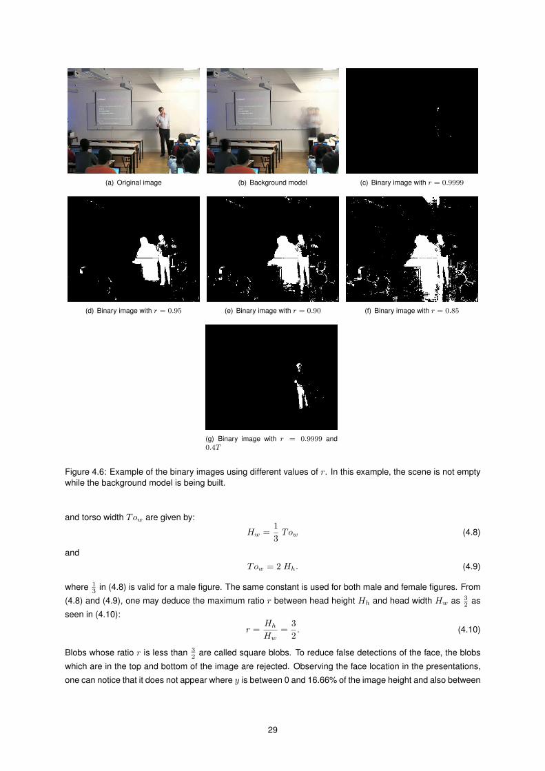
(a) Original image (b) Background model (c) Binary image with r = 0.9999
(d) Binary image with r = 0.95 (e) Binary image with r = 0.90 (f) Binary image with r = 0.85
(g) Binary image with r = 0.9999 and0.4T
Figure 4.6: Example of the binary images using different values of r. In this example, the scene is not emptywhile the background model is being built.
and torso width Tow are given by:
Hw =13Tow (4.8)
and
Tow = 2 Hh. (4.9)
where 13 in (4.8) is valid for a male figure. The same constant is used for both male and female figures. From
(4.8) and (4.9), one may deduce the maximum ratio r between head height Hh and head width Hw as 32 as
seen in (4.10):
r =Hh
Hw=
32. (4.10)
Blobs whose ratio r is less than 32 are called square blobs. To reduce false detections of the face, the blobs
which are in the top and bottom of the image are rejected. Observing the face location in the presentations,
one can notice that it does not appear where y is between 0 and 16.66% of the image height and also between
29
69.44 and 100%. Finally, face region is set as:
F (t) = q (4.11)
where q = Qi, i = arg mink
Qky and Qky is the y coordinate of the blob. Figure 4.7(a) shows an example of
a presentation image where the face is visible and Figure 4.7(b) corresponds to region RF . The blob list Q
obtained from RF are shown in Figure 4.7(c), but some of them are rejected because they fail conditions (4.6)
and (4.7). In this example, the final blobs are shown in Figure 4.7(d) and the highest is associated to the face.
As may be observed from the face tracking algorithm description, this algorithm is able to adapt the face
(a) Original image (b) Foreground region of4.7(a)
(c) All the skin blobs of theforeground region
(d) Square skin blobs
Figure 4.7: Example of face detection with skin blobs.
scale over the time. This capability also brings the difficulty of limiting the face dimensions. Without a mech-
anism to limit the face dimensions, F (t) could be associated to a very large skin blob which could not be the
speaker’s face. This mechanism was particularly added to cope with situations where the hands are so close
to the face that they belong to the same blob. In these situations, the algorithm must be able to let F (t) di-
mensions increase because the blob includes the face and a hand, but it must also limit its dimensions so they
never exceed some predefined values. This mechanism is now described. Let F d be a region representing
the default face. F d is a region whose location and dimensions are used as models to distinguish between
skin blobs which could or not be the face. Additionally, default face provides the average face dimensions
30

which are used to compute torso and hand regions. F d is defined as:
F d = (qx, qy, dγ1 qwe, dγ1 qhe) (4.12)
where γ1 is set to 1.1, in order to slightly increase the default face, compared to q. This increase is reason-
able because it is unlikely that q corresponds to a face frontal view, which would result in a bigger blob. The
operator d e denotes the ceil function. Let F l = (γ2 Fdw, γ2 F
dh ) be the limit of the face dimensions (width and
height), where γ2 ∈ [1, 1.5]. Dimensions of F d are used to compute face and torso regions, so γ2 cannot be
to big to avoid large errors when tracking them. When Fw(t) and Fh(t) overcome F l, they are replaced by
F dw and F dh , respectively. This is a simple method controlled by γ1 and γ2.
At the end of face detection phase, the real face blob is stored as F r(t) = q denoting the region where
the face was found without any dimension changes, unlike F (t) and F d. F r(t) is a region which could con-
tain part of the speaker’s neck and is used in the hand tracking algorithm to define the search region of the
hands.
Face Tracking
In the previous phase, face location F (t − 1) was unknown, so a large region of I had to be processed until
some skin blob was found. In this phase, only a very small region is processed because it is assumed that
the speaker does not move rapidly, therefore F (t) is in the neighborhood of F (t− 1). Thus, the approach for
tracking the face is look for the skin blobs in the neighborhood of F (t− 1), and assign to F (t) the blob whose
similarity with F (t− 1) is the highest.
Firstly, the algorithm sets the image region RF where the face is expected to be. Center of RF is the same
of F (t− 1) and its dimensions are defined in (4.13) and (4.14).
RFw = Fw(t− 1) + 2 δF 1 (4.13)
RFh = Fh(t− 1) + 2 δF 2 (4.14)
δF 1 and δF 2 are the offsets of F (t − 1) that introduce points from its neighborhood and they are given by
(4.15) and (4.16).
δF 1 = dβ3Fw(t− 1)e (4.15)
δF 2 = dβ4Fh(t− 1)e (4.16)
The operator ceil is used rather than the floor to ensure that the offsets are always greater than zero. Using the
floor function, offsets could become zero and RF would not be big enough to include the probable location
of the face. Constants β3 and β4 control the amount of the offsets in coordinates x and y, respectively;
consequently the number of pixels to process increases. From t− 1 to t, it is expected that the speaker’s face
moves more significantly in x coordinate than in y. In addition, sudden movements from consecutive frames
are also not expected. As a result, β3 is greater than β4 because the offset in x is more relevant to keep
tracking face’s blob. On the other hand, to reduce the number of processed pixels, β3 and β4 are kept small,
belonging to the interval ]0, 1[. After setting RF , the blob list Q is computed. In the tracking phase, β1 is
based on the area of F (t− 1) as a way of adapting to the face dimensions, and also reducing the number of
undesired blobs. This strategy considers that face dimensions do not change abruptly from time t− 1 to t. β1
is computed as:
β1 = d β5 Fw(t− 1) Fh(t− 1) e (4.17)
31

β5 was tested for interval [0.05, 0.5] for a video sequence of 1623 frames. Figure 4.8 shows the number of
detection phases for each value of β5, where the correct value is 1. By the results, one can conclude that the
best values of β5 are within the interval ]0, 0.06] and the optimal value is 0.06.
Once Q has been obtained, all of its blobs are checked about their dimensions. As mentioned before, the
Figure 4.8: Number of tracker initializations (or face detection phases) for each β5 value. Horizontal axisrepresents the value of β5. Vertical axis shows the corresponding number of detection phases.
face and a hand (or even the two hands) when close enough in the image, can belong to the same skin blob.
Besides, when the background is close to the face, it can be included in the same skin blob of the face, if the
background is considered to have skin colors. As a result of these two situations, this blob candidate to face
region is too large to be a face and is rejected. The way this rejection is handled is simple. If there is at least
one blob q ∈ Q that intersects F (t−1) and overcomes F l, then all the blobs are rejected and F (t) is set with
F (t− 1). This approach avoids large face regions, although it could lose some precision in the face location
while other objects are merged with the face.
Sometimes a hand can be tracked as if it was the face. It can happen when the face and a hand are in
the same skin blob, the speaker lowers his/her hand and the function Ψ decides that this blob is the most
similar to the previous face. In this situation, the face can be correctly tracked again in two cases: 1) the hand
comes back to where the face is and now Ψ has better blobs to compare with, or 2) the speaker’s hand is lost
(the supposed face) and the algorithm goes to the detection phase. Knowing this problem and its causes, it
is still not easy to solve it completely. However, there is a way of reducing the time that the hand is wrongly
tracked, instead of the face. The solution is, as mentioned before, to assume that the speaker’s face is the
highest skin blob within RF . Therefore, every time the face is being tracked through the above algorithm,
providing Q, face detection algorithm looks for a face candidate above the highest blob of Q. When a face
candidate which does not intersect hand regions at time t − 1 is found, it is assigned to the face region re-
placing the previous region.
For the case that no face candidate is found, there is a procedure to associate a blob with the face region.
The assignment is shown in (4.18).
F (t) =
unknown if #(Q) = 0Q0 if #(Q) = 1Ψ(F (t− 1), Q) otherwise.
(4.18)
32

In (4.18), Ψ returns a blob q ∈ Q which presents the highest similarity with the previous face region. Ψ is
expressed by:
Ψ(b,Q) = Qi, i = arg mink
S(b,Qk) (4.19)
where b is the reference region to compare with the blob list. S is expressed by:
S(b1, b2) = w1 |a(b1)− a(b2)|+
w2 ||c(b1)− c(b2)||2 (4.20)
where b1 and b2 are two blobs, operator a provides the pixels number of a blob, operator c gives the centroid
of a region, w1 = 0.5 and w2 = 1 - w1 are the weights given to each part of the equation. A high w1 would
cause the algorithm to choose blobs with a similar area, but that could be far from the reference region; a high
w2 would tend to choose the closest blob with little account about the previous size of the region. This way,
both parameters are equally balanced.
Skin Blobs
Skin blob computation is an essential operation in the developed tracking algorithm. It is used both in face
tracking and hand tracking. To complete all the algorithms used in this section, the skin blobs algorithm is now
described.
The main idea of the skin blobs algorithm is to classify each pixel as being skin-like or not, label the con-
nected skin pixels with the same identifier and compute the bounding boxes of pixels with the same identifier
(label). Let R be a region of I centered in (Rx, Ry), M be a binary skin map of width Rw and height Rh. To
obtain the skin pixels within R, M(x′′, y′′) is computed for each (x′, y′) ∈ S as:
M(x′′, y′′) = Skin( I(x′, y′) ) (4.21)
where
(x′′, y′′) = (x′ −Rx +Rw2, y′ −Ry +
Rh2
). (4.22)
Skin was expressed in (2.5), and S is defined by
S = Rx −Rw2, Rx −
Rw2
+ 1, · · · , Rx +Rw2 × Ry −
Rh2, Ry −
Rh2
+ 1, · · · , Ry +Rh2 (4.23)
where × denotes the Cartesian product of two sets. The skin detection method used was chosen due to its
simplicity, speed, satisfactory detection rate for the described scene conditions, and because no color space
conversion was needed. Experimental tests show that the classifier defined in (2.5) detects less false positives
than the classifier expressed by (2.7). After obtainingM , a map of skin labels L is computed, where L(x′′, y′′)stores the label of pixel in coordinates (x′′, y′′). M and L have the same dimensions. In Figure 4.9 is shown
an example of the map M (Figure 4.9(a)) and its corresponding map L (Figure 4.9(b)). L is initialized as:
L(x′′, y′′) = 0, ∀ (x′′, y′′) ∈ L (4.24)
and for each 8-connected component of M , a different label is assigned. Then, the bounding box of each
labeled component is computed, but only for those components which have at least β1 skin points. At the
end, each blob q coordinates are converted to (x, y), becoming the new blob q′
as
q′
c = qc +Rc. (4.25)
33

(a) Binary map of skin (b) Map of skin labels
Figure 4.9: Example of a binary skin map and its corresponding labels.
This algorithm also includes a parameter m which denotes the maximum returned blobs. When there are
more than m blobs, the returned blobs are the m biggest blobs, where the size is computed as the bounding
box area.
4.2.3 TorsoTorso region To(t) is detected in every image I and requires that face region is known. Its detection is based
on two information sources: torso’s edge points and knowledge about the human proportions. Firstly, the
detection method defines a region RTo where the torso is expected to be, depending on the face location
and scale. The expected location of To(t) is below the face, since it is assumed the speaker is standing and
upright. Secondly, edge points within RTo are computed from I as shown in Figure 4.10(a). Then, RTo is
split into regions RTo1 and RTo2 (Figure 4.10(b)). Regions RTo1 and RTo2 are considered to contain right and
left boundaries of the torso, respectively. Then, the approximate right and left boundaries are the median of
x coordinate in the corresponding regions. Once obtained right and left boundaries, the remaining top and
bottom are computed from the knowledge of human proportions (Figure 4.10(c)). The details of the method
are given below.
Torso is expected to be within region RTo, whose center RToc and dimensions RTod are expressed as:
RToc = ( Fx(t), Fy(t)− Fh(t)2
+RToh
2) (4.26)
and
RTod = ( (φ1 + φ2) ω, φ3 ω) (4.27)
where ω = Hh. Assuming that
F dh = Nh +Hh (4.28)
and observing that
Nh =14Hh (4.29)
from Figure 4.2, Hh is deduced as:
Hh =45F dh (4.30)
whereNh is the neck’s height. Although torso region is below Fy(t), the top ofRTo and F (t) is the same. If the
top of RTo was set to somewhere below Fy(t), when a hand/arm and face were in the same blob, the bottom
of F (t) could already include the torso. As a consequence, the region detected as torso, would return mostly
waist and legs. So, face region top is used to avoid this situation. As a result of the human body proportions,
φ1 = 2 is associated to the torso expected proportion (2 faces height) and φ2 = 2 adds some tolerance to RTow .
34
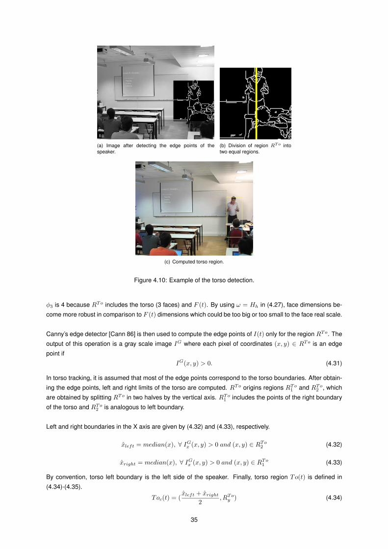
(a) Image after detecting the edge points of thespeaker.
(b) Division of region RTo intotwo equal regions.
(c) Computed torso region.
Figure 4.10: Example of the torso detection.
φ3 is 4 because RTo includes the torso (3 faces) and F (t). By using ω = Hh in (4.27), face dimensions be-
come more robust in comparison to F (t) dimensions which could be too big or too small to the face real scale.
Canny’s edge detector [Cann 86] is then used to compute the edge points of I(t) only for the region RTo. The
output of this operation is a gray scale image IG where each pixel of coordinates (x, y) ∈ RTo is an edge
point if
IG(x, y) > 0. (4.31)
In torso tracking, it is assumed that most of the edge points correspond to the torso boundaries. After obtain-
ing the edge points, left and right limits of the torso are computed. RTo origins regions RTo1 and RTo2 , which
are obtained by splitting RTo in two halves by the vertical axis. RTo1 includes the points of the right boundary
of the torso and RTo2 is analogous to left boundary.
Left and right boundaries in the X axis are given by (4.32) and (4.33), respectively.
xleft = median(x), ∀ IGx (x, y) > 0 and (x, y) ∈ RTo2 (4.32)
xright = median(x), ∀ IGx (x, y) > 0 and (x, y) ∈ RTo1 (4.33)
By convention, torso left boundary is the left side of the speaker. Finally, torso region To(t) is defined in
(4.34)-(4.35).
Toc(t) = (xleft + xright
2, RToy ) (4.34)
35

Tod = ( xleft − xright + 1, RToh ) (4.35)
One can perceive that face region is also included in To(t). This decision was made due to the uncertainty
about the location of the face bottom when the hands are merged to the face blob. Since the torso location
is needed for activity recognition and precision is required, this approach provides less variations in torso
centroid, if compared to an approach which considers only the region below Fy(t).
4.2.4 HandsHand tracking is performed through skin blobs, after knowing F (t). Since hands cannot be too far from the
face, face position and dimensions are used to define a search region for the hands. In this problem, it was
assumed that hands could be seen in several locations. Hands may be over the torso plane, over the legs
plane, and at each side of the head and torso. The technique to discover hand’s positions and dimensions
has two phases: detection and tracking.
Detection phase has four steps and it is performed when both hands’ location is unknown. The first step
consists in defining three search regions where hands are expected to be visible. The second step is to com-
pute all the existing skin blobs within the search regions. The third step is to reject skin blobs which cannot be
hands because they are too large or too far or close from the head, among other rejection rules. Fourth step
is associating a given blob to a hand.
Tracking phase is started when the previous hand region is known. It has some similar steps with detec-
tion phase, such as computing skin blobs, their filtering and association. The algorithm is described below in
more detail. This phase also includes some detection steps which are performed when one of the hands is
unknown.
Detection phase
Let LH(t) and RH(t) be the regions of left and right hands at time t. Hands can visible in several locations,
therefore three searching regions are defined. Let RHa1 and RHa3 be the regions on the right and left sides
of F (t), respectively. Let also RHa2 be a region below the F (t) which intersects To(t). Figure 4.11(a) shows
how these regions are placed relatively to speaker’s body. RHa1 and RHa3 are on the left and right sides of
speaker’s face (from reader’s view), respectively. RHa2 is below speaker’s face. Face region is highlighted with
a red rectangle. Figure 4.11(b) shows the pixels classified as skin painted in orange. From Figure 4.11(b),
one can observe the existence of many skin blobs within the three regions. The algorithm chooses at most 2
skin blobs and rejects the others. RHa1 is given by:
RHa1c = (Fx(t)− (δHa + ε), Fy(t)− Fh(t) ) (4.36)
and
RHa1d = ( δHa, ψ4 ω ) (4.37)
where
δHa = d(1 + ψ3) Fw(t)e. (4.38)
Equation (4.38) forces RHa1 to move at least one face width to the right side and ψ3 ∈ [0, 3.5] controls the
region’s width. Its interval is based on body proportions mentioned above. ψ4 ∈ [2, 3.5] in order to include
from the head side to some of the torso. In Figure 4.11(a), ψ3 = 0 and ψ4 = 3.5. RHa1 and RHa3 are
symmetrical in the vertical axis of the face. As a consequence, only RHa3x is changed to
RHa3x = Fx(t) + δHa + ε. (4.39)
36

(a) Image regions where the hands are searched. (b) Image with hand search regions and skin pixels(orange pixels).
Figure 4.11: Regions around the speaker where hand blobs are searched.
RHa1 and RHa3 cannot intersect with F (t) because otherwise skin blobs of RHa1 and RHa3 could join the face
blob, if these regions were adjacent. So an offset ε is required. The condition which avoids this adjacency is:
ζ1 − ζ2 ≥ 2 (4.40)
where ζ1 = RHa3x −RHa
3w
2 is the left boundary of RHa3 , and ζ2 = Fx + Fw
2 is the right boundary of region F (t).The reasoning is analogous for RHa1x . From condition 4.40, ε is given by:
ε ≥ 2− 12
(d(1 + ψ3)Fwe − Fw
)(4.41)
and ε ≥ 2, if ψ3 = 0.
Moreover, RHa2 is expressed by:
RHa2c = (F rx (t), F ry (t) + F rh(t) ), (4.42)
and
RHa2d = ( ψ1 ω, ψ2 ω ) (4.43)
where RHa2c is the center point of RHa2 , ψ1 = 8 because the maximum distance between hands is eight times
the head height; ψ2 = 3.5 because 3.5 ω is the maximum length of an arm and hand. F r(t) may include
speaker’s neck, so to avoid detecting neck’s and head’s skin blobs, F rh(t) is added to the y component. In
(4.43) ω is used because it provides a better approximation to head’s height, hence a better approximation of
the region where the hands can be visible.
Once defined the search regions, the skin blobs algorithm computes at most two blobs (m = 2). Let Q
be the obtained blob list. In this process, if the same blob is included more than once in some of these re-
gions, only one is considered. Blobs of Q are then filtered in order to remove those which cannot be accepted
as hands. This filter includes a set of rules that blobs cannot break. If they do, they are removed from Q.
There are six rules:
1. Blob’s area must be greater than 1.
2. Distance between Fc and the blob farther boundary in x coordinate must be less than 4.25 ω due to
human body part sizes (see Figure 4.2).
37

3. Distance between Fc and the blob farther boundary in y coordinate must be less than 4.25 ω due to
human body part sizes (see Figure 4.2).
4. Blob cannot intersect Fc(t).
5. Blob width must be less than 2 ω.
6. Blob’s area must be smaller than the double of face’s area.Rule 1 rejects blobs whose size is so small that they could not be considered as hands. Rule 2 and 3 use
the knowledge about the maximum distances between face and the fingertips to reject blobs. Rule 4 rejects
blobs close to the face, considering they may be part of the face or neck. Rule 5 tolerates blobs whose width
is less than 2 ω because when the arms without clothes and hands are together over the torso, they are
approximately (at most) the torso width (2 ω). Rule 6 limits the hand size by rejecting too large blobs and
gives a tolerance of 2 faces in order to track an unclothed arm or both arms together; it is still preferable than
no tracking at all.
After filtering Q, its blobs are assigned to LH(t) and RH(t). If there is only one blob in Q, the blob is
assigned to the left hand and the default hand Had(t) = Q(0). Had is used as a hand model in the tracking
phase in (4.19). When Q contains two blobs, the assignment is as follows:
LH(t) = Qi (4.44)
and
RH(t) = Qj (4.45)
where i = arg maxk
Qkx and j = arg mink
Qkx. Had is now a combination of both hands dimensions as a way
of storing a mixture of both. The center of Had is LHc(t) and its dimensions are the averages of the two
hands dimensions.
Tracking phase
Hand tracking phase is started when at least one of the hands’ location is known. Left and right hands are
tracked by this order, although the algorithm is very similar. The algorithm starts by defining a search region
RHa for the hand Ha (left or right). From time t − 1 to t it is expected that the hand is in the neighborhood
of the previous location. Therefore, region RHa is centered in the previous hand location Ha(t − 1) and
its dimensions are increased as a way of including previous location and also its involving neighborhood.
Therefore, dimensions of RF are:
RFw = Haw(t) + d ψ5 Haw(t) e (4.46)
and
RFh = Hah(t) + d ψ5 Hah(t) e (4.47)
where ψ5 controls the amount of the hand’s neighborhood which is evaluated. A high ψ5 provides more
robustness to fast movements, but also requires more pixel processing. Good tracking results for slow and
fast movements can be obtained for the interval [0.4, 1.8]. After defining RHa, a blob list Q is obtained and
its blobs are filtered as previously mentioned. Before assigning a blob to Ha, those blobs which intersect LH
are removed from Q, if Ha corresponds to the right hand. This is done to avoid assigning a hand’s blob to the
other hand. Hereafter, the assignment decision is made with the following rules:
Ha(t) =
unknown if #(Q) = 0Q0 if #(Q) = 1Ψ(Had(t), Q) otherwise.
(4.48)
38

When one of the hands is unknown, the procedure is similar to the detection phase. It searches for skin blobs
in regions RHa1 , RHa2 and RHa3 , filters the blobs, removes some blob already associated to the left hand, if
detecting the right hand; and associates one blob to the hand. This association depends on the cardinality of
Q. When there is only one blob and the algorithm is trying to detect left hand, that blob is associated to left
hand. But if the blob is very close to the previous right hand, then it is considered to be the right hand. On
the contrary, when detecting the right hand and the left is far, the blob is assigned to the right hand. The other
association decisions are described by (4.49).
Ha(t) =
unknown if #(Q) = 0Qi, i = arg max
k
Qkx if #(Q) = 2 and Ha is left hand
Qi, i = arg mink
Qkx if #(Q) = 2 and Ha is right hand
Ψ(Had(t), Q) if #(Q) ≥ 3.
(4.49)
This set of steps is performed for left hand first. Then, they are repeated for the other hand. However, as
described before, a blob can be associated to the right hand when the algorithm is trying to detect/track the
left hand. In that case, the above steps are no longer needed for time t. At the end of tracking phase, if the
assigned blobs to the hands break the convention that LHx > RHx, those blobs are swapped. Besides,
when LHx(t) < Fx(t) and the right hand is unknown, the blob assigned to LHx is considered to be the right
hand, and the left hand is set to unknown. Similarly, when RHx(t) > Fx(t), the blob of RHx(t) is considered
the left hand, and right hand is set to unknown.
After the detection and tracking phases, Had is updated using LH and RH sizes, in order to provide the
best hand model. Sizes of Had are updated using both hands sizes. Default hand width is given by:
Hadw(t+ 1) = θ Hadw(t) + (1− θ) LHw(t) +RHw(t)2
(4.50)
and its height is
Hadh(t+ 1) = θ Hadh(t) + (1− θ) LHh(t) +RHh(t)2
(4.51)
where θ = 0.5 rapidly updates Had(t + 1). When only one of the hands location is known, default hand is
updated with the known hand data.
4.3 Recognizing ActivitiesIn an interactive presentation, the speaker can simultaneously perform several activities. As a consequence,
it is not possible to recognize all the activities with a single classifier, since it would only be able to recognize
one activity at each time. Therefore, the system requires a separate classifier for each activity. Each classifier
is binary, since it reports if the activity was detected or not detected. In the system, each activity classifier
is trained with positive and negative examples of the activity using a classification algorithm. Each trained
classifier is then able to detect a specific type of activity.
The activity recognition process includes the following steps:
1. Describe the activity’s characteristics.
2. Collect training and test samples of the activity (training and test video set).
3. Label each occurrence of the activity as a positive or negative example of the activity for the video set.
4. Select the classification algorithm used to train and test the activity.
39

5. Train and test the activity with the collected examples.
Next sections detail the characterization of activities, the classification algorithms and the training and test
steps.
4.3.1 Characterizing ActivitiesEach activity is characterized by the features involved, sliding window and method of construction of the fea-
ture vector. Sliding window indicates the number of frames used to detect an activity. Features considered
in this thesis are related to speaker’s body points, such as position, speed, distance between points, among
others.
Hereafter, a characterization of the activities is provided, more specifically their description, motivation, main
features, sliding window sizes and methods to create the feature vector.
Activity Description and Features
This section describes every activity and corresponding motivation and features. Table A.1 lists the features
used in the feature sets of each activity and how they were computed.
Activity A (“Speaker has bent”) is considered to have occurred when the speaker bends his/her back and
his/her head becomes lower. The developed tracker provides face and torso location, but not if the torso has
bent. Therefore, activity A happens when speaker’s face becomes lower in a short period (see two exam-
ples of activity A in Figure 4.12). The motivation for recognizing activity A is to detect that the speaker has
changed the current slide by only focusing on speaker’s movements. In Figures 4.12(d)- 4.12(f), one observes
the speaker bending to change the slide in his computer. According to the description, reasonable features
to use are the face and torso displacements over the time in y because there should occur an increasing dis-
placement of these body parts, and also the face area since it often decreases as the speaker bends. Three
feature sets combining the previous features are listed in Table 4.1.
Table 4.1: Feature set of activity A.
Set Featuresname
A1 F vy (t), Tov
y(t), [Fy(t)− Fy(t− u)], pixels(F (t))A2 F v
y (t), Tovy(t), pixels(F (t))
A3 A1 and [Fy(t)− Fy(t− v)] (u 6= v)
Activity B (“Speaker’s face is visible”) occurs when the speaker’s face is visible in the image (Figure 4.13). In
this activity, both frontal and side views are accepted. Recognizing B is motivated by knowing how much time
the speaker is facing the audience during a presentation, and how often he/she is not facing the audience.
Features for B are the face location (in x and/or y) because these provide information about whether the face
is visible or not (see Table 4.2).
Table 4.2: Feature set of activity B.
Set Featuresname
B1 Fx(t)
B2 Fy(t)
B3 B1 and B2
40
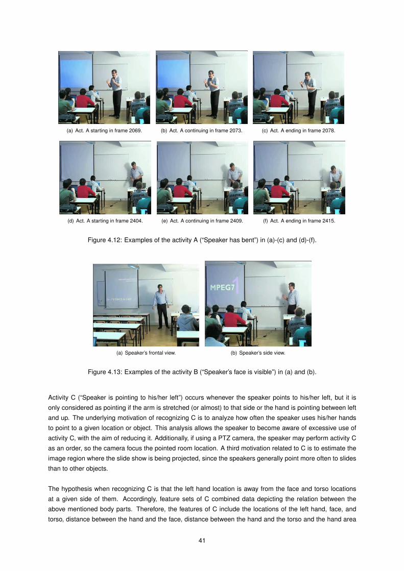
(a) Act. A starting in frame 2069. (b) Act. A continuing in frame 2073. (c) Act. A ending in frame 2078.
(d) Act. A starting in frame 2404. (e) Act. A continuing in frame 2409. (f) Act. A ending in frame 2415.
Figure 4.12: Examples of the activity A (“Speaker has bent”) in (a)-(c) and (d)-(f).
(a) Speaker’s frontal view. (b) Speaker’s side view.
Figure 4.13: Examples of the activity B (“Speaker’s face is visible”) in (a) and (b).
Activity C (“Speaker is pointing to his/her left”) occurs whenever the speaker points to his/her left, but it is
only considered as pointing if the arm is stretched (or almost) to that side or the hand is pointing between left
and up. The underlying motivation of recognizing C is to analyze how often the speaker uses his/her hands
to point to a given location or object. This analysis allows the speaker to become aware of excessive use of
activity C, with the aim of reducing it. Additionally, if using a PTZ camera, the speaker may perform activity C
as an order, so the camera focus the pointed room location. A third motivation related to C is to estimate the
image region where the slide show is being projected, since the speakers generally point more often to slides
than to other objects.
The hypothesis when recognizing C is that the left hand location is away from the face and torso locations
at a given side of them. Accordingly, feature sets of C combined data depicting the relation between the
above mentioned body parts. Therefore, the features of C include the locations of the left hand, face, and
torso, distance between the hand and the face, distance between the hand and the torso and the hand area
41
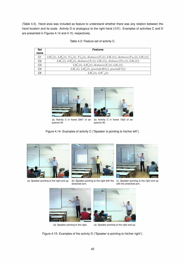
(Table 4.3). Hand area was included as feature to understand whether there was any relation between the
hand location and its scale. Activity D is analogous to the right hand (RH). Examples of activities C and D
are presented in Figures 4.14 and 4.15, respectively.
Table 4.3: Feature set of activity C.
Set Featuresname
C1 LH′x(t), LH
′y(t), To
′x(t), To
′y(t), distance(Fc(t), LHc(t)), distance(Toc(t), LHc(t))
C2 LH′x(t), LH
′y(t), distance(Fc(t), LHc(t)), distance(Toc(t), LHc(t))
C3 LH′x(t), LH
′y(t), distance(Fc(t), LHc(t))
C4 LH′x(t), LH
′y(t), pixels(LH(t)), pixels(F (t))
C5 LH′x(t), LH
′y(t)
(a) Activity C in frame 2847 of se-quence 34.
(b) Activity C in frame 1022 of se-quence 39.
Figure 4.14: Examples of activity C (“Speaker is pointing to his/her left”).
(a) Speaker pointing to the right and up. (b) Speaker pointing to the right with thestretched arm.
(c) Speaker pointing to the right and upwith the stretched arm.
(d) Speaker pointing to the right. (e) Speaker pointing to the right and up.
Figure 4.15: Examples of the activity D (“Speaker is pointing to his/her right”).
42
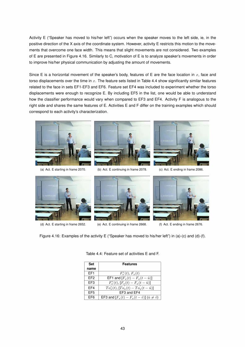
Activity E (“Speaker has moved to his/her left”) occurs when the speaker moves to the left side, ie, in the
positive direction of the X axis of the coordinate system. However, activity E restricts this motion to the move-
ments that overcome one face width. This means that slight movements are not considered. Two examples
of E are presented in Figure 4.16. Similarly to C, motivation of E is to analyze speaker’s movements in order
to improve his/her physical communication by adjusting the amount of movements.
Since E is a horizontal movement of the speaker’s body, features of E are the face location in x, face and
torso displacements over the time in x. The feature sets listed in Table 4.4 show significantly similar features
related to the face in sets EF1-EF3 and EF6. Feature set EF4 was included to experiment whether the torso
displacements were enough to recognize E. By including EF5 in the list, one would be able to understand
how the classifier performance would vary when compared to EF3 and EF4. Activity F is analogous to the
right side and shares the same features of E. Activities E and F differ on the training examples which should
correspond to each activity’s characterization.
(a) Act. E starting in frame 2070. (b) Act. E continuing in frame 2078. (c) Act. E ending in frame 2086.
(d) Act. E starting in frame 2652. (e) Act. E continuing in frame 2668. (f) Act. E ending in frame 2676.
Figure 4.16: Examples of the activity E (“Speaker has moved to his/her left”) in (a)-(c) and (d)-(f).
Table 4.4: Feature set of activities E and F.
Set FeaturesnameEF1 F v
x (t), Fx(t)
EF2 EF1 and [Fx(t)− Fx(t− u)]EF3 F v
x (t), [Fx(t)− Fx(t− u)]EF4 Tov
x(t), [To′x(t)− To
′x(t− u)]
EF5 EF3 and EF4EF6 EF3 and [Fx(t)− Fx(t− v)] (u 6= v)
43

Activity Sliding Window
A sliding window of an activity is seen as the number of frames or a time period in which an activity can occur,
ie, the assumed optimal number of frames whose features are needed to detect an activity. This way, an
activity is considered to have a start and an end times (or frames). Some activities can take some seconds,
while others can take just a small time fraction, ie, some frames.
From the Ground Truth (GT) classifications, one can observe that activity A often takes from 7 to 31 frames
to occur and 15 on average, on a video sequence at 25 fps. Activity B, on the other hand, requires a single
frame because it is only needed to check if the face is visible. Activities C and D are mostly dependent on the
hand location and not on its motion, so they require a single frame. Activities E and F could take at least 11
frames (0.44 seconds).
Feature Vector
Two methods for building the feature vector were developed. Method 1 is suitable to create feature vectors
which include the complete evolution of the activity, ie, from beginning to activity’s end. On the other hand,
Method 2 is suitable to create vectors for those activities which are not dependent on the movement’s varia-
tion, ie, activities which can be seen in a single frame.
Let M = j − i + 1 be the frames number of a training example, where i and j are the numbers of the
first and last frames of the example, respectively. Let also fl be the feature vector of frame l and K is the
sliding window size. Each feature vector Vα is given by:
Vα = fu ∪ fu+1 ∪ · · · ∪ fu+K−2 ∪ fu+K−1. (4.52)
In Method 1, u = [i+ α K, i+M −K] and α = [0, MK − 1] (α ∈ N), while in Method 2, u = [i, i+M −K]and α = u. In both methods, Vα is built if the following constraint is satisfied:
M ≥ K (4.53)
because it is required to collect features from at least K frames. In Method 1, the number of vectors Vα built
is MK , while Method 2 builds i+M −K vectors. The test vector V is defined as
V = fu−K+1 ∪ fu−K+2 ∪ · · · ∪ fu−1 ∪ fu (4.54)
where u is the current frame. Activities may occur several times without interruption, ie, an activity may be de-
tected in ∆ consecutive feature vectors where ∆ ≥ 2. In this case, only one activity is considered. Therefore,
an activity a whose discrete interval is [u −K + 1, v] is considered to have started at frame u −K + 1 and
ended at frame v = u+ ∆− 1.
One advantage of Method 2 is that it provides more vectors than Method 1, hence more training informa-
tion with only one activity example. Despite that, in many training examples MK < 2, so only one vector is
created. Therefore, Method 1 guarantees that Fα includes the activity motion evolution from its beginning,
and do not start another vector after it. Otherwise, there could result in vectors that do not represent correctly
to the activity motion.
4.3.2 Classification AlgorithmsThe classification algorithms used to create the activity classifiers are SVM and Normal Bayes, available in
OpenCV [Inte 99]. Another useful algorithm such as K-Nearest Neighbors was not fully available, so it was
44

not used. SVM and Normal Bayes are able to recognize patterns from feature vectors and they are suitable
to create binary classifiers as needed in this work. They were also chosen because no implementation effort
was required. These algorithms are briefly explained below.
Support Vector Machines (SVM)SVM is a supervised learning method which was originally developed for binary classification of data. It
was then extended to regression and clustering [Wiki 09b, Will 09b]. Input data are two sets of vectors in
a n-dimensional space. Its goal is to assign (classify) a test data vector x ∈ R2 into one of two classes
yi ∈ −1, 1, where each class is associated with each vector set. Input data xi, where i denotes the i-th
training vector, is used as training set, so the algorithm learns from it to distinguish between the two classes.
The SVM method builds an hyperplane H which separates the two sets of vectors. H is given by w · x+b = 0and it should maximize the margin (distance) 1
||w|| between the two classes (see Figure 4.17). w is normal
to H, b is a distance offset from H to the origin and · is the dot product. In order to obtain the margin, the
algorithm creates two parallel hyperplanes (H1, H2) over the closest vectors to H. The vectors lying on H1 or
H2 are called support vectors and these are used to calculate the class yi of each test vector. Each training
vector i belongs to class yi if it satisfies
yi(xi · w + b)− 1 ≥ 0, ∀i. (4.55)
The margin is maximized by minimizing ||w|| subject to (4.55). The generalization error of data classification
decreases as the margin increases. Figure 4.17 shows an example of linear data separation with two data
sets (black and white circles) in R2 and the hyperplanes H, H1 and H2.
In [Cort 95], Cortes et al. presented the Soft Margin method which deals with cases where the training
Figure 4.17: Example of a separable problem R2 with SVM. Support vectors are identified with an extra circle.The two data classes are separated by hyperplanes H, H1, and H2.
data cannot be linearly separated without error. Instead, it separates data with a minimal number of errors. It
introduces non-negative slack variables ξi which measure the degree of misclassification of xi. The margin
is obtained by minimizing12||w||2 + C F
(n∑i=1
ξi
)(4.56)
45

where n is the number of training vectors, C is a constant and F (u) is a monotonic convex function with
F (0) = 0. (4.56) is subject to yi(xi · w + b) ≥ 1 − ξi and ξi ≥ 0, ∀ i. C controls the trade-off between
the margin size and the training error. A small C causes a higher margin, but ignores the existing outliers; a
large C gives a higher penalty on the errors, but the classifier may suffer from overfitting. The methods above
handle linear classifications. However, data distribution in space is often non-separable by linear functions.
This problem has been overcome by applying the Kernel trick. The main idea is to map each xi to another
feature space with a non-linear function Φ and finally, apply the previous linear algorithm to Φ(xi). Most
common kernel functions are Radial Basis Function (RBF), Polynomial, Gaussian Radial Basis function and
sigmoid function. The kernel function k used in this work was RBF as expressed below:
k(x, x) = e−γ|x−x|2 . (4.57)
SVM limitations are the kernel choice which is hard to choose when no prior knowledge is available; discov-
ering the kernel best parameters for the task in hands; time and speed to train and test present limitations,
mainly in training very large data sets; and the optimal design for multi-class SVM classifiers was not yet
achieved [Burg 98].
Normal Bayes
Normal (or Naive) Bayes is an algorithm which was applied on machine learning. It relies on a simple model
that assumes the feature vectors from each class are normally distributed [Will 09a] and independent from
each other. Thus, the data distribution function is assumed to be a Gaussian mixture, one component for
each class. From the training data, the algorithm estimates mean vectors and covariation matrices for each
class, and uses them for classifying the feature vector with a specific class. In the algorithm available in
[Inte 99], the data are not necessarily independently distributed. The Naive Bayes classifier combines the
Bayes’ probability model with a decision rule by choosing the most probable hypothesis (class), known as the
maximum a posteriori decision rule [Wiki 09a]. The classifier Λ is given by the following expression:
Λ(F ) = arg maxc
p(C = c)n∏i=1
p(Fi = fi|C = c) (4.58)
where p(C = c) is the prior probability of having a vector belonging to class c, p(Fi = fi|C = c) denotes the
probability distribution, and F is the feature vector. Naive Bayes classifier is simple, requires low computa-
tional effort and requires small amounts of training data to estimate the parameters for classifying. However,
it assumes fully independent features which fails for complex classification problems. Besides, it fails on
separating most of non-linearly distributed data.
4.3.3 Train and TestThe classifier is trained after characterizing the activity, choosing the classification algorithm and labeling the
selected examples. Firstly, the system runs every video sequence from the training set. Then, for each se-
quence the tracker locates speaker’s body parts and for each training example, the activity recognition module
converts speaker’s body regions into features (Feature Conversion in Figure 4.1) and puts these features in
vectors (Collection of Features). The training is finally performed after the system has collected features from
all the video samples (Train). The training output is a model file which is used by the classification algorithm
when it classifies some feature vector.
After training all the classifiers, the system is ready to be used for activity recognition and its performance
can be evaluated using the test set. The tracker gives the body locations and the activity recognition module
runs all the activity classifiers. Each one of these classifiers collects its own specific features until the feature
46

vector is full. Then, the vector is given to the classifier as test data and the classifier reports if its activity has
occurred, based on its training. This process repeats from the image capture until the video sequence ends.
The parameters that influence the classifier performance are the features used, the sliding window size,
the method for building the feature vector, the classification algorithm and also the training examples. The
best set(s) of parameters for each activity are not easily obtained. Still, by evaluating several sets, the best of
them can be obtained.
4.4 Video RecordingVideo recording module includes two recording operations. Since saving the presentation video for later view-
ing is a requirement of the system, this module continuously records the full captured image in the original
resolution (see Figure 4.18(a)). Moreover, in the presentation images, the speaker occupies only a small
area and the remaining area gives no interesting information about the presentation. Thus, another video
sequence centered in the speaker’s body is recorded (Figure 4.18(b)).
The algorithm which provides the smaller image region starts by computing the smallest image region RS
(a) Full image (b) Clipped imagewith ρw = 0.35
Figure 4.18: Example of the recorded images in every frame.
that contains the face, hands and torso regions. One pretends to record only this region, but its size RSd is
not constant because the speaker may show different body poses, and the video recording tool of OpenCV
[Inte 99] requires a constant region size. Accordingly, the size RVd (width and height) of each recorded image
should be previously defined as:
RVd = (ρw W,ρh H) (4.59)
where ρw, ρh ∈ ]0, 1] denote the image’s size rate that will be recorded around the speaker’s body. ρw and ρhwere set as 0.5 and 1, respectively. Once RVd is computed, the recorded region center RVc is defined as the
center of RS (RSc ).
4.5 DiscussionWhen designing the tracking algorithm, the author wanted it to be precise in its body estimations, easy to
understand and implement, fast and resolution independent. Generally, these goals were achieved. In this
section, the decisions that led to the proposed solution are discussed and explained. It is also given an
47

analysis on some relevant issues related to tracker performance and how some parameters may be changed
to adapt the system functioning. At the end, the activity recognition process is discussed and the system
capabilities, limitations and supporting technology are described.
4.5.1 Image Resolution and ScalabilityOriginal image resolution is 360x288 and the tracking system uses by default a reduced image resolution of
90x72 (W = 90, H = 72). Reducing the image maintains tracking capabilities and speeds up the system
because there are less pixels to process. The tracker also works with 360x288 and 180x144. For 45x36
images, the tracker is able to track the face and torso, but not the hands since there is few visual information.
The tracking algorithm is scalable since it is prepared to cope with higher resolution images. If the image
ratio gets changed, one only needs to redefine the expected speaker’s scale (parameters υ1 and υ2). For the
resolution used , β1 is 9, but for other image resolutions β1 = 9 ( rd)2, where r = 4 is the ratio between original
and default resolution, and d ∈ [1,min(W,H)] is a reduction factor.
4.5.2 Processed FramesIn the proposed system, to perform tracking all frames are processed. Nevertheless, tracking algorithm is
flexible enough to work with non-consecutive frames. In this case, a fast face and/or hand movement puts
these body parts away from the previous location and out of the search regions (RF and RHa) at time t. Even
so, search regions are easily adapted by increasing parameters β3, β4 and ψ5. Increasing search regions
increases pixels to process hence the processing time; processing non-consecutive frames balances this time
increase.
4.5.3 Human ProportionsKnowledge about human proportions is essential to keep the tracked body parts proportional to each other,
eliminating blobs that do not match the proportion. It also allows to reduce the body search regions in the
image and to avoid processing data that cannot be associated to speaker’s body.
4.5.4 Background SubtractionIn the BS algorithm, as a way of building an accurate background model, the speaker should not be in
the image at the presentation beginning. However, the tracker is still able to track the speaker even if this
assumption is not verified. Even if the speaker moves slightly after the creation of the model, this motion will
suffice to obtain the region where he/she moves, unless the audience is more dynamic than the speaker. A
more dynamic audience at the beginning may lead the algorithm to track the audience. Still, it is preferable
not having the speaker at the beginning.
4.5.5 Skin DetectionFace and hand detection heavily depend on skin detection. Therefore, the proposed system is also dependent
on skin detection which requires using an accurate skin detector. Figure 4.19 compares five skin classifiers
by showing their results over five images taken from real presentations. The classifiers are based on RGB
and HSV color spaces and they were denoted by RGB1, RGB2, RGB3, HSV1 and HSV2. RGB1, RGB2 and
RGB3 are defined in (2.5), (2.6) and (2.7), respectively. Using HSV1, a pixel is classified as skin (for Asian
and Caucasian ethnics) if the H ∈ [0, 0.2777] and S ∈ [0.23, 0.68], where H and S are the hue and saturation
channels [Oliv 09]. HSV2 classifies a pixel as skin if H ∈ [0, 0.11] and S ∈ [0.2, 0.7] [Stil 07].
From Figure 4.19, one observes that RGB1 and RGB3 provide identical results and also the best perfor-
mance. Figures 4.19(a), 4.19(e), 4.19(i) and 4.19(m) show that RGB1 overcomes HSV1 because it detects
more skin and it is more accurate. HSV2 detects more skin than HSV1 and RGB1 and recalls most of the
48
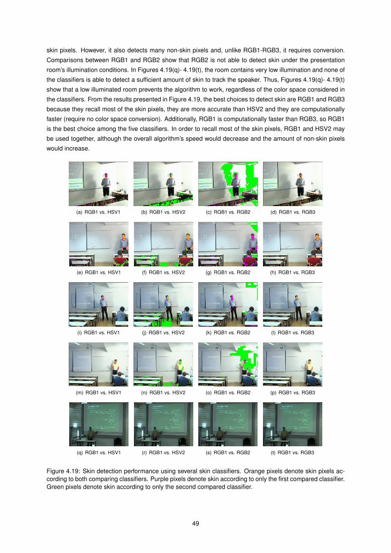
skin pixels. However, it also detects many non-skin pixels and, unlike RGB1-RGB3, it requires conversion.
Comparisons between RGB1 and RGB2 show that RGB2 is not able to detect skin under the presentation
room’s illumination conditions. In Figures 4.19(q)- 4.19(t), the room contains very low illumination and none of
the classifiers is able to detect a sufficient amount of skin to track the speaker. Thus, Figures 4.19(q)- 4.19(t)
show that a low illuminated room prevents the algorithm to work, regardless of the color space considered in
the classifiers. From the results presented in Figure 4.19, the best choices to detect skin are RGB1 and RGB3
because they recall most of the skin pixels, they are more accurate than HSV2 and they are computationally
faster (require no color space conversion). Additionally, RGB1 is computationally faster than RGB3, so RGB1
is the best choice among the five classifiers. In order to recall most of the skin pixels, RGB1 and HSV2 may
be used together, although the overall algorithm’s speed would decrease and the amount of non-skin pixels
would increase.
(a) RGB1 vs. HSV1 (b) RGB1 vs. HSV2 (c) RGB1 vs. RGB2 (d) RGB1 vs. RGB3
(e) RGB1 vs. HSV1 (f) RGB1 vs. HSV2 (g) RGB1 vs. RGB2 (h) RGB1 vs. RGB3
(i) RGB1 vs. HSV1 (j) RGB1 vs. HSV2 (k) RGB1 vs. RGB2 (l) RGB1 vs. RGB3
(m) RGB1 vs. HSV1 (n) RGB1 vs. HSV2 (o) RGB1 vs. RGB2 (p) RGB1 vs. RGB3
(q) RGB1 vs. HSV1 (r) RGB1 vs. HSV2 (s) RGB1 vs. RGB2 (t) RGB1 vs. RGB3
Figure 4.19: Skin detection performance using several skin classifiers. Orange pixels denote skin pixels ac-cording to both comparing classifiers. Purple pixels denote skin according to only the first compared classifier.Green pixels denote skin according to only the second compared classifier.
49

4.5.6 Body TrackingSection 2.6.4 provides a representative set of tracking techniques which were considered when building the
algorithm. Hereafter, an analysis of reviewed tracking techniques/systems shows some drawbacks which
make them unsuitable to the described problem. Later, some comments related to body tracking are given.
A similar algorithm to Pfinder does not solve the current problem because it does not handle sudden illu-
mination changes, large audience movements, or lack of contour points, if the speaker’s clothes present low
contrast on the background. However, Pfinder has inspired the proposed algorithm with the blob concept for
face and hands. Mean Shift tracker [Coma 01] was seen as unsuitable due to its sensitivity to illumination and
lack of scale adaptation; however it was tested. Coupled CAMSHIFT [Brad 98] improves Mean Shift, but its
results have shown to be unsatisfactory. Ramanan et al. have developed a very advanced tracking system,
but also hard to implement and not suitable to track hands over the torso. The inability to track hands in this
pose, led to also exclude skeleton tracking. Another tracking approach is based on body part detectors. This
would be a simple but slow algorithm, if these detectors were available. Even if those detectors were trained,
they would require a lot of effort, time, training examples and tools, and there would be no guarantee of high
detection rates.
Although this tracking algorithm has been designed to handle a single person facing the camera, it is able to
keep tracking even if another person appears. Since body parts are only searched for in the neighborhood
of previous locations, a new person in the image will not affect the tracker, unless both people become too
close or the tracker loses face location in that moment. Below, it is presented an analysis on alternative body
tracking approaches and related decisions which were made for each body part.
Face Tracking
When developing face tracking component, three approaches were made, besides the one presented above.
The first one combines the face detector (FD) from OpenCV with skin detection, so that a region provided by
the FD, had to contain a certain amount of skin. This technique is simple, provides an accurate face scale
and requires less development effort compared to the developed one. However, the OpenCV’s face detector
makes the algorithm slower and the face scale in I is often very small, causing no face detections most of the
time. Besides, in a presentation there is no guarantee that there will be always a face frontal view, so this FD
is less reliable than the proposed algorithm. Although its disadvantages, this technique is also available in the
system as an alternative face detection method. The system user can easily choose between face detection
through skin blobs or the OpenCV method. The second alternative combines Mean Shift tracker with skin
detection. Experimental tests show that it is able to track the speaker when he/she is in the image, but it does
not adapt to face scale, it is sensitive to illumination changes and loses the face if a close object has a similar
color appearance. Third approach has combined Coupled CAMSHIFT with skin detection. It adapts to scale
and illumination, but it also has shown to be unable to track the speaker. After skin blob algorithm detects
the face blob, Coupled CAMSHIFT rapidly starts tracking another image region. In the presented algorithm,
RFh could be reduced to its half because the face is expected to appear in the top half of the image, although
it is safer to do this only if the background model includes most of the speaker; otherwise reducing RFh may
cause losing the image region where the face is visible. For hand tracking, the behavior of the second and
third approaches is the same.
Torso Tracking
As alternative approaches for torso, detection was achieved with the proposed algorithm and tracking was
based on the previous Mean Shift algorithms. The results of three alternative approaches and also the pro-
posed algorithm are shown in Figures 4.20-4.21. In Figure 4.20 there is a low contrast between the person’s
50

clothes and the room background whereas in Figure 4.21 the contrast is low. Using Mean Shift tracker, To is
not as accurate as the proposed algorithm provides (compare Figures 4.20(a) and 4.20(e)). Note that the MS
tracker tends to move to a less accurate region in Figures 4.20(c)-4.20(e) or to settle down on a given region
(Figure 4.21(b)). In addition, its scale does not adapt to the speaker’s pose. Using Coupled CAMSHIFT,
an approximate region shown in Figure 4.20(f) rapidly grows and is replaced by another image region (Fig-
ures 4.20(g)-4.20(h)). Figures 4.21(c)-4.21(e) also show a too large and fixed torso region, so this algorithm
shows to be ineffective.
(a) Proposed algorithm appliedto frame 757 (see Section 4.2.3)
(b) Mean Shift and pyramid seg-mentation applied to frame 757where To is a very small regionover the speaker’s waist
(c) Torso detection with the pro-posed algorithm in frame 502
(d) MS tracking in frame 503 (e) MS tracking in frame 757
(f) Torso detection with the pro-posed algorithm in frame 510
(g) CAMSHIFT in frame 512 (h) CAMSHIFT in frame 514
Figure 4.20: Results of four torso tracking techniques: proposed algorithm (4.20(a), 4.20(c), 4.20(f)),Mean Shift + Pyramid Segmentation (4.20(b)), Mean Shift tracker (4.20(d)-4.20(e)) and Coupled CAMSHIFT(4.20(g)-4.20(h)). In the figures, the colors of the person’s shirt are similar to the room background preventingthe MS + Pyramid Segmentation algorithm to correctly estimate To. Torso region is the yellow rectangle.
Finally, a third torso tracking approach was taken. It segments the expected torso region (below the face)
through Mean Shift and pyramid segmentation [Krop 96], resulting on a few smoothed regions, although a
perfect segmentation would result on a single region. Then, some color samples from below the face are
collected and the similarity between these samples and each smoothed region is computed. The most similar
region is considered to be the torso region. Although this approach may yield better results than the Mean
Shift-based algorithms (see Figures 4.21(f)-4.21(g)) and provide competitive results with the proposed algo-
rithm (Figure 4.21(a)), it has also shown to require a high contrast between torso clothes and background. As
a consequence, it is not able to tracker the speaker’s torso in Figure 4.20(b).
51
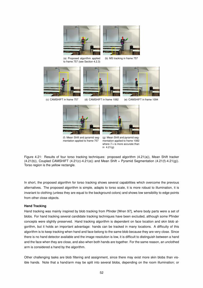
(a) Proposed algorithm appliedto frame 757 (see Section 4.2.3)
(b) MS tracking in frame 757
(c) CAMSHIFT in frame 757 (d) CAMSHIFT in frame 1082 (e) CAMSHIFT in frame 1094
(f) Mean Shift and pyramid seg-mentation applied to frame 757
(g) Mean Shift and pyramid seg-mentation applied to frame 1082where To is more accurate thanin 4.21(g)
Figure 4.21: Results of four torso tracking techniques: proposed algorithm (4.21(a)), Mean Shift tracker(4.21(b)), Coupled CAMSHIFT (4.21(c)-4.21(e)) and Mean Shift + Pyramid Segmentation (4.21(f)-4.21(g)).Torso region is the yellow rectangle.
In short, the proposed algorithm for torso tracking shows several capabilities which overcome the previous
alternatives. The proposed algorithm is simple, adapts to torso scale, it is more robust to illumination, it is
invariant to clothing (unless they are equal to the background colors) and shows low sensibility to edge points
from other close objects.
Hand Tracking
Hand tracking was mainly inspired by blob tracking from Pfinder [Wren 97], where body parts were a set of
blobs. For hand tracking several candidate tracking techniques have been excluded, although some Pfinder
concepts were slightly preserved. Hand tracking algorithm is dependent on face location and skin blob al-
gorithm, but it holds an important advantage: hands can be tracked in many locations. A difficulty of this
algorithm is to keep tracking when hand and face belong to the same blob because they are very close. Since
there is no hand detector available and the image resolution is low, it is difficult to distinguish between a hand
and the face when they are close, and also when both hands are together. For the same reason, an unclothed
arm is considered a hand by the algorithm.
Other challenging tasks are blob filtering and assignment, since there may exist more skin blobs than vis-
ible hands. Note that a hand/arm may be split into several blobs, depending on the room illumination; or
52

there may exist skin-like objects around the speaker. Default hand helps filtering skin blobs, but hand scale
shows large variations which depend on speaker gestures. Hand tracking algorithm always tries to assign
blobs to both hands, which leads to assignment errors when both hands are together and another skin blob
was detected around the speaker. In this situation, both hands blob is assigned to a given hand and the
another existing blob is wrongly associated with the other hand. In order to maximize correct hand tracking,
the algorithm requires no skin-like objects around the speaker.
4.5.7 Activity RecognitionActivity recognition module was specifically designed to support any kind of activity based on visual features,
regardless the activity complexity. Therefore, adding new activities is easy since the training and testing pro-
cess is generic for all the activities. For example, activity B would be easily recognized by checking if the
face location was known. However, for other activities there are no simple rules to check. Thus, supervised
learning allows each activity classifier to learn each activity behavior and decide from the given features. This
approach is activity independent and saves significant effort when a new activity is added.
In activity recognition the most critical tasks are training set labeling and choosing the feature sets. From
previous experimental tests, one may observe significantly different results from very similar training data.
Depending on the activity characteristics, it is possible to deduce some of the required features. However,
a complete features set is obtained after comparing the classifier performance with several feature sets. In
addition, activity recognition module relies on tracker performance, assuming it is accurate.
4.5.8 Capabilities and LimitationsThe proposed system has a set of capabilities and also some limitations. These are listed below.
Capabilities
The system has the following capabilities:
• Track speaker’s face, both hands and torso.
• Distinguish left and right hands from some assumptions.
• Recognize a set of activities.
• Record the presentation in video.
Limitations
The algorithm’s limitations are the following:
• To track correctly the hands, speaker’s clothes of the upper body and the room background must not
be skin-like. Red, orange and brown are mostly skin-like, according to the skin classifier, and therefore,
these colors difficult hand tracking.
• Tracking algorithm requires no skin-like objects or students’ body parts around the speaker’s body; it is
one of the algorithm’s assumptions. Tracking algorithm assumes that the skin-like regions around the
speaker belong to his/her body parts and not to other objects. Nevertheless, the algorithm is tolerant to
other skin-like objects and still tracks hands.
• If a hand becomes too close to the head, the system only tracks one of them because they belong to
the same skin region and there is no face or hand detector to distinguish between them.
• Tracking algorithm is a single person algorithm. When multiple people are facing the camera, only one
is tracked since the algorithm was designed to the presentation environment where it is assumed that a
single person is facing the camera.
53

• Background model requires some seconds to be built, depending on W , H , N and T . One should
ensure that background model is built before the speaker enters the scene to improve tracking and also
activity recognition.
4.5.9 TechnologyThe system was developed in C++ using Microsoft Visual Studio 2005. Image processing was made easier by
using OpenCV1.1 library [Inte 99]. OpenCV is a cross-platform computer vision library. The use of OpenCV
led to C++, since it is mainly developed to C/C++, although other languages such as Java, Python and
C# (OpenCV wrapper) can be used. In addition, C++ allows creating faster applications than the previous
programming languages, which is an important issue when trying to achieve real-time processing. This system
uses OpenCV’s machine learning algorithms, Canny’s edge detector [Cann 86], procedures to capture and
record video, and data structures. OpenCV does not support recording both video and audio into a file, so the
recording module includes only the video data. OpenCV presents the following advantages:
1. dedicated computer vision library;
2. simple programming interfaces;
3. hundreds of computer vision algorithms available;
4. free for commercial and research use under a BSD license;
5. library in continuous development;
6. has a large community of users and forums for problem discussion;
7. many available code examples;
8. little CV knowledge is enough for simple programs;
9. includes algorithms for person tracking systems (Mean Shift, Coupled CAMSHIFT, Viola and Jones face
detector, Canny’s edge detector).
On the other hand, OpenCV has some disadvantages such as:
1. integration required;
2. contains bugs and incomplete features which are hard to correct/complete for a common user;
3. some basic procedures/data structures need to be improved to reduce programming effort and errors;
4. does not provide a feature to record both video and audio information;
5. the existing GUI is not sufficient to an user that needs an application with menus and buttons;
6. often there is reduced documentation or the documentation is outdated.
Another image processing toolbox was available in MATLAB [Inc 94], but comparing with OpenCV, it shows
many disadvantages, such as less computer vision algorithms available, less support (documentation and
code examples), it is not free, and its interface is harder to learn for a C++ user. Besides, MATLAB also
requires integration in the application.
54

4.6 ConclusionsIn this chapter, the proposed system is described in detail. It covers speaker tracking, activity recognition,
video recording, and provides a discussion on the algorithms. Speaker’s face is obtained by detecting a
square skin blob. Torso left and right boundaries are given by the median edge points below the face, given
by Canny’s edge detector. Hands are considered the biggest skin regions close to the face and torso, which
satisfy a set of rules. Each activity is recognized by using a binary classifier. The classifier learns the activity
from a data set which includes positive and negative examples of the activity. Video recording module simply
saves the video in the original resolution and a clipped video which mainly shows the speaker.
Comparing state-of-the-art tracking techniques with the developed algorithms, one can perceive that these
techniques are not suitable to solve the formulated problem, given the system requirements. As mentioned at
the beginning of this chapter, each solution depends on each scene conditions and assumptions. Therefore,
this solution was designed after an analysis of the system requirements and the capabilities of the available
techniques.
For activity recognition, there was a very acceptable variety of classification algorithms to choose. Besides, all
of them have already shown to be effective in activity recognition. In this system, the activity set included not
very complex activities, so the classification algorithm choosing was mainly related to its ability to recognize
patterns, its suitability to a binary classification, and its availability on a programming library.
55

Chapter 5
Experimental Results
5.1 IntroductionThis chapter presents an experimental evaluation of the proposed system. Experimental results include the
evaluation of the tracking algorithm performance, the activity classifiers performance and the system’s speed.
The proposed system was evaluated on a database of 73 video sequences with a total duration of 2 hours,
20 minutes and 16 seconds and the performance was measured using a set of objective metrics. The video
database and the metrics will be presented in the next sections. A discussion on the results is included at the
end of this chapter.
5.2 Video Data SetA set of video sequences was extracted from real presentations containing different speakers and two video
sequences were captured in a presentation room, but they are not part of a presentation; these two sequences
were used as negative examples of the activities. The video data set was used as a test set for tracking, and
as a training and test set for activity recognition. These video sequences were divided into three groups
according to their purpose. Group 1 contains 5 sequences (see Table B.1 on Appendix B) that were used to
test the tracker’s performance with different presentations and speakers. Group 2 contains 5 sequences (Ta-
ble B.2) for measuring the tracker performance under different illumination conditions. Group 3 is the training
and test set for activity recognition and includes 63 sequences (Tables B.3- B.5). In Group 3, each sequence
may be used to train/test one or more activity classifiers depending on its content.
Sequences of Groups 1 and 2 were randomly selected from the presentations that contain different speakers
and illumination conditions, respectively. Sequences of Group 3 were chosen after verifying that the tracker
could track fairly well during the activities occurrence, providing good features for the training and testing.
These sequences were also chosen because they contained more often each activity than the other pre-
sentation subsequences. Sequences from Group 3 were taken from presentations given in the same room
(“Room1” - see Section 5.2.1) and by the same speaker. All video sequences have a 360x288 resolution at
25 fps and they were captured with a camera Canon XL2.
Next sections describe the room characteristics where the presentations were made, the data labeling pro-
cess and the training and test process for activity recognition.
5.2.1 Illumination and Room CharacteristicsIn sequences “9”, “29”, “30”, “69”, “70” from “presentation1” and “10” from “presentation2”, the presentations
were made in large rooms with capacity for about 90 people. In ”presentation1” there is plenty illumination
which is provided by the lamps in the ceiling. In “10” there is little illumination, the lamps in the ceiling are
56
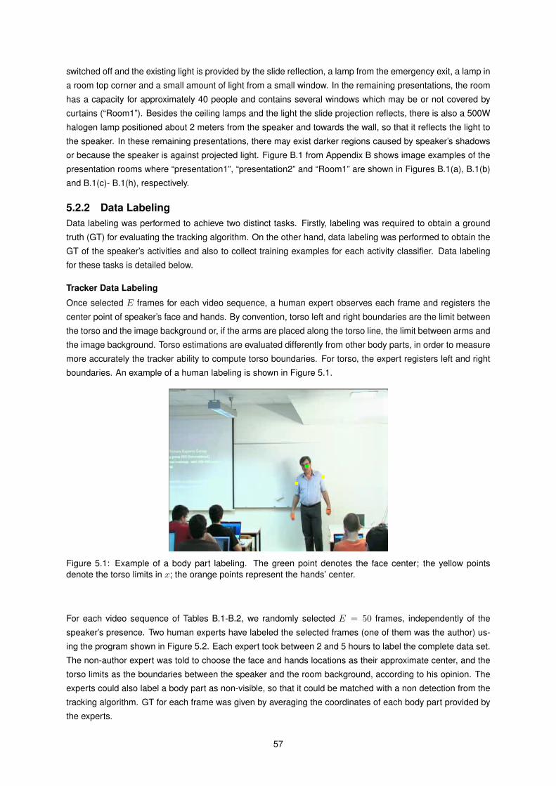
switched off and the existing light is provided by the slide reflection, a lamp from the emergency exit, a lamp in
a room top corner and a small amount of light from a small window. In the remaining presentations, the room
has a capacity for approximately 40 people and contains several windows which may be or not covered by
curtains (“Room1”). Besides the ceiling lamps and the light the slide projection reflects, there is also a 500W
halogen lamp positioned about 2 meters from the speaker and towards the wall, so that it reflects the light to
the speaker. In these remaining presentations, there may exist darker regions caused by speaker’s shadows
or because the speaker is against projected light. Figure B.1 from Appendix B shows image examples of the
presentation rooms where “presentation1”, “presentation2” and “Room1” are shown in Figures B.1(a), B.1(b)
and B.1(c)- B.1(h), respectively.
5.2.2 Data LabelingData labeling was performed to achieve two distinct tasks. Firstly, labeling was required to obtain a ground
truth (GT) for evaluating the tracking algorithm. On the other hand, data labeling was performed to obtain the
GT of the speaker’s activities and also to collect training examples for each activity classifier. Data labeling
for these tasks is detailed below.
Tracker Data Labeling
Once selected E frames for each video sequence, a human expert observes each frame and registers the
center point of speaker’s face and hands. By convention, torso left and right boundaries are the limit between
the torso and the image background or, if the arms are placed along the torso line, the limit between arms and
the image background. Torso estimations are evaluated differently from other body parts, in order to measure
more accurately the tracker ability to compute torso boundaries. For torso, the expert registers left and right
boundaries. An example of a human labeling is shown in Figure 5.1.
Figure 5.1: Example of a body part labeling. The green point denotes the face center; the yellow pointsdenote the torso limits in x; the orange points represent the hands’ center.
For each video sequence of Tables B.1-B.2, we randomly selected E = 50 frames, independently of the
speaker’s presence. Two human experts have labeled the selected frames (one of them was the author) us-
ing the program shown in Figure 5.2. Each expert took between 2 and 5 hours to label the complete data set.
The non-author expert was told to choose the face and hands locations as their approximate center, and the
torso limits as the boundaries between the speaker and the room background, according to his opinion. The
experts could also label a body part as non-visible, so that it could be matched with a non detection from the
tracking algorithm. GT for each frame was given by averaging the coordinates of each body part provided by
the experts.
57

Figure 5.2: Interface of the program to collect the tracker’s GT. The human expert chooses each body partlocation.
Activity Data Labeling
Labeling of activity examples for testing was performed by three human experts (including the author). The
complete data sets of activities A, B, D, E and F were labeled twice by two experts. Data set of C was also
labeled twice, but one of the labellings was shared by two experts. The time required to label the complete
data set of each activity mainly depended on the sequence’s length, the number of activity occurrences and
on the expert’s speed. To label the data set of activities A-F, each expert took 40 minutes-2 hours (A), 5-10
minutes (B), 20-30 minutes (C), 1-3 hours (D), 13-25 hours (E) and 4-8 hours (F). The experts were taught
to recognize each activity from image examples and from counterexamples given by the author as shown in
Figure 5.3 for activity D.
Each expert has carefully observed the selected video sequences in VirtualDub (see Figure 5.4) and very
often the experts had to forward and rewind the video frames in order to check the “correct” start and end
frames of the activities. Each activity occurrence has been stored with the format:
< video sequence id >:< label >< start frame >:< end frame >
where < video sequence id > is the video sequence name, < label > is the example label (positive or
negative), < start frame > is the first frame of the video sequence where the activity is observed, and
< end frame > is the last frame of the activity. Since the expert only stores positive examples, < label > =
58

Figure 5.3: Counterexample of activity D (“Speaker is pointing to his/her right”).
1. For training, the author has selected a subset of the labeled examples where the tracker is able to track the
speaker. This avoids providing features which do not correspond to an activity occurrence or at least reduces
the number of wrong examples. Since the experts have only labeled positive examples, the author has labeled
some negative examples from the video sequences and set < label > as -1 (see Tables B.3- B.5).
Figure 5.4: Program used to observe the activity occurrences (VirtualDub). The human expert chooses thefirst and last frames of each activity occurrence and writes it.
GT was obtained by a selective merging of the experts’ labellings (classifications) in the format above. Firstly,
the classifications where the experts’ opinions completely differed were manually analyzed. Differences in
classifications may be caused by different criteria or the expert may have unintentionally missed an activity
occurrence. Those activity occurrences only labeled by an expert and which do not correspond to the activity
characteristics were not considered. Secondly, the remaining classified occurrences of each video sequence
and activity were merged as follows. Let Ei be the classified activity occurrences by expert i for an activity a
and video sequence v. Let Eit = 1 when the expert considers that a is occurring in time t of v, and Eit = 0
59

otherwise. GT of activity a, sequence v and frame t (denoted by GT vt ∈ 0, 1) is given by
GT vt =
1,E∑i=1
Eit ≥ Th
0, otherwise
(5.1)
where E = 2 is the number of experts and Th = 1 denotes the minimum number of experts that consider
Eit = 1. Then, GT for each sequence v is defined as follows:
GT v = GT v0 , · · · , GT vT −1 (5.2)
where T is the frame number of sequence v. Finally, the consecutive frame elements of GT v where GT vt = 1are transformed into discrete intervals which depict the starting and ending frames of an activity occurrence.
These intervals are posteriorly used in (5.7). Each interval is denoted by aGT .
5.2.3 Training and Test SetsActivity examples for activity recognition were collected from several presentation video sequences. These
examples were split into two sets: training and test set. These sets are disjoint, in order to test the classifier
ability to detect the activity with different examples.
Training and test sets were defined by 5-fold cross validation. Accordingly, each activity data set was di-
vided into N disjoint subsets (N = 5). The training set contains N - 1 subsets and the test set contains the
remaining subset. Usually, each subset includes 2-4 video sequences. This procedure was repeated N times
rotating the test set. The classification performance is the average of the N tests performance. Some video
sequences contain mostly negative examples. In order to provide a sufficient number of negative examples
to each subset, instead of putting them in the same subset, the sequences of each subset were chosen so
that the number of positive and negative examples was balanced. In the data set, negative examples of an
activity may include several other activities.
5.3 Tracking EvaluationEvaluation of tracking performance measures the error between tracker’s GT and the tracking algorithm es-
timations. Besides, the detection rate of speaker’s body parts is also computed. The body parts included in
these measurements are the face, torso and hands. This section presents the tracking results for different
presentations, speakers and illumination conditions. Since illumination conditions greatly affect skin detection
and the tracker performance, the developed tracker was tested under several illumination conditions. The
evaluation process consists in measuring the error between the GT and the estimations as described in Sec-
tion 5.3.1. The test set of the tracker is listed in Table B.1. Results of tracking performance are presented in
Section 5.3.2.
5.3.1 Evaluation MetricsFor each body part (face, hands, torso) we computed several metrics based on the tracking errors and a
confusion matrix. If a point is detected, we can define a tracking error e = (ex, ey) as the difference between
the estimated position s = (sx, sy) and the GT position s = (sx, sy) of a given body part (Fc, Toc, LHc or
RHc). Therefore,
e = s− s. (5.3)
60
The statistical properties of e can be characterized by computing the mean error e, standard deviation σe and
covariance matrix R as follows:
ek =1E
E∑t′=1
et′
k (5.4)
σek =
√√√√ 1E
E∑t′=1
(et′
k − ek)2 (5.5)
R =1E
E∑t′=1
(et′
k − ek)(et′
k − ek)T (5.6)
where k = x, y and t′ denotes the frame sample number. The detection probability of the body points
is measured through a confusion matrix which contains four probabilities. A confusion matrix M presents
the detection probability of the body points, comparing tracker’s estimations and GT. M(m, n) denotes the
probability that a body point is estimated with label n, given the GT label m.
5.3.2 Tracking PerformanceThe results for each body part and image resolution are shown in Tables 5.1-5.4. The tables below present
the measured values of e for coordinates (x, y), R and M for face and hands. Torso values include e and
σe for torso boundaries and the confusion matrix. See also Tables C.1-C.12 on Appendix C for the complete
data of each test video. Note that the measurements in pixels presented in the tables below, were converted
to the original video resolution (360x288).
Average error e for face is low for all the image resolutions (see Table 5.1), there are no false detections
and the detection probability is between 76% and 86%. Average standard errors in (x,y), given by the square
root of the main diagonal of R, are low and mostly below 4.41 and 5.32, respectively. For resolution 180x144,
the errors are mostly very low, but an incorrect tracking in sequence “4” has caused a very high average error
(see Table C.5). In this sequence, the speaker’s clothes are skin-like and there are other skin-like objects
which are assumed to be the body parts (see Figure B.1(f) for an example of the scene). The results show
that the error is higher in the Y axis. R indicates a low correlation between x and y as these variables in-
crease. A higher error in Y and this correlation may be caused by a hand or the neck in the same skin blob.
Mostly, ex and ey increase when the face region includes other skin regions or the hand is considered the
face. Consequently, ey is higher and the correlation is positive.
Table 5.1: Average tracking performance of the speaker’s face for video sequences of Group 1.
Resolution ex ey R M(0, 0) M(1, 0)
M(0, 1) M(1, 1)90x72 0.84 4.15 19.45 1.58 1 0
1.58 26.48 0.24 0.76180x144 18.21 16.47 1502.59 930.34 1 0
930.34 643.95 0.14 0.86360x288 1.21 4.54 18.88 2.23 1 0
2.23 28.3 0.15 0.85
Torso tracking presents a low error (Table 5.2), but it is also affected by the errors in sequence “4” (see
Table C.6). Since the torso is tracked every time the face is detected, confusion matrix of both body parts is
equal. Considering that there is not an unique x coordinate for torso boundaries and the background color
is often similar to the speaker’s clothes, the obtained results are quite reasonable. From Tables 5.2, C.2, C.6
and C.10, one also observes more frequently a negative ex for the left boundary and a positive ex for the right
boundary. This shows that the image region between the estimated torso boundaries includes fewer pixels
61
Table 5.2: Average tracking performance of the speaker’s torso for video sequences of Group 1.
Resolution Right boundary Left boundary M(0, 0) M(1, 0)
ex σex ex σex M(0, 1) M(1, 1)90x72 0.23 6.07 -5.84 5.7 1 0
0.24 0.76180x144 17.22 21.93 12.8 22.17 1 0
0.14 0.86360x288 3.68 6.36 -5.1 6.8 1 0
0.15 0.85
Table 5.3: Average tracking performance of the speaker’s left hand for video sequences of Group 1.
Resolution ex ey R M(0, 0) M(1, 0)
M(0, 1) M(1, 1)90x72 3.06 -5.86 25.23 -6.88 0.93 0.07
-6.88 132.11 0.48 0.52180x144 24.33 22.27 1603.35 708.36 0.34 0.66
708.36 795.57 0.23 0.77360x288 12.73 7.71 422.78 280.99 0.22 0.78
280.99 627 0.24 0.76
than the GT boundaries’ region. The main reason to this difference is the expert labeling that often considered
the speaker’s arms as the torso boundaries. On the other hand, his/her arms often add a considerable amount
of edge points to the torso tracking algorithm. These edge points are located between the torso boundaries
and the arm’s inner boundary, and in the arm’s outer boundary, which result into two approximately vertical
edge lines. Since the first line contains more edge points, the tracking algorithm tends to provide the bound-
aries close to that line.
Confusion matrices of hand tracking are very similar for both hands (Tables 5.3 and 5.4). From results of
the Tables C.3, C.4, C.7, C.8, C.11 and C.12, one concludes the tracking errors are very high when there are
skin-like regions close to the speaker, and low errors if the hands are correcly detected. Usually, ex and eyare positively correlated because most of the skin-like regions are located below the speaker’s face (higher
y coordinate). Probability of hand detection (M(1, 1)) is between 52% and 83% and it is mainly affected by
difficult sequences such as “4” and by the inexistence of foreground pixels because the speaker is always
in the image. The tracking algorithm tends to assign an image region to hands because it assumes hands
and face are the only skin-like regions. Thus, M(1, 1) tends to be high. By downsampling the original image
to 90x72, very small skin-like regions are eliminated, but the hands are often still preserved. When higher
resolutions are processed (180x144 and 360x288), those small skin regions remain in the image and may be
associated to hand regions. This causes a very high probability of false detection (M(1, 0)).
Table 5.4: Average tracking performance of the speaker’s right hand for video sequences of Group 1.
Resolution ex ey R M(0, 0) M(1, 0)
M(0, 1) M(1, 1)90x72 3.89 3.78 130.37 106.67 1 0
106.67 198.16 0.43 0.57180x144 3.72 29.76 1184.58 54.88 0.4 0.6
54.88 744.59 0.17 0.83360x288 15.86 13.24 326.63 79.01 0.53 0.47
79.01 642.77 0.19 0.81
5.3.3 Tracking Performance in Non-constant IlluminationSkin color is an important feature in the proposed tracking algorithm. The implemented skin detection method
depends on the presentation room illumination which is not constant. Thus, the tracking algorithm must be
62
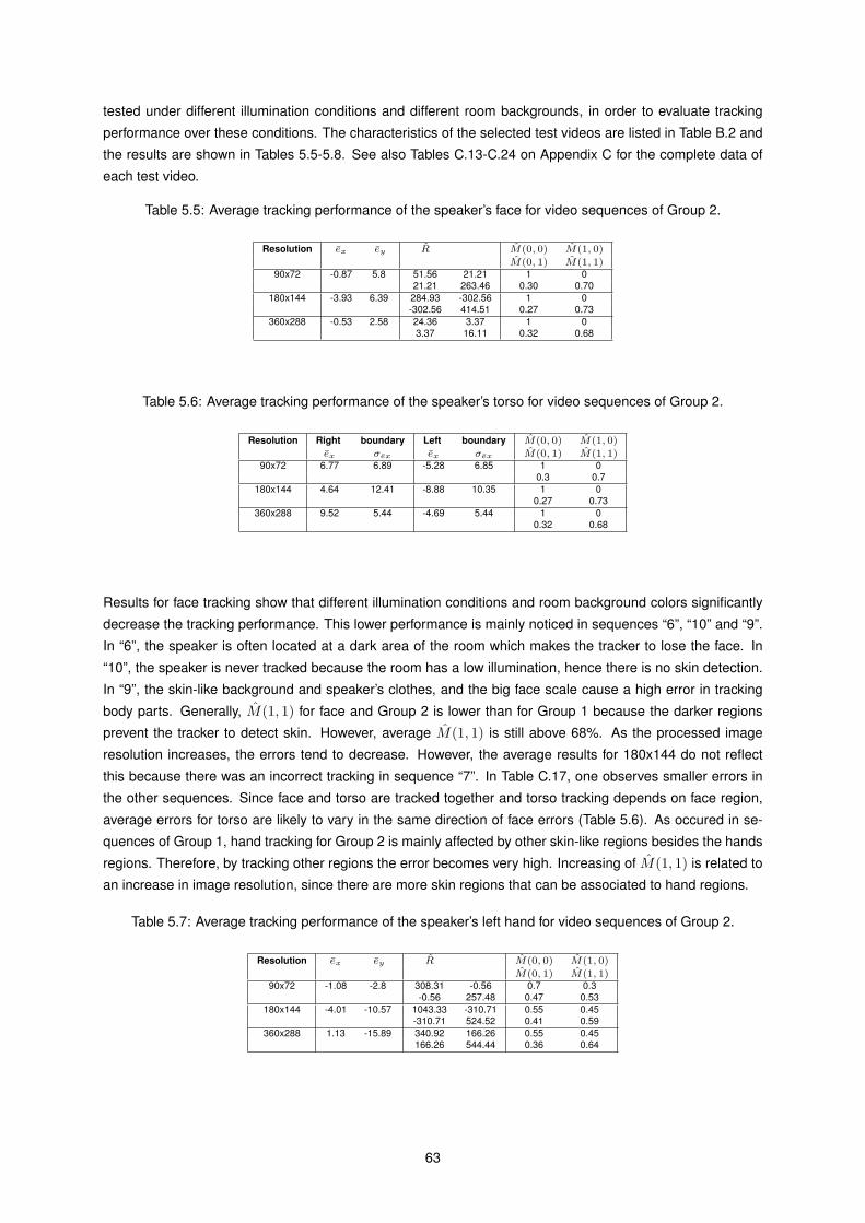
tested under different illumination conditions and different room backgrounds, in order to evaluate tracking
performance over these conditions. The characteristics of the selected test videos are listed in Table B.2 and
the results are shown in Tables 5.5-5.8. See also Tables C.13-C.24 on Appendix C for the complete data of
each test video.
Table 5.5: Average tracking performance of the speaker’s face for video sequences of Group 2.
Resolution ex ey R M(0, 0) M(1, 0)
M(0, 1) M(1, 1)90x72 -0.87 5.8 51.56 21.21 1 0
21.21 263.46 0.30 0.70180x144 -3.93 6.39 284.93 -302.56 1 0
-302.56 414.51 0.27 0.73360x288 -0.53 2.58 24.36 3.37 1 0
3.37 16.11 0.32 0.68
Table 5.6: Average tracking performance of the speaker’s torso for video sequences of Group 2.
Resolution Right boundary Left boundary M(0, 0) M(1, 0)
ex σex ex σex M(0, 1) M(1, 1)90x72 6.77 6.89 -5.28 6.85 1 0
0.3 0.7180x144 4.64 12.41 -8.88 10.35 1 0
0.27 0.73360x288 9.52 5.44 -4.69 5.44 1 0
0.32 0.68
Results for face tracking show that different illumination conditions and room background colors significantly
decrease the tracking performance. This lower performance is mainly noticed in sequences “6”, “10” and “9”.
In “6”, the speaker is often located at a dark area of the room which makes the tracker to lose the face. In
“10”, the speaker is never tracked because the room has a low illumination, hence there is no skin detection.
In “9”, the skin-like background and speaker’s clothes, and the big face scale cause a high error in tracking
body parts. Generally, M(1, 1) for face and Group 2 is lower than for Group 1 because the darker regions
prevent the tracker to detect skin. However, average M(1, 1) is still above 68%. As the processed image
resolution increases, the errors tend to decrease. However, the average results for 180x144 do not reflect
this because there was an incorrect tracking in sequence “7”. In Table C.17, one observes smaller errors in
the other sequences. Since face and torso are tracked together and torso tracking depends on face region,
average errors for torso are likely to vary in the same direction of face errors (Table 5.6). As occured in se-
quences of Group 1, hand tracking for Group 2 is mainly affected by other skin-like regions besides the hands
regions. Therefore, by tracking other regions the error becomes very high. Increasing of M(1, 1) is related to
an increase in image resolution, since there are more skin regions that can be associated to hand regions.
Table 5.7: Average tracking performance of the speaker’s left hand for video sequences of Group 2.
Resolution ex ey R M(0, 0) M(1, 0)
M(0, 1) M(1, 1)90x72 -1.08 -2.8 308.31 -0.56 0.7 0.3
-0.56 257.48 0.47 0.53180x144 -4.01 -10.57 1043.33 -310.71 0.55 0.45
-310.71 524.52 0.41 0.59360x288 1.13 -15.89 340.92 166.26 0.55 0.45
166.26 544.44 0.36 0.64
63

Table 5.8: Average tracking performance of the speaker’s right hand for video sequences of Group 2.
Resolution ex ey R M(0, 0) M(1, 0)
M(0, 1) M(1, 1)90x72 0.23 -0.74 188.01 -159.1 0.98 0.02
-159.1 466.52 0.5 0.5180x144 -2.13 -0.97 1010.8 -547.64 0.62 0.38
-547.64 1060.95 0.37 0.63360x288 10.07 -11.64 302.02 -108.64 0.82 0.18
-108.64 1057.78 0.38 0.62
5.4 Activity Recognition EvaluationThis section describes the metrics used to evaluate the activity classifiers and presents the experimental
results of their performance.
5.4.1 Recognition MetricsWhen evaluating a classifier performance, it is essential to measure its ability to correctly detect when an
activity occurs (true positive), but also measure the ability of not detecting an activity that did not occur (true
negative). Accordingly, true and false positives are measured through a confusion matrix, which relates clas-
sifications of the expert and the trained classifier. For each activity and test video sequence, a matrix must be
constructed.
A GT activity occurrence aGT is said to be correctly recognized, if there is an automatic detection a =[u−K + 1, v] (see Feature Vector in 4.3.1) whose overlap is at least O, ie:
#(a ∩ aGT )#(a ∪ aGT )
≥ O%. (5.7)
where O = 50. By requiring an overlap of 50% one ensures that a single detection a matches with each
activity aGT . Performance of each activity classifier is evaluated through a confusion matrix M , and classifier’s
precision and recall. Let M(o, p) be the probability that an activity a is estimated with label p, given the correct
label o. Precision measures classifier’s exactness, ie, the ability to detect only the activity occurrences. Recall
measures classifier completeness, ie, the ability to detect all the activity occurrences. Precision and recall are
given by (5.8) and (5.9), respectively.
Precision =TP
TP + FP(5.8)
Recall =TP
TP + FN(5.9)
In (5.8)-(5.9), TP is the true positives number, FP is the false positives number and FN is the false negatives
number. A match between aGT and a is a TP , a GT activity occurrence with no matching detections is a FN
and a detected activity that does not match GT is a FP .
5.4.2 Results of Activity ClassifiersAs mentioned in Section 4.3.1, to train an activity some parameters have to be defined. To test an activity,
these parameters are the same. In the following sections, the experimental results for each activity (A to F)
are presented. These experimental tests allow to compare different combinations of settings, and draw some
conclusions about them.
Since the system only starts collecting features once the background model is built, the activity occurrences
aGT before that initialization are not considered in the evaluation. In the graphics above, Prob. FP and Prob.
FN denote the probabilities of false positives and false negatives, taken from the confusion matrix M . The
64
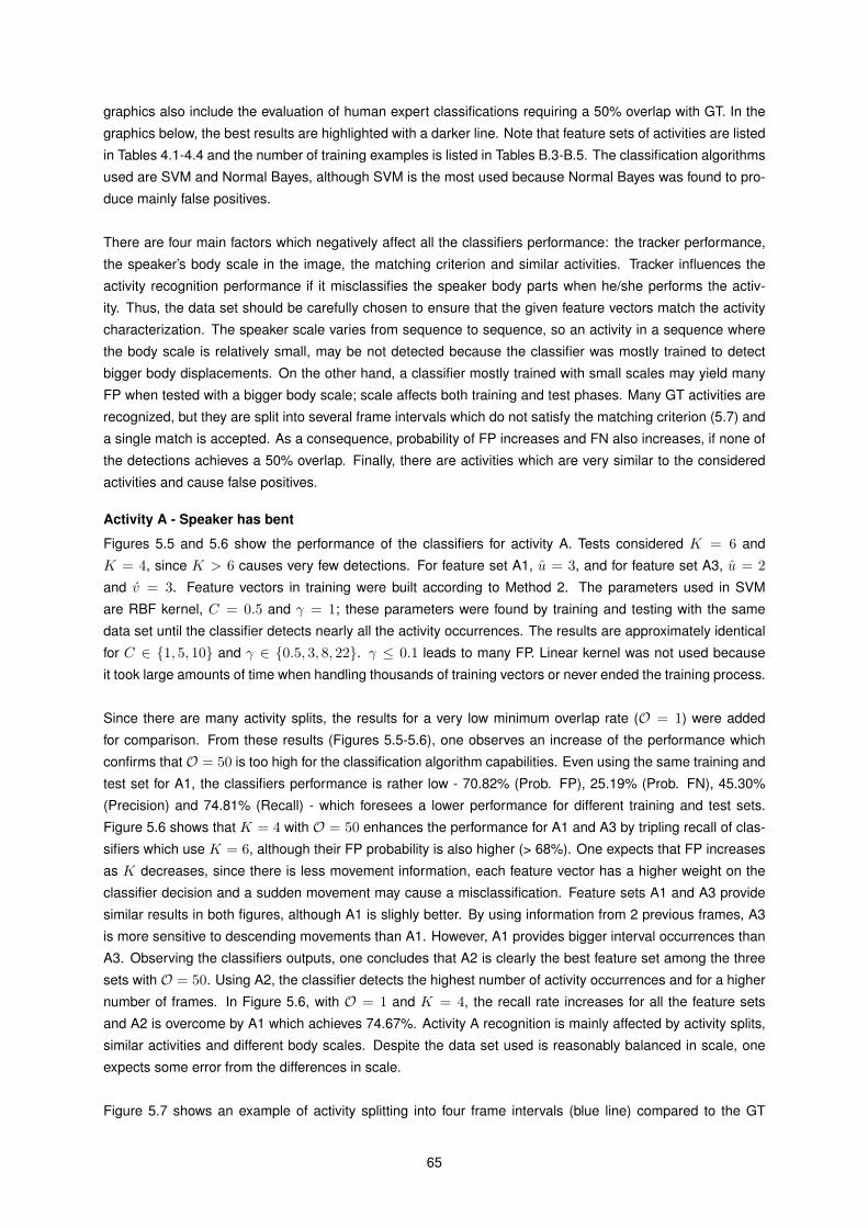
graphics also include the evaluation of human expert classifications requiring a 50% overlap with GT. In the
graphics below, the best results are highlighted with a darker line. Note that feature sets of activities are listed
in Tables 4.1-4.4 and the number of training examples is listed in Tables B.3-B.5. The classification algorithms
used are SVM and Normal Bayes, although SVM is the most used because Normal Bayes was found to pro-
duce mainly false positives.
There are four main factors which negatively affect all the classifiers performance: the tracker performance,
the speaker’s body scale in the image, the matching criterion and similar activities. Tracker influences the
activity recognition performance if it misclassifies the speaker body parts when he/she performs the activ-
ity. Thus, the data set should be carefully chosen to ensure that the given feature vectors match the activity
characterization. The speaker scale varies from sequence to sequence, so an activity in a sequence where
the body scale is relatively small, may be not detected because the classifier was mostly trained to detect
bigger body displacements. On the other hand, a classifier mostly trained with small scales may yield many
FP when tested with a bigger body scale; scale affects both training and test phases. Many GT activities are
recognized, but they are split into several frame intervals which do not satisfy the matching criterion (5.7) and
a single match is accepted. As a consequence, probability of FP increases and FN also increases, if none of
the detections achieves a 50% overlap. Finally, there are activities which are very similar to the considered
activities and cause false positives.
Activity A - Speaker has bent
Figures 5.5 and 5.6 show the performance of the classifiers for activity A. Tests considered K = 6 and
K = 4, since K > 6 causes very few detections. For feature set A1, u = 3, and for feature set A3, u = 2and v = 3. Feature vectors in training were built according to Method 2. The parameters used in SVM
are RBF kernel, C = 0.5 and γ = 1; these parameters were found by training and testing with the same
data set until the classifier detects nearly all the activity occurrences. The results are approximately identical
for C ∈ 1, 5, 10 and γ ∈ 0.5, 3, 8, 22. γ ≤ 0.1 leads to many FP. Linear kernel was not used because
it took large amounts of time when handling thousands of training vectors or never ended the training process.
Since there are many activity splits, the results for a very low minimum overlap rate (O = 1) were added
for comparison. From these results (Figures 5.5-5.6), one observes an increase of the performance which
confirms that O = 50 is too high for the classification algorithm capabilities. Even using the same training and
test set for A1, the classifiers performance is rather low - 70.82% (Prob. FP), 25.19% (Prob. FN), 45.30%
(Precision) and 74.81% (Recall) - which foresees a lower performance for different training and test sets.
Figure 5.6 shows that K = 4 with O = 50 enhances the performance for A1 and A3 by tripling recall of clas-
sifiers which use K = 6, although their FP probability is also higher (> 68%). One expects that FP increases
as K decreases, since there is less movement information, each feature vector has a higher weight on the
classifier decision and a sudden movement may cause a misclassification. Feature sets A1 and A3 provide
similar results in both figures, although A1 is slighly better. By using information from 2 previous frames, A3
is more sensitive to descending movements than A1. However, A1 provides bigger interval occurrences than
A3. Observing the classifiers outputs, one concludes that A2 is clearly the best feature set among the three
sets with O = 50. Using A2, the classifier detects the highest number of activity occurrences and for a higher
number of frames. In Figure 5.6, with O = 1 and K = 4, the recall rate increases for all the feature sets
and A2 is overcome by A1 which achieves 74.67%. Activity A recognition is mainly affected by activity splits,
similar activities and different body scales. Despite the data set used is reasonably balanced in scale, one
expects some error from the differences in scale.
Figure 5.7 shows an example of activity splitting into four frame intervals (blue line) compared to the GT
65

(a) Probability of error of the classifiers using SVM for each feature set.
(b) Precision and recall of the classifiers.
Figure 5.5: Performance of the classifiers for activity A (K = 6).
frame interval (green line). Classification values 1, -1 and -2 denote the activity detection, and 0 or no line
denotes no detection. Each automatic detection represents the occurrence of A in the previous K frames
and the orange line denotes the merged frame intervals where A occurred. In the example, since the activity
matching criterion is not verified, one FN is added and each estimated frame interval is accounted as FP.
This example shows why the FN and FP probabilities are high for O = 50, although the activities are partially
recognized.
Activity B - Speaker’s face is visible
Results of activity B are shown in Figure 5.8. Using Normal Bayes, the results are equal both for B1 and B2
and slightly better than B3. Main causes of errors in classification are false detections of the speaker (see an
example in Figure 5.9(a)) leading the classifier to detect activity B; and GT activities which are split because
the tracker has lost the speaker, leading to a false positive increase (Figures 5.9(b)-5.9(c) and 5.10(a)). From
the presented results, one concludes that the feature sets tested appear to be equally valid for recognizing B.
The classifiers performance is highly affected by tracking performance, so an improvement on tracking would
set precision and recall to nearly 100% as already occurs for many sequences of the dataset (see an example
in Figure 5.10(b)).
The parameters used in SVM are RBF kernel, C = 10 and γ = 8.0. Using SVM as classification algo-
rithm, the classifiers performance is lower than the Bayes-based classifiers. As well as the Bayes classifiers,
SVM-based classifiers have shown to split one activity into several activities, but also to always detect B for
one of the test set. This may be caused by giving negative examples labeled as positive when the tracker
loses the speaker in training for a while. Since SVM separates data using a hyperplane, negative examples
66
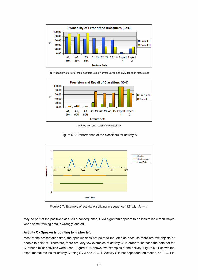
(a) Probability of error of the classifiers using Normal Bayes and SVM for each feature set.
(b) Precision and recall of the classifiers
Figure 5.6: Performance of the classifiers for activity A
Figure 5.7: Example of activity A splitting in sequence “12” with K = 4.
may be part of the positive class. As a consequence, SVM algorithm appears to be less reliable than Bayes
when some training data is wrongly labeled.
Activity C - Speaker is pointing to his/her left
Most of the presentation time, the speaker does not point to the left side because there are few objects or
people to point at. Therefore, there are very few examples of activity C. In order to increase the data set for
C, other similar activities were used. Figure 4.14 shows two examples of the activity. Figure 5.11 shows the
experimental results for activity C using SVM and K = 1. Activity C is not dependent on motion, so K = 1 is
67

(a) Probability of error of the classifiers using Normal Bayes and SVM for each feature set.
(b) Precision and recall of the classifiers
Figure 5.8: Performance of the classifiers for activity B
(a) Person is tracked in 2 frames, al-though the face is not considered tobe visible. This face detection causesa false positive in the activity B classi-fication.
(b) In frame 532 speaker is beingtracked and the classifier detects ac-tivity B.
(c) In frame 533 the tracker loses thespeaker and the classifier stops rec-ognizing B, causing a split in the ac-tivity.
Figure 5.9: Examples of error causes in recognizing activity B.
enough to recognize C. Nevertheless, experimental tests have shown an increase of activity splits for K > 1,
leading to a higher FP probability and poorer results. The parameters used in SVM are equal to activity A.
Results show that the best feature set is C5 which achieves 65% of recall and 32.5% of precision forO = 50%(see Figure 5.11). When requiring at least 1% overlap, C5 is overcome by C3 whose recall and precision
achieve 90% and 44.71%, respectively. Although C2, C3 and C5 provide a recognition of 90% of the activities
for O = 1%, C3 is considered the best, since it outputs less FP in both overlap rates (41.2% and 15.55%).
This shows that features of C3 and C5 are useful to recognize most of the activity occurrences, but the clas-
sifiers also suffer from the activity splitting problem, as well as activity A classifiers. On the other hand, face’s
and left hand’s area used included in C4 are not useful to recognize C as shown in Figure 5.11 by the lower
performance of the classifier that uses C4. Some activity detections are similar to C and cause false positives
68

(a) Example of activity B splitting in sequence “26”.
(b) Example of activity B recognition in sequence “21”.
Figure 5.10: Examples of activity B estimations.
(see Figure5.12(a)) and other FP are caused by errors in hand tracking (Figure 5.12(b)).
Figure 5.13 shows two examples of estimations of C. In Figure 5.13(a), the GT activity in frame interval
[1099, 1157] was split into intervals [1094, 1099], [1102, 1102], [1128, 1141] and [1154, 1155]. The activity
split in C is mainly caused by the tracking algorithm which temporarily loses the left hand location. Although C
has been recognized, none of the frame intervals satisfies (5.7), hence four FP and one FN were considered.
In Figure 5.13(b) the GT activity ([663, 692]) was split into [660, 669] and [674, 694] where the hand tracking
is also affecting the activity recognition module. Note also that in Figure 5.13(b), the classifier estimates C in
the frames before and after the GT interval because the speaker is performing a similar activity to C as shown
in Figure 5.14.
Activity D - Speaker is pointing to his/her right
Classifiers of activity D were trained with the same SVM parameters used to train activities A and C. Per-
formance of activity D classifiers is significantly lower than C classifiers (see Figure 5.15). The differences
in performance are explained by the different data set which was even more carefully chosen for activity C.
Ideally, one should ensure that the tracker is able to track correctly the right hand in every training example,
in order to provide correct features. However, activity D data set is bigger and it is hard to guarantee a correct
tracking for all the examples. These results clearly show how the training examples and the tracker perfor-
mance may affect the classifiers performance.
In Figure 5.15, D4 (analogous to C4) still provides the worst detection rates. With O = 50, precision and
recall are similar for D1, D2, D3 and D5, although D3 is slightly better. With O = 1, D5 and D3 confirm their
higher quality (compare with results of C5 and C3 in Figure 5.11) and D3 still provides less FP than D5. Note
69

(a) Probability of error of the classifiers using SVM for each feature set.
(b) Precision and recall of the classifiers.
Figure 5.11: Performance of the classifiers for activity C
(a) Activity very similar to C in frame1097 of sequence “33”.
(b) FP in frame 961 of sequence “39”.Face and left hand belong to the sameskin blob, so another skin-like objectwas assigned to LH.
Figure 5.12: Examples of FP of activity C.
that the high amount of splits of each occurrence causes a probability of FP above 49.5% for O ∈ 1, 50. In
sum, D3 and D5 provide the best performance and D4 provides the lowest performance. Such as described
for activity C, similar activities to D and tracking errors also lead to an increase of FP. In sequences “44” to
“57”, the speaker is not tracked for some seconds because the BS algorithm is not able to detect speaker’s
foreground pixels, since the strong white illumination makes the speaker’s shirt color similar to the background
color. Consequently, there are wrong features which result in a partially incorrect training and test. Figure
5.16 shows three examples of estimations of D. The activity split into four parts in Figure 5.16(a) confirms
hand tracking as a critical task to recognize D (see also Figure 5.13(a)). Figure 5.16(b) shows the detection
of a similar activity in [818, 822] (see Figure 5.17) and an interval which is very close to the GT.
Activity E - Speaker has moved to his/her left
Classifiers performance is shown in Figure 5.18. Classifiers were trained and tested with SVM, K = 11 and
Method 1 for building training vectors. K value was given by the frame number of the smallest training exam-
70
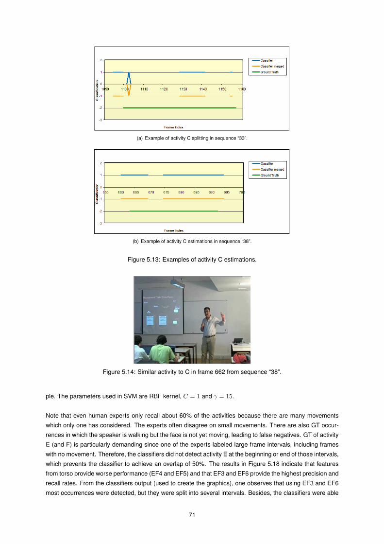
(a) Example of activity C splitting in sequence “33”.
(b) Example of activity C estimations in sequence “38”.
Figure 5.13: Examples of activity C estimations.
Figure 5.14: Similar activity to C in frame 662 from sequence “38”.
ple. The parameters used in SVM are RBF kernel, C = 1 and γ = 15.
Note that even human experts only recall about 60% of the activities because there are many movements
which only one has considered. The experts often disagree on small movements. There are also GT occur-
rences in which the speaker is walking but the face is not yet moving, leading to false negatives. GT of activity
E (and F) is particularly demanding since one of the experts labeled large frame intervals, including frames
with no movement. Therefore, the classifiers did not detect activity E at the beginning or end of those intervals,
which prevents the classifier to achieve an overlap of 50%. The results in Figure 5.18 indicate that features
from torso provide worse performance (EF4 and EF5) and that EF3 and EF6 provide the highest precision and
recall rates. From the classifiers output (used to create the graphics), one observes that using EF3 and EF6
most occurrences were detected, but they were split into several intervals. Besides, the classifiers were able
71

(a) Probability of error of the classifiers using SVM for each feature set.
(b) Precision and recall of the classifiers.
Figure 5.15: Performance of the classifiers for activity D
to detect even smaller movements to the left, which also produces an increase of FP. By using information
about three previous frames in EF6, its classifier provides more detections of the same GT occurrence than
EF3 which uses only two previous frames. However, classifiers that use EF3 provide slightly better results
than classifiers with EF6 (Figure 5.18). From the classifiers output, one observes that feature sets EF1 and
EF2 provide less FP because their classifiers detect less activity splits than the other sets. Therefore, they
have more difficulty satisfying the matching condition and they are worse than EF3 and EF6.
Figure 5.19 shows two examples of activity splitting where each activity was split into four and two inter-
vals, respectively. In these examples it is clear that a 50% overlap is not achieved although the activities have
been recognized. After evaluating these classifiers, it was found that Method 2 for feature vectors was better
than Method 1 because it creates much more feature vectors from the same activity example, providing a
higher data set. By using Method 2, one expects a decrease in FN and a high number of FP caused by the
activity splits.
Although the performance is low for O = 50 (29.02% recall with E3), the current results are promising since
recall is already high for O = 1 (86.23%). Recall may be increased with Method 2 and precision may be
improved by using another classification algorithm which produces less splits. It is important to refer that the
activity recognition is performed in a very low image resolution, and yet the classifiers are able to recognize
small movements to the left.
Activity F - Speaker has moved to his/her right
Figure 5.20 presents the results of activity F with K = 11. The parameters used in SVM are equal to activity
E. Classifiers of activities E and F only differ on the data set. For O = 50, EF1 provides the highest recall and
precision (14.94% and 19.04% respectively), although they are still low. As presented for activity E, EF3 and
EF6 still remain as the top feature sets, and EF2, EF4 and EF5 provide the lowest performance. For O = 1,
the results confirm EF3 and EF6 as the best feature sets (compare with results shown in Figure 5.18). Using
72

(a) Example of activity D splitting in sequence “48”.
(b) Examples of correct estimation of D and similar activity (sequence “44”).
Figure 5.16: Examples of activity D estimations.
Figure 5.17: Similar activity to D in frame 818 from sequence “44”.
EF3 and EF6, the classifiers achieve recall rates of 61.44% and 52.02% respectively.
In Figure 5.20(a), one observes that Expert 2 does not consider 70.40% of the activities, while Expert 1
only misses 2.21%. This shows that there was a significantly different criteria when labeling the activities.
As a result, by setting Th = 1, the GT of F has been heavily affected by Expert 1 criteria. To avoid this
situation, GT should have been defined by the frame intervals where several experts agree on the activity
occurrence as discussed below in Section 5.6. In Figure 5.18 the experts’ recall is reasonably balanced while
in activity F, Expert 1 has three times the recall of Expert 2. The difference between the two experts shows
that there is a large amount of occurrences which are not easily identified or/and the experts have different
labeling criteria. As described for the previous activities and particurlarly for E, activity F occurrences were
also split into several parts. Note that in Figure 5.21 the overlap between the green and orange lines is 44%
and 73.9%, but according to the evaluation method none of these estimations was accounted as a true pos-
73

(a) Probability of error of the classifiers using SVM for each feature set.
(b) Precision and recall of the classifiers.
Figure 5.18: Performance of the classifiers for activity E
itive. Since the training is not as rigorous as the expert, the classifiers are not able to recognize as much as
Expert 1. This very demanding GT is the main reason why the performance of F’s classifiers is even lower
than E’s classifiers. On the other hand, the use of Method 1 instead of Method 2 also affects the performance.
Nevertheless, the best classifier achieved 61.44% (recall) and 46.85% (precision) with O = 1, which denotes
significant results given the GT.
Best Results of Classifiers
Table 5.9 presents the best results of each classifier according to (5.7). Since activities C and D are analogous
and the classifier of C achieved a 65% recall, the classifier of D may also achieve better results by performing
a better labeling and improving hand tracking to avoid FP as shown in Figure 5.12(b). For E and F, there is
still room for improvements by using another method for creating the feature vectors (Method 2).
Generally, the classifiers have correctly detected a high number of activity occurrences, but most of the
Table 5.9: Best results for each activity classifier. FP Prob. is the false positive probability and FN Prob. isthe false negative probability. A to F identify the activities.
Rates (%) / Activity A B C D E FFP Prob. 76.08 10.00 43.61 72.13 81.15 35.70FN Prob. 90.00 13.33 35.00 85.57 70.98 85.06Precision 2.39 86.67 32.50 2.44 6.41 19.04
Recall 10.00 86.67 65.00 14.43 29.02 14.94
occurrences were detected in several small frame intervals (see Figures 5.5-5.20 with O = 1). Therefore,
74
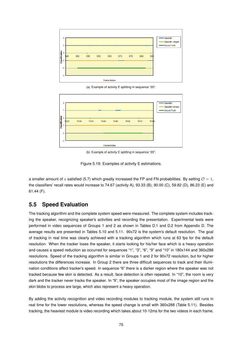
(a) Example of activity E splitting in sequence “20”.
(b) Example of activity E splitting in sequence “20”.
Figure 5.19: Examples of activity E estimations.
a smaller amount of a satisfied (5.7) which greatly increased the FP and FN probabilities. By setting O = 1,
the classifiers’ recall rates would increase to 74.67 (activity A), 93.33 (B), 90.00 (C), 59.82 (D), 86.23 (E) and
61.44 (F).
5.5 Speed EvaluationThe tracking algorithm and the complete system speed were measured. The complete system includes track-
ing the speaker, recognizing speaker’s activities and recording the presentation. Experimental tests were
performed in video sequences of Groups 1 and 2 as shown in Tables D.1 and D.2 from Appendix D. The
average results are presented in Tables 5.10 and 5.11. 90x72 is the system’s default resolution. The goal
of tracking in real time was clearly achieved with a tracking algorithm which runs at 63 fps for the default
resolution. When the tracker loses the speaker, it starts looking for his/her face which is a heavy operation
and causes a speed reduction as occurred for sequences “1”, “3”, “6”, “9” and “10” in 180x144 and 360x288
resolutions. Speed of the tracking algorithm is similar in Groups 1 and 2 for 90x72 resolution, but for higher
resolutions the differences increase. In Group 2 there are three difficult sequences to track and their illumi-
nation conditions affect tracker’s speed. In sequence “6” there is a darker region where the speaker was not
tracked because few skin is detected. As a result, face detection is often repeated. In “10”, the room is very
dark and the tracker never tracks the speaker. In “9”, the speaker occupies most of the image region and the
skin blobs to process are large, which also represent a heavy operation.
By adding the activity recognition and video recording modules to tracking module, the system still runs in
real time for the lower resolutions, whereas the speed change is small with 360x288 (Table 5.11). Besides
tracking, the heaviest module is video recording which takes about 10-12ms for the two videos in each frame.
75

(a) Probability of error of the classifiers using SVM for each feature set.
(b) Precision and recall of the classifiers.
Figure 5.20: Performance of the classifiers for activity F
(a) Example of activity F splitting in sequence “27”.
(b) Example of activity F splitting in sequence “19”.
Figure 5.21: Examples of activity F estimations.
Activity recognition module includes six activities and takes about 4-6ms for each frame. Processing in 90x72,
the speed reduction is higher because all the videos are recorded in the original body scale. Tests were per-
76

formed on a Pentium IV at 2.66 GHz with 1GB of memory.
Table 5.10: Tracker’s average speed for three image resolutions.
Data Resolution/fpsset 90x72 180x144 360x288
Group 1 63.02 50.64 22.23Group 2 63.15 43.58 19.88
Table 5.11: System’s average speed over three image resolutions (tracking, video recording and activityrecognition).
Data Resolution/fpsset 90x72 180x144 360x288
Group 1 43.37 33.54 19.57Group 2 43.32 32.48 17.32
5.6 DiscussionGenerally, performance of face and torso tracking is quite acceptable for an activity recognition system, given
the results achieved (see Section 5.4.2). When the tracker correctly finds these body part locations, the errors
are mostly low for every image resolution as shown in Tables 5.1-5.2 which denotes a satisfactory face and
torso tracking. On the other hand, the speaker presence when the background model is being built, produces
very few foreground pixels and causes no speaker detections in some cases. Therefore, the tracking algo-
rithm requires the scene without the speaker when the background model is being initialized. Provided that
no reliable face detector was available for a small face scale, and the algorithm requires a square skin blob
(see Section 4.2.2), the tracker takes some time to detect the speaker (mostly < 25 frames). Note that the 50
samples randomly chosen do not provide a thorough evaluation of the tracker. Instead, they allow to obtain
an overview on the tracking performance.
Moreover, the presentation rooms contain many skin-like regions (objects and audience) which breaks one
of the algorithm’s assumptions. Therefore, hand tracking algorithm has a large amount of skin-like regions
to handle, without no hand detector that would be useful for a robust detection. Micilotta et al. [Mici 05] that
used a trained hand detector confirm the difficulty of creating a reliable hand detector when compared with
the other body part detectors. They justify their detector’s lower performance with the high variability of hand
shape which was also noticed in this work. Although the average detection rate for hands is between 52%
and 83%, in sequence “1” the detection rate achieved 80% and 92% for left and right hands without hand
detectors (Tables C.3-C.4). Therefore, the hand tracking algorithm has shown to be reliable whenever there
are few or no other skin-like regions. A difficulty which affects the tracker is the face and hand(s) in the same
skin blob. This situation may cause the tracker to lose the face or the hand, or even to assign the speaker’s
hand to F (t). Besides, it increases the average error of face and hand tracking.
In activity recognition, the activity splits are the main cause of low performance for O = 50, as well as
the number of small frame intervals of each split. GT of activities E and F is hard to achieve by an auto-
matic classifier because many labeled frame intervals are larger than the real movement interval. Besides,
when the speaker turns his/her face, Fx changes gradually and some FP of E or F are detected. In most
activity classifiers, similar activities are a relevant cause of FP and show classifiers sensitivity and ability to
77
recognize their specific type of activity. In previous experimental tests, Normal Bayes has been found to be
very imprecise and was not used for most of the activity classifiers. In these tests, Bayes-based classifiers
presented higher recall rates than SVM, but they relied on a very high number of detections that led to a low
precision. The classifiers performance would be improved by creating all the feature vectors with Method 2
and rejecting Method 1; considering most experts opinions by setting Th = max(2, E − 1); and using as
automatic activity estimations (a) the frame intervals obtained by merging the intervals where the activities
occurred, ie, the frame intervals in orange exemplified in Figures 5.7-5.21. A more comprehensive test on the
SVM parameters would provide information about whether there is a set of parameters that simultaneously
reduces activity splits and increases the occurrences interval. This test should be performed with the same
training and test data, since it produces the best case performance.
The speed measurements show that the algorithms used are suitable for a real-time system (Tables 5.10-
5.11). Considering that the current hardware is quite faster than the test machine, by using it one expects a
real-time performance for 360x288 resolution.
5.7 ConclusionsExperimental tests have shown promising results. The tracking algorithm is able to track the speaker without
body part detectors and provides both frontal and side tracking as well as body scale adaptation. Besides, it
shows low dependency on the BS performance. The tracker produces low estimation errors when there are
no skin-like regions besides the speaker, and when the room illumination allows an effective skin detection. It
is also tolerant to speaker’s slow or fast movements and to camera’s slow movements.
In activity recognition, the classifiers were successful, detecting the majority of the activities, although there
are still many activity splits. The high number of correct activity detections is remarkable, provided that recog-
nition is achieved with a very low image resolution (90x72).
The proposed system is quite fast and performs in real time for lower resolutions (> 32.48 fps). Therefore,
the system still allows an addition of several new activities or other features.
78
Chapter 6
Conclusions
6.1 Work ReviewInteractive presentations are a very significant way of sharing knowledge between people. Nowadays, trans-
mitting effectively a complex idea to others may require technological advanced tools, such as virtual tables
and other specialized software, although most of them simply rely on slide shows. Moreover, remote real-time
presentations are even more demanding as they require sharing and synchronizing all the presentation re-
sources among all the participants.
Nearly all of the presentation participants are still unaware of the existing interactions between them and how
often they occur. By evaluating the interactions and behaviors from movements, the speaker(s) or the other
participants may perceive their flaws and improve their communication strategy. Since each presentation is
unique due to speaker’s state of mind and different audience, one may desire to preserve that information on
video and audio with low cost and effort, for later viewing or sharing.
Increasing of the tracking systems’ robustness over the years has enabled focusing on human activity recogni-
tion from video and audio. Activity recognition systems present many applications both for presentations and
meetings, video surveillance, automatic collection of statistics in sports or even to label videos by their content.
This dissertation presents a real-time system for human activity recognition and video recording, applied to
the interactive presentation environment. The developed system includes a human tracking algorithm for face,
torso and hands, an activity recognition module and a video recording module. This system has shown to be
able to track the presentation speaker under different illumination conditions, continuously adapt to speaker’s
scale, ignore most of the audience movements and track the speaker in both frontal and side views. More-
over, the system recognizes speaker’s activities and records the presentation in video, including a clipped
video which shows the speaker.
The identified goals for this thesis were generally accomplished. The detection probability of the speaker
achieves 76% with the default resolution and 85% with the original resolution. Hand tracking is above 52%
and it is considered an important achievement, given the amount of skin-like regions around the speaker. The
presented results for activity recognition are mostly below the defined values of success criteria. However, it
was shown that the classifiers, in fact, recognize a high number of activity occurrences. Most of the activities
were split by the classifiers and it results on a lower performance, according to the evaluation criterion. Still,
the proposed system presents a solid basis for further development.
79

6.2 Future WorkFuture research should mainly focus on human tracking and activity recognition. Human tracking involves
some hard issues to handle, given the scene conditions. Partial occlusion situations and body part detection
deserve some improvements. In activity recognition there is still room for experiments which may improve
classifiers performance. Therefore, main issues for future work are the following:
• Enhance face and hand detection robustness. By training face and hand detectors with the pre-
sentation images, the tracker performance would increase and the system would be less depend on
illumination and room background. Using body part detectors decreases/eliminates the need of a seg-
mentation algorithm, and the system would start recognizing activities once the presentation starts
without initialization.
• Experiment new training/test parameters. The best feature sets of each activity should be tested
with new sliding window sizes and Method 2 for feature vectors. For E and F, recommended K are 7,
9, 13 and 15. For activity A, K is 2 and 3.
• Add new classification algorithms. Since SVM produce many splits and Normal Bayes yields many
false positives, one should consider other classification algorithms which may achieve better results.
Still, SVM parameters deserve a comprehensive testing.
• Perform experiments on a single body scale. Training classifiers with different body scales led to
a considerable amount of false positives and false negatives. Only after we have obtained the best
classifier parameters for the same scale, we are ready to experiment on different scales.
• Train activity classifiers in higher resolutions. Using higher image resolutions there is more infor-
mation about the speaker movements and this information may be used to recognize small movements
that the lower resolutions ignore.
• Train activity classifiers with alternate frames. In slow movements, features of consecutive frames
are nearly equal, and jumping some frames may help recognizing them, while speeding up the system.
Furthermore, jumping frames will provide information about how classifiers performance is affected.
• Add new activities. List of recognized activities should be extended taking into account the needs of
the system user. Adding new activities is easy and fast. After improving the classifier of activity A, its
parameters may be used to recognize when the speaker rises (A2). By adding an activity component
equal to A and providing the correct activity examples, a classifier for A2 is ready to use. Other activities
may be a hand pointing down, a hand above the face or “the speaker has not moved for t seconds”.
80

Bibliography
[Adle 07] M. Adler and F. Reynolds. “Vision-Guided "Point and Click" for Smart Rooms”. In: ICSNC ’07:
Proceedings of the Second International Conference on Systems and Networks Communications,
p. 30, IEEE Computer Society, Washington, DC, USA, 2007.
[Al H 05] M. Al-Hames, A. Dielmann, D. Gatica-Perez, S. Reiter, S. Renals, and D. Zhang. “Multimodal Inte-
gration for Meeting Group Action Segmentation and Recognition”. IDIAP-RR 31, IDIAP, Martigny,
Switzerland, 2005. Published in “MLMI”, July, 2005.
[Al H 07] M. Al-Hames, C. Lenz, S. Reiter, J. Schenk, F. Wallhoff, and G. Rigoll. “Robust Multi-Modal Group
Action Recognition in Meetings from Disturbed Videos with the Asynchronous Hidden Markov
Model.”. In: ICIP (2), pp. 213–216, IEEE, 2007.
[Arts 09] eHow Arts and E. Editor. “How to Keep Face and Hand Proportions Realis-
tic When Drawing the Human Form”. 2009. www.ehow.com/how_2213390_
keep-face-hand-proportions-realistic.html Last access on: June 10th, 2009.
[Baud 93] T. Baudel and M. Beaudouin-lafon. “CHARADE: Remote Control of Objects Using Free-Hand
Gestures”. Communications of the ACM, Vol. 36, pp. 28–35, 1993.
[Bern 06] K. Bernardin, H. K. Ekenel, and R. Stiefelhagen. “Multimodal Identity Tracking in a Smartroom”.
In: AIAI, pp. 324–336, 2006.
[Bhat 02] S. Bhattacharya. “Intelligent monitoring systems: smart room for patient’s suffering from som-
nambulism”. In: Microtechnologies in Medicine and Biology 2nd Annual International IEEE-EMB
Special Topic Conference on, pp. 326–331, 2002.
[Bobi 01] A. F. Bobick, J. W. Davis, I. C. Society, and I. C. Society. “The Recognition of Human Movement
Using Temporal Templates”. IEEE Transactions on Pattern Analysis and Machine Intelligence,
Vol. 23, pp. 257–267, 2001.
[Brad 98] G. R. Bradski. “Computer Vision Face Tracking For Use in a Perceptual User Interface”. 1998.
[Bran 00] M. Brand and V. Kettnaker. “Discovery and Segmentation of Activities in Video”. PAMI, Vol. 22,
No. 8, pp. 844–851, August 2000.
[Brem 06] F. Bremond, M. Thonnat, and M. Zuniga. “Video Understanding Framework For Automatic Behav-
ior Recognition”. Behavior Research Methods, Vol. 3, No. 38, pp. 416–426, 2006.
[Brox 03] T. Brox, M. Rousson, R. Deriche, and J. Weickert. “Unsupervised segmentation incorporating
colour, texture, and motion”. In: Computer Analysis of Images and Patterns, volume 2756 of
Lecture Notes in Computer Science, pp. 353–360, Springer, 2003.
[Burg 98] C. J. Burges. “A Tutorial on Support Vector Machines for Pattern Recognition”. Data Mining and
Knowledge Discovery, Vol. 2, pp. 121–167, 1998.
81
[Buss 05] C. Busso, S. Hernanz, C. wei Chu, S. il Kwon, S. Lee, P. G. Georgiou, I. Cohen, and S. Narayanan.
“Smart room: Participant and speaker localization and identification”. In: Proc. IEEE Int. Conf. on
Acoustics, Speech and Signal Processing (ICASSP), 2005.
[Cann 86] J. Canny. “A computational approach to edge detection”. IEEE Trans. Pattern Anal. Mach. Intell.,
Vol. 8, No. 6, pp. 679–698, November 1986.
[Cao 05] X. Cao, E. Ofek, and D. Vronay. “Evaluation of alternative presentation control techniques”. In:
CHI ’05: CHI ’05 extended abstracts on Human factors in computing systems, pp. 1248–1251,
ACM, New York, NY, USA, 2005.
[Chiu 03] P. Chiu, Q. Liu, J. S. Boreczky, J. Foote, D. Kimber, S. Lertsithichai, and C. Liao. “Manipulating
and Annotating Slides in a Multi-Display Environment.”. In: M. Rauterberg, M. Menozzi, and
J. Wesson, Eds., INTERACT, IOS Press, 2003.
[Chun 08] S. Chun, K. Hong, and K. Jung. “3D Star Skeleton for Fast Human Posture Representation”. In:
Proceedings of World Academy of Science, Engineering and Technology, pp. 273–282, October
2008.
[Coll 00] R. Collins, A. Lipton, T. Kanade, H. Fujiyoshi, D. Duggins, Y. Tsin, D. Tolliver, N. Enomoto, and
O. Hasegawa. “A System for Video Surveillance and Monitoring”. Tech. Rep. CMU-RI-TR-00-12,
Robotics Institute, Pittsburgh, PA, May 2000.
[Coma 00] D. Comaniciu, V. Ramesh, and P. Meer. “IEEE CVPR 2000 Real-Time Tracking of Non-Rigid
Objects using Mean Shift”. 2000.
[Coma 01] D. Comaniciu, V. Ramesh, and P. Meer. “The variable bandwidth mean shift and data-driven scale
selection”. In: Proc. 8th Intl. Conf. on Computer Vision, pp. 438–445, 2001.
[Coma 02] D. Comaniciu and P. Meer. “Mean shift: a robust approach toward feature space analysis”. Pattern
Analysis and Machine Intelligence, IEEE Transactions on, Vol. 24, No. 5, pp. 603–619, 2002.
[Cort 95] C. Cortes and V. Vapnik. “Support-Vector Networks”. Machine Learning, Vol. 20, pp. 273–297,
1995.
[D 07] P. R. P. V. G. D., K. S. Rao, and S. Yarramalle. “Unsupervised Image Segmentation Method based
on Finite Generalized Gaussian Distribution with EM and K-Means Algorithm”. In: International
Journal of Computer Science and Network Security, 2007.
[Datt 02] A. Datta, M. Shah, N. Da, and V. Lobo. “Person-on-Person Violence Detection in Video Data”. In:
IEEE International Conference on Pattern Recognition, 2002.
[Dese 03] T. Deselaers, D. Keysers, and H. Ney. “Clustering Visually Similar Images to Improve Image
Search Engines”. In: Informatiktage der Gesellschaft f"ur Informatik, p. 302, Bad Schussenried,
Germany, Nov. 2003.
[Desh 05] K. Deshmukhand and G. Shinde. “An Adaptive Color Image Segmentation”. ELCVIA, Vol. 5,
No. 4, pp. 12–23, 2005.
[Dist 09] M. I. S. District. 2009. www.mansfieldisd.org/timberview/staff/davimy/
documents/humanproportionshandout.doc Last access on: June 10th, 2009.
[Efro 03] A. A. Efros, E. C. Berg, G. Mori, and J. Malik. “Recognizing action at a distance”. In: ICCV,
pp. 726–733, 2003.
82
[Eken 07] H. Ekenel, M. Fischer, Q. Jin, and R. Stiefelhagen. “Multi-modal Person Identification in a Smart
Environment”. In: Biometrics07, pp. 1–8, 2007.
[Elga 00] A. Elgammal, D. Harwood, and L. Davis. “Non-parametric model for background subtraction”. In:
FRAME-RATE Workshop, IEEE, pp. 751–767, 2000.
[Felz 04] P. F. Felzenszwalb and D. P. Huttenlocher. “Efficient graph-based image segmentation”. Interna-
tional Journal of Computer Vision, Vol. 59, No. 2, 2004.
[Fock 02] D. Focken and R. Stiefelhagen. “Towards Vision-based 3-D People Tracking in a Smart Room”.
In: Multimodal Interfaces, 2002. Proceedings. Fourth IEEE International Conference on, pp. 400–
405, 2002.
[Fors 02] D. A. Forsyth and J. Ponce. Computer Vision: A Modern Approach. Prentice Hall, August 2002.
[Fuji 98] H. Fujiyoshi and A. J. Lipton. “Real-Time Human Motion Analysis by Image Skeletonization”. In:
Proceedings of IEEE WACV98, pp. 15–21, 1998.
[Fuku 75] K. Fukunaga and L. Hostetler. “The estimation of the gradient of a density function, with applica-
tions in pattern recognition”. Information Theory, IEEE Transactions on, Vol. 21, No. 1, pp. 32–40,
1975.
[Gela 06] E. D. Gelasca, T. Ebrahimi, M. Karaman, and T. Sikora. “A Framework for Evaluating Video Object
Segmentation Algorithms”. Computer Vision and Pattern Recognition Workshop, Vol. 0, p. 198,
2006.
[Gome 02] G. Gomez and E. F. Morales. “Automatic Feature Construction and a Simple Rule Induction Algo-
rithm for Skin Detection”. In: In Proc. of the ICML Workshop on Machine Learning in Computer
Vision, pp. 31–38, 2002.
[Hard 01] C. von Hardenberg and F. Bérard. “Bare-hand human-computer interaction”. In: PUI ’01: Pro-
ceedings of the 2001 workshop on Perceptive user interfaces, pp. 1–8, ACM, New York, NY, USA,
2001.
[Hari 00] I. Haritaoglu, D. Harwood, and L. S. David. “W4: Real-Time Surveillance of People and Their
Activities”. IEEE Trans. Pattern Anal. Mach. Intell., Vol. 22, No. 8, pp. 809–830, August 2000.
[Hass 08] R. Hassanpour, A. Shahbahrami, and S. Wong. “Adaptive Gaussian Mixture Model for Skin Color
Segmentation”. In: Proceedings of World Academy of Science, Engineering and Technology,
pp. 1–6, July 2008.
[Heik 99] J. Heikkilä and O. Silvén. “A real-time system for monitoring of cyclists and pedestrians”. In:
Second IEEE Workshop on Visual Surveillance, pp. 74–81, 1999.
[Heis 07] B. Heisele, T. Serre, and T. Poggio. “A Component-based Framework for Face Detection and
Identification”. International Journal of Computer Vision, Vol. 74, No. 2, pp. 167–181, August
2007.
[Henr 03] T. C. C. Henry, E. G. R. Janapriya, and L. C. de Silva. “An automatic system for multiple hu-
man tracking and actions recognition in office environment”. In: Proc. IEEE Int. Conf. Acoustics,
Speech, Signal Processing (ICASSP ’03), pp. 45–48, April 2003.
[Horp 00] T. Horprasert, D. Harwood, and L. S. Davis. “A robust background subtraction and shadow detec-
tion”. In: Proceedings of the Asian Conference on Computer Vision, pp. 983–988, 2000.
83

[Horp 99] T. Horprasert, D. Harwood, and L. S. Davis. “A Statistical Approach for Real-time Robust Back-
ground Subtraction and Shadow Detection”. In: ICCV Frame-Rate WS, 1999.
[Hurl 09] C. Hurley, S. Chen, J. Karim, and Google. “YouTube”. 2009. www.youtube.com Last access
on: June 10th, 2009.
[Inc 09] S. M. Inc. “OpenOffice.org”. 2009. www.openoffice.org Last access on: June 10th, 2009.
[Inc 94] T. M. Inc. “MATLAB”. 1994. www.mathworks.com/products/matlab Last access on: June
12th, 2009.
[Inte 99] Intel et al. “Open Source Computer Vision Library”. 1999. opencvlibrary.sourceforge.
net Last access on: June 10th, 2009.
[Isla 08] M. Islam, P. Vamplew, and J. Yearwood. “MRF Model Based Unsupervised Color Textured Image
Segmentation Using Multidimensional Spatially Variant Finite Mixture Model”. In: CSSE 2008,
2008.
[Jave 02] O. Javed, K. Shafique, and M. Shah. “A hierarchical approach to robust background subtraction
using color and gradient information”. In: IEEE Workshop on Motion and Video Computing,
pp. 22–27, 2002.
[Jone 02] M. Jones and J. Rehg. “Statistical Color Models with Application to Skin Detection”. IJCV, Vol. 46,
No. 1, pp. 81–96, January 2002.
[Kaya 05] M. Kaya. “Image Clustering and Compression Using An Annealed Fuzzy Hopfield Neural Net-
work”. International Journal of Signal Processing, Vol. 1, No. 2, pp. 80–88, 2005.
[Kim 08] H. Kim, R. Sakamoto, I. Kitahara, T. Toriyama, and K. Kogure. “Background subtraction using
generalised Gaussian family model”. Electronics Letters, Vol. 44, No. 3, pp. 189–190, 2008.
[Ko 95] Y.-K. Ko and Y.-C. Choy. “Modeling for interactive presentation and navigation of time-dependent
multimedia information”. Future Trends of Distributed Computing Systems, IEEE International
Workshop, Vol. 0, p. 0143, 1995.
[Koik 04] H. Koike, S. Nagashima, Y. Nakanishi, and Y. Sato. “Enhanced Table: Supporting a Small Meeting
in Ubiquitous and Augmented Environment”. In: PCM (1), pp. 97–104, 2004.
[Kova 03] J. Kovac, P. Peer, and F. Solina. “Human skin color clustering for face detection”. In: Proc. The
IEEE Region 8 EUROCON Int’l Conference, pp. 144–148, 2003.
[Krop 96] W. Kropatsch and S. B. Yacoub. “A Revision of Pyramid Segmentation”. 13th International Con-
ference on Pattern Recognition (ICPR’96), Vol. 2, p. 477, 1996.
[Kuo 97] C.-H. Kuo, T. K. Shih, and T.-C. Chou. “A Synchronization Scheme for Multimedia Annotation”. In:
Proceedings of the IEEE International Conference on System, Man, and Cybernetics - Informa-
tion, Intelligence and Systems Conference, pp. 594–598, 1997.
[Lapt 03] I. Laptev and T. Lindeberg. “Space-time interest points”. In: ICCV, pp. 432–439, 2003.
[Lezo 03] O. Lezoray and H. Cardot. “Hybrid color image segmentation using 2d histogram clustering and
region merging”. ICISP, Vol. 3, pp. 289–396, 2003.
[Li 04] S. Z. Li, S. Member, and Z. Zhang. “Floatboost learning and statistical face detection”. Ieee
Transactions on Pattern Analysis and Machine Intelligence, Vol. 26, p. 2004, 2004.
84

[Liu 08] J. Liu, S. Ali, and M. Shah. “Recognizing human actions using multiple features”. In: CVPR08,
pp. 1–8, 2008.
[Lv 07] F. Lv and R. Nevatia. “Single View Human Action Recognition using Key Pose Matching and
Viterbi Path Searching”. In: CVPR07, pp. 1–8, 2007.
[Mali 01] J. Malik, S. Belongie, T. Leung, and J. Shi. “Contour and texture analysis for image segmentation”.
International Journal of Computer Vision, Vol. 43, pp. 7–27, 2001.
[McCo 03] I. McCowan, D. Gatica-Perez, S. Bengio, and G. Lathoud. “Automatic analysis of multimodal group
actions in meetings”. 2003.
[Mciv 00] A. M. Mcivor. “Background subtraction techniques”. In: Proc. of Image and Vision Computing,
pp. 147–153, 2000.
[McIv 01] A. M. McIvor, Q. Zang, and R. Klette. “The Background Subtraction Problem for Video Surveillance
Systems”. In: RobVis, pp. 176–183, 2001.
[Mici 05] A. Micilotta, E. Ong, and R. Bowden. “Detection and Tracking of Humans by Probabilistic Body
Part Assembly”. In: BMVC05, pp. xx–yy, 2005.
[Micr 09] Microsoft. “Microsoft PowerPoint”. 2009. office.microsoft.com/powerpoint Last ac-
cess on: June 10th, 2009.
[Moja 08] M. Mojarrad, M. A. Dezfouli, and A. M. Rahmani. “Feature´s Extraction of Human Body Com-
position in Images by Segmentation Method”. In: Proceedings of World Academy of Science,
Engineering and Technology, pp. 267–270, Springer, 2008.
[Mori 04] G. Mori, X. Ren, A. A. Efros, and J. Malik. “Recovering human body configurations: Combining
segmentation and recognition”. In: CVPR, pp. 326–333, 2004.
[Nait 04] H. Nait-charif and S. J. Mckenna. “Activity Summarisation and Fall Detection in a Supportive
Home Environment”. In: International Conference on Pattern Recognition, pp. 323–326, 2004.
[Nguy 03] N. T. Nguyen, S. Venkatesh, G. West, and H. H. Bui. “Multiple camera coordination in a surveil-
lance system”. Acta Automatica Sinica, Vol. 29, No. 3, pp. 408–421, 2003.
[Nori 06] P. Noriega and O. Bernier. “Real Time Illumination Invariant Background Subtraction Using Local
Kernel Histograms”. In: BMVC06, p. III:979, 2006.
[Oliv 09] V. A. Oliveira and A. Conci. “Skin Detection using HSV color space”. 2009. Available at www.
matmidia.mat.puc-rio.br/sibgrapi2009/media/posters/59928.pdf. Last ac-
cess on: November 16th, 2009.
[Ong 99] E. jon Ong and S. Gong. “A dynamic human model using hybrid 2D-3D representations in hierar-
chical PCA space”. In: BMVC, pp. 33–42, 1999.
[Ozer 01] B. Ozer and W. Wolf. “A smart camera for real-time human activity recognition”. In: Signal
Processing Systems, 2001 IEEE Workshop on, pp. 217–224, 2001.
[Pach 09] J. Pacheco. “Person Tracking for Interactive Presentations”. Technical report, Instituto Superior
Técnico, Universidade Técnica de Lisboa, Portugal, January 2009. Available at spai2009.
blogspot.com. Last access on: August 21th, 2009.
[Pori 03] F. Porikli and O. Tuzel. “Human Body Tracking by Adaptive Background Models and Mean-Shift
Analysis”. 2003.
85
[Pota 06] G. Potamianos and P. Lucey. “Audio-Visual ASR from Multiple Views inside Smart Rooms”. In:
Multisensor Fusion and Integration for Intelligent Systems, 2006 IEEE International Conference
on, pp. 35–40, September 2006.
[Prab 00] B. Prabhakaran. “Adaptive Multimedia Presentation Strategies”. Multimedia Tools Appl., Vol. 12,
No. 2/3, pp. 281–298, 2000.
[Prin 05] S. J. D. Prince, J. H. Elder, Y. Hou, and M. Sizinstev. “Pre-attentive face detection for foveated
wide-field surveillance”. In: IEEE Workshop on Applications on Computer Vision, pp. 439–446,
2005.
[Rama 07] D. Ramanan, D. A. Forsyth, and A. Zisserman. “Tracking people by learning their appearance”.
IEEE Trans. Pattern Anal. Mach. Intell, Vol. 29, pp. 65–81, 2007.
[Rama 08] E. Ramasso, C. Panagiotakis, D. Pellerin, and M. Rombaut. “Human action recognition in videos
based on the Transferable Belief Model”. Pattern Anal. Appl., Vol. 11, No. 1, pp. 1–19, 2008.
[Rose 05] B. Rosenhahn, U. Kersting, L. He, A. Smith, T. Brox, R. Klette, and H. P. Seidel. “A silhouette
based human motion tracking system”. Technical report 164, Centre for Imaging Technology and
Robotics, University of Auckland, New Zealand, August 2005.
[Rowl 98] H. Rowley, S. Baluja, and T. Kanade. “Neural Network-Based Face Detection”. IEEE Transactions
on Pattern Analysis and Machine Intelligence, Vol. 20, No. 1, pp. 23–38, January 1998.
[Schn 96] J. Schnepf, J. A. Konstan, and D. Du. “Doing FLIPS: FLexible Interactive Presentation Synchro-
nization”. Selected Areas in Communications, IEEE Journal on, Vol. 14, No. 1, pp. 114–125,
1996.
[Schu 04] C. Schüldt, I. Laptev, and B. Caputo. “Recognizing human actions: A local SVM approach”. In:
Proc. ICPR, pp. 32–36, 2004.
[Seni 02] A. Senior. “Tracking People with Probabilistic Appearance Models”. In: 3rd IEEE International
Workshop on Performance Evaluation of Tracking and Surveillance PETS’2002, Copenhagen,
Denmark, May 2002.
[Stau 00] C. Stauffer, W. Eric, and L. Grimson. “Learning patterns of activity using real-time tracking”. IEEE
Transactions on Pattern Analysis and Machine Intelligence, Vol. 22, pp. 747–757, 2000.
[Stau 99] C. Stauffer and W. Grimson. “Adaptive Background Mixture Models for Real-time Tracking”. In:
CVPR99, pp. II: 246–252, 1999.
[Stie 02] R. Stiefelhagen. “Tracking focus of attention in meetings”. In: Multimodal Interfaces, 2002. Pro-
ceedings. Fourth IEEE International Conference on, pp. 273–280, 2002.
[Stil 07] J. Still. “Skin Detection”. 2007. www.urwelcome.us/Jstill/Matlab/Skin_Detection.
htm Last access on: November 16th, 2009.
[Sume 06] B. Sumengen and B. Manjunath. “Graph Partitioning Active Contours (GPAC) for Image Segmen-
tation”. PAMI, Vol. 28, No. 4, pp. 509–521, April 2006.
[Tarr 08] L. D. T. J. Tarrataca. “A Gesture Recognition System using Smartphones”. Instituto Superior
Técnico, November 2008.
[Vezh 03] V. Vezhnevets, V. Sazonov, and A. Andreeva. “A survey on pixel-based skin color detection tech-
niques”. 2003.
86
[Vila 06] V. Vilaplana, C. Martinez, J. Cruz, and F. Marques. “Face Recognition using Groups of Images in
Smart Room Scenarios”. In: ICIP06, pp. 2069–2072, 2006.
[Viol 01] P. Viola and M. Jones. “Robust Real-time Object Detection”. In: International Journal of Computer
Vision, 2001.
[Viol 04] P. Viola and M. Jones. “Robust real-time face detection”. International Journal of Computer Vision,
Vol. 57, pp. 137–154, 2004.
[Waib 03] A. Waibel, T. Schultz, M. Bett, M. Denecke, R. Malkin, I. Rogina, R. Stiefelhagen, and J. Yang.
“SMaRT: the Smart Meeting Room Task at ISL”. In: Acoustics, Speech, and Signal Processing
(ICASSP ’03). 2003: IEEE, pp. 752–755, 2003.
[Wall 01] M. Wallick, N. da Vitoria Lobo, and M. Shah. “A system for placing videotaped and digital lectures
on-line”. In: Intelligent Multimedia, Video and Speech Processing, 2001. Proceedings of 2001
International Symposium on, pp. 461–464, 2001.
[Wiki 09a] Wikipedia. “Naive Bayes classifier”. 2009. en.wikipedia.org/wiki/Naive_Bayes_
classifier Last access on: August 20th, 2009.
[Wiki 09b] Wikipedia. “Support vector machine”. 2009. en.wikipedia.org/wiki/Support_vector_
machine Last access on: August 19th, 2009.
[Will 09a] Willowgarage. “OpenCV’s Machine Learning Reference”. 2009. opencv.willowgarage.
com/wiki/MachineLearning Last access on: August 20th, 2009.
[Will 09b] Willowgarage. “Support vector machines”. 2009. opencv.willowgarage.com/
documentation/support_vector_machines.html Last access on: August 19th, 2009.
[Wils 99] A. D. Wilson and A. F. Bobick. “Parametric Hidden Markov Models for Gesture Recognition”. IEEE
Transactions on Pattern Analysis and Machine Intelligence, Vol. 21, No. 9, pp. 884–900, 1999.
[Woje 06] C. Wojek, K. Nickel, and R. Stiefelhagen. “Activity Recognition and Room-Level Tracking in an
Office Environment”. In: Multisensor Fusion and Integration for Intelligent Systems, 2006 IEEE
International Conference on, pp. 25–30, 2006.
[Wren 97] C. Wren, A. Azarbayejani, T. Darrell, and A. Pentland. “Pfinder: Real-Time Tracking Of The Human
Body”. T-PAMI, Vol. 19, pp. 780–785, 1997.
[Wu 04] B. Wu, H. Ai, C. Huang, and S. Lao. “Fast rotation invariant multi-view face detection based on
real Adaboost”. In: Automatic Face and Gesture Recognition, 2004. Proceedings. Sixth IEEE
International Conference on, pp. 79–84, 2004.
[Wu 06a] B. Wu and R. Nevatia. “Tracking of Multiple, Partially Occluded Humans based on Static Body
Part Detection”. In: CVPR06, pp. I: 951–958, 2006.
[Wu 06b] B. Wu and R. Nevatia. “Tracking of Multiple Humans in Meetings”. In: CVPRW ’06: Proceedings
of the 2006 Conference on Computer Vision and Pattern Recognition Workshop, p. 143, IEEE
Computer Society, Washington, DC, USA, 2006.
[Wu 06c] B. Wu, V. K. Singh, R. Nevatia, and C.-W. Chu. “Speaker Tracking in Seminars by Human Body
Detection”. In: CLEAR, pp. 119–126, 2006.
87
[Wu 08] J. Wu, C. S. Brubaker, M. D. Mullin, and J. M. Rehg. “Fast Asymmetric Learning for Cascade
Face Detection”. Pattern Analysis and Machine Intelligence, IEEE Transactions on, Vol. 30, No. 3,
pp. 369–382, 2008.
[Yang 02a] M. hsuan Yang, D. J. Kriegman, S. Member, and N. Ahuja. “Detecting faces in images: A survey”.
IEEE Transactions on Pattern Analysis and Machine Intelligence, Vol. 24, pp. 34–58, 2002.
[Yang 02b] M.-H. Yang, D. J. Kriegman, and N. Ahuja. “Detecting faces in images: a survey”. Pattern Analysis
and Machine Intelligence, IEEE Transactions on, Vol. 24, No. 1, pp. 34–58, 2002.
[Yilm 06] A. Yilmaz, O. Javed, and M. Shah. “Object tracking: A survey”. ACM Comput. Surv., Vol. 38,
No. 4, 2006.
[Zhan 04] H. Zhang, Q. Liu, S. Lertsithichai, C. Liao, and D. Kimber. “A presentation authoring tool for media
devices distributed environments”. In: ICME, pp. 1755–1758, 2004.
[Zhan 06a] C. Zhang and Y. Rui. “Robust Visual Tracking via Pixel Classification and Integration”. In: ICPR
’06: Proceedings of the 18th International Conference on Pattern Recognition, pp. 37–42, IEEE
Computer Society, Washington, DC, USA, 2006.
[Zhan 06b] Z. Zhang, G. Potamianos, S. M. Chu, J. Tu, and T. S. Huang. “Person Tracking in Smart Rooms
using Dynamic Programming and Adaptive Subspace Learning”. In: ICME, pp. 2061–2064, 2006.
[Zhan 08] L. Zhang, Y. Shi, and B. Chen. “NALP: Navigating Assistant for Large Display Presentation using
Laser Pointer”. In: Proceedings of the First International Conference on Advances in Computer-
Human Interaction, 2008.
[Zhao 04] T. Zhao and R. Nevatia. “Tracking multiple humans in crowded environment”. In: Computer Vision
and Pattern Recognition, 2004. CVPR 2004. Proceedings of the 2004 IEEE Computer Society
Conference on, pp. 406–413, 2004.
[Zhua 99] Y. Zhuang, X. Liu, and Y. Pan. “Video Motion Capture Using Feature Tracking and Skeleton
Reconstruction”. In: ICIP99, pp. 232–236, 1999.
88

Appendix A
Features
Table A.1: Features used for activity recognition.
Feature Computationname
Face, torso, hands center pointsin x and y coordinates Tracking algorithm
(Fx(t), Fy(t), Tox(t), Toy(t),LHx(t), LHy(t), RHx(t), RHy(t))Distance between regions (R1, R2) distance(R1, R2) =
√(R1c −R2c)2
Number of pixels of a region pixels(R) = Rw × Rh
Face speed F vz (t) = Fz(t)− Fz(t− 1), z ∈ x, y
Torso speed Tovz(t) = To
′z(t)− To
′z(t− 1), z ∈ x, y
Torso relative coordinates To′z(t) = Toz(t)− Fz(t), z ∈ x, y
Hand relative coordinates Ha′z(t) = Haz(t)− Fz(t), z ∈ x, y, Ha
′z(t) ∈ LH(t), RH(t)
Face displacement over u frames [Fz(t)− Fz(t− u)] = 0, if Fz(t− u) is unknown ,u ≥ 1, z ∈ x, y
Torso displacement over u frames [To′z(t)− To
′z(t− u)] = 0, if To
′z(t− u) is unknown ,
u ≥ 1, z ∈ x, y
89

Appendix B
Video Data Set
Table B.1: Test set video sequences for tracking (Group 1).
Video Frames Timesequence number (minutes)
1 3000 2:002 3000 2:003 3000 2:004 3000 2:005 3000 2:00
Table B.2: Test set video sequences for tracking under different illumination conditions (Group 2).
Video Frames Timesequence number (minutes)
6 3000 2:007 3000 2:008 3000 2:009 3000 2:0010 3000 2:00
90
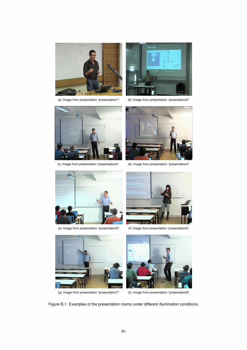
(a) Image from presentation “presentation1”. (b) Image from presentation “presentation2”.
(c) Image from presentation “presentation3”. (d) Image from presentation “presentation4”.
(e) Image from presentation “presentation5”. (f) Image from presentation “presentation6”.
(g) Image from presentation “presentation7”. (h) Image from presentation “presentation8”.
Figure B.1: Examples of the presentation rooms under different illumination conditions.
91
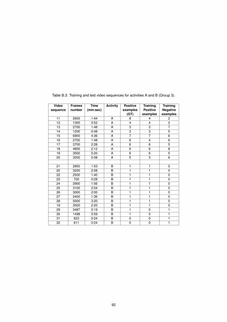
Table B.3: Training and test video sequences for activities A and B (Group 3).
Video Frames Time Activity Positive Training Trainingsequence number (min:sec) examples Positive Negative
(GT) examples examples11 2600 1:44 A 8 4 212 1300 0:52 A 4 4 213 2700 1:48 A 3 3 714 1200 0:48 A 3 3 515 6900 4:36 A 7 7 616 2700 1:48 A 6 4 617 3700 2:28 A 6 6 518 4800 2:12 A 6 6 819 3500 2:20 A 6 6 520 3200 2:08 A 5 3 6
21 2850 1:53 B 1 1 020 3200 2:08 B 1 1 022 2500 1:40 B 1 1 023 700 0:28 B 1 1 024 2900 1:56 B 1 1 025 3100 2:04 B 1 1 026 3000 2:00 B 1 1 027 2400 1:36 B 1 1 028 5000 3:20 B 1 1 019 3500 2:20 B 1 1 029 3487 2:19 B 1 0 130 1498 0:59 B 1 0 131 623 0:24 B 0 0 132 611 0:24 B 0 0 1
92
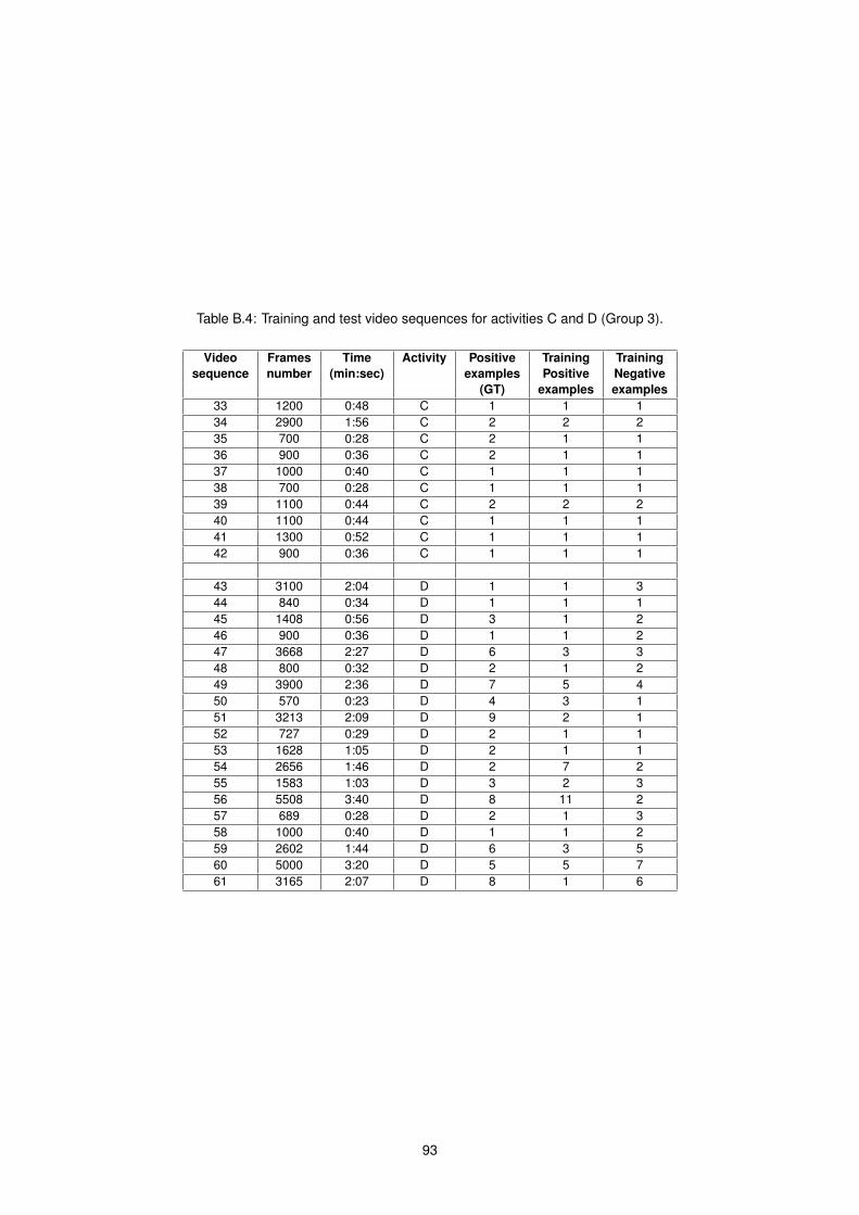
Table B.4: Training and test video sequences for activities C and D (Group 3).
Video Frames Time Activity Positive Training Trainingsequence number (min:sec) examples Positive Negative
(GT) examples examples33 1200 0:48 C 1 1 134 2900 1:56 C 2 2 235 700 0:28 C 2 1 136 900 0:36 C 2 1 137 1000 0:40 C 1 1 138 700 0:28 C 1 1 139 1100 0:44 C 2 2 240 1100 0:44 C 1 1 141 1300 0:52 C 1 1 142 900 0:36 C 1 1 1
43 3100 2:04 D 1 1 344 840 0:34 D 1 1 145 1408 0:56 D 3 1 246 900 0:36 D 1 1 247 3668 2:27 D 6 3 348 800 0:32 D 2 1 249 3900 2:36 D 7 5 450 570 0:23 D 4 3 151 3213 2:09 D 9 2 152 727 0:29 D 2 1 153 1628 1:05 D 2 1 154 2656 1:46 D 2 7 255 1583 1:03 D 3 2 356 5508 3:40 D 8 11 257 689 0:28 D 2 1 358 1000 0:40 D 1 1 259 2602 1:44 D 6 3 560 5000 3:20 D 5 5 761 3165 2:07 D 8 1 6
93
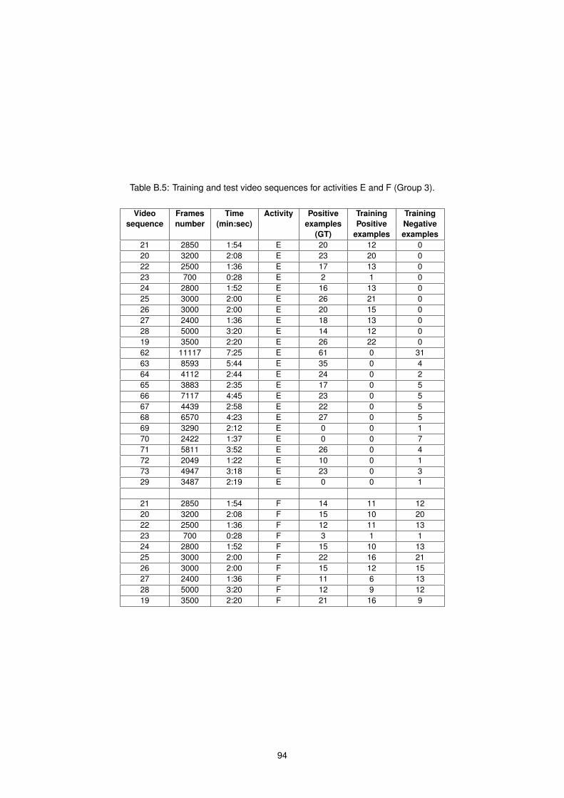
Table B.5: Training and test video sequences for activities E and F (Group 3).
Video Frames Time Activity Positive Training Trainingsequence number (min:sec) examples Positive Negative
(GT) examples examples21 2850 1:54 E 20 12 020 3200 2:08 E 23 20 022 2500 1:36 E 17 13 023 700 0:28 E 2 1 024 2800 1:52 E 16 13 025 3000 2:00 E 26 21 026 3000 2:00 E 20 15 027 2400 1:36 E 18 13 028 5000 3:20 E 14 12 019 3500 2:20 E 26 22 062 11117 7:25 E 61 0 3163 8593 5:44 E 35 0 464 4112 2:44 E 24 0 265 3883 2:35 E 17 0 566 7117 4:45 E 23 0 567 4439 2:58 E 22 0 568 6570 4:23 E 27 0 569 3290 2:12 E 0 0 170 2422 1:37 E 0 0 771 5811 3:52 E 26 0 472 2049 1:22 E 10 0 173 4947 3:18 E 23 0 329 3487 2:19 E 0 0 1
21 2850 1:54 F 14 11 1220 3200 2:08 F 15 10 2022 2500 1:36 F 12 11 1323 700 0:28 F 3 1 124 2800 1:52 F 15 10 1325 3000 2:00 F 22 16 2126 3000 2:00 F 15 12 1527 2400 1:36 F 11 6 1328 5000 3:20 F 12 9 1219 3500 2:20 F 21 16 9
94

Appendix C
Tracker Experimental Results
Table C.1: Tracker’s performance for speaker’s face and resolution 90x72
Sequence ex ey R M(0, 0) M(1, 0)
name M(0, 1) M(1, 1)1 -0.2 3.26 12.72 0.11 1 0
0.11 7.79 0 12 1.17 0.93 18.71 15.88 1 0
15.88 26.84 0.08 0.923 2 3.04 8.92 1.46 1 0
1.46 4.12 0.52 0.484 0.35 11.65 51.33 -9.43 1 0
-9.43 87.43 0.6 0.45 0.88 1.88 5.59 -0.13 1 0
-0.13 6.23 0 1
Table C.2: Tracker’s performance for speaker’s torso and resolution 90x72
Sequence Right boundary Left boundary M(0, 0) M(1, 0)
name ex σex ex σex M(0, 1) M(1, 1)1 5.72 5.18 -8.66 6.74 1 0
0 12 2.91 4.34 -7.98 5.79 1 0
0.08 0.923 -4.17 4.53 -6.21 3.54 1 0
0.52 0.484 -4.7 9.95 -3.2 7.64 1 0
0.6 0.45 1.4 6.34 -3.14 4.81 1 0
0 1
Table C.3: Tracker’s performance for speaker’s left hand and resolution 90x72
Sequence ex ey R M(0, 0) M(1, 0)
name M(0, 1) M(1, 1)1 3.06 2.83 12.97 3.92 1 0
3.92 6.54 0.2 0.82 5.77 -6.45 44.63 7.45 1 0
7.45 86.83 0.35 0.653 2.56 -7.44 27.62 22.68 0.63 0.38
22.68 40.87 0.62 0.384 4.5 -18.12 38.5 -68.06 1 0
-68.06 519.36 0.84 0.165 -0.58 -0.11 2.45 -0.38 1 0
-0.38 6.94 0.41 0.59
95
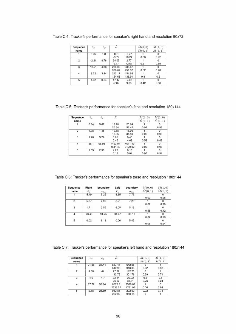
Table C.4: Tracker’s performance for speaker’s right hand and resolution 90x72
Sequence ex ey R M(0, 0) M(1, 0)
name M(0, 1) M(1, 1)1 -1.37 1.8 10.1 -3.77 1 0
-3.77 20.24 0.08 0.922 -2.21 8.76 94.05 2.77 1 0
2.77 72.67 0.31 0.693 12.21 4.38 288.08 386.67 1 0
386.67 751.32 0.52 0.484 9.22 3.44 242.17 154.68 1 0
154.68 136.91 0.8 0.25 1.62 0.54 17.47 -7.02 1 0
-7.02 9.63 0.42 0.58
Table C.5: Tracker’s performance for speaker’s face and resolution 180x144
Sequence ex ey R M(0, 0) M(1, 0)
name M(0, 1) M(1, 1)1 0.84 5.67 18.18 20.64 1 0
20.64 58.42 0.02 0.982 1.78 1.45 19.68 18.96 1 0
18.96 31.59 0.02 0.983 1.76 3.29 6.85 0.45 1 0
0.45 4.68 0.58 0.424 85.1 68.98 7463.97 4611.49 1 0
4611.49 3120.02 0.02 0.985 1.55 2.98 4.25 0.16 1 0
0.16 5.04 0.06 0.94
Table C.6: Tracker’s performance for speaker’s torso and resolution 180x144
Sequence Right boundary Left boundary M(0, 0) M(1, 0)
name ex σex ex σex M(0, 1) M(1, 1)1 5.49 5.25 -3.65 7.73 1 0
0.02 0.982 5.37 2.92 -8.71 7.26 1 0
0.02 0.983 1.71 3.56 -8.05 5.18 1 0
0.58 0.424 73.49 91.75 84.47 85.19 1 0
0.02 0.985 0.02 6.18 -0.06 5.49 1 0
0.06 0.94
Table C.7: Tracker’s performance for speaker’s left hand and resolution 180x144
Sequence ex ey R M(0, 0) M(1, 0)
name M(0, 1) M(1, 1)1 21.58 38.44 857.45 642.98 0 1
642.98 918.06 0.02 0.982 4.88 -8 97.22 112.76 0 1
112.76 301.76 0.29 0.713 4.6 -4.7 32.44 26.02 0.5 0.5
26.02 38.81 0.76 0.244 87.72 59.94 6076.8 2538.02 1 0
2538.02 1761.08 0.06 0.945 2.88 25.69 952.86 222.02 0.22 0.78
222.02 958.15 0 1
96

Table C.8: Tracker’s performance for speaker’s right hand and resolution 180x144
Sequence ex ey R M(0, 0) M(1, 0)
name M(0, 1) M(1, 1)1 -3.82 28.65 1541.54 -65.34 1 0
-65.34 1029.94 0.02 0.982 -1.86 6.4 82.07 -14.33 0 1
-14.33 112.8 0.1 0.93 7.6 -1.9 33.44 16.19 1 0
16.19 86.09 0.6 0.44 34.05 80.83 3495.62 806.25 0 1
806.25 1391.95 0.05 0.955 -17.36 34.83 770.23 -468.35 0 1
-468.35 1102.19 0.07 0.93
Table C.9: Tracker’s performance for speaker’s face and resolution 360x288
Sequence ex ey R M(0, 0) M(1, 0)
name M(0, 1) M(1, 1)1 1.36 6.7 17.35 19.89 1 0
19.89 66.45 0 12 1.41 1.16 11.79 2.5 1 0
2.5 3.77 0.02 0.983 1.44 2.82 52.33 -2.62 1 0
-2.62 7.95 0 14 0.07 8.5 8.21 -7.75 1 0
-7.75 58.54 0.72 0.285 1.76 3.5 4.7 -0.86 1 0
-0.86 4.81 0 1
Table C.10: Tracker’s performance for speaker’s torso and resolution 360x288
Sequence Right boundary Left boundary M(0, 0) M(1, 0)
name ex σex ex σex M(0, 1) M(1, 1)1 6.6 5.18 -3.48 8.57 1 0
0 12 5.61 3.14 -7 3.72 1 0
0.02 0.983 2.9 10.5 -7.12 8.05 1 0
0 14 0.71 6.8 -8.07 7.82 1 0
0.72 0.285 2.56 6.2 0.16 5.83 1 0
0 1
Table C.11: Tracker’s performance for speaker’s left hand and resolution 360x288
Sequence ex ey R M(0, 0) M(1, 0)
name M(0, 1) M(1, 1)1 49.98 55.61 586.34 213.08 0 1
213.08 302.46 0 12 -1.35 -5.3 391.63 178.84 0 1
178.84 230.05 0.23 0.773 4.47 0.21 251.37 226.61 0 1
226.61 583.4 0.19 0.814 1.77 -23.38 165.41 369.99 1 0
369.99 1317.93 0.74 0.265 8.8 11.43 719.16 416.42 0.11 0.89
416.42 701.18 0.06 0.94
97
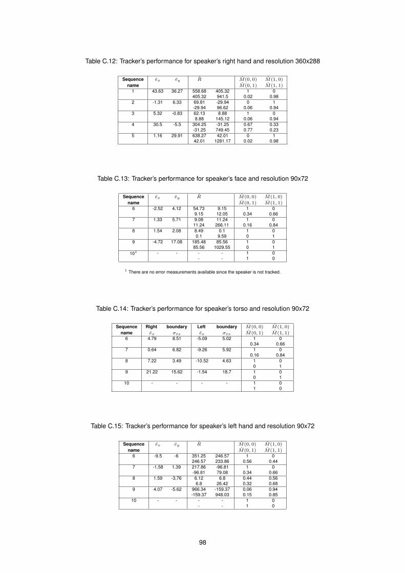
Table C.12: Tracker’s performance for speaker’s right hand and resolution 360x288
Sequence ex ey R M(0, 0) M(1, 0)
name M(0, 1) M(1, 1)1 43.63 36.27 558.68 405.32 1 0
405.32 941.5 0.02 0.982 -1.31 6.33 69.81 -29.94 0 1
-29.94 96.62 0.06 0.943 5.32 -0.83 62.13 8.88 1 0
8.88 145.12 0.06 0.944 30.5 -5.5 304.25 -31.25 0.67 0.33
-31.25 749.45 0.77 0.235 1.16 29.91 638.27 42.01 0 1
42.01 1281.17 0.02 0.98
Table C.13: Tracker’s performance for speaker’s face and resolution 90x72
Sequence ex ey R M(0, 0) M(1, 0)
name M(0, 1) M(1, 1)6 -2.52 4.12 54.73 9.15 1 0
9.15 12.05 0.34 0.667 1.33 5.71 9.08 11.24 1 0
11.24 266.11 0.16 0.848 1.54 2.08 8.49 0.1 1 0
0.1 9.59 0 19 -4.72 17.08 185.48 85.56 1 0
85.56 1029.55 0 1101 - - - - 1 0
- - 1 0
1 There are no error measurements available since the speaker is not tracked.
Table C.14: Tracker’s performance for speaker’s torso and resolution 90x72
Sequence Right boundary Left boundary M(0, 0) M(1, 0)
name ex σex ex σex M(0, 1) M(1, 1)6 4.79 8.51 -5.09 5.02 1 0
0.34 0.667 0.64 6.82 -9.26 5.92 1 0
0.16 0.848 7.22 3.49 -10.52 4.63 1 0
0 19 21.22 15.62 -1.54 18.7 1 0
0 110 - - - - 1 0
1 0
Table C.15: Tracker’s performance for speaker’s left hand and resolution 90x72
Sequence ex ey R M(0, 0) M(1, 0)
name M(0, 1) M(1, 1)6 -9.5 -6 351.25 246.57 1 0
246.57 233.86 0.56 0.447 -1.58 1.39 217.86 -96.81 1 0
-96.81 79.08 0.34 0.668 1.59 -3.76 6.12 6.8 0.44 0.56
6.8 26.42 0.32 0.689 4.07 -5.62 966.34 -159.37 0.06 0.94
-159.37 948.03 0.15 0.8510 - - - - 1 0
- - 1 0
98

Table C.16: Tracker’s performance for speaker’s right hand and resolution 90x72
Sequence ex ey R M(0, 0) M(1, 0)
name M(0, 1) M(1, 1)6 3.31 0.77 113.29 -23.31 1 0
-23.31 11.1 0.73 0.277 -3.26 14.39 204.98 -518.03 0.89 0.11
-518.03 1530.5 0.44 0.568 0.78 0.65 4.37 -0.93 1 0
-0.93 3.28 0.18 0.829 0.33 -19.53 617.43 -253.22 1 0
-253.22 787.74 0.14 0.8610 - - - - 1 0
- - 1 0
Table C.17: Tracker’s performance for speaker’s face and resolution 180x144
Sequence ex ey R M(0, 0) M(1, 0)
name M(0, 1) M(1, 1)6 -2.51 2.95 39.43 8.2 1 0
8.2 7.38 0.22 0.787 -13.88 23.47 1314.8 -1516.89 1 0
-1516.89 2034.71 0.14 0.868 1.26 2.16 28.79 0.26 1 0
0.26 8.61 0 19 -4.52 3.36 41.65 -4.35 1 0
-4.35 21.83 0 110 - - - - 1 0
- - 1 0
Table C.18: Tracker’s performance for speaker’s torso and resolution 180x144
Sequence Right boundary Left boundary M(0, 0) M(1, 0)
name ex σex ex σex M(0, 1) M(1, 1)6 5.54 7.67 -3.77 5.8 1 0
0.22 0.787 -14.79 41.28 -21.79 30.04 1 0
0.14 0.868 9.38 4.82 -15.04 6.4 1 0
0 19 23.06 8.29 -3.78 9.5 1 0
0 110 - - - - 1 0
1 0
99

Table C.19: Tracker’s performance for speaker’s left hand and resolution 180x144
Sequence ex ey R M(0, 0) M(1, 0)
name M(0, 1) M(1, 1)6 3.35 2.55 547.93 270.46 0.89 0.11
270.46 150.35 0.38 0.637 -30.32 15.12 3374.16 -1603.61 0.67 0.33
-1603.61 1241.46 0.28 0.728 -20.06 -47.29 115.82 22.04 0.2 0.8
22.04 316.21 0.32 0.689 26.97 -23.23 1178.74 -242.43 0 1
-242.43 914.56 0.09 0.9110 - - - - 1 0
- - 1 0
Table C.20: Tracker’s performance for speaker’s right hand and resolution 180x144
Sequence ex ey R M(0, 0) M(1, 0)
name M(0, 1) M(1, 1)6 4.88 -2.69 515.87 -107.7 1 0
-107.7 410.21 0.46 0.547 -30.06 32.97 3438.6 -2521.61 0.11 0.89
-2521.61 2538.82 0.2 0.88 1.69 -0.8 54.04 -58.89 0 1
-58.89 222.87 0.08 0.929 12.84 -34.31 1045.51 -49.98 1 0
-49.98 2132.84 0.1 0.910 - - - - 1 0
- - 1 0
Table C.21: Tracker’s performance for speaker’s face and resolution 360x288
Sequence ex ey R M(0, 0) M(1, 0)
name M(0, 1) M(1, 1)6 -2 3.74 48.11 10.5 1 0
10.5 7.35 0.24 0.767 2.03 2.79 5 -1.24 1 0
-1.24 9.56 0.34 0.668 2.04 4.26 6.92 -0.65 1 0
-0.65 14.19 0 19 -4.7 2.12 61.77 8.22 1 0
8.22 49.47 0 110 - - - - 1 0
- - 1 0
Table C.22: Tracker’s performance for speaker’s torso and resolution 360x288
Sequence Right boundary Left boundary M(0, 0) M(1, 0)
name ex σex ex σex M(0, 1) M(1, 1)6 7.18 8.41 -4.18 5.62 1 0
0.24 0.767 4.48 4.43 -10.48 4.3 1 0
0.34 0.668 9.78 4.22 -7.86 3.91 1 0
0 19 26.16 10.13 -0.92 13.35 1 0
0 110 - - - - 1 0
1 0
100

Table C.23: Tracker’s performance for speaker’s left hand and resolution 360x288
Sequence ex ey R M(0, 0) M(1, 0)
name M(0, 1) M(1, 1)6 -10.45 -11.91 703.79 479.77 0.72 0.28
479.77 889.99 0.31 0.697 2.52 -0.52 20.06 12.49 1 0
12.49 19.6 0.34 0.668 -9.48 -14.33 270.06 290.22 0.04 0.96
290.22 455.17 0.16 0.849 23.09 -52.71 710.67 48.8 0 1
48.8 1357.44 0 110 - - - - 1 0
- - 1 0
Table C.24: Tracker’s performance for speaker’s right hand and resolution 360x288
Sequence ex ey R M(0, 0) M(1, 0)
name M(0, 1) M(1, 1)6 1.3 -5.67 248.54 -86.67 1 0
-86.67 514.62 0.38 0.637 1.71 13.33 68.59 20.95 0.11 0.89
20.95 410.32 0.49 0.518 2.49 4.04 203.91 -132.87 1 0
-132.87 284.64 0.04 0.969 44.86 -69.9 989.06 -344.6 1 0
-344.6 4079.32 0.02 0.9810 - - - - 1 0
- - 1 0
101

Appendix D
Speed Measurements
Table D.1: Tracker’s speed over three image resolutions for Group 1 and 2 (Tables B.1-B.2).
Sequence Resolution/fpsname 90x72 180x144 360x2881.avi 62.87 47.62 19.382.avi 63.14 55.31 22.773.avi 63.25 40.27 22.714.avi 62.74 60.63 24.385.avi 63.09 49.36 21.93
Average Group 1 63.02 50.64 22.236.avi 63.53 40.18 18.247.avi 63.05 53.19 21.268.avi 63.12 55.42 27.979.avi 62.46 34.97 14.1310.avi 63.58 34.15 17.80
Average Group 2 63.15 43.58 19.88
Table D.2: System’s speed over three image resolutions (tracking, video recording and activity recognition) forGroup 1 and 2 (Tables B.1-B.2).
Sequence Resolution/fpsname 90x72 180x144 360x2881.avi 39.07 32.53 17.902.avi 40.54 34.60 19.433.avi 49.36 34.38 21.504.avi 50.99 34.48 19.225.avi 36.92 31.70 19.77
Average Group 1 43.37 33.54 19.576.avi 41.58 33.13 16.567.avi 38.68 34.08 19.188.avi 39.78 34.52 20.549.avi 36.95 26.57 13.0610.avi 59.61 34.09 17.25
Average Group 2 43.32 32.48 17.32
102