Tracking Moving Objects From a Moving VehicleUsing a Laser Scanner

Robert MacLachlan

CMU-RI-TR-05-07

The Robotics Institute Carnegie Mellon University

5000 Forbes Avenue Pittsburgh, PA 15213

June 23, 2005

©2005, 2006 Carnegie Mellon University

Table of ContentsChapter 1: Introduction.....................................................................................................................1

1.1: Sensor Characteristics.......................................................................................................... 21.2: Tracking with Laser Scanners vs. Other Sensors.................................................................31.3: The Tracking Problem..........................................................................................................4

1.3.1: Shape Change............................................................................................................... 41.3.2: Occlusion......................................................................................................................51.3.3: 2D Scan of a 3D World................................................................................................ 61.3.4: Vegetation.................................................................................................................... 61.3.5: Weak Returns............................................................................................................... 71.3.6: Drippy Points................................................................................................................71.3.7: Clutter...........................................................................................................................8

Chapter 2: Tracker Structure and Algorithms.................................................................................. 92.1: Simple Segmentation............................................................................................................9

2.1.1: Partial Occlusion Detection..........................................................................................92.2: Geometric Object Modeling............................................................................................... 10

2.2.1: Corner Fitting............................................................................................................. 112.2.2: Shape classification.................................................................................................... 12Note that when model-based segmentation is enabled we don't use the COMPLEX shape classification, and always force the best line/corner match to be used. This works fine, and reduces the number of special cases that need to be handled. Though a line may be a poor approximation of an arbitrary shape, it is still no worse than a bounding box, and probably better. In this case, the min/max bound features become a historical vestige.................... 13

2.3: Data Association.................................................................................................................132.3.1: Overlap Based Association........................................................................................ 142.3.2: Track Splitting and Merging...................................................................................... 142.3.3: Maximum Closeness.................................................................................................. 142.3.4: Feature Correspondence.............................................................................................152.3.5: Track Creation and Death.......................................................................................... 15

2.4: Model-Based Segmentation................................................................................................162.4.1: Segmentation Using Model Distance.........................................................................162.4.2: Top-Down Data Association...................................................................................... 162.4.3: Track Splitting (and not merging)..............................................................................172.4.4: Implementation issues................................................................................................ 17

2.5: Track State and Dynamic Model........................................................................................182.5.1: Rotational Estimation.................................................................................................182.5.2: Tracking Features....................................................................................................... 192.5.3: Track Center............................................................................................................... 192.5.4: Feature noise model....................................................................................................20

Vague Line Ends............................................................................................................. 21Noise Adaptation.............................................................................................................21

2.5.5: Information Increment Test........................................................................................222.5.6: Improving the Kalman Filter for Outliers.................................................................. 222.5.7: Track Startup.............................................................................................................. 23

2.6: Track Validation.................................................................................................................232.7: Total Occlusion Detection..................................................................................................25

Chapter 3: Evaluation..................................................................................................................... 273.1: Tracker prediction error vs. time horizon...........................................................................283.2: Sensitivity of Track validation Parameters........................................................................ 28

Chapter 4: Unfinished Work...........................................................................................................304.1: Time Skew..........................................................................................................................304.2: Multiple Scanners...............................................................................................................304.3: Track classification based on shape/texture.......................................................................314.4: Time Consistency............................................................................................................... 32

4.4.1: Shape constancy......................................................................................................... 324.5: General Classification........................................................................................................ 344.6: Improved Estimation.......................................................................................................... 35

Illustration IndexIllustration 1: Angular Resolution Effects 2Illustration 2: Shape Change Example 5Illustration 3: Occlusion 6Illustration 4: Vegetation 7Illustration 5: Weak Returns 8Illustration 6: Robust Corner Matching 11Illustration 7: Features 13Illustration 8: Point Spacing Effect of Angular Resolution 20Illustration 9: History Matching 24Illustration 10: Tracker Output 27Illustration 11: Estimated Prediction Error 28Illustration 12: Moving Test Performance 29

1

Chapter 1: IntroductionThis report describes software developed for the tracking of vehicles and pedestrians using scanning laser rangefinders mounted on a moving vehicle. Although the system combines various algorithms and empirical decision rules to achieve acceptable performance, the basic mechanism is tracking of line features, so we call this approach linear feature tracking.

Much of the work in the report is also summarized in [MacLachlan06], which should probably be read first. See also http://www.cs.cmu.edu/~ram/tracking/ for papers and movies. The source code is (in by biased opinion) of high quality, and may also be available, but would not work outside of the NavLab software architecture without some modification.

This illustration is a portion of an input frame from the laser rangefinder:

This illustration is a visualization of the tracker output, and gives some idea of what the tracker does. The numbers are track identifiers. Track 38 (brown) is a car moving at 5.7 meters/sec and turning at 21 degrees/sec. The light blue arc drawn from track 38 is the projected path over the next two seconds. The other tracks are non-moving clutter objects such as trash cans and light poles. The actual scanner data points are single pixel dots. The straight lines have been fitted to these points. An X is displayed at the end of the line if we are confident that the line end represents a corner.

There are three major parts to this presentation:

2

• Introduction of the sensor characteristics, comparison with other tracking problems, and discussion of some specific problematic situations.

• Presentation of the structure and algorithms used by the tracker.• Discussion of the performance and limitations of the current system.

1.1: Sensor CharacteristicsA laser rangefinder (or LIDAR) is an active optical position measurement sensor. Using the popular time-of-flight measurement principle, a laser pulse is sent out by the sensor, reflects off of an object in the environment, then the elapsed time before arrival of the return pulse is converted into distance. In a scanning laser rangefinder, mechanical motion of a scanning mirror directs sequential measurement pulses in different directions, permitting the building of an approximation of a 2D model of the environment (3D with two scan axes.) We will use the term scanner as a shorter form of scanning laser rangefinder.

The scanning mirror moves continuously, but measurements are made at discrete angle increments. Though this is not actually how the scanner operates, the effects of angular quantization are easier to understand if you visualize the scanner as sending out a fixed pattern of light beams which sweep across the environment as the scanner moves (sort of like cat whiskers, see illustration 1.)

• When viewed in the natural polar coordinates, the rotational (azimuth) and radial (range) measurement error are due to completely different processes, and have different range dependence:

Illustration 1: Angular Resolution Effects

3

• The azimuth error is primarily due to the angular quantization, though this is related to the underlying physical consideration of laser spot size. For a given beam incidence angle on the target, the Cartesian position uncertainty is proportional to the range.

• The range measurement error comes from the per-pulse range measurement process, and in a time-of-flight system is largely due to the timer resolution. This results in a range accuracy that is independent of distance.

Linear feature tracking was developed for a collision warning system for transit buses. This system uses the SICK LMS 200, which is a scanning laser rangefinder with a single scan axis. The scanner is oriented to scan in a horizontal plane, and all processing is done using 2D geometry in this scan plane. Performance specifications are 1cm range resolution, 50 meter range, 1 degree basic azimuth resolution and 75 scans/second. The output of the scanner is simply a vector of 181 range values. If the measurement process fails due to no detectable return, this is flagged by a distinct large range value.

Note that with these range and angle resolutions, the position uncertainty is dominated by azimuth quantization throughout the entire useful operating range. At a practical extreme range of 20 meters, a one degree arc is 34cm, whereas the range resolution is still 1cm.

The LMS 200 also has a 0.5 degree 38 scan/sec operating mode which interlaces two 1 degree scans. The higher angular resolution is very desirable, but because of the time skew between adjacent points, this mode is not very usable when speeds are above 3 meters/sec. In future work we plan to remove these interlace artifacts by compensating for the time skew.

1.2: Tracking with Laser Scanners vs. Other Sensors

The problem of tracking moving objects using a scanning laser rangefinder is in some ways intermediate in characteristics between long range radar tracking (e.g. of aircraft) and computer vision tracking.

What advantages for object tracking does a laser scanner have over computer vision? Two difficult problems in vision based tracking are• Position: determination of the position of objects using vision can only be done using

unreliable techniques such as stereo vision or assuming a particular object size. Position determination is trivial using ranging sensors like radar and laser scanners, as long as there is adequate angular resolution,

• Segmentation: when two objects appear superimposed by our perspective, how can we tell where one ends and the next begins? Range measurement makes segmentation much easier because foreground objects are clearly separated from the background.

An important problem that laser scanners have in common with computer vision is point correspondence given two measurements of the same object, which specific measurements correspond to the same point on the object.

In long range radar, the point correspondence problem typically doesn't exist -- the object size is at or below the angular resolution, so the object resembles a single point. In contrast, when a

4

laser scanner is used in an urban driving situation, we need to be able to track objects whose size is 10 to 100 times our angular resolution. Not only do the tracked vehicles not resemble points, after taking into consideration the effect of azimuth resolution, they often effectively extend all the way to the horizon in one direction.

When the size of objects can't be neglected, this creates ambiguity in determining the position of the object (what point to use). Since a tracker estimates dynamics such as the velocity by observing the change in position over time, this position uncertainty can create serious errors in the track dynamics.

As in computer vision, the extended nature of objects does also have some benefits. Because we have multiple points on each object, we can make use of this additional information to classify objects (bush, car, etc.)

1.3: The Tracking ProblemGiven this sensor, we would like to identify moving objects, determine the position and velocity, and also estimate higher order dynamics such as the acceleration and turn rate. The tracker must also be computationally efficient enough so that it can process 75 scans a second in an embedded system with other competing processes.

A track is an object identity annotated with estimates of dynamics derived by observing the time-change. The function of the tracker is to generate these tracks from a time-series of measurements. The purpose of maintaining the object identity is twofold: 1. We need to establish object correspondences from one measurement to the next so that we

can estimate dynamics.2. The object identity is in itself useful as it allows us to detect when objects appear and

disappear.

In general, tracking can be described as a three-step process which is repeated each time a new measurement is made:1. Predict the new position of each existing track based on the last estimate of position and

motion.2. Associate measurement data with existing tracks. If there is no good match, consider making

a new track.3. Estimate new position and motion based on the difference between the predicted position and

the measured one.

1.3.1: Shape Change

It is a crucial aspect of the tracking problem considered here that the laser rangefinder is itself in motion. If the scanner is not moving, the problem of detecting moving objects is trivial: just look for any change in the sensor reading. Once the scanner is moving, we expect fixed objects to appear to move in the coordinates of the scanner, and can correct for this with a coordinate transformation.

5

It is assumed that the motion of the rangefinder is directly measured, in our case by a combination of odometry and an inertial turn rate sensor. Since tracking is done over relatively short ranges and short periods of time, the required accuracy of the rangefinder motion estimate is not great, and relatively inexpensive sensors can be used.

The more intractable difficulty related to scanning from a moving vehicle is that, even after object positions are corrected by a coordinate transform, the appearance still changes when we move due to the changing scanner perspective. The scanner only sees the part of the object surface currently facing the scanner. As the scanner moves around a fixed object, we see different contours of the object surface.

The shape change doesn't cause any serious difficulty for determining that scan data corresponds to the same object from one scan to the next because the change is small. What is difficult is determining that these small changes are due to changes in perspective, and not actual motion of the tracked object.

To get a sense of the shape change problem, consider a naive algorithm which considers the object position to be the mean position of the object's measured points (see illustration 2.) Suppose that we are driving past a parked car. At time 1, we see only the end of the car. At time 2, we see both the side and end. By time 3, we only see the side. During this process, the center of mass of the point distribution shifts to the left, giving the parked car a velocity moving into our path, causing a false collision prediction. The point distribution also moves in our direction of motion creating false velocity in that direction.

1.3.2: Occlusion

Another problematic situation occurs when a small object moves in front of a larger background object. In this case, what is in effect the shadow of the foreground object creates a false moving

Illustration 2: Shape Change Example

6

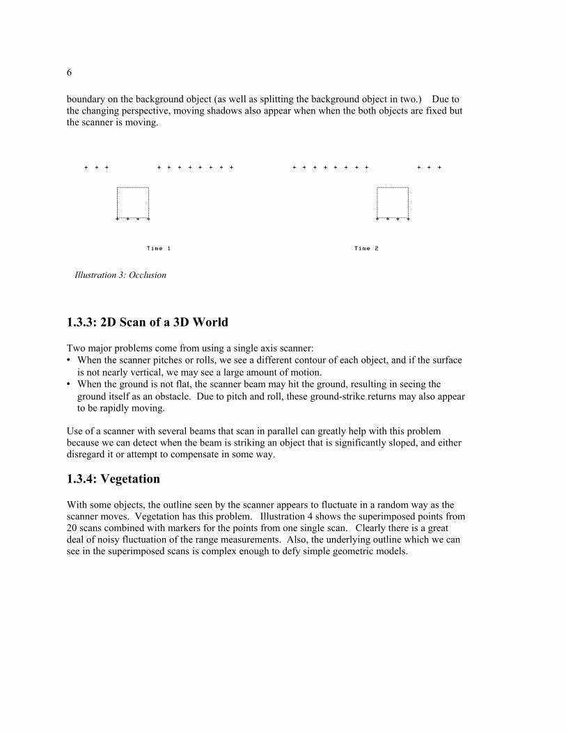
boundary on the background object (as well as splitting the background object in two.) Due to the changing perspective, moving shadows also appear when when the both objects are fixed but the scanner is moving.

1.3.3: 2D Scan of a 3D World

Two major problems come from using a single axis scanner:• When the scanner pitches or rolls, we see a different contour of each object, and if the surface

is not nearly vertical, we may see a large amount of motion.• When the ground is not flat, the scanner beam may hit the ground, resulting in seeing the

ground itself as an obstacle. Due to pitch and roll, these ground-strike returns may also appear to be rapidly moving.

Use of a scanner with several beams that scan in parallel can greatly help with this problem because we can detect when the beam is striking an object that is significantly sloped, and either disregard it or attempt to compensate in some way.

1.3.4: Vegetation

With some objects, the outline seen by the scanner appears to fluctuate in a random way as the scanner moves. Vegetation has this problem. Illustration 4 shows the superimposed points from 20 scans combined with markers for the points from one single scan. Clearly there is a great deal of noisy fluctuation of the range measurements. Also, the underlying outline which we can see in the superimposed scans is complex enough to defy simple geometric models.

Illustration 3: Occlusion

7

1.3.5: Weak Returns

Some objects have very poor reflectivity at the infrared frequency where the SICK scanner operates. Illustration 5 shows an example of a car that is almost invisible to the scanner. During the 10 seconds that we drive by, we are able to build up a reasonably complete idea of the car (small dots), apparently largely from specular glints. However, on any given scan, very little of the car is visible. In this particular single scan, we are mainly seeing inside the wheel wells (oblong areas area inside outline box.) Evidently the dirt inside the wheel well is a better reflector than the paint.

1.3.6: Drippy Points

The Sick exhibits a particular measurement error where on a range step it gives readings intermediate between the two ranges: the points appear to “drip” off the end of the nearer object. This perturbs the true end positions and may also cause disjoint objects to be spuriously segmented together.

Illustration 4: Vegetation

8

1.3.7: Clutter

Another cause of unclear object outlines is clutter: when objects are close together. In this case, it isn't clear whether to segment the data as one or two objects. If the segmentation flips between one and two objects, this causes apparent shape change. Clutter can also cause spurious disappearance of tracks, for example when a pedestrian moves close to a wall, and appears to merge with the wall.

Illustration 5: Weak Returns

9

Chapter 2: Tracker Structure and AlgorithmsThese are the major parts of the tracker:• Segmentation: group scanner points according to which object they are part of.• Model fitting: summarize points with a geometric model (rectangle.)• Data association: find the existing track corresponding to the new measurements.• Dynamic model and Kalman filter: determine velocity, acceleration and turn rate from the

raw position measurements.• Track validation: assess the validity of the dynamic estimate and see if the track appears to be

moving.

There are 85 parameters used by the tracker. For concreteness and conciseness, we will refer to the specific numeric values that have been empirically tuned for our particular scanner and application, rather than to parameter names. Generally the parameter values are not all that sensitive, but for best performance with a different scanner or application, different values would be used.

Also, since the source code is available and well commented, we will avoid in-depth discussion of implementation details better read from the source. In particular, although efficiency is one of the important characteristics of the tracker, we won't do much in-depth discussion of performance-related issues.

2.1: Simple SegmentationSimple segmentation takes the list of range and azimuth points returned by the scanner and partitions it into sublists of contiguous points. In simple segmentation, two neighboring points are considered part of the same object if the separation is less than 0.8 meters. After simple segmentation, the points are converted into a non-moving Cartesian coordinate system by transforming out the effects of the known motion of the scanner.

Simple segmentation is called simple to contrast with Model Based Segmentation (section 2.4), which refines the segmentation when objects are not well separated. In contrast to the top-down process of model-based segmentation, simple segmentation is purely bottom up. The simple segmentation is used to maintain the validity of the model used in model-based segmentation .

Also, if the model_based_segmentation parameter is false, simple segmentation can be used exclusively.

2.1.1: Partial Occlusion Detection

During simple segmentation we also detect when background objects are partially occluded by foreground objects. Each point is classified as occluded or normal. A point is occluded if an adjacent point in the scan is in a different segment and in front of this point, or if it is the first or last point in the scan. This flag has several uses:

10

• When an occluded point appears at the boundary of an object, we consider this to be a false boundary.

• We only count non-occluded points when determining if there enough points to create a new track or if the point density is high enough for a segment to be compact.

• If an occluded point defines the position of a feature, then that feature is vague.

In segmentation, missing range returns are treated as points at maximum distance, and are not assigned to any segment. If there is a large enough dropout in the middle of an object, it will split the object into two segments.

If any point in a segment is occluded, then segment is considered partially occluded. Tracks that are not associated on the current tracker iteration, and which were last associated with a partially occluded segment are considered for possible total occlusion. Detection of tracks are are totally occluded is a separate process described the Total Occlusion Detection section, 2.7.

2.2: Geometric Object ModelingThe use of a geometric model to summarize measured points is very important because it:• Locates features that tend to have stable locations even during motion-induced shape change, • Allows us to measure how well the data conforms to the model, helping in object

classification, and• Reduces the data to make processing more efficient.

Currently, only line or rectangle models are used. This is not as limiting as it might seem because vehicles are well-modeled as rectangles, and even for objects that do not have a good linear fit, like people or tree trunks, a line or rectangle is a fair summary of the space occupied by the object.

For each segment, we do a least-squares fit to a line and to a right-angle corner. Since the stability of feature locations is crucial for accurate velocity measurement, there are two refinements to the basic least-squares fit:• Points are weighted proportional to their separation along the line. Since some parts of the

object may be much closer than others, the point density along the object contour can vary a great deal. This weighting reduces problems with rounded corners that have high point density causing the line fit to rotate away from more distant points that actually contain more information about the overall rectangular shape approximation.

• The 20% of points with worst unweighted fit are discarded, then we refit. Although this reduces sensitivity to outliers from any source, the scanner has little intrinsic noise, so the effect is mainly on real object features that violate the rectangular model, notably rounded corners and wheel wells.

Because conceptually both the point spacing (distance along the line) and fit error (distance normal to the line) depend on the line, which is what we are trying to find the the first place, we use an iterative approximation. Each line fit requires three least-squares fits:1. An equal-weight least-squares fit of all the points in the segment. This is used to determine

the point spacing for weighting.2. Trial weighted fit, used to determine the outlier points. 3. Final weighted fit.

11

The position of each line end point is determined by taking the ending point in the input points and finding the closest point lying on the fitted line.

2.2.1: Corner Fitting

Corner fitting is done after fitting as a line. This is a somewhat degenerate case of a poly-line simplification algorithm. We split the point list in two at the knuckle point: the point farthest from the line fit. The geometrically longer side is then fit as a line. Since we constrain the corner to a right angle, the long side fit determines the direction of the short side. All we need to do is determine the location of the short side, which is done by taking the mean position along the long side of the short-side points. The location of the corner itself is the intersection of the two sides.

When doing the corner fit, we test for the corner being well-defined (approximately right angle) by doing an unconstrained linear fit on the short side, and testing the angle between the two sides. The angle must be at least 50 degrees away from parallel to be considered a good fit.

The corner must also be convex, meaning that the point of the corner aims toward the scanner (hence away from the interior of the opaque object.) We impose this restriction because in practice concave corners only appear on large fixed objects like walls, not on moving objects.

Illustration 6 is an example of corner fitting in the presence of corner rounding, outliers and variable point spacing. The fit matches the overall outline accurately fairly accurately.

Illustration 6: Robust Corner Matching

12

2.2.2: Shape classification

After fitting and line and corner, each segment is given a shape classification: corner Corner fit mean-squared error less than line fit and less than 10 cm.

line Line fit mean-squared error less than 10cm. complex Fall-back shape class for objects with poor linear fit having only a bounding box.

There are two boolean shape attributes which are semi-independent from the shape-class:

compact Diagonal of bounding box < 0.7 meters and point density > 5 points/meter. The compact criterion is chosen so that pedestrians will be compact (as will lamp-posts, fire hydrants, etc.) Because compact objects are small, we can estimate their velocity reasonably accurately without having a good linear fit.

disoriented Rotation angle not well defined. True if the line or long side of corner has less than 6 points, the RMS fit is worse than 4 cm, or the line and corner fit disagree by more than 7 degrees and the chosen classification's RMS error is less than 4 times better than the alternative. Segments that are complex or < 0.7 meters diagonal are always disoriented.

The disoriented attribute is used to determine whether to use the change in orientation to estimate turn rate. Also, if a segment is disoriented and not compact, then it has a poor linear fit, and we are more skeptical of the motion estimate.

Due to the restrictions of single-scanner perspective and 90 degree convex corners, there is a small fixed set of possible features that a segment can have (see illustration 7):

min, max The two diagonal corners of the bounding box (in world coordinates.) Defined for all shape classes.

first, last End points in a line segment, ends of the two sides in a corner segment.corner Corner point in a corner segment.center Rough estimate of object center derived from other features. Defined for all

shape classes.

13

Note that when model-based segmentation is enabled we don't use the COMPLEX shape classification, and always force the best line/corner match to be used. This works fine, and reduces the number of special cases that need to be handled. Though a line may be a poor approximation of an arbitrary shape, it is still no worse than a bounding box, and probably better. In this case, the min/max bound features become a historical vestige.

2.3: Data AssociationData association is the process of determining which current measurements correspond to existing tracks (or track features.) Model-based segmentation (section 2.4.2) can maintain a data association between tracks as long as the prior tracks are correct. However, this is not the case when new objects appear, old objects disappear, or existing objects split or merge.

Data association takes the results of simple segmentation and determines which tracks (if any) may be associated with the points underlying each simple segment. When there is no clear one-to-one correspondence between simple segments and tracks, then we defer to model-based segmentation.

In the context of the long-range tracking literature, our approach is basically nearest-neighbor. We pick one single segment in the measurement data which most closely resembles the prediction and use that for the new estimate. However, since each segment has many 2D points, the concept of “distance” is rather complex.

Our first approach to data association used the combined likelihood of the feature positions as a distance measure, then chose the most likely segment. However, we found this approach performed poorly, in that it both created bad tracks by associating separate objects and also

Illustration 7: Features

14

caused good tracks to break up if the object shape changed too much. To the human eyeball the errors seemed rather silly.

2.3.1: Overlap Based Association

We now use an approach based primarily on spatial overlap between the track and the measurement data. The concept of overlap-based association is simple: given rectangles representing the outlines of the track and the measurement, the two are associated if the outlines overlap.

The actual overlap algorithm is somewhat different, and handles non-rectangular objects much better. For two objects to overlap, we require that at least one actual measurement point fall inside the expanded track outline, and symmetrically, that when the track's last measured points are updated for predicted motion, that at least one of these predicted points falls inside the segment's outline. Since the points are on the edge of the object, we expand the object outline by 0.8 meters, then check if any points fall inside this expanded outline.

This algorithm works well even when a moving track passes though a concave part of a large fixed object (wall, etc.) In this case, none of the wall's points fall inside the track outline, even though the bounding box for the wall may entirely enclose the track.

2.3.2: Track Splitting and Merging

In addition to its robustness, another advantage of overlap-based association is that it leads to a straightforward way of detecting when tracks split or merge. In these cases, overlap does not establish a one-to-one correspondence between tracks and segments. If a track splits, then there will be two segments overlapping the track. If two tracks merge, then there will be two tracks overlapping one segment.

Actual splitting or merging can happen when pedestrians get into or out of vehicles. In practice, segmentation errors are the most common cause of splitting and merging. In the presence of clutter, an object may appear to split from or merge with another nearby object. Missing returns can also cause holes in the middle of objects, causing them to split in two.

Whatever the cause, it is important to detect when tracks merge because it is a common reason for track disappearance. See section 2.3.5, Track Creation and Death, where we discuss the “died without offspring” test.

When two tracks join, the ID of the merged track is that of the older track.

2.3.3: Maximum Closeness

In addition to split/merge situations, our fairly permissive overlap test can also generate complex overlap relationships when tracks are simply close together. Since in general the overlap test may create a many-to-many association between tracks and segments, we need a procedure for deciding which particular association to make.

15

This discrimination is done based on maximum closeness, where closeness of a track and segment is defined as the sum of the reciprocal of the individual feature distances. This differs from the RMS distance in two important ways:1. The result is dominated by the best agreeing features, not the worst, so it is not confused by

the gross shape change which happens when tracks split or merge, and2. The result is not normalized by the number of features in correspondence. The more

features, the higher the closeness. In a split/merge situation, we want to discard the track or segment with less information.

Tracks are associated from oldest to newest, which gives older tracks preference. A track may associate with a segment that is not mutually closest (there may be another newer track that is closer.)

2.3.4: Feature Correspondence

Once we have decided which track and segment correspond, we are faced with the problem of feature correspondence: which features in the track and segment represent the same point? Due to our extremely restricted feature model, this is much simpler than it might be.

The only case where features may not correspond directly is when associating lines and corners. This happens when when we move around an object, sometimes being able to see two sides, sometimes only one. Correct handling of this case is important because often visibility of one side of an object will be marginal due to shallow gaze angle, and the segmentation will keep flipping between line and corner.

Often the corner will correspond to one of the endpoints of the line, but sometimes the line ends match better onto the ends of the sides of the corner. We associate the line with which ever side of the corner is a better directional match, as long as this has less mismatch than the direct ends-to-ends match.

2.3.5: Track Creation and Death

If we fail to associate a measurement segment with any existing track, then consider creating a new track. A new track is created if the segment has at least 3 non-occluded points and is not a line with both ends vague.

If we fail to associate an existing track with any measurement segment, then we may delete the track. Tracks are deleted if they have not been associated for 10 cycles or the total number of previous associations, whichever is less.

When a track dies, we report this event, whether the track merged with another object, and also whether the track “died without offspring”. This is determined by examining the split-from chain of all currently live tracks, seeing if the dead track was a parent. This test is done to support detection of objects that may still be present but have passed out of the scanner field of view (pedestrians that have fallen down.)

16

2.4: Model-Based SegmentationModel-based segmentation is a procedure of iterative model-fitting which simultaneously solves the segmentation and data association problems. This is done by using a model-based point clustering algorithm to assign points to segments, where the model and initial segment positions are given by the predicted shape and position of existing tracks.

We use the K-means algorithm [MacQueen67], which is a simple iterative algorithm for assigning points to clusters of mutually close points. In its simplest form, the cluster is summarized by its mean, then each point is assigned to the cluster whose mean is closest. This procedure is iterated, usually until it converges.

Our problem is somewhat more general because our object model is a line or rectangle, not a point. On each iteration, each point is assigned to the cluster of points (segment) whose rectangle model is closest to the point, and then the model is refit to the new points. This procedure of clustering and fitting is repeated until convergence (or for at most 5 iterations.)

Limiting the number of iterations bounds the runtime required on any given cycle. Note that since the model is preserved between iterations of the overall tracker loop, the K-means iteration process actually extends across an unbounded number of tracker iterations.

If no points are closest to one of the existing tracks, then no segment is created for that track, so it will not be associated on this iteration. However, mostly to avoid some implementation complexity with deleting segments in the middle of segmentation, during the model-based segmentation iteration, we never remove the last two points from a segment. This does tend to promote the over-segmentation noted below.

2.4.1: Segmentation Using Model Distance

When finding the distance between a point and a rectangle model, we use the distance to the existing side or corner, and only extend the size of the rectangle after the point has been moved into the segment. This prevents gratuitously increasing the size of the rectangle to include points that are not nearby, but happen to fall along the same line as one of the sides.

Of course, not all objects are well modeled by rectangles. To improve performance in the case of a poor linear fit, when finding the closest segment, don't move a point unless the new model is closer to the point than the point is to the preceding point in the current segment. This way, with segments that are reasonably smooth, but have poor line fit, we are reluctant to move the point to another segment.

2.4.2: Top-Down Data Association

One important aspect of model-based segmentation is that it trivially solves the problem of assigning measurements to tracks, since a segment that was created using the model of an existing track is considered a priori to correspond to that track. Because the model is determined by the already existing tracks, the model-based segmentation is largely determined top-down by what tracks we expect to find. However, this approach only works when the model is correct: there are no tracks that don't have any measured points, and no measurements that don't correspond to some existing track.

17

As currently implemented, Model-based segmentation is a step that is introduced in the middle of the Data Association process (section 2.3), after overlap determination, but before the closness-based association process. Instead, we use the overlap relation to partition the simple segments into segment sets using the transitive closure so that any two segments that are related by some chain of overlapping will be in the same segment set.

Model-based segmentation is then done on each segment set independently. This serves two purposes:

1) Since the k-means fitting uses the trivial n^2 implementation, we want to keep down the size of the problem for efficiency.

2) We can defer to the overlap-based data association in cases where there is a clear association, allowing us to piggyback on the track creation and death mechanisms described there. As before, when a new segment appears on its own, a track is created. If an isolated track has no segment, then it is eventually killed off.

2.4.3: Track Splitting (and not merging)

In model-based segmentation, the splitting and merging mechanisms described in Data Association no longer function. In order for objects that were previously segmented as one object to be segmented as two, it is necessary to add an additional step in model-based segmentation. After the basic model-based segmentation process described above, we look at each segment to see if it has a too-large gap in it, where there are different thresholds depending on whether the gap is due to a range step, missing data or a background object being seen through a hole.

There is currently no track merging. This leads to over-segmentation of large long-lived objects such as valid vehicle tracks and vegetation. As well as giving dubious segmentations, this also adds to the computational load. As a hack to work around the computational load problem, we skip model-based segmentation on segment sets with over 10 segments. Over-segmentation is the main unresolved problem with model-based segmentation.

The basic problem is that the splitting rule is not countered by any merging rule. The elegant overlap-based merge split algorithm is disabled with model-based segmentation on.

2.4.4: Implementation issues

The current implementation of model-based segmentation is neither as clear or as efficient as it might be. One clear inefficiency is that the line/corner fitting in simple segmentation proceeds without any knowledge of the model that the segment is supposed to be based on. It would make more sense for model-based segmentation to assign points to the particular side of the model which they were closest to. Also, the simple segmentation contains three iterations related to the robust fitting procedure, and these could be absorbed into the overall model-based segmentation iteration.

The K-means implementation is also an inefficient one where the runtime is proportional to the number of tracks times the number of points, or approximately n^2.

If the simple-segmentation were no longer supported the code could also be refactored to be more logical in light of the control flow.

18

2.5: Track State and Dynamic ModelThe basic dynamic model is constant acceleration and constant turn rate. There are nine state variables: XY incremental motion, XY velocity, XY acceleration, position theta, heading theta and angular velocity. The first six states estimate translational motion, and the last three estimate heading and turn rate. All of the translational states are expressed in the fixed world coordinate system. The track incremental motion is initially zero, and is an estimate of the net XY motion since track creation.

Using a constrained vehicle dynamic model such as the bicycle model, the velocity and acceleration are single-dimensional when expressed in the track's moving coordinates. We implement a similar effect by rotating the velocity and acceleration by the predicted incremental rotation on each update cycle. However, we maintain a 2D velocity and acceleration, so our model allows for velocity and acceleration normal to the vehicle heading (in addition to the apparent acceleration due to turning.) While this can happen in a skidding vehicle, this is not really relevant in our application. The interpretation of the 2D acceleration is somewhat non-obvious, as it is the residual acceleration after the effect of turning has been removed.

There are actually separate linear Kalman filters for linear estimation (6 state) and rotational estimation (3 state.) In the future we plan to investigate a combined 7 state nonlinear filter which would simultaneously estimate the linear and rotational motion without unnecessary degrees of freedom.

The dynamic model for compact objects (such as pedestrians) is modified by forcing acceleration to zero. Pedestrians don't spend much time in a constant acceleration regime, so predicting parabolic trajectories doesn't make sense. We do however predict pedestrian “turn rate” as in the bicycle model. Though pedestrians don't really turn on constant curvature paths, they don't normally turn abruptly either, so this seems to have some value.

2.5.1: Rotational Estimation

Additional complexity for rotational estimation comes from the fact that we can sometimes (not disoriented, see shape classification) directly measure vehicle heading (orientation theta), and thus fairly directly measure the turn rate. For other tracks, the only way to discern the turn rate is to observe the change in the direction of velocity (heading theta) over time.

Due to the kinematics of the bicycle model, the instantaneous velocity of a turning vehicle is not normal to the front or back surface of the vehicle. Fortunately, we are really mainly interested in estimating the angular velocity, not the heading, and the time rate of change of the velocity vector is the same as for the orientation of any part of the vehicle outline.

However, we run into problems when we are forced to switch between these two orientation estimates. This happens when the disoriented flag changes, and can create spurious jumps in position that would be interpreted as angular velocity. By maintaining separate estimates for these two different headings we avoid this confusion.

19

2.5.2: Tracking Features

Because we have up to three features for each for each track, we have a data fusion problem. How do we combine the motion estimates from the separate features into one track motion estimate? Fortunately, the Kalman filter provides a natural framework for data fusion. Each feature can be considered an independent measurement of the position.Because each feature has its own error model, the Kalman filter weights the contribution of each feature appropriately.

One complication is that the features do not have the same position because they are different points on the object. To allow motion assessment of individual features, we need to know the previous position of each feature. This is done by a modified Kalman filter structure. Each feature has an independent position, but shares its motion with the track. The position innovation is determined by subtracting the old feature position and the new measurement. The Kalman gain is the computed using the feature's position noise and the track state covariance. The position part of the track state change is applied to both the feature position and the track incremental motion.

Vague line ends are tracked specially. Although vague line ends are given a large longitudinal position covariance, this does not cause a sufficiently profound suppression of spurious longitudinal motion. There is large rapid motion of vague line ends in common situations such as a side of an object becoming visible when we round the corner. To completely suppress this motion, we suppress the longitudinal component of velocity and acceleration state change for vague line ends. We allow the incremental motion to be affected so that huge jumps in longitudinal position can still cause the association to fail (due to excess state change Mahalanobis distance.)

Which features contribute to the motion estimate depends on the shape classification. Of course features not present can't contribute. Less obviously, the motion corners of the bounding box only contribute to the motion estimate when the shape class is complex. We track the position of the bounds regardless, so that we have a valid feature position and noise estimate available if the shape switches to complex.

2.5.3: Track Center

We maintain a crude estimate of the track center. This is done via the center pseudo-feature. During shape classification, we compute the center as the midpoint of the object. For center finding on linear objects, we extend vague sides to be at least 2 meters long. This can be regarded as a prior object model that everything is a 2 meter square.

Because this is a very low quality estimate, and in any case contains no additional motion information not present in the other features, the motion of the center feature is measured using a separate Kalman filter. This gives some smoothing of the center position, while avoiding any interaction with the actual motion estimate.

20

2.5.4: Feature noise model

We observed earlier that due to the distinct angular and range resolution of the scanner, the shape of the position uncertainty in Cartesian coordinates is strongly asymmetrical.

The Kalman filter used in the tracker uses a statistical model of error in the measurement. If the actual measurement and modeling errors are white and zero-mean, then the Kalman filter is optimal. In practice, our errors differ greatly from this ideal, so there is no theoretical optimality. However inaccurate, in order to use the Kalman filter, we must attempt to capture the measurement error characteristics as a two-dimensional position covariance.

There are two parts of the noise model: the prior noise and the adaptive noise. The prior noise is determined from the segment points for one single scan, and is based mainly on the geometric properties of the scanner. The adaptive noise is estimated as part of the filter update, and will be discussed later.

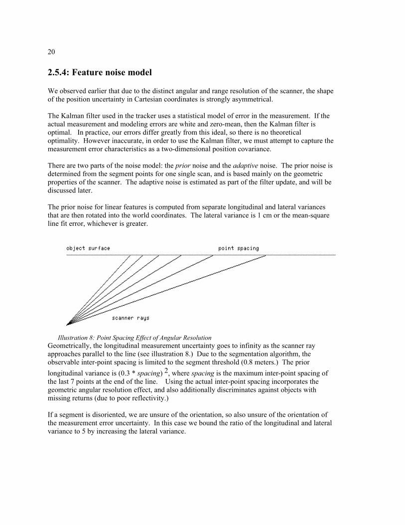
The prior noise for linear features is computed from separate longitudinal and lateral variances that are then rotated into the world coordinates. The lateral variance is 1 cm or the mean-square line fit error, whichever is greater.

Geometrically, the longitudinal measurement uncertainty goes to infinity as the scanner ray approaches parallel to the line (see illustration 8.) Due to the segmentation algorithm, the observable inter-point spacing is limited to the segment threshold (0.8 meters.) The prior longitudinal variance is (0.3 * spacing) 2, where spacing is the maximum inter-point spacing of the last 7 points at the end of the line. Using the actual inter-point spacing incorporates the geometric angular resolution effect, and also additionally discriminates against objects with missing returns (due to poor reflectivity.)

If a segment is disoriented, we are unsure of the orientation, so also unsure of the orientation of the measurement error uncertainty. In this case we bound the ratio of the longitudinal and lateral variance to 5 by increasing the lateral variance.

Illustration 8: Point Spacing Effect of Angular Resolution

21

Vague Line Ends

A line-end feature can be marked as vague, which means that its longitudinal position is so poorly determined that the endpoint position should be regarded as arbitrary by the tracker. A vague line end is still usefully localized laterally, and one end of a line can be vague when the other end isn't.

Due to shape change and occlusion, it turns out to be crucial to identify situations where the position of line ends is unreliable. This need results in a rather complex decision rule. A line end is vague if:1. The scanner point defining the endpoint position was occluded, 2. The prior longitudinal error estimate is exceeds 15 cm, or 3. The next adjacent point not assigned to this segment is at least 1.2 meters behind the line.

Any intervening no-return points are skipped.

Rule 3 has these functions:• It is a more precise occluded test in the case of a line with known orientation.• It also marks ends as vague when the adjacent point in the next segment falls near the same

line, hence may well be part of the same object that happened to be segmented separately due to missing returns.

Noise Adaptation

We make use of measurement noise adaptation to estimate the position covariance for each feature. The primary benefit of measurement noise adaptation is in its effect on the data-fusion aspect of the Kalman filter: noisy features contribute less to the motion estimate. This is valuable because some features are much noisier than others.

The noise is estimated from the statistics of the measurement residue, which is the disagreement between the predicted feature position and the measured one. (With our dynamic model, the residue is the same as the feature position innovation.)

The covariance of the residue is an estimate of the position measurement covariance.In theory, for computing an adaptive measurement noise, we should reduce the noise residue by the estimate covariance to represent the contribution to the measurement residue from the estimate uncertainty. However, this risks creating small or even negative measurement noise when the estimate covariance is too high. Since we are knowingly inflating process and measurement noise to deal with time-varying behavior and modeling error, this subtracting out the state covariance would to cause problems.

If the mean of the residue is not nearly zero, this indicates a non-zero-mean error. In some applications it would be appropriate to subtract out this mean from the measurement, but it our case, there is no independent measurement of the feature position, so a significant mean error means that we are not tracking properly. If the residue mean exceeds 10 cm, we reset the feature position from the current measurement and clear the residue mean to zero.

The need for this resetting comes from a sort of instability that the noise-adaptive tracker exhibits in the presence of time-varying non-zero-mean disturbances. In short, if a feature position drifts around, and no compensating track velocity is inferred (perhaps due to data fusion correctly

22

rejecting spurious motion), then the measurement covariance for that feature becomes inflated, and this further degrades the tracking performance for that feature. Our response in this situation is to allow the feature to be basically ignored by fusion, but to keep the feature position approximately correct by resetting the position when the residue mean becomes too large.

Residue update has two phases: during track startup, we compute recursive mean and covariance with equal sample weighting. After 0.3 seconds, we switch to a first order response (exponential decay) with 0.3 second time constant. Initially, the sample is small, so the estimate is unreliable. For the first 15 cycles, we use only the prior noise estimate. After 15 cycles, we use the sum of the residue covariance and (prior noise * 0.57). The prior noise then serves as a lower bound on the adaptive noise. This lower bound is particularly valuable in cases where there prior noise is high (like vague line ends.)

2.5.5: Information Increment Test

When attempting data association of a segment and track, we find the information increment, which is a measure of how much the track was influenced by this measurement. If the information increment is low, then the track is not responding to the measurement because the measurement is considered too noisy relative to how certain we think we are of the current state. In this case, the tracker is not actually tracking anything, just speculating based on past data.

A common problem situation is that a track may change to a line with both ends vague. In this case, the track is localized in one direction only, and the longitudinal velocity is unmeasured, which can lead to unacceptable spurious velocities. Low information increment can also happen if we reset all of the features in a track or when a track is very noisy (via noise adaptation.)

To keep the track from coasting indefinitely, we fail the association when the information increment is below 0.04 (response time constant of 25 cycles.) Tracks that are not associated for 10 cycles are deleted. If there is a one-to-one overlap relationship, then we pretend not to associate for purposes of the deletion test, but actually do associate. This helps to keep good tracks tracking properly in situations where the association is clear but the information is momentarily bad.

Though we call this "information" increment, the computation is really based on the covariance. This mimics the computation of the Kalman gain, which is what actually determines the response speed of the filter. If w+ is an eigenvalue of the covariance after the measurement, and w- is the eigenvalue before update, then the info increment is the mean of w- /w+ - 1 for the two eigenvalues. The eigenvalues are sorted so that we compare eigenvalues of similar magnitude.

The assumption is that the eigenvectors are little changed by any one measurement cycle, so the change in the sorted eigenvalues represents the change in uncertainty on each axis in the rotated (uncorrelated) coordinates. This insures that the track is well localized in two dimensions.

2.5.6: Improving the Kalman Filter for Outliers

The Kalman filter is optimal when the measurement error and process disturbance are Gaussian. One of the characteristics of the Gaussian is its light tails: it is very unlikely that a result will be very far from the mean. Unfortunately, when feature tracking breaks down, it can produce

23

outlier measurements which are effectively impossible in the Gaussian model.

A Kalman filter doesn't suppress these glitches, but it is common to extend the Kalman filter by entirely ignoring or limiting the magnitude of outlier measurements. We make use of this approach in several places:• If the change in track state due to a measurement is too incredible, then we discard the

measurement. This is done when the Mahalanobis distance of the state change exceeds 6. Before discarding the measurement, we see if we can get a reasonable association by resetting a subset of the features. We reset any features that contribute a state change with Mahalanobis > 4 by setting their position to the measurement, zeroing their contribution to the innovation.

• The time rate of change (d/dt) of velocity , acceleration and angular velocity are limited to physically plausible values: 9.8 meters/sec^2, 5 meters/sec^3, 60 degrees/sec^2. Note that these limits are applied to the incremental state change, not just to the output estimate. For example, the acceleration limit is applied not only to the acceleration estimate, but more importantly, also to the change in velocity estimate on any given update cycle. This prevents unreasonable jumps in position from causing big velocity jumps.

• The measurement of heading from feature orientation (orientation theta) is prone to jump when there is a track merge/split or the shape classification changes. If the innovation exceeds 7 degrees in this situation, then we reset the position to the new measurement.

2.5.7: Track Startup

When a track is newly created, the dynamics are unknown, so we assume that the velocity and acceleration are zero. If a track splits off of an existing track, we initialize the velocity and acceleration to the one for the existing track, but still leave the estimate covariance at the default (large) value.

Commonly tracks will come into range already rapidly moving, so this prior velocity can be significantly in error. It takes some time for the measurement to settle to the correct value, and dv/dt limiting prolongs this. During dv/dt limiting we hold acceleration fixed, as otherwise the acceleration slews wildly because the Kalman filter feedback loop is open. We also modify the Kalman filter update so that the velocity covariance is effectively fixed, preventing spurious covariance convergence.

The physical dv/dt limit does not apply during track startup because this velocity change is not a physical acceleration. As a heuristic, we increase the dv/dt limit when the velocity covariance is high. We allow the velocity to change by 12 sigmas per second if this is higher than the physical limit.

2.6: Track ValidationThe tracker outputs two flags for each track to aid in the interpretation of the result:

valid true when the motion estimate is believed to be accuratemoving true if there is compelling evidence that the track is moving

A track is considered apparently moving if it has a feature that has been tracked for at least 15 cycles, the speed is greater than 0.75 meters/sec and the Mahalanobis distance of the velocity from zero exceeds 6 sigmas. There is hysteresis in this test so that tracks tend to stay moving

24

once they are initially moving. Also, if a track is a line with two vague ends that was not previously moving, then only the lateral component of the velocity is considered.

If we use only this simple test, an unacceptable number of false motion detections result. Spurious velocities on fixed objects can easily cause false collision warnings. Since true imminent collisions are very rare, and fixed objects are very common, we must drive down the reporting of false velocities on fixed objects to a very low level in order to get an acceptable rate of false alarms.

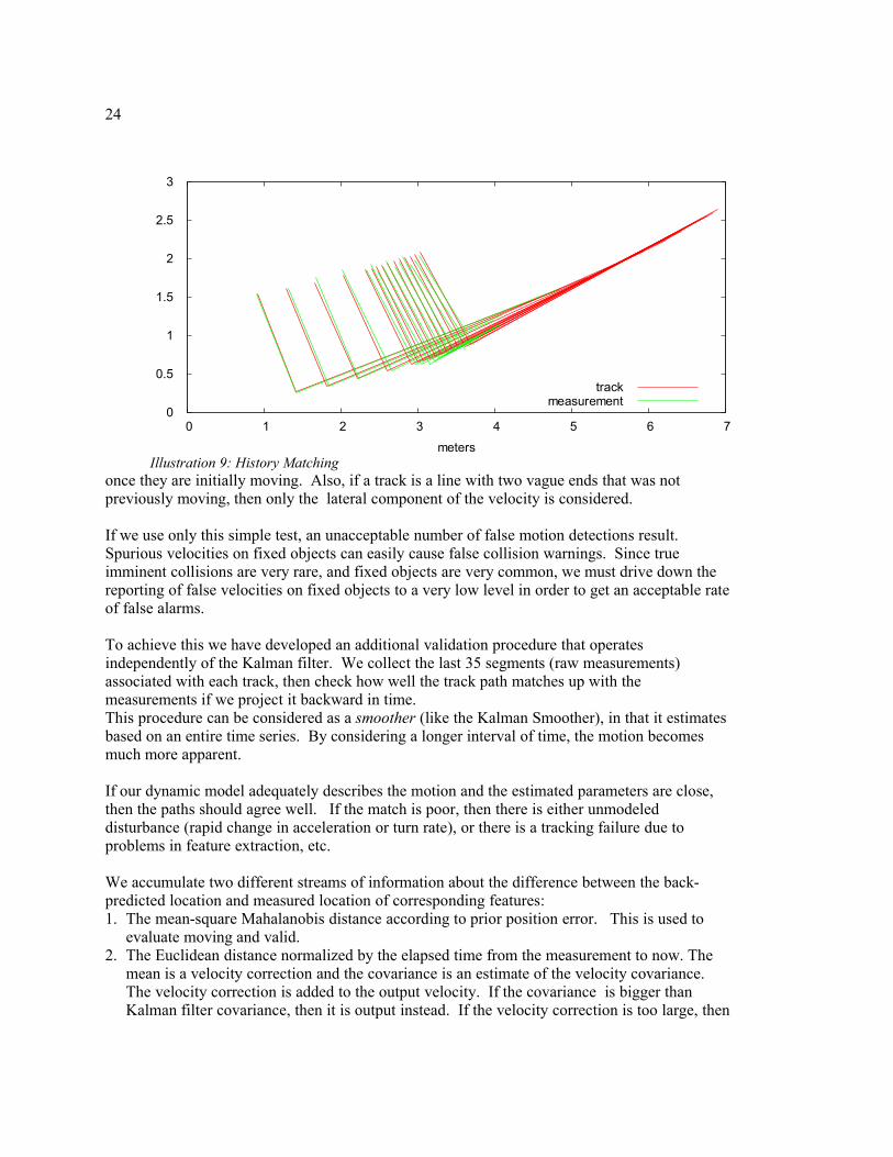
To achieve this we have developed an additional validation procedure that operates independently of the Kalman filter. We collect the last 35 segments (raw measurements) associated with each track, then check how well the track path matches up with the measurements if we project it backward in time.This procedure can be considered as a smoother (like the Kalman Smoother), in that it estimates based on an entire time series. By considering a longer interval of time, the motion becomes much more apparent.

If our dynamic model adequately describes the motion and the estimated parameters are close, then the paths should agree well. If the match is poor, then there is either unmodeled disturbance (rapid change in acceleration or turn rate), or there is a tracking failure due to problems in feature extraction, etc.

We accumulate two different streams of information about the difference between the back-predicted location and measured location of corresponding features:1. The mean-square Mahalanobis distance according to prior position error. This is used to

evaluate moving and valid. 2. The Euclidean distance normalized by the elapsed time from the measurement to now. The

mean is a velocity correction and the covariance is an estimate of the velocity covariance. The velocity correction is added to the output velocity. If the covariance is bigger than Kalman filter covariance, then it is output instead. If the velocity correction is too large, then

Illustration 9: History Matching

0

0.5

1

1.5

2

2.5

3

0 1 2 3 4 5 6 7

met

ers

meters

trackmeasurement

25

this is evidence of a tracking problem. In this case we don't apply the correction, and leave the track invalid.

We also find the sum of the position information for all features in the history that contributed to the distance estimate. This is used to determine whether the history has adequate quality to localize the track in two dimensions. The smaller eigenvalue of the information matrix must be greater than 35 meters-1.

This information eigenvalue is also used to normalize the Mahalanobis distance back into a nominal length, which is then thresholded for the moving/valid test. For a track to be marked valid, the distance must be less than 5 cm, and after that must stay below 15cm to remain valid. Though the units are meters, the physical interpretation is obscure. The empirically chosen values seem reasonable if regarded as an RMS fit error in meters. The advantage of this distance measure over a simple RMS distance is that it takes into consideration the asymmetric prior error distributions generated by the position measurement model.

We also compare the past measurements to the null hypothesis that we are not moving at all. This is done using the same comparison procedure, but with no projected motion. We then compare the matching error of the two hypotheses. For the track to be moving and valid, the matching error of the moving hypothesis must be 4 times less than that of the fixed hypothesis. This rejects situations where there is equal evidence for moving and non-moving because one feature moves and another doesn't.

In order to minimize the effect of noisy variation, the results of the history analysis are filtered using an order 21 median filter before being tested against the above limits.

Because the history-based validation is fairly computationally expensive (about 250 microseconds per track), we have used several optimizations:1. Only do history test on apparently moving tracks. When the validation is done, the track

must still be “apparently moving” after the velocity correction is applied to be considered moving.

2. Only use the oldest 1/3 of the history data, as this contains most of the information about velocity error.

3. Limit the number of tracks validated on any tracker cycle to 4. There are seldom this many moving tracks, so this limit is rarely exceeded. The purpose is to bound the runtime of a single tracker iteration.

2.7: Total Occlusion DetectionIf a track is totally occluded then the fact that we did not associate it on the current iteration is at best weak evidence that the object no longer exists. What we do is allow totally occluded tracks significantly longer to live without any associated measurement than we do for visible tracks (4 sec as opposed to 0.2 sec.)

We detect tracks that are totally occluded by looking at each previously partially occluded track which has not been associated and seeing if all of the points associated with that track at the last association are behind some visible object. We update the point position

26

by the last motion estimate, then test for visibility when seen from the POV of all scanners. Tracks are moved back to normal (non-occluded) status when all of the old points should now be visible in some scanner. This test is somewhat liberal, since in theory the object should be visible as soon as one point is visible again, but this makes up for changes in velocity during occlusion, etc.

27

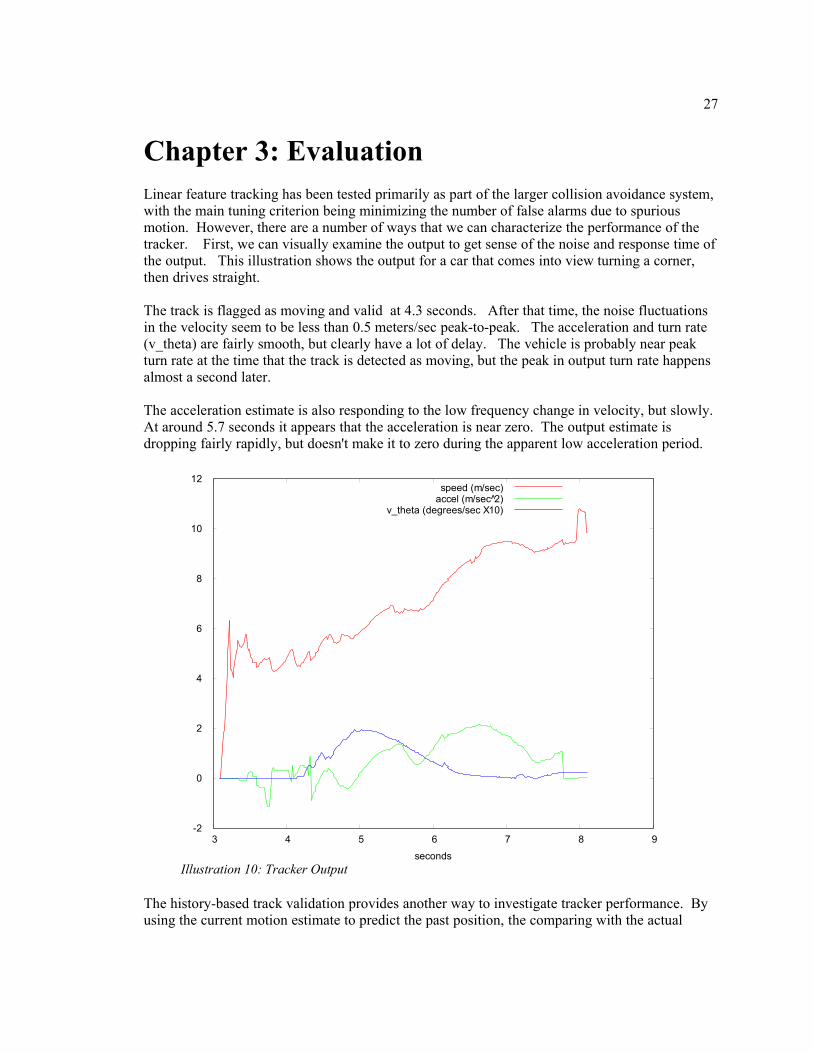
Chapter 3: EvaluationLinear feature tracking has been tested primarily as part of the larger collision avoidance system, with the main tuning criterion being minimizing the number of false alarms due to spurious motion. However, there are a number of ways that we can characterize the performance of the tracker. First, we can visually examine the output to get sense of the noise and response time of the output. This illustration shows the output for a car that comes into view turning a corner, then drives straight.

The track is flagged as moving and valid at 4.3 seconds. After that time, the noise fluctuations in the velocity seem to be less than 0.5 meters/sec peak-to-peak. The acceleration and turn rate (v_theta) are fairly smooth, but clearly have a lot of delay. The vehicle is probably near peak turn rate at the time that the track is detected as moving, but the peak in output turn rate happens almost a second later.

The acceleration estimate is also responding to the low frequency change in velocity, but slowly. At around 5.7 seconds it appears that the acceleration is near zero. The output estimate is dropping fairly rapidly, but doesn't make it to zero during the apparent low acceleration period.

The history-based track validation provides another way to investigate tracker performance. By using the current motion estimate to predict the past position, the comparing with the actual

Illustration 10: Tracker Output

-2

0

2

4

6

8

10

12

3 4 5 6 7 8 9

met

ers

seconds

speed (m/sec)accel (m/sec 2̂)

v_theta (degrees/sec X10)

28

measurements, we can get a sense of how well the tracker can predict motion over short periods of time (0.3 seconds)

3.1: Tracker prediction error vs. time horizonWhen we use the current motion estimate to predict the track position into the future, we expect that the quality of the match between the prediction and the actual measurement will degrade. This does not directly evaluate the accuracy of the of the track motion estimation, but rather the combined effect of estimation inaccuracy and any failing of the constant-acceleration constant-turn-rate model to capture the actual time-varying behavior of the tracked object.

To do this measurement, we use the linear features extracted from the raw scan at the future time and find the RMS distance between the predicted feature position and the measured one. Unfortunately, over the longer time horizons the features may not correspond that well. The tracker itself has considerable internal mechanism to suppress the effects of bad feature correspondences, but this simple evaluation procedure does not. Hence I believe that occasional large prediction errors are probably more due to a failure of this evaluation procedure, rather than actual prediction error.

Be that as it may, in this next plot, we can see the expected pattern where prediction error degrades with time horizon. This plot suggests that prediction is good at 1 second, but dicey at 5 seconds. As noted above, true performance may be somewhat better, but this does roughly correspond with other estimations that e.g. Christoph has done of vehicle motion predictability.

Illustration 11: Estimated Prediction Error

3.2: Sensitivity of Track validation ParametersHow well does the track validation (motion test) procedure work, and what is the parameter sensitivity? We analyzed a minute of data taken in a busy urban environment with numerous people and vehicles in it (illustration 12.) We visually determined from video and scanner data whether objects where truly moving or not if they were identified as moving prior to the history-based moving test. The tracks were then classified as truly moving if they corresponded to a car

29

or person that appeared to be moving, and false positive if they corresponded to some other object. This is classification is shown in bar 1.

Then we applied the moving test, using several different sets of sensitivity parameters. In condition 2 we are most willing to believe that tracks are moving, in 5 least willing. The blue or "false negative" are tracks that were correctly identified as moving at higher sensitivity settings, but at the lowest sensitivity are marked non-moving.

In this graph, clearly the incidence of false positive motion reports is greatly reduced, and at moderate parameter settings good results can be achieved with minimal increase in false negatives.

Illustration 12: Moving Test Performance

This validation procedure does not measure all false negatives, only those that introduced by the history-based moving test. The history motion test is only applied to tracks that have:

1. Mahalanobis distance of velocity estimate from zero > 6 sigmas 2. Magnitude of velocity estimate > 0.75 meters/sec.

Especially when the actual velocity is low, the estimated velocity may fall below this lower limit (when the true velocity is above), causing the track to falsely never be considered in the moving test.

30

Chapter 4: Unfinished WorkA number of ideas were not completely implemented or were in earlier stages of design exploration when code development stopped.

4.1: Time SkewA problem that confounds the recognition of object shape is that all the points on an object are not measured simultaneously. This problem is not too acute as long as nearby points are measured at nearly the same time, however this assumption does not hold when scans are interleaved (as the Sick does in 0.5 degree mode), or when multiple scanners with overlapping fields of view are used. The trunk code ignores this problem and uses the time of the last point in each scan as the time for all of the measurements in the scan.

Because of the interaction with multiple scanners, the SCANNER_FUSION branch has code which corrects for time skew. Time skew is corrected for by finding the mean measurement time for each segment, then adjusting the positions of each point according to the estimated track velocity and the time skew between the point measurement time and the mean track time. Of course, this correction can't be made until after data association, so we must compensate the points and refit the rectangle model after association.

4.2: Multiple ScannersOriginally, partly for CPU load sharing, multi-scanner tracking was implemented by running separate trackers for each scanner. Because of this assumption, we exploited the single scanner perspective to improve efficiency, especially by assuming that the inherent azimuth ordering in the scanner output is also an ordering of consecutive points on the object surface.

However, when there is substantial overlap in the scanner fields of view some fusion of multiple scanners is needed so that tracks won't be duplicated. This is currently supported by processing each scanner output separately, effectively fusing the scanner data at the segment level. This works fairly well, but often causes tracks to break up when they should be handed off from one scanner to the next, and causes a lot of spurious apparent measurement noise when an object is visible in more than one scanner, because we repeatedly sequentially associate the same track with different views of the same object. The appearance fluctuation problem must be handled before it is possible to evaluate tracks for time-consistency in appearance.

The SCANNER_FUSION CVS branch contains a first cut at a different approach to multi-scanner fusion, which is to fuse tracks at the point cloud level, before segmentation. This is clearly a better way to do things, but unfortunately runs into some sticky implementation difficulties, primarily because of places in the code where a single-scanner point of view was implicitly assumed.

For one thing, with multiple scanners, it is common to see three sides of an object, and in general one might see all four. So the limited two-side model no longer works. Secondarily, some use is made of the assumption that there is a natural “topological” ordering of the scan points, where

31

consecutive points on the surface of a single object are consecutive in the point ordering. This assumption makes it much more tractable to detect gaps in objects and to determine which side of an object a point belongs to. This effectively reduces 2D problems into 1D problems. Unfortunately, there is in general no globally consistent 1D ordering of points when there are multiple scanners. For example, when multiple scanners see several objects from opposite sides, the objects may appear in a different order in different scans.

The SCANNER_FUSION code attempts to create locally consistent orderings for individual segments, which is usually possible, but this has considerable complexities which have not been satisfactorily resolved. One problem arises when two scanners see opposite sides of a thin surface. It may make more sense to fit this as a single line, but the new code may end up fitting as three sides of a rectangle, when ensuing confusion due to the lack of a full 4-side model. Note that if we do fit as a single line, then the point orderings may be opposite from the POV of the different scanners.

Of course, it is also only possible to find a proper topological ordering of the points on the surface when the object has no holes in it. In practice this is probably not a big deal, as one of the main purposes is to make it easier to detect holes.

To make SCANNER_FUSION work right it would probably be necessary to generalize the segment/track model to a full 4-sided rectangle, and this should probably be combined with a revamp of simple segmentation to make it well integrated with model-based segmentation. For example, model-based segmentation could assign points to the sides, instead of the corner detection currently used. But some form of non-model-based fitting would still be needed for new tracks.

4.3: Track classification based on shape/textureWe investigated ways of classifying objects by their shape or texture that can be used in addition to the current test based on fitting a rectangular model. We were primarily interested in recognizing objects such as foliage or ground returns which are hard to track successfully, causing false motion detections, however this could be part of a more general classification framework that identifies objects more specifically as pedestrian, car, building, etc.

The idea was to somehow capture the judgment of a human looking at scan data that bad tracks such as vegetation look “noisy”.

We first investigated classifying based on the spectrum of the object appearance, treating the mismatch between the measured surface and a line fit as a 1D signal. To convert the 2D shape into a 1D signal, we find the mismatch between each point and the rectangle model, effectively unwrapping the sides of the rectangle to generate a pseudo time-series. The scan data is irregularly spaced, so it was interpolated onto fixed distance intervals.

32

The results of frequency-domain analysis are somewhat discouraging.

Although there is clear difference between the spectra, there is not much new information not given by the RMS line match error and object size. In particular, though the amount of energy below the 0.5 meter scale varies considerably, the general shape of the spectra show similar high frequency rolloffs. This means that there is not much information not already present in the line match error amplitude.

Basically, there is not enough information in an individual scan to classify a track. The subjective impression of noise seems to relate to apparent inconsistency of shape between scans.

4.4: Time ConsistencyThe main tool that we have for discriminating between good tracks and garbage is the consistency of the track over time. Track validation evaluates the consistency of the motion over time (though more could possibly be done there in evaluating the “purposefulness” of the motion, e.g. is there net motion.)

Another form of consistency is the consistency in the appearance over time. Adaptive feature noise does get at this to some degree because if the outline fluctuates a lot, this will increase the feature position noise, but this information is not taken into account for track validation or classification.

4.4.1: Shape constancyWe investigated aligning multiple scans of the same object and examining the degree of similarity to characterize whether the object has stable structure beyond the first-order linear fit. The data was one-dimensionalized and resampled as for the frequency domain analysis, and then the scans for individual tracks were were aligned according to maximum cross correlation.

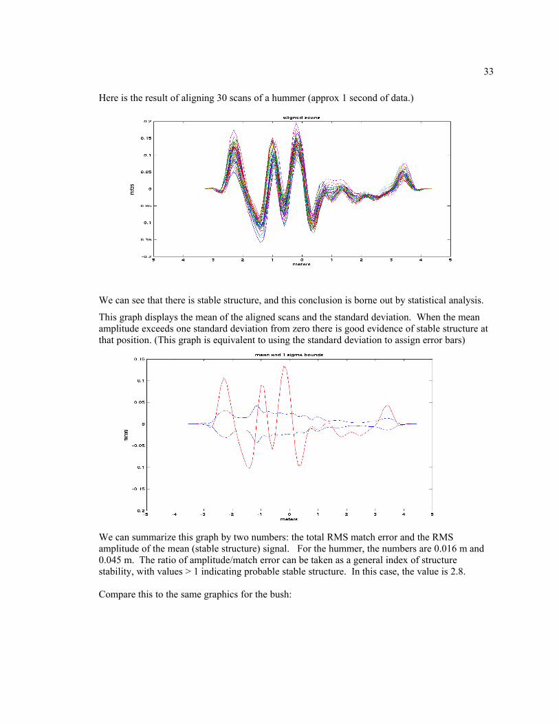
33

Here is the result of aligning 30 scans of a hummer (approx 1 second of data.)

We can see that there is stable structure, and this conclusion is borne out by statistical analysis.

This graph displays the mean of the aligned scans and the standard deviation. When the mean amplitude exceeds one standard deviation from zero there is good evidence of stable structure at that position. (This graph is equivalent to using the standard deviation to assign error bars)

We can summarize this graph by two numbers: the total RMS match error and the RMS amplitude of the mean (stable structure) signal. For the hummer, the numbers are 0.016 m and 0.045 m. The ratio of amplitude/match error can be taken as a general index of structure stability, with values > 1 indicating probable stable structure. In this case, the value is 2.8.

Compare this to the same graphics for the bush:

34

We can see that the scans are much more dissimilar, and there is no significant stable structure. The match error is 0.02 and the structure amplitude is 0.001, giving a stable structure index of 0.05. For these two cases, the stable structure index varies by a factor of 56, strongly distinguishing the two cases.

The amount of stable structure as determined by this approach would clearly be a valuable input to a general classifier.

4.5: General ClassificationReliability would be increased and value would be added if there was a general classifier which classified tracks based on various generalized numeric features. This could consider shape consistency over time, motion consistency, size, speed of motion, etc.

35

4.6: Improved EstimationThere is definitely room for more sophisticated motion estimation, especially with respect to rotational estimation. I find the Segmenting Track Identifier [Linder01, Schell04] particularly promising. This approach tries to match circular arcs onto the recorded path, and has been shown to work better than most other algorithms on realistic data of unpredictably maneuvering tracks such as fish and bats. As presented it is computationally untraceable, though, but some simplified version that didn't require general nonlinear optimization might be useful.

Another approach would be to generalize the track validation velocity correction into a full velocity/turn estimate, perhaps by using a Kalman smoother, which the current velocity correction can be considered a variant of.

In general, with a better path-based estimator of whatever kind, it might then be profitable to drop turn and acceleration estimation out of the basic Kalman filter, relying on the general block estimator that is only applied to apparently moving tracks to extract the higher-order motion.

36

Bibliography

[MacLachlan06] R. MacLachlan, C. Mertz, “Tracking of Moving Objects from a Moving Vehicle Using a Scanning Laser Rangefinder”, Intelligent Transportation Systems 2006, IEEE proceedings

[MacQueen67] J. B. MacQueen (1967): "Some Methods for classification and Analysis of Multivariate Observations, Proceedings of 5-th Berkeley Symposium on Mathematical Statistics and Probability", Berkeley, University of California Press, 1:281-297

[Schell04] Schell, Chad, Stephen Paul Linder and James R. Zeidler (2004) Tracking Highly Maneuverable Targets with Unknown Behavior. Special Issue of the Proceedings of the IEEE on Sequential State Estimation: From Kalman Filters to Particle Filters, 92:3, pp. 558 - 574.

[Linder01] Linder, S.P. , Ryan, M.D., and Quintin, R.J. (2001) Concise Track Characterization of Maneuvering Targets. AIAA Conference on Guidance, Navigation, and Control Conference. Montreal, CA.

37