Embed Size (px)
Citation preview
Atmos. Meas. Tech., 6, 1659–1671, 2013www.atmos-meas-tech.net/6/1659/2013/doi:10.5194/amt-6-1659-2013© Author(s) 2013. CC Attribution 3.0 License.
EGU Journal Logos (RGB)
Advances in Geosciences
Open A
ccess
Natural Hazards and Earth System
Sciences
Open A
ccess
Annales Geophysicae
Open A
ccess
Nonlinear Processes in Geophysics
Open A
ccess
Atmospheric Chemistry
and Physics
Open A
ccess
Atmospheric Chemistry
and Physics
Open A
ccess
Discussions
Atmospheric Measurement
TechniquesO
pen Access
Atmospheric Measurement
Techniques
Open A
ccess
Discussions
Biogeosciences
Open A
ccess
Open A
ccess
BiogeosciencesDiscussions
Climate of the Past
Open A
ccess
Open A
ccess
Climate of the Past
Discussions
Earth System Dynamics
Open A
ccess
Open A
ccess
Earth System Dynamics
Discussions
GeoscientificInstrumentation
Methods andData Systems
Open A
ccess
GeoscientificInstrumentation
Methods andData Systems
Open A
ccess
Discussions
GeoscientificModel Development
Open A
ccess
Open A
ccess
GeoscientificModel Development
Discussions
Hydrology and Earth System
Sciences
Open A
ccess
Hydrology and Earth System
Sciences
Open A
ccess
Discussions
Ocean Science
Open A
ccess
Open A
ccess
Ocean ScienceDiscussions
Solid Earth
Open A
ccess
Open A
ccess
Solid EarthDiscussions
The Cryosphere
Open A
ccess
Open A
ccess
The CryosphereDiscussions
Natural Hazards and Earth System
Sciences
Open A
ccess
Discussions
Tracking isotopic signatures of CO2 at the high altitude siteJungfraujoch with laser spectroscopy: analytical improvementsand representative results
P. Sturm1,*, B. Tuzson1, S. Henne1, and L. Emmenegger1
1Empa, Swiss Federal Laboratories for Materials Science and Technology, Laboratory for AirPollution and Environmental Technology,Uberlandstrasse 129, 8600 Dubendorf, Switzerland* now at: Tofwerk AG, Uttigenstrasse 22, 3600 Thun, Switzerland
Correspondence to:B. Tuzson ([email protected])
Received: 21 December 2012 – Published in Atmos. Meas. Tech. Discuss.: 15 January 2013Revised: 5 June 2013 – Accepted: 10 June 2013 – Published: 12 July 2013
Abstract. We present the continuous data record of atmo-spheric CO2 isotopes measured by laser absorption spec-troscopy for an almost four year period at the High Alti-tude Research Station Jungfraujoch (3580 m a.s.l.), Switzer-land. The mean annual cycles derived from data of Decem-ber 2008 to September 2012 exhibit peak-to-peak amplitudesof 11.0 µmolmol−1 for CO2, 0.60 ‰ for δ13C and 0.81 ‰for δ18O. The high temporal resolution of the measurementsalso allow us to capture variations on hourly and diurnaltimescales. For CO2 the mean diurnal peak-to-peak ampli-tude is about 1 µmolmol−1 in spring, autumn and winter andabout 2 µmolmol−1 in summer. The mean diurnal variabil-ity in the isotope ratios is largest during the summer monthstoo, with an amplitude of about 0.1 ‰ both in theδ13C andδ18O, and a smaller or no discernible diurnal cycle during theother seasons. The day-to-day variability, however, is muchlarger and depends on the origin of the air masses arrivingat Jungfraujoch. Backward Lagrangian particle dispersionmodel simulations revealed a close link between air compo-sition and prevailing transport regimes and could be used toexplain part of the observed variability in terms of transporthistory and influence region. A footprint clustering showedsignificantly different wintertime CO2, δ13C andδ18O val-ues depending on the origin and surface residence times ofthe air masses.
Several major updates on the instrument and the cali-bration procedures were performed in order to further im-prove the data quality. We describe the new measurementand calibration setup in detail and demonstrate the en-hanced performance of the analyzer. A measurement preci-
sion of about 0.02 ‰ for both isotope ratios has been ob-tained for an averaging time of 10 min, while the accuracywas estimated to be 0.1 ‰, including the uncertainty of thecalibration gases.
1 Introduction
Isotopes are ideal tracers of sources and sinks of carbon diox-ide (CO2). They provide unique information on the fluxesof CO2 between the different pools involved in the carboncycle. This is because the physical, chemical and biologicalexchange processes slightly fractionate between the differentisotopes leading to characteristic isotopic signatures in theatmosphere, land and ocean. The carbon isotope composi-tion of CO2 (δ13C) is an excellent marker, for example, forpartitioning oceanic and biospheric fluxes (Ciais et al., 1995;Keeling et al., 2011). Interpreting variations in the oxygenisotope composition of CO2 (δ18O) is more challenging be-cause theδ18O is affected by both the carbon and water cy-cles (Farquhar et al., 1993). However, theδ18O has been usedto estimate gross biosphere fluxes (Ciais et al., 1997; Welpet al., 2011).
Stable isotope measurements traditionally rely on flasksampling and isotope ratio mass spectrometry (IRMS),reaching precisions forδ13C and δ18O in CO2 of about0.01 and 0.02 ‰, respectively (Werner et al., 2001). Anovel alternative approach for measuring isotope ratios islaser spectroscopy. This optical technique allows for in situmeasurements with high time resolution (up to 10 Hz), and
Published by Copernicus Publications on behalf of the European Geosciences Union.

1660 P. Sturm et al.: Tracking isotopic signatures of CO2 at Jungfraujoch with laser spectroscopy
precisions up to 0.02 ‰ have been reached forδ13C of atmo-spheric CO2 (Richter et al., 2009). In addition to dedicatedresearch instruments (Tuzson et al., 2008b; Richter et al.,2009), several commercial CO2 isotope analyzers have be-come available in the last decade. A tunable diode laser ab-sorption spectrometer using a liquid nitrogen cooled lead-salt laser enabled the study of isotopic carbon fluxes interrestrial ecosystems (Bowling et al., 2003, 2005; Griffiset al., 2004, 2008). Other recent commercial instruments arebased on cavity ring-down spectroscopy (Vogel et al., 2012),off-axis integrated cavity output spectroscopy (McAlexan-der et al., 2011), or quantum cascade laser absorption spec-troscopy (Sturm et al., 2012). Another optical technique isbased on Fourier transform infrared spectroscopy (Griffithet al., 2012).
Despite these analytical advancements, long-term mea-surements of tropospheric CO2 isotopes using laser spec-troscopy have not yet been reported. The goals for inter-laboratory compatibility defined by the World Meteorolog-ical Organization (WMO) are 0.01 ‰ forδ13C and 0.05 ‰for δ18O (WMO, 2011), which is very challenging indepen-dently of the technique used. Therefore, characterizing andimproving the performance of CO2 isotope analyzers is stillessential, in particular when applied to monitoring of atmo-spheric background air.
Here we present our continuous data record of CO2 iso-topes measured by laser spectroscopy at the High AltitudeResearch Station Jungfraujoch, Switzerland, from Decem-ber 2008 to September 2012. At this station, biweekly flasksampling and the analysis of the CO2 isotopic compositionby mass spectrometry started in 2000 (Sturm et al., 2005;van der Laan-Luijkx et al., 2012). Since December 2008, astate-of-the-art quantum cascade laser absorption spectrom-eter has also been deployed for continuous (1 Hz) in situmeasurements of the isotopic composition of carbon dioxide(Tuzson et al., 2011). Based on the experiences gained fromthese measurements, several major updates on the instrumentand the calibration procedures were performed in order tofurther improve the data quality. We describe our new mea-surement and calibration setup including the required dataprocessing steps, show the performance of the improved an-alyzer and illustrate the capability of this method with repre-sentative results. Finally, backward Lagrangian particle dis-persion simulations are used to distinguish the origin of theair masses arriving at Jungfraujoch and to establish a rela-tionship between the potential source and sink regions andthe observations.
2 Methods
2.1 Measurement site
The High Altitude Research Station Jungfraujoch (JFJ,7◦59′ E, 46◦33′ N) is located on a mountain saddle on the
northern ridge of the Swiss Alps at an altitude of 3580 mabove sea level (Sphinx Observatory). The station is mostlysituated in the free troposphere, but intermittently influencedby polluted planetary boundary layer (PBL) air reachingthe site during synoptical uplifting or convection (Zellwegeret al., 2003). The mean atmospheric pressure is 654 hPa andthe mean annual temperature is−7.5◦C. Because of the highelevation, the year-round accessibility and the special geo-graphical situation in the center of Europe the site is wellsuited for long-term monitoring of tropospheric backgroundair but also for studying the transport of anthropogenic orbiogenic tracers from the boundary layer to the free tropo-sphere. A large number of trace gases and aerosol parametersare routinely monitored at Jungfraujoch as part of the SwissNational Air Pollution Monitoring Network (NABEL) andthe Global Atmosphere Watch (GAW) programme of WMO.
2.2 Instrument setup
The quantum cascade laser absorption spectrometer em-ployed for the CO2 isotope monitoring was developed atEmpa in collaboration with Aerodyne Research Inc. in 2007and was presented in detail inNelson et al.(2008) andTuz-son et al.(2008a). The instrument was first used for fieldstudies near sources (Kammer et al., 2011; Tuzson et al.,2008a) and has been then deployed at Jungfraujoch (Tuzsonet al., 2011). Briefly, the laser spectrometer uses a thermo-electrically cooled pulsed quantum cascade laser emitting at4.3 µm. The instrument is based on differential absorptionspectroscopy with two identical optical paths and a pair ofmultipass absorption cells with a path length of 7.3 m each tosimultaneously analyze sample and reference gas. The laseremission frequency is scanned over the absorption lines ofthe three main CO2 isotopologues12C16O2, 13C16O2 and18O12C16O and the transmitted light is recorded with ther-moelectrically cooled infrared detectors (PVI-3TE-4.4, VigoSystems, Poland). A dedicated, commercially available soft-ware (TDLWintel, Aerodyne Research Inc., USA) is used forspectral analysis. The laser temperature and voltage, the celltemperature and pressure as well as the automatic calibra-tions including data processing into preliminary calibratedvalues are controlled using custom written LabVIEW code.
Sample air is drawn from the heated NABEL main inletfrom the roof of the Sphinx laboratory. The sampling setupfrom December 2008 to November 2011 was as described inTuzson et al.(2011) with a sample pump upstream of the in-strument and four solenoid valves for calibration. This pumpwas removed in November 2011 as it had a small leak due toa damaged diaphragm, and from then on the sample air wasdrawn through the instrument by the pump downstream ofthe measurement cell only.
In this work we present analytical improvements and rel-evant new developments that we found necessary for long-term and reliable monitoring. In March 2012, i.e., after morethan three years of spectroscopic measurement at the remote
Atmos. Meas. Tech., 6, 1659–1671, 2013 www.atmos-meas-tech.net/6/1659/2013/

P. Sturm et al.: Tracking isotopic signatures of CO2 at Jungfraujoch with laser spectroscopy 1661
MFC 2
MFC 1Temperaturestabilization
Reference cell
Pump
Sample cellWorking standard 1/2
Drift standard
Reference gas
Highflow
Compressor CO2 / H2O Adsorber Ascarite
Purge air foroptics
MFC 3
Temperaturestabilization
MFC4
Working standard 3
Primary standards 1-4
Sampleinlet
Pump
Nafion dryer
12-port
Spare inlet
Fig. 1.Gas handling setup.
site Jungfraujoch, several hardware components were up-graded and a new calibration and gas-handling setup wasimplemented (Fig.1). In the newly developed gas handlingmodule, a 12-port multi-position valve (EMT2SD12MWE,VICI AG International, Switzerland) selects between thesample air stream and one of several primary and work-ing standard gases. The sample cell flow rate is about350 mLmin−1. The reference cell is constantly flushed withcompressed air from a cylinder at a flow rate of about50 mLmin−1. Both gas flows are temperature controlled andpreheated to match the optical module temperature whenentering into the multipass cells. The gas pressures in thereference and sample cell are measured by absolute pres-sure manometers and actively controlled at 80± 0.003 hPaby adjusting the set points of two mass flow controllers(MFC2022, Axetris AG, Switzerland). Zero air is generatedby an oil-free reciprocating air compressor and a carbondioxide absorber/dryer (MCA1, Twin Tower Engineering,USA). Zero air is used to purge the optics housing at a flowrate of 1 Lmin−1 and occasionally to stepwise dilute a stan-dard gas with a mass flow controller in order to correct forconcentration dependence of the isotope ratios. The temper-ature stability of the optics was improved by adding furtherthermal insulation around the optical module and by usingmore precise PID (proportional-integral-derivative) temper-ature controllers (3216, Eurotherm Produkte AG, Switzer-land). Thus, variations of the gas temperature in the mea-surement cells are typically damped by a factor of 100 com-pared to the laboratory air temperature variations (i.e., a 1 Kchange in the laboratory temperature results in a∼ 10 mKchange in the cell temperature). The stability of the cell tem-perature is typically about±5 mK over 24 h. Furthermore,the set point resolution of the laser temperature controller(LFI3751, Wavelength Electronics, USA) was enhanced bysupplying an external voltage signal to the analogue inputof the controller. This overcomes the limitations set by thedigital-to-analog converter of the temperature controller and
allows a much tighter control of the laser frequency and thuseliminates any spectral drift. Finally, the power supply of thelaser driver was replaced by a low-noise device (PWS4323,Tektronix Inc., USA).
2.3 Calibration and data processing
The calibration procedure up to March 2012 was as de-scribed inTuzson et al.(2011). Briefly, a drift standard wasmeasured every 15 min, one calibration standard was mea-sured every two hours and another calibration standard every12 h. Each calibration gas was sampled for 300 s, except thedrift standard, which was sampled for 128 s. Whenever anyof the calibration standards was nearly empty, a new cali-bration cylinder with the same CO2 concentration and iso-topic composition was prepared and analyzed against the oldstandard cylinders, an in-house NOAA-ESRL standard (fromNOAA Earth System Research Laboratory/Central Calibra-tion Laboratory, USA, with the isotope composition ana-lyzed by INSTAAR at the University of Colorado, USA)and occasionally against other calibrated standard gases. TheCO2 mole fraction of the calibration gases was measured bygas chromatography and since 2010 with a cavity ring-downspectrometer (G1301, Picarro Inc., USA) and linked to theWMO-X2007 scale using in-house NOAA-ESRL standards.
In spring 2012, an improved calibration strategy was im-plemented. A set of four primary standards was prepared(Table 1). Three standards were produced by mixing dif-ferent amounts of CO2 from different sources (marine car-bonate; PanGas AG, Switzerland, and methane burning;Messer Schweiz AG, Switzerland) into aluminium cylin-ders and then diluted with synthetic air (79.5 % N2, 20.5 %O2). A fourth cylinder with aδ18O value closer to the at-mosphericδ18O contains compressed air (Messer SchweizAG, Switzerland). Subsamples of these gases were filled into1.5 L glass flasks and the isotopic composition relative to theVPDB-CO2 standard was determined by isotope ratio mass
www.atmos-meas-tech.net/6/1659/2013/ Atmos. Meas. Tech., 6, 1659–1671, 2013

1662 P. Sturm et al.: Tracking isotopic signatures of CO2 at Jungfraujoch with laser spectroscopy
Table 1.Primary standards with the assigned values on the WMO-X2007 scale for CO2 and the VPDB-CO2 scale forδ13C andδ18Oas determined in spring 2012.
CO2(µmol δ13C δ18O
Tank no. Mixture mol−1) (‰) (‰)
CB08984 CO2 + syn. air 383.40 −3.54 −14.11CB08970 CO2 + syn. air 394.43 −8.00 −17.38CB08999 CO2 + syn. air 388.36 −12.01 −20.523076 compressed air 429.06−10.57 −7.65
spectrometry in the WMO Central Calibration Laboratory atthe Max-Planck-Institute for Biogeochemistry (MPI-BGC),Jena, Germany. The CO2 mole fraction was linked to theWMO-X2007 scale by our NOAA-ESRL standards usingthe cavity ring-down spectrometer. The primary standardsare expected to last for> 20 yr and our calibration scalesare linked to these four gases. Three shorter-lived secondaryworking standards are then used to calibrate the instrument.These working standards are measured against the primarystandards at Jungfraujoch about every two months to estab-lish the working standard scale and to check for drifts in theworking standard cylinders. They have a lifetime of about1 yr and are replaced when the cylinder pressure decreasesto below 30 bar. All calibration gases are stored in 30 L alu-minium cylinders (Scott-Marrin, Inc., USA), except for oneprimary standard consisting of compressed air, which is a20 L stainless steel cylinder. The reference and drift gasesare contained in 50 L stainless steel cylinders. The regulatorsare two-stage high-purity brass regulators (412 Series, CON-COA, Pangas AG, Switzerland) and all tubing is either stain-less steel tubing or Synflex tubing (SERTOflex 1300, SertoAG, Switzerland).
The new calibration procedure is as follows: every 30 mina drift cylinder (compressed air) is measured for 5 min. Thethree working standards are analyzed every 6 h for 5 mineach. Two working standards are used to perform a two-pointcalibration for the CO2 mole fraction and the isotope ratios.The third standard is treated as a target cylinder to check thestability of the working standard calibration. One workingstandard with a high CO2 mole fraction is also used to mea-sure every 5 days the concentration dependence of the iso-topes by diluting it with zero air.
The isotopologue mole fractions based on spectral fittingrequire several data post-processing steps to obtain calibrateddata. The processing procedure for the isotope ratios of thepre-March-2012 data consists of the following steps. First,a drift correction due to changes in gas temperature, laserfrequency shifts, laser intensity fluctuations and gas pres-sure is applied. A multiple linear regression of the drift stan-dard measurements with the four previously mentioned in-strument parameters is performed to remove the influence of
changing instrument parameters on the isotope ratios. Themagnitude of this correction was typically 0–3 ‰, while thecontribution of the influencing parameters varied from caseto case. Since the relationship between the isotope ratios andone of the instrument parameters can change when there isa change in the system setup (i.e., new reference gas cylin-der, stepwise adjustment of the laser frequency, change inthe fitting parameters, etc.), raw data are analyzed in blockswith constant conditions. This lead to blocks of data spanningfrom a few days to a few weeks that were analyzed consecu-tively. A smoothing spline is applied to the residual variationsstill present in the corrected drift standard measurements andused to remove this remaining scatter from the sample andcalibration measurements. The next step is the concentra-tion dependence correction of the isotope ratios. Finally, theactual calibration is performed using one of the calibrationstandard measurements. For most of the 2009–2011 time pe-riod a one-point (offset) calibration is applied. The instru-ment response (slope of measured CO2 versus WMO scaleor measured isotope ratios versus VPDB-CO2 scale, respec-tively) was determined from manual calibrations performedwith different calibration gases and assumed to remain con-stant. This turned out to be the more robust calibration ap-proach compared to using a 2-point calibration, because theuncertainty of the calculated calibration slope was larger thanthe real variations in the slope coefficients. Furthermore, datacould also be calibrated in a consistent way at times whenthere was only one calibration gas available.
The improvements in the instrument stability implementedin spring 2012 allowed for a simplification of the data pro-cessing. In particular, the drift correction based on corre-lations with instrument parameters is obsolete. Instead, thedrift standard measurements (every 30 min) are used in afirst step to remove any drift. Next, the concentration de-pendence correction is applied. Third, the calibration coeffi-cients (slope and offset) are calculated based on the 6-hourlycalibration measurements. To further reduce the uncertaintyin the calibration coefficients a smoothing spline is fitted tothese values. The smoothed calibration coefficients are thenapplied to the sample data to get calibrated values. Finally,the 1 s data are averaged to 10 min mean values.
2.4 Transport simulations and footprint clustering
The Lagrangian particle dispersion model (LPDM) FLEX-PART (Version 9.0) (Stohl et al., 2005) was used in back-ward mode to calculate source sensitivities for Jungfraujochfor the whole observation period. At each 3-hourly inter-val, 50 000 model particles were initialized at the locationof Jungfraujoch and traced back in time for 10 days. FLEX-PART considers horizontal and vertical displacements due tothe mean atmospheric flow, turbulent mixing especially inthe atmospheric boundary layer and vertical transport dueto deep convection. Here, the model was driven by Euro-pean Centre for Medium Range Weather Forecast (ECMWF)
Atmos. Meas. Tech., 6, 1659–1671, 2013 www.atmos-meas-tech.net/6/1659/2013/
P. Sturm et al.: Tracking isotopic signatures of CO2 at Jungfraujoch with laser spectroscopy 1663
operational analysis (00:00, 06:00, 12:00 and 18:00 UTC)and +3 h forecasts (03:00, 09:00, 15:00 and 21:00 UTC) with91 vertical levels and a horizontal resolution of 0.2◦
× 0.2◦
for the Alpine area (4◦ W–16◦ E, 39◦–51◦ N) and 1◦ × 1◦ forthe global domain. The limited horizontal resolution of themodel does not represent well the Alpine topography and,hence, a large difference between observatory and model alti-tude exists. In previous studies, the optimal release height forJungfraujoch was determined to be at 3000 m above sea level,almost halfway between the real station’s altitude and themodel ground (Keller et al., 2011; Brunner et al., 2012). Weadopted this initial altitude in the current study as well. Thesimulated source sensitivities can directly be multiplied withmass releases at a source grid cell, yielding simulated molefractions at the receptor (Seibert and Frank, 2004). Sourcesensitivities are given in units s m3 kg−1 and are also referredto as residence times or footprints. Source sensitivities weregenerated on a regular grid of 0.1◦
× 0.1◦ covering Europeand a secondary grid of 0.5◦
× 0.5◦ horizontal resolution forthe Northern Hemisphere. The lowest vertical output levelreached up to 100 m above model ground, which is the sameas the minimal mixing height in the model.
In order to distinguish different transport regimes towardsJungfraujoch, source sensitivities were used in a clusteringmethod. A straightforward clustering approach would be totreat the simulated source sensitivities in every grid cell asan individual variable in a cluster analysis. The number ofcluster variables would then be equal to the number of gridcells in the output grid and quickly become too large to beefficiently handled by any cluster algorithm. Hence, a reduc-tion of the cluster variables is required. This can be achievedby aggregating grid cells with small average residence timesto larger grid cells, a procedure also used in regional scaleinversion studies (Keller et al., 2011; Vollmer et al., 2009).Starting from grid cells with 0.1◦ resolution, we allowed ag-gregation to grid cells with up to 3.2◦ horizontal resolution,if the total residence time in the aggregated cells remainedbelow a certain threshold. This threshold was iteratively de-duced so that the total number of aggregated grid cells didnot exceed 100. Only the European output domain was con-sidered for the clustering, which will focus the separation offlow regimes more onto the regional scale transport and to alesser degree onto inter-continental transport.
The clustering was performed on the time series of res-idence times of the aggregated surface grid cells only.Since these variables were not normally or log-normally dis-tributed, we chose an alternative distance measure to obtainthe dissimilarity matrix,D with elementsdi,j , that is used inthe clustering process. Absolute distances between the ranksof the surface sensitivities over time were calculated accord-ing to
di,j =
N∑k=1
∣∣rank(τk)i − rank(τk)j∣∣ , (1)
where the source sensitivities are indicated asτ and the in-dex k runs over all aggregated grid cellsN , while i andj refer to the time. The matrixD is symmetric and con-tains zeros in the diagonal. The off-diagonal elements con-tain the distance between two transport simulations at dif-ferent times. Finally, based on the dissimilarity matrix theclustering was calculated using k-medoids clustering (Kauf-man and Rousseeuw, 1990), which was previously success-fully used for cluster analysis of single trajectory simula-tions (Henne et al., 2008). The number of selected clusterswas obtained using the silhouette technique (Kaufman andRousseeuw, 1990) by choosing the number of clusters (inthe range 2 to 20) for which the average silhouette widthsshowed a local maximal. In the present case, a local max-imum was obtained for 8 clusters with an average silhou-ette width of 0.16. A similar technique for clustering sourcesensitivities as obtained from LPDM calculations was pre-sented byHirdman et al.(2010). However, they aggregatedresidence times to larger regions defined by continental orcountry borders and Euclidean distances between these wereused to derive the dissimilarity matrix.
To display the different flow regimes, average residencetime maps per cluster were generated by summation over allcluster members and division by the number of clusters. Forall clusters these show maximal values close to the site. Inorder to emphasize the differences between the individualclusters, the difference of cluster average and overall averageresidence times was computed and normalized by the meanof cluster and overall average (residence times by cluster nor-malized: RTCN). In this way, differences can be displayed ina linear and symmetric fashion, with RTCN values rangingfrom −2 to 2. Areas with RTCN larger than 0 indicate areaswith greater than average surface contact and values largerthan 1 indicate areas with 3 times larger residence times.
3 Results and discussion
3.1 Precision
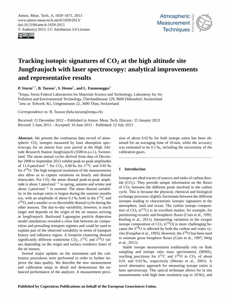
The precision and stability of the updated instrument wascharacterized by the two-sample standard deviation (Werleet al., 1993) and is shown in Fig.2. Tank air with a CO2 molefraction of 401 µmolmol−1 was continuously measured onsite for 5 h. The two-sample standard deviation with 1 s dataacquisition is compared with the initial performance mea-surements reported byTuzson et al.(2008a). The most sig-nificant improvement compared to our previously reportedvalues is the extended white-noise dominated region allow-ing for substantially longer averaging times (∼ 10 times).The better operation stability reduces the requirements forfrequent calibrations and thus minimizes the calibration gasconsumption, which is of crucial importance for long-termmonitoring. In addition, a lower instrumental drift is ben-eficial for the data post-processing, e.g., corrections and
www.atmos-meas-tech.net/6/1659/2013/ Atmos. Meas. Tech., 6, 1659–1671, 2013

1664 P. Sturm et al.: Tracking isotopic signatures of CO2 at Jungfraujoch with laser spectroscopy
0.01
2
4
68
0.1
2
4
68
1
Two
sam
ple
stan
dard
dev
iatio
n (‰
)
1 10 100 1000Averaging time (s)
0.01
2
4
68
0.1
2
4
68
1
1 10 100 1000
δ13CTuzson et al. (2008) this work
δ18OTuzson et al. (2008) this work
Δtopt = 695 s Δtopt = 840 s
Fig. 2. Two-sample standard deviation (Allan deviation) of cylin-der air measurements forδ13C andδ18O. The stability performanceof the upgraded instrument (colored markers) is compared with thevalues reported for this spectrometer byTuzson et al.(2008a) (graymarkers). The slight degradation in precision at 1 s averaging time islargely compensated by the higher stability at longer timescales (asindicated by1topt). The optimum averaging time (topt) is reachedafter∼ 12 min for both isotope ratios, corresponding to an analyt-ical precision of 0.02 ‰. The white and drift noise influenced do-mains are indicated by gray and colored dashed lines.
calibrations. This stability improvement is a result of thebetter temperature, pressure and laser frequency control. Asa consequence, the interval for the drift standard measure-ments was increased from 15 to 30 min. The precision of theCO2 mole fraction measurement is 0.16 µmolmol−1 at 1 sand 0.01 µmolmol−1 at 10 min averaging time. The best pre-cision of about 0.02 ‰ is reached for an averaging time ofabout 10 min for both isotope ratios.
The half hourly cylinder air measurements are still wellcorrelated with the laboratory temperature (correlation coef-ficients of 0.6 to 0.8 for CO2 andδ13C and−0.4 to−0.7 forδ18O). Thus, temperature variations remain the major sourcefor the drift on timescales longer than about 15 min, althoughit is not clear whether this is due to optical or electronic com-ponents that may both respond to temperature fluctuations.
A more detailed comparison of the precision before andafter the instrument upgrades is shown in Fig.3. It shouldbe noted that the instrument has been running for more thantwo years almost unattended and without major revisionsleading to some reduction in performance. During the se-lected time period of six days in June 2011 and June 2012the CO2 mole fraction was relatively constant between 390and 396 µmolmol−1 and consequently the variations in theisotope ratios are small. The lower noise level in the 10 minaveraged data for June 2012 is obvious and demonstratesthe benefits of the instrument upgrades. Averaging to hourlymean values (solid lines in Fig.3) greatly reduces the noise,in particular for the data before the upgrade. This is signifi-cant because data of background monitoring sites are usuallyreported as hourly mean values or even aggregated to longerintervals when compared with model output (e.g., fromFLEXPART, see Sect.3.4).
●●●
●●
●
●●
●●●
●●
●●
●
●
●●●●●●
●●●
●●●●●●●●●●
●●●
●●●●●
●●●●●●●●●●●●●●●●●●●●●●●●●●●●
●●●●●●●●●●●●
●●●●●●
●●●●●●●●●●●●●●●●●●●●●●●●●●●●●●●●●●●●●
●●●
●●●●
●●
●
●●●
●●
●
●●●●●●
●●●●●●●●●●●●●
●●●
●
●●
●
●●●●●
●●●●●●●●●●●●●●●●●●●●●●●●●●●●●●●●●●●●●●●●●●●●●
●●●
●●●●●●
●●●●●
●
●●●●
●
●
●●●●●●●●
●
●●●●●●●●●●●●
●●●
●●●●●●●●
●
●
●●●●●●●
●●●●●●●●●●●●●●●●●●●●●●●●●●
●●●●●●●●●●●●●●●●
●●●●●●●●●●●●●●●●●●●●●
●●●●
●●
●●●●●●●●●●●●●●●●●●
●●
●
●●●●●●●●
●●●●●●●●●
●●●●●●
●●●
●●●●●●
●●
●●●●●●●●●
●●●●●●●●●●●●●●●●●●●●●●●●●●●●●●●●●●●●●●●●●●●●●●●●●●●●●●●●●●●●●●●●●●●●●●●●●●●●●
●
●●●●●●●
●●●
●●●●●●
●●●
●
●●●●
●●●●●●●●●●●●●●●●●●●●●●●●
●●●●●●●●●●●●●●●●●●●●●●●●●●●●●●●●●●●●●●●●
●●●●●●●●●●●●●
●●●●●
●●
●
●●
●
●●
●●●●●●●●●●●●●●●●●●●●●
●●●●●
●●●
●
●●●●●●
●
●
●●●●●●●●●●●●●●●
●●●●●●●●●●●●●●●
388
390
392
394
396
CO
2 (µ
mol
mol
−1)
●●●
●
●●●●●
●
●
●
●
●
●
●●
●●
●
●
●
●●
●
●
●
●●●
●
●
●
●
●
●
●
●
●●●
●
●●
●
●
●
●●
●●●
●●
●
●
●
●●
●●
●
●
●●
●
●
●
●
●
●●
●
●
●
●
●
●
●
●
●
●
●
●
●
●
●
●
●
●
●
●
●
●●
●
●●●
●
●
●
●
●
●●
●
●
●
●
●
●●
●●
●
●
●
●
●
●●
●
●●
●
●
●
●
●
●●●
●
●
●
●
●
●
●
●
●
●
●●
●
●
●
●●
●
●●
●
●●
●●
●●
●●
●
●
●●
●
●
●
●
●
●
●
●
●
●●
●
●●
●
●
●●
●
●
●●●
●●
●
●
●
●
●
●●
●
●
●
●
●
●
●
●
●
●
●
●
●
●●●●●●●
●
●
●
●
●
●
●
●
●
●
●
●
●
●
●
●●●●
●
●
●
●
●
●
●●
●●
●
●
●●●●●
●
●●●
●
●
●
●
●
●
●●
●
●
●
●
●●
●●
●
●
●
●
●
●
●●
●
●
●
●
●
●
●
●
●
●
●
●
●
●●●●
●●●
●
●
●
●●
●
●
●
●
●●●●
●●
●●●
●
●
●
●
●●
●
●
●
●
●
●
●
●●
●
●
●●
●
●
●
●
●
●
●
●
●
●
●
●
●
●
●
●●●
●
●●
●●
●
●
●
●
●●
●
●●
●
●
●●
●
●●
●
●
●
●
●
●
●
●
●
●
●
●●
●
●●
●
●●
●●●●
●
●
●
●●●
●
●●●
●
●
●
●
●
●●
●
●
●●
●
●
●
●
●
●
●●
●●
●
●●●
●
●
●●
●
●
●
●
●
●
●
●
●
●●
●
●
●
●
●●
●
●
●
●●
●
●
●
●●
●●
●
●
●●
●
●
●●
●●
●
●
●
●●●
●
●●
●
●●●●
●
●
●
●
●
●●
●
●
●
●●●
●
●
●
●
●
●
●
●●
●
●●
●
●●
●
●●
●
●
●
●
●
●
●
●
●
●
●●
●
●
●
●
●
●
●
●●
●
●●
●
●●
●
●●
●
●●
●●
●
●
●
●
●●
●
●
●
●
●●
●
●●
●●
●
●
●
●
●
●
●
●
●
●
●
●●
●
●●
●
●
●
●
●●
●
●
●
●
●
●●●
●
●
●
●
●
●●
●
●●
●
●●
●
●
●
●
●●
●●
●
●
●
●
●
●
●
●
●●
●
●
●
●●
●
●
●●
●
●
●
●
●
●
●●
●
●
●
●●
●●
●
●
●
●
●
●
●●
●●
●
●
●
−9.0−8.8−8.6−8.4−8.2−8.0
δ13C
(‰
)
●
●
●●
●●
●
●
●●
●●
●
●
●
●●
●●
●
●
●●
●●
●
●
●●●
●●●
●
●
●
●
●●●●
●●●●
●●
●
●●
●
●●
●
●
●
●
●●
●●●
●●●
●
●
●●
●
●●
●
●
●●
●
●
●
●●●
●
●●
●●
●
●
●●
●
●
●
●
●
●
●
●
●
●
●●
●
●
●
●
●
●
●●
●
●
●
●●●
●●
●
●
●
●
●●●●●
●●
●
●
●
●
●●
●
●
●
●●●
●
●●
●
●
●
●
●
●
●
●
●
●●
●
●
●
●
●
●
●
●●
●
●
●
●
●
●
●●●
●
●
●
●
●
●
●
●
●
●
●●
●
●
●
●
●
●●●
●
●
●●
●●
●
●●
●
●
●
●
●
●
●
●
●
●●●
●●●●
●
●
●
●
●
●
●●●
●●
●●
●
●
●●●
●●●●
●
●
●
●●
●
●
●
●●
●●
●●
●
●
●
●●●
●
●
●●
●
●●
●●●
●
●●
●
●
●
●
●
●●
●
●
●●
●
●
●●
●
●●
●●
●
●
●
●
●●
●
●●●
●
●●
●
●
●
●
●
●
●
●●
●●
●
●●●
●
●
●
●
●
●
●
●
●●
●
●●
●
●
●
●
●●●●●●
●
●
●
●●
●●
●●
●●
●●
●
●
●●
●
●
●
●
●
●●
●
●
●
●
●●
●
●
●●
●
●
●
●
●●●
●
●●●●
●
●●
●
●●
●●
●
●
●●
●
●
●●
●
●
●●
●
●
●
●●
●
●
●
●●●
●●●●
●●●
●
●
●
●
●●
●
●
●
●
●
●
●
●●
●
●
●
●
●
●
●
●
●
●
●
●●●●
●
●●
●●
●
●
●
●
●
●
●
●●
●
●●●
●
●●
●
●
●
●
●
●
●●
●
●
●
●
●
●
●
●●
●
●
●
●●
●●
●
●●
●
●
●
●
●●
●
●
●
●●
●
●●●
●●●
●●
●
●
●
●
●
●
●●
●
●
●
●
●
●●
●●
●
●
●
●
●
●
●
●
●
●
●●
●
●
●
●●
●
●
●●
●
●●●
●
●
●
●
●
●
●●
●●●
●●●
●●
●●●
●
●
●●
●
●
●
●
●
●
●●●
●
●
●
●●●
●
●
●
●
●
●●
●
●
●●
●
●
●
●
●
●●
●
●●
●
●
●
●
●
●●
●
●
●
●
●
●
●
●
●●
●
●●
●●
●
●
●●
●●
●
●
●
●
●
●
●●●
●●
●
●
●
●
●
●●
−0.4−0.2
0.00.20.40.60.8
δ18O
(‰
)
20−Jun 22−Jun 24−Jun
2011
●●●●●
●●●●●
●●●
●
●●●●●●●●●●●●●●●●●●●●
●●
●●
●●●●●●
●●●
●
●●
●●●
●●●
●●●
●●
●●●●
●
●●
●
●
●●
●●
●
●●●
●
●
●●●●
●●●●●●●●●
●●●●●●●●●
●●●●●●●●●●●●●●●●
●
●●●●●
●●●
●●●●●●
●
●
●●●●●●●●
●●●●●●●●●●●●●
●●●●●●●●●●●●●
●●●●●●●●●●
●●●
●●●●●●●●●●●●●●●●●●●●●
●●●●●●●●●●●●●●●●●●●●●●●●●●●●●●●●●●●●●●●●●●●●●●●●●●●●●
●
●●
●
●
●
●●●
●
●●●●
●●
●
●
●
●
●●●
●●
●
●●
●●
●●●
●●●
●
●
●
●
●●●●●●●●
●●●●●●●
●●●
●●●●
●●●●●●●●●●●●●●●●●●●●●
●●●●●
●
●
●●●●
●●
●●●
●●●●
●●●●●●●●●●●●●●
●●●●●●●●●●●●●
●●●
●
●●●●●
●
●●●●●
●
●●●
●
●
●●●
●
●●
●
●
●
●
●●●●●●
●●
●●●●●●●●●●●●●●
●●●●●●
●
●●●●●●●●●
●●●●●●●●
●●●●●●
●●●●●●
●●●●●●●●●●
●●●●●●●●●
●●●●●●●●●●●●●●●
●●●●●●●●●●●●●●●●
●●●
●
●●
●●●●
●
●
●
●●●●●●
●●
●●
●
●●●●●●
●●●●●●●●●●●●●●
●●●●●●●
●
●●●●●●●●●●●●●
●●●
●●●●
●●
●
●●
●●●
●●●●●●
●●●
●
●●●
●
●●●●●
●●●
●●●●●●●●●●●●
●●●
●●●●●
●●●●●●●●●●●
●●●
●
●
●●
●●
●
●
●
●●
●
●
●
●
●●
●
●
●
●●
●●●●
●
●
●
●●
●
●
●
●
●
●
●●
●
●●●
●
●
●●●●
●●
●
●
●
●●
●●
●
●
●
●●●
●
●●
●●
●●●●
●●
●●
●
388
390
392
394
396
CO
2 (µ
mol
mol
−1)
●●●●
●●●●
●
●●
●●
●
●●●
●●●●
●●●●●
●●●●●●
●●●●
●●
●●●●●
●
●
●●●●●
●
●●●●●●●●●●●●●●●●●●●●●●●
●●
●●●●●●●●●
●●
●
●●●●●
●
●●●●●●
●●●●●
●
●●●●●●
●●●
●●●●●●●●●
●●●●
●●●●●●●●●
●●
●
●
●●●●●
●
●●●●●●●
●●●●
●●
●●
●●●●●●●●●●●●●●
●●●●
●●●●●●●●●●●●●
●
●
●●
●●
●
●
●●
●●●●●
●●●●●●●●●●●●●
●●●●
●
●●
●
●●
●●●●●●●
●
●●●●●●●●●●●
●
●●●●●
●●●●●
●●●●●●●
●
●●●
●
●●●●●●
●●
●●●●●●
●●●●●●
●
●●
●●●●●
●
●
●●●●
●●●
●●●●●●
●●●●●●●●
●●●●●●●●●●●●●●●●●●●●●●
●
●●
●●●●
●●●
●●●●●●
●●
●●●●●●
●
●●●●●●
●●●●
●●●
●●
●
●●●●●●
●●●
●●●●●
●●●●●●●●●
●
●
●
●●
●●
●
●●
●●●
●
●●●●●
●
●●●●●●
●
●
●●●●●
●●●●●●●
●
●
●●●●●
●
●●●●●●●●●
●●●●●●●●●
●●●
●
●●●
●●●●●●●●●●●●
●●
●●●●●●
●
●
●
●
●●●●●
●●●●●●●●
●●
●●●●●●
●
●●●●●●
●
●●
●●●●●●
●
●●
●●●●●●●●●
●●●
●●
●
●
●●●●●●
●●●●
●
●●
●
●●●●●
●●●●●●●●●●●●
●●●●●
●
●●●●
●
●
●●●●
●
●
●
●●●●
●●●●
●●●●●●●●
●●●●●●
●●●●●●
●
●
●●
●
●●●●●●●●●
●
●●
●
●●
●
●●●●●●●
●
●
●●●●●●●●
●●
●●
●●●●
●●●●●●●
●
●
●●
●
●●●
●●●
●●
●
●●
●●●
●●●●●
●●●
●●
●●●
●●●
●
●
●
●●●●●●●
−9.0−8.8−8.6−8.4−8.2−8.0
δ13C
(‰
)
●●●●●●●●●●●●●
●
●●●●●●●●●●●●●●●●●●●●●●●●
●●●
●
●
●●●●
●●●●●
●
●●●
●
●●●●
●●●●
●●●●●●●●●
●
●
●●
●
●
●●●
●●
●●
●
●●●●
●●
●●
●●●
●
●●
●
●
●
●
●●●●●●●●
●
●
●●●●●●●
●
●●●
●●●●●●●●●
●●●●
●
●●
●
●●
●
●●●
●●●●●●
●●●●●●●●●●●●●●●●●●●●●●●
●
●●●●●●●●●
●●●●
●
●●●●●
●
●
●●●●●●●
●●●●●●●●●●●●●●●
●●
●
●●●●●●●●●●●●●●●●●●●●●●●●
●●●●●●
●●●●●●
●
●●●
●
●●
●●●
●
●●●●●●●●●
●●
●●●●●●●●●
●
●●●●●●
●
●●●●●●●
●●
●●●●●
●●●
●●●●●●
●
●●●●
●
●●●●●●●●●●●
●●●
●
●●●●
●●●
●
●●●●●●
●●●●●●●●
●●●
●
●●●
●●●●●●●●●●●●
●
●●●●●●●●●●●●●●●●
●●●●●●●●
●
●
●
●●●
●
●●●●●
●
●●●●●
●
●●●
●●●
●
●
●
●●●●●●●●●●●
●●
●
●●●●●
●●●●●●●●●
●●
●
●●●●●
●
●●●
●●●
●●●●●●●●●●●●●●●●●●●●●
●
●●●●●●●●
●●●●●●●●
●●
●●●●●●
●
●●●●●
●
●●●●●●●●●
●
●●●●●●●●●●●
●●●
●●●
●
●●●●●
●
●●●●
●
●●●
●
●●●●
●●●●●●●●●●●●●●●
●●
●
●●
●
●●
●
●●●●●●●●●
●●
●●
●●●●●
●●●●●●●●●
●●
●
●●●
●
●●●●●●●●●●●●●●●
●
●●
●●●
●
●●●●●●●●●
●●●●●●●●●
●
●●
●●●
●●●●●●●●●
●●
●
●●●●●●
●●●●●●
●●●
●
●●●●
●●●
●●
●●●
●●
●
●
●●
●●●●●●
●
−0.4−0.2
0.00.20.40.60.8
δ18O
(‰
)
20−Jun 22−Jun 24−Jun
2012
Fig. 3. Comparison of 10 min averaged data for six days inJune 2011 and 2012, i.e., before and after the instrument upgrades.The solid lines are the 1 h averaged data.
Four months of target cylinder measurements after the in-strument upgrade are shown in Fig.4. The assigned valuesof the target cylinders have been determined using the pri-mary standards and the uncertainty ranges (±1σ ) are de-picted as shaded areas in Fig.4. Each single target cylindermeasurement consists of a 120 s average and the standarddeviation of the isotope ratio data of 0.06–0.07 ‰ roughlycorresponds to the measurement precision at 120 s averag-ing time (Fig.2). Analyzing the target cylinder for more than120 s would most likely lead to an even smaller spread inthe target cylinder data. However, there is a clear trade-offimplemented in our sampling/calibration strategy. The targetreference gas is measured for 5 min, but given the transitionand flushing time of the spectrometer, the first 3 min are dis-carded and only the last 2 min are considered for analysis. Al-though the measurement precision in this case is by a factor2.2 lower than the precision achievable using the optimumaveraging time defined by the Allan variance minimum, itis still within the uncertainty of our primary standards (seeFig. 5). A slight reduction of the scatter in the target gasdata (Fig.4) would only be possible at the expense of sig-nificantly more target gas consumption (13 min vs. 5 min),which would involve their replacement every 5 instead of 12months. We consider that the effort to produce, reference andtransport these calibration gases as well as to assure conti-nuity in the measurements outweighs the potential 0.02 ‰improvement in precision.
Figure5 shows the instrument response from the analysisof the four primary standards. The residuals of the linear fitbetween the measured and the assigned values indicate thelinearity and accuracy of the instrument. The standard devia-tion of the residuals from Fig.5 is 0.12 µmolmol−1 for CO2,0.06 ‰ for δ13C and 0.13 ‰ forδ18O, respectively, which
Atmos. Meas. Tech., 6, 1659–1671, 2013 www.atmos-meas-tech.net/6/1659/2013/

P. Sturm et al.: Tracking isotopic signatures of CO2 at Jungfraujoch with laser spectroscopy 1665
ooo
oo
o
o
oo
ooooo
oooooooo
oooooooooo
oo
o
oooooooooooooooo
oo
ooo
ooo
o
oooo
oooooo
o
ooooooooo
ooo
o
oooo ooo
o
oooo
oo
oooooooo
o
ooooooooo
ooooooo
o
ooooooooo
o
ooooooooooooooo
ooo
oo
oooo
oooo
oo
ooooo
oooooooooooooooooooo
o
ooooo
o
ooooooo
o
oooooooooooooooooooooooooooooo
oooo
ooo
o
oooo
o
oooooooooooooooo
ooo
o
ooooo
oo
ooooooo
o
o
o
o
o
ooooooooo
ooooooooooooooooo
ooo
oooooooo
ooooooooooooo
o
ooooooooooooooo
o
oooooooo
ooo
oooooooooooo
oo
oo
o
o
o
o
o
o
oo
oo
405.15
405.20
405.25
405.30
405.35
405.40
pos2.mean.new$date[msk]
CO
2 (µ
mol
mol
−1)
mean: 405.28SD: 0.03
o
oo
o
oooo
oooooooooo
o
ooooo
oo
o
ooooo
ooo
oooooooooooooooo
o
oo
ooo
o
ooooooooooooo
o
oooo
oo
ooooo
oooooo oo
oo
oooooo
oooooooooooooooo
oo
o
o
ooo
o
oooooooooooo
ooooooo
oooooo
o
o
oooooo
o
ooooooo
o
ooo
o
o
ooooooooo
o
o
o
oo
o
ooooooooo
o
oooooooo
oooooooooo
oooooo
oo
oo
oo
ooooo
ooooooooooooooooo
o
oo
oooo
o
o
ooooo
o
oooooo
o
oo
ooooo
ooooo
o
o
o
oooooo
oo
ooooooo
o
ooooo
ooooooooooooo
oooooooo
oooooooo
ooo
o
ooooo
ooo
o
oo
oooooooooooooooooooo
oooo
o
o
o
ooooo
o
oo
oo
o
o
oo
o
−11.4
−11.3
−11.2
−11.1
−11.0
−10.9
−10.8
pos9.mean.new$date[msk]
δ13C
(‰
)
mean: −11.08SD: 0.07
ooo
o
o
o
o
ooooo
ooooooooo
oooooooooooooo
o
oooooooooooooooooo
oooooo
o
ooo
o
oo
oooooooo
oooooooooo
ooo
oooooooooooooooo
ooooo
o
oooooo
oooo
ooooooo
o
ooooo
ooooooooo
o
oo
ooooo oo
ooooooo
oo
ooo
o
oooooo
oo
ooooo
o
ooooo
ooooo
o
oooo
o
ooooo
ooooo
ooooooooooo
o
o
o
oooooooooooo
oo
o
ooooo
oooooooo
oooooooooooooooooooo
o
oooooooo
oooooo
o
o
oooooooo
ooooooooooo
o
o
oooooooo
o
o
o
oooooooo
oo
oooo
ooo
o
o
oooooo
ooooooo
o
oooo
o
oo
ooooo
o
o
oooooo
oo
ooooooooooo
o
ooo
o
oooo
Jul Aug Sep Oct
−14.6
−14.5
−14.4
−14.3
−14.2
−14.1
−14.0
pos2.mean.new$date[msk]
δ18O
(‰
)
mean: −14.28SD: 0.06
Fig. 4. Target gas measurements during four months (June toSeptember 2012). The histograms show the distribution of the datawith the respective mean and standard deviation. The shaded areasare the assigned values with the uncertainty (1σ ) derived from theprimary standard calibrations.
are typical values for the measurement of the four primarystandards.
3.2 Long-term data record
An overview of the data record from December 2008 toSeptember 2012 is shown in Fig.6. Hourly averaged datafor CO2, δ13C andδ18O as well as fitted background curvesare plotted. Two different methods have been used to calcu-late the long-term background values. The first method de-composes the signal into a long-term trend, a yearly cycleand short-term variations (Thoning et al., 1989). This curvefit consists of a combination of a polynomial (second or-der) and annual harmonic (n = 4) functions and the resid-uals from this fit are then smoothed using a low pass filter(80 days cutoff). The second method uses local regression(60 days window) to extract the baseline signal (Ruckstuhlet al., 2012). This is a non-parametric and thus very flexibleapproach and accounts for a possibly asymmetric contami-nation of the background signal (e.g., in winter local pollu-tion always leads to a positive deviation from the backgroundCO2 concentration). The mean difference of the baseline val-ues between the local regression and the smoothed curvefit are−0.63± 0.55 µmolmol−1 for CO2, 0.04± 0.04 ‰ forδ13C and 0.06± 0.05 ‰ for δ18O, respectively. An ordinaryleast squares regression between the two baseline estimatesyields slopes of 1.054 (R2
= 0.98), 1.037 (R2= 0.97) and
1.024 (R2= 0.98) for CO2, δ13C andδ18O. Thus, both meth-
ods give very similar results and highlight the seasonal dy-namics of the carbon dioxide and its isotopic composition inthe atmosphere.
The gap in the time series in autumn 2011 was due to apump failure. The diaphragm of the sample pump, which wasoriginally installed upstream of the instrument, was broken.This resulted in a small leak and the influence of laboratory
air could be seen as a small increase in the CO2 mole fractionwhen people were present in the room. Data periods whenthe sample air was contaminated with laboratory air were re-moved based on a comparison with CO2 data from anothertrace gas analyzer (G2401, Picarro Inc., USA), which usesthe same air inlet. Data were flagged as contaminated bylab air, when the difference in the CO2 mole fraction ex-ceeded 2 µmolmol−1. This is a conservative limit with re-gard to the isotope ratios, which were also affected by thiscontamination. Assuming that the CO2 mole fraction in thewell ventilated lab increases from 400 to 1000 µmolmol−1
due to the presence of people in the laboratory and theδ13Cof the respired CO2 is −23 ‰ (Epstein and Zeiri, 1988), onewould expect aδ13C of the laboratory air of about−17 ‰(compared to−8 ‰ of the background CO2). A contribu-tion of 2 µmolmol−1 CO2 from laboratory air would then inturn lead to a change in the measuredδ13C of 0.045 ‰ at themost. This is less than the overall measurement uncertaintyat that time. Using this procedure, 8 % of the data were re-moved during the period with the leak. Additionally, from11 July to 16 September 2011 all data has been removedfrom further analysis because no CO2 data from the trace gasanalyzer was available during this period and as a result thedata could not be screened for contamination.
We compared our laser based data with IRMS values froman intercomparison programme ofδ13C flask measurements(van der Laan-Luijkx et al., 2012). These samples were takenat Jungfraujoch between December 2007 and August 2011and analyzed by three different IRMS laboratories. They re-vealed average differences between the laboratories of−0.02to −0.03 ‰. The standard deviation of the individual dif-ferences was between 0.20 and 0.30 ‰. They conclude thatthe WMO goal for the measurement compatibility ofδ13C(±0.01 ‰) (WMO, 2011) is not yet reached within this flasksampling program. If we compare our hourly averaged val-ues that correspond to the flask sampling times with the flaskresults from the MPI-BGC laboratory then the average differ-ence is−0.03 ‰ with a standard deviation of 0.19 ‰. Thisis similar to the differences between the flask samples andindicates that our data compare well with the flask data andwithin the inter-laboratory uncertainty of different isotope ra-tio mass spectrometry labs. Forδ18O, the average differenceto the MPI-BGC flask data is−0.31 ‰ with a standard devi-ation of 0.26 ‰ (W. Brand, personal communication, 2012).This substantial difference can be explained by the larger un-certainty in ourδ18O calibration scale, mainly because theδ18O value of our standard gases (−24 to −10 ‰) did notspan the range of the measuredδ18O values (∼ 0 ‰). Flaskdata for comparison are not yet available for the period sinceMarch 2012, but we expect that both the precision and the ac-curacy have been improved by the instrument and calibrationupgrades presented in this work. Nevertheless, continuing ef-forts are needed to evaluate the uncertainties and ensure thehigh accuracy and the traceability of the data, which are re-quired at background monitoring sites like Jungfraujoch.
www.atmos-meas-tech.net/6/1659/2013/ Atmos. Meas. Tech., 6, 1659–1671, 2013

1666 P. Sturm et al.: Tracking isotopic signatures of CO2 at Jungfraujoch with laser spectroscopy
●
●
●
●
●
●
●
●
400
410
420
430
440
CO2
[12C
O2]
●
●
●
●
●
●
●
●
●
●
●
●
●●
●
●
380 390 400 410 420 430
CO2 (µmol mol−1)
Res
idua
ls
−0.10.00.1
●
●
●
●
●
●
●
●
0.855
0.856
0.857
0.858
0.859
0.860
0.861
0.862
δ13C
[13C
O2]
/[12C
O2]
●
●
●
●
●
●
●
●
●●
●
●
●●
●
●
−12 −10 −8 −6 −4
δ13C (‰)
Res
idua
ls
●●
●
●
●●
●
●
−5e−50e+05e−5
●
●
●
●
●
●
●
●
0.930
0.932
0.934
0.936
0.938
0.940
0.942
δ18O
[C18
OO
]/[C
16O
O]
●
●
●
●
●
●
●
●
●
●
●
●
●
●
● ●
−20 −16 −12 −8
δ18O (‰)
Res
idua
ls
−1e−40e+01e−4
Fig. 5. Instrument response versus assigned values of the four primary standards as determined on 25 May 2012. The solid lines are weightedlinear least squares fits to the data. The residuals from the fit are shown in the lower panels with the error bars representing the standard errorof the mean. The ordinate represents the natural abundance weighted isotopologue ratios as retrieved by the spectrometer.
380
390
400
410
420
CO
2 (µ
mol
mol
−1)
−10.0
−9.5
−9.0
−8.5
−8.0
−7.5
δ13C
(‰
)
2009 2010 2011 2012
−2.0−1.5−1.0−0.5
0.00.51.0
Date
δ18O
(‰
)
Date
Fig. 6.Overview of the data record from December 2008 to Septem-ber 2012. Hourly averaged data of CO2 (red),δ13C (blue) andδ18O(green) as well as fitted background curves (black: local regression,gray: smooth curve fit, see text for explanation) are shown.
3.3 Mean seasonal and diurnal cycles
Mean annual cycles derived from the monthly bin-averageddata as well as from the annual harmonic part of the smoothcurve fit are shown in Fig.7. The averaged data have beendetrended using the long-term trend derived from the smoothcurve fit. The peak-to-peak amplitude of the seasonal vari-ation is 11.0 µmolmol−1 for CO2, 0.60 ‰ for δ13C and0.81 ‰ forδ18O. This is in good agreement with the season-ality obtained from independent flask measurements whereamplitudes of 10.54 µmolmol−1 for CO2 and 0.54 ‰ forδ13C have been observed for the period between Decem-ber 2007 and August 2011 (van der Laan-Luijkx et al., 2012).
The seasonality in CO2 andδ13C is dominated by the landbiosphere and the relative contribution of photosynthesis andrespiration (net ecosystem CO2 exchange). The minimum in
CO2 mole fraction in August nearly coincides with the max-imum in δ13C and is due to peak net ecosystem CO2 uptake.The CO2 maximum andδ13C minimum is reached aroundMarch when ecosystem respiration is dominating. In con-trast to the seasonal cycle of CO2 andδ13C, the seasonalityof δ18O is more complex. Theδ18O seasonal cycle is out ofphase with CO2 andδ13C and shows its maximum in Juneand its minimum in December. This is a result of the inter-play between the isotopic fluxes of photosynthesis and soilrespiration (Peylin et al., 1999). Because of the isotopic equi-libration with water, theδ18O of CO2 is strongly influencedby the oxygen isotopic composition of the leaf and soil waterwith which it is in contact. Therefore, the different seasonalphases of leaf discrimination, soil respiration and the oxy-gen isotope composition of precipitation are reflected in theseasonal cycle of atmosphericδ18O (Yakir, 2003).
One distinct advantage of the high time-resolution mea-surements, compared to the traditional flask sampling, is thatnot only seasonal variations and long-term trends can be as-sessed, but also variations on hourly and diurnal timescales.This allows for combining the measurements with meteo-rology and therefore to interpret them in terms of atmo-spheric dynamics. The mean diurnal cycles of CO2, δ13C andδ18O for the different seasons are shown in Fig.8. Gener-ally, the mean diurnal changes are small. For CO2, the max-imum occurs during the day with a peak-to-peak amplitudeof about 1 µmolmol−1 in spring, autumn and winter. In sum-mer, the mean amplitude is larger with the maximum at mid-day and a subsequent drop of the CO2 mole fraction of about2 µmolmol−1 in the afternoon, most likely due to uplift ofboundary layer air, which is depleted in CO2 because of pho-tosynthetic uptake. These observations are in line with thePBL influence that was established for other parameters. Thediurnal variations of aerosol parameters and other gaseouscompounds measured at Jungfraujoch show almost no diur-nal cycle in winter and a larger PBL influence in summer
Atmos. Meas. Tech., 6, 1659–1671, 2013 www.atmos-meas-tech.net/6/1659/2013/

P. Sturm et al.: Tracking isotopic signatures of CO2 at Jungfraujoch with laser spectroscopy 1667
−6
−4
−2
02
4
month
detr
ende
d C
O2
(µm
ol m
ol−1
)
CO2
●
●●
●
●
●
●
●●
●
●
●
J FMAM J J A SOND
−0.
3−
0.1
0.1
0.3
month
detr
ende
d δ13
C (
‰)
δ13C
●● ●
●
●
●
●
●
●
●
●
●
J FMAM J J A SOND
−0.
4−
0.2
0.0
0.2
0.4
month
detr
ende
d δ18
O (
‰)
δ18O
●
●
●
●
●●
●
●
●
● ●
●
J FMAM J J A SOND
Fig. 7.Mean seasonal cycles from detrended and monthly bin-averaged data (points) and the annual harmonic part of the smoothed curve fit(lines). Error bars of the monthly averaged data are smaller than the plot symbols.
−1.5−1.0−0.5
0.00.51.01.5
spring (MAM)
CO
2 (µ
mol
mol
−1)
−0.10
−0.05
0.00
0.05
0.10
δ13C
(‰
)
−0.10
−0.05
0.00
0.05
0.10
δ18O
(‰
)
0 6 12 18 23
hour (UTC+1)
−1.5−1.0−0.5
0.00.51.01.5
summer (JJA)
−0.10
−0.05
0.00
0.05
0.10
−0.10
−0.05
0.00
0.05
0.10
0 6 12 18 23
hour (UTC+1)
−1.5−1.0−0.5
0.00.51.01.5
autumn (SON)
−0.10
−0.05
0.00
0.05
0.10
−0.10
−0.05
0.00
0.05
0.10
0 6 12 18 23
hour (UTC+1)
−1.5−1.0−0.5
0.00.51.01.5
winter (DJF)
−0.10
−0.05
0.00
0.05
0.10
−0.10
−0.05
0.00
0.05
0.10
0 6 12 18 23
hour (UTC+1)
Fig. 8.Mean diurnal cycles as a difference to the daily mean for thedifferent seasons. The shaded area is the 95 % confidence intervalof the hourly mean derived from bootstrap resampling.
mostly due to thermally induced vertical transport (Zellwegeret al., 2003; Collaud Coen et al., 2011). The diurnal variabil-ity is also seen in the isotope ratios with a maximum variationin the summer months of about 0.1 ‰ both in theδ13C andδ18O, and a smaller or no discernible diurnal cycle during theother seasons.
3.4 Footprint clustering
The clustering algorithm described in Sect.2.4 resulted ineight distinct clusters of air mass origins for Jungfraujochand for the time period of January 2009 to April 2012. Fig-ure9 shows maps of the normalized residence time near thesurface (footprint maps) obtained from the Lagrangian par-ticle dispersion model FLEXPART. Clusters 1, 2 and 6 rep-resent air masses with surface contact predominantly oversouth, east and north European land masses, respectively.Clusters 3 and 5 belong to flow regimes for which the sur-face sensitivities are extended to more distant and southeast-
erly and southwesterly directions, respectively. The clusterswith the shortest residence time over ground are numbers 4,3, 7 and 8. Cluster 4, in particular, seems to be representativeof free tropospheric air without significant surface contact inEurope within the last 10 days before arriving at Jungfrau-joch. Mainly North Atlantic influence can be attributed tocluster 7 and, with some additional contribution from theBritish Isles, to cluster 8.
To address the question whether the different transportregimes are reflected in our observations of CO2 and its iso-topic composition, we have aggregated the data into 3-hourlyaverages corresponding to the time steps of the model out-put. The data can then be grouped according to the eight dif-ferent clusters (Fig.10). The background concentrations de-rived from the local regression (Sect.3.2) were subtractedfrom the CO2, δ13C and δ18O values to obtain the short-term deviations from the background (1CO2, 1δ13C and1δ18O). In order to minimize the influence of local transportprocesses (thermally induced transport), which are often notfully resolved in the transport model, only winter time data(December to February) were selected in Fig.10. In winter,the Jungfraujoch is primarily situated in the free troposphereand is much less influenced by thermal convection of localboundary layer air as compared to the summer months (Zell-weger et al., 2003). Including all data into this analysis wouldresult qualitatively in the same picture with significant dif-ferences between clusters, although the differences are not aspronounced as for winter data only. The reason for this mightbe that apart from the thermally induced transport events alsothe spacial and temporal source and sink patterns are morecomplex in summer due the stronger biospheric activity.
The different concentrations and isotopic compositions be-tween the clusters can be explained by the different residencetimes of the air within the surface layer and the differentCO2 emission rates and sources depending on the region.Figure11 shows the median values per cluster as a functionof the mean surface residence time. Generally, the longer theair masses stay within the lowest 100 m above ground, the
www.atmos-meas-tech.net/6/1659/2013/ Atmos. Meas. Tech., 6, 1659–1671, 2013

1668 P. Sturm et al.: Tracking isotopic signatures of CO2 at Jungfraujoch with laser spectroscopy
Fig. 9. Normalized residence time maps for different transport clusters for Jungfraujoch from January 2009 to April 2012 as obtained fromFLEXPART simulations and footprint clustering. The color code indicates the cluster average source sensitivities at the surface relative tothe overall footprint (RTCN: residence times by cluster normalized, see text for further explanation).
higher the CO2 mole fraction and the lower the isotope ratiosare. However, air parcels from clusters 2 and 6 have a smallersurface residence time by about 30 % compared to cluster 1,but rather higher concentrations. This indicates that emissionrates are higher for clusters 2 and 6 than for cluster 1, whichhas the footprint area partially over the Mediterranean.
The two clusters with the most pronounced differences inthe measured1CO2 concentrations and isotope ratios areclusters 4 and 6. Cluster 4 has the lowest median1CO2value and correspondingly the highest values in1δ13C and1δ18O. This agrees well with the footprint map showing norecent contribution from potentially polluted air masses. Incontrast to cluster 4, cluster 6 has the highest1CO2 con-centrations, lowest1δ18O and second lowest1δ13C (aftercluster 1). This can be explained by the relatively long sur-face residence time and the strong impact of air masses in-fluenced by anthropogenic emissions from northwestern Eu-rope including the high emission regions in the German Ruhrarea and the Netherlands. The other clusters with high CO2concentrations are clusters 1 (Italy), 2 (eastern Europe) andpartially 8 (UK), which agrees well with the high anthro-pogenic emissions expected from these influence regions. A
pairwise comparison using the Wilcoxon rank sum test indi-cates that cluster 6 is significantly (p < 0.001) different fromclusters 3, 4, 5 and 7 for1CO2 and both isotope ratios. Clus-ter 4, in turn, is significantly (p < 0.001) different from clus-ters 1, 2, 6 and 8 for all three species. Thus, the CO2, δ13Candδ18O signatures measured at Jungfraujoch distinctly varyaccording to the different transport patterns.
4 Conclusions
We present a high time-resolution record of the isotopiccarbon dioxide composition in the atmosphere measuredat the background monitoring site Jungfraujoch from De-cember 2008 to September 2012 by laser absorption spec-troscopy. In spring 2012, the data quality has been furtherimproved by minimizing instrumental drift and by optimiz-ing the calibration setup.
The mean annual cycles derived from almost four yearsof data revealed peak-to-peak amplitudes of 11.0 µmolmol−1
for CO2, 0.60 ‰ forδ13C and 0.81 ‰ forδ18O. A major ben-efit of the high time-resolution measurements compared tothe traditional flask sampling is that, in addition to seasonal
Atmos. Meas. Tech., 6, 1659–1671, 2013 www.atmos-meas-tech.net/6/1659/2013/

P. Sturm et al.: Tracking isotopic signatures of CO2 at Jungfraujoch with laser spectroscopy 1669
●
●
●
●●●●
●
●
●●
●
●
●
●●
●●
●●
●
●●●
●●●
●
●●
●●●
●
●
●
●
●
●●●
●●
●
●
●●
●●
●
●
●●
●
●●
0
5
10
∆CO
2 (p
pm)
20% 5% 15% 24% 5% 8% 11% 12%
●
●
●
●
●
●
●●
●
●●
●
●
●
●●●
●
●
●
●●
●
●
●
●●
●
●●
●
●
●
●●
●
●
●●
●●
−0.8
−0.6
−0.4
−0.2
0.0
0.2
0.4
∆δ13
C (
‰)
●
●
●●
●
●
●
●
●
●
●
●●●
●
●
●●●
●
●●
●●●
●●
●
●
●●●
●●
●●
●●●
●
●●
●●●●
●
●●
●
●
●
●
●
●●
●●●●
●●
1 2 3 4 5 6 7 8
−0.8
−0.6
−0.4
−0.2
0.0
0.2
0.4
∆δ18
O (
‰)
Cluster no.
Fig. 10.Boxplots of CO2, δ13C andδ18O deviations from the back-ground concentrations (1) for the winter months (December toFebruary) classified by the different footprint clusters. The boxesshow the interquartile range and the whiskers extend to the mostextreme data point, which is no more than 1.5 times the interquar-tile range away from the box. The percentages at the top indicatethe cluster frequencies.
variations and long-term trends, also variations on hourly anddiurnal timescales can be captured. This allows to reliably es-timate representative background values of CO2 and its iso-tope ratios. On hourly and diurnal timescales there is consid-erable variation since the site is intermittently influenced byfree tropospheric and atmospheric boundary layer air masses.Only sufficiently high time resolution allows relating the ob-servations to high-resolution transport models, regional-scaleecosystem models, and regional-scale flux inversions.
The mean diurnal cycles of CO2 and its isotopic compo-sition are small at Jungfraujoch. For CO2, the mean diurnalpeak-to-peak amplitude is about 1 µmolmol−1 in spring, au-tumn and winter, and about 2 µmolmol−1 in summer. Themean diurnal variability in the isotope ratios shows a maxi-mum of about 0.1 ‰ both in theδ13C andδ18O in the sum-mer months, and a smaller or no discernible diurnal cycleduring the other seasons. The day-to-day variability, how-ever, can be much larger depending on the origin of the air
−1
0
1
2
3
restime$stats[3, ] * 240
∆CO
2 (p
pm)
12
3
4
5
6
7
8R2 = 0.64
−0.10
−0.05
0.00
0.05
restime$stats[3, ] * 240
∆δ13
C (
‰)
1
23
45
6
7
8R2 = 0.66
0.5 1.0 1.5 2.0 2.5 3.0 3.5
−0.20−0.15−0.10−0.05
0.000.050.10
restime$stats[3, ] * 240
∆δ18
O (
‰)
12
3
4 5
6
7
8
Mean surface residence time (h)
R2 = 0.37
Fig. 11. Median1CO2, 1δ13C and1δ18O of the eight footprintclusters as a function of the mean residence time within a layer of100 m above ground for the winter months (December to February).The colored numbers indicate the cluster index and the dashed linesare the ordinary least squares regression lines.
masses arriving at Jungfraujoch. Backward Lagrangian par-ticle dispersion model simulations revealed a close link be-tween air composition and prevailing transport regimes andwere able to explain part of the observed variability in termsof transport history and influence region. The footprint clus-tering, which was applied to the model output, showed sig-nificantly different wintertime CO2, δ13C andδ18O valuesdepending on the air mass origin and surface residence times.
Long-term, high-resolution measurements of CO2 iso-topes and tracing the observed variabilities back to their ori-gin will improve the understanding of the carbon cycle. Forexample, estimates of global photosynthesis based on atmo-sphericδ18O rely on estimates of the CO2 hydration effi-ciency, i.e., the percentage of CO2 molecules entering a leafor the soil that isotopically equilibrate with plant and soil wa-ter. This CO2 hydration efficiency is still a substantial sourceof uncertainty (Wingate et al., 2009; Welp et al., 2011) andhigh time-resolution data records such as the time series pre-sented here, combined with an atmospheric transport modeland a terrestrial biosphere model ofδ18O (Cuntz et al., 2003)will be valuable for further constraining such estimates.
As the CO2 isotope measurements are continuing and be-cause of the increased data quality, we expect to be ableto analyze distinct events and tracer relationships dependingon weather conditions and attribute these to specific emis-sion/uptake locations and processes. Other related tracers,e.g.,δ(O2/N2) (Uglietti et al., 2011), carbon monoxide (Dilset al., 2011), and carbonyl sulfide that are routinely mea-sured at Jungfraujoch, can provide additional information onthe sources and sinks of CO2. Combining these data with an
www.atmos-meas-tech.net/6/1659/2013/ Atmos. Meas. Tech., 6, 1659–1671, 2013

1670 P. Sturm et al.: Tracking isotopic signatures of CO2 at Jungfraujoch with laser spectroscopy
isotope specific regional model might allow for emission spe-cific classifications. In this context, radiocarbon (14C) obser-vations can also be used to separate biospheric fluxes fromfossil fuel CO2 emissions (Levin et al., 2003). Up to now,14CO2 measurements were too costly to be performed onhourly timescales. However, with further advances in laserspectroscopy, continuous high-resolution14CO2 measure-ments might become feasible in the future (Galli et al., 2011).This would allow a direct determination of fossil fuel derivedCO2 and complement the information that can be obtainedwith continuous stable isotope measurements.
Acknowledgements.We thank the International Foundation HighAltitude Research Stations Jungfraujoch and Gornergrat (HFSJG)for access to the facilities at the Research Station Jungfraujochand the custodians for on-site support. We also thank W. Brand(Max-Planck-Institute for Biogeochemistry, Jena, Germany)for linking our primary standard gases to the VPDB scale andproviding the flaskδ18O data. This project was funded by the SwissNational Science Foundation and the Swiss Federal Office for theEnvironment.
Edited by: P. Werle
References
Bowling, D., Sargent, S., Tanner, B., and Ehleringer, J.: Tunablediode laser absorption spectroscopy for stable isotope studiesof ecosystem–atmosphere CO2 exchange, Agr. Forest Meteorol.,118, 1–19, doi:10.1016/S0168-1923(03)00074-1, 2003.
Bowling, D., Burns, S., Conway, T., Monson, R., and White, J.: Ex-tensive observations of CO2 carbon isotope content in and abovea high-elevation subalpine forest, Global Biogeochem. Cy., 19,GB3023, doi:10.1029/2004GB002394, 2005.
Brunner, D., Henne, S., Keller, C. A., Reimann, S., Vollmer, M. K.,O’Doherty, S., and Maione, M.: An extended Kalman-filter forregional scale inverse emission estimation, Atmos. Chem. Phys.,12, 3455–3478, doi:10.5194/acp-12-3455-2012, 2012.
Ciais, P., Tans, P., White, J., Trolier, M., Francey, R., Berry, J., Ran-dall, D., Sellers, P., Collatz, J., and Schimel, D.: Partitioning ofocean and land uptake of CO2 as inferred byδ13C measurementsfrom the NOAA Climate Monitoring and Diagnostics Labora-tory Global Air Sampling Network, J. Geophys. Res., 100, 5051–5070, 1995.
Ciais, P., Denning, A., Tans, P., Berry, J., Randall, D., Collatz, G.,Sellers, P., White, J., Trolier, M., Meijer, H., Francey, R., Mon-fray, P., and Heimann, M.: A three-dimensional synthesis studyof δ18O in atmospheric CO2. 1. Surface Fluxes, J. Geophys.Res.-Atmos., 102, 5857–5872, 1997.
Collaud Coen, M., Weingartner, E., Furger, M., Nyeki, S., Prevot,A. S. H., Steinbacher, M., and Baltensperger, U.: Aerosol cli-matology and planetary boundary influence at the Jungfraujochanalyzed by synoptic weather types, Atmos. Chem. Phys., 11,5931–5944, doi:10.5194/acp-11-5931-2011, 2011.
Cuntz, M., Ciais, P., Hoffmann, G., Allison, C., Francey, R.,Knorr, W., Tans, P., White, J., and Levin, I.: A comprehensiveglobal three dimensional model ofδ18O in atmospheric CO2:
2. Mapping the atmospheric signal, J. Geophys. Res, 108, 4528,doi:10.1029/2002JD003153, 2003.
Dils, B., Cui, J., Henne, S., Mahieu, E., Steinbacher, M., andDe Maziere, M.: 1997–2007 CO trend at the high Alpine siteJungfraujoch: a comparison between NDIR surface in situ andFTIR remote sensing observations, Atmos. Chem. Phys., 11,6735–6748, doi:10.5194/acp-11-6735-2011, 2011.
Epstein, S. and Zeiri, L.: Oxygen and carbon isotopic compositionsof gases respired by humans, P. Natl. Acad. Sci., 85, 1727–1731,1988.
Farquhar, G. D., Lloyd, J., Taylor, J. A., Flanagnan, L. B., Syvert-sen, J. P., Hubick, K. T., Wong, S. C., and Ehleringer, J. R.: Veg-etation effects on the isotope composition of oxygen in atmo-spheric CO2, Nature, 363, 439–443, 1993.
Galli, I., Bartalini, S., Borri, S., Cancio, P., Mazzotti, D., De Na-tale, P., and Giusfredi, G.: Molecular Gas Sensing Below PartsPer Trillion: Radiocarbon-Dioxide Optical Detection, Phys. Rev.Lett., 107, 270802, doi:10.1103/PhysRevLett.107.270802, 2011.
Griffis, T., Baker, J., Sargent, S., Tanner, B., and Zhang,J.: Measuring field-scale isotopic CO2 fluxes with tun-able diode laser absorption spectroscopy and micromete-orological techniques, Agr. Forest Meteorol., 124, 15–29,doi:10.1016/j.agrformet.2004.01.009, 2004.
Griffis, T., Sargent, S., Baker, J., Lee, X., Tanner, B., Greene,J., Swiatek, E., and Billmark, K.: Direct measurementof biosphere-atmosphere isotopic CO2 exchange using theeddy covariance technique, J. Geophys. Res., 113, D08304,doi:10.1029/2007JD009297, 2008.
Griffith, D. W. T., Deutscher, N. M., Caldow, C., Kettlewell, G.,Riggenbach, M., and Hammer, S.: A Fourier transform infraredtrace gas and isotope analyser for atmospheric applications, At-mos. Meas. Tech., 5, 2481–2498, doi:10.5194/amt-5-2481-2012,2012.
Henne, S., Klausen, J., Junkermann, W., Kariuki, J. M., Aseyo,J. O., and Buchmann, B.: Representativeness and climatologyof carbon monoxide and ozone at the global GAW station Mt.Kenya in equatorial Africa, Atmos. Chem. Phys., 8, 3119–3139,doi:10.5194/acp-8-3119-2008, 2008.
Hirdman, D., Sodemann, H., Eckhardt, S., Burkhart, J. F., Jeffer-son, A., Mefford, T., Quinn, P. K., Sharma, S., Strom, J., andStohl, A.: Source identification of short-lived air pollutants inthe Arctic using statistical analysis of measurement data and par-ticle dispersion model output, Atmos. Chem. Phys., 10, 669–693,doi:10.5194/acp-10-669-2010, 2010.
Kammer, A., Tuzson, B., Emmenegger, L., Knohl, A., Mohn, J.,and Hagedorn, F.: Application of a quantum cascade laser-basedspectrometer in a closed chamber system for real-timeδ13C andδ18O measurements of soil-respired CO2, Agr. Forest Meteorol.,151, 39–48, doi:10.1016/j.agrformet.2010.09.001, 2011.
Kaufman, L. and Rousseeuw, P.: Finding Groups in Data. An In-troduction to Cluster Analysis, John Wiley and Sons, New York,1990.
Keeling, C. D., Piper, S. C., Whorf, T. P., and Keeling, R. F.:Evolution of natural and anthropogenic fluxes of atmosphericCO2 from 1957 to 2003, Tellus B, 63, 1–22, doi:10.1111/j.1600-0889.2010.00507.x, 2011.
Keller, C., Brunner, D., Henne, S., Vollmer, M., O’Doherty, S.,and Reimann, S.: Evidence for under-reported western Europeanemissions of the potent greenhouse gas HFC-23, Geophys. Res.
Atmos. Meas. Tech., 6, 1659–1671, 2013 www.atmos-meas-tech.net/6/1659/2013/

P. Sturm et al.: Tracking isotopic signatures of CO2 at Jungfraujoch with laser spectroscopy 1671
Lett., 38, L15808, doi:10.1029/2011GL047976, 2011.Levin, I., Kromer, B., Schmidt, M., and Sartorius, H.: A novel ap-
proach for independent budgeting of fossil fuel CO2 over Eu-rope by 14CO2 observations, Geophys. Res. Lett., 30, 2194,doi:10.1029/2003GL018477, 2003.
McAlexander, I., Rau, G., Liem, J., Owano, T., Fellers, R., Baer,D., and Gupta, M.: Deployment of a carbon isotope ratiometerfor the monitoring of CO2 sequestration leakage, Anal. Chem.,83, 6223–6229, doi:10.1021/ac2007834, 2011.
Nelson, D., McManus, J., Herndon, S., Zahniser, M., Tuzson, B.,and Emmenegger, L.: New method for isotopic ratio measure-ments of atmospheric carbon dioxide using a 4.3 µm pulsedquantum cascade laser, Appl. Phys. B-Lasers O., 90, 301–309,doi:10.1007/s00340-007-2894-1, 2008.
Peylin, P., Ciais, P., Denning, A. S., Tans, P. P., Berry, J. A., andWhite, J. W. C.: A 3-dimensional study ofδ18O in atmosphericCO2: contribution of different land ecosystems, Tellus B, 51,642–667, doi:10.1034/j.1600-0889.1999.t01-2-00006.x, 1999.
Richter, D., Wert, B. P., Fried, A., Weibring, P., Walega, J. G.,White, J. W. C., Vaughn, B. H., and Tittel, F. K.: High-precisionCO2 isotopologue spectrometer with a difference-frequency-generation laser source, Opt. Lett., 34, 172–174, 2009.
Ruckstuhl, A. F., Henne, S., Reimann, S., Steinbacher, M., Vollmer,M. K., O’Doherty, S., Buchmann, B., and Hueglin, C.: Ro-bust extraction of baseline signal of atmospheric trace speciesusing local regression, Atmos. Meas. Tech., 5, 2613–2624,doi:10.5194/amt-5-2613-2012, 2012.
Seibert, P. and Frank, A.: Source-receptor matrix calculation with aLagrangian particle dispersion model in backward mode, Atmos.Chem. Phys., 4, 51–63, doi:10.5194/acp-4-51-2004, 2004.
Stohl, A., Forster, C., Frank, A., Seibert, P., and Wotawa, G.:Technical note: The Lagrangian particle dispersion modelFLEXPART version 6.2, Atmos. Chem. Phys., 5, 2461–2474,doi:10.5194/acp-5-2461-2005, 2005.
Sturm, P., Leuenberger, M., and Schmidt, M.: Atmospheric O2,CO2 andδ13C observations from the remote sites Jungfraujoch,Switzerland, and Puy de Dome, France, Geophys. Res. Lett., 32,L17811, doi:10.1029/2005GL023304, 2005.
Sturm, P., Eugster, W., and Knohl, A.: Eddy covariance mea-surements of CO2 isotopologues with a quantum cascade laserabsorption spectrometer, Agr. Forest Meteorol., 152, 73–82,doi:10.1016/j.agrformet.2011.09.007, 2012.
Thoning, K., Tans, P., and Komhyr, W.: Atmospheric carbon dioxideat Mauna Loa Observatory: 2. Analysis of the NOAA GMCCdata, 1974–1985, J. Geophys. Res., 94, 8549–8565, 1989.
Tuzson, B., Mohn, J., Zeeman, M., Werner, R., Eugster, W., Zah-niser, M., Nelson, D., McManus, J., and Emmenegger, L.: Highprecision and continuous field measurements ofδ13C andδ18Oin carbon dioxide with a cryogen-free QCLAS, Appl. Phys. B-Lasers O., 92, 451–458, doi:10.1007/s00340-008-3085-4, 2008a.
Tuzson, B., Zeeman, M., Zahniser, M., and Emmenegger, L.: Quan-tum cascade laser based spectrometer for in situ stable carbondioxide isotope measurements, Infrared Phys. Techn., 51, 198–206, doi:10.1016/j.infrared.2007.05.006, 2008b.
Tuzson, B., Henne, S., Brunner, D., Steinbacher, M., Mohn,J., Buchmann, B., and Emmenegger, L.: Continuous isotopiccomposition measurements of tropospheric CO2 at Jungfrau-joch (3580 m a.s.l.), Switzerland: real-time observation of re-gional pollution events, Atmos. Chem. Phys., 11, 1685–1696,
doi:10.5194/acp-11-1685-2011, 2011.Uglietti, C., Leuenberger, M., and Brunner, D.: European source
and sink areas of CO2 retrieved from Lagrangian transport modelinterpretation of combined O2 and CO2 measurements at thehigh alpine research station Jungfraujoch, Atmos. Chem. Phys.,11, 8017–8036, doi:10.5194/acp-11-8017-2011, 2011.
van der Laan-Luijkx, I. T., van der Laan, S., Uglietti, C., Schibig,M. F., Neubert, R. E. M., Meijer, H. A. J., Brand, W. A., Jordan,A., Richter, J. M., Rothe, M., and Leuenberger, M. C.: Atmo-spheric CO2, δ (O2/N2) andδ13CO2 measurements at Jungfrau-joch, Switzerland: results from a flask sampling intercompar-ison program, Atmos. Meas. Tech. Discuss., 5, 7293–7322,doi:10.5194/amtd-5-7293-2012, 2012.
Vogel, F. R., Huang, L., Ernst, D., Giroux, L., Racki, S., and Worthy,D. E. J.: Evaluation of a cavity ring-down spectrometer for insitu observations of13CO2, Atmos. Meas. Tech., 6, 301–308,doi:10.5194/amt-6-301-2013, 2013.
Vollmer, M. K., Zhou, L., Greally, B. R., Henne, S., Yao, B.,Reimann, S., Stordal, F., Cunnold, D. M., Zhang, X., Maione,M., Zhang, F., Huang, J., and Simmonds, P. G.: Emissions ofozone-depleting halocarbons from China, Geophys. Res. Lett.,36, L15823, doi:10.1029/2009GL038659, 2009.
Welp, L. R., Keeling, R. F., Meijer, H. A. J., Bollenbacher, A. F.,Piper, S. C., Yoshimura, K., Francey, R. J., Allison, C. E., andWahlen, M.: Interannual variability in the oxygen isotopes ofatmospheric CO2 driven by El Nino, Nature, 477, 579–582,doi:10.1038/nature10421, 2011.
Werle, P., Mucke, R., and Slemr, F.: The limits of signal averag-ing in atmospheric trace-gas monitoring by tunable diode-laserabsorption spectroscopy (TDLAS), Appl. Phys. B-Lasers O., 57,131–139, 1993.
Werner, R., Rothe, M., and Brand, W.: Extraction of CO2 from airsamples for isotopic analysis and limits to ultra high precisionδ18O determination in CO2 gas, Rapid Commun. Mass Sp., 15,2152–2167, doi:10.1002/rcm.487, 2001.
Wingate, L., Ogee, J., Cuntz, M., Genty, B., Reiter, I., Seibt,U., Yakir, D., Maseyk, K., Pendall, E. G., Barbour, M. M.,Mortazavi, B., Burlett, R., Peylin, P., Miller, J., Mencuc-cini, M., Shim, J. H., Hunt, J., and Grace, J.: The im-pact of soil microorganisms on the global budget ofδ18Oin atmospheric CO2, P. Natl. Acad. Sci., 106, 22411–22415,doi:10.1073/pnas.0905210106, 2009.
WMO: 15th WMO/IAEA Meeting of Experts on Carbon Diox-ide, Other Greenhouse Gases and Related Tracers MeasurementTechniques, Tech. Rep. WMO/TD-No. 1553, WMO, Geneva,2011.
Yakir, D.: The Stable Isotopic Composition of AtmosphericCO2, in: Treatise on Geochemistry, edited by: Holland, H. D.and Turekian, K. K., Vol. 4, 175–212, Pergamon, Oxford,doi:10.1016/B0-08-043751-6/04038-X, 2003.
Zellweger, C., Forrer, J., Hofer, P., Nyeki, S., Schwarzenbach, B.,Weingartner, E., Ammann, M., and Baltensperger, U.: Partition-ing of reactive nitrogen (NOy) and dependence on meteorolog-ical conditions in the lower free troposphere, Atmos. Chem.Phys., 3, 779–796, doi:10.5194/acp-3-779-2003, 2003.
www.atmos-meas-tech.net/6/1659/2013/ Atmos. Meas. Tech., 6, 1659–1671, 2013