1

Tracking Error and Active Portfolio Management

Nadima El-Hassan

School of Finance and Economics University of Technology, Sydney

and

Paul Kofman# Department of Finance

The University of Melbourne Parkville, VIC 3010

p.kofman@unimelb.edu.au

Persistent bear market conditions have led to a shift of focus in the tracking error literature. Until recently the portfolio allocation literature focused on tracking error minimization as a consequence of passive benchmark management under portfolio weights, transaction costs and short selling constraints. Abysmal benchmark performance shifted the literatureís focus towards active portfolio strategies that aim at beating the benchmark while keeping tracking error within acceptable bounds. We investigate an active (dynamic) portfolio allocation strategy that exploits the predictability in the conditional variance-covariance matrix of asset returns. To illustrate our procedure we use Jorionís (2002) tracking error frontier methodology. We apply our model to a representative portfolio of Australian stocks over the period January 1999 through November 2002.

June 25, 2003

1. Introduction

Persistent bear market conditions on stock markets worldwide have generated a bull market

in the tracking error literature. Practitioner-oriented journals (in particular the Journal of

Portfolio Management and the Journal of Asset Management, see our references) recently

devoted whole issues to implementation and performance measurement of tracking error

investment strategies. More technical ñ mathematically-inclined ñ journals (e.g., the

International Journal of Theoretical and Applied Finance) publish ever-faster optimization

We are grateful for helpful comments and suggestions from two anonymous referees, Stan Hurn and participants at the Stock Markets, Risk, Return and Pricing symposium at the Queensland University of Technology. # Corresponding author.

2

and risk measurement algorithms for increasingly realistic portfolio dimensions. Not

coincidentally, this surge in academic interest ëtracksí the global stock market slump with

fund manager performance coming under intense scrutiny from investors.

With absolute return performance as a first-order condition of investorís utility

preferences, tracking the benchmark as closely as possible is normally sufficient during bull

market conditions. When the benchmark fails to deliver, however, fund managers will have to

prove relative return performance against the benchmark. The aim is then to persistently

outperform the benchmark. Of course, such performance will only be feasible if the manager

is prepared to accept active risk, and hence incur a risk penalty. Most investment funds accept

that investors want to cap this penalty and therefore set a maximum portfolio tracking error

accordingly. Thus, tracking error can either be the investment goal, or an investment

constraint. This leads to the following two interpretations of index tracking:

A passive strategy that seeks to reproduce as closely as possible an index or benchmark

portfolio by minimizing the tracking error of the replicating portfolio;

or,

an active strategy that seeks to outperform an index or benchmark portfolio while staying

within certain risk boundaries defined by the benchmark.

What distinguishes these strategies is the composition of total risk exposure. Both active and

passive strategies will incur incidental risk, while the active strategy will also incur

intentional risk. Intentional risk may consist of stock specific risk (active stock selection) or

systematic risk (active benchmark timing). Interestingly, some index fund managers claim

that ex ante passive indexing generates persistent above average returns ñ i.e., an active

portfolio outcome. Of course, what they really mean is that passive indexing often

outperforms the average active strategy (which is more likely a reflection of the poor active

outcomes). A standard measure used to trade off active performance against intentional risk is

the information ratio (a.k.a. appraisal ratio), defined as the portfolioís active return ñ the

alpha ñ divided by the portfolioís active risk. This standardized performance measure can be

used to assess ex ante opportunity but it is more frequently used to assess ex post

achievement. Ex ante opportunity is defined by the maximum possible IR given a set of

3

forecast stock returns (and their forecast risk measures) and an inefficient benchmark1. A

passive manager (minimizing tracking error) will have an ex ante IR close to zero. An active

manager (maximizing excess returns) will have a much larger IR. The ex post achieved IR

will depend on the realized excess return over the benchmark and as such depend on the

Information Coefficient (IC). The managerís IC measures the correlation between forecast

excess returns and realized excess returns. Whereas the ex ante IR will (by necessity) be

strictly non-negative, the ex post IR can of course be negative. For a comprehensive

discussion of these performance measures, we refer to Grinold and Kahn (1999). Active

managers perceive that they need to frequently reallocate their portfolios either to ëcaptureí

excess returns or to stay within a tracking error constraint. At times this may lead to a less

than perfectly diversified portfolio, and will incur substantial transaction costs and assume

high total risk. Of course, few passive index fund managers hold portfolios that exactly match

the index, e.g., due to liquidity constraints. Just as active management incurs transaction

costs, the passive manager then also has to rebalance the ëindexí portfolio to match the actual

index returns as closely as possible. This suggests that there is a fairly close symmetry in the

treatment of active and passive tracking error strategies. The key difference in the

interpretation of passive and active ex post IR is that the best active manager will be

characterized by a persistently large positive IR, whereas the best passive manager will have

an ex post IR close to zero.2

The passive tracking practitioners have been well served by the academic literature.

Rudd (1980), Chan and Lakonishok (1993) and Chan, Karceski, and Lakonishok (1999) are

but a few of the many examples of this literature. The active tracking practitioners have not

yet attracted similar attention3. To the best of our knowledge, Roll (1992) and Jorion (2002)

are the first papers that comprehensively derive and interpret active portfolio allocation

1 If the benchmark happens to be an efficient portfolio, the ex ante maximum possible IR will be zero! Of course, this is highly unlikely in practice. Typical benchmarks like the S&P500 or the ASX200 are commonly found well below the efficient frontier.

2 However, the measure can be poorly defined. Consider the passive manager who actually holds the benchmark portfolio. For this manager, the IR will not be defined.

3 Most standard investment textbooks still discuss tracking error in a passive portfolio management context, see e.g., Elton et al. (2003, p.677). Tracking error is then typically defined as the standard error of a regression of the passive portfolio returns on benchmark returns, see also Treynor and Black (1973). This regression measure is appropriate if the ì betaî in the regression equals 1 (as it would for passive portfolios), but it will overstate tracking error when this is not the case (as it would for active portfolios). The same applies to the correlation measure suggested in Ammann and Zimmermann (2001). We therefore define tracking error as the square root of the second moment of the deviations between active portfolio returns and benchmark returns. Alternatively, one can define tracking error as the mean absolute deviation between active portfolio and benchmark returns, see e.g., Satchell and Hwang (2001). Both definitions can be used for ex ante tracking error (using forecast active and benchmark returns) as well as ex post tracking error (using realized active and benchmark returns).

4

solutions within a tracking error context. There are a few papers (e.g., Clarke et al., 2002) that

investigate different active strategies with or without constraints on weights and/or risk.

Unlike Roll and Jorion they do not analytically trace the trade-off between active risk-taking

and expected excess returns.

In this paper we apply Jorionís approach to active portfolio management within a

tracking error constrained environment. We extend the methodology by taking a careful (and

practical) approach to compute the input list. We investigate the impact of seriously

inefficient benchmarks (which Jorion excludes) and the introduction of short selling

constraints. We apply the methodology to the top-30 stocks of the Australian Stock Exchange

during a three year sample period characterized by a strong bull market followed by a sharp

and persistent bear market. We find, not surprisingly, that market conditions have a

substantial impact on the active portfolio allocation and its ex post performance. This

becomes even more apparent when we allow for short selling constraints.

The next section briefly describes our methodology, by reviewing the well-known

portfolio optimization algebra and the lesser-known tracking error analytical solutions. We

also describe how we operationalize the general portfolio allocation model. Section 3

summarizes the data from the Australian Stock Exchange and illustrates typical

implementation issues that confront portfolio managers. Section 4 discusses the empirical

results of our tracking error optimization. We conclude with lessons learnt from this exercise

and possible venues for further research.

2. Methodology

Our methodology is based on Jorion (2002) to derive a constrained tracking error frontier.

Define an observation, or estimation, period [t-j,t] from which we derive the input list. Based

on this input list we first compute the ëglobalí efficient frontier without restrictions on risk or

weights (except for the usual full investment constraint). We then investigate the reduction in

investment opportunities when we introduce a tracking error constraint, followed by a short

selling constraint. The introduction of a benchmark leads to a tracking error frontier, from

which we derive the (conditionally) optimal active portfolio allocation. We then track this

active portfolioís performance over a subsequent tracking period [t+1,t+k] and compute the

realized tracking error. We dynamically update the active portfolio allocation at different

frequencies (daily, weekly, monthly). Each time we update the investment opportunity set,

5

we also locate the new ëex anteí position of the previous periodís active portfolio relative to

the updated tracking error frontier.

Computation of the input list (arguably the most important stage of portfolio

management, see Zenti and Pallotta, 2002) tends to be inconsistent in practice. Return

forecasting is a strictly separate exercise from risk forecasting. Stock analysts provide the

portfolio manager with forecast returns. These are typically point estimates without matching

confidence intervals, i.e., stock analysts do not generate prediction intervals, see Blair (2002).

A stock analystís information set typically comprises accounting information, economic

information, management information, etc. It would be extremely complicated to combine the

uncertainty surrounding each information variable into a single confidence interval for the

stock return forecast. That is, the accuracy of the forecast is hard to define and measure.

Econometric forecast models are commonly based on a much smaller information set of

fairly homogeneous variables (like historical returns, dividends, growth rates). Even for these

models it is still a challenge to find the joint confidence interval. In the absence of an

analytical solution, simulation techniques or scenario analysis may be used to generate the

uncertainty measure. The highest density forecast region proposed in Blasco and Santamaria

(2001) or the bootstrapped prediction densities in Blair (2002) would be more promising

candidates to solve this problem. In the absence of analyst forecasts (as in our application),

the portfolio manager may apply some version of the beta pricing model along the lines of

Rosenberg and Guy (1976), and Rosenberg (1985). We do not use fundamental information ñ

as the portfolio manager would ñ but instead opt for the following simplification of the

BARRA model to forecast betas:

( ) htatf φβ+βφ−=β ,, 1 (1)

where βa is the beta computed over the estimation period (effectively derived from the

forecast variance-covariance matrix as discussed below) and βh is the long-run beta used to

ësmoothí the forecast,4 with a smoothing parameter φ. Of course, there are different

techniques to choose the smoothing parameter (e.g., Bayesian updating, Maximum

Likelihood Estimation) and the historical long-run beta. We do not focus on the selection of φ

or βh, but do investigate the sensitivity of our results to different values of φ. We then use

stock i's smoothed forecast beta, βf, to generate its forecast return

4 In our application, βh is computed as an ëexpandingí average, i.e., at each optimisation period we compute the long-run beta over the full sample period up to that date (alternatively one could use the average beta measured over the year preceding the observation period).

6

( ) ( )[ ]fttBtitf

fttit RRERRE −+= ++ 1,,1, β (2)

where the forecast return on the benchmark is its average return over the estimation period.

Of course, our choice of a single factor model is a further simplification. Grinold and Kahn

(1999) discuss more appropriate multifactor generalizations (including the BARRA risk

factor model). Chan, Karceski and Lakonishokís (1999) multifactor model ñ though restricted

to forecast (co)variances ñ is potentially suitable to generate the complete input list, both risk

and return forecasts. Given that we do not intend to maximize the ex post Information Ratio,

we do not pursue those more elaborate models at this stage.

As suggested in Blair (2002) and discussed above, portfolio managers often apply

forecast risk models in complete isolation from forecast return models. They might adopt a

number of modeling specifications. Most of these are based on the premise that a stockís

volatility changes over time (as does its beta). The ARCH model by Engle (1982) and its

many offspring have dominated the academic portfolio literature for the past two decades.

Much progress has been made in achieving ever better fitting specifications for univariate

time series. Multivariate extensions ñ quite crucial for portfolio applications ñ have not

witnessed similar advances, the main obstacle being the dimensionality problem. A

completely unrestricted time-varying variance-covariance matrix is almost impossible to

estimate for realistic portfolio dimensions (let alone achieving convergence in a realistic time

frame)5. Pragmatic solutions are therefore needed and we opt for the approach advocated by

RiskMetricsô (1995). Forecast volatility is an exponentially weighted moving average

(EWMA) of past squared returns for stock i:

( )∑∞

=−−=

0

2,

2, 1

jjti

jti Rλλσ (3)

where λ, the decay factor, depends on how fast the mean level of squared returns changes

over time. The more persistent (autocorrelated) the squared returns will be, the closer λ

should be to 1. For highly persistent time series of financial returns, we find values of λ

between 0.9 and 1. Given the choice of decay factor, we then determine how many past

observations should be used to compute forecast volatility. For a tolerance level of 0.01

(when we consider the observationís impact on forecast volatility to have sufficiently

ëdecayedí), and λ=0.9, we need about 40 historical observations. As in RiskMetricsô , we

apply (3) to each element of the variance-covariance matrix. Theoretically, with a universe of

n stocks we should have as many as n+(n)x(n-1)/2 unique λís and matching estimation

7

periods. In our application this implies 465 individual variance forecast processes. While still

computationally feasible (and certainly faster than a multivariate GARCH estimation of the

same dimension), for our purposes we impose a single λ on all variance-covariance elements.

The penalty for this choice is reduced precision in the forecast variance-covariance matrix. It

would be worthwhile to further investigate whether there is a ì diversificationî effect in this

additional forecast error across stocks, which would effectively reduce this penalty.

Which brings us to the next step, portfolio optimization. Rudd and Rosenberg (1980)

comprehensively derive the investment allocation problem for a restricted portfolio universe

(that is, for example, only the top 50 liquid stocks on a particular exchange) to match

empirical practice. Jorionís (2002) derivation is similar in style and we follow his notation.

First, the standard constrained portfolio variance minimization problem

µι

=×′=×′

Ω′

Ewwts

ww

P

p

PPw

1..

min

(4)

where E is a vector of forecast returns and Ω is the forecast variance-covariance matrix of

returns and µ is a target portfolio return. Optimization over portfolio weights wP leads to the

well known hyperbola in mean ñ standard deviation space:

CBEED

CEB

CCB

D PP

21

1

1

22 11

−Ω′=

Ω′=

Ω′=

+

−=

−

−

−

ιιι

µσ

(5)

The weights of the efficient portfolios that fall on the hyperbola are readily obtained for

different values of the target return constraint. Easy to apply, but of course, as soon as

additional constraints are added on (e.g., a short selling constraint), we lose this analytical

result and have to numerically optimize to find the feasible investment opportunity set. Now,

if we slightly refocus the optimization problem to reflect a ì searchî for portfolio value added

(in excess of a benchmark portfolio value), we get

Σ≤Ω′=×′

′

PP

P

Pa

aaats

Ea

0..

max

ι (6)

5 A recent exception is Timmermann and Blake (2002) but their portfolio dimensions are small.

8

where the active weights aP (in deviation from the benchmark weights, wB) have to add to

zero to satisfy our original full investment constraint. This guarantees that total active

portfolio weights, wB+aP, still add up to one. Active risk (in deviation from benchmark risk)

may not exceed tracking error target variance Σ. Jorion derives the active portfolio solution if

we set the tracking error constraint exactly equal to the target excess variance as

−ΩΣ±= − ι

CBE

DaP

1 (7)

where B, C and D are as defined in (4). As Jorion notes, these are solutions in excess return

versus excess risk space. For ease of comparison with the standard portfolio setup, we would

rather have a representation in the mean (total return) versus standard deviation (total risk)

space:

( ) ( ) 2

0..

max

PPBPB

PP

P

Pa

awaw

aa

ats

Ea

σ

ι

=+Ω′+

Σ≤Ω′=×′

′

(6í)

which upon maximization results in the following ellipsoidal solutions (µP ,σP )

( ) ( ) ( )( )

014

414

22

2222222

=

−−

−Σ−

Σ−−−

−−−

−+Σ−−

CB

CD

CB

CD

BB

BPBPBBPBBP

µσ

σσµµµµµσσσ

(8)

as long as the benchmark (µB ,σB ) lies within the efficient set. The ellipse is vertically

centred around the benchmark expected return, but it is horizontally centred around the

benchmark variance plus tracking error variance. The ellipseís principal axis is horizontal if

benchmark expected return coincides with the expected return of the global minimum

variance portfolio (µMVP=B/C). If µB>µMVP ñ typical in a bullish market ñ it will have a

positive slope; if µB<µMVP ñ in a bearish market ñ it will have a negative slope. Jorion

provides an extensive discussion of displacements of the tracking error ellipse for changes in

target tracking error variance. For our purposes we just mention two more relevant metrics:

Σ

−+Σ+=

Σ+=

DCB

D

BBMAX

BMAX

µσσ

µµ

222 (9)

9

for the mean and variance of the maximum expected excess return portfolio. Note that the

portfolio manager can only generate excess returns by assuming tracking error. Note also that

the penalty for this active portfolio allocation not only increases with tracking error variance

but also with a more efficient benchmark portfolio (an increasing gap between µB and B/C).

The more efficient the benchmark, the harder it will be to beat its performance.

We test the Jorionís methodology on real data. Two empirical features stand out for our

application. The benchmark is frequently so inefficient, that its expected return falls below

the expected return of the global minimum variance portfolio (B/C). Also, the unconstrained

weights take completely unrealistic values during bear market conditions with huge short

selling implications. We therefore add a short selling constraint. This complicates matters, as

Jorion suggests. The numerical optimization of (4) with such a constraint poses no particular

problems. Unfortunately, we cannot simply ëdistortí the tracking error ellipse by taking the

intersection of the tracking error ellipse and the constrained mean-variance efficient frontier.

We have to perform an integrated numerical optimization of (6í) including the short selling

constraint. The solution set then becomes considerably thinner. Ultimately we look for the

maximum excess return active portfolio (a single point) that satisfies all constraints

simultaneously. There is no analytic solution for this problem. Numerical optimization is,

however, quite feasible.

3. Data Issues

Our application considers a portfolio of 30 Australian stocks with a ëreducedí Australian All

Ordinaries Index (XAO) as our benchmark. The stock price data and risk-free interest rates

are obtained from Datastream and IRESS Market Technology. The top-30 stocks account for

about 62% of the XAO index6. We standardize the top-30 weights to add up to 100% and

generate a new top-30 benchmark accordingly. We choose a sample that covers the rather

turbulent period from 4 January 1999 until 29 November 2002, a total of 991 trading days.

What makes this sample particularly appealing is the strong bull market from the start of our

sample until April 2000, followed by a sequence of collapses and persistent bear market

conditions until the end of our sample.

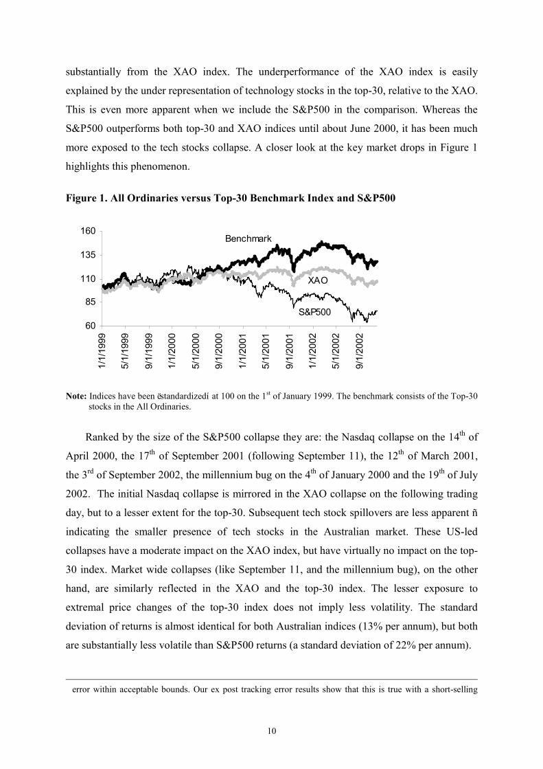
Figure 1 indicates that our top-30 benchmark tracks the XAO index quite closely for the

first year and a half of our sample. Mid 2000, however, the top-30 starts to diverge 6 The top-10 stocks already account for over 40% of the XAO. For comparison, the top-10 stocks in the S&P500 account for about 25%. This dominance of a few stocks should make it theoretically easy to keep the tracking

10

substantially from the XAO index. The underperformance of the XAO index is easily

explained by the under representation of technology stocks in the top-30, relative to the XAO.

This is even more apparent when we include the S&P500 in the comparison. Whereas the

S&P500 outperforms both top-30 and XAO indices until about June 2000, it has been much

more exposed to the tech stocks collapse. A closer look at the key market drops in Figure 1

highlights this phenomenon.

Figure 1. All Ordinaries versus Top-30 Benchmark Index and S&P500

60

85

110

135

160

1/1/1999

5/1/1999

9/1/1999

1/1/2000

5/1/2000

9/1/2000

1/1/2001

5/1/2001

9/1/2001

1/1/2002

5/1/2002

9/1/2002

S&P500

Benchmark

XAO

Note: Indices have been ëstandardizedí at 100 on the 1st of January 1999. The benchmark consists of the Top-30

stocks in the All Ordinaries.

Ranked by the size of the S&P500 collapse they are: the Nasdaq collapse on the 14th of

April 2000, the 17th of September 2001 (following September 11), the 12th of March 2001,

the 3rd of September 2002, the millennium bug on the 4th of January 2000 and the 19th of July

2002. The initial Nasdaq collapse is mirrored in the XAO collapse on the following trading

day, but to a lesser extent for the top-30. Subsequent tech stock spillovers are less apparent ñ

indicating the smaller presence of tech stocks in the Australian market. These US-led

collapses have a moderate impact on the XAO index, but have virtually no impact on the top-

30 index. Market wide collapses (like September 11, and the millennium bug), on the other

hand, are similarly reflected in the XAO and the top-30 index. The lesser exposure to

extremal price changes of the top-30 index does not imply less volatility. The standard

deviation of returns is almost identical for both Australian indices (13% per annum), but both

are substantially less volatile than S&P500 returns (a standard deviation of 22% per annum).

error within acceptable bounds. Our ex post tracking error results show that this is true with a short-selling

11

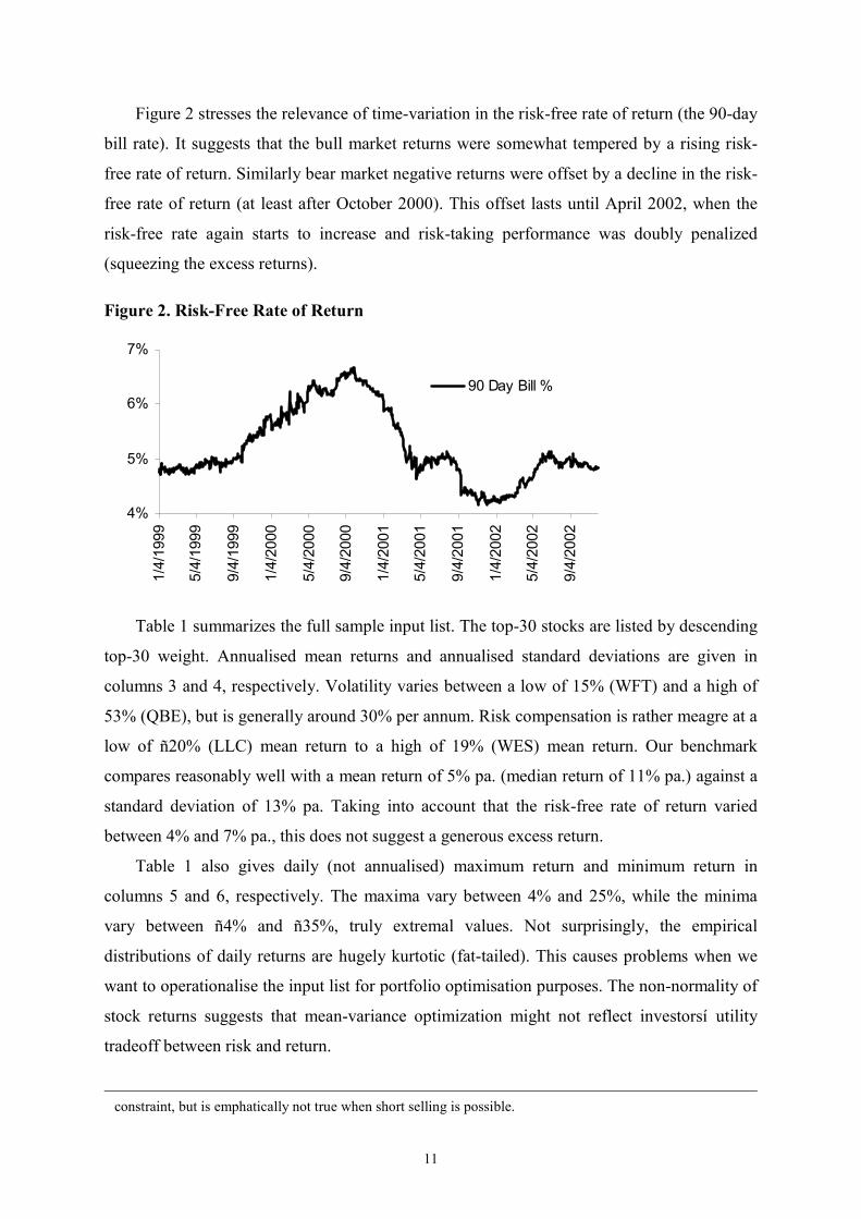
Figure 2 stresses the relevance of time-variation in the risk-free rate of return (the 90-day

bill rate). It suggests that the bull market returns were somewhat tempered by a rising risk-

free rate of return. Similarly bear market negative returns were offset by a decline in the risk-

free rate of return (at least after October 2000). This offset lasts until April 2002, when the

risk-free rate again starts to increase and risk-taking performance was doubly penalized

(squeezing the excess returns). Figure 2. Risk-Free Rate of Return

4%

5%

6%

7%

1/4/1999

5/4/1999

9/4/1999

1/4/2000

5/4/2000

9/4/2000

1/4/2001

5/4/2001

9/4/2001

1/4/2002

5/4/2002

9/4/2002

90 Day Bill %

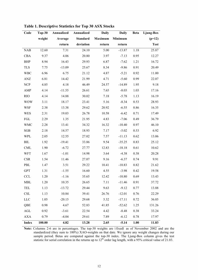
Table 1 summarizes the full sample input list. The top-30 stocks are listed by descending

top-30 weight. Annualised mean returns and annualised standard deviations are given in

columns 3 and 4, respectively. Volatility varies between a low of 15% (WFT) and a high of

53% (QBE), but is generally around 30% per annum. Risk compensation is rather meagre at a

low of ñ20% (LLC) mean return to a high of 19% (WES) mean return. Our benchmark

compares reasonably well with a mean return of 5% pa. (median return of 11% pa.) against a

standard deviation of 13% pa. Taking into account that the risk-free rate of return varied

between 4% and 7% pa., this does not suggest a generous excess return.

Table 1 also gives daily (not annualised) maximum return and minimum return in

columns 5 and 6, respectively. The maxima vary between 4% and 25%, while the minima

vary between ñ4% and ñ35%, truly extremal values. Not surprisingly, the empirical

distributions of daily returns are hugely kurtotic (fat-tailed). This causes problems when we

want to operationalise the input list for portfolio optimisation purposes. The non-normality of

stock returns suggests that mean-variance optimization might not reflect investorsí utility

tradeoff between risk and return.

constraint, but is emphatically not true when short selling is possible.

12

Table 1. Descriptive Statistics for Top 30 ASX Stocks Code Top-30

weight

Annualized

Average

return

Annualized

Standard

deviation

Daily

Maximum

return

Daily

Minimum

return

Beta Ljung-Box

(p=12)

Test

NAB 12.60 7.31 24.10 5.00 -13.87 1.18 25.87

CBA 9.37 4.06 20.80 3.97 -7.13 0.95 12.27

BHP 8.94 16.43 29.93 6.87 -7.62 1.21 16.72

TLS 7.75 -13.09 25.67 8.34 -9.86 0.91 20.49

WBC 6.96 6.75 21.12 4.87 -5.21 0.92 11.00

ANZ 6.81 14.42 21.99 4.71 -5.60 0.99 22.07

NCP 4.85 4.18 46.49 24.57 -14.89 1.95 9.18

AMP 4.14 -11.55 26.61 7.65 -8.03 1.03 17.16

RIO 4.14 14.88 30.02 7.18 -5.78 1.13 16.19

WOW 3.11 18.17 23.41 5.16 -8.34 0.53 28.93

WSF 2.38 13.38 29.62 20.92 -6.55 0.86 16.35

WES 2.31 19.03 26.78 10.58 -6.42 0.71 17.49

FGL 2.29 1.35 21.95 4.83 -7.06 0.49 36.79

WMC 2.28 13.41 34.32 16.32 -10.40 0.97 46.10

SGB 2.18 14.57 18.93 7.17 -5.02 0.53 6.92

WPL 2.05 12.55 27.02 7.57 -11.13 0.62 13.06

BIL 1.92 -19.41 33.86 9.54 -35.25 0.83 25.12

CML 1.90 -6.72 27.77 12.83 -18.18 0.61 10.62

WFT 1.67 -1.01 14.98 3.64 -4.38 0.38 20.28

CSR 1.54 11.46 27.07 9.16 -6.37 0.74 9.91

PBL 1.47 3.51 29.22 10.41 -10.83 0.82 21.62

GPT 1.31 -1.55 16.60 4.55 -3.98 0.42 19.58

CCL 1.20 -1.16 35.65 12.42 -10.80 0.69 13.43

MBL 1.20 10.35 26.65 7.11 -11.46 0.91 37.72

TEL 1.13 -13.72 29.44 9.63 -9.12 0.77 13.88

CSL 1.13 10.84 39.41 26.76 -12.01 0.76 22.29

LLC 1.05 -20.15 29.68 5.32 -17.11 0.72 36.05

QBE 0.98 4.67 52.83 41.85 -52.62 1.25 131.26

AGL 0.92 -3.61 22.54 4.42 -8.48 0.38 33.24

AXA 0.79 -4.04 29.61 7.89 -6.12 0.78 17.97

Index 100.00 4.82 13.28 2.65 -5.14 1.00 11.83

Note: Columns 2-6 are in percentages. The top-30 weights are ì fixedî as of November 2002 and are the standardized (they sum to 100%) XAO-weights on that date. We ignore any weight changes during our sample period. Betas are computed against the top-30 index. The Ljung-Box column gives the test statistic for serial correlation in the returns up to 12th order lag length, with a 95% critical value of 21.03.

13

Campbell et al. (2001) illustrate an alternative optimisation procedure that better captures

the kurtotic (and perhaps skewed) nature of stock returns. As a matter for future research, we

could incorporate an equivalent tracking error constraint in their optimisation procedure. As

long as the empirical distributions are symmetric, we expect very little difference in terms of

active weight selection.

Unlike stock analysts, we do not have the fundamentals (growth forecasts, accounting

information, etc.) to value and then rank stocks by forecast return to generate buy/sell signals.

Our information set is restricted to historical returns. For simplicity, consider the following

example where our forecast return is a simple average of the past 5 trading daysí returns. If

we happen to encounter a single extremal return in our information sample (say, 10.58%) and

four zero returns, we generate an annualised forecast return of 535%. Clearly, the extremal

return is non-representative for forecast purposes. Even for longer information samples (say a

month, or 20 trading days) this inflation of annualised forecast returns based on extremal

observations remains a problem. It reflects the fact that daily stock return distributions are not

normally distributed, but are better characterized by some fat-tailed distribution (like, e.g., a

Student-t). Unlike the normal distribution, a Student-t is not ì closed under addition,î i.e., its

properties (e.g., the variance) cannot be simply scaled to derive equivalents at a different

sampling frequency (say from daily to annualised).

This problem highlights the difficulties that one encounters when optimising portfolios

of individual stocks based on simplistic input list rules. It might explain why the academic

literature prefers to build efficient portfolios from portfolios of individual stocks7. ëIndexingí

clearly normalizes the empirical distributions (just consider the descriptive statistics for the

top-30 index), which makes these portfolios much more suitable for portfolio optimisation

purposes. This may be feasible for academic purposes, but it will not typically be a

satisfactory solution for practical purposes. To somehow moderate the impact of extremal

returns on our input list, we therefore choose to forecast returns based on a smoothed beta

model as explained in the previous section.

Of course, the validity of using past average returns to forecast future returns (either as a

simple average or as a market expectation) depends crucially on the stationarity of stock

returns. The Ljung-Box portmanteau statistic (autocorrelation up to lag length 12) in column

8, Table 1, indicates that quite a few series display significant autocorrelation (95% critical

7 The authors are well aware of more important reasons (like the errors-in-variables correction) for this choice.

14

value 212χ = 21.03). As suggested by Lawton-Browne (2001), this may lead to a downward

bias in ex ante tracking error. We investigate this below.

4. Empirical Results

To start our analysis, we first compute our input list. To update the vector of forecast returns,

E, we use a simplified version of the BARRA beta pricing model encapsulated in equations

(1) and (2). There is no real precedent for this procedure, and it obviously lends itself for

future improvement. We choose φ=0.34 for our application, but also investigate the

sensitivity of our results for different values of φ. This procedure generates fairly smoothly

evolving forecast returns.

To update the forecast variance-covariance matrix, we use the RiskMetricsTM EWMA

methodology. It is simple to understand, straightforward to implement, and generates

GARCH-like variance processes. To illustrate this point, consider the GARCH(1,1) output in

Figure 3 for NAB. The GARCH(1,1) parameters were estimated at α1=0.17, α2=0.74, while

the average decay factor in the EWMA was estimated to be λ=0.91 (with an effective

estimation sample length of 40 days). The EWMA process is somewhat smoother, but there

seems little to separate the two processes ñ a similar point is made in RiskMetricsô (1995).

Figure 3. NAB Conditional Volatility ñ GARCH(1,1) versus EWMA

0

0.25

0.5

0.75

1/4/1999

5/4/1999

9/4/1999

1/4/2000

5/4/2000

9/4/2000

1/4/2001

5/4/2001

9/4/2001

1/4/2002

5/4/2002

9/4/2002

Note: Annualized standard deviations for NAB are based on fitting a GARCH(1,1) model:

21,2

21,10

2−− σα+α+α=σ titiit R , respectively an EWMA model: ( )∑

∞

=−λλ−=σ

0

2,

2 1j

jtij

it R .

Whereas it is relatively straightforward to estimate a univariate GARCH(1,1) process

like the one above, the computational burden becomes excessive for a multivariate GARCH

process involving 30 stocks. Scowcroft and Sefton (2001) investigate the performance of a

EWMA

GARCH(1,1)

15

number of time-varying risk matrix specifications ñ including the EWMA and GARCH

models ñ and find that the tracking error predictions agreed reasonably well.

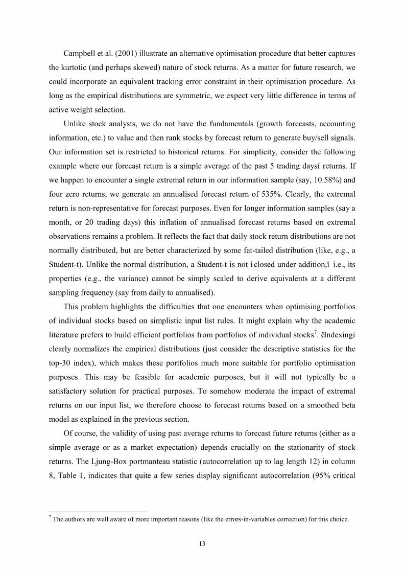
Figure 4 gives some insight in the dynamically updated input list for three stock

components in the top-30 benchmark: NAB (the largest weight, 12.6% and a full-sample

unconditional beta of 1.18), NCP (the highest full-sample unconditional beta, 1.95) and AGL

(the lowest full-sample unconditional beta, 0.38). Figure 4 shows the time variation in their

betas, according to equation (1).

Figure 4. Time Variation in Betas

0

0.5

1

1.5

2

2.5

3/3/1999

6/3/1999

9/3/1999

12/3/1999

3/3/2000

6/3/2000

9/3/2000

12/3/2000

3/3/2001

6/3/2001

9/3/2001

12/3/2001

3/3/2002

6/3/2002

9/3/2002

Note: Unconditional betas are respectively 1.18 (NAB), 1.95 (NCP), and 0.38 (AGL); Betas are measured

against the top-30 benchmark index.

NAB has the more stable beta, whereas NCP and AGL (the stocks with more extreme ñ high

and low ñ betas) have much more volatile intertemporal betas. This has obvious

repercussions for the forecast returns according to equation (2), where the more volatile beta

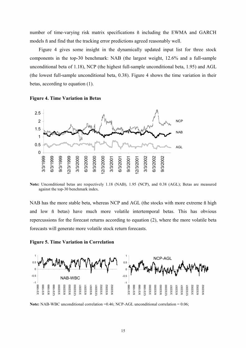
forecasts will generate more volatile stock return forecasts. Figure 5. Time Variation in Correlation

-1

-0.5

0

0.5

1

3/3/1999

6/3/1999

9/3/1999

12/3/1999

3/3/2000

6/3/2000

9/3/2000

12/3/2000

3/3/2001

6/3/2001

9/3/2001

12/3/2001

3/3/2002

6/3/2002

9/3/2002

-1

-0.5

0

0.5

1

3/3/1999

6/3/1999

9/3/1999

12/3/1999

3/3/2000

6/3/2000

9/3/2000

12/3/2000

3/3/2001

6/3/2001

9/3/2001

12/3/2001

3/3/2002

6/3/2002

9/3/2002

Note: NAB-WBC unconditional correlation =0.46; NCP-AGL unconditional correlation = 0.06;

AGL

NCP

NAB

NAB-WBC

NCP-AGL

16

Figure 5 illustrates the time-varying intra-sector correlation between NAB and WBC,

two banking stocks in our universe; respectively between NCP and AGL for an inter-sector

illustration. Intra- and inter-sector time-varying correlation are equally volatile, but obviously

have a different mean. The intra-sector correlation displays switching behaviour with periods

of high correlation alternating with periods of low correlation and not much in between. The

inter-sector correlation does not share this feature.

Having completed the input list, we can proceed to compute the efficient frontier solving

(4) with λ=0.91. Then we solve (6í) to obtain the active tracking error frontier with a tracking

error target of 5%. Our top-30 benchmark is found to be seriously inefficient (throughout our

sample period with a few exceptions when it is close to the global efficient frontier) which

suggests active investment opportunities. Or, in ex ante Information Ratio terms, they offer a

positive IR for active portfolio managers. To illustrate this, consider the following two

representative optimization periods. Figures 6a and 6b are representative for a bull market

episode, respectively a bear market episode. As expected in a bull (bear) market the active

investment opportunity set ñ the ellipse ñ is upward (downward) sloping. The benchmark (the

square symbol) typically has lower risk than the individual stocks (the diamond symbols) but

of course, only average expected returns.

Figure 6. Bulls and Bears

-0.2

0

0.2

0.4

0.6

0.8

1

0 0.1 0.2 0.3 0.4 0.5

-0.5

-0.4

-0.3

-0.2

-0.1

0

0.1

0.2

0.3

0.4

0.5

0 0.1 0.2 0.3 0.4

Efficient Frontier Constrained Active Portfolio

Constant Tracking Error Frontier Unconstrained Active Portfolio

No Short Selling Efficient Frontier Benchmark Portfolio

The location of the active portfolios chosen in the previous period optimisation is also

indicated in both graphs. Without rebalancing, the unconstrained active portfolio (circle

symbol outside ellipse) needs no longer be on the updated ellipse. As it turns out, the

constrained active portfolio (circle symbol inside ellipse) is always inside the updated ellipse,

17

but the unconstrained active portfolio is almost without exception outside the updated

tracking error frontier. That does not necessarily imply a violation of the tracking error

constraint over that period, but does imply an ex ante tracking error violation for the

subsequent period.

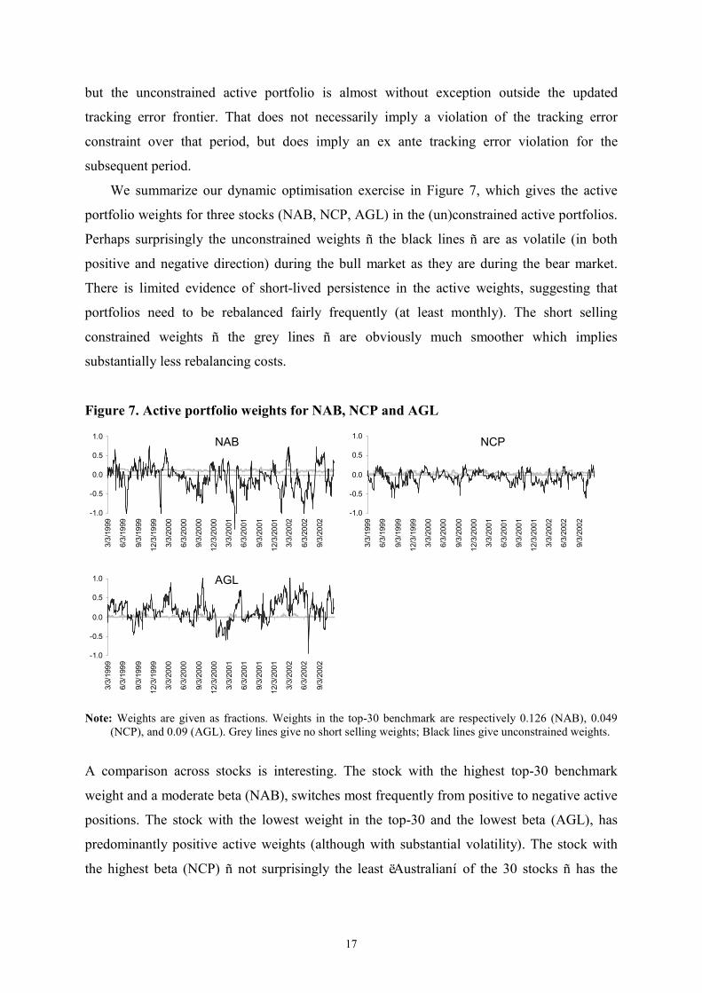
We summarize our dynamic optimisation exercise in Figure 7, which gives the active

portfolio weights for three stocks (NAB, NCP, AGL) in the (un)constrained active portfolios.

Perhaps surprisingly the unconstrained weights ñ the black lines ñ are as volatile (in both

positive and negative direction) during the bull market as they are during the bear market.

There is limited evidence of short-lived persistence in the active weights, suggesting that

portfolios need to be rebalanced fairly frequently (at least monthly). The short selling

constrained weights ñ the grey lines ñ are obviously much smoother which implies

substantially less rebalancing costs.

Figure 7. Active portfolio weights for NAB, NCP and AGL

-1.0

-0.5

0.0

0.5

1.0

3/3/1999

6/3/1999

9/3/1999

12/3/1999

3/3/2000

6/3/2000

9/3/2000

12/3/2000

3/3/2001

6/3/2001

9/3/2001

12/3/2001

3/3/2002

6/3/2002

9/3/2002

-1.0

-0.5

0.0

0.5

1.0

3/3/1999

6/3/1999

9/3/1999

12/3/1999

3/3/2000

6/3/2000

9/3/2000

12/3/2000

3/3/2001

6/3/2001

9/3/2001

12/3/2001

3/3/2002

6/3/2002

9/3/2002

-1.0

-0.5

0.0

0.5

1.0

3/3/1999

6/3/1999

9/3/1999

12/3/1999

3/3/2000

6/3/2000

9/3/2000

12/3/2000

3/3/2001

6/3/2001

9/3/2001

12/3/2001

3/3/2002

6/3/2002

9/3/2002

Note: Weights are given as fractions. Weights in the top-30 benchmark are respectively 0.126 (NAB), 0.049

(NCP), and 0.09 (AGL). Grey lines give no short selling weights; Black lines give unconstrained weights.

A comparison across stocks is interesting. The stock with the highest top-30 benchmark

weight and a moderate beta (NAB), switches most frequently from positive to negative active

positions. The stock with the lowest weight in the top-30 and the lowest beta (AGL), has

predominantly positive active weights (although with substantial volatility). The stock with

the highest beta (NCP) ñ not surprisingly the least ëAustralianí of the 30 stocks ñ has the

NAB NCP

AGL

18

most stable active weights (although they switch frequently from positive to negative and

vice versa without much persistence).

Since we rebalance every time period, our ex ante tracking error is always exactly equal

to the target. This is clearly not the case ex post. The problem now is how to measure the ex

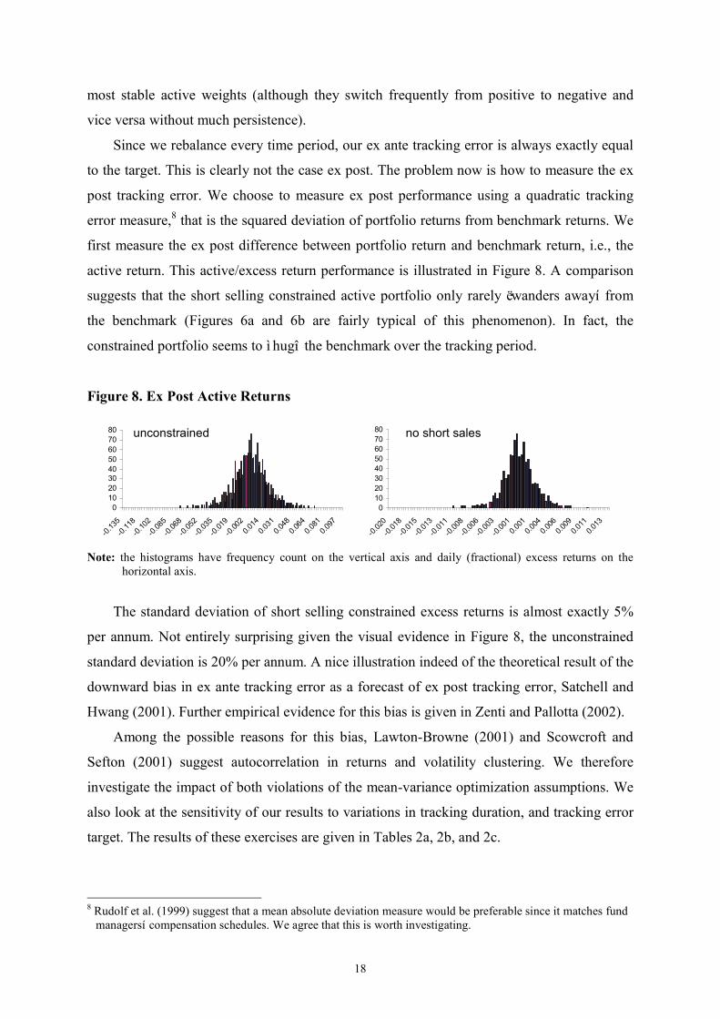
post tracking error. We choose to measure ex post performance using a quadratic tracking

error measure,8 that is the squared deviation of portfolio returns from benchmark returns. We

first measure the ex post difference between portfolio return and benchmark return, i.e., the

active return. This active/excess return performance is illustrated in Figure 8. A comparison

suggests that the short selling constrained active portfolio only rarely ëwanders awayí from

the benchmark (Figures 6a and 6b are fairly typical of this phenomenon). In fact, the

constrained portfolio seems to ì hugî the benchmark over the tracking period.

Figure 8. Ex Post Active Returns

01020304050607080

-0.135-0.118-0.102-0.085-0.068-0.052-0.035-0.019-0.0020.0140.0310.0480.0640.0810.097

01020304050607080

-0.020-0.018-0.015-0.013-0.011-0.008-0.006-0.003-0.0010.0010.0040.0060.0090.0110.013

Note: the histograms have frequency count on the vertical axis and daily (fractional) excess returns on the

horizontal axis.

The standard deviation of short selling constrained excess returns is almost exactly 5%

per annum. Not entirely surprising given the visual evidence in Figure 8, the unconstrained

standard deviation is 20% per annum. A nice illustration indeed of the theoretical result of the

downward bias in ex ante tracking error as a forecast of ex post tracking error, Satchell and

Hwang (2001). Further empirical evidence for this bias is given in Zenti and Pallotta (2002).

Among the possible reasons for this bias, Lawton-Browne (2001) and Scowcroft and

Sefton (2001) suggest autocorrelation in returns and volatility clustering. We therefore

investigate the impact of both violations of the mean-variance optimization assumptions. We

also look at the sensitivity of our results to variations in tracking duration, and tracking error

target. The results of these exercises are given in Tables 2a, 2b, and 2c.

8 Rudolf et al. (1999) suggest that a mean absolute deviation measure would be preferable since it matches fund managersí compensation schedules. We agree that this is worth investigating.

unconstrained no short sales

19

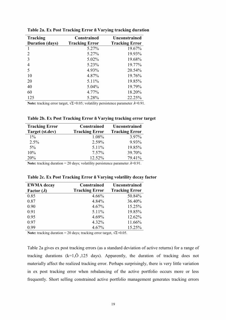
Table 2a. Ex Post Tracking Error ñ Varying tracking duration

Tracking Duration (days)

Constrained Tracking Error

Unconstrained Tracking Error

1 5.27% 19.67%2 5.27% 19.93%3 5.02% 19.68%4 5.23% 19.77%5 4.93% 20.54%10 4.87% 19.76%20 5.11% 19.85%40 5.04% 19.79%60 4.77% 18.20%125 5.28% 22.25%Note: tracking error target, √Σ=0.05; volatility persistence parameter λ=0.91.

Table 2b. Ex Post Tracking Error ñ Varying tracking error target

Tracking Error Target (st.dev)

Constrained Tracking Error

Unconstrained Tracking Error

1% 1.08% 3.97% 2.5% 2.59% 9.93% 5% 5.11% 19.85%10% 7.57% 39.70%20% 12.52% 79.41%Note: tracking duration = 20 days; volatility persistence parameter λ=0.91.

Table 2c. Ex Post Tracking Error ñ Varying volatility decay factor

EWMA decay Factor (λ)

Constrained Tracking Error

Unconstrained Tracking Error

0.85 4.66% 50.84%0.87 4.84% 36.40%0.90 4.67% 15.25%0.91 5.11% 19.85%0.95 4.69% 12.62%0.97 4.32% 11.66%0.99 4.67% 15.25%Note: tracking duration = 20 days; tracking error target, √Σ=0.05.

Table 2a gives ex post tracking errors (as a standard deviation of active returns) for a range of

tracking durations (k=1,Ö ,125 days). Apparently, the duration of tracking does not

materially affect the realized tracking error. Perhaps surprisingly, there is very little variation

in ex post tracking error when rebalancing of the active portfolio occurs more or less

frequently. Short selling constrained active portfolio management generates tracking errors

20

that stay within the target tracking error. Unconstrained active portfolio management

generates tracking errors well in excess of the target.

Table 2b gives ex post tracking error for a range of tracking error targets (√Σ=1%,

Ö ,20%). We observe that the ex post short selling constrained tracking error marginally

exceeds (is substantially less than) the ex ante tracking error for targets below (above) 5% per

annum. Ex post unconstrained tracking error, however, generally exceeds the ex ante tracking

error at an increasing rate with increasing target tracking error.

Table 2c suggests the source of the bias in ex ante tracking error expectations. It gives ex

post tracking errors for a range of EWMA decay factors (λ=0.85, Ö ,0.99). For this

(admittedly limited in scope) experiment, we find that at λ=0.97, the bias is minimized. We

suspect that individual optimisation of the λ parameter for each and every element in the

variance-covariance matrix would allow an even better outcome.

We also experimented with the serial correlation in stock returns by varying the

smoothing parameter φ in (1). This did not affect the bias in ex ante tracking error. It does, of

course, affect the location of the excess return distribution, but not the scale!

Bringing the two results (time-variation in weights and ex post performance) together

suggests that the typical short selling constraint acts as a safeguard on ex post tracking error

while simultaneously reducing the cost of rebalancing. A short selling constraint effectively

turns active portfolio management into something very close to passive portfolio

management. So why do we not observe the matching reduction in active returns? Simply

because we made no real attempt to actively forecast stock returns. In fact, we have taken a

rather ëpassiveí approach when generating the input list9. We can imagine that stock analysts

(or sophisticated econometriciansí models for that matter) are able to manipulate these active

performance distributions to their benefit and hence change the location of the active return

distributions in Figure 8 accordingly.

5. Conclusions

Although straightforward in content, proper implementation of portfolio optimization theory

can be notoriously complicated. Choices have to be made with regard to the input list,

constraints, estimation procedure, and implied actions. This paper gives a flavour of some of

the many issues that have to be dealt with by portfolio managers. The main advantage of our

9 We use a mechanistic rule ñ as in equation (2) ñ to generate expected returns. Our choice of the smoothing parameter φ is not based on proper model selection criteria, since this was not the main focus of our paper.

21

procedure is its transparent nature which considerably facilitates communication with an ever

more sophisticated clientele.

Jorionís (2002) main contribution is the visualization of the ì active investment

opportunity space.î We illustrate that the introduction of a short selling constraint eliminates

most of this opportunity set ñ partly driven by persistent bear market conditions during our

sample period. However, as an investment advice tool, successive introduction of investment

constraints clearly identifies the location of (and the reduction in) the relevant investment

opportunity set. The methodology also highlights the tradeoff between risk penalty and

excess return gain when violating the investment constraints. From this perspective, Jorionís

methodology is an invaluable contribution to the practical investment literature.

We find (as do many others, see e.g., Plaxco and Arnott, 2002) that frequent rebalancing

is an absolute necessity to keep some control over total risk (though not necessarily tracking

error risk) when actively managing portfolios. Larsen and Resnick (2001) consider a range of

optimization and holding periods, but do not consider transaction cost constraints. Clearly,

the costs of rebalancing have to be offset against the gains in risk control, but it seems to us

that certain (threshold) levels of risk will simply be unacceptable. The issue, of course, is how

to optimally rebalance so as to minimize the control costs.

Not surprisingly, we also find that ex ante tracking error expectations do not match ex

post realizations, see also Rohweder (1998). Satchell and Hwang (2001) show that we can

reasonably expect a worse ex post tracking error outcome due to the stochastic nature of

portfolio weights. They report that this upward bias is not restricted to active portfolios, but

can also be found in passive portfolios where the weights are not stochastic (due to

rebalancing). A similar upward bias in ex post tracking error (but due to a different source) is

caused by the apparent serial correlation, not just in the underlying stock returns, but also in

the excess returns and squared excess returns. Frino and Gallagher (2001), e.g., find evidence

of seasonality in tracking error (partly driven by seasonality in dividend payments on the

benchmark). Pope and Yadavís (1994) results indicate that this will lead to a biased ex ante

estimate of tracking error.

Where to from here? There is plenty of scope to improve the selection of optimal

observation period and forecast period duration. Ultimately, this is an empirical matter. We

hinted at the possibility (and Table 2b underlines its importance) to individualize the

stochastic processes for every element of the variance-covariance matrix. A trade-off will

then have to be made between the improvement in goodness-of-fit and the increased

22

computational burden of such an exercise. Despite this, we argue that there is no urgent need

to resort to computationally burdensome multivariate GARCH specifications.

Another constraint worth investigating is a cap on the number of stocks in the managed

portfolio or the minimum number of stocks in an active portfolio. Jansen and van Dijk (2002)

illustrate the small portfolio constraint for a passive tracking portfolio. Ammann and

Zimmermann (2001) investigate admissible active weight ranges, which would guarantee a

limit on individual stock weights. Alternatively, we could investigate a cap on the number of

stocks in which the portfolio manager takes active positions, while taking neutral positions in

the remaining benchmark component stocks. Yet another approach could be a factor-

neutrality constraint as in Clarke et al. (2002), which would fit typical style-type portfolio

constraints. It is quite possible that some of these constraints are internally conflicting. The

long-only constraint, e.g., tends to favour small capitalization active stock weights, which

would obviously clash with a large capitalization style constraint.

Another issue is the composition of the benchmark. Fund managers can frequently

choose their benchmarks (within reasonable boundaries, i.e., among a peer group). Small cap

fund managers would typically choose a representative small cap benchmark, like the ASX

Small Ords. As shown in Larsen and Resnick (1998), the market capitalization of component

stocks in the benchmark index has a non-trivial impact on the tracking performance of

enhanced benchmark portfolios. Though their analysis quantifies the impact, they are not

explicit on the source. It could be a liquidity constraint, or perhaps the (related) excessive

non-normality of the returns of these stocks.

A few papers have recently focused on tracking error measurement that better reflects the

incentive structure of the portfolio manager, see e.g., Kritzman (1987) and Rudolf et al.

(1999). Roll (1992) suggests that diversification of an investorís portfolio across managers

reduces the impact of excessively risky active portfolios. Jorion (2002) shows that this is not

a satisfactory solution and instead favours additional constraints on total risk to better control

for the free option provided to portfolio managers who are only constrained by active risk (or

tracking error). A closer look at investorsí utility functions and better integration of these

utility functions with constrained portfolio optimizations seems a worthwhile extension of

this paper.

Perhaps most importantly, there needs to be more research towards proper integration of

return and risk forecasts. Though it seems obvious that stock analysts do make risk

assessments when computing forecast returns, it is much less obvious to extract and combine

these risk assessments into a justifiable risk measure.

23

References

Ammann, M. and H. Zimmermann, 2001. Tracking error and tactical asset allocation. Financial Analysts Journal 57, 32-43.

Blair, B., 2002. Conditional asset allocation using prediction intervals to produce allocation decisions. Journal of Asset Management 2, 325-335.

Blasco, N., and R. Santamaria, 2001. Highest-density forecast regions: an essay in the Spanish stock market. Journal of Asset Management 2, 274-283.

Campbell, R., Huisman, R. and K. Koedijk, 2001. Optimal portfolio selection in a Value-at-Risk framework. Journal of Banking and Finance 25, 1789-1804.

Chan, L.K.C., and J. Lakonishok, 1993. Are the reports of betaís death premature? Journal of Portfolio Management 19, 51-62.

Chan, L.K.C., J. Karceski, and J. Lakonishok, 1999. On portfolio optimization: Forecasting covariances and choosing the risk model. Review of Financial Studies 12, 937-974.

Clarke, R., H. de Silva, and S. Thorley, 2002. Portfolio constraints and the fundamental law of active management. Financial Analysts Journal 58, 48-66.

Elton, E.J., M.J. Gruber, S.J. Brown, and W.N. Goetzmann, 2003. Modern portfolio theory and investment analysis. John Wiley & Sons, New York.

Engle, R.F., 1982. Autoregressive conditional heteroskedasticity with estimates of the variance of U.K. inflation. Econometrica 50, 987-1008.

Frino, A., and D.R. Gallagher, 2001. Tracking S&P 500 Index funds. Journal of Portfolio Management 28, 44-55.

Grinold, R.C., and R.N. Kahn, 1999. Active portfolio management. 2nd edition. McGraw-Hill: New York, NY.

Jansen, R., and R. van Dijk, 2002. Optimal benchmark tracking with small portfolios. Journal of Portfolio Management 29, 33-39.

Jorion, P., 2002, Portfolio optimization with constraints on tracking error. Financial Analysts Journal, forthcoming.

Kritzman, M., 1987. Incentive fees: Some problems and some solutions. Financial Analysts Journal 43, 21-26.

Larsen, G.A., and B.G. Resnick, 1998. Empirical insights on indexing. Journal of Portfolio Management 25, 27-34.

Larsen, G.A., and B.G. Resnick, 2001. Parameter estimation techniques, optimization frequency, and portfolio return enhancement. Journal of Portfolio Management 28, 27-34.

Lawton-Browne, C., 2001. An alternative calculation of tracking error. Journal of Asset Management 2, 223-234.

Plaxco, L.M., and R.D. Arnott, 2002. Rebalancing a global policy benchmark. Journal of Portfolio Management 29, 9-22.

Pope, P., and P.K. Yadav, 1994. Discovering the error in tracking error. Journal of Portfolio Management 21, 27-32.

RiskMetricsTM, 1995. Technical Document. 3rd Edition. Rohweder, H.C., 1998. Implementing stock selection ideas: Does tracking error optimization do any good? Journal of Portfolio Management 25, 49-59.

Roll, R., 1992. A mean/variance analysis of tracking error. Journal of Portfolio Management 18, 13-22.

Rosenberg, B., 1985. Prediction of common stock betas. Journal of Portfolio Management 11 (2), 5-14.

Rosenberg, B., and J. Guy, 1976. Beta and investment fundamentals. Financial Analysts Journal 32, 60-72.

Rudd, A., 1980. Optimal selection of passive portfolios. Financial Management 4, 57-66.

24

Rudd, A., and B. Rosenberg, 1980. The ëMarket Modelí in investment management. Journal of Finance 35, 597-606.

Rudolf, M., H-J. Wolter, and H. Zimmermann, 1999. A linear model for tracking error minimization. Journal of Banking and Finance 23, 85-103.

Satchell, S.E., and S. Hwang, 2001. Tracking error: Ex-ante versus ex-post measures. Journal of Asset Management 2, 241-246.

Scowcroft, A., and J. Sefton, 2001. Do tracking errors reliably estimate portfolio risk? Journal of Asset Management 2, 205-222.

Timmermann, A., and D. Blake, 2002. International asset allocation with time-varying investment opportunities. Forthcoming in Journal of Business.

Treynor, J., and F. Black, 1973. How to use security analysis to improve portfolio selection. Journal of Business 46, 66-86.

Zenti, R., and M. Pallotta, 2002. Are asset managers properly using tracking error estimates? Journal of Asset Management 3, 279-289.