Tracker 5.0 Help

Tracker is a free video analysis and modeling tool built on the Open Source Physics (OSP) Javaframework. Features include object tracking with position, velocity and acceleration overlays and graphs,special effect filters, multiple reference frames, calibration points, line profiles for analysis of spectra andinterference patterns, and dynamic particle models. It is designed to be used in introductory college physicslabs and lectures.

To start using Tracker, see getting started.

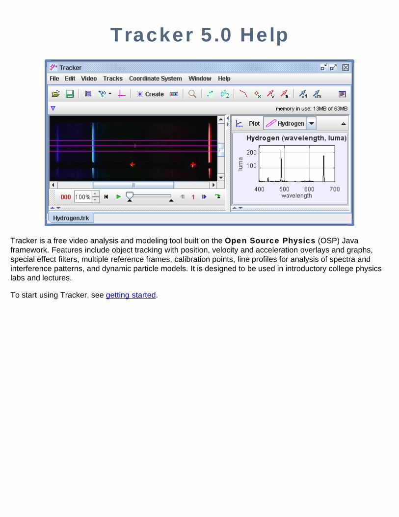
Getting StartedWhen you first open Tracker it appears as shown below. Here's how to start analyzing a video:

1. Open a video or tracker file.2. Identify the frames ("video clip") you wish to analyze.3. Calibrate the video scale.4. Set the reference frame origin and angle.5. Track objects of interest with the mouse.6. Plot and analyze the tracks.7. Save your work in a tracker file.8. Export track data to a spreadsheet.9. Print, save or copy/paste images for reports.

Note that the order of the buttons on the toolbar mirrors the steps used to analyze a video. For more information about Tracker'suser interface, including user customization, see user interface.

1. Open a video or tracker fileClick the Open button or File|Open File menu item and select a digital video (mov, avi, mp4, flv, wmv, etc.), tracker datafile (.trk), or zipped tracker file (.zip) to open. You can also open still and animated image files (.jpg, .gif, .png), numberedsequences of image files, and images pasted from the clipboard.

Play, scan or step through the video using the video player. For more information see videos.

Another option is to open the OSP Digital Library Browser by clicking the Open Library Browser button or choosingthe File|Open Library Browser menu item. The library browser enables you to browse and access collections of digitallibrary resources including videos and tracker files. For help using the OSP Digital Library Browser, choose its Help|LibraryBrowser Help menu item.

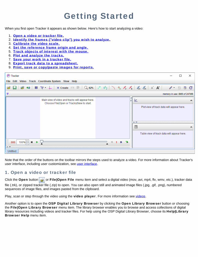
2. Identify the frames ("video clip") you wish to analyzeDisplay the clip settings by clicking the Clip Settings button on the toolbar.

In the clip settings dialog, set the Start frame and End frame to define the range you wish to analyze. You can drag theplayer's slider to scan through the video and quickly find the frames of interest. If the video contains too many frames to analyze(more than 20 or so can become tedious), increase the Step size to automatically skip frames.

You can also set these video clip properties directly on the video player. For more information see video clips.

3. Calibrate the scaleClick the Calibration button and select the calibration stick.

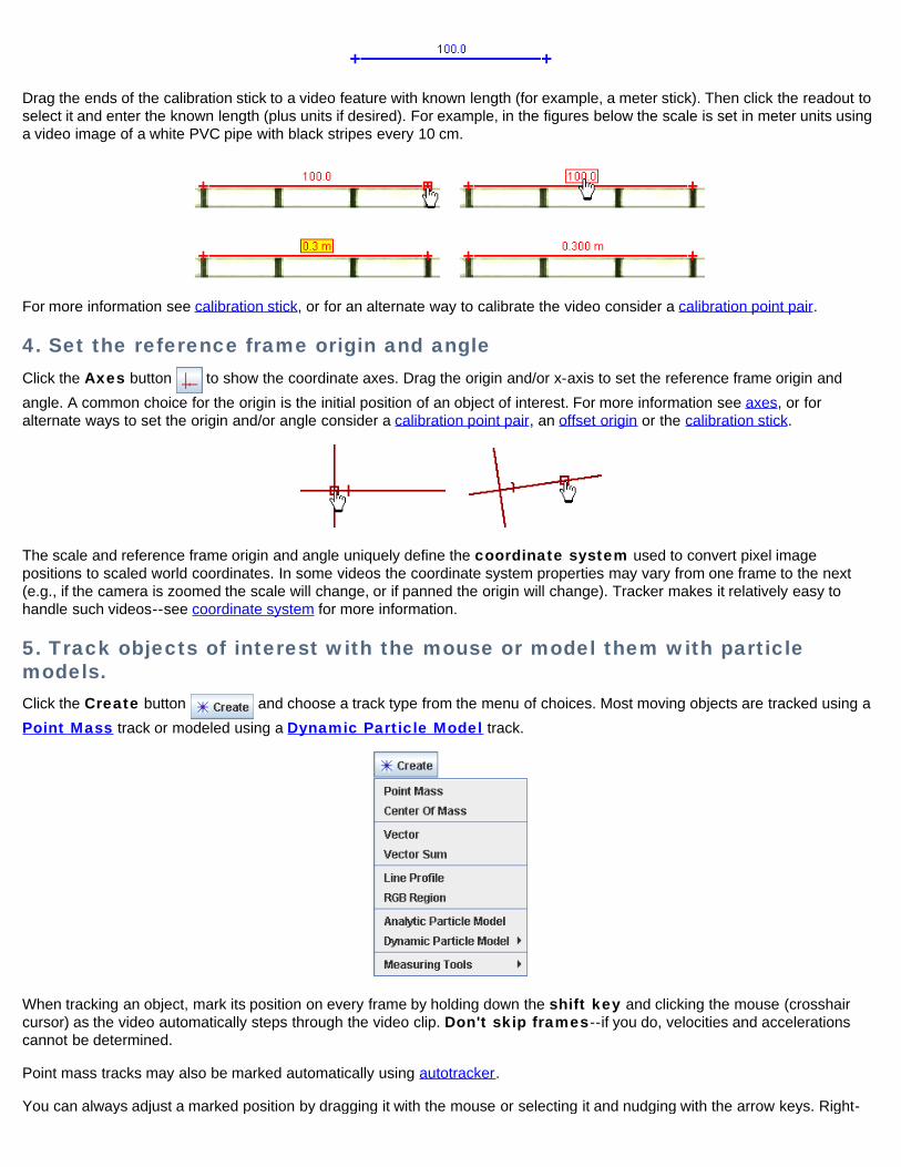
Drag the ends of the calibration stick to a video feature with known length (for example, a meter stick). Then click the readout toselect it and enter the known length (plus units if desired). For example, in the figures below the scale is set in meter units usinga video image of a white PVC pipe with black stripes every 10 cm.

For more information see calibration stick, or for an alternate way to calibrate the video consider a calibration point pair.

4. Set the reference frame origin and angleClick the Axes button to show the coordinate axes. Drag the origin and/or x-axis to set the reference frame origin andangle. A common choice for the origin is the initial position of an object of interest. For more information see axes, or foralternate ways to set the origin and/or angle consider a calibration point pair, an offset origin or the calibration stick.

The scale and reference frame origin and angle uniquely define the coordinate system used to convert pixel imagepositions to scaled world coordinates. In some videos the coordinate system properties may vary from one frame to the next(e.g., if the camera is zoomed the scale will change, or if panned the origin will change). Tracker makes it relatively easy tohandle such videos--see coordinate system for more information.

5. Track objects of interest with the mouse or model them with particlemodels.Click the Create button and choose a track type from the menu of choices. Most moving objects are tracked using aPoint Mass track or modeled using a Dynamic Particle Model track.

When tracking an object, mark its position on every frame by holding down the shift key and clicking the mouse (crosshaircursor) as the video automatically steps through the video clip. Don't skip frames--if you do, velocities and accelerationscannot be determined.

Point mass tracks may also be marked automatically using autotracker.

You can always adjust a marked position by dragging it with the mouse or selecting it and nudging with the arrow keys. Right-

click the video to zoom in for sub-pixel accuracy.

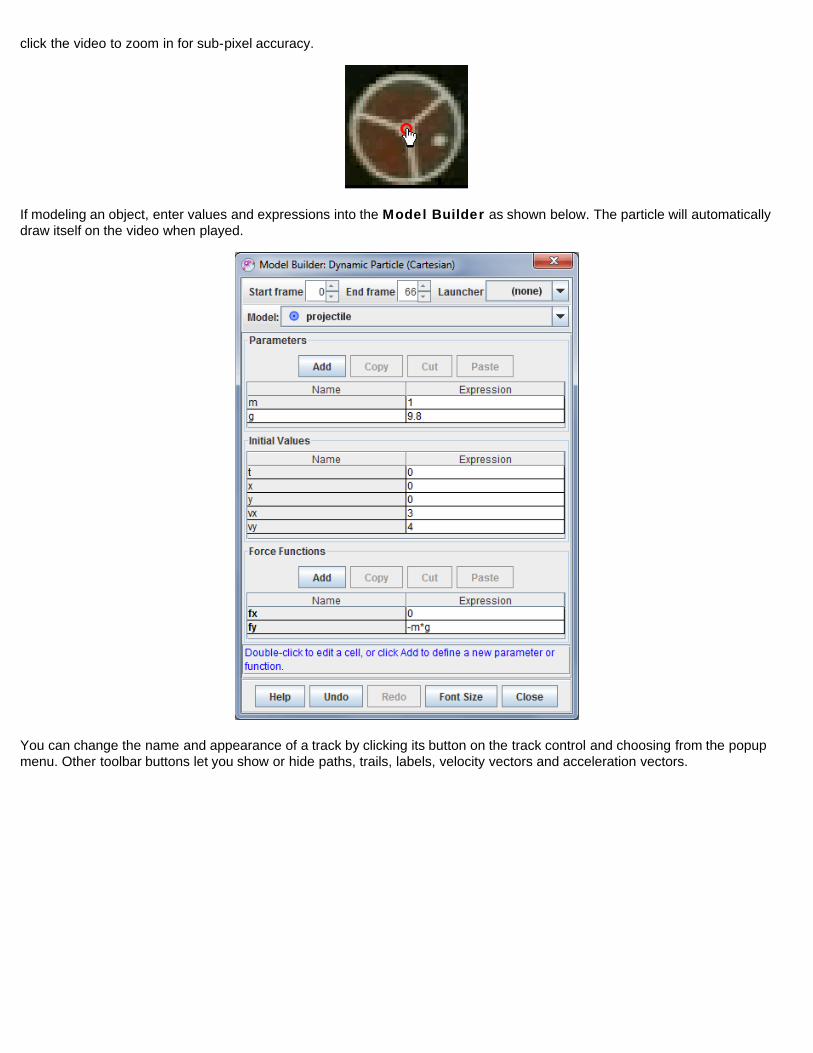
If modeling an object, enter values and expressions into the Model Builder as shown below. The particle will automaticallydraw itself on the video when played.

You can change the name and appearance of a track by clicking its button on the track control and choosing from the popupmenu. Other toolbar buttons let you show or hide paths, trails, labels, velocity vectors and acceleration vectors.

For more information on tracks and the track control, see tracks. For detailed information on a specific track type, see pointmass, center of mass, vector, vector sum, line profile, rgb region, particle model or two-body system.

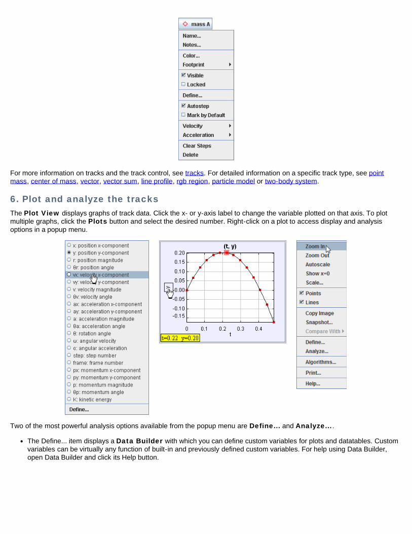
6. Plot and analyze the tracksThe Plot View displays graphs of track data. Click the x- or y-axis label to change the variable plotted on that axis. To plotmultiple graphs, click the Plots button and select the desired number. Right-click on a plot to access display and analysisoptions in a popup menu.

Two of the most powerful analysis options available from the popup menu are Define... and Analyze....

The Define... item displays a Data Builder with which you can define custom variables for plots and datatables. Customvariables can be virtually any function of built-in and previously defined custom variables. For help using Data Builder,open Data Builder and click its Help button.

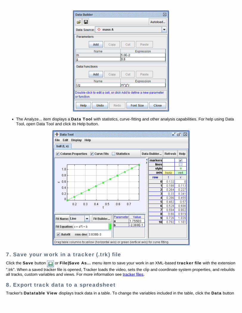
The Analyze... item displays a Data Tool with statistics, curve-fitting and other analysis capabilities. For help using DataTool, open Data Tool and click its Help button.

7. Save your work in a tracker (.trk) fileClick the Save button or File|Save As... menu item to save your work in an XML-based tracker file with the extension".trk". When a saved tracker file is opened, Tracker loads the video, sets the clip and coordinate system properties, and rebuildsall tracks, custom variables and views. For more information see tracker files.

8. Export track data to a spreadsheetTracker's Datatable View displays track data in a table. To change the variables included in the table, click the Data button

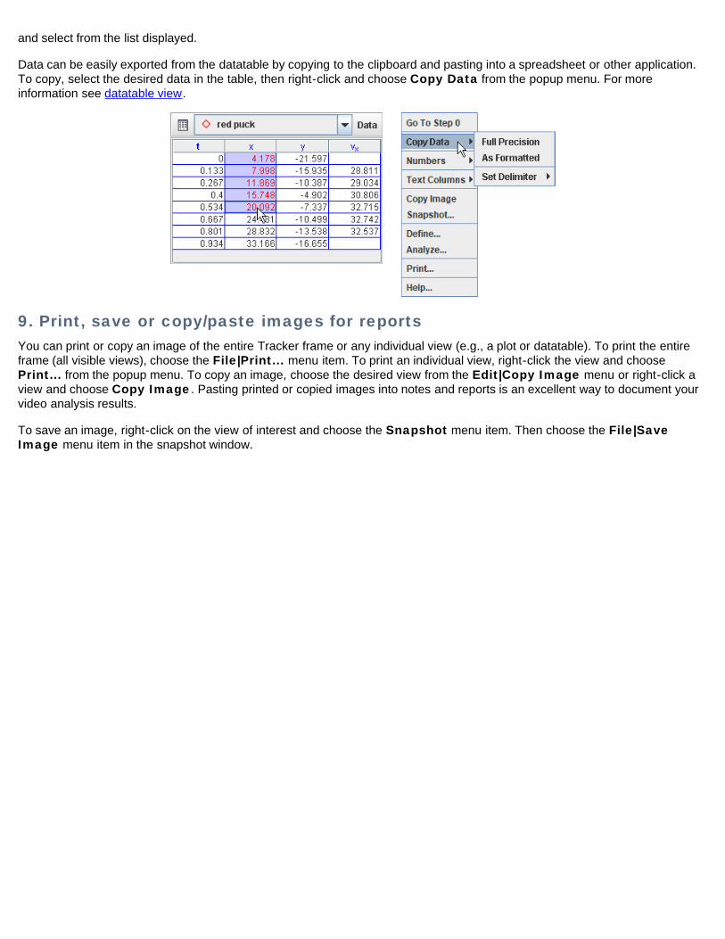
and select from the list displayed.

Data can be easily exported from the datatable by copying to the clipboard and pasting into a spreadsheet or other application.To copy, select the desired data in the table, then right-click and choose Copy Data from the popup menu. For moreinformation see datatable view.

9. Print, save or copy/paste images for reportsYou can print or copy an image of the entire Tracker frame or any individual view (e.g., a plot or datatable). To print the entireframe (all visible views), choose the File|Print... menu item. To print an individual view, right-click the view and choosePrint... from the popup menu. To copy an image, choose the desired view from the Edit|Copy Image menu or right-click aview and choose Copy Image. Pasting printed or copied images into notes and reports is an excellent way to document yourvideo analysis results.

To save an image, right-click on the view of interest and choose the Snapshot menu item. Then choose the File|SaveImage menu item in the snapshot window.

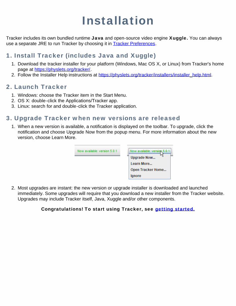
InstallationTracker includes its own bundled runtime Java and open-source video engine Xuggle. You can alwaysuse a separate JRE to run Tracker by choosing it in Tracker Preferences.

1. Install Tracker (includes Java and Xuggle)1. Download the tracker installer for your platform (Windows, Mac OS X, or Linux) from Tracker's home

page at https://physlets.org/tracker/.2. Follow the Installer Help instructions at https://physlets.org/tracker/installers/installer_help.html.

2. Launch Tracker1. Windows: choose the Tracker item in the Start Menu.2. OS X: double-click the Applications/Tracker app.3. Linux: search for and double-click the Tracker application.

3. Upgrade Tracker when new versions are released1. When a new version is available, a notification is displayed on the toolbar. To upgrade, click the

notification and choose Upgrade Now from the popup menu. For more information about the newversion, choose Learn More.

2. Most upgrades are instant: the new version or upgrade installer is downloaded and launchedimmediately. Some upgrades will require that you download a new installer from the Tracker website.Upgrades may include Tracker itself, Java, Xuggle and/or other components.

Congratulations! To start using Tracker, see getting started.

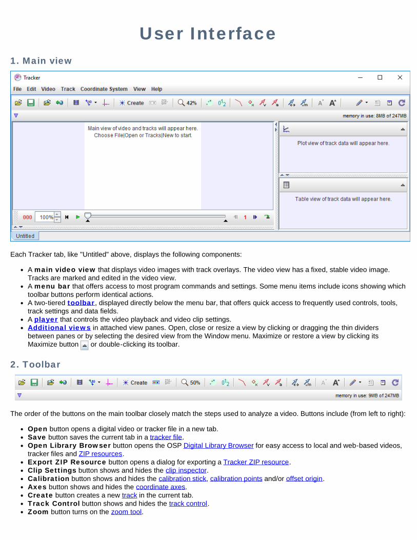
User Interface1. Main view

Each Tracker tab, like "Untitled" above, displays the following components:

A main video view that displays video images with track overlays. The video view has a fixed, stable video image.Tracks are marked and edited in the video view.A menu bar that offers access to most program commands and settings. Some menu items include icons showing whichtoolbar buttons perform identical actions.A two-tiered toolbar, displayed directly below the menu bar, that offers quick access to frequently used controls, tools,track settings and data fields.A player that controls the video playback and video clip settings.Additional views in attached view panes. Open, close or resize a view by clicking or dragging the thin dividersbetween panes or by selecting the desired view from the Window menu. Maximize or restore a view by clicking itsMaximize button or double-clicking its toolbar.

2. Toolbar

The order of the buttons on the main toolbar closely match the steps used to analyze a video. Buttons include (from left to right):

Open button opens a digital video or tracker file in a new tab.Save button saves the current tab in a tracker file.Open Library Browser button opens the OSP Digital Library Browser for easy access to local and web-based videos,tracker files and ZIP resources.Export ZIP Resource button opens a dialog for exporting a Tracker ZIP resource.Clip Settings button shows and hides the clip inspector.Calibration button shows and hides the calibration stick, calibration points and/or offset origin.Axes button shows and hides the coordinate axes.Create button creates a new track in the current tab.Track Control button shows and hides the track control.Zoom button turns on the zoom tool.

Trails button sets the length of all trails.Labels button shows and hides all labels.Path button shows and hides all paths.Positions button shows and hides all point mass positions.Velocities button shows and hides all point mass velocity vectors.Accelerations button shows and hides all point mass acceleration vectors.Stretch button stretches all vectors.Dynamics button multiplies all motion vectors by mass.Font Up and Down buttons control font and icon sizes.

Buttons near the right end of the toolbar control documentation tools and refreshes data:

Drawing button shows and hides the drawing control for annotating the video with line drawings and labels.Documents button displays supplemental HTML and/or PDF documents associated with a Tracker ZIP file.Notes button shows and hides the notes window for user descriptions of tracks and videos.Refresh button refreshes track data and views and turns auto-refresh on and off.

The lower tier of the toolbar is used mainly for selected track data and input fields, but also contains a memory managerbutton that manages and monitors Tracker's memory status. See memory management for more information.

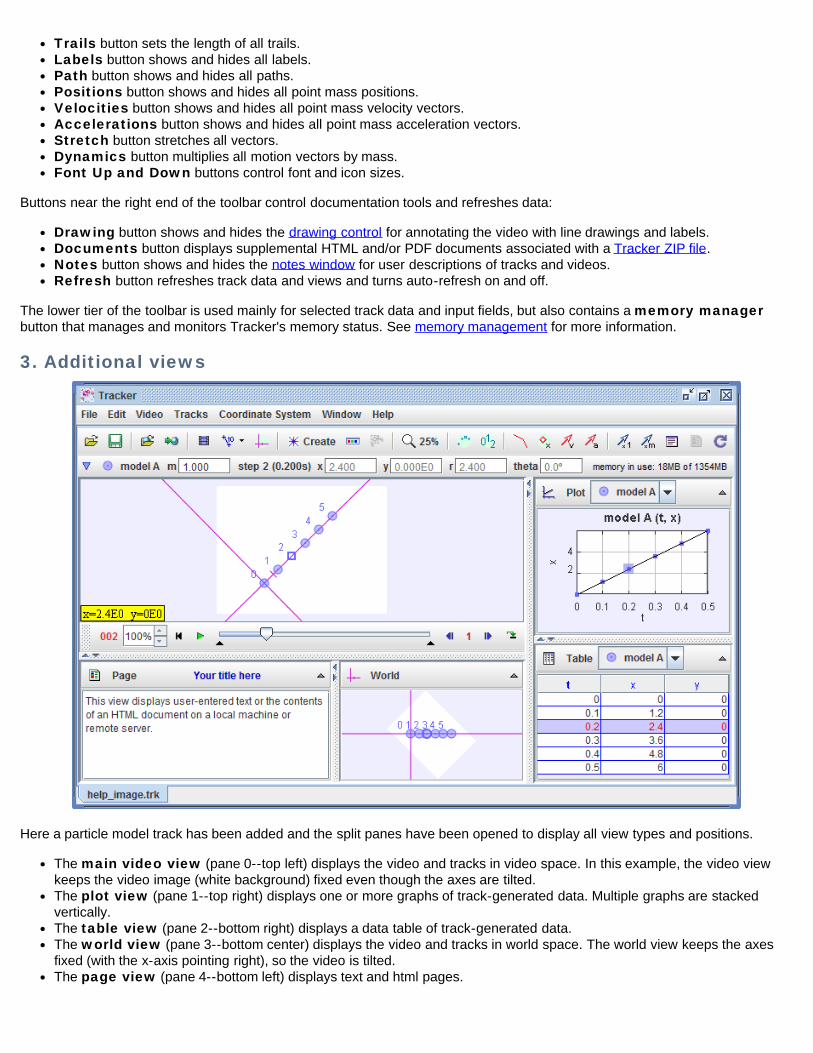
3. Additional views

Here a particle model track has been added and the split panes have been opened to display all view types and positions.

The main video view (pane 0--top left) displays the video and tracks in video space. In this example, the video viewkeeps the video image (white background) fixed even though the axes are tilted.The plot view (pane 1--top right) displays one or more graphs of track-generated data. Multiple graphs are stackedvertically.The table view (pane 2--bottom right) displays a data table of track-generated data.The world view (pane 3--bottom center) displays the video and tracks in world space. The world view keeps the axesfixed (with the x-axis pointing right), so the video is tilted.The page view (pane 4--bottom left) displays text and html pages.

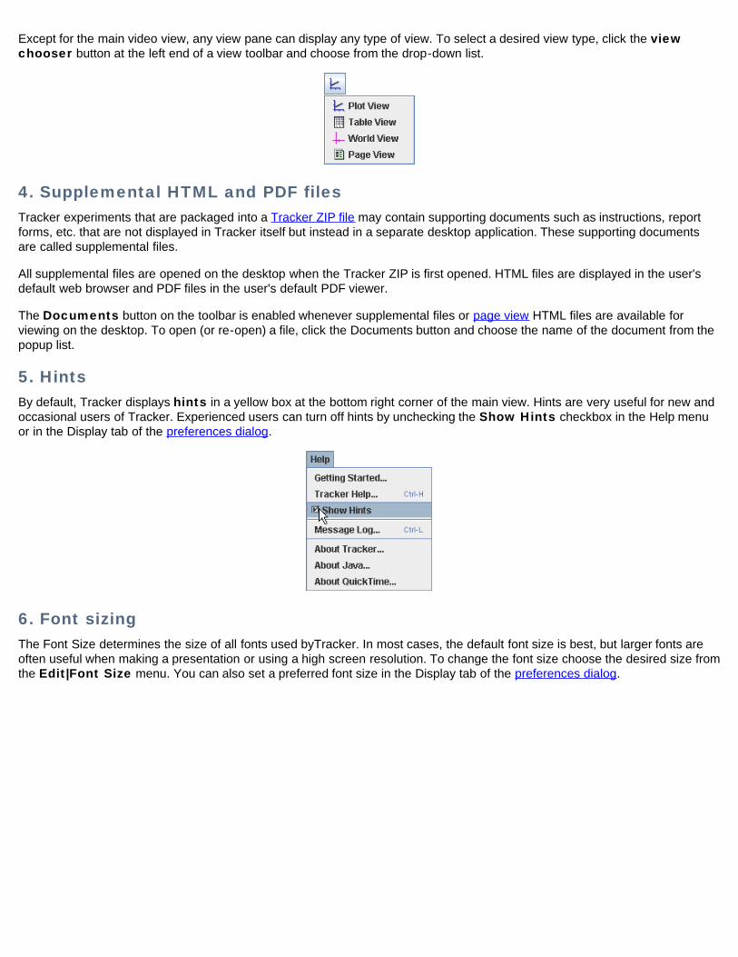
Except for the main video view, any view pane can display any type of view. To select a desired view type, click the viewchooser button at the left end of a view toolbar and choose from the drop-down list.

4. Supplemental HTML and PDF filesTracker experiments that are packaged into a Tracker ZIP file may contain supporting documents such as instructions, reportforms, etc. that are not displayed in Tracker itself but instead in a separate desktop application. These supporting documentsare called supplemental files.

All supplemental files are opened on the desktop when the Tracker ZIP is first opened. HTML files are displayed in the user'sdefault web browser and PDF files in the user's default PDF viewer.

The Documents button on the toolbar is enabled whenever supplemental files or page view HTML files are available forviewing on the desktop. To open (or re-open) a file, click the Documents button and choose the name of the document from thepopup list.

5. HintsBy default, Tracker displays hints in a yellow box at the bottom right corner of the main view. Hints are very useful for new andoccasional users of Tracker. Experienced users can turn off hints by unchecking the Show Hints checkbox in the Help menuor in the Display tab of the preferences dialog.

6. Font sizingThe Font Size determines the size of all fonts used byTracker. In most cases, the default font size is best, but larger fonts areoften useful when making a presentation or using a high screen resolution. To change the font size choose the desired size fromthe Edit|Font Size menu. You can also set a preferred font size in the Display tab of the preferences dialog.

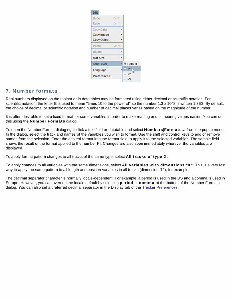
7. Number formatsReal numbers displayed on the toolbar or in datatables may be formatted using either decimal or scientific notation. Forscientific notation, the letter E is used to mean "times 10 to the power of" so the number 1.3 x 10^3 is written 1.3E3. By default,the choice of decimal or scientific notation and number of decimal places varies based on the magnitude of the number.

It is often desirable to set a fixed format for some variables in order to make reading and comparing values easier. You can dothis using the Number Formats dialog.

To open the Number Format dialog right-click a text field or datatable and select Numbers|Formats... from the popup menu.In the dialog, select the track and names of the variables you wish to format. Use the shift and control keys to add or removenames from the selection. Enter the desired format into the format field to apply it to the selected variables. The sample fieldshows the result of the format applied to the number PI. Changes are also seen immediately wherever the variables aredisplayed.

To apply format pattern changes to all tracks of the same type, select All tracks of type X.

To apply changes to all variables with the same dimensions, select All variables with dimensions "X". This is a very fastway to apply the same pattern to all length and position variables in all tracks (dimension "L"), for example.

The decimal separator character is normally locale-dependent. For example, a period is used in the US and a comma is used inEurope. However, you can override the locale default by selecting period or comma at the bottom of the Number Formatsdialog. You can also set a preferred decimal separator in the Display tab of the Tracker Preferences.

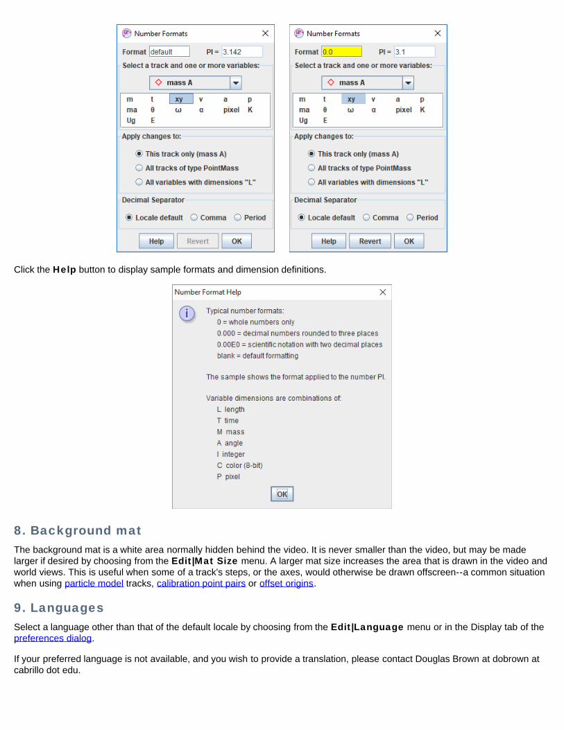
Click the Help button to display sample formats and dimension definitions.

8. Background matThe background mat is a white area normally hidden behind the video. It is never smaller than the video, but may be madelarger if desired by choosing from the Edit|Mat Size menu. A larger mat size increases the area that is drawn in the video andworld views. This is useful when some of a track's steps, or the axes, would otherwise be drawn offscreen--a common situationwhen using particle model tracks, calibration point pairs or offset origins.

9. LanguagesSelect a language other than that of the default locale by choosing from the Edit|Language menu or in the Display tab of thepreferences dialog.

If your preferred language is not available, and you wish to provide a translation, please contact Douglas Brown at dobrown atcabrillo dot edu.

10. Undo and redoMost operations in Tracker can be undone and redone using the Undo and Redo items in the Edit menu. There is no limit tothe number of undo actions.

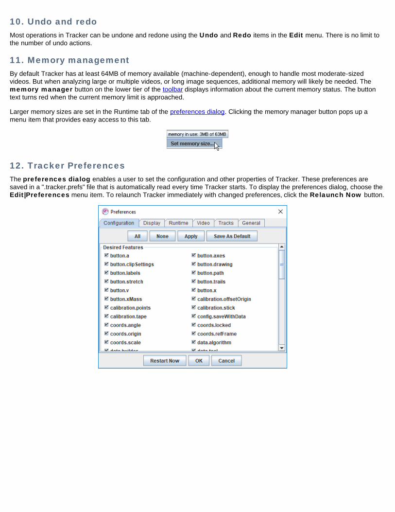
11. Memory managementBy default Tracker has at least 64MB of memory available (machine-dependent), enough to handle most moderate-sizedvideos. But when analyzing large or multiple videos, or long image sequences, additional memory will likely be needed. Thememory manager button on the lower tier of the toolbar displays information about the current memory status. The buttontext turns red when the current memory limit is approached.

Larger memory sizes are set in the Runtime tab of the preferences dialog. Clicking the memory manager button pops up amenu item that provides easy access to this tab.

12. Tracker PreferencesThe preferences dialog enables a user to set the configuration and other properties of Tracker. These preferences aresaved in a ".tracker.prefs" file that is automatically read every time Tracker starts. To display the preferences dialog, choose theEdit|Preferences menu item. To relaunch Tracker immediately with changed preferences, click the Relaunch Now button.

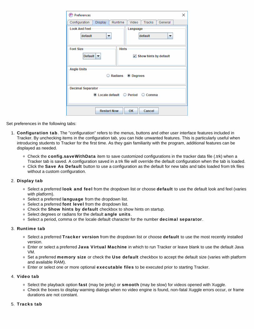
Set preferences in the following tabs:

1. Configuration tab. The "configuration" refers to the menus, buttons and other user interface features included inTracker. By unchecking items in the configuration tab, you can hide unwanted features. This is particularly useful whenintroducing students to Tracker for the first time. As they gain familiarity with the program, additional features can bedisplayed as needed.

Check the config.saveWithData item to save customized configurations in the tracker data file (.trk) when aTracker tab is saved. A configuration saved in a trk file will override the default configuration when the tab is loaded.Click the Save As Default button to use a configuration as the default for new tabs and tabs loaded from trk fileswithout a custom configuration.

2. Display tab

Select a preferred look and feel from the dropdown list or choose default to use the default look and feel (varieswith platform).Select a preferred language from the dropdown list.Select a preferred font level from the dropdown list.Check the Show hints by default checkbox to show hints on startup.Select degrees or radians for the default angle units.Select a period, comma or the locale default character for the number decimal separator.

3. Runtime tab

Select a preferred Tracker version from the dropdown list or choose default to use the most recently installedversion.Enter or select a preferred Java Virtual Machine in which to run Tracker or leave blank to use the default JavaVM.Set a preferred memory size or check the Use default checkbox to accept the default size (varies with platformand available RAM).Enter or select one or more optional executable files to be executed prior to starting Tracker.

4. Video tab

Select the playback option fast (may be jerky) or smooth (may be slow) for videos opened with Xuggle.Check the boxes to display warning dialogs when no video engine is found, non-fatal Xuggle errors occur, or framedurations are not constant.

5. Tracks tab

Check the box to auto-reset the video to step 0 when creating a new point mass, vector or rgb region.

6. General tab

Set the preferred number of files displayed in the File|Open Recent menu, or clear the current menu items.Set a preferred cache directory for downloaded web files, browse the cache in a file browser, or clear some or allcache files.Set the startup level for the Message Log. Set the level to ALL for detailed trouble-shooting.Select a preferred interval to automatically check for upgrades or click the Check Now button to checkimmediately.

VideosTracker can analyze three different video types:

1. digital video files (.mov, .avi, .mp4, .flv, .wmv, .ogg, etc.) which require a video engine (see below).2. animated GIF files (.gif).3. image sequences consisting of one or more digital images (.jpg, .png or pasted from the clipboard).

Tracker uses the Xuggle video engine to open most digital video files including .mov, .avi and .mp4 on all platforms.

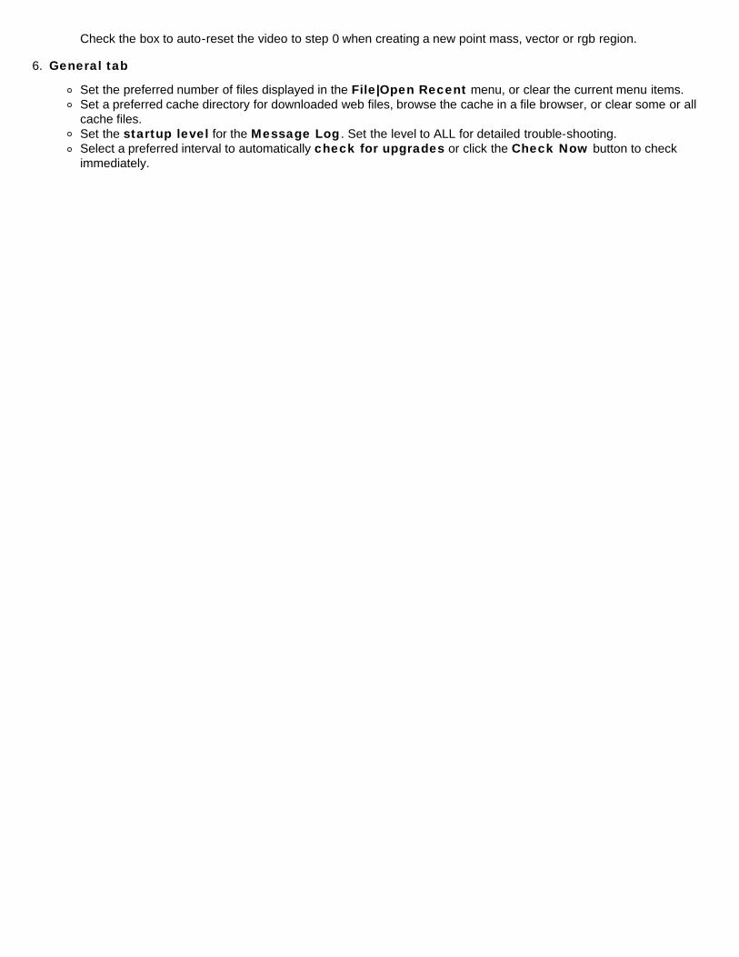
1. Opening or importing a video from a local driveTo open a video into a new tab, use the Open button or File|Open File menu item. To import a video into anexisting tab, use the Video|Import, Video|Replace or File|Import|Video menu item.

Select the desired video in the file chooser to open it.

2. Opening a video from the webChoose the File|Open URL menu item and enter a known URL in the dialog to open a video directly from the web.

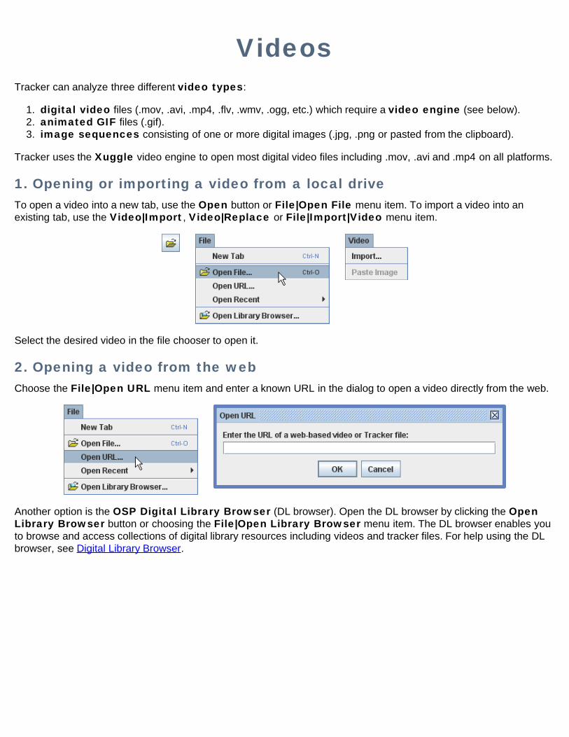
Another option is the OSP Digital Library Browser (DL browser). Open the DL browser by clicking the OpenLibrary Browser button or choosing the File|Open Library Browser menu item. The DL browser enables youto browse and access collections of digital library resources including videos and tracker files. For help using the DLbrowser, see Digital Library Browser.

3. Opening numbered image sequences ("image videos")Tracker will automatically open a sequence of up to 1000 JPG or PNG images that are numbered sequentially. Toopen a sequence, select only the first image in the sequence.

Image sequence numbering must have a fixed format. For example, selecting the first image in a sequence numberedimage00.jpg to image14.jpg will open all 15 images, but if the sequence is numbered image0.jpg to image14.jpg thenonly the first 10 images will be opened (i.e., up to image9.jpg).

Image videos loaded from files are initially read-only--each image file is loaded only when displayed. For fasterresponse and editing capabilities, you can load all images into memory by checking the "Load All Images" checkboxin the Video menu. Note: loading all images may require a great deal of memory; you can increase your availablememory in the preferences dialog.

4. Pasting images from the clipboardImages that have been copied to the clipboard may be pasted directly into Tracker for analysis. Choose theVideo|Paste Image or Video|Paste Image|Replace Video menu item to create a new image video.

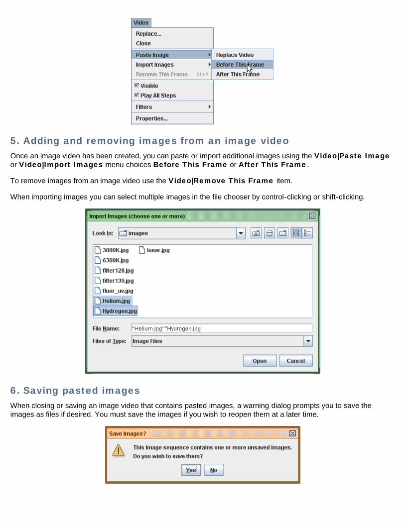
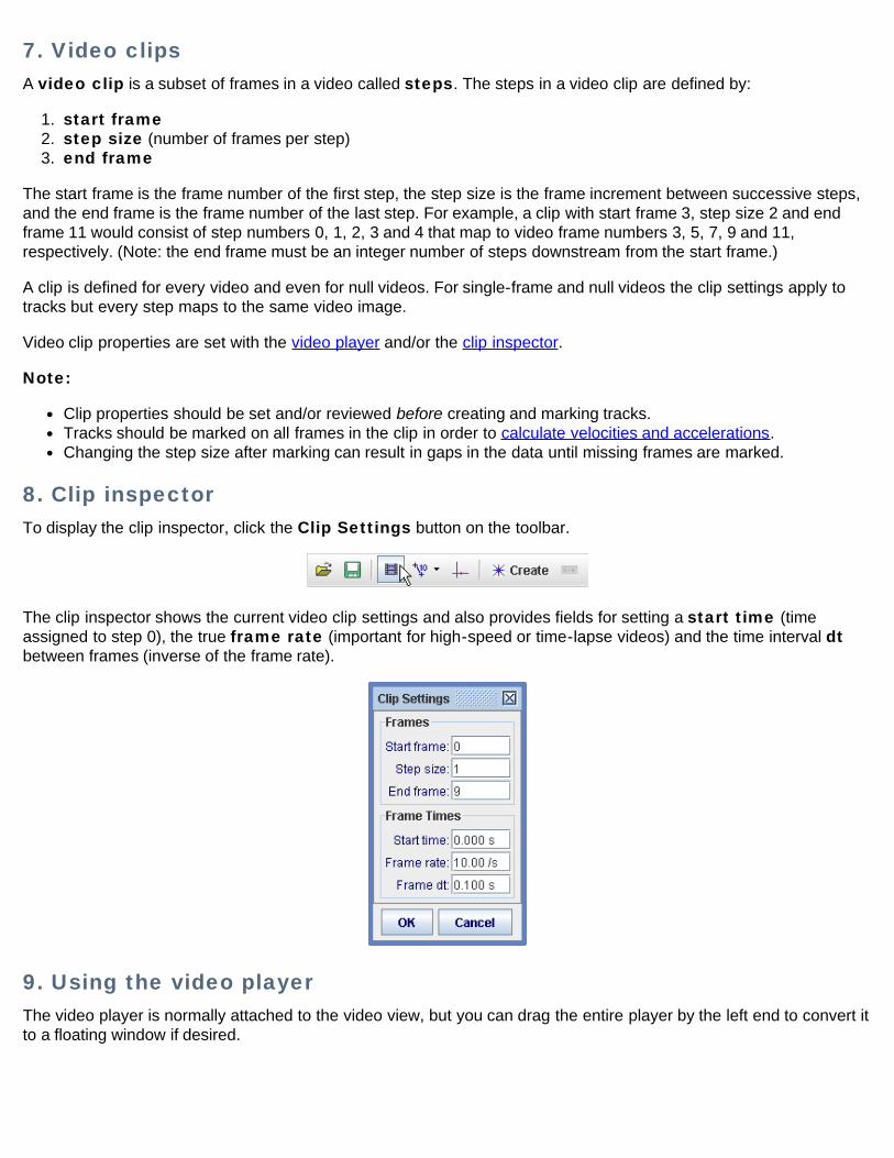
5. Adding and removing images from an image videoOnce an image video has been created, you can paste or import additional images using the Video|Paste Imageor Video|Import Images menu choices Before This Frame or After This Frame.

To remove images from an image video use the Video|Remove This Frame item.

When importing images you can select multiple images in the file chooser by control-clicking or shift-clicking.

6. Saving pasted imagesWhen closing or saving an image video that contains pasted images, a warning dialog prompts you to save theimages as files if desired. You must save the images if you wish to reopen them at a later time.

7. Video clipsA video clip is a subset of frames in a video called steps. The steps in a video clip are defined by:

1. start frame2. step size (number of frames per step)3. end frame

The start frame is the frame number of the first step, the step size is the frame increment between successive steps,and the end frame is the frame number of the last step. For example, a clip with start frame 3, step size 2 and endframe 11 would consist of step numbers 0, 1, 2, 3 and 4 that map to video frame numbers 3, 5, 7, 9 and 11,respectively. (Note: the end frame must be an integer number of steps downstream from the start frame.)

A clip is defined for every video and even for null videos. For single-frame and null videos the clip settings apply totracks but every step maps to the same video image.

Video clip properties are set with the video player and/or the clip inspector.

Note:

Clip properties should be set and/or reviewed before creating and marking tracks.Tracks should be marked on all frames in the clip in order to calculate velocities and accelerations.Changing the step size after marking can result in gaps in the data until missing frames are marked.

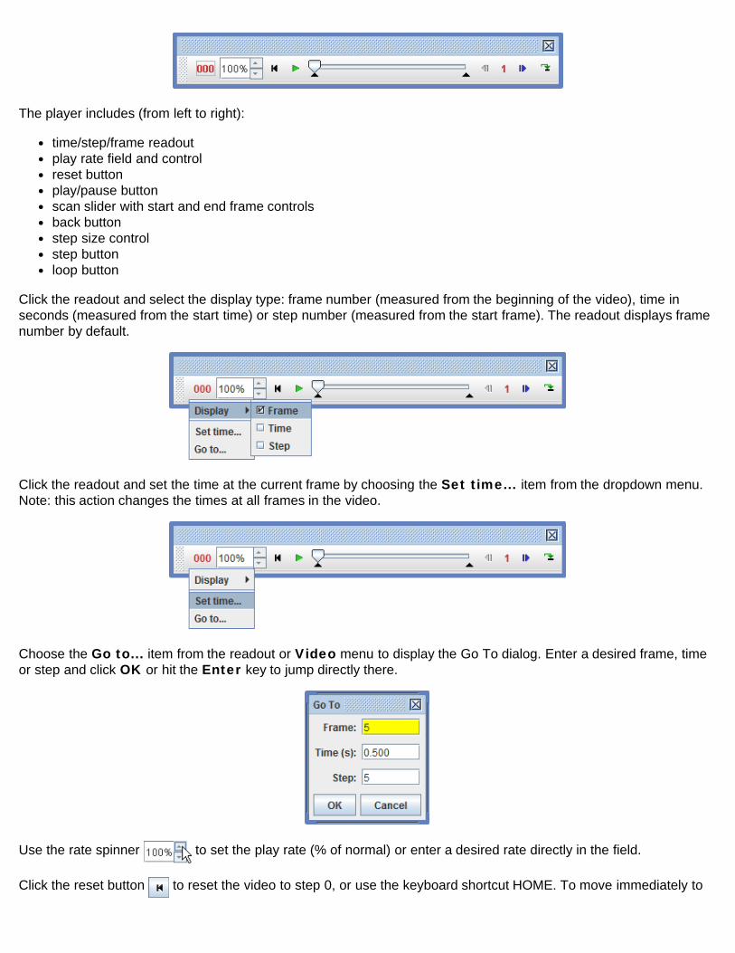
8. Clip inspectorTo display the clip inspector, click the Clip Settings button on the toolbar.

The clip inspector shows the current video clip settings and also provides fields for setting a start time (timeassigned to step 0), the true frame rate (important for high-speed or time-lapse videos) and the time interval dtbetween frames (inverse of the frame rate).

9. Using the video playerThe video player is normally attached to the video view, but you can drag the entire player by the left end to convert itto a floating window if desired.

The player includes (from left to right):

time/step/frame readoutplay rate field and controlreset buttonplay/pause buttonscan slider with start and end frame controlsback buttonstep size controlstep buttonloop button

Click the readout and select the display type: frame number (measured from the beginning of the video), time inseconds (measured from the start time) or step number (measured from the start frame). The readout displays framenumber by default.

Click the readout and set the time at the current frame by choosing the Set time... item from the dropdown menu.Note: this action changes the times at all frames in the video.

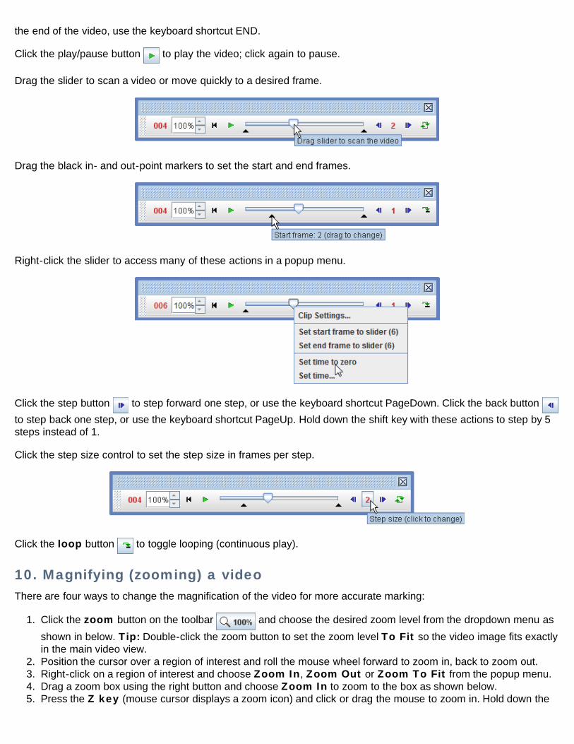
Choose the Go to... item from the readout or Video menu to display the Go To dialog. Enter a desired frame, timeor step and click OK or hit the Enter key to jump directly there.

Use the rate spinner to set the play rate (% of normal) or enter a desired rate directly in the field.

Click the reset button to reset the video to step 0, or use the keyboard shortcut HOME. To move immediately to

the end of the video, use the keyboard shortcut END.

Click the play/pause button to play the video; click again to pause.

Drag the slider to scan a video or move quickly to a desired frame.

Drag the black in- and out-point markers to set the start and end frames.

Right-click the slider to access many of these actions in a popup menu.

Click the step button to step forward one step, or use the keyboard shortcut PageDown. Click the back button to step back one step, or use the keyboard shortcut PageUp. Hold down the shift key with these actions to step by 5steps instead of 1.

Click the step size control to set the step size in frames per step.

Click the loop button to toggle looping (continuous play).

10. Magnifying (zooming) a videoThere are four ways to change the magnification of the video for more accurate marking:

1. Click the zoom button on the toolbar and choose the desired zoom level from the dropdown menu asshown in below. Tip: Double-click the zoom button to set the zoom level To Fit so the video image fits exactlyin the main video view.

2. Position the cursor over a region of interest and roll the mouse wheel forward to zoom in, back to zoom out.3. Right-click on a region of interest and choose Zoom In, Zoom Out or Zoom To Fit from the popup menu.4. Drag a zoom box using the right button and choose Zoom In to zoom to the box as shown below.5. Press the Z key (mouse cursor displays a zoom icon) and click or drag the mouse to zoom in. Hold down the

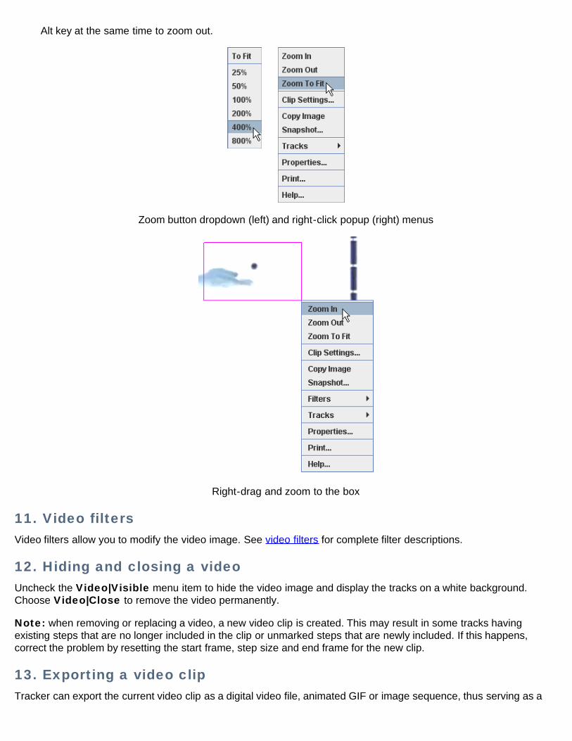
Alt key at the same time to zoom out.

Zoom button dropdown (left) and right-click popup (right) menus

Right-drag and zoom to the box

11. Video filtersVideo filters allow you to modify the video image. See video filters for complete filter descriptions.

12. Hiding and closing a videoUncheck the Video|Visible menu item to hide the video image and display the tracks on a white background.Choose Video|Close to remove the video permanently.

Note: when removing or replacing a video, a new video clip is created. This may result in some tracks havingexisting steps that are no longer included in the clip or unmarked steps that are newly included. If this happens,correct the problem by resetting the start frame, step size and end frame for the new clip.

13. Exporting a video clipTracker can export the current video clip as a digital video file, animated GIF or image sequence, thus serving as a

simple video editor and transcoder. But exported videos can also include track overlays, video filters, and additionalviews like world views and plots, making them useful for documenting the video modeling or analysis results.Interlaced 30 fps videos can also be exported as 60 fps deinterlaced videos, which doubles the temporal resolutionwhile halving the vertical resolution.

Note: the exported video contains only frames in the current video clip (determined by start frame, step size and endframe), not the entire video.

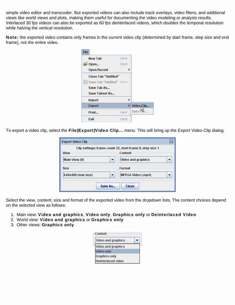
To export a video clip, select the File|Export|Video Clip... menu. This will bring up the Export Video Clip dialog.

Select the view, content, size and format of the exported video from the dropdown lists. The content choices dependon the selected view as follows:

1. Main view: Video and graphics, Video only, Graphics only or Deinterlaced Video2. World view: Video and graphics or Graphics only3. Other views: Graphics only

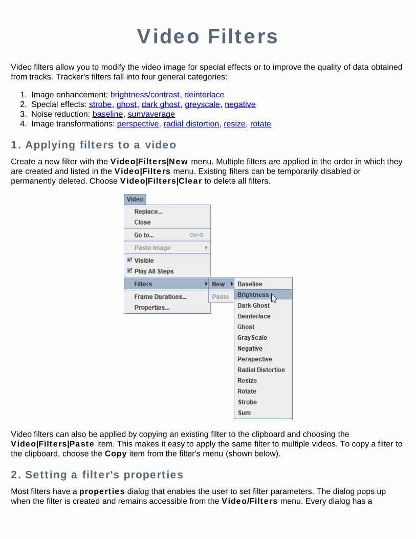
Video FiltersVideo filters allow you to modify the video image for special effects or to improve the quality of data obtainedfrom tracks. Tracker's filters fall into four general categories:

1. Image enhancement: brightness/contrast, deinterlace2. Special effects: strobe, ghost, dark ghost, greyscale, negative3. Noise reduction: baseline, sum/average4. Image transformations: perspective, radial distortion, resize, rotate

1. Applying filters to a videoCreate a new filter with the Video|Filters|New menu. Multiple filters are applied in the order in which theyare created and listed in the Video|Filters menu. Existing filters can be temporarily disabled orpermanently deleted. Choose Video|Filters|Clear to delete all filters.

Video filters can also be applied by copying an existing filter to the clipboard and choosing theVideo|Filters|Paste item. This makes it easy to apply the same filter to multiple videos. To copy a filter tothe clipboard, choose the Copy item from the filter's menu (shown below).

2. Setting a filter's propertiesMost filters have a properties dialog that enables the user to set filter parameters. The dialog pops upwhen the filter is created and remains accessible from the Video/Filters menu. Every dialog has a

Disable button that temporarily disables the filter so it has no effect.

3. Brightness/contrast filterThe brightness filter has adjustments for both brightness (range -128 to +128) and contrast (range 0-100).Changes in brightness affect the RGB components of all pixels equally until minimum (0) or maximum (255)values are reached.

To set a value, use the slider or enter it directly in a field. The Clear button resets the brightness andcontrast to their default values.

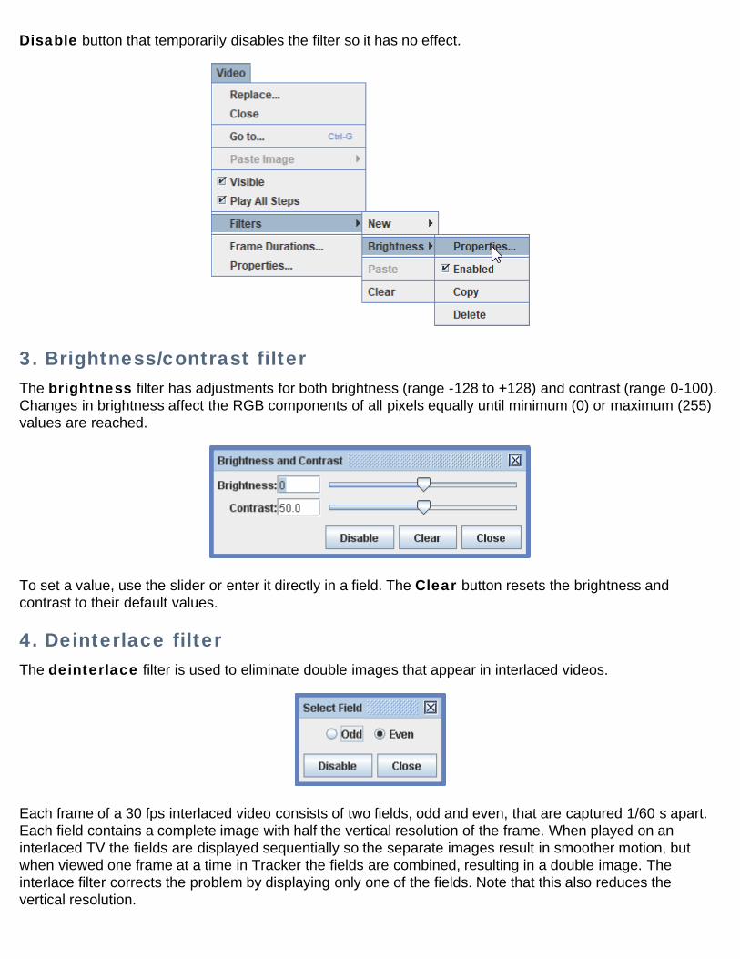
4. Deinterlace filterThe deinterlace filter is used to eliminate double images that appear in interlaced videos.

Each frame of a 30 fps interlaced video consists of two fields, odd and even, that are captured 1/60 s apart.Each field contains a complete image with half the vertical resolution of the frame. When played on aninterlaced TV the fields are displayed sequentially so the separate images result in smoother motion, butwhen viewed one frame at a time in Tracker the fields are combined, resulting in a double image. Theinterlace filter corrects the problem by displaying only one of the fields. Note that this also reduces thevertical resolution.

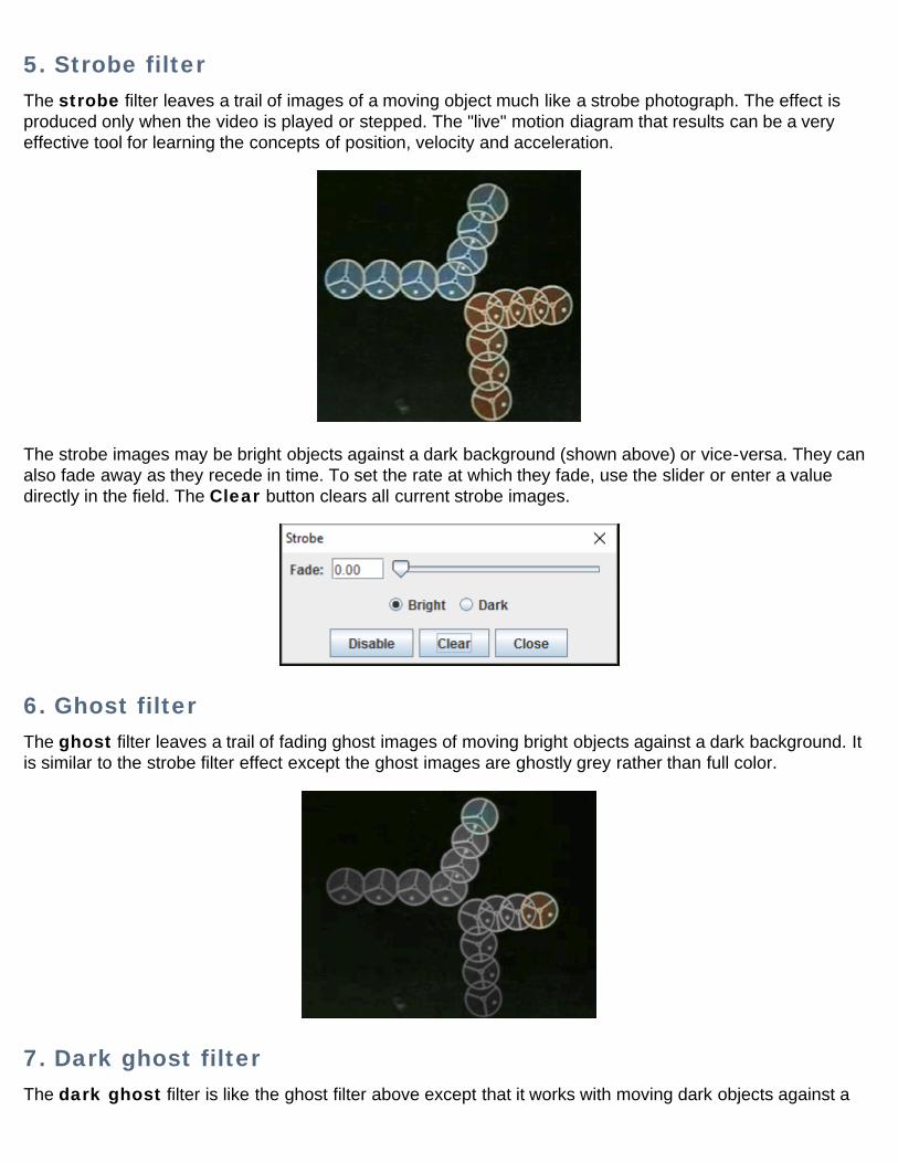
5. Strobe filterThe strobe filter leaves a trail of images of a moving object much like a strobe photograph. The effect isproduced only when the video is played or stepped. The "live" motion diagram that results can be a veryeffective tool for learning the concepts of position, velocity and acceleration.

The strobe images may be bright objects against a dark background (shown above) or vice-versa. They canalso fade away as they recede in time. To set the rate at which they fade, use the slider or enter a valuedirectly in the field. The Clear button clears all current strobe images.

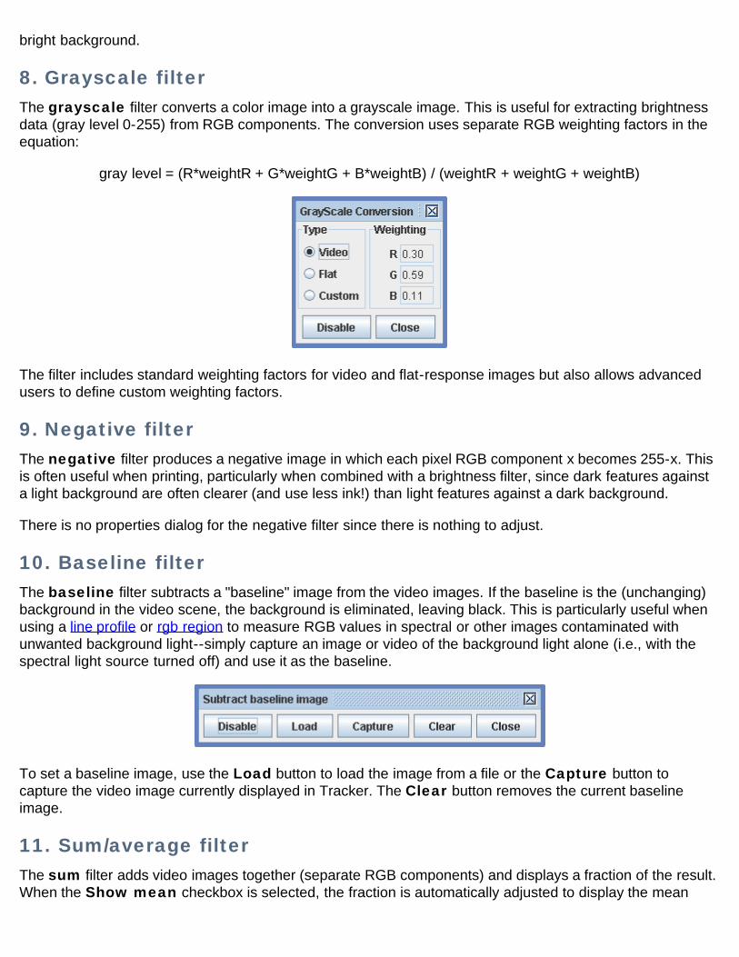
6. Ghost filterThe ghost filter leaves a trail of fading ghost images of moving bright objects against a dark background. Itis similar to the strobe filter effect except the ghost images are ghostly grey rather than full color.

7. Dark ghost filterThe dark ghost filter is like the ghost filter above except that it works with moving dark objects against a

bright background.

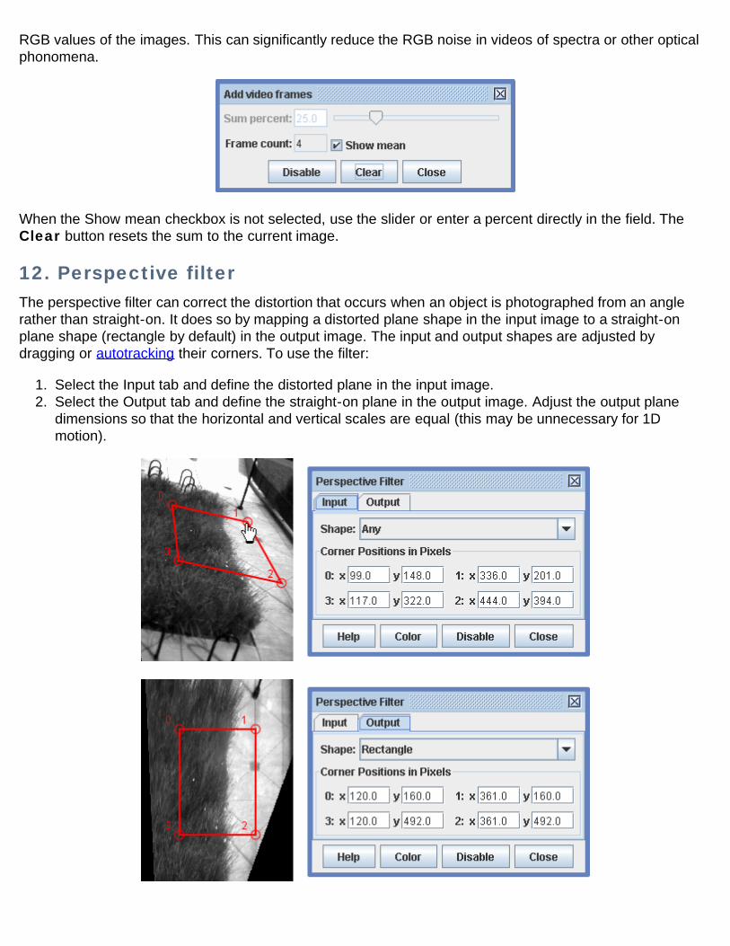
8. Grayscale filterThe grayscale filter converts a color image into a grayscale image. This is useful for extracting brightnessdata (gray level 0-255) from RGB components. The conversion uses separate RGB weighting factors in theequation:

gray level = (R*weightR + G*weightG + B*weightB) / (weightR + weightG + weightB)

The filter includes standard weighting factors for video and flat-response images but also allows advancedusers to define custom weighting factors.

9. Negative filterThe negative filter produces a negative image in which each pixel RGB component x becomes 255-x. Thisis often useful when printing, particularly when combined with a brightness filter, since dark features againsta light background are often clearer (and use less ink!) than light features against a dark background.

There is no properties dialog for the negative filter since there is nothing to adjust.

10. Baseline filterThe baseline filter subtracts a "baseline" image from the video images. If the baseline is the (unchanging)background in the video scene, the background is eliminated, leaving black. This is particularly useful whenusing a line profile or rgb region to measure RGB values in spectral or other images contaminated withunwanted background light--simply capture an image or video of the background light alone (i.e., with thespectral light source turned off) and use it as the baseline.

To set a baseline image, use the Load button to load the image from a file or the Capture button tocapture the video image currently displayed in Tracker. The Clear button removes the current baselineimage.

11. Sum/average filterThe sum filter adds video images together (separate RGB components) and displays a fraction of the result.When the Show mean checkbox is selected, the fraction is automatically adjusted to display the mean

RGB values of the images. This can significantly reduce the RGB noise in videos of spectra or other opticalphonomena.

When the Show mean checkbox is not selected, use the slider or enter a percent directly in the field. TheClear button resets the sum to the current image.

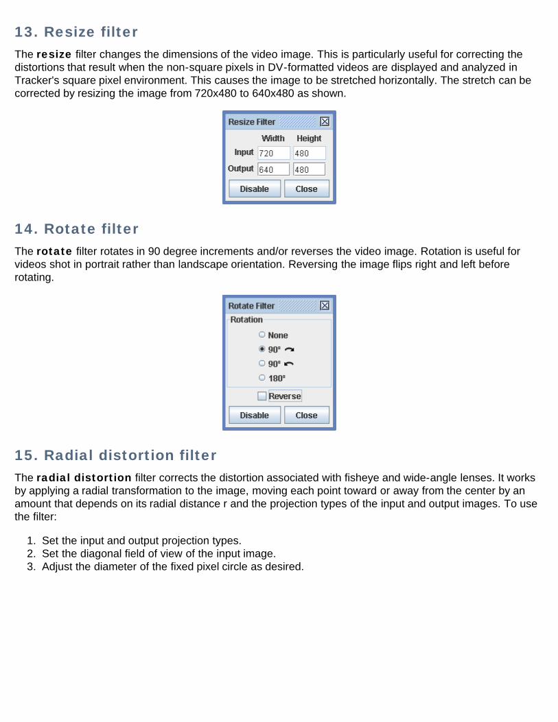
12. Perspective filterThe perspective filter can correct the distortion that occurs when an object is photographed from an anglerather than straight-on. It does so by mapping a distorted plane shape in the input image to a straight-onplane shape (rectangle by default) in the output image. The input and output shapes are adjusted bydragging or autotracking their corners. To use the filter:

1. Select the Input tab and define the distorted plane in the input image.2. Select the Output tab and define the straight-on plane in the output image. Adjust the output plane

dimensions so that the horizontal and vertical scales are equal (this may be unnecessary for 1Dmotion).

13. Resize filterThe resize filter changes the dimensions of the video image. This is particularly useful for correcting thedistortions that result when the non-square pixels in DV-formatted videos are displayed and analyzed inTracker's square pixel environment. This causes the image to be stretched horizontally. The stretch can becorrected by resizing the image from 720x480 to 640x480 as shown.

14. Rotate filterThe rotate filter rotates in 90 degree increments and/or reverses the video image. Rotation is useful forvideos shot in portrait rather than landscape orientation. Reversing the image flips right and left beforerotating.

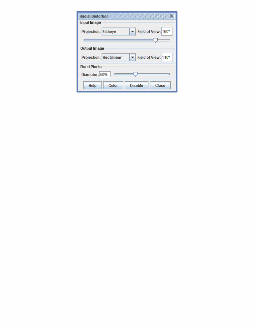
15. Radial distortion filterThe radial distortion filter corrects the distortion associated with fisheye and wide-angle lenses. It worksby applying a radial transformation to the image, moving each point toward or away from the center by anamount that depends on its radial distance r and the projection types of the input and output images. To usethe filter:

1. Set the input and output projection types.2. Set the diagonal field of view of the input image.3. Adjust the diameter of the fixed pixel circle as desired.

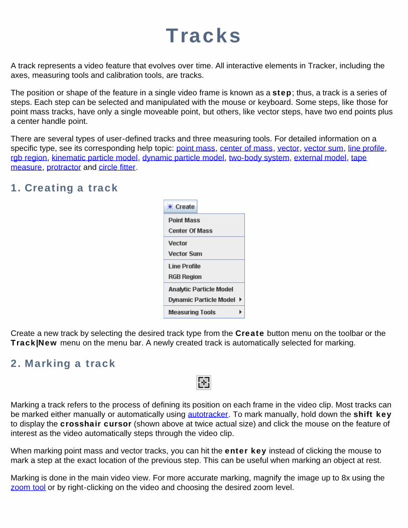
TracksA track represents a video feature that evolves over time. All interactive elements in Tracker, including theaxes, measuring tools and calibration tools, are tracks.

The position or shape of the feature in a single video frame is known as a step; thus, a track is a series ofsteps. Each step can be selected and manipulated with the mouse or keyboard. Some steps, like those forpoint mass tracks, have only a single moveable point, but others, like vector steps, have two end points plusa center handle point.

There are several types of user-defined tracks and three measuring tools. For detailed information on aspecific type, see its corresponding help topic: point mass, center of mass, vector, vector sum, line profile,rgb region, kinematic particle model, dynamic particle model, two-body system, external model, tapemeasure, protractor and circle fitter.

1. Creating a track

Create a new track by selecting the desired track type from the Create button menu on the toolbar or theTrack|New menu on the menu bar. A newly created track is automatically selected for marking.

2. Marking a track

Marking a track refers to the process of defining its position on each frame in the video clip. Most tracks canbe marked either manually or automatically using autotracker. To mark manually, hold down the shift keyto display the crosshair cursor (shown above at twice actual size) and click the mouse on the feature ofinterest as the video automatically steps through the video clip.

When marking point mass and vector tracks, you can hit the enter key instead of clicking the mouse tomark a step at the exact location of the previous step. This can be useful when marking an object at rest.

Marking is done in the main video view. For more accurate marking, magnify the image up to 8x using thezoom tool or by right-clicking on the video and choosing the desired zoom level.

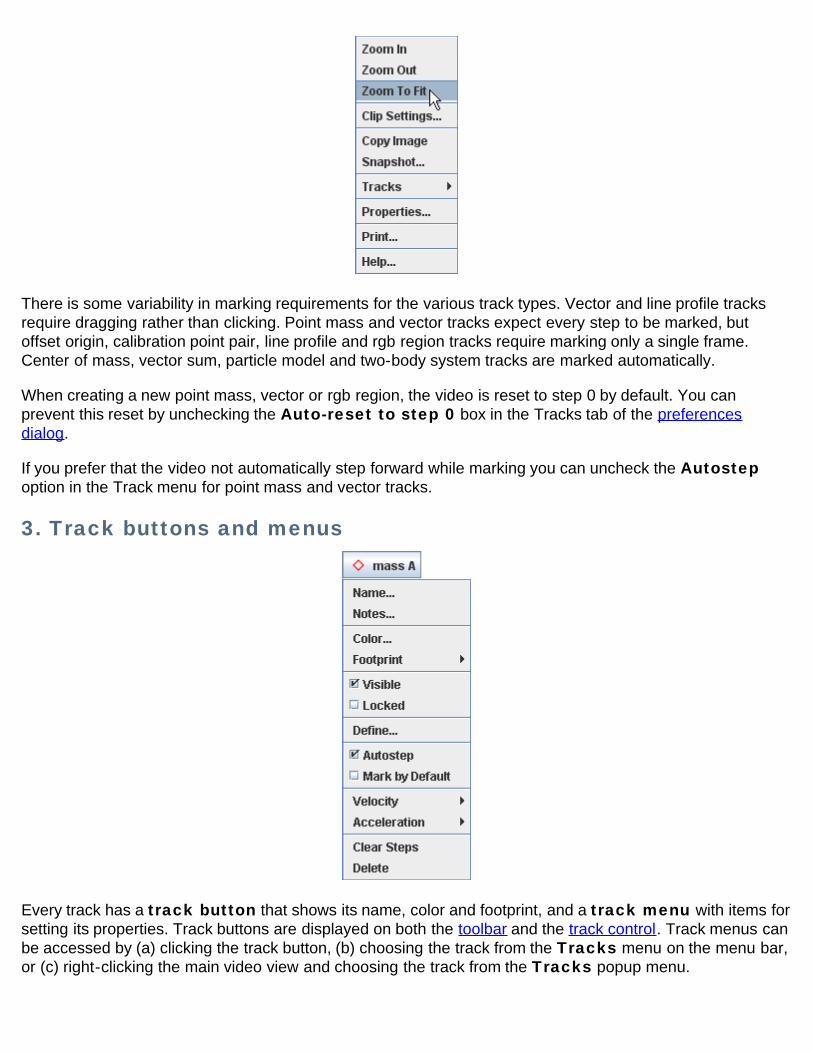
There is some variability in marking requirements for the various track types. Vector and line profile tracksrequire dragging rather than clicking. Point mass and vector tracks expect every step to be marked, butoffset origin, calibration point pair, line profile and rgb region tracks require marking only a single frame.Center of mass, vector sum, particle model and two-body system tracks are marked automatically.

When creating a new point mass, vector or rgb region, the video is reset to step 0 by default. You canprevent this reset by unchecking the Auto-reset to step 0 box in the Tracks tab of the preferencesdialog.

If you prefer that the video not automatically step forward while marking you can uncheck the Autostepoption in the Track menu for point mass and vector tracks.

3. Track buttons and menus

Every track has a track button that shows its name, color and footprint, and a track menu with items forsetting its properties. Track buttons are displayed on both the toolbar and the track control. Track menus canbe accessed by (a) clicking the track button, (b) choosing the track from the Tracks menu on the menu bar,or (c) right-clicking the main video view and choosing the track from the Tracks popup menu.

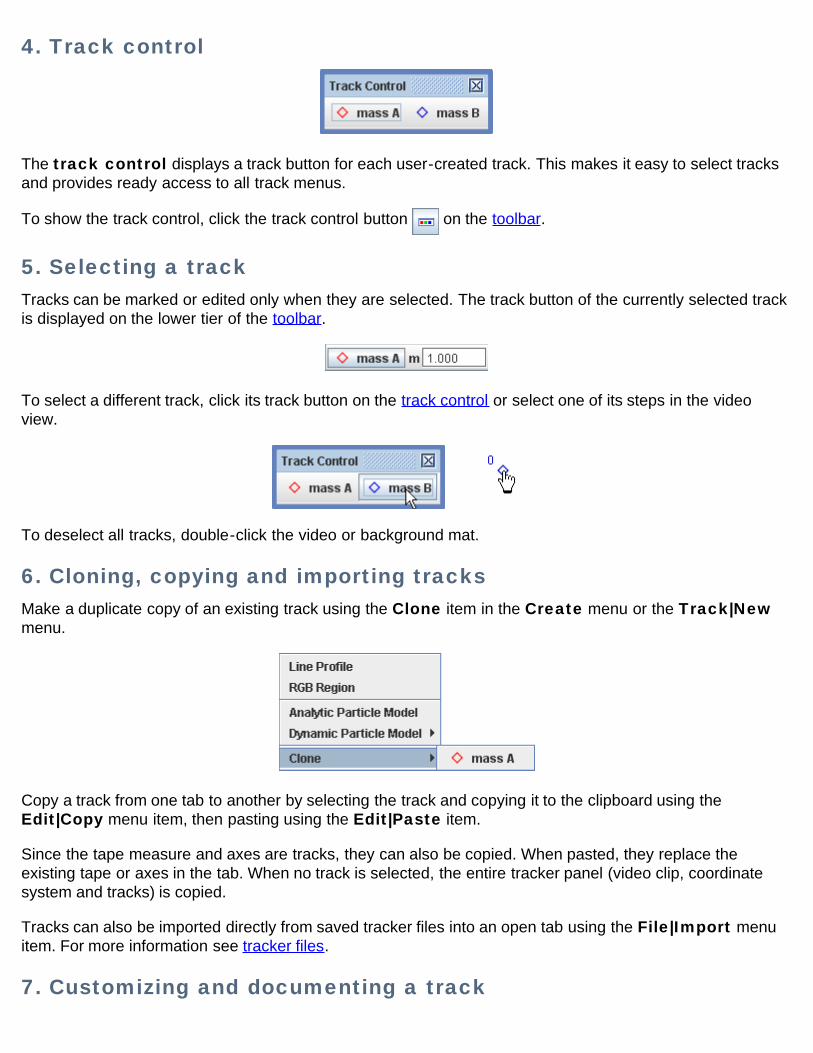
4. Track control

The track control displays a track button for each user-created track. This makes it easy to select tracksand provides ready access to all track menus.

To show the track control, click the track control button on the toolbar.

5. Selecting a trackTracks can be marked or edited only when they are selected. The track button of the currently selected trackis displayed on the lower tier of the toolbar.

To select a different track, click its track button on the track control or select one of its steps in the videoview.

To deselect all tracks, double-click the video or background mat.

6. Cloning, copying and importing tracksMake a duplicate copy of an existing track using the Clone item in the Create menu or the Track|Newmenu.

Copy a track from one tab to another by selecting the track and copying it to the clipboard using theEdit|Copy menu item, then pasting using the Edit|Paste item.

Since the tape measure and axes are tracks, they can also be copied. When pasted, they replace theexisting tape or axes in the tab. When no track is selected, the entire tracker panel (video clip, coordinatesystem and tracks) is copied.

Tracks can also be imported directly from saved tracker files into an open tab using the File|Import menuitem. For more information see tracker files.

7. Customizing and documenting a track

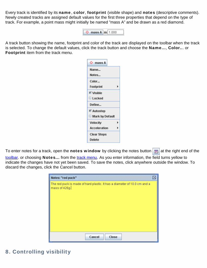
Every track is identified by its name, color, footprint (visible shape) and notes (descriptive comments).Newly created tracks are assigned default values for the first three properties that depend on the type oftrack. For example, a point mass might initially be named ”mass A” and be drawn as a red diamond.

A track button showing the name, footprint and color of the track are displayed on the toolbar when the trackis selected. To change the default values, click the track button and choose the Name..., Color... orFootprint item from the track menu.

To enter notes for a track, open the notes window by clicking the notes button at the right end of thetoolbar. or choosing Notes... from the track menu. As you enter information, the field turns yellow toindicate the changes have not yet been saved. To save the notes, click anywhere outside the window. Todiscard the changes, click the Cancel button.

8. Controlling visibility

Hide a track by turning off the Visible property in its track menu. Or use the trails, labels, paths,positions, velocities and accelerations buttons on the toolbar to toggle the visibility of these featureson all tracks.

9. Selecting and identifying points

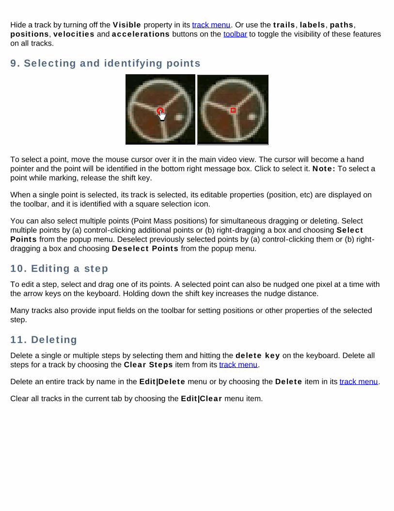
To select a point, move the mouse cursor over it in the main video view. The cursor will become a handpointer and the point will be identified in the bottom right message box. Click to select it. Note: To select apoint while marking, release the shift key.

When a single point is selected, its track is selected, its editable properties (position, etc) are displayed onthe toolbar, and it is identified with a square selection icon.

You can also select multiple points (Point Mass positions) for simultaneous dragging or deleting. Selectmultiple points by (a) control-clicking additional points or (b) right-dragging a box and choosing SelectPoints from the popup menu. Deselect previously selected points by (a) control-clicking them or (b) right-dragging a box and choosing Deselect Points from the popup menu.

10. Editing a stepTo edit a step, select and drag one of its points. A selected point can also be nudged one pixel at a time withthe arrow keys on the keyboard. Holding down the shift key increases the nudge distance.

Many tracks also provide input fields on the toolbar for setting positions or other properties of the selectedstep.

11. DeletingDelete a single or multiple steps by selecting them and hitting the delete key on the keyboard. Delete allsteps for a track by choosing the Clear Steps item from its track menu.

Delete an entire track by name in the Edit|Delete menu or by choosing the Delete item in its track menu.

Clear all tracks in the current tab by choosing the Edit|Clear menu item.

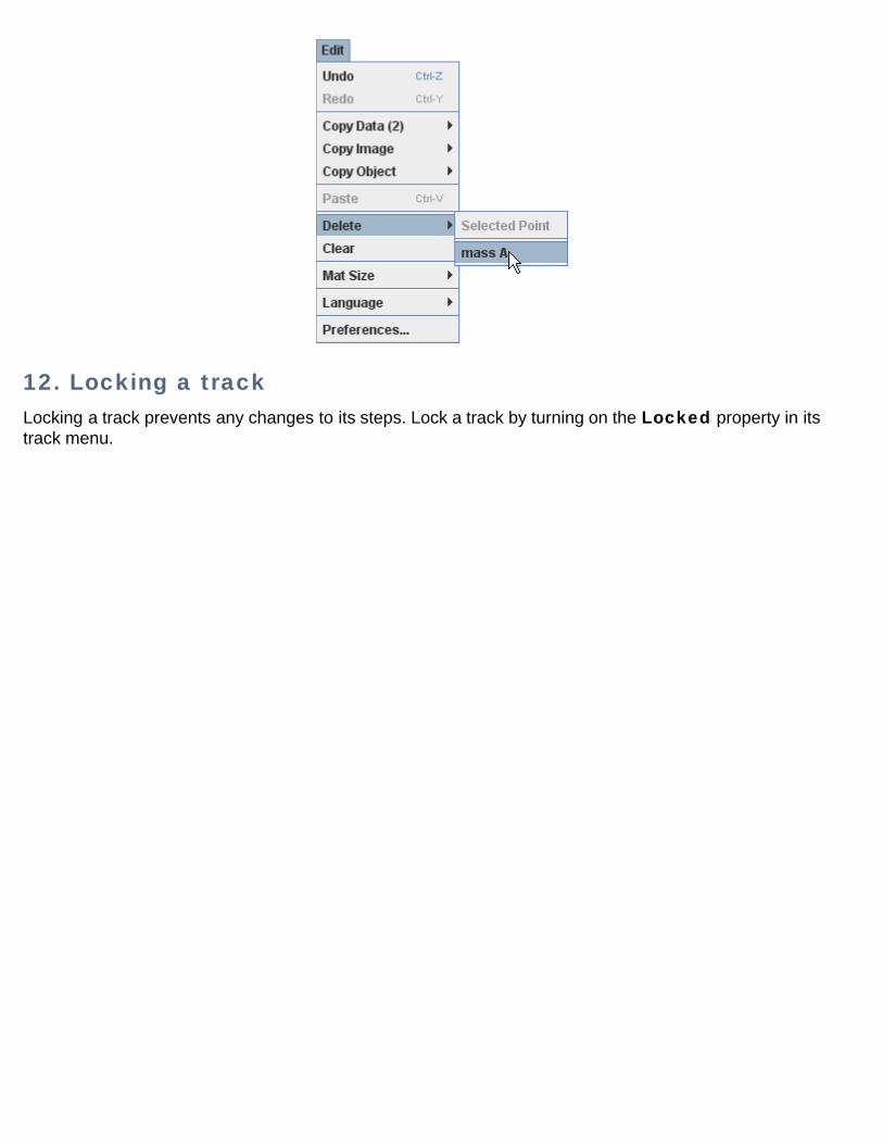
12. Locking a trackLocking a track prevents any changes to its steps. Lock a track by turning on the Locked property in itstrack menu.

Coordinate SystemWhen you mark a point in Tracker's main video view, you are defining its image position. Image positionsare measured in pixel units relative to the top left corner of the video image. In a 320 x 240 pixel image theupper left corner is at image position (0.0, 0.0) and the lower right is at (320.0, 240.0).

Since a video image is a camera view of the real world, a physical object within that image also has worldcoordinates. World coordinates are measured in scaled world units (e.g., meters) relative to a specifiedreference frame. The origin of the reference frame may be anywhere on or off the image.

The coordinate system is a set of transformations used to convert image positions into worldcoordinates. The coordinate system defines for each frame of the video:

scale (image units per world unit)origin (image position of the reference frame origin)angle (counterclockwise angle from the image x-axis to the world x-axis.

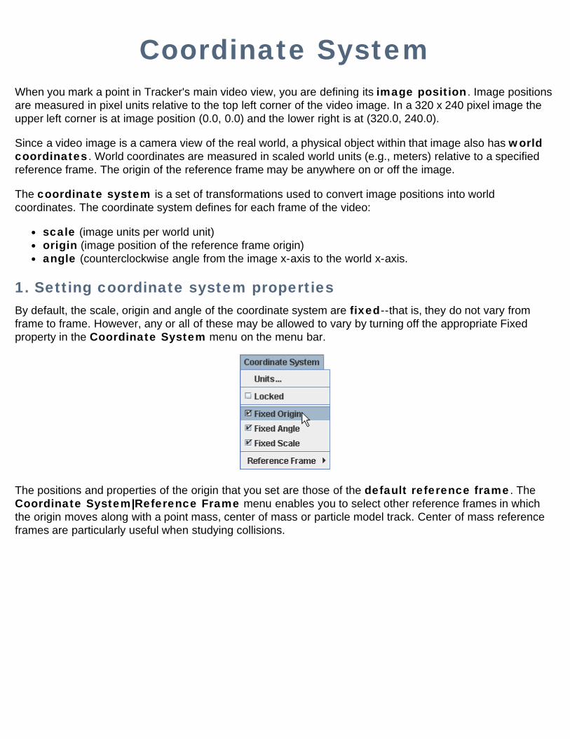
1. Setting coordinate system propertiesBy default, the scale, origin and angle of the coordinate system are fixed--that is, they do not vary fromframe to frame. However, any or all of these may be allowed to vary by turning off the appropriate Fixedproperty in the Coordinate System menu on the menu bar.

The positions and properties of the origin that you set are those of the default reference frame. TheCoordinate System|Reference Frame menu enables you to select other reference frames in whichthe origin moves along with a point mass, center of mass or particle model track. Center of mass referenceframes are particularly useful when studying collisions.

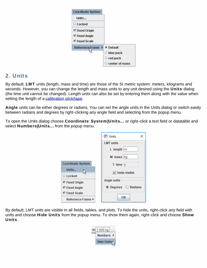
2. UnitsBy default, LMT units (length, mass and time) are those of the SI metric system: meters, kilograms andseconds. However, you can change the length and mass units to any unit desired using the Units dialog(the time unit cannot be changed). Length units can also be set by entering them along with the value whensetting the length of a calibration stick/tape.

Angle units can be either degrees or radians. You can set the angle units in the Units dialog or switch easilybetween radians and degrees by right-clicking any angle field and selecting from the popup menu.

To open the Units dialog choose Coordinate System|Units... or right-click a text field or datatable andselect Numbers|Units... from the popup menu.

By default, LMT units are visible in all fields, tables, and plots. To hide the units, right-click any field withunits and choose Hide Units from the popup menu. To show them again, right-click and choose ShowUnits.

3. Setting the scale (calibrating)Set the scale using a calibration stick/tape or calibration points.

4. Setting the originSet the position of the origin using the axes, an offset origin or calibration points.

5. Setting the angleSet the angle of the x-axis using the axes, calibration stick/tape or calibration points.

6. Locking the coordinate systemLocking the coordinate system prevents any changes to the scale, origin and angle. Lock it by turning on theLocked property in the Coordinate System menu.

Coordinate Axes

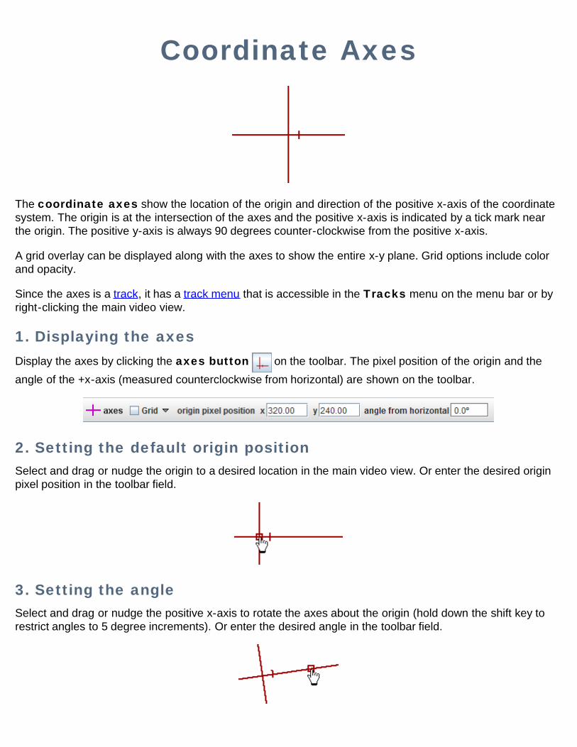
The coordinate axes show the location of the origin and direction of the positive x-axis of the coordinatesystem. The origin is at the intersection of the axes and the positive x-axis is indicated by a tick mark nearthe origin. The positive y-axis is always 90 degrees counter-clockwise from the positive x-axis.

A grid overlay can be displayed along with the axes to show the entire x-y plane. Grid options include colorand opacity.

Since the axes is a track, it has a track menu that is accessible in the Tracks menu on the menu bar or byright-clicking the main video view.

1. Displaying the axesDisplay the axes by clicking the axes button on the toolbar. The pixel position of the origin and theangle of the +x-axis (measured counterclockwise from horizontal) are shown on the toolbar.

2. Setting the default origin positionSelect and drag or nudge the origin to a desired location in the main video view. Or enter the desired originpixel position in the toolbar field.

3. Setting the angleSelect and drag or nudge the positive x-axis to rotate the axes about the origin (hold down the shift key torestrict angles to 5 degree increments). Or enter the desired angle in the toolbar field.

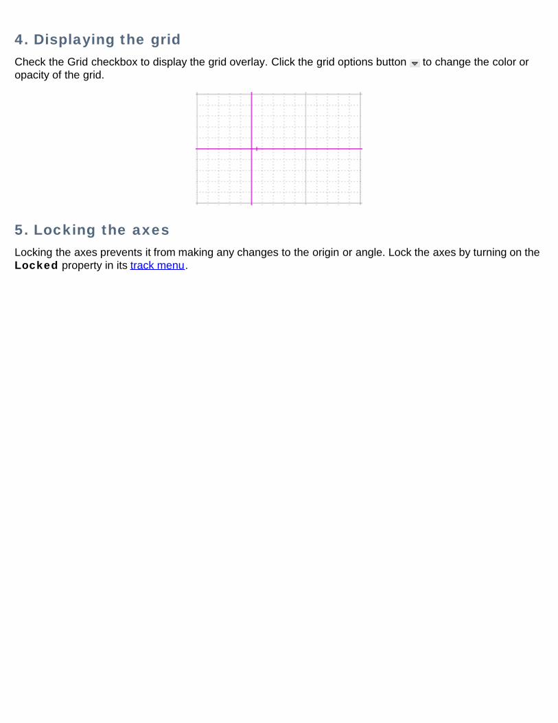
4. Displaying the gridCheck the Grid checkbox to display the grid overlay. Click the grid options button to change the color oropacity of the grid.

5. Locking the axesLocking the axes prevents it from making any changes to the origin or angle. Lock the axes by turning on theLocked property in its track menu.

Calibration Stick and Tape

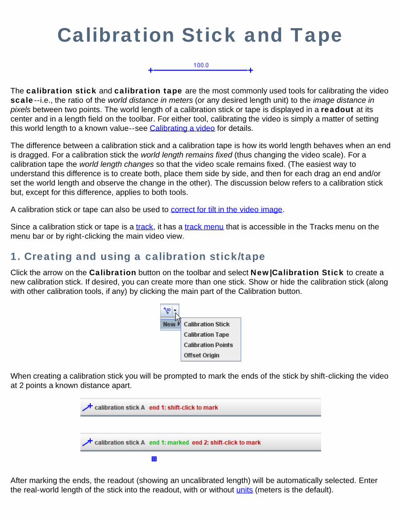
The calibration stick and calibration tape are the most commonly used tools for calibrating the videoscale--i.e., the ratio of the world distance in meters (or any desired length unit) to the image distance inpixels between two points. The world length of a calibration stick or tape is displayed in a readout at itscenter and in a length field on the toolbar. For either tool, calibrating the video is simply a matter of settingthis world length to a known value--see Calibrating a video for details.

The difference between a calibration stick and a calibration tape is how its world length behaves when an endis dragged. For a calibration stick the world length remains fixed (thus changing the video scale). For acalibration tape the world length changes so that the video scale remains fixed. (The easiest way tounderstand this difference is to create both, place them side by side, and then for each drag an end and/orset the world length and observe the change in the other). The discussion below refers to a calibration stickbut, except for this difference, applies to both tools.

A calibration stick or tape can also be used to correct for tilt in the video image.

Since a calibration stick or tape is a track, it has a track menu that is accessible in the Tracks menu on themenu bar or by right-clicking the main video view.

1. Creating and using a calibration stick/tapeClick the arrow on the Calibration button on the toolbar and select New|Calibration Stick to create anew calibration stick. If desired, you can create more than one stick. Show or hide the calibration stick (alongwith other calibration tools, if any) by clicking the main part of the Calibration button.

When creating a calibration stick you will be prompted to mark the ends of the stick by shift-clicking the videoat 2 points a known distance apart.

After marking the ends, the readout (showing an uncalibrated length) will be automatically selected. Enterthe real-world length of the stick into the readout, with or without units (meters is the default).

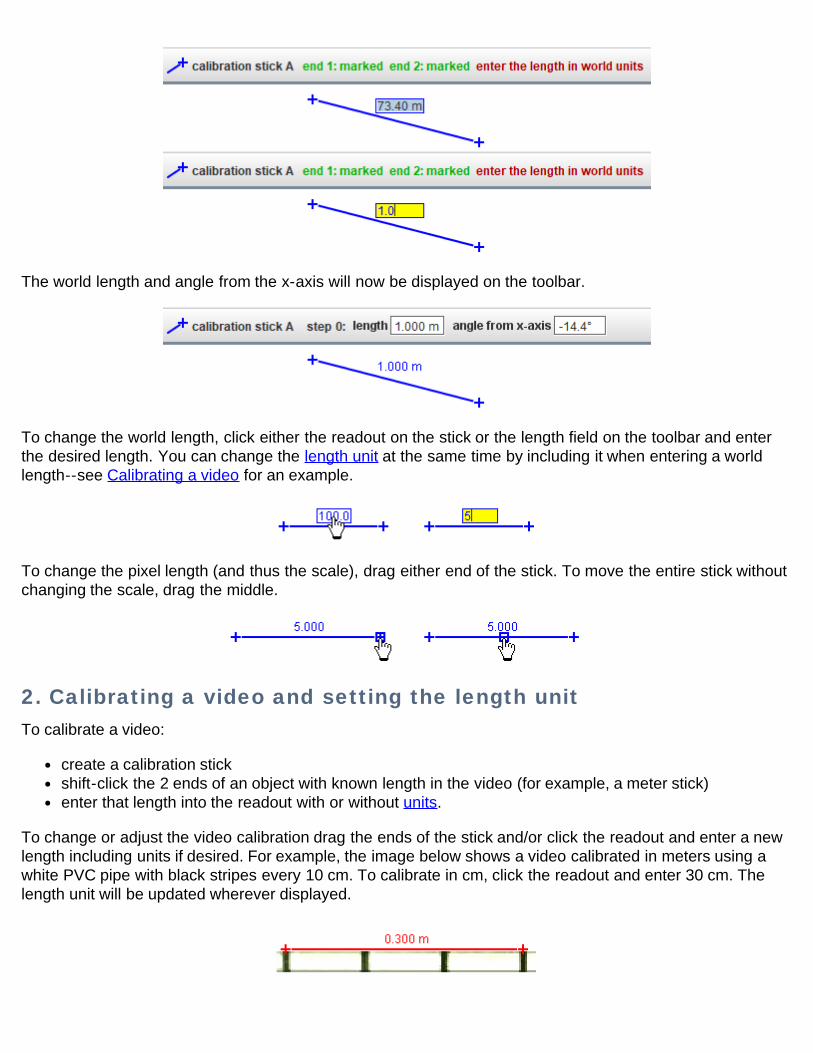
The world length and angle from the x-axis will now be displayed on the toolbar.

To change the world length, click either the readout on the stick or the length field on the toolbar and enterthe desired length. You can change the length unit at the same time by including it when entering a worldlength--see Calibrating a video for an example.

To change the pixel length (and thus the scale), drag either end of the stick. To move the entire stick withoutchanging the scale, drag the middle.

2. Calibrating a video and setting the length unitTo calibrate a video:

create a calibration stickshift-click the 2 ends of an object with known length in the video (for example, a meter stick)enter that length into the readout with or without units.

To change or adjust the video calibration drag the ends of the stick and/or click the readout and enter a newlength including units if desired. For example, the image below shows a video calibrated in meters using awhite PVC pipe with black stripes every 10 cm. To calibrate in cm, click the readout and enter 30 cm. Thelength unit will be updated wherever displayed.

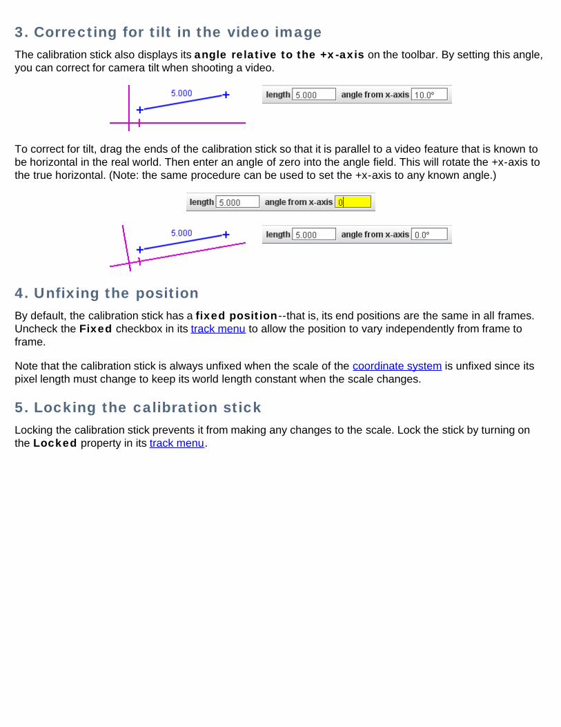
3. Correcting for tilt in the video imageThe calibration stick also displays its angle relative to the +x-axis on the toolbar. By setting this angle,you can correct for camera tilt when shooting a video.

To correct for tilt, drag the ends of the calibration stick so that it is parallel to a video feature that is known tobe horizontal in the real world. Then enter an angle of zero into the angle field. This will rotate the +x-axis tothe true horizontal. (Note: the same procedure can be used to set the +x-axis to any known angle.)

4. Unfixing the positionBy default, the calibration stick has a fixed position--that is, its end positions are the same in all frames.Uncheck the Fixed checkbox in its track menu to allow the position to vary independently from frame toframe.

Note that the calibration stick is always unfixed when the scale of the coordinate system is unfixed since itspixel length must change to keep its world length constant when the scale changes.

5. Locking the calibration stickLocking the calibration stick prevents it from making any changes to the scale. Lock the stick by turning onthe Locked property in its track menu.

Offset Origin

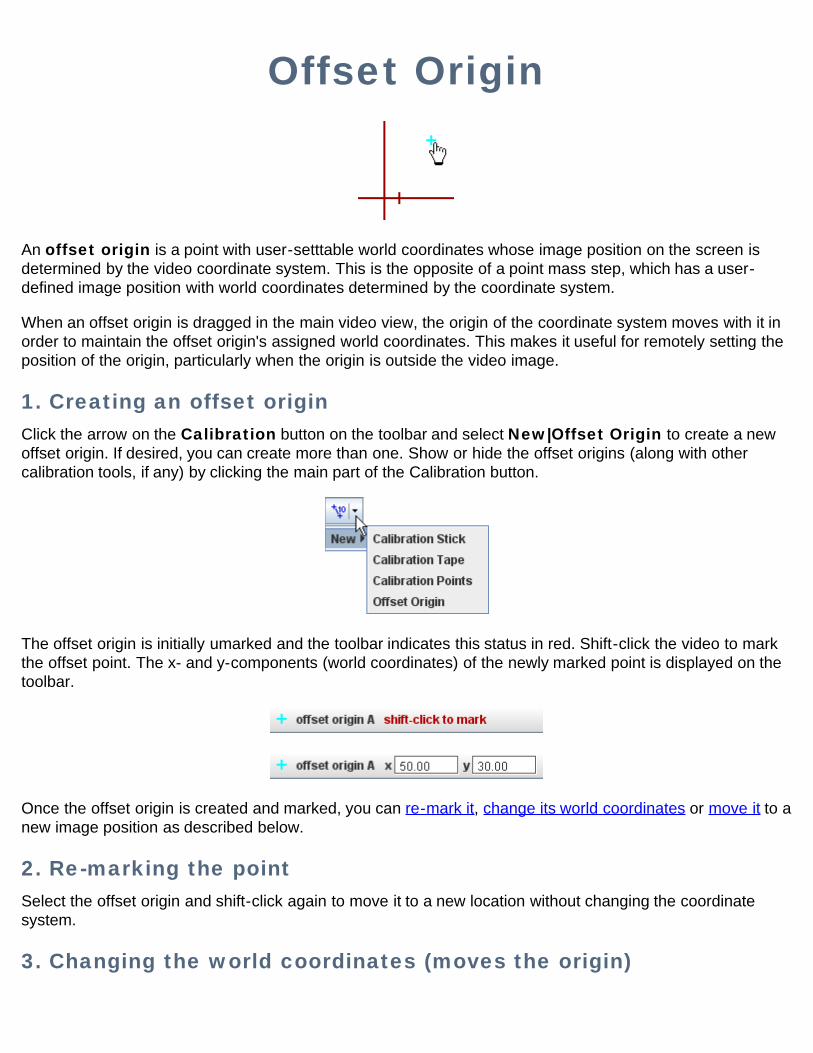
An offset origin is a point with user-setttable world coordinates whose image position on the screen isdetermined by the video coordinate system. This is the opposite of a point mass step, which has a user-defined image position with world coordinates determined by the coordinate system.

When an offset origin is dragged in the main video view, the origin of the coordinate system moves with it inorder to maintain the offset origin's assigned world coordinates. This makes it useful for remotely setting theposition of the origin, particularly when the origin is outside the video image.

1. Creating an offset originClick the arrow on the Calibration button on the toolbar and select New|Offset Origin to create a newoffset origin. If desired, you can create more than one. Show or hide the offset origins (along with othercalibration tools, if any) by clicking the main part of the Calibration button.

The offset origin is initially umarked and the toolbar indicates this status in red. Shift-click the video to markthe offset point. The x- and y-components (world coordinates) of the newly marked point is displayed on thetoolbar.

Once the offset origin is created and marked, you can re-mark it, change its world coordinates or move it to anew image position as described below.

2. Re-marking the pointSelect the offset origin and shift-click again to move it to a new location without changing the coordinatesystem.

3. Changing the world coordinates (moves the origin)

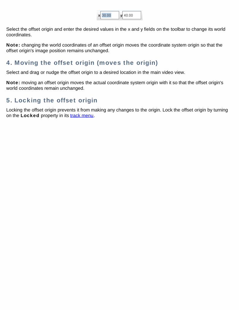
Select the offset origin and enter the desired values in the x and y fields on the toolbar to change its worldcoordinates.

Note: changing the world coordinates of an offset origin moves the coordinate system origin so that theoffset origin's image position remains unchanged.

4. Moving the offset origin (moves the origin)Select and drag or nudge the offset origin to a desired location in the main video view.

Note: moving an offset origin moves the actual coordinate system origin with it so that the offset origin'sworld coordinates remain unchanged.

5. Locking the offset originLocking the offset origin prevents it from making any changes to the origin. Lock the offset origin by turningon the Locked property in its track menu.

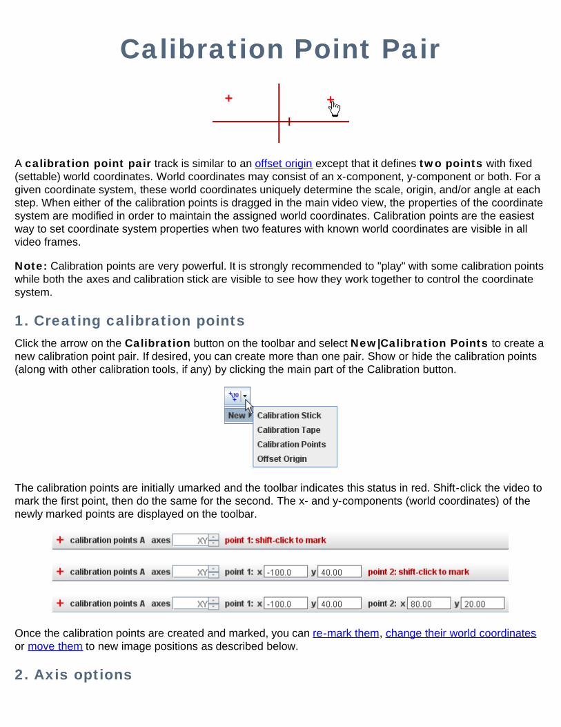
Calibration Point Pair

A calibration point pair track is similar to an offset origin except that it defines two points with fixed(settable) world coordinates. World coordinates may consist of an x-component, y-component or both. For agiven coordinate system, these world coordinates uniquely determine the scale, origin, and/or angle at eachstep. When either of the calibration points is dragged in the main video view, the properties of the coordinatesystem are modified in order to maintain the assigned world coordinates. Calibration points are the easiestway to set coordinate system properties when two features with known world coordinates are visible in allvideo frames.

Note: Calibration points are very powerful. It is strongly recommended to "play" with some calibration pointswhile both the axes and calibration stick are visible to see how they work together to control the coordinatesystem.

1. Creating calibration pointsClick the arrow on the Calibration button on the toolbar and select New|Calibration Points to create anew calibration point pair. If desired, you can create more than one pair. Show or hide the calibration points(along with other calibration tools, if any) by clicking the main part of the Calibration button.

The calibration points are initially umarked and the toolbar indicates this status in red. Shift-click the video tomark the first point, then do the same for the second. The x- and y-components (world coordinates) of thenewly marked points are displayed on the toolbar.

Once the calibration points are created and marked, you can re-mark them, change their world coordinatesor move them to new image positions as described below.

2. Axis options

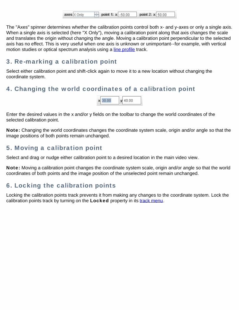
The "Axes" spinner determines whether the calibration points control both x- and y-axes or only a single axis.When a single axis is selected (here "X Only"), moving a calibration point along that axis changes the scaleand translates the origin without changing the angle. Moving a calibration point perpendicular to the selectedaxis has no effect. This is very useful when one axis is unknown or unimportant--for example, with verticalmotion studies or optical spectrum analysis using a line profile track.

3. Re-marking a calibration pointSelect either calibration point and shift-click again to move it to a new location without changing thecoordinate system.

4. Changing the world coordinates of a calibration point

Enter the desired values in the x and/or y fields on the toolbar to change the world coordinates of theselected calibration point.

Note: Changing the world coordinates changes the coordinate system scale, origin and/or angle so that theimage positions of both points remain unchanged.

5. Moving a calibration pointSelect and drag or nudge either calibration point to a desired location in the main video view.

Note: Moving a calibration point changes the coordinate system scale, origin and/or angle so that the worldcoordinates of both points and the image position of the unselected point remain unchanged.

6. Locking the calibration pointsLocking the calibration points track prevents it from making any changes to the coordinate system. Lock thecalibration points track by turning on the Locked property in its track menu.

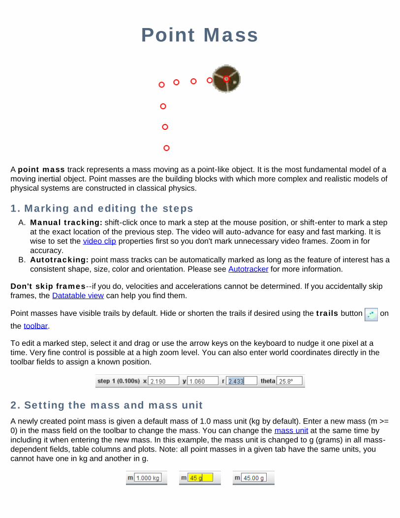
Point Mass

A point mass track represents a mass moving as a point-like object. It is the most fundamental model of amoving inertial object. Point masses are the building blocks with which more complex and realistic models ofphysical systems are constructed in classical physics.

1. Marking and editing the stepsA. Manual tracking: shift-click once to mark a step at the mouse position, or shift-enter to mark a step

at the exact location of the previous step. The video will auto-advance for easy and fast marking. It iswise to set the video clip properties first so you don't mark unnecessary video frames. Zoom in foraccuracy.

B. Autotracking: point mass tracks can be automatically marked as long as the feature of interest has aconsistent shape, size, color and orientation. Please see Autotracker for more information.

Don't skip frames--if you do, velocities and accelerations cannot be determined. If you accidentally skipframes, the Datatable view can help you find them.

Point masses have visible trails by default. Hide or shorten the trails if desired using the trails button onthe toolbar.

To edit a marked step, select it and drag or use the arrow keys on the keyboard to nudge it one pixel at atime. Very fine control is possible at a high zoom level. You can also enter world coordinates directly in thetoolbar fields to assign a known position.

2. Setting the mass and mass unitA newly created point mass is given a default mass of 1.0 mass unit (kg by default). Enter a new mass (m >=0) in the mass field on the toolbar to change the mass. You can change the mass unit at the same time byincluding it when entering the new mass. In this example, the mass unit is changed to g (grams) in all mass-dependent fields, table columns and plots. Note: all point masses in a given tab have the same units, youcannot have one in kg and another in g.

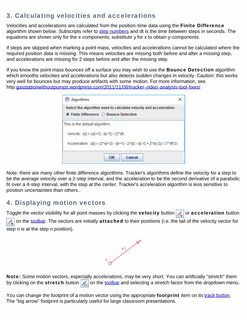
3. Calculating velocities and accelerationsVelocities and accelerations are calculated from the position-time data using the Finite Differencealgorithm shown below. Subscripts refer to step numbers and dt is the time between steps in seconds. Theequations are shown only for the x-components; substitute y for x to obtain y-components.

If steps are skipped when marking a point mass, velocities and accelerations cannot be calculated where therequired position data is missing. This means velocities are missing both before and after a missing step,and accelerations are missing for 2 steps before and after the missing step.

If you know the point mass bounces off a surface you may wish to use the Bounce Detection algorithmwhich smooths velocities and accelerations but also detects sudden changes in velocity. Caution: this worksvery well for bounces but may produce artifacts with some motion. For more information, seehttp:gasstationwithoutpumps.wordpress.com/2011/11/08/tracker-video-analysis-tool-fixes/

Note: there are many other finite difference algorithms. Tracker's algorithms define the velocity for a step tobe the average velocity over a 2-step interval, and the acceleration to be the second derivative of a parabolicfit over a 4-step interval, with the step at the center. Tracker's acceleration algorithm is less sensitive toposition uncertainties than others..

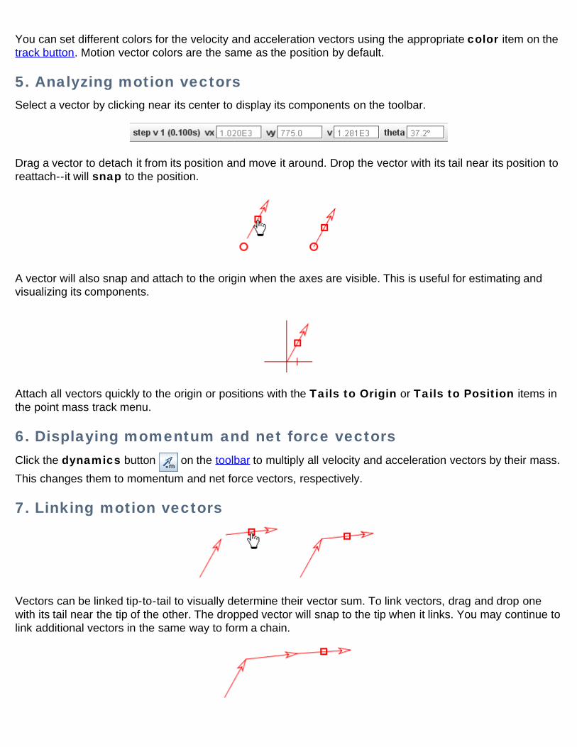
4. Displaying motion vectorsToggle the vector visibility for all point masses by clicking the velocity button or acceleration button

on the toolbar. The vectors are initially attached to their positions (i.e. the tail of the velocity vector forstep n is at the step n position).

Note: Some motion vectors, especially accelerations, may be very short. You can artificially "stretch" themby clicking on the stretch button on the toolbar and selecting a stretch factor from the dropdown menu.

You can change the footprint of a motion vector using the appropriate footprint item on its track button.The ”big arrow” footprint is particularly useful for large classroom presentations.

You can set different colors for the velocity and acceleration vectors using the appropriate color item on thetrack button. Motion vector colors are the same as the position by default.

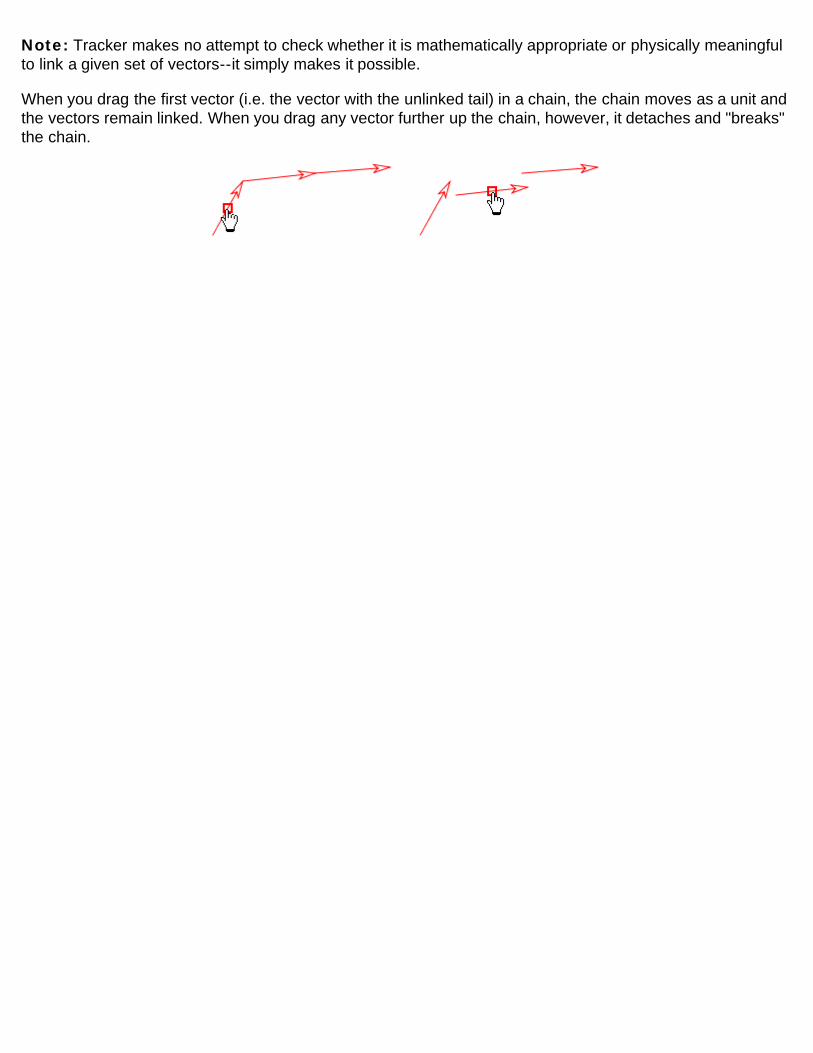
5. Analyzing motion vectorsSelect a vector by clicking near its center to display its components on the toolbar.

Drag a vector to detach it from its position and move it around. Drop the vector with its tail near its position toreattach--it will snap to the position.

A vector will also snap and attach to the origin when the axes are visible. This is useful for estimating andvisualizing its components.

Attach all vectors quickly to the origin or positions with the Tails to Origin or Tails to Position items inthe point mass track menu.

6. Displaying momentum and net force vectorsClick the dynamics button on the toolbar to multiply all velocity and acceleration vectors by their mass.This changes them to momentum and net force vectors, respectively.

7. Linking motion vectors

Vectors can be linked tip-to-tail to visually determine their vector sum. To link vectors, drag and drop onewith its tail near the tip of the other. The dropped vector will snap to the tip when it links. You may continue tolink additional vectors in the same way to form a chain.

Note: Tracker makes no attempt to check whether it is mathematically appropriate or physically meaningfulto link a given set of vectors--it simply makes it possible.

When you drag the first vector (i.e. the vector with the unlinked tail) in a chain, the chain moves as a unit andthe vectors remain linked. When you drag any vector further up the chain, however, it detaches and "breaks"the chain.

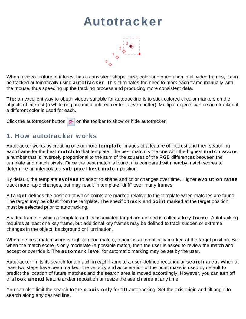
Autotracker

When a video feature of interest has a consistent shape, size, color and orientation in all video frames, it canbe tracked automatically using autotracker. This eliminates the need to mark each frame manually withthe mouse, thus speeding up the tracking process and producing more consistent data.

Tip: an excellent way to obtain videos suitable for autotracking is to stick colored circular markers on theobjects of interest (a white ring around a colored center is even better). Multiple objects can be autotracked ifa different color is used for each.

Click the autotracker button on the toolbar to show or hide autotracker.

1. How autotracker worksAutotracker works by creating one or more template images of a feature of interest and then searchingeach frame for the best match to that template. The best match is the one with the highest match score,a number that is inversely proportional to the sum of the squares of the RGB differences between thetemplate and match pixels. Once the best match is found, it is compared with nearby match scores todetermine an interpolated sub-pixel best match position.

By default, the template evolves to adapt to shape and color changes over time. Higher evolution ratestrack more rapid changes, but may result in template "drift" over many frames.

A target defines the position at which points are marked relative to the template when matches are found.The target may be offset from the template. The specific track and point marked at the target positionmust be selected prior to autotracking.

A video frame in which a template and its associated target are defined is called a key frame. Autotrackingrequires at least one key frame, but additional key frames may be defined to track sudden or extremechanges in the object, background or illumination.

When the best match score is high (a good match), a point is automatically marked at the target position. Butwhen the match score is only moderate (a possible match) then the user is asked to review the match andaccept or override it. The automark level for automatic marking may be set by the user.

Autotracker limits its search for a match in each frame to a user-defined rectangular search area. When atleast two steps have been marked, the velocity and acceleration of the point mass is used by default topredict the location of future matches and the search area is moved accordingly. However, you can turn offthis look ahead feature and/or reposition or resize the search area at any time.

You can also limit the search to the x-axis only for 1D autotracking. Set the axis origin and tilt angle tosearch along any desired line.

A specialized option is to search all frames non-stop using a fixed area and fixed template. For moreinformation see Other buttons in the Setting and controls section below.

After autotracker has completed the marking process, you may modify the steps at will. In other words,autotracker helps you mark the steps but does not limit your control over them.

2. Preparing to use autotrackerBefore using autotracker, scan through the video and verify that the feature of interest is visible andreasonably consistent (shape, size, color and orientation) in all frames. If not, adjust the video clip startframe, end frame and/or step size until this condition is met. Then reset the video to the start frame.

If planning to autotrack a very long video, it is useful to turn off auto-refresh in order to speed up the markingprocess. To turn off auto-refresh, click the Refresh button on the toolbar and uncheck the Auto-refreshitem in the popup menu. When done marking, turn auto-refresh back on or refresh the data manually bychoosing the Refresh item in the popup menu.

3. Using autotracker1. Select the target track.2. Shift-control-click the video feature of interest to create a key frame. This will display autotracker if it is

not already visible.3. Change the default settings if desired.4. Click the Search button.

Figure 1 shows autotracker after creating a key frame. The template is outlined on the video and shown at 2xmagnification in autotracker along with the (perfect) match found. The target point is indicated by a boldcross on the video and the search area is outlined with a dashed line.

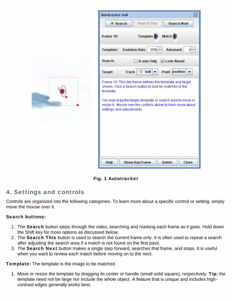
Fig. 1 Autotracker

4. Settings and controlsControls are organized into the following categories. To learn more about a specific control or setting, simplymove the mouse over it.

Search buttons:

1. The Search button steps through the video, searching and marking each frame as it goes. Hold downthe Shift key for more options as discussed below.

2. The Search This button is used to search the current frame only. It is often used to repeat a searchafter adjusting the search area if a match is not found on the first pass.

3. The Search Next button makes a single step forward, searches that frame, and stops. It is usefulwhen you want to review each match before moving on to the next.

Template: The template is the image to be matched.

1. Move or resize the template by dragging its center or handle (small solid square), respectively. Tip: thetemplate need not be large nor include the whole object. A feature that is unique and includes high-contrast edges generally works best.

2. Set the evolution rate to define how the template adapts to shape and color changes. An evolutionrate of 0% does not evolve at all (constant template image) while an evolution rate of 100% completelyreplaces the template with the match image after each frame. Intermediate evolution rates overlay thematch image onto the current template with the indicated opacity. Note: higher evolution rates trackmore rapid changes, but may result in template "drift" over many frames.

3. Set the automark level to define the minimum match score needed for automatic marking. Thedefault level of 4 is recommended as a good starting point. Tip: low automark levels can result in falsematches--try increasing the evolution rate or defining additional key frames instead.

Search: The search area defines the region that is searched for the best match.

1. Move or resize the search area by dragging its center or handle (small solid square), respectively. Tip:The search area need not be large. For many motions the look-ahead feature does a good job ofpredicting match positions and searching in the right place.

2. Check the X-axis Only checkbox to limit the search to the x-axis only. The coordinate system originwill automatically be set to the center of the template. Tilt the axes to search in the desired direction.Note: if the x-axis does not pass through or near the center of the search area, no matches will befound.

3. Check the Look Ahead checkbox to automatically move the search area to predicted matchpositions using a look-ahead algorithm that assumes constant acceleration. When this option isunchecked, the search area is moved to the previous match position.

Target: The target defines both the track and point to be marked and the position of the mark relative to thetemplate.

1. Select the target track and point from the drop-down lists.2. Move the target by dragging it.

Other buttons:

1. The Help button shows this help file.2. The Show Key Frame button enables you to quickly jump to a key frame to review and/or change

the template or target.3. The Delete button enables you to easily delete incorrectly marked points.4. The Close button closes autotracker.5. The Options button (Shift-Search button) pops up a menu with the following items:

Search Fixed Area: searches for matches in all frames using the current (fixed) template andsearch area. This steps through all frames non-stop no matter what match scores are found. Anexample of how this can be useful is determining the motion of a moving (translating) camera. If acalibration tape with regularly spaced black dots is included in the background, and a (small) fixedarea search is made using a black dot template, then a good match will be found every time ablack dot enters the area. The resulting match data can be used to determine the camera speed.Copy Match Data: copies match data (frame numbers, non-null match scores and positions)to the clipboard for pasting into a spreadsheet or other document. (Note: match data cannot bedisplayed in Tracker data tables because they are generated by templates, not by tracks.)

5. Search resultsAfter searching a frame, autotracker will display one of the following search results and, in some cases,present options for solving problems.

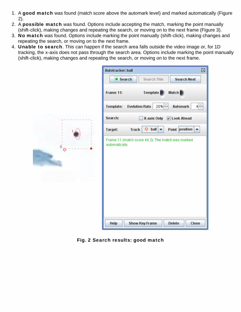
1. A good match was found (match score above the automark level) and marked automatically (Figure2).

2. A possible match was found. Options include accepting the match, marking the point manually(shift-click), making changes and repeating the search, or moving on to the next frame (Figure 3).

3. No match was found. Options include marking the point manually (shift-click), making changes andrepeating the search, or moving on to the next frame.

4. Unable to search. This can happen if the search area falls outside the video image or, for 1Dtracking, the x-axis does not pass through the search area. Options include marking the point manually(shift-click), making changes and repeating the search, or moving on to the next frame.

Fig. 2 Search results: good match

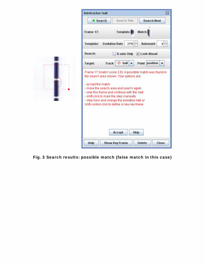
Fig. 3 Search results: possible match (false match in this case)

Center of Mass

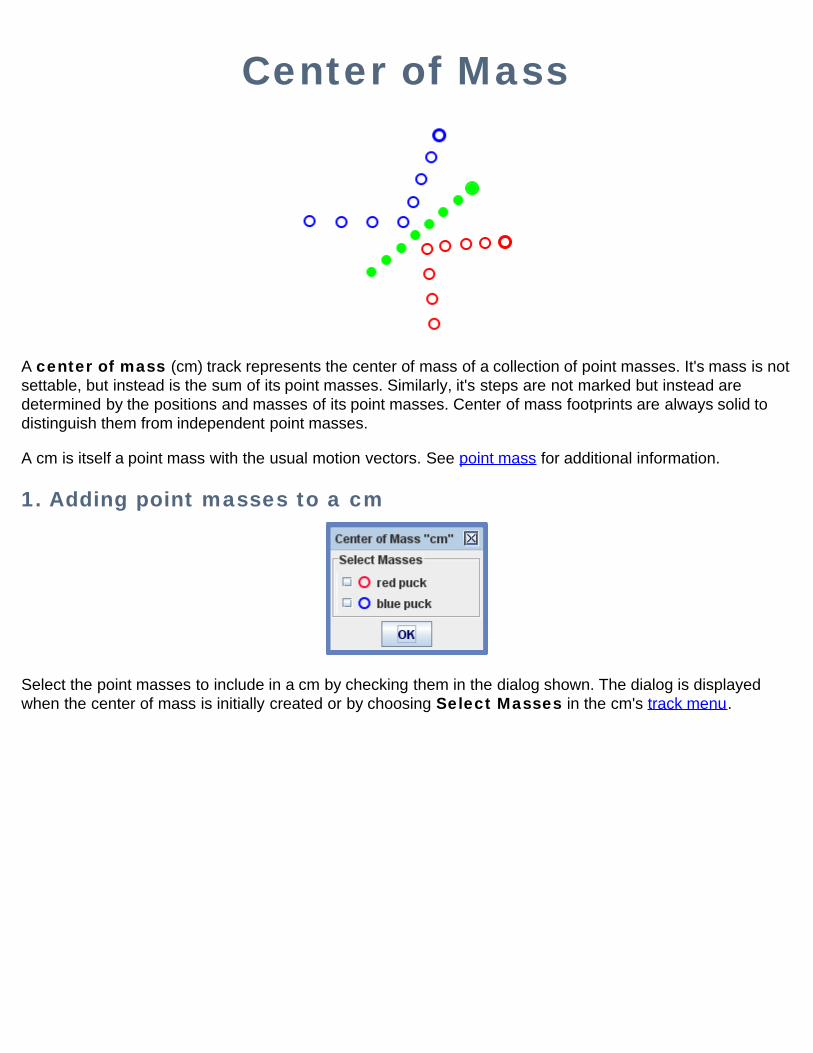
A center of mass (cm) track represents the center of mass of a collection of point masses. It's mass is notsettable, but instead is the sum of its point masses. Similarly, it's steps are not marked but instead aredetermined by the positions and masses of its point masses. Center of mass footprints are always solid todistinguish them from independent point masses.

A cm is itself a point mass with the usual motion vectors. See point mass for additional information.

1. Adding point masses to a cm

Select the point masses to include in a cm by checking them in the dialog shown. The dialog is displayedwhen the center of mass is initially created or by choosing Select Masses in the cm's track menu.

Vector

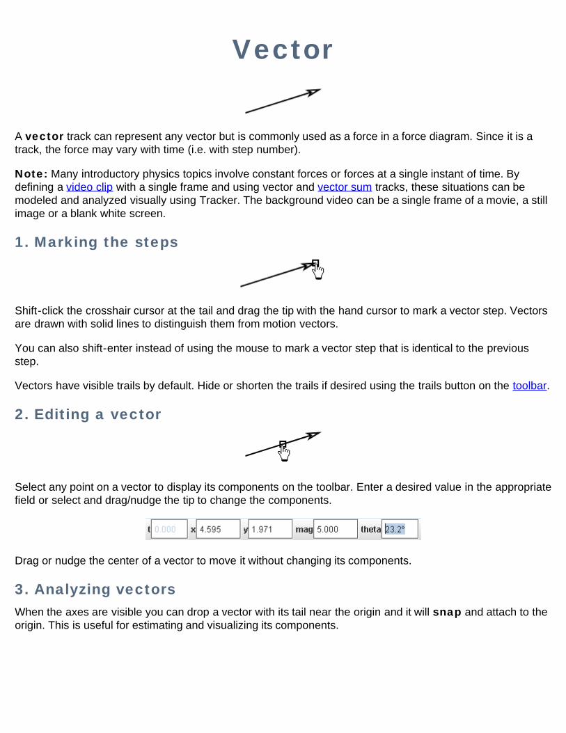
A vector track can represent any vector but is commonly used as a force in a force diagram. Since it is atrack, the force may vary with time (i.e. with step number).

Note: Many introductory physics topics involve constant forces or forces at a single instant of time. Bydefining a video clip with a single frame and using vector and vector sum tracks, these situations can bemodeled and analyzed visually using Tracker. The background video can be a single frame of a movie, a stillimage or a blank white screen.

1. Marking the steps

Shift-click the crosshair cursor at the tail and drag the tip with the hand cursor to mark a vector step. Vectorsare drawn with solid lines to distinguish them from motion vectors.

You can also shift-enter instead of using the mouse to mark a vector step that is identical to the previousstep.

Vectors have visible trails by default. Hide or shorten the trails if desired using the trails button on the toolbar.

2. Editing a vector

Select any point on a vector to display its components on the toolbar. Enter a desired value in the appropriatefield or select and drag/nudge the tip to change the components.

Drag or nudge the center of a vector to move it without changing its components.

3. Analyzing vectorsWhen the axes are visible you can drop a vector with its tail near the origin and it will snap and attach to theorigin. This is useful for estimating and visualizing its components.

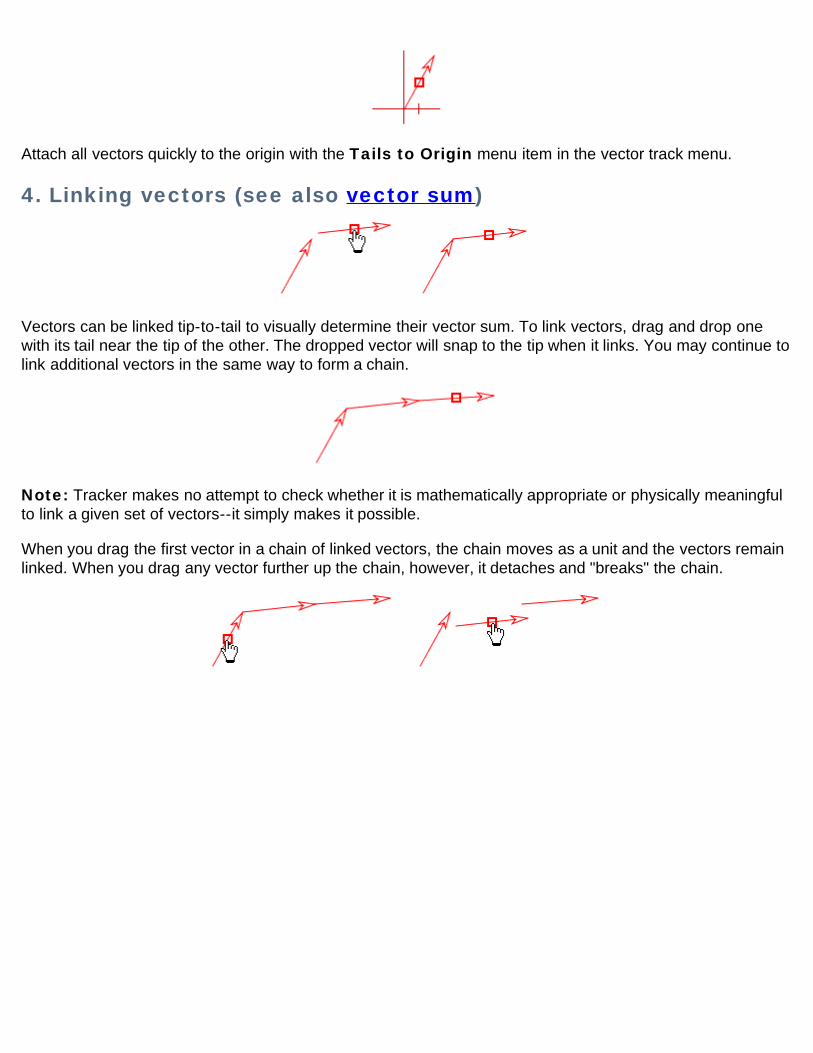
Attach all vectors quickly to the origin with the Tails to Origin menu item in the vector track menu.

4. Linking vectors (see also vector sum)

Vectors can be linked tip-to-tail to visually determine their vector sum. To link vectors, drag and drop onewith its tail near the tip of the other. The dropped vector will snap to the tip when it links. You may continue tolink additional vectors in the same way to form a chain.

Note: Tracker makes no attempt to check whether it is mathematically appropriate or physically meaningfulto link a given set of vectors--it simply makes it possible.

When you drag the first vector in a chain of linked vectors, the chain moves as a unit and the vectors remainlinked. When you drag any vector further up the chain, however, it detaches and "breaks" the chain.

Vector Sum

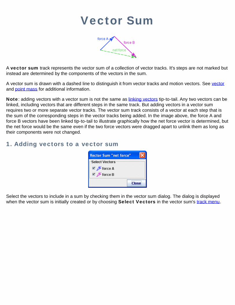
A vector sum track represents the vector sum of a collection of vector tracks. It's steps are not marked butinstead are determined by the components of the vectors in the sum.

A vector sum is drawn with a dashed line to distinguish it from vector tracks and motion vectors. See vectorand point mass for additional information.

Note: adding vectors with a vector sum is not the same as linking vectors tip-to-tail. Any two vectors can belinked, including vectors that are different steps in the same track. But adding vectors in a vector sumrequires two or more separate vector tracks. The vector sum track consists of a vector at each step that isthe sum of the corresponding steps in the vector tracks being added. In the image above, the force A andforce B vectors have been linked tip-to-tail to illustrate graphically how the net force vector is determined, butthe net force would be the same even if the two force vectors were dragged apart to unlink them as long astheir components were not changed.

1. Adding vectors to a vector sum

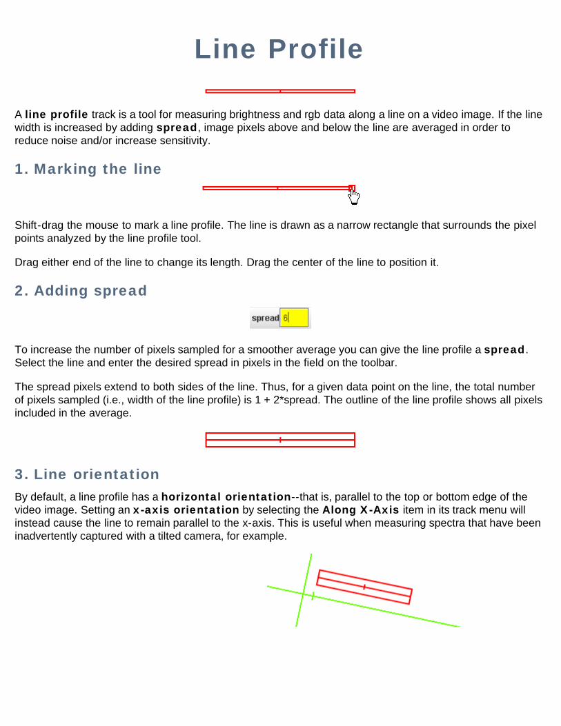
Select the vectors to include in a sum by checking them in the vector sum dialog. The dialog is displayedwhen the vector sum is initially created or by choosing Select Vectors in the vector sum's track menu.

Line Profile

A line profile track is a tool for measuring brightness and rgb data along a line on a video image. If the linewidth is increased by adding spread, image pixels above and below the line are averaged in order toreduce noise and/or increase sensitivity.

1. Marking the line

Shift-drag the mouse to mark a line profile. The line is drawn as a narrow rectangle that surrounds the pixelpoints analyzed by the line profile tool.

Drag either end of the line to change its length. Drag the center of the line to position it.

2. Adding spread

To increase the number of pixels sampled for a smoother average you can give the line profile a spread.Select the line and enter the desired spread in pixels in the field on the toolbar.

The spread pixels extend to both sides of the line. Thus, for a given data point on the line, the total numberof pixels sampled (i.e., width of the line profile) is 1 + 2*spread. The outline of the line profile shows all pixelsincluded in the average.

3. Line orientationBy default, a line profile has a horizontal orientation--that is, parallel to the top or bottom edge of thevideo image. Setting an x-axis orientation by selecting the Along X-Axis item in its track menu willinstead cause the line to remain parallel to the x-axis. This is useful when measuring spectra that have beeninadvertently captured with a tilted camera, for example.

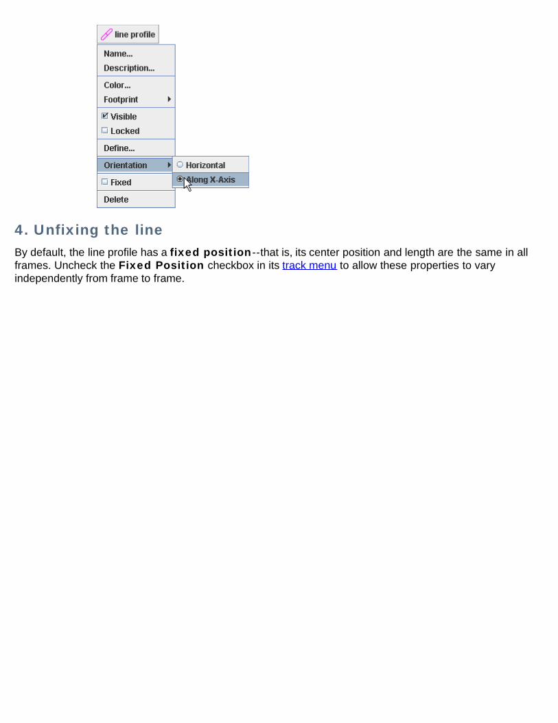
4. Unfixing the lineBy default, the line profile has a fixed position--that is, its center position and length are the same in allframes. Uncheck the Fixed Position checkbox in its track menu to allow these properties to varyindependently from frame to frame.

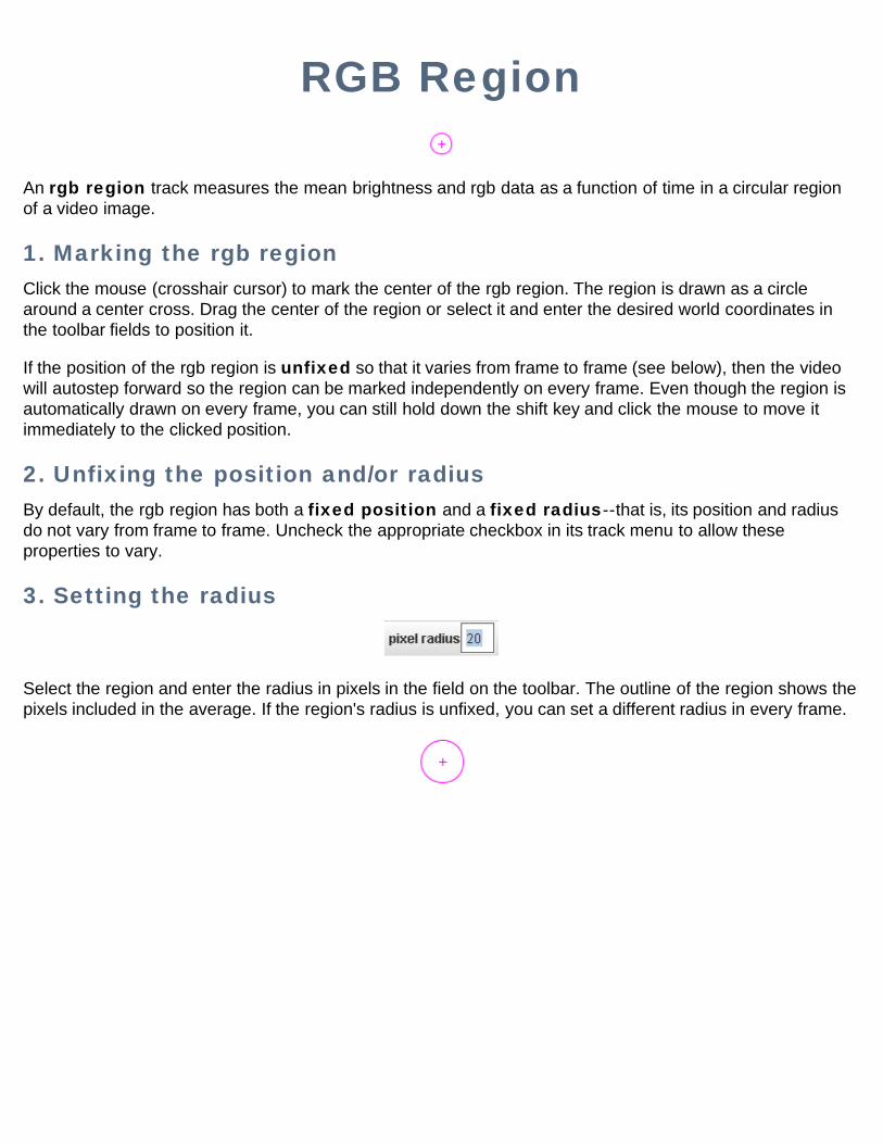
RGB Region

An rgb region track measures the mean brightness and rgb data as a function of time in a circular regionof a video image.

1. Marking the rgb regionClick the mouse (crosshair cursor) to mark the center of the rgb region. The region is drawn as a circlearound a center cross. Drag the center of the region or select it and enter the desired world coordinates inthe toolbar fields to position it.

If the position of the rgb region is unfixed so that it varies from frame to frame (see below), then the videowill autostep forward so the region can be marked independently on every frame. Even though the region isautomatically drawn on every frame, you can still hold down the shift key and click the mouse to move itimmediately to the clicked position.

2. Unfixing the position and/or radiusBy default, the rgb region has both a fixed position and a fixed radius--that is, its position and radiusdo not vary from frame to frame. Uncheck the appropriate checkbox in its track menu to allow theseproperties to vary.

3. Setting the radius

Select the region and enter the radius in pixels in the field on the toolbar. The outline of the region shows thepixels included in the average. If the region's radius is unfixed, you can set a different radius in every frame.

Particle Models

A particle model track is a mathematical model of a point mass. The step positions of the particle are determined by theparameters of the model rather than being marked with the mouse.

There are two types of particle models: kinematic and dynamic. A kinematic particle defines position functions of time(Figure 4), while a dynamic particle defines force functions and initial conditions for numerical ODE solvers (Figure 1). Dynamicparticles may be defined in either cartesian or polar coordinates.

Model particles have a start and end frame that define the frames of the video in which they are drawn. This makes itpossible to define multiple models that apply at different times in the same video.

A dynamic particle may use a launcher (point mass) to set its initial position and velocity. Launchers can be quite powerful--for more information, see Launching dynamic particles.

A particle model has a settable mass and generates motion data and vectors just like any other point mass. See point mass foradditional information.

A particle model can create a stamped point mass which clones the model's current positions. The stamped point masspositions don't move when you change scale. For more information see Stamping a point mass.

1. Building particle modelsParticle model properties are displayed and edited using the Model Builder tool. To use the builder, choose Model Builder...from the model's track menu.

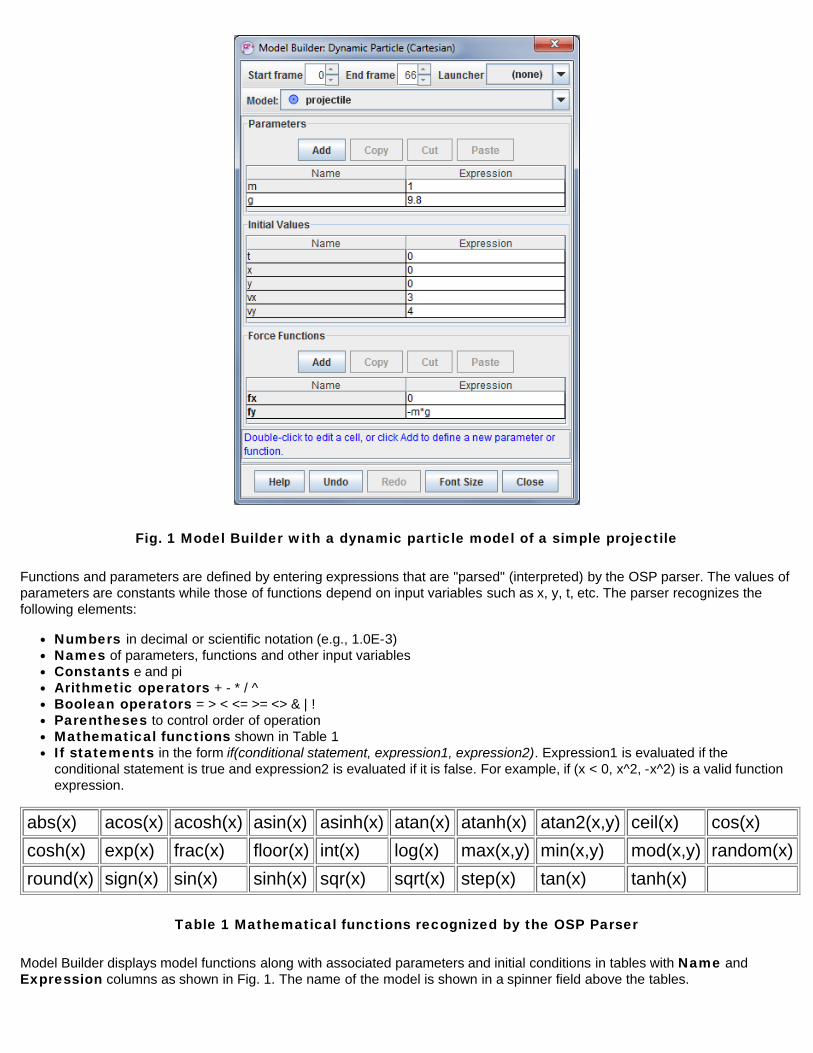
Fig. 1 Model Builder with a dynamic particle model of a simple projectile

Functions and parameters are defined by entering expressions that are "parsed" (interpreted) by the OSP parser. The values ofparameters are constants while those of functions depend on input variables such as x, y, t, etc. The parser recognizes thefollowing elements:

Numbers in decimal or scientific notation (e.g., 1.0E-3)Names of parameters, functions and other input variablesConstants e and piArithmetic operators + - * / ^Boolean operators = > < <= >= <> & | !Parentheses to control order of operationMathematical functions shown in Table 1If statements in the form if(conditional statement, expression1, expression2). Expression1 is evaluated if theconditional statement is true and expression2 is evaluated if it is false. For example, if (x < 0, x^2, -x^2) is a valid functionexpression.

abs(x) acos(x) acosh(x) asin(x) asinh(x) atan(x) atanh(x) atan2(x,y) ceil(x) cos(x)cosh(x) exp(x) frac(x) floor(x) int(x) log(x) max(x,y) min(x,y) mod(x,y) random(x)round(x) sign(x) sin(x) sinh(x) sqr(x) sqrt(x) step(x) tan(x) tanh(x)

Table 1 Mathematical functions recognized by the OSP Parser

Model Builder displays model functions along with associated parameters and initial conditions in tables with Name andExpression columns as shown in Fig. 1. The name of the model is shown in a spinner field above the tables.

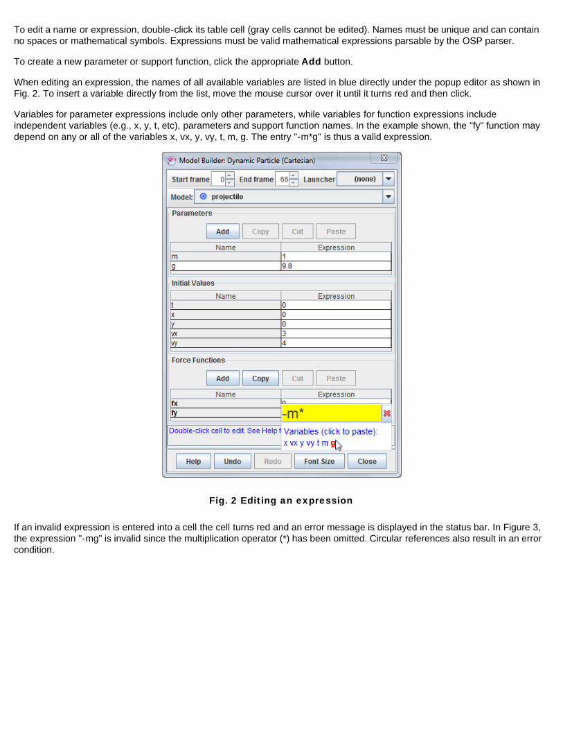
To edit a name or expression, double-click its table cell (gray cells cannot be edited). Names must be unique and can containno spaces or mathematical symbols. Expressions must be valid mathematical expressions parsable by the OSP parser.

To create a new parameter or support function, click the appropriate Add button.

When editing an expression, the names of all available variables are listed in blue directly under the popup editor as shown inFig. 2. To insert a variable directly from the list, move the mouse cursor over it until it turns red and then click.

Variables for parameter expressions include only other parameters, while variables for function expressions includeindependent variables (e.g., x, y, t, etc), parameters and support function names. In the example shown, the "fy" function maydepend on any or all of the variables x, vx, y, vy, t, m, g. The entry "-m*g" is thus a valid expression.

Fig. 2 Editing an expression

If an invalid expression is entered into a cell the cell turns red and an error message is displayed in the status bar. In Figure 3,the expression "-mg" is invalid since the multiplication operator (*) has been omitted. Circular references also result in an errorcondition.

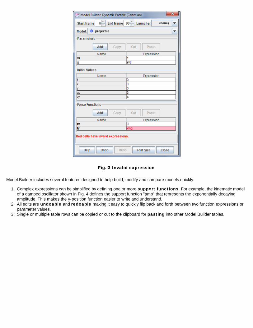
Fig. 3 Invalid expression

Model Builder includes several features designed to help build, modify and compare models quickly:

1. Complex expressions can be simplified by defining one or more support functions. For example, the kinematic modelof a damped oscillator shown in Fig. 4 defines the support function "amp" that represents the exponentially decayingamplitude. This makes the y-position function easier to write and understand.

2. All edits are undoable and redoable making it easy to quickly flip back and forth between two function expressions orparameter values.

3. Single or multiple table rows can be copied or cut to the clipboard for pasting into other Model Builder tables.

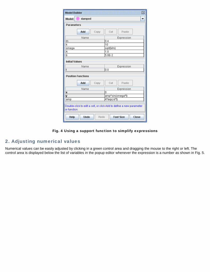
Fig. 4 Using a support function to simplify expressions

2. Adjusting numerical valuesNumerical values can be easily adjusted by clicking in a green control area and dragging the mouse to the right or left. Thecontrol area is displayed below the list of variables in the popup editor whenever the expression is a number as shown in Fig. 5.

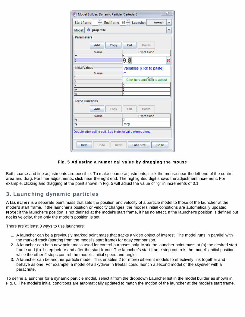
Fig. 5 Adjusting a numerical value by dragging the mouse

Both coarse and fine adjustments are possible. To make coarse adjustments, click the mouse near the left end of the controlarea and drag. For finer adjustments, click near the right end. The highlighted digit shows the adjustment increment. Forexample, clicking and dragging at the point shown in Fig. 5 will adjust the value of "g" in increments of 0.1.

3. Launching dynamic particlesA launcher is a separate point mass that sets the position and velocity of a particle model to those of the launcher at themodel's start frame. If the launcher's position or velocity changes, the model's initial conditions are automatically updated.Note: if the launcher's position is not defined at the model's start frame, it has no effect. If the launcher's position is defined butnot its velocity, then only the model's position is set.

There are at least 3 ways to use launchers:

1. A launcher can be a previously marked point mass that tracks a video object of interest. The model runs in parallel withthe marked track (starting from the model's start frame) for easy comparison.

2. A launcher can be a new point mass used for control purposes only. Mark the launcher point mass at (a) the desired startframe and (b) 1 step before and after the start frame. The launcher's start frame step controls the model's initial positionwhile the other 2 steps control the model's initial speed and angle.

3. A launcher can be another particle model. This enables 2 (or more) different models to effectively link together andbehave as one. For example, a model of a skydiver in freefall could launch a second model of the skydiver with aparachute.

To define a launcher for a dynamic particle model, select it from the dropdown Launcher list in the model builder as shown inFig. 6. The model's initial conditions are automatically updated to match the motion of the launcher at the model's start frame.

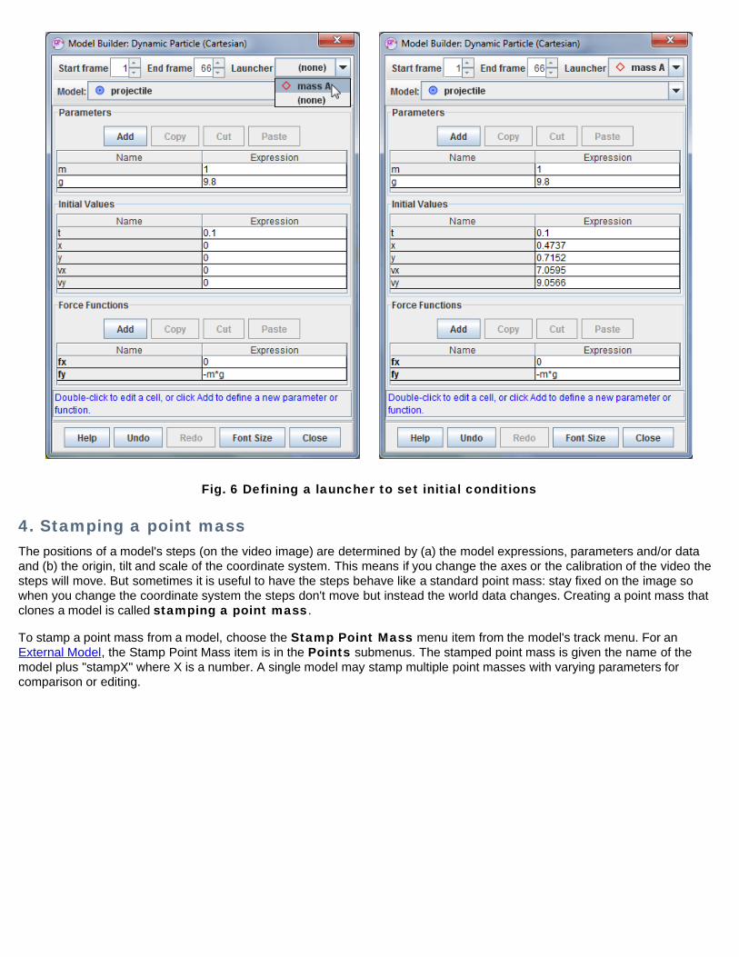
Fig. 6 Defining a launcher to set initial conditions

4. Stamping a point massThe positions of a model's steps (on the video image) are determined by (a) the model expressions, parameters and/or dataand (b) the origin, tilt and scale of the coordinate system. This means if you change the axes or the calibration of the video thesteps will move. But sometimes it is useful to have the steps behave like a standard point mass: stay fixed on the image sowhen you change the coordinate system the steps don't move but instead the world data changes. Creating a point mass thatclones a model is called stamping a point mass.

To stamp a point mass from a model, choose the Stamp Point Mass menu item from the model's track menu. For anExternal Model, the Stamp Point Mass item is in the Points submenus. The stamped point mass is given the name of themodel plus "stampX" where X is a number. A single model may stamp multiple point masses with varying parameters forcomparison or editing.

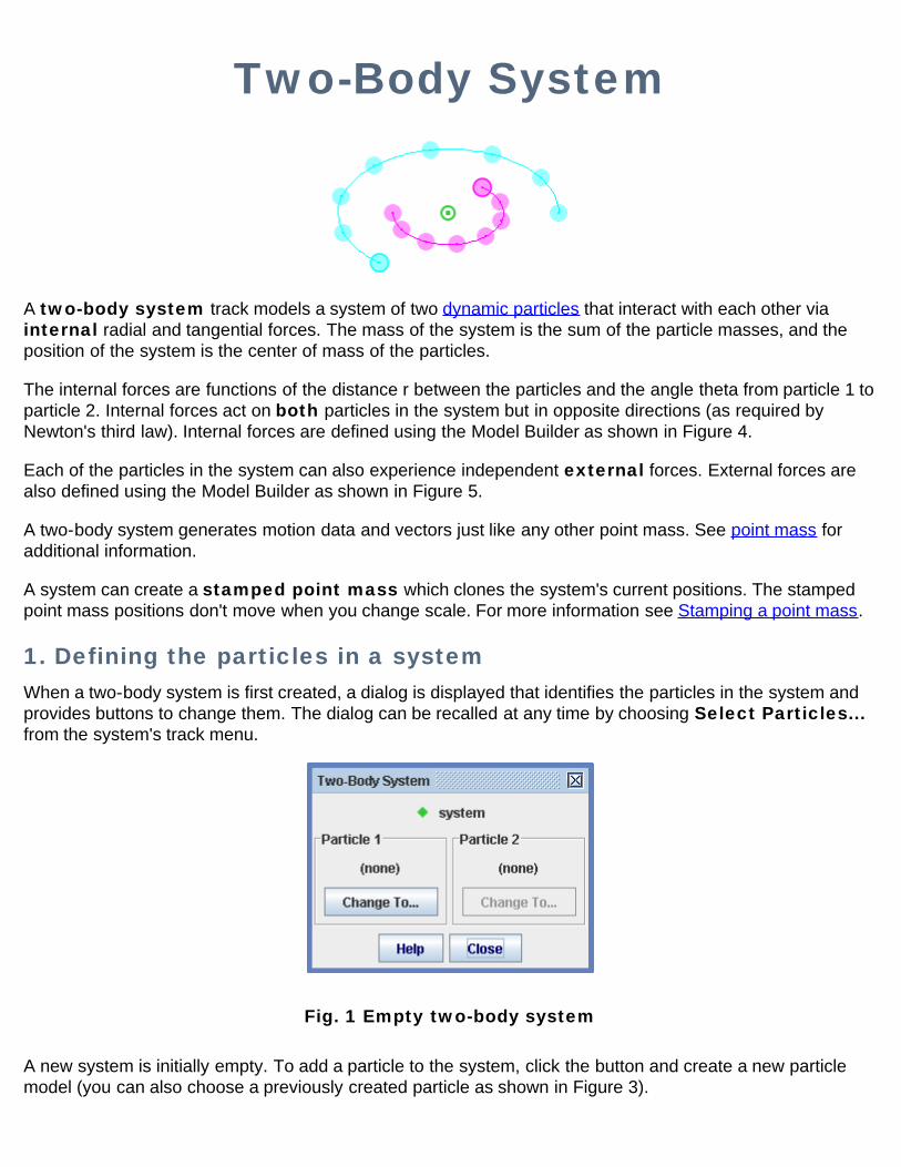
Two-Body System

A two-body system track models a system of two dynamic particles that interact with each other viainternal radial and tangential forces. The mass of the system is the sum of the particle masses, and theposition of the system is the center of mass of the particles.

The internal forces are functions of the distance r between the particles and the angle theta from particle 1 toparticle 2. Internal forces act on both particles in the system but in opposite directions (as required byNewton's third law). Internal forces are defined using the Model Builder as shown in Figure 4.

Each of the particles in the system can also experience independent external forces. External forces arealso defined using the Model Builder as shown in Figure 5.

A two-body system generates motion data and vectors just like any other point mass. See point mass foradditional information.

A system can create a stamped point mass which clones the system's current positions. The stampedpoint mass positions don't move when you change scale. For more information see Stamping a point mass.

1. Defining the particles in a systemWhen a two-body system is first created, a dialog is displayed that identifies the particles in the system andprovides buttons to change them. The dialog can be recalled at any time by choosing Select Particles...from the system's track menu.

Fig. 1 Empty two-body system

A new system is initially empty. To add a particle to the system, click the button and create a new particlemodel (you can also choose a previously created particle as shown in Figure 3).

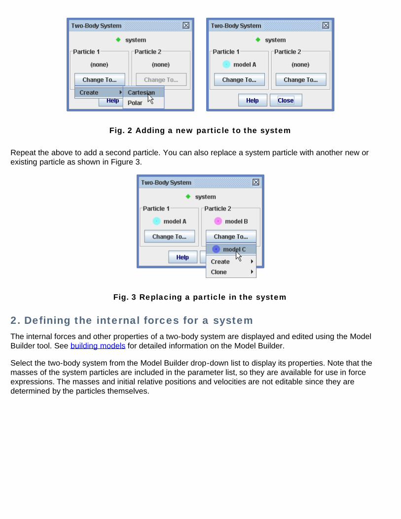
Fig. 2 Adding a new particle to the system

Repeat the above to add a second particle. You can also replace a system particle with another new orexisting particle as shown in Figure 3.

Fig. 3 Replacing a particle in the system

2. Defining the internal forces for a systemThe internal forces and other properties of a two-body system are displayed and edited using the ModelBuilder tool. See building models for detailed information on the Model Builder.

Select the two-body system from the Model Builder drop-down list to display its properties. Note that themasses of the system particles are included in the parameter list, so they are available for use in forceexpressions. The masses and initial relative positions and velocities are not editable since they aredetermined by the particles themselves.

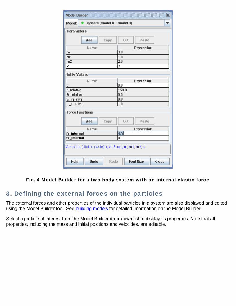
Fig. 4 Model Builder for a two-body system with an internal elastic force

3. Defining the external forces on the particlesThe external forces and other properties of the individual particles in a system are also displayed and editedusing the Model Builder tool. See building models for detailed information on the Model Builder.

Select a particle of interest from the Model Builder drop-down list to display its properties. Note that allproperties, including the mass and initial positions and velocities, are editable.

Fig. 5 Model Builder showing a particle model with non-zero initial position and velocitybut no external forces

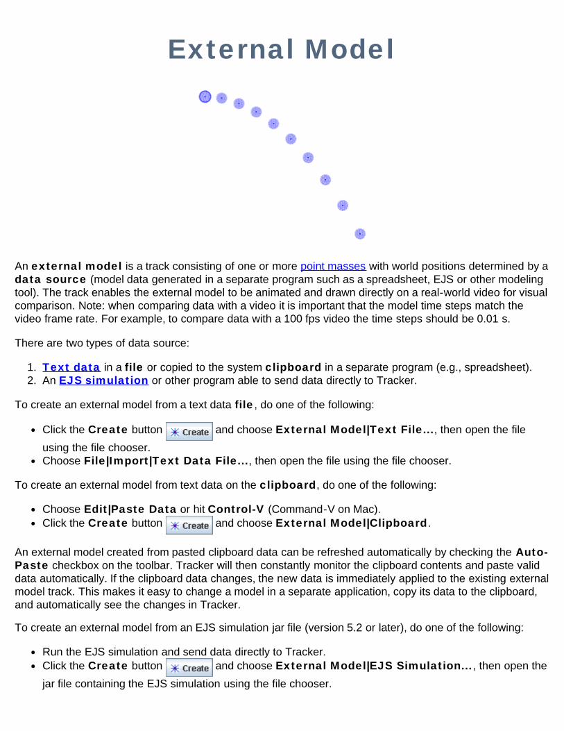
External Model

An external model is a track consisting of one or more point masses with world positions determined by adata source (model data generated in a separate program such as a spreadsheet, EJS or other modelingtool). The track enables the external model to be animated and drawn directly on a real-world video for visualcomparison. Note: when comparing data with a video it is important that the model time steps match thevideo frame rate. For example, to compare data with a 100 fps video the time steps should be 0.01 s.

There are two types of data source:

1. Text data in a file or copied to the system clipboard in a separate program (e.g., spreadsheet).2. An EJS simulation or other program able to send data directly to Tracker.

To create an external model from a text data file, do one of the following:

Click the Create button and choose External Model|Text File..., then open the fileusing the file chooser.Choose File|Import|Text Data File..., then open the file using the file chooser.

To create an external model from text data on the clipboard, do one of the following:

Choose Edit|Paste Data or hit Control-V (Command-V on Mac).Click the Create button and choose External Model|Clipboard.

An external model created from pasted clipboard data can be refreshed automatically by checking the Auto-Paste checkbox on the toolbar. Tracker will then constantly monitor the clipboard contents and paste validdata automatically. If the clipboard data changes, the new data is immediately applied to the existing externalmodel track. This makes it easy to change a model in a separate application, copy its data to the clipboard,and automatically see the changes in Tracker.

To create an external model from an EJS simulation jar file (version 5.2 or later), do one of the following:

Run the EJS simulation and send data directly to Tracker.Click the Create button and choose External Model|EJS Simulation..., then open thejar file containing the EJS simulation using the file chooser.

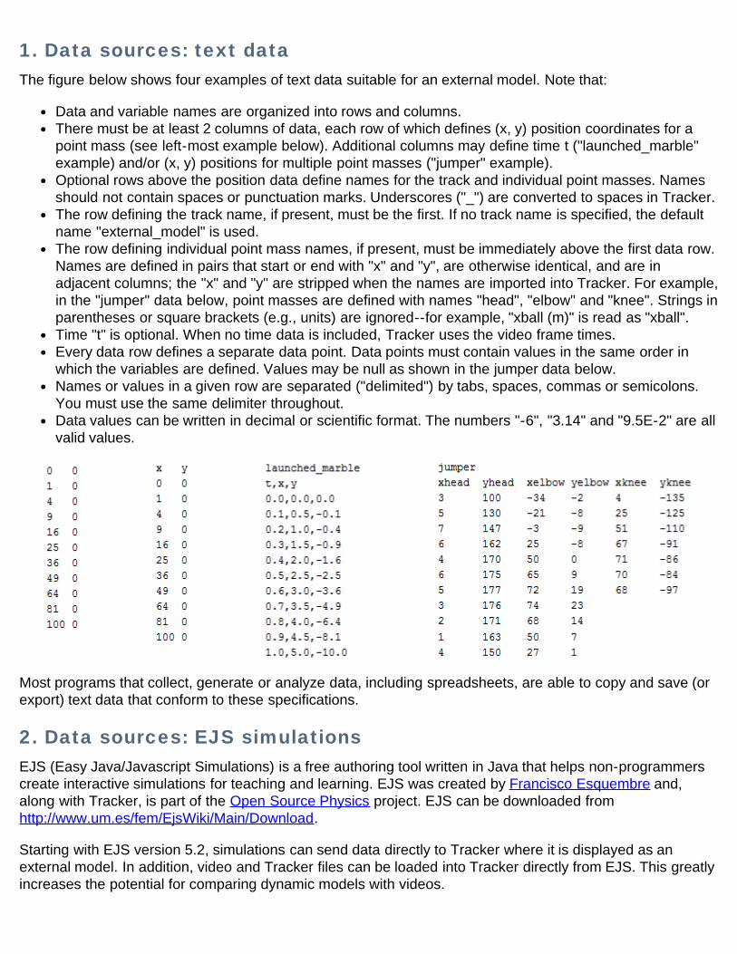
1. Data sources: text dataThe figure below shows four examples of text data suitable for an external model. Note that:

Data and variable names are organized into rows and columns.There must be at least 2 columns of data, each row of which defines (x, y) position coordinates for apoint mass (see left-most example below). Additional columns may define time t ("launched_marble"example) and/or (x, y) positions for multiple point masses ("jumper" example).Optional rows above the position data define names for the track and individual point masses. Namesshould not contain spaces or punctuation marks. Underscores ("_") are converted to spaces in Tracker.The row defining the track name, if present, must be the first. If no track name is specified, the defaultname "external_model" is used.The row defining individual point mass names, if present, must be immediately above the first data row.Names are defined in pairs that start or end with "x" and "y", are otherwise identical, and are inadjacent columns; the "x" and "y" are stripped when the names are imported into Tracker. For example,in the "jumper" data below, point masses are defined with names "head", "elbow" and "knee". Strings inparentheses or square brackets (e.g., units) are ignored--for example, "xball (m)" is read as "xball".Time "t" is optional. When no time data is included, Tracker uses the video frame times.Every data row defines a separate data point. Data points must contain values in the same order inwhich the variables are defined. Values may be null as shown in the jumper data below.Names or values in a given row are separated ("delimited") by tabs, spaces, commas or semicolons.You must use the same delimiter throughout.Data values can be written in decimal or scientific format. The numbers "-6", "3.14" and "9.5E-2" are allvalid values.

Most programs that collect, generate or analyze data, including spreadsheets, are able to copy and save (orexport) text data that conform to these specifications.

2. Data sources: EJS simulationsEJS (Easy Java/Javascript Simulations) is a free authoring tool written in Java that helps non-programmerscreate interactive simulations for teaching and learning. EJS was created by Francisco Esquembre and,along with Tracker, is part of the Open Source Physics project. EJS can be downloaded fromhttp://www.um.es/fem/EjsWiki/Main/Download.

Starting with EJS version 5.2, simulations can send data directly to Tracker where it is displayed as anexternal model. In addition, video and Tracker files can be loaded into Tracker directly from EJS. This greatlyincreases the potential for comparing dynamic models with videos.

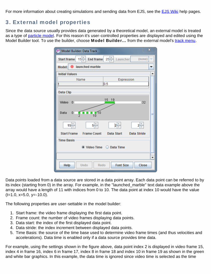
For more information about creating simulations and sending data from EJS, see the EJS Wiki help pages.

3. External model propertiesSince the data source usually provides data generated by a theoretical model, an external model is treatedas a type of particle model. For this reason it's user-controlled properties are displayed and edited using theModel Builder tool. To use the builder, choose Model Builder... from the external model's track menu.

Data points loaded from a data source are stored in a data point array. Each data point can be referred to byits index (starting from 0) in the array. For example, in the "launched_marble" text data example above thearray would have a length of 11 with indices from 0 to 10. The data point at index 10 would have the value(t=1.0, x=5.0, y=-10.0).

The following properties are user-settable in the model builder:

1. Start frame: the video frame displaying the first data point.2. Frame count: the number of video frames displaying data points.3. Data start: the index of the first displayed data point.4. Data stride: the index increment between displayed data points.5. Time Basis: the source of the time base used to determine video frame times (and thus velocities and

accelerations). Data time is enabled only if a data source provides time data.

For example, using the settings shown in the figure above, data point index 2 is displayed in video frame 15,index 4 in frame 16, index 6 in frame 17, index 8 in frame 18 and index 10 in frame 19 as shown in the greenand white bar graphics. In this example, the data time is ignored since video time is selected as the time

basis.

4. External model point and line propertiesThe points defined by a external model are point masses so each has settable mass, color, footprint andmotion vector properties. This also means you can attach measuring tools to the points and add them tocenter of mass tracks just like any other point mass track.

When a external model defines two or more points you can connect them with lines using the Lines item inthe external model's menu. With three or more points choose Close to connect the last point back to thefirst.

5. StampingEach model point can independently create a stamped point mass which clones the model point'scurrent positions. The stamped point mass positions don't move when you change scale. For moreinformation see Stamping a point mass.

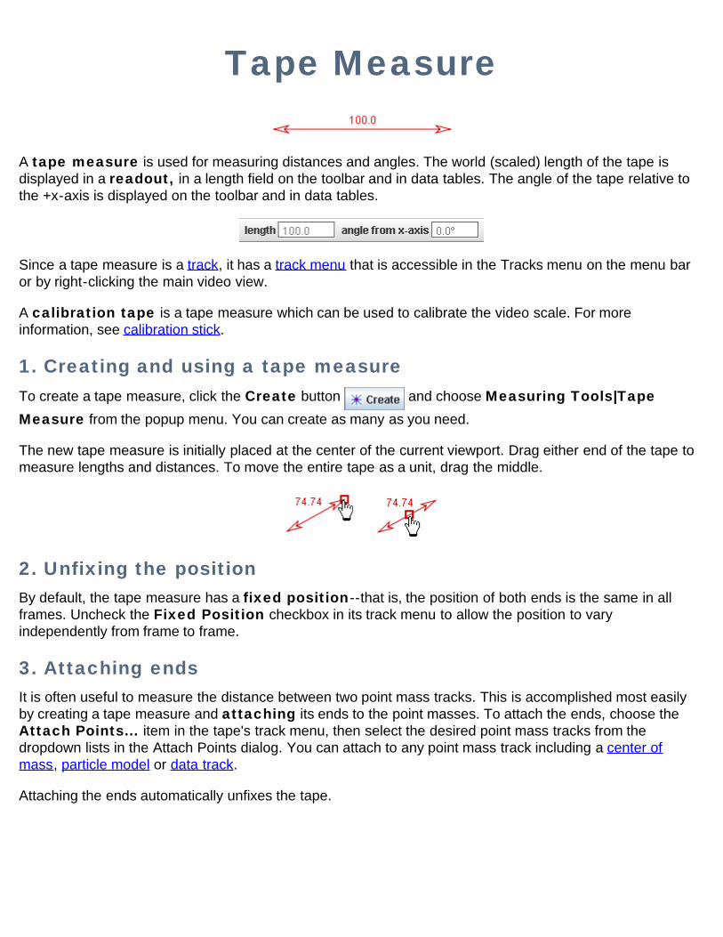
Tape Measure

A tape measure is used for measuring distances and angles. The world (scaled) length of the tape isdisplayed in a readout, in a length field on the toolbar and in data tables. The angle of the tape relative tothe +x-axis is displayed on the toolbar and in data tables.

Since a tape measure is a track, it has a track menu that is accessible in the Tracks menu on the menu baror by right-clicking the main video view.

A calibration tape is a tape measure which can be used to calibrate the video scale. For moreinformation, see calibration stick.

1. Creating and using a tape measureTo create a tape measure, click the Create button and choose Measuring Tools|TapeMeasure from the popup menu. You can create as many as you need.

The new tape measure is initially placed at the center of the current viewport. Drag either end of the tape tomeasure lengths and distances. To move the entire tape as a unit, drag the middle.

2. Unfixing the positionBy default, the tape measure has a fixed position--that is, the position of both ends is the same in allframes. Uncheck the Fixed Position checkbox in its track menu to allow the position to varyindependently from frame to frame.

3. Attaching endsIt is often useful to measure the distance between two point mass tracks. This is accomplished most easilyby creating a tape measure and attaching its ends to the point masses. To attach the ends, choose theAttach Points... item in the tape's track menu, then select the desired point mass tracks from thedropdown lists in the Attach Points dialog. You can attach to any point mass track including a center ofmass, particle model or data track.

Attaching the ends automatically unfixes the tape.

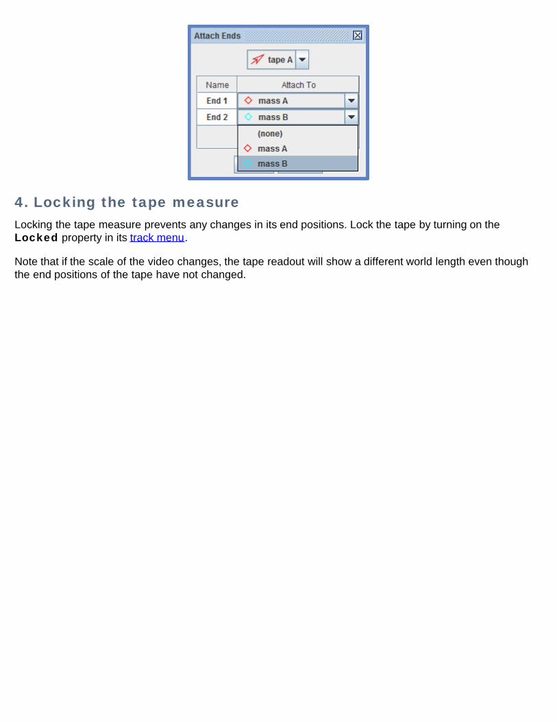
4. Locking the tape measureLocking the tape measure prevents any changes in its end positions. Lock the tape by turning on theLocked property in its track menu.

Note that if the scale of the video changes, the tape readout will show a different world length even thoughthe end positions of the tape have not changed.

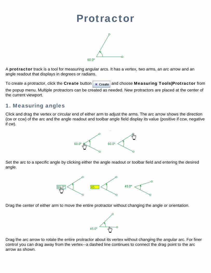
Protractor

A protractor track is a tool for measuring angular arcs. It has a vertex, two arms, an arc arrow and anangle readout that displays in degrees or radians.

To create a protractor, click the Create button and choose Measuring Tools|Protractor fromthe popup menu. Multiple protractors can be created as needed. New protractors are placed at the center ofthe current viewport.

1. Measuring anglesClick and drag the vertex or circular end of either arm to adjust the arms. The arc arrow shows the direction(cw or ccw) of the arc and the angle readout and toolbar angle field display its value (positive if ccw, negativeif cw).

Set the arc to a specific angle by clicking either the angle readout or toolbar field and entering the desiredangle.

Drag the center of either arm to move the entire protractor without changing the angle or orientation.

Drag the arc arrow to rotate the entire protractor about its vertex without changing the angular arc. For finercontrol you can drag away from the vertex--a dashed line continues to connect the drag point to the arcarrow as shown.

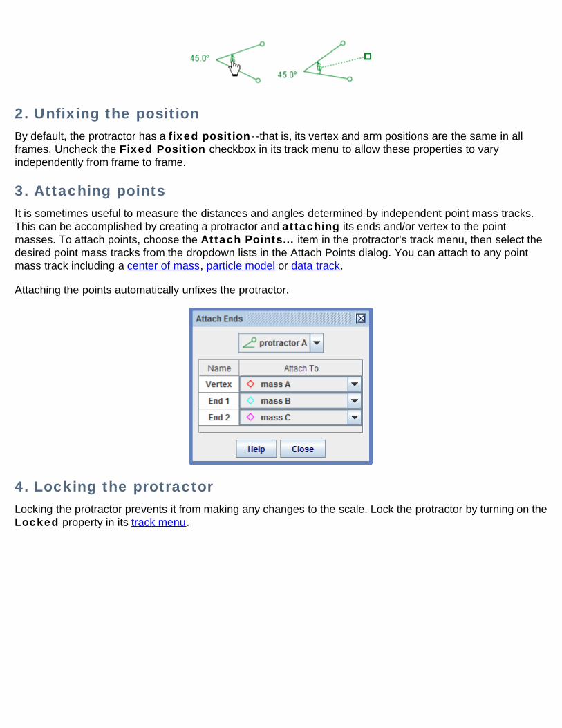
2. Unfixing the positionBy default, the protractor has a fixed position--that is, its vertex and arm positions are the same in allframes. Uncheck the Fixed Position checkbox in its track menu to allow these properties to varyindependently from frame to frame.

3. Attaching pointsIt is sometimes useful to measure the distances and angles determined by independent point mass tracks.This can be accomplished by creating a protractor and attaching its ends and/or vertex to the pointmasses. To attach points, choose the Attach Points... item in the protractor's track menu, then select thedesired point mass tracks from the dropdown lists in the Attach Points dialog. You can attach to any pointmass track including a center of mass, particle model or data track.

Attaching the points automatically unfixes the protractor.

4. Locking the protractorLocking the protractor prevents it from making any changes to the scale. Lock the protractor by turning on theLocked property in its track menu.

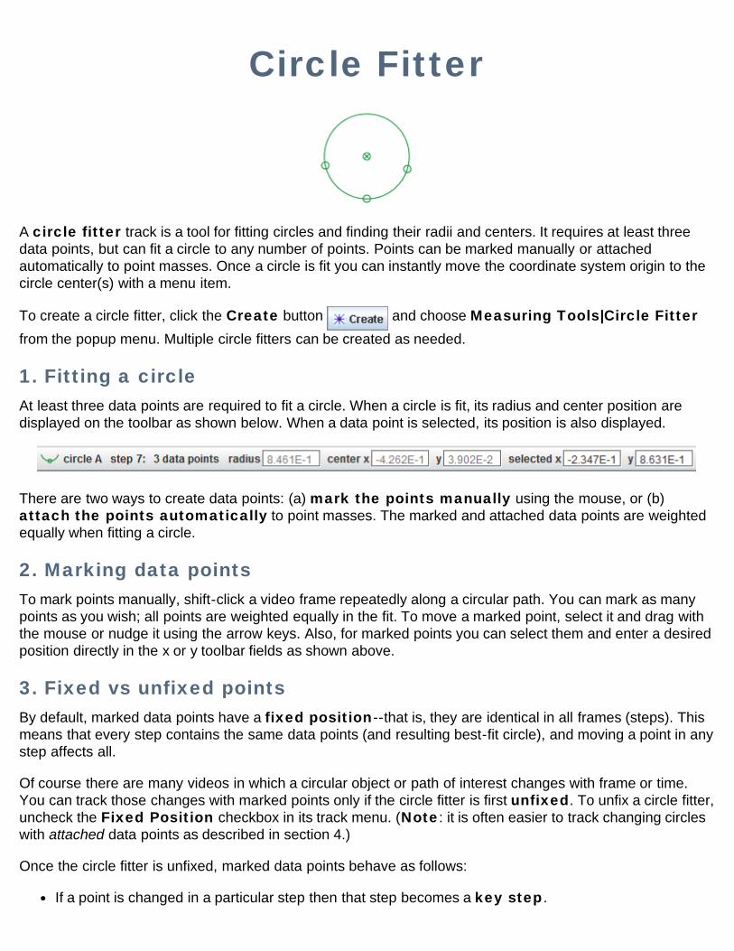
Circle Fitter

A circle fitter track is a tool for fitting circles and finding their radii and centers. It requires at least threedata points, but can fit a circle to any number of points. Points can be marked manually or attachedautomatically to point masses. Once a circle is fit you can instantly move the coordinate system origin to thecircle center(s) with a menu item.

To create a circle fitter, click the Create button and choose Measuring Tools|Circle Fitterfrom the popup menu. Multiple circle fitters can be created as needed.

1. Fitting a circleAt least three data points are required to fit a circle. When a circle is fit, its radius and center position aredisplayed on the toolbar as shown below. When a data point is selected, its position is also displayed.

There are two ways to create data points: (a) mark the points manually using the mouse, or (b)attach the points automatically to point masses. The marked and attached data points are weightedequally when fitting a circle.

2. Marking data pointsTo mark points manually, shift-click a video frame repeatedly along a circular path. You can mark as manypoints as you wish; all points are weighted equally in the fit. To move a marked point, select it and drag withthe mouse or nudge it using the arrow keys. Also, for marked points you can select them and enter a desiredposition directly in the x or y toolbar fields as shown above.

3. Fixed vs unfixed pointsBy default, marked data points have a fixed position--that is, they are identical in all frames (steps). Thismeans that every step contains the same data points (and resulting best-fit circle), and moving a point in anystep affects all.

Of course there are many videos in which a circular object or path of interest changes with frame or time.You can track those changes with marked points only if the circle fitter is first unfixed. To unfix a circle fitter,uncheck the Fixed Position checkbox in its track menu. (Note: it is often easier to track changing circleswith attached data points as described in section 4.)

Once the circle fitter is unfixed, marked data points behave as follows:

If a point is changed in a particular step then that step becomes a key step.

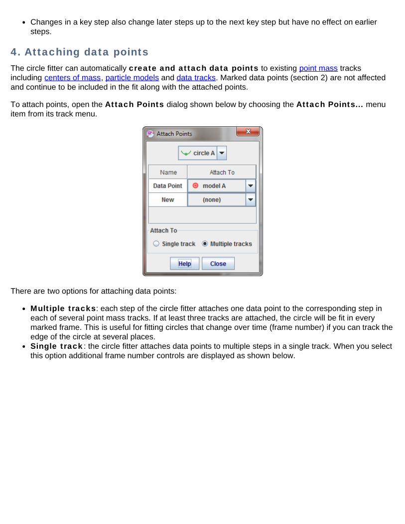
Changes in a key step also change later steps up to the next key step but have no effect on earliersteps.

4. Attaching data pointsThe circle fitter can automatically create and attach data points to existing point mass tracksincluding centers of mass, particle models and data tracks. Marked data points (section 2) are not affectedand continue to be included in the fit along with the attached points.

To attach points, open the Attach Points dialog shown below by choosing the Attach Points... menuitem from its track menu.

There are two options for attaching data points:

Multiple tracks: each step of the circle fitter attaches one data point to the corresponding step ineach of several point mass tracks. If at least three tracks are attached, the circle will be fit in everymarked frame. This is useful for fitting circles that change over time (frame number) if you can track theedge of the circle at several places.Single track: the circle fitter attaches data points to multiple steps in a single track. When you selectthis option additional frame number controls are displayed as shown below.

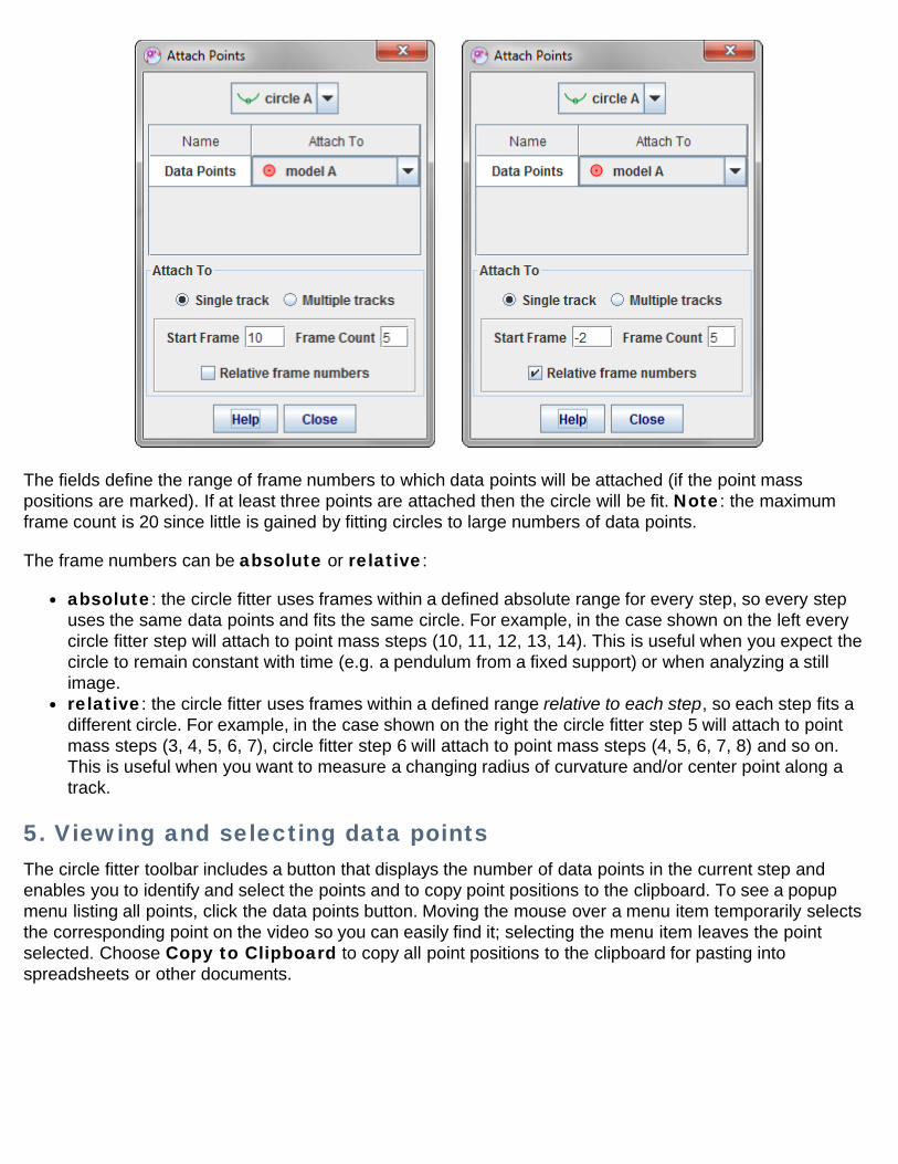
The fields define the range of frame numbers to which data points will be attached (if the point masspositions are marked). If at least three points are attached then the circle will be fit. Note: the maximumframe count is 20 since little is gained by fitting circles to large numbers of data points.

The frame numbers can be absolute or relative:

absolute: the circle fitter uses frames within a defined absolute range for every step, so every stepuses the same data points and fits the same circle. For example, in the case shown on the left everycircle fitter step will attach to point mass steps (10, 11, 12, 13, 14). This is useful when you expect thecircle to remain constant with time (e.g. a pendulum from a fixed support) or when analyzing a stillimage.relative: the circle fitter uses frames within a defined range relative to each step, so each step fits adifferent circle. For example, in the case shown on the right the circle fitter step 5 will attach to pointmass steps (3, 4, 5, 6, 7), circle fitter step 6 will attach to point mass steps (4, 5, 6, 7, 8) and so on.This is useful when you want to measure a changing radius of curvature and/or center point along atrack.

5. Viewing and selecting data pointsThe circle fitter toolbar includes a button that displays the number of data points in the current step andenables you to identify and select the points and to copy point positions to the clipboard. To see a popupmenu listing all points, click the data points button. Moving the mouse over a menu item temporarily selectsthe corresponding point on the video so you can easily find it; selecting the menu item leaves the pointselected. Choose Copy to Clipboard to copy all point positions to the clipboard for pasting intospreadsheets or other documents.

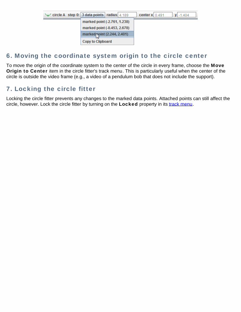
6. Moving the coordinate system origin to the circle centerTo move the origin of the coordinate system to the center of the circle in every frame, choose the MoveOrigin to Center item in the circle fitter's track menu. This is particularly useful when the center of thecircle is outside the video frame (e.g., a video of a pendulum bob that does not include the support).

7. Locking the circle fitterLocking the circle fitter prevents any changes to the marked data points. Attached points can still affect thecircle, however. Lock the circle fitter by turning on the Locked property in its track menu.

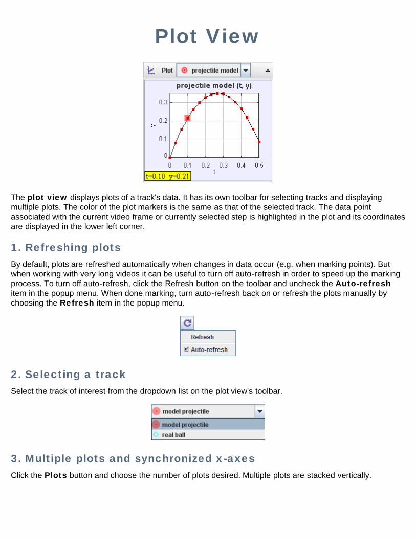
Plot View

The plot view displays plots of a track's data. It has its own toolbar for selecting tracks and displayingmultiple plots. The color of the plot markers is the same as that of the selected track. The data pointassociated with the current video frame or currently selected step is highlighted in the plot and its coordinatesare displayed in the lower left corner.

1. Refreshing plotsBy default, plots are refreshed automatically when changes in data occur (e.g. when marking points). Butwhen working with very long videos it can be useful to turn off auto-refresh in order to speed up the markingprocess. To turn off auto-refresh, click the Refresh button on the toolbar and uncheck the Auto-refreshitem in the popup menu. When done marking, turn auto-refresh back on or refresh the plots manually bychoosing the Refresh item in the popup menu.

2. Selecting a trackSelect the track of interest from the dropdown list on the plot view's toolbar.

3. Multiple plots and synchronized x-axesClick the Plots button and choose the number of plots desired. Multiple plots are stacked vertically.

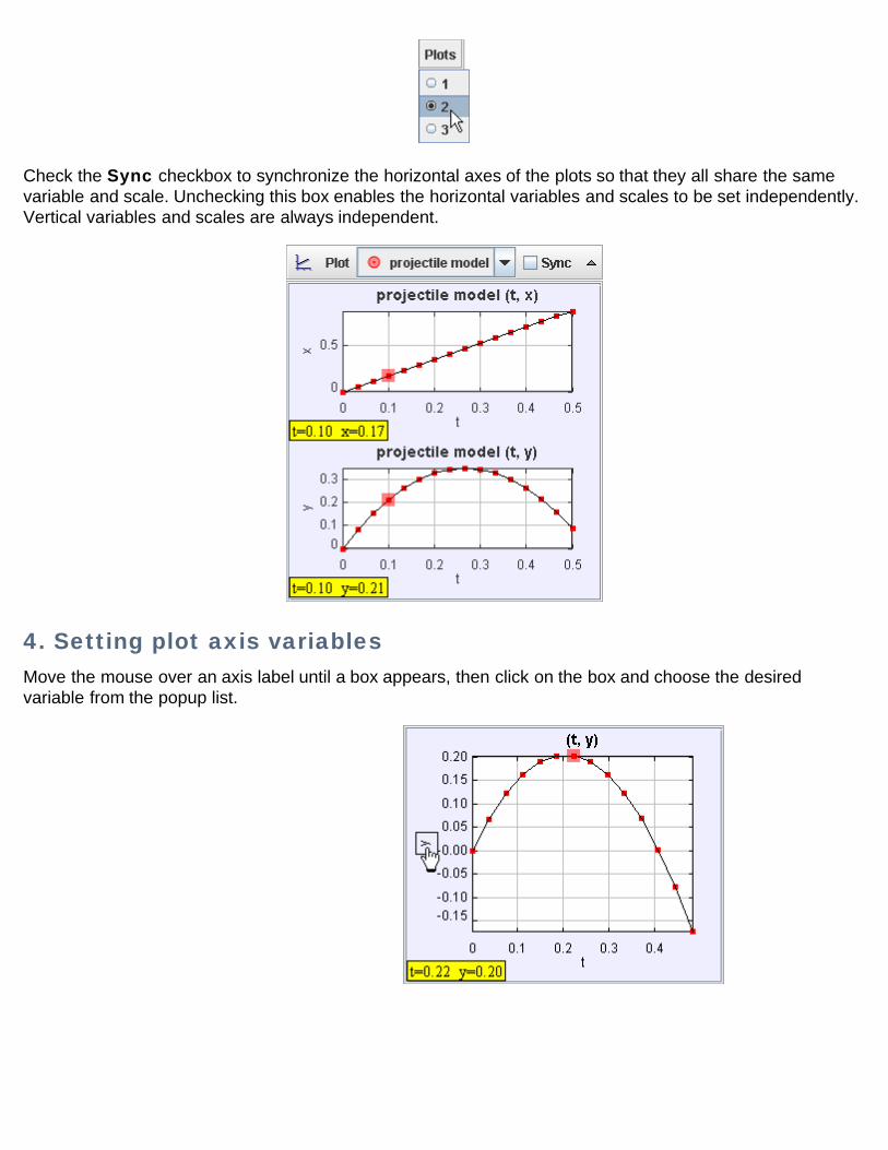
Check the Sync checkbox to synchronize the horizontal axes of the plots so that they all share the samevariable and scale. Unchecking this box enables the horizontal variables and scales to be set independently.Vertical variables and scales are always independent.

4. Setting plot axis variablesMove the mouse over an axis label until a box appears, then click on the box and choose the desiredvariable from the popup list.

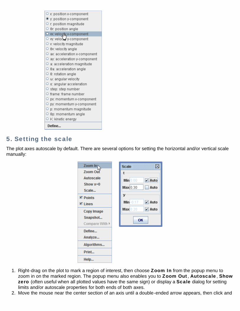
5. Setting the scaleThe plot axes autoscale by default. There are several options for setting the horizontal and/or vertical scalemanually:

1. Right-drag on the plot to mark a region of interest, then choose Zoom In from the popup menu tozoom in on the marked region. The popup menu also enables you to Zoom Out, Autoscale, Showzero (often useful when all plotted values have the same sign) or display a Scale dialog for settinglimits and/or autoscale properties for both ends of both axes.

2. Move the mouse near the center section of an axis until a double-ended arrow appears, then click and

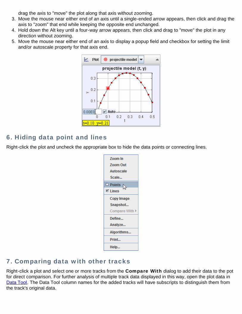
drag the axis to "move" the plot along that axis without zooming.3. Move the mouse near either end of an axis until a single-ended arrow appears, then click and drag the

axis to "zoom" that end while keeping the opposite end unchanged.4. Hold down the Alt key until a four-way arrow appears, then click and drag to "move" the plot in any

direction without zooming.5. Move the mouse near either end of an axis to display a popup field and checkbox for setting the limit

and/or autoscale property for that axis end.

6. Hiding data point and linesRight-click the plot and uncheck the appropriate box to hide the data points or connecting lines.

7. Comparing data with other tracksRight-click a plot and select one or more tracks from the Compare With dialog to add their data to the potfor direct comparison. For further analysis of multiple track data displayed in this way, open the plot data inData Tool. The Data Tool column names for the added tracks will have subscripts to distinguish them fromthe track's original data.

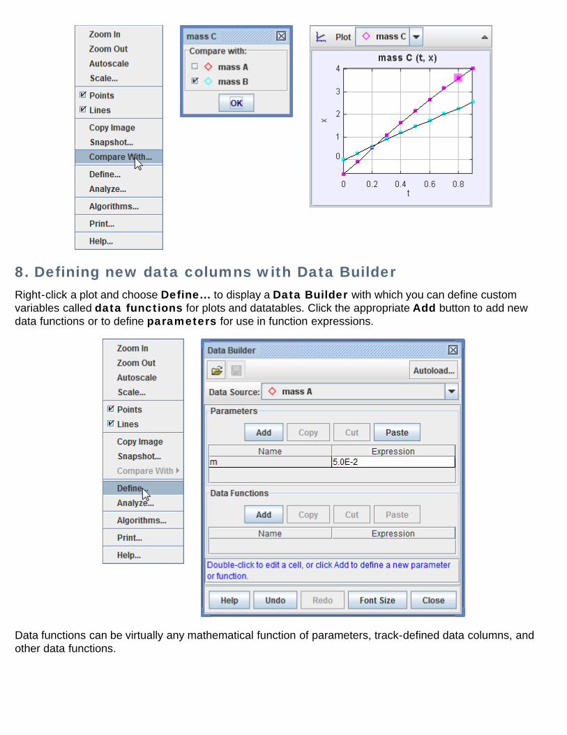
8. Defining new data columns with Data BuilderRight-click a plot and choose Define... to display a Data Builder with which you can define customvariables called data functions for plots and datatables. Click the appropriate Add button to add newdata functions or to define parameters for use in function expressions.

Data functions can be virtually any mathematical function of parameters, track-defined data columns, andother data functions.

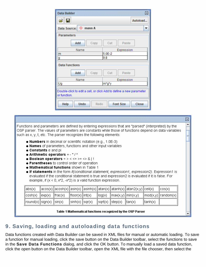
9. Saving, loading and autoloading data functionsData functions created with Data Builder can be saved in XML files for manual or automatic loading. To savea function for manual loading, click the save button on the Data Builder toolbar, select the functions to savein the Save Data Functions dialog, and click the OK button. To manually load a saved data function,click the open button on the Data Builder toolbar, open the XML file with the file chooser, then select the

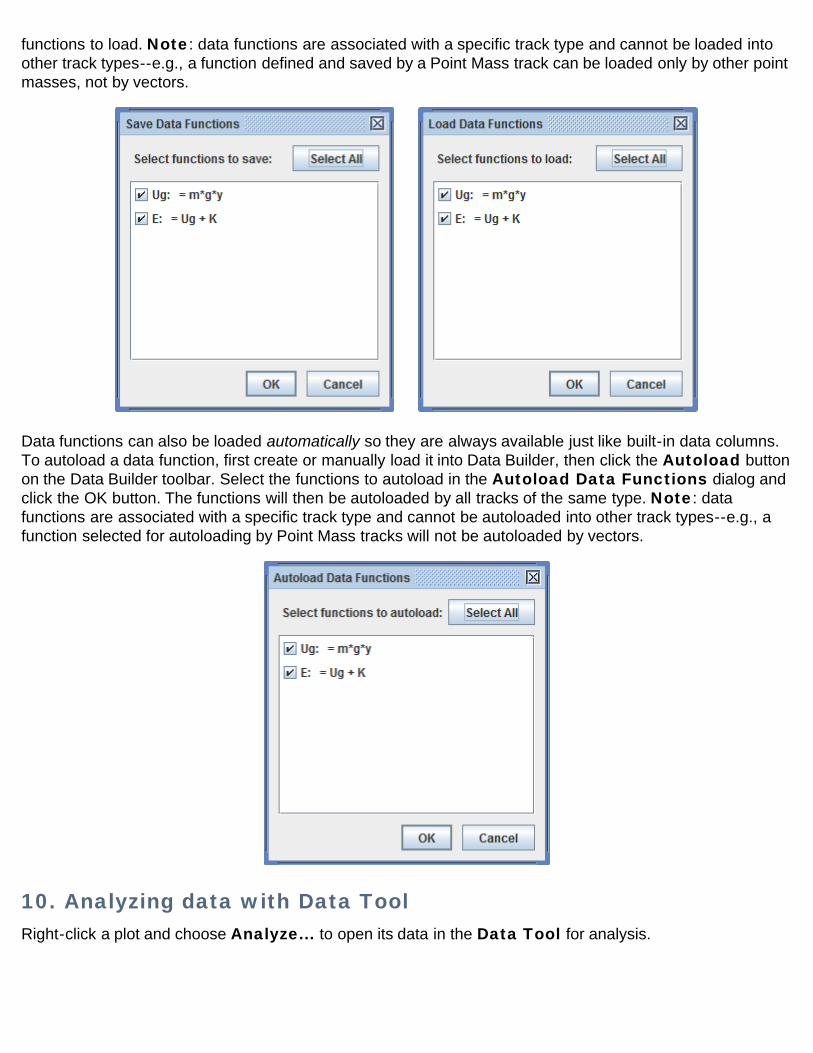
functions to load. Note: data functions are associated with a specific track type and cannot be loaded intoother track types--e.g., a function defined and saved by a Point Mass track can be loaded only by other pointmasses, not by vectors.

Data functions can also be loaded automatically so they are always available just like built-in data columns.To autoload a data function, first create or manually load it into Data Builder, then click the Autoload buttonon the Data Builder toolbar. Select the functions to autoload in the Autoload Data Functions dialog andclick the OK button. The functions will then be autoloaded by all tracks of the same type. Note: datafunctions are associated with a specific track type and cannot be autoloaded into other track types--e.g., afunction selected for autoloading by Point Mass tracks will not be autoloaded by vectors.

10. Analyzing data with Data ToolRight-click a plot and choose Analyze... to open its data in the Data Tool for analysis.

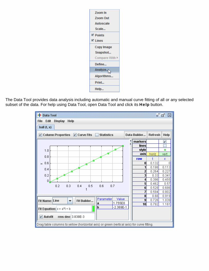
The Data Tool provides data analysis including automatic and manual curve fitting of all or any selectedsubset of the data. For help using Data Tool, open Data Tool and click its Help button.

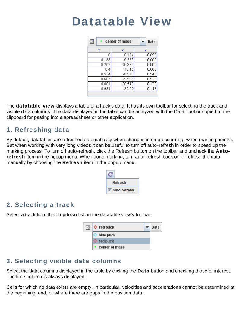
Datatable View

The datatable view displays a table of a track's data. It has its own toolbar for selecting the track andvisible data columns. The data displayed in the table can be analyzed with the Data Tool or copied to theclipboard for pasting into a spreadsheet or other application.

1. Refreshing dataBy default, datatables are refreshed automatically when changes in data occur (e.g. when marking points).But when working with very long videos it can be useful to turn off auto-refresh in order to speed up themarking process. To turn off auto-refresh, click the Refresh button on the toolbar and uncheck the Auto-refresh item in the popup menu. When done marking, turn auto-refresh back on or refresh the datamanually by choosing the Refresh item in the popup menu.

2. Selecting a trackSelect a track from the dropdown list on the datatable view's toolbar.

3. Selecting visible data columnsSelect the data columns displayed in the table by clicking the Data button and checking those of interest.The time column is always displayed.

Cells for which no data exists are empty. In particular, velocities and accelerations cannot be determined atthe beginning, end, or where there are gaps in the position data.

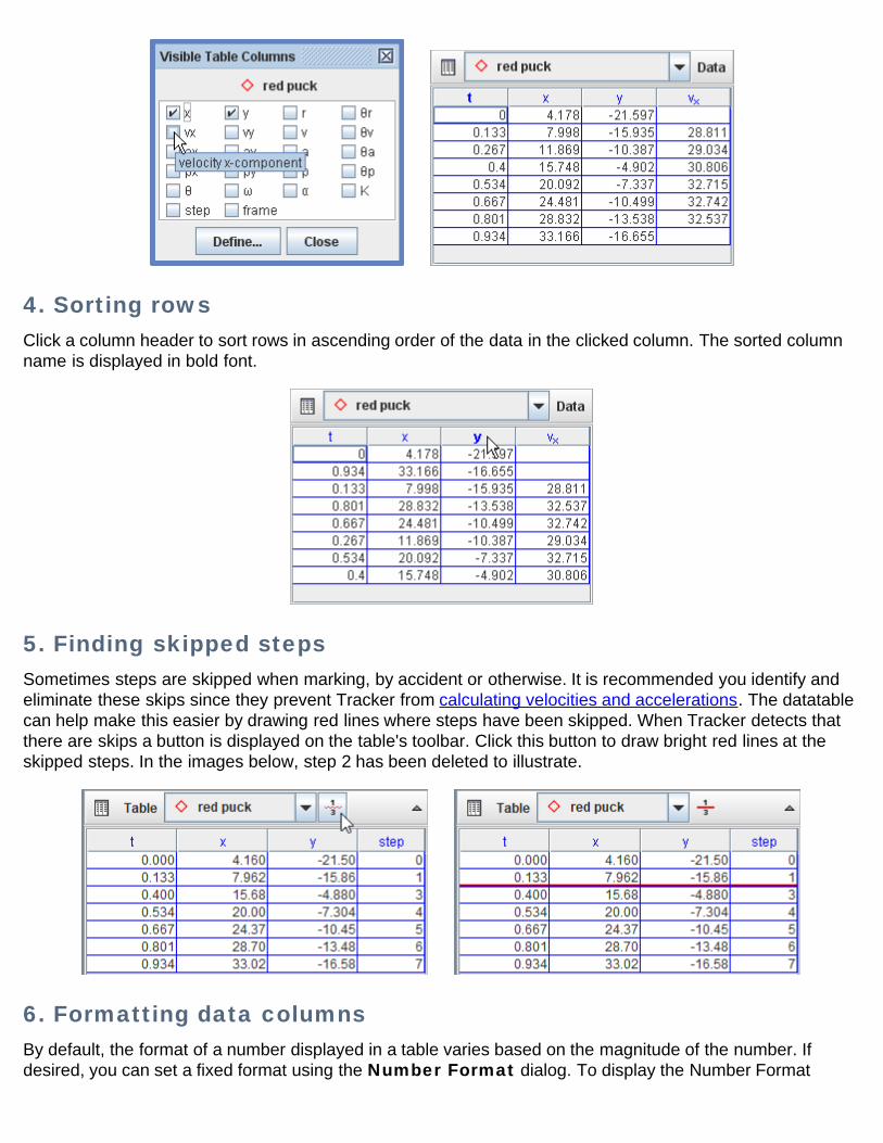
4. Sorting rowsClick a column header to sort rows in ascending order of the data in the clicked column. The sorted columnname is displayed in bold font.

5. Finding skipped stepsSometimes steps are skipped when marking, by accident or otherwise. It is recommended you identify andeliminate these skips since they prevent Tracker from calculating velocities and accelerations. The datatablecan help make this easier by drawing red lines where steps have been skipped. When Tracker detects thatthere are skips a button is displayed on the table's toolbar. Click this button to draw bright red lines at theskipped steps. In the images below, step 2 has been deleted to illustrate.

6. Formatting data columnsBy default, the format of a number displayed in a table varies based on the magnitude of the number. Ifdesired, you can set a fixed format using the Number Format dialog. To display the Number Format

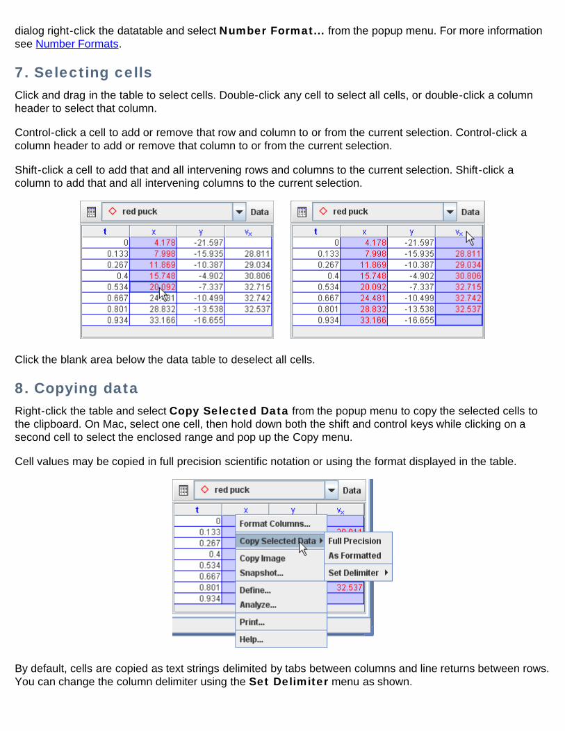
dialog right-click the datatable and select Number Format... from the popup menu. For more informationsee Number Formats.

7. Selecting cellsClick and drag in the table to select cells. Double-click any cell to select all cells, or double-click a columnheader to select that column.

Control-click a cell to add or remove that row and column to or from the current selection. Control-click acolumn header to add or remove that column to or from the current selection.

Shift-click a cell to add that and all intervening rows and columns to the current selection. Shift-click acolumn to add that and all intervening columns to the current selection.

Click the blank area below the data table to deselect all cells.

8. Copying dataRight-click the table and select Copy Selected Data from the popup menu to copy the selected cells tothe clipboard. On Mac, select one cell, then hold down both the shift and control keys while clicking on asecond cell to select the enclosed range and pop up the Copy menu.

Cell values may be copied in full precision scientific notation or using the format displayed in the table.

By default, cells are copied as text strings delimited by tabs between columns and line returns between rows.You can change the column delimiter using the Set Delimiter menu as shown.

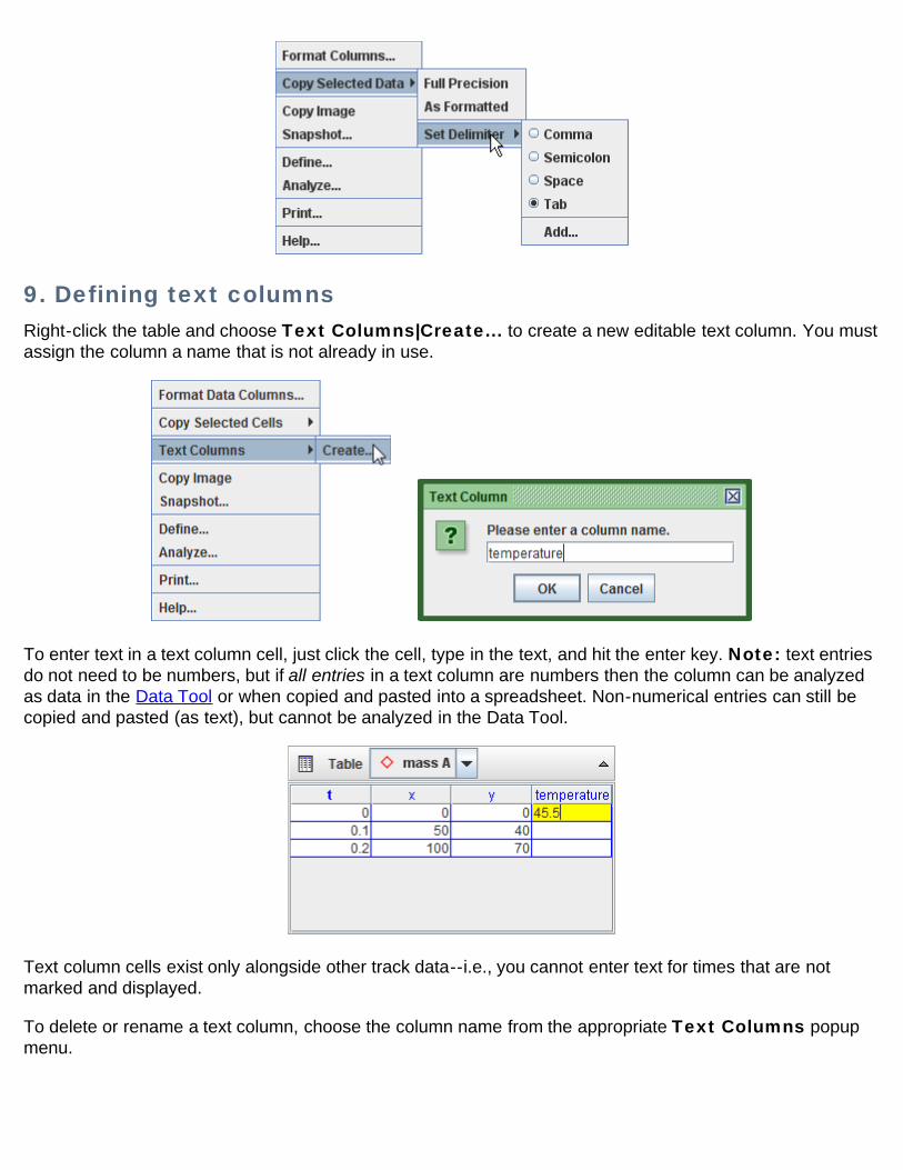
9. Defining text columnsRight-click the table and choose Text Columns|Create... to create a new editable text column. You mustassign the column a name that is not already in use.

To enter text in a text column cell, just click the cell, type in the text, and hit the enter key. Note: text entriesdo not need to be numbers, but if all entries in a text column are numbers then the column can be analyzedas data in the Data Tool or when copied and pasted into a spreadsheet. Non-numerical entries can still becopied and pasted (as text), but cannot be analyzed in the Data Tool.

Text column cells exist only alongside other track data--i.e., you cannot enter text for times that are notmarked and displayed.

To delete or rename a text column, choose the column name from the appropriate Text Columns popupmenu.

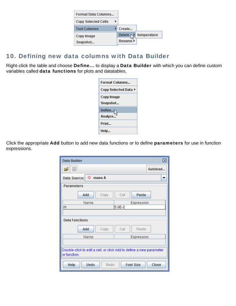
10. Defining new data columns with Data BuilderRight-click the table and choose Define... to display a Data Builder with which you can define customvariables called data functions for plots and datatables.

Click the appropriate Add button to add new data functions or to define parameters for use in functionexpressions.

Data functions can be virtually any mathematical function of parameters, track-defined data columns, andother data functions.

11. Saving, loading and autoloading data functionsData functions created with Data Builder can be saved in XML files for manual or automatic loading. To save

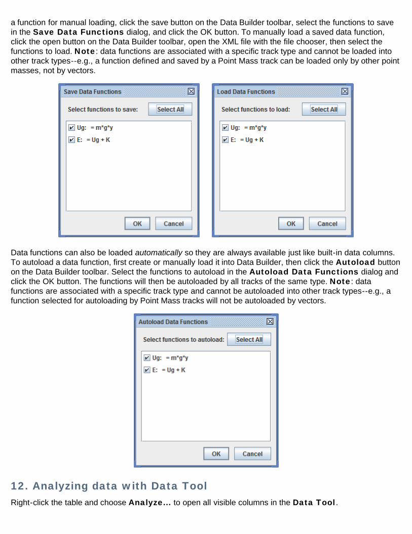
a function for manual loading, click the save button on the Data Builder toolbar, select the functions to savein the Save Data Functions dialog, and click the OK button. To manually load a saved data function,click the open button on the Data Builder toolbar, open the XML file with the file chooser, then select thefunctions to load. Note: data functions are associated with a specific track type and cannot be loaded intoother track types--e.g., a function defined and saved by a Point Mass track can be loaded only by other pointmasses, not by vectors.

Data functions can also be loaded automatically so they are always available just like built-in data columns.To autoload a data function, first create or manually load it into Data Builder, then click the Autoload buttonon the Data Builder toolbar. Select the functions to autoload in the Autoload Data Functions dialog andclick the OK button. The functions will then be autoloaded by all tracks of the same type. Note: datafunctions are associated with a specific track type and cannot be autoloaded into other track types--e.g., afunction selected for autoloading by Point Mass tracks will not be autoloaded by vectors.

12. Analyzing data with Data ToolRight-click the table and choose Analyze... to open all visible columns in the Data Tool.

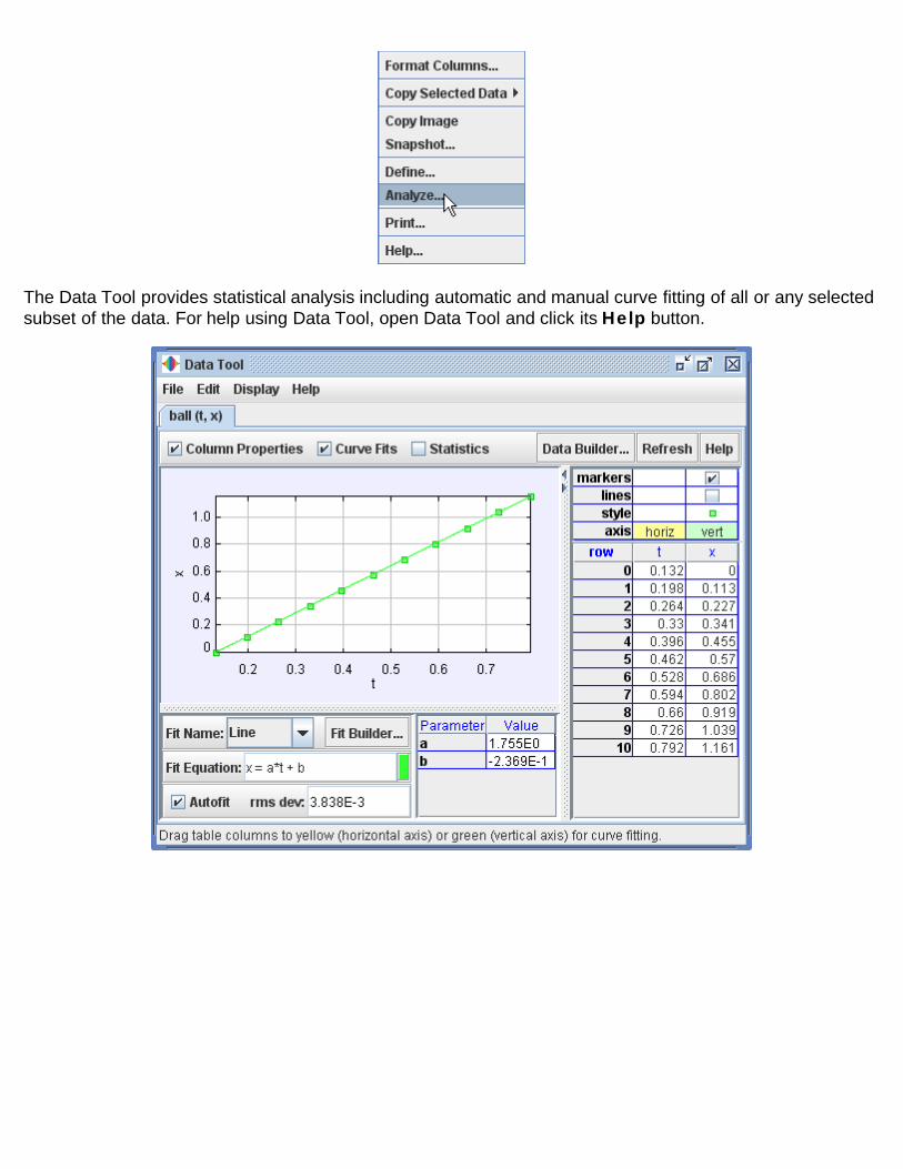
The Data Tool provides statistical analysis including automatic and manual curve fitting of all or any selectedsubset of the data. For help using Data Tool, open Data Tool and click its Help button.

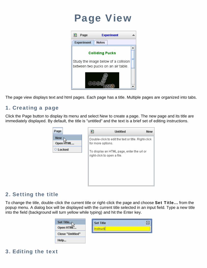
Page View

The page view displays text and html pages. Each page has a title. Multiple pages are organized into tabs.

1. Creating a pageClick the Page button to display its menu and select New to create a page. The new page and its title areimmediately displayed. By default, the title is "untitled" and the text is a brief set of editing instructions.

2. Setting the titleTo change the title, double-click the current title or right-click the page and choose Set Title... from thepopup menu. A dialog box will be displayed with the current title selected in an input field. Type a new titleinto the field (background will turn yellow while typing) and hit the Enter key.

3. Editing the text

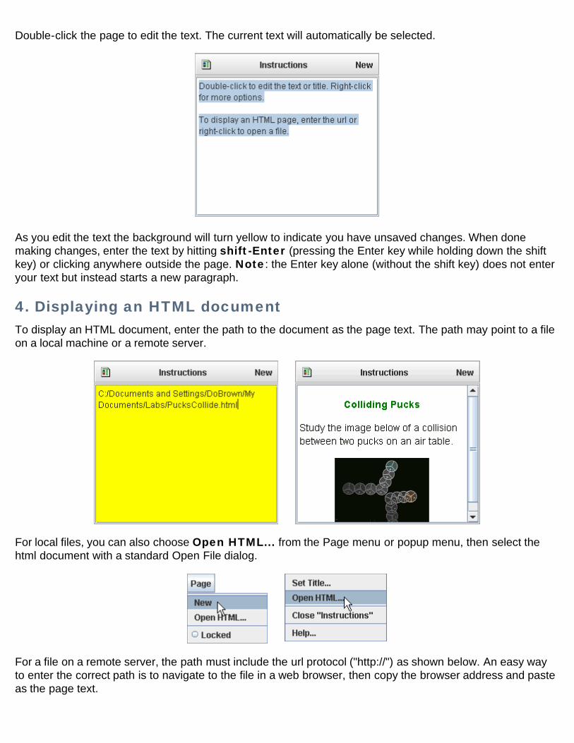
Double-click the page to edit the text. The current text will automatically be selected.

As you edit the text the background will turn yellow to indicate you have unsaved changes. When donemaking changes, enter the text by hitting shift-Enter (pressing the Enter key while holding down the shiftkey) or clicking anywhere outside the page. Note: the Enter key alone (without the shift key) does not enteryour text but instead starts a new paragraph.

4. Displaying an HTML documentTo display an HTML document, enter the path to the document as the page text. The path may point to a fileon a local machine or a remote server.

For local files, you can also choose Open HTML... from the Page menu or popup menu, then select thehtml document with a standard Open File dialog.

For a file on a remote server, the path must include the url protocol ("http://") as shown below. An easy wayto enter the correct path is to navigate to the file in a web browser, then copy the browser address and pasteas the page text.

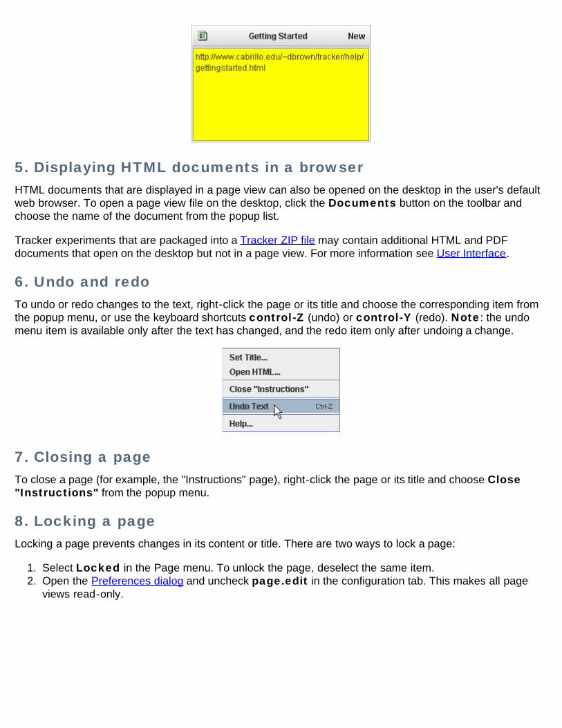
5. Displaying HTML documents in a browserHTML documents that are displayed in a page view can also be opened on the desktop in the user's defaultweb browser. To open a page view file on the desktop, click the Documents button on the toolbar andchoose the name of the document from the popup list.

Tracker experiments that are packaged into a Tracker ZIP file may contain additional HTML and PDFdocuments that open on the desktop but not in a page view. For more information see User Interface.

6. Undo and redoTo undo or redo changes to the text, right-click the page or its title and choose the corresponding item fromthe popup menu, or use the keyboard shortcuts control-Z (undo) or control-Y (redo). Note: the undomenu item is available only after the text has changed, and the redo item only after undoing a change.

7. Closing a pageTo close a page (for example, the "Instructions" page), right-click the page or its title and choose Close"Instructions" from the popup menu.

8. Locking a pageLocking a page prevents changes in its content or title. There are two ways to lock a page:

1. Select Locked in the Page menu. To unlock the page, deselect the same item.2. Open the Preferences dialog and uncheck page.edit in the configuration tab. This makes all page

views read-only.

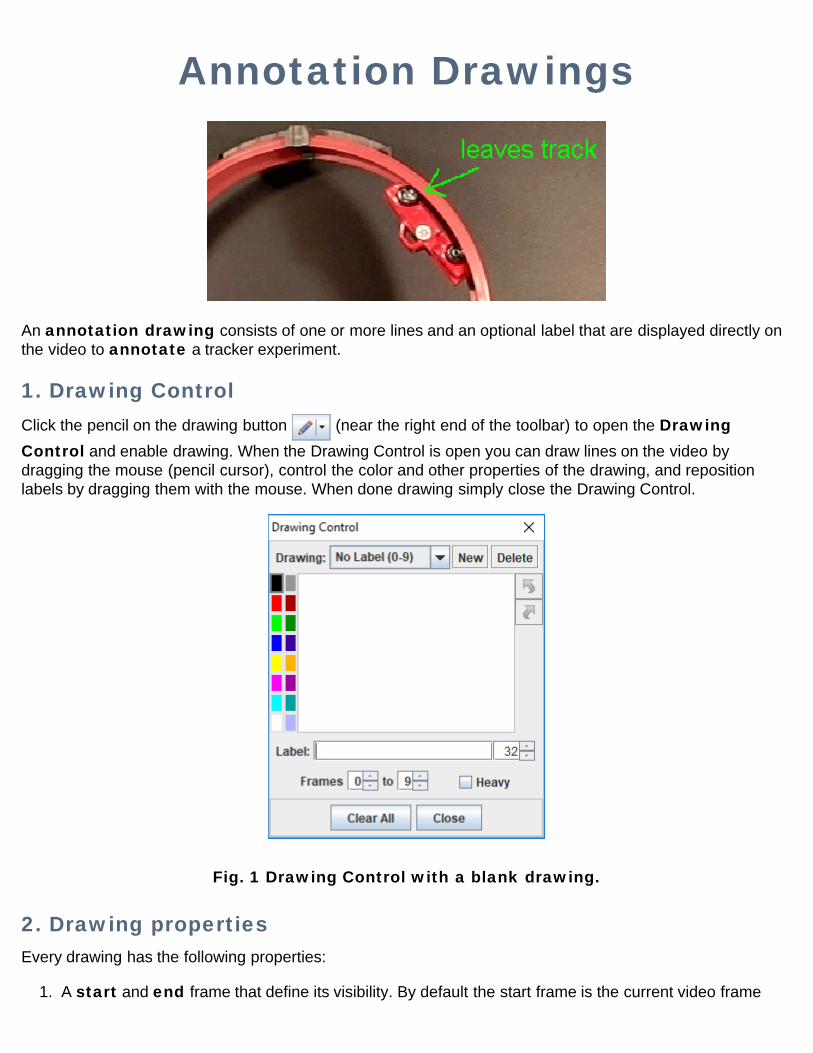
Annotation Drawings

An annotation drawing consists of one or more lines and an optional label that are displayed directly onthe video to annotate a tracker experiment.

1. Drawing ControlClick the pencil on the drawing button (near the right end of the toolbar) to open the DrawingControl and enable drawing. When the Drawing Control is open you can draw lines on the video bydragging the mouse (pencil cursor), control the color and other properties of the drawing, and repositionlabels by dragging them with the mouse. When done drawing simply close the Drawing Control.

Fig. 1 Drawing Control with a blank drawing.

2. Drawing propertiesEvery drawing has the following properties:

1. A start and end frame that define its visibility. By default the start frame is the current video frame

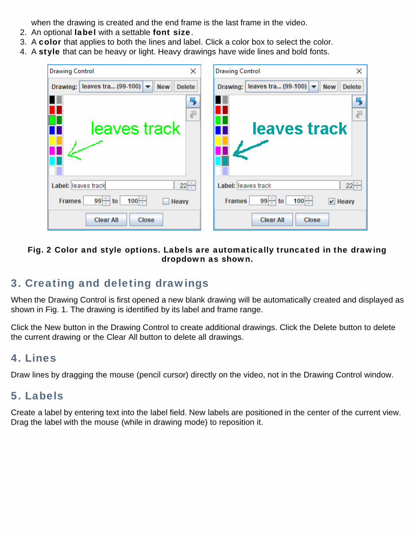
when the drawing is created and the end frame is the last frame in the video.2. An optional label with a settable font size.3. A color that applies to both the lines and label. Click a color box to select the color.4. A style that can be heavy or light. Heavy drawings have wide lines and bold fonts.

Fig. 2 Color and style options. Labels are automatically truncated in the drawingdropdown as shown.

3. Creating and deleting drawingsWhen the Drawing Control is first opened a new blank drawing will be automatically created and displayed asshown in Fig. 1. The drawing is identified by its label and frame range.

Click the New button in the Drawing Control to create additional drawings. Click the Delete button to deletethe current drawing or the Clear All button to delete all drawings.

4. LinesDraw lines by dragging the mouse (pencil cursor) directly on the video, not in the Drawing Control window.

5. LabelsCreate a label by entering text into the label field. New labels are positioned in the center of the current view.Drag the label with the mouse (while in drawing mode) to reposition it.

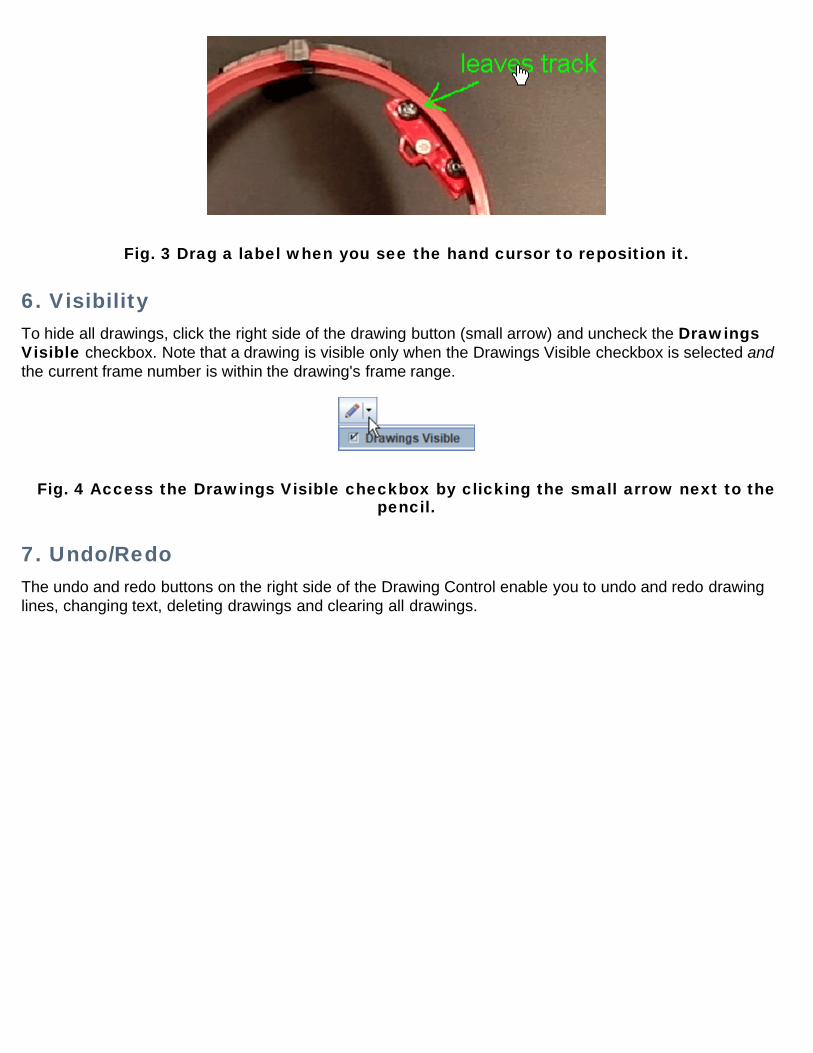
Fig. 3 Drag a label when you see the hand cursor to reposition it.

6. VisibilityTo hide all drawings, click the right side of the drawing button (small arrow) and uncheck the DrawingsVisible checkbox. Note that a drawing is visible only when the Drawings Visible checkbox is selected andthe current frame number is within the drawing's frame range.

Fig. 4 Access the Drawings Visible checkbox by clicking the small arrow next to thepencil.

7. Undo/RedoThe undo and redo buttons on the right side of the Drawing Control enable you to undo and redo drawinglines, changing text, deleting drawings and clearing all drawings.

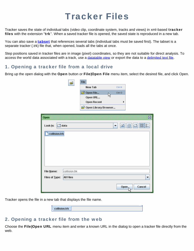
Tracker FilesTracker saves the state of individual tabs (video clip, coordinate system, tracks and views) in xml-based trackerfiles with the extension "trk". When a saved tracker file is opened, the saved state is reproduced in a new tab.

You can also save a tabset that references several tabs (individual tabs must be saved first). The tabset is aseparate tracker (.trk) file that, when opened, loads all the tabs at once.

Step positions saved in tracker files are in image (pixel) coordinates, so they are not suitable for direct analysis. Toaccess the world data associated with a track, use a datatable view or export the data to a delimited text file.

1. Opening a tracker file from a local driveBring up the open dialog with the Open button or File|Open File menu item, select the desired file, and click Open.

Tracker opens the file in a new tab that displays the file name.

2. Opening a tracker file from the webChoose the File|Open URL menu item and enter a known URL in the dialog to open a tracker file directly from theweb.

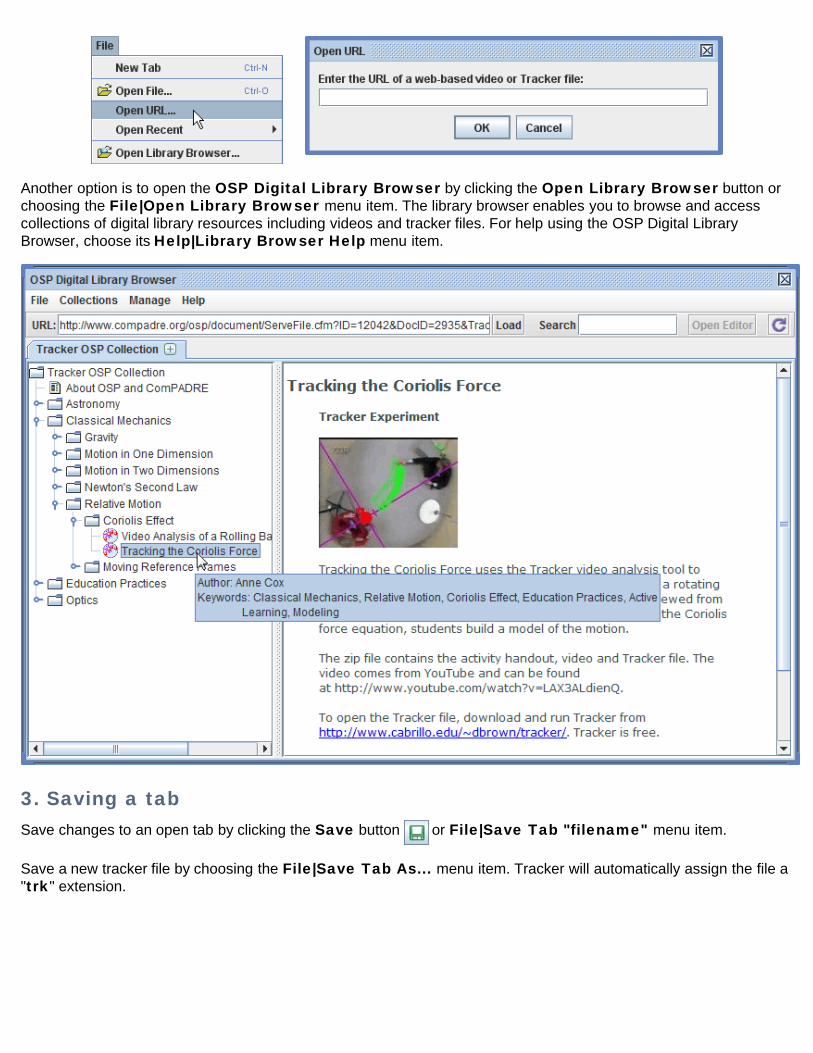
Another option is to open the OSP Digital Library Browser by clicking the Open Library Browser button orchoosing the File|Open Library Browser menu item. The library browser enables you to browse and accesscollections of digital library resources including videos and tracker files. For help using the OSP Digital LibraryBrowser, choose its Help|Library Browser Help menu item.

3. Saving a tabSave changes to an open tab by clicking the Save button or File|Save Tab "filename" menu item.

Save a new tracker file by choosing the File|Save Tab As... menu item. Tracker will automatically assign the file a"trk" extension.

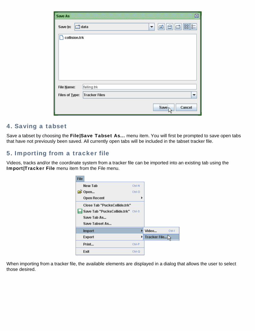
4. Saving a tabsetSave a tabset by choosing the File|Save Tabset As... menu item. You will first be prompted to save open tabsthat have not previously been saved. All currently open tabs will be included in the tabset tracker file.

5. Importing from a tracker fileVideos, tracks and/or the coordinate system from a tracker file can be imported into an existing tab using theImport|Tracker File menu item from the File menu.

When importing from a tracker file, the available elements are displayed in a dialog that allows the user to selectthose desired.

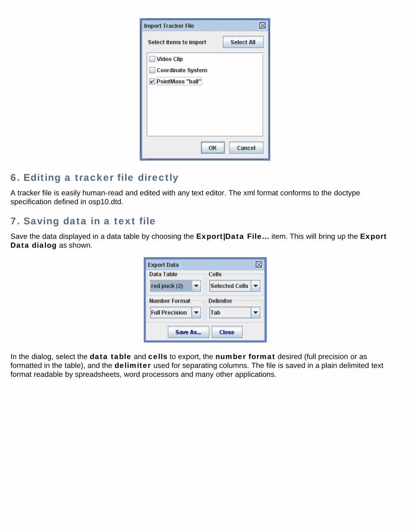
6. Editing a tracker file directlyA tracker file is easily human-read and edited with any text editor. The xml format conforms to the doctypespecification defined in osp10.dtd.

7. Saving data in a text fileSave the data displayed in a data table by choosing the Export|Data File... item. This will bring up the ExportData dialog as shown.

In the dialog, select the data table and cells to export, the number format desired (full precision or asformatted in the table), and the delimiter used for separating columns. The file is saved in a plain delimited textformat readable by spreadsheets, word processors and many other applications.

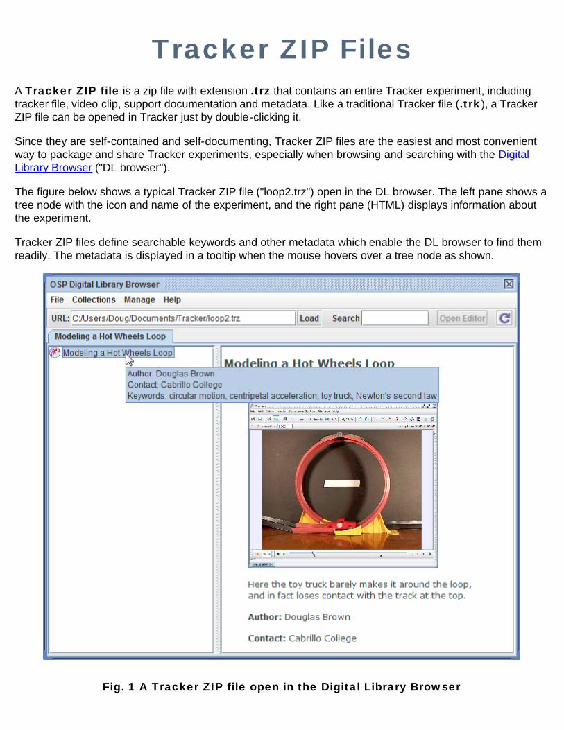
Tracker ZIP FilesA Tracker ZIP file is a zip file with extension .trz that contains an entire Tracker experiment, includingtracker file, video clip, support documentation and metadata. Like a traditional Tracker file (.trk), a TrackerZIP file can be opened in Tracker just by double-clicking it.

Since they are self-contained and self-documenting, Tracker ZIP files are the easiest and most convenientway to package and share Tracker experiments, especially when browsing and searching with the DigitalLibrary Browser ("DL browser").

The figure below shows a typical Tracker ZIP file ("loop2.trz") open in the DL browser. The left pane shows atree node with the icon and name of the experiment, and the right pane (HTML) displays information aboutthe experiment.

Tracker ZIP files define searchable keywords and other metadata which enable the DL browser to find themreadily. The metadata is displayed in a tooltip when the mouse hovers over a tree node as shown.

Fig. 1 A Tracker ZIP file open in the Digital Library Browser

1. Anatomy of a Tracker ZIP fileA Tracker ZIP file is a compressed zip file containing resource files that share a common naming schemeand define all data and metadata used by the DL browser. For example, the file "loop2.trz" contains thefollowing:

1. A tracker data file "loop2.trk"2. A video file "loop2.flv"3. An HTML information file "loop2_info.html" (described below)4. A thumbnnail image file "loop2_thumbnail.png"

Note that all of these files have names that start with "loop2".

HTML information files use standard HTML code in the <head> section to define the title (tree nodename) and metadata for the Tracker ZIP. For example, the HTML information file "loop2_info.html" includesthe following:

<meta name="author" content="Douglas Brown"><meta name="contact" content="Cabrillo College"><meta name="keywords" content="circular motion, centripetal acceleration, toy truck, Newton'ssecond law"><title>Modeling a Hot Wheels Loop</title>

Supplemental HTML, PDF and other support files (with associated images) may also be added toa Tracker ZIP file. These are displayed in Tracker itself (see page views) and/or in separate desktop viewers.They do not have to conform to the naming conventions above.

Tracker ZIP files can be created with any HTML editor and zip utility, but it is much easier to export themfrom Tracker in a single step as described below.

2. Exporting a Tracker ZIP fileClick the Export Tracker ZIP button on the toolbar or choose the File|Export Tracker ZIP menuitem to open a dialog with fields and controls for defining and saving a ZIP file for the currently selected tab.

The figure below shows the Export Tracker ZIP dialog with fields completed prior to exporting the file"loop2.trz" open in the DL browser above.

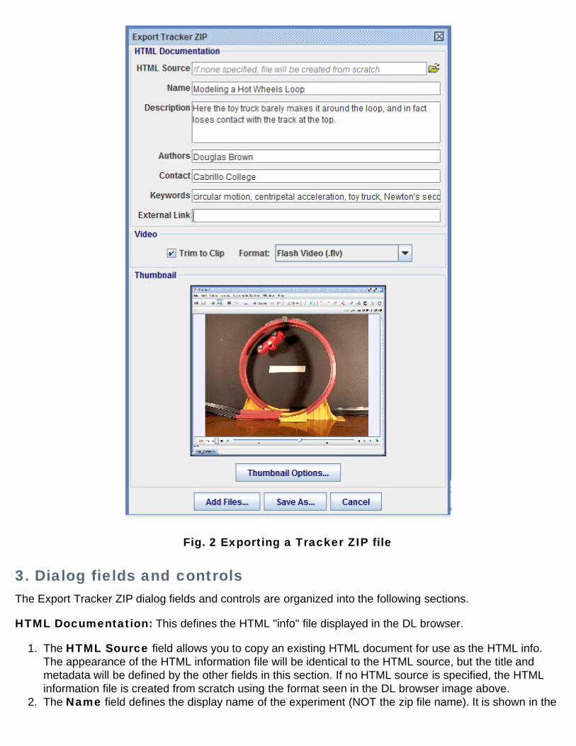
Fig. 2 Exporting a Tracker ZIP file

3. Dialog fields and controlsThe Export Tracker ZIP dialog fields and controls are organized into the following sections.

HTML Documentation: This defines the HTML "info" file displayed in the DL browser.

1. The HTML Source field allows you to copy an existing HTML document for use as the HTML info.The appearance of the HTML information file will be identical to the HTML source, but the title andmetadata will be defined by the other fields in this section. If no HTML source is specified, the HTMLinformation file is created from scratch using the format seen in the DL browser image above.

2. The Name field defines the display name of the experiment (NOT the zip file name). It is shown in the

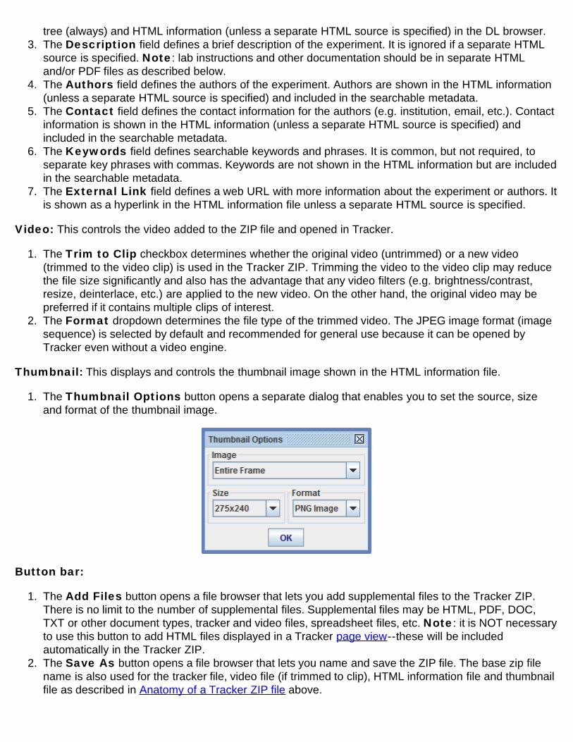
tree (always) and HTML information (unless a separate HTML source is specified) in the DL browser.3. The Description field defines a brief description of the experiment. It is ignored if a separate HTML

source is specified. Note: lab instructions and other documentation should be in separate HTMLand/or PDF files as described below.

4. The Authors field defines the authors of the experiment. Authors are shown in the HTML information(unless a separate HTML source is specified) and included in the searchable metadata.

5. The Contact field defines the contact information for the authors (e.g. institution, email, etc.). Contactinformation is shown in the HTML information (unless a separate HTML source is specified) andincluded in the searchable metadata.

6. The Keywords field defines searchable keywords and phrases. It is common, but not required, toseparate key phrases with commas. Keywords are not shown in the HTML information but are includedin the searchable metadata.

7. The External Link field defines a web URL with more information about the experiment or authors. Itis shown as a hyperlink in the HTML information file unless a separate HTML source is specified.

Video: This controls the video added to the ZIP file and opened in Tracker.

1. The Trim to Clip checkbox determines whether the original video (untrimmed) or a new video(trimmed to the video clip) is used in the Tracker ZIP. Trimming the video to the video clip may reducethe file size significantly and also has the advantage that any video filters (e.g. brightness/contrast,resize, deinterlace, etc.) are applied to the new video. On the other hand, the original video may bepreferred if it contains multiple clips of interest.

2. The Format dropdown determines the file type of the trimmed video. The JPEG image format (imagesequence) is selected by default and recommended for general use because it can be opened byTracker even without a video engine.

Thumbnail: This displays and controls the thumbnail image shown in the HTML information file.

1. The Thumbnail Options button opens a separate dialog that enables you to set the source, sizeand format of the thumbnail image.

Button bar:

1. The Add Files button opens a file browser that lets you add supplemental files to the Tracker ZIP.There is no limit to the number of supplemental files. Supplemental files may be HTML, PDF, DOC,TXT or other document types, tracker and video files, spreadsheet files, etc. Note: it is NOT necessaryto use this button to add HTML files displayed in a Tracker page view--these will be includedautomatically in the Tracker ZIP.

2. The Save As button opens a file browser that lets you name and save the ZIP file. The base zip filename is also used for the tracker file, video file (if trimmed to clip), HTML information file and thumbnailfile as described in Anatomy of a Tracker ZIP file above.

3. The Cancel button closes the dialog. It does not clear the fields, so when you reopen the dalog you donot need to re-enter the information.

4. Sharing Tracker ZIP filesYou can share your Tracker ZIP files directly or on the web.

Direct "live" sharing is perfect for sharing with peers in a classroom or turning in as homework and labreports. It couldn't be much easier:

1. Save the Tracker ZIP file in a shared local directory. All others with access to that directory can openindividual files or the entire directory in the DL browser using the File|Open menu item. Figure 1 at thetop of this page shows what the file "loop2.trz" looks like when open in the DL browser.

2. Email the Tracker ZIP files directly to colleagues or friends. Since they are fully self-contained, copieshave full functionality without requiring links to the original.

Sharing on the web makes your Tracker ZIP experiments available to Tracker users worldwide. Thereare two ways to do this:

1. Create a "live" web collection by uploading the ZIP files to a server along with the OSP DigitalLibrary PHP script. See Digital Library Browser for more information.

2. Use the DL browser to create, edit and upload an XML collection. This gives you the greatestcontrol over the content and organization of your collection. See Digital Library Browser for moreinformation.

To open a web collection in the DL browser, you need to load its URL path (e.g."http://www.my_institution.edu/my_shared_experiments/library_collection.php" or"http://www.my_institution.edu/my_shared_experiments/my_collection.xml"). There are several ways to dothis:

1. Enter the URL path directly into the URL field of the DL browser and click the Load button. See DigitalLibrary Browser for more information.

2. Add the URL path to your personal library ("My Library") and select its menu item in theCollections|My Library menu. See Digital Library Browser for more information.

3. Email the URL path to Douglas Brown (dobrown at cabrillo dot edu) who can (if approved) add it to theCollections|Shared Library menu visible to all Tracker users.

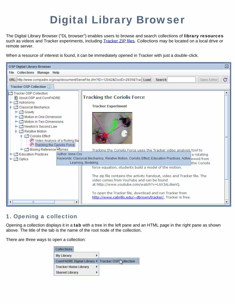
Digital Library BrowserThe Digital Library Browser ("DL browser") enables users to browse and search collections of library resourcessuch as videos and Tracker experiments, including Tracker ZIP files. Collections may be located on a local drive orremote server.

When a resource of interest is found, it can be immediately opened in Tracker with just a double-click.

1. Opening a collectionOpening a collection displays it in a tab with a tree in the left pane and an HTML page in the right pane as shownabove. The title of the tab is the name of the root node of the collection.

There are three ways to open a collection:

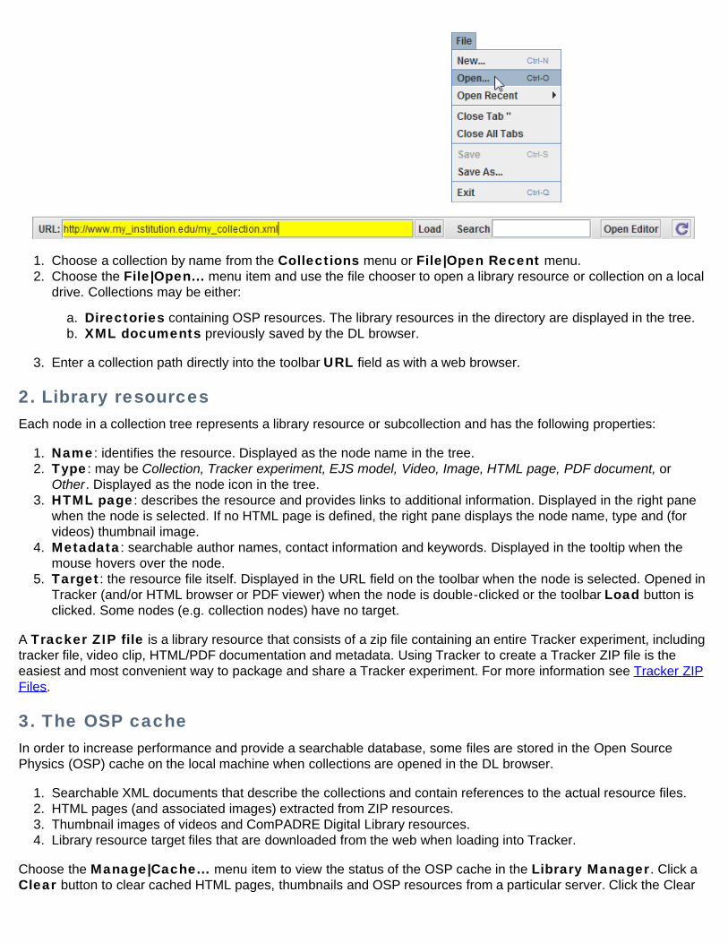
1. Choose a collection by name from the Collections menu or File|Open Recent menu.2. Choose the File|Open... menu item and use the file chooser to open a library resource or collection on a local

drive. Collections may be either:

a. Directories containing OSP resources. The library resources in the directory are displayed in the tree.b. XML documents previously saved by the DL browser.

3. Enter a collection path directly into the toolbar URL field as with a web browser.

2. Library resourcesEach node in a collection tree represents a library resource or subcollection and has the following properties:

1. Name: identifies the resource. Displayed as the node name in the tree.2. Type: may be Collection, Tracker experiment, EJS model, Video, Image, HTML page, PDF document, or

Other. Displayed as the node icon in the tree.3. HTML page: describes the resource and provides links to additional information. Displayed in the right pane

when the node is selected. If no HTML page is defined, the right pane displays the node name, type and (forvideos) thumbnail image.

4. Metadata: searchable author names, contact information and keywords. Displayed in the tooltip when themouse hovers over the node.

5. Target: the resource file itself. Displayed in the URL field on the toolbar when the node is selected. Opened inTracker (and/or HTML browser or PDF viewer) when the node is double-clicked or the toolbar Load button isclicked. Some nodes (e.g. collection nodes) have no target.

A Tracker ZIP file is a library resource that consists of a zip file containing an entire Tracker experiment, includingtracker file, video clip, HTML/PDF documentation and metadata. Using Tracker to create a Tracker ZIP file is theeasiest and most convenient way to package and share a Tracker experiment. For more information see Tracker ZIPFiles.

3. The OSP cacheIn order to increase performance and provide a searchable database, some files are stored in the Open SourcePhysics (OSP) cache on the local machine when collections are opened in the DL browser.

1. Searchable XML documents that describe the collections and contain references to the actual resource files.2. HTML pages (and associated images) extracted from ZIP resources.3. Thumbnail images of videos and ComPADRE Digital Library resources.4. Library resource target files that are downloaded from the web when loading into Tracker.

Choose the Manage|Cache... menu item to view the status of the OSP cache in the Library Manager. Click aClear button to clear cached HTML pages, thumbnails and OSP resources from a particular server. Click the Clear

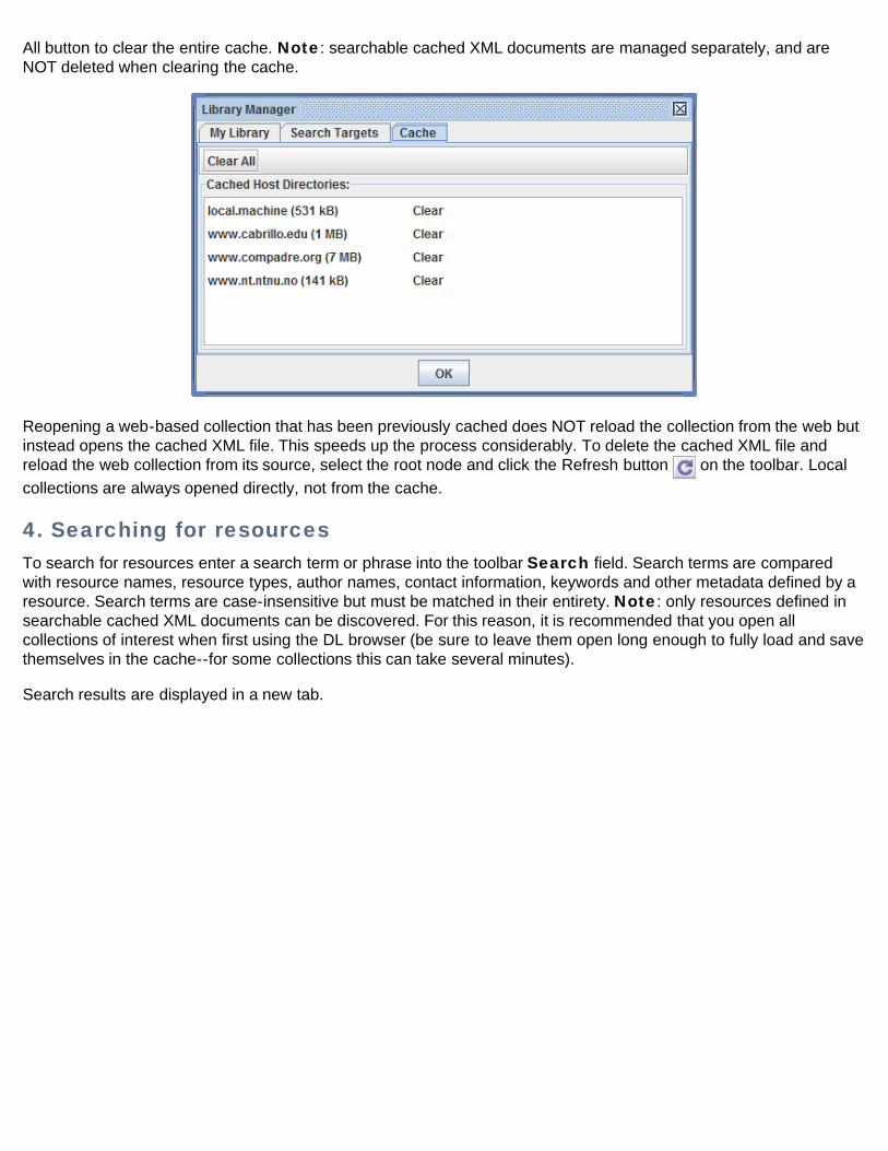
All button to clear the entire cache. Note: searchable cached XML documents are managed separately, and areNOT deleted when clearing the cache.

Reopening a web-based collection that has been previously cached does NOT reload the collection from the web butinstead opens the cached XML file. This speeds up the process considerably. To delete the cached XML file andreload the web collection from its source, select the root node and click the Refresh button on the toolbar. Localcollections are always opened directly, not from the cache.

4. Searching for resourcesTo search for resources enter a search term or phrase into the toolbar Search field. Search terms are comparedwith resource names, resource types, author names, contact information, keywords and other metadata defined by aresource. Search terms are case-insensitive but must be matched in their entirety. Note: only resources defined insearchable cached XML documents can be discovered. For this reason, it is recommended that you open allcollections of interest when first using the DL browser (be sure to leave them open long enough to fully load and savethemselves in the cache--for some collections this can take several minutes).

Search results are displayed in a new tab.

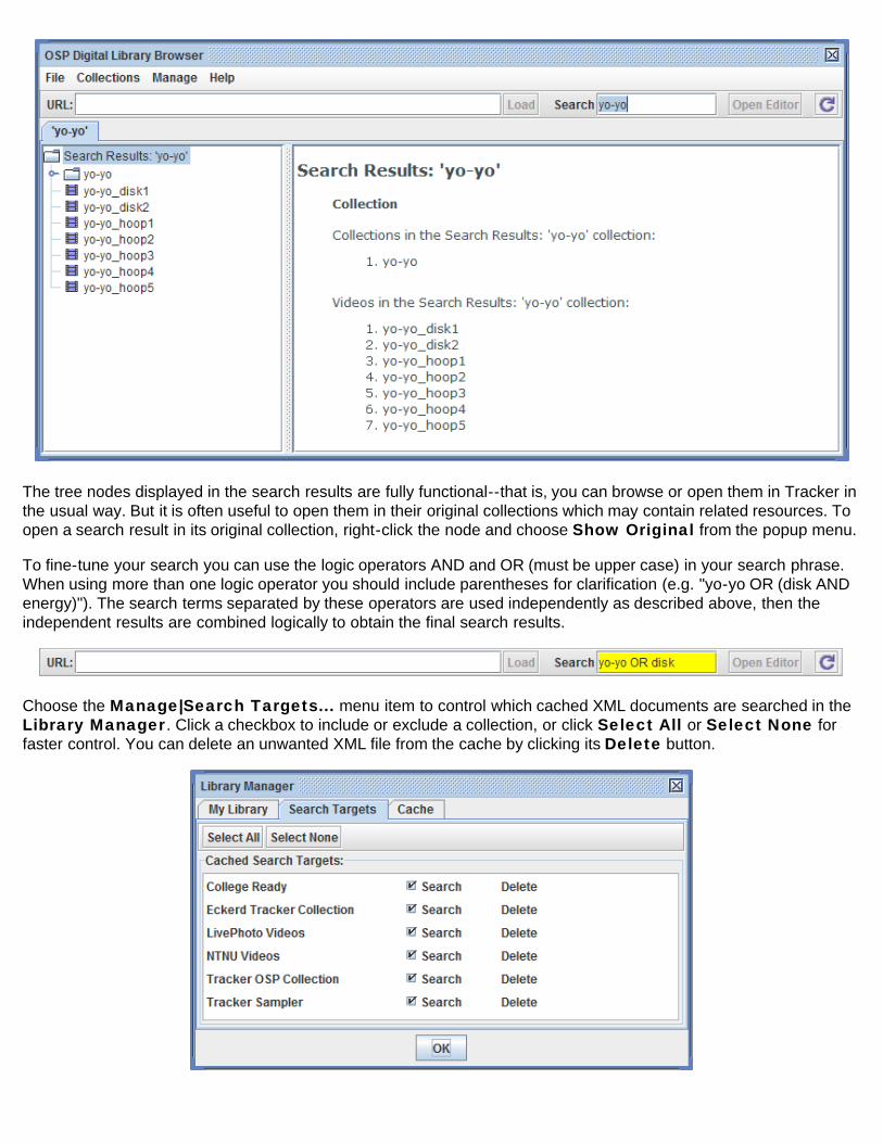
The tree nodes displayed in the search results are fully functional--that is, you can browse or open them in Tracker inthe usual way. But it is often useful to open them in their original collections which may contain related resources. Toopen a search result in its original collection, right-click the node and choose Show Original from the popup menu.

To fine-tune your search you can use the logic operators AND and OR (must be upper case) in your search phrase.When using more than one logic operator you should include parentheses for clarification (e.g. "yo-yo OR (disk ANDenergy)"). The search terms separated by these operators are used independently as described above, then theindependent results are combined logically to obtain the final search results.

Choose the Manage|Search Targets... menu item to control which cached XML documents are searched in theLibrary Manager. Click a checkbox to include or exclude a collection, or click Select All or Select None forfaster control. You can delete an unwanted XML file from the cache by clicking its Delete button.

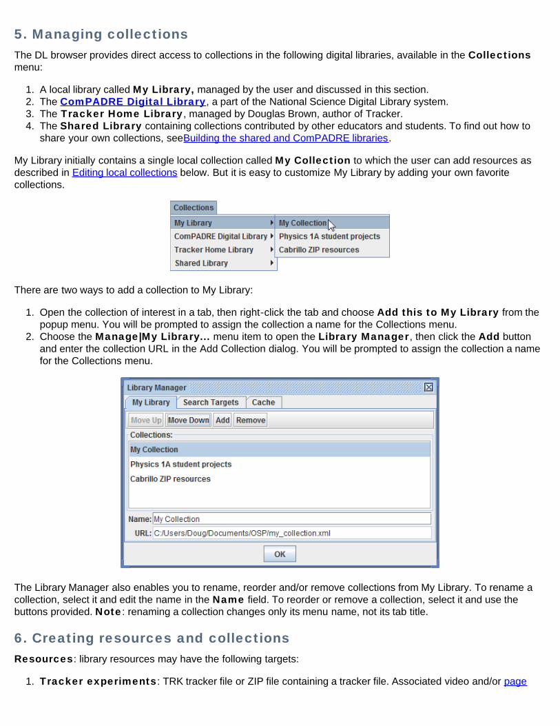
5. Managing collectionsThe DL browser provides direct access to collections in the following digital libraries, available in the Collectionsmenu:

1. A local library called My Library, managed by the user and discussed in this section.2. The ComPADRE Digital Library, a part of the National Science Digital Library system.3. The Tracker Home Library, managed by Douglas Brown, author of Tracker.4. The Shared Library containing collections contributed by other educators and students. To find out how to

share your own collections, seeBuilding the shared and ComPADRE libraries.

My Library initially contains a single local collection called My Collection to which the user can add resources asdescribed in Editing local collections below. But it is easy to customize My Library by adding your own favoritecollections.

There are two ways to add a collection to My Library:

1. Open the collection of interest in a tab, then right-click the tab and choose Add this to My Library from thepopup menu. You will be prompted to assign the collection a name for the Collections menu.

2. Choose the Manage|My Library... menu item to open the Library Manager, then click the Add buttonand enter the collection URL in the Add Collection dialog. You will be prompted to assign the collection a namefor the Collections menu.

The Library Manager also enables you to rename, reorder and/or remove collections from My Library. To rename acollection, select it and edit the name in the Name field. To reorder or remove a collection, select it and use thebuttons provided. Note: renaming a collection changes only its menu name, not its tab title.

6. Creating resources and collectionsResources: library resources may have the following targets:

1. Tracker experiments: TRK tracker file or ZIP file containing a tracker file. Associated video and/or page

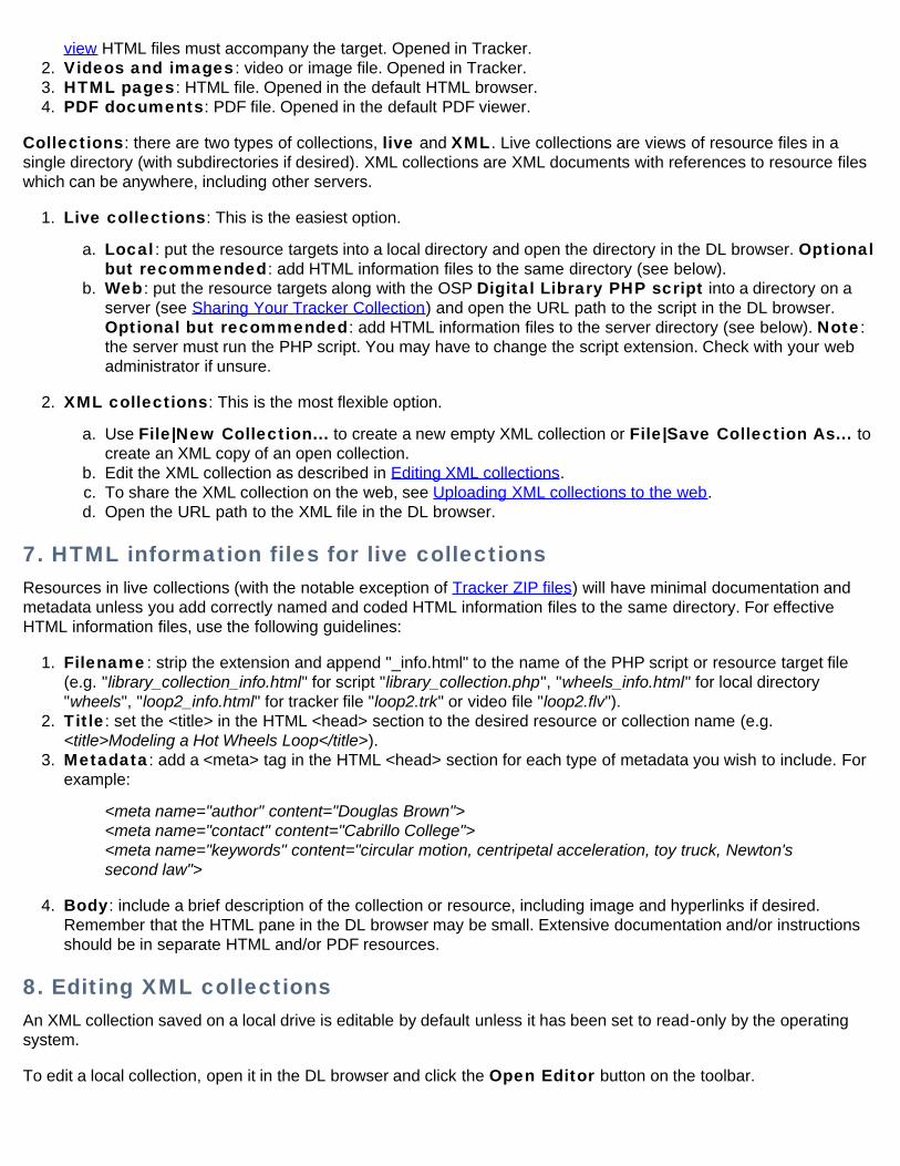
view HTML files must accompany the target. Opened in Tracker.2. Videos and images: video or image file. Opened in Tracker.3. HTML pages: HTML file. Opened in the default HTML browser.4. PDF documents: PDF file. Opened in the default PDF viewer.

Collections: there are two types of collections, live and XML. Live collections are views of resource files in asingle directory (with subdirectories if desired). XML collections are XML documents with references to resource fileswhich can be anywhere, including other servers.

1. Live collections: This is the easiest option.

a. Local: put the resource targets into a local directory and open the directory in the DL browser. Optionalbut recommended: add HTML information files to the same directory (see below).

b. Web: put the resource targets along with the OSP Digital Library PHP script into a directory on aserver (see Sharing Your Tracker Collection) and open the URL path to the script in the DL browser.Optional but recommended: add HTML information files to the server directory (see below). Note:the server must run the PHP script. You may have to change the script extension. Check with your webadministrator if unsure.

2. XML collections: This is the most flexible option.

a. Use File|New Collection... to create a new empty XML collection or File|Save Collection As... tocreate an XML copy of an open collection.

b. Edit the XML collection as described in Editing XML collections.c. To share the XML collection on the web, see Uploading XML collections to the web.d. Open the URL path to the XML file in the DL browser.

7. HTML information files for live collectionsResources in live collections (with the notable exception of Tracker ZIP files) will have minimal documentation andmetadata unless you add correctly named and coded HTML information files to the same directory. For effectiveHTML information files, use the following guidelines:

1. Filename: strip the extension and append "_info.html" to the name of the PHP script or resource target file(e.g. "library_collection_info.html" for script "library_collection.php", "wheels_info.html" for local directory"wheels", "loop2_info.html" for tracker file "loop2.trk" or video file "loop2.flv").

2. Title: set the <title> in the HTML <head> section to the desired resource or collection name (e.g.<title>Modeling a Hot Wheels Loop</title>).

3. Metadata: add a <meta> tag in the HTML <head> section for each type of metadata you wish to include. Forexample:

<meta name="author" content="Douglas Brown"><meta name="contact" content="Cabrillo College"><meta name="keywords" content="circular motion, centripetal acceleration, toy truck, Newton'ssecond law">

4. Body: include a brief description of the collection or resource, including image and hyperlinks if desired.Remember that the HTML pane in the DL browser may be small. Extensive documentation and/or instructionsshould be in separate HTML and/or PDF resources.

8. Editing XML collectionsAn XML collection saved on a local drive is editable by default unless it has been set to read-only by the operatingsystem.

To edit a local collection, open it in the DL browser and click the Open Editor button on the toolbar.

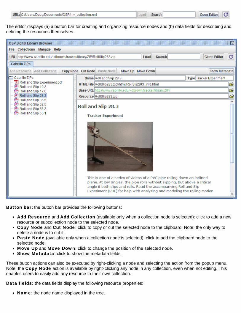
The editor displays (a) a button bar for creating and organizing resource nodes and (b) data fields for describing anddefining the resources themselves.

Button bar: the button bar provides the following buttons:

Add Resource and Add Collection (available only when a collection node is selected): click to add a newresource or subcollection node to the selected node.Copy Node and Cut Node: click to copy or cut the selected node to the clipboard. Note: the only way todelete a node is to cut it.Paste Node (available only when a collection node is selected): click to add the clipboard node to theselected node.Move Up and Move Down: click to change the position of the selected node.Show Metadata: click to show the metadata fields.

These button actions can also be executed by right-clicking a node and selecting the action from the popup menu.Note: the Copy Node action is available by right-clicking any node in any collection, even when not editing. Thisenables users to easily add any resource to their own collection.

Data fields: the data fields display the following resource properties:

Name: the node name displayed in the tree.

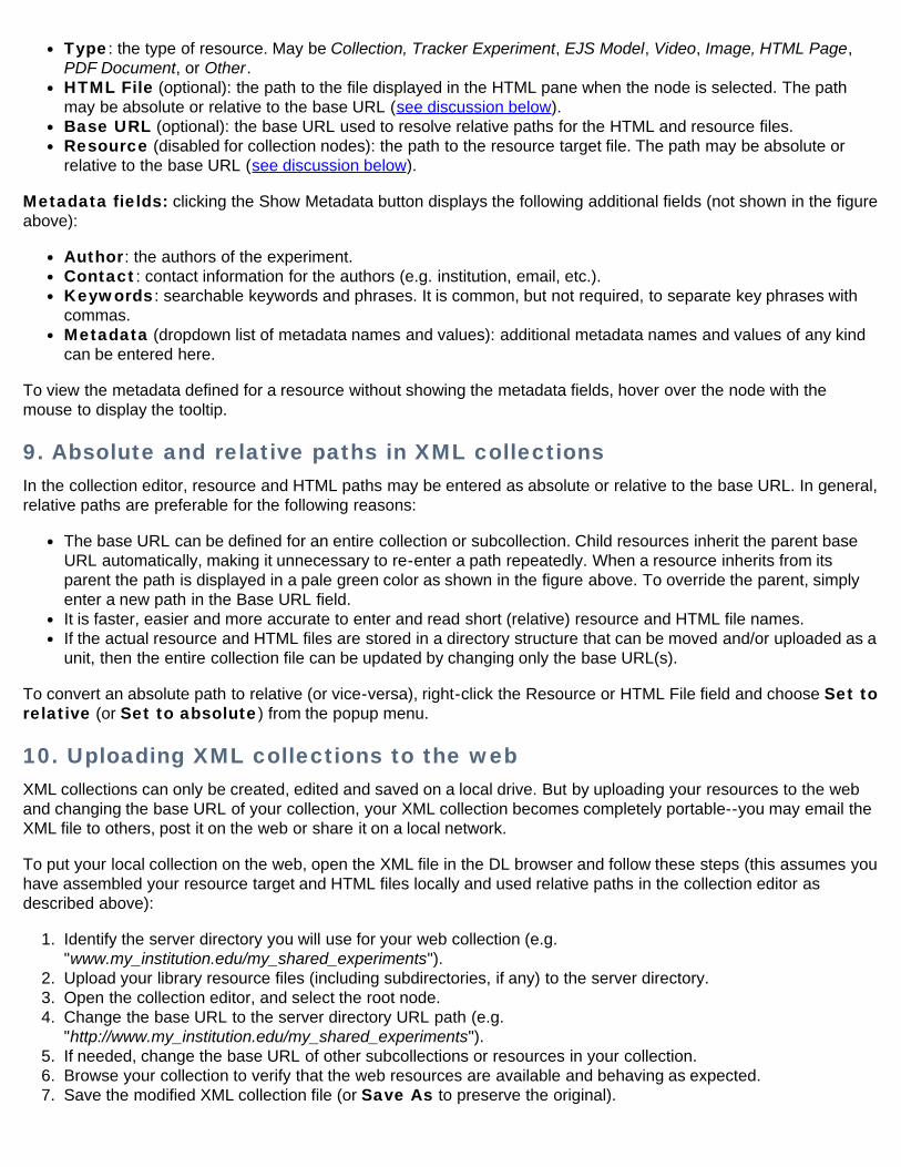
Type: the type of resource. May be Collection, Tracker Experiment, EJS Model, Video, Image, HTML Page,PDF Document, or Other.HTML File (optional): the path to the file displayed in the HTML pane when the node is selected. The pathmay be absolute or relative to the base URL (see discussion below).Base URL (optional): the base URL used to resolve relative paths for the HTML and resource files.Resource (disabled for collection nodes): the path to the resource target file. The path may be absolute orrelative to the base URL (see discussion below).

Metadata fields: clicking the Show Metadata button displays the following additional fields (not shown in the figureabove):

Author: the authors of the experiment.Contact: contact information for the authors (e.g. institution, email, etc.).Keywords: searchable keywords and phrases. It is common, but not required, to separate key phrases withcommas.Metadata (dropdown list of metadata names and values): additional metadata names and values of any kindcan be entered here.

To view the metadata defined for a resource without showing the metadata fields, hover over the node with themouse to display the tooltip.

9. Absolute and relative paths in XML collectionsIn the collection editor, resource and HTML paths may be entered as absolute or relative to the base URL. In general,relative paths are preferable for the following reasons:

The base URL can be defined for an entire collection or subcollection. Child resources inherit the parent baseURL automatically, making it unnecessary to re-enter a path repeatedly. When a resource inherits from itsparent the path is displayed in a pale green color as shown in the figure above. To override the parent, simplyenter a new path in the Base URL field.It is faster, easier and more accurate to enter and read short (relative) resource and HTML file names.If the actual resource and HTML files are stored in a directory structure that can be moved and/or uploaded as aunit, then the entire collection file can be updated by changing only the base URL(s).

To convert an absolute path to relative (or vice-versa), right-click the Resource or HTML File field and choose Set torelative (or Set to absolute) from the popup menu.

10. Uploading XML collections to the webXML collections can only be created, edited and saved on a local drive. But by uploading your resources to the weband changing the base URL of your collection, your XML collection becomes completely portable--you may email theXML file to others, post it on the web or share it on a local network.

To put your local collection on the web, open the XML file in the DL browser and follow these steps (this assumes youhave assembled your resource target and HTML files locally and used relative paths in the collection editor asdescribed above):

1. Identify the server directory you will use for your web collection (e.g."www.my_institution.edu/my_shared_experiments").

2. Upload your library resource files (including subdirectories, if any) to the server directory.3. Open the collection editor, and select the root node.4. Change the base URL to the server directory URL path (e.g.

"http://www.my_institution.edu/my_shared_experiments").5. If needed, change the base URL of other subcollections or resources in your collection.6. Browse your collection to verify that the web resources are available and behaving as expected.7. Save the modified XML collection file (or Save As to preserve the original).

11. Building the Shared and ComPADRE librariesThe Shared Library contains collections contributed by other Tracker users, and we encourage you to help buildthe library by developing and hosting web-based collections (Tracker experiments and/or videos) and emailing thecollection path to the Shared Library editor, Douglas Brown (dobrown at cabrillo dot edu). Collections that are addedto the library are immediately available from the Collections|Shared Library menu visible to all Tracker users.

The ComPADRE Digital Library, a part of the National Science Digital Library system, is a growing network ofeducational resource collections supporting teachers and students in Physics and Astronomy. As a user you mayexplore collections designed to meet your specific needs and help build the network by recommending resources,commenting on resources, and starting or joining discussions. For more information, see<http://www.compadre.org/OSP/>. To recommend an OSP resource for ComPADRE, visit the Suggest aResource page at <http://www.compadre.org/osp/items/suggest.cfm>. Contact the OSP Collection editor,Wolfgang Christian, for additional information.