Embed Size (px)
Citation preview
lable at ScienceDirect
Atmospheric Environment 44 (2010) 204e214
Contents lists avai
Atmospheric Environment
journal homepage: www.elsevier .com/locate/a tmosenv
Tracer studies to characterize the effects of roadside noise barriers on near-roadpollutant dispersion under varying atmospheric stability conditionsq
Dennis Finn a,*, Kirk L. Clawson a, Roger G. Carter a, Jason D. Rich a, Richard M. Eckman a,Steven G. Perry b, Vlad Isakov b, David K. Heist b
aAir Resources Laboratory, Field Research Division, National Oceanic and Atmospheric Administration, 1750 Foote Drive, Idaho Falls, ID 83402, USAbAtmospheric Modeling and Analysis Division, National Exposure Research Laboratory, U.S. Environmental Protection Agency, Research Triangle Park, NC, USA
a r t i c l e i n f o
Article history:Received 12 May 2009Received in revised form25 September 2009Accepted 12 October 2009
Keywords:Wake zoneTraffic emissionsPollutant dispersion near roadwaysConcentration deficits
q Sponsorship: This work was completed under Int92274201-0 between the National Oceanic and Atmthe U.S. Environmental Protection Agency.* Corresponding author. Tel.: þ1 208 526 0566; fax
E-mail address: [email protected] (D. Finn).
1352-2310/$ e see front matter Published by Elsevierdoi:10.1016/j.atmosenv.2009.10.012
a b s t r a c t
A roadway toxics dispersion study was conducted at the Idaho National Laboratory (INL) to document theeffects on concentrations of roadway emissions behind a roadside sound barrier in various conditions ofatmospheric stability. The homogeneous fetch of the INL, controlled emission source, lack of othermanmade or natural flow obstructions, and absence of vehicle-generated turbulence reduced theambiguities in interpretation of the data. Roadway emissions were simulated by the release of anatmospheric tracer (SF6) from two 54 m long line sources, one for an experiment with a 90 m long noisebarrier and one for a control experiment without a barrier. Simultaneous near-surface tracer concen-tration measurements were made with bag samplers on identical sampling grids downwind from theline sources. An array of six 3-d sonic anemometers was employed to measure the barrier-inducedturbulence. Key findings of the study are: (1) the areal extent of higher concentrations and the absolutemagnitudes of the concentrations both increased as atmospheric stability increased; (2) a concentrationdeficit developed in the wake zone of the barrier with respect to concentrations at the same relativelocations on the control experiment at all atmospheric stabilities; (3) lateral dispersion was significantlygreater on the barrier grid than the non-barrier grid; and (4) the barrier tended to trap high concen-trations near the “roadway” (i.e. upwind of the barrier) in low wind speed conditions, especially in stableconditions.
Published by Elsevier Ltd.
1. Introduction
Vehicle-related toxic emissions from roadways include suchpollutants as particulate matter, carbon monoxide, heavy metals,and volatile organic compounds such as benzene. Numerousstudies have found that people living and working near roadwaysare exposed to elevated levels of pollution and are at increased riskof respiratory problems (e.g., Nitta et al., 1993; McConnell et al.,2006), birth and developmental defects (e.g., Wilhelm and Ritz,2003), premature mortality (e.g., Finkelstein et al., 2004; Jerrettet al., 2005), cardiovascular effects (e.g., Peters et al., 2004; Riedikeret al., 2004), and cancer (e.g., Harrison et al., 1999; Pearson et al.,2000). Given that noise barriers and vegetation are now commonroadside features it is pertinent to ask what effect they might haveon pollution levels adjacent to roadways.
eragency Agreement DW-13-ospheric Administration and
: þ1 208 526 2549.
Ltd.
Many studies have looked at the effects of roadside noisebarriers on pollution levels in adjacent areas. Some of these studiessuggest that, for gaseous pollutants, a barrier results in a well-mixed zone with lower concentration extending downwind behindthe barrier (Baldauf et al., 2008; Nokes and Benson, 1984; Paul-Carpenter and Barboza, 1988; H~olscher et al., 1993; Bowker et al.,2007). Depending upon roadway plus barrier configuration,concentration deficits of 50% or more have been observed relativeto a reference roadway configuration without a barrier. Theseconcentration deficit regions can extend in excess of 20 wallheights downwind (Heist et al., 2009). The low concentrationregion has been attributed to upward deflection of the airflow andincreased vertical mixing due to the barrier as well as enhancedinitial mixing due to turbulence on the roadway generated bytraffic. For heavy metals such as lead, a barrier will inhibit down-wind transport and result in increased deposition in the roadwayarea (Swamy and Lokesh, 1993).
Several studies have also examined the role of roadside vegeta-tion (Bowker et al., 2007; Beckett et al., 2000; Bussotti et al., 1995;Heath et al., 1999; Heichel and Hankin, 1976; Munch, 1993; Tan andLepp,1977: Swamyand Lokesh,1993;Madders and Lawrence,1985).

D. Finn et al. / Atmospheric Environment 44 (2010) 204e214 205
These studies suggest that vegetation also reduced downwindpollutant concentrations by enhancing mixing and dispersion aswell as increased the deposition of some species (e.g. heavymetals)in the immediate roadway area.
Despite the accumulating evidence, uncertainties regarding theeffects of roadside noise barriers on pollutant concentrations insurrounding areas remain. Specifically, the role of atmosphericstability has not been investigated in any systematic manner. Mostwind tunnel studies are done in neutral stability conditions andmost of the field experimental work has been done during thedaytime. Furthermore, much of the field work has been done in“natural” settings featuring moving traffic and the associatedturbulence, variations in source strength, and irregular distribu-tions of flow obstructions. All of these can considerably complicatethe interpretation of results.
The Field Research Division (FRD) of the Air Resources Labora-tory (ARL) of the National Oceanic Atmospheric Administration(NOAA) conducted the Near Roadway Tracer Study (NRTS08)during October 2008. The work was sponsored by the AtmosphericModeling and Analysis Division of the U.S. Environmental Protec-tion Agency (EPA). NRTS08 was designed to quantify the effects ofroadside barriers on the downwind dispersion of atmosphericpollutants emitted by roadway sources (e.g. vehicular transport).Pollutant transport and dispersion were measured during the fieldtests using sulfur hexafluoride (SF6) tracer gas as a pollutantsurrogate. The turbulence field driving the dispersion was alsomeasured. The goal of the study was to produce a roadway barrierdata set that (1) covered a range of atmospheric stabilities, (2)minimized factors that could complicate data interpretation, and(3) could be used to guide further development of models such asAERMOD (Cimorelli et al., 2005) to simulate the effects of roadwayemissions.
2. Methods
The field studywas done near NOAA's Grid 3 diffusion grid at theDepartment of Energy's Idaho National Laboratory (INL). The Grid 3area on the INL was selected for NRTS08 for a number of reasons.The INL is located across a broad, relatively flat plain on thewesternedge of the Snake River Plain in southeast Idaho. The Grid 3 areawas originally designed to conduct transport and dispersion tracerstudies in the 1950s. It is part of the INL mesonet (Clawson et al.,2007). Numerous tracer and other atmospheric studies have beenconducted at Grid 3 since that time (Start et al., 1984; Sagendorf andDickson, 1974; Garodz and Clawson, 1991, 1993). ConductingNRTS08 at Grid 3 allowed for optimal control of the experimentalconfiguration, in particular, the need for having the roadway andbarrier oriented perpendicular to the wind direction. This controlincreased the chances of obtaining high quality measurements thatwould be of the greatest benefit toward the goal of improvingmodel reliability. The general selection of the site and timing for theexperiments were also guided by historical wind rose data gener-ated by the NOAA-INLmesonet to afford themaximum opportunityfor the realization of ideal wind direction conditions. The open,level terrain without other manmade or natural obstructions orcomplexities also made the data easier to interpret.
Five tests were conducted during NRTS08, each spanning a 3-hperiod broken into 15-min tracer sampling intervals. One test wasconducted in unstable conditions, one in neutral conditions, andthree in stable conditions. All lengths and distances in the studywere referenced to multiples of the barrier height H. A 90 m long(15H) by 6 m high (1H ¼ 6 m) straw bale stack representeda roadway barrier for the primary experiment (Fig. 1). The“roadway” itself was nothingmore than an access track through thesagebrush adjacent to the barrier. The primary and reference
control experiments both had a 54 m long (9H) SF6 tracer linesource release positioned 1 m above ground level (AGL) repre-senting pollution sources from a roadway on the upwind side of thebarrier and a gridded array of bag samplers downwind of the linesource and barrier for measuring mean 15-min concentrations(Fig. 2). An array of six 3-d sonic anemometers was deployed formaking wind and turbulence measurements, 5 on the primaryexperiment and 1 on the control experiment (Fig. 3). The barrierwas oriented at 303� azimuth in order to be approximatelyperpendicular to the prevailing SSW winds during the day and NEdrainage flows at night. It was located 1H downwind of the linesource so that the source represented the median for a virtual 2-lane roadway 2H in width, including shoulders. The barrier was36 m longer than the line source in an attempt to minimize barrieredge effects, i.e., tracer leaking around the barrier.
The primary and control experimental sampling grids hada large crosswind separation of about 700 m at the point of closestproximity between the edges of the two grids to eliminate possibleinterferences. Each sampling grid was composed of two sub-grids,one NE of the release line and one SW of the release line. The NEsub-grid was used for SW winds and the SW sub-grid was used forNE winds. The origin for the grid coordinate system was themidpoint of the line source release with x positive in the stream-wise direction, perpendicular to the barrier, the y-axis was alongthe line source, and the positive z-directionwas vertically upwards.
The location of the sonic anemometers was governed by: (1) theneed to measure the upwind approach flow, (2) the need tomeasure the turbulence field as close as practical to the line source,and (3) the importance of measuring the turbulence field in thewake region of the barrier where the greatest changes in theconcentration and turbulence fields were expected to occur. Oneanemometer was located �1.6H upwind of the line source on thecontrol experiment at a height of 3 m (0.5H) and served asa reference for the approach flow. Another anemometer waslocated�1.6H upwind of the line source on the primary experimentat a height of 0.5H for measuring turbulence in the tracer releasearea and the effects of the barrier on the approach flow. Threeanemometers were located on a tower 4H downwind of the releaseat heights of 3, 6, and 9 m (0.5, 1, 1.5H, respectively) to providea vertical profile of the flow and turbulence through and above thebarrier wake region. A fourth was located farther downwind at 11Hnear the estimated flow reattachment zone. Five of the sonics wereR.M. Young Model 81000 Ultrasonic Anemometers and one wasa Gill Windmaster Pro Anemometer. An additional suite ofsupplemental meteorological measurements were made on the INLmesonet and at a 30 m tower located between the two grids(Clawson et al., 2009).
Each of the two sampling grids had 58 sampler locationsmarkedby metal fence posts. The design of the grids was patterned afterthe work of Heist et al. (2009), to provide a basis for intercompar-ison of near-neutral data, and guided by considerations of wherethe greatest changes in the concentration field were expected. Heistet al. (2009) indicated that the largest alongwind concentrationgradients and greatest differences between the barrier and flatterrain cases in wind tunnel studies occurred within the first10e15H. For this reason, sampler density was greatest near thebarrier and decreased in the downwind direction (Fig. 2). Two ofthe samplers were deployed upwind of the release line at x ¼ �1Hand x¼�2H to check for possible upwind tracer dispersion. All bagsamplers were attached to the metal fence posts at approximately1.5 m AGL. In addition to the 58 regular samplers on each grid, anadditional 9 samplers were deployed for quality control purposes.These included field duplicates, field controls, and field blanks.
The SF6 bag samplers housed a microprocessor and 12 micro-processor-controlled air pumps designed to sequentially fill sample

Fig. 1. Mock straw bale sound barrier, 6 m high and 90 m long.
D. Finn et al. / Atmospheric Environment 44 (2010) 204e214206
bags for a specified time and duration. Sampler cartridges loadedwith 12 Tedlar� bags were installed in the samplers and each bagwas filled for 15 min. Bag samples were analyzed using gas chro-matography at the FRD Tracer Analysis Facility in Idaho Falls, Idaho.
-18.0
-13.5
-9.0
-4.5
0.0
4.5
9.0
13.5
18.0
y (H
)
302520151050-5x (H)
Fig. 2. Schematic map of the primary sampling grid with locations of the anemome-ters (�), line source release (solid line), barrier (bold line), and tracer samplers (C).The anemometer indicated at x ¼ 4H represents a tower with anemometers at z ¼ 3, 6,and 9 m.
A complete description of the analytical procedures and rigorousquality control procedures used are described in Clawson et al.(2005, 2009). The data reported are accurate to within �20% ofNIST-certified standards and, with very few exceptions, are accu-rate within �10%.
A single tracer line source was used to simulate roadwayemissions for the primary and control experimental grids. Thetracer release systemwas engineered to simultaneously release SF6from two independently controlled release systems and dissemi-nation lines, one for each grid (Fig. 4). This permitted measurementof barrier and non-barrier dispersion effects under identicalmeteorological conditions. During tracer releases, gaseous SF6tracer flowed from small (about 8 kg) aluminum cylinders con-taining liquid SF6, through calibrated mass flow controllers, andinto flexible 0.125 inch (3.175 mm) inside diameter polyurethanetubes connected to the two 54 m long release lines. The flowcontrollers provided temporal flow consistency of better than 1%over the duration of each release period. The absolute accuracy ofthe mass flow controllers was�2% of full scale. Uniform flow acrossthe line was assured by maintaining equal pressure drop at each of64 equally spaced release points on each line. The release pointswere 31-gage hypodermic needles. Equal pressure drop wasmaintained by supplying tracer gas using a 6-level binary networkand equal lengths of tubing to divide the flow to each of the nee-dles. Rotameter flow measurements at each needle confirmeduniform flow across each line within �10% prior to each test.
The mass flow controller measurements of SF6 were checkedagainst the total mass released. The total mass of SF6 released foreach test on the two release lines was determined using thebeginning and ending weight of the SF6 cylinders as measured bya precision Ohaus AV8101 electronic scale for each of the twobottles. These scales were capable of weighing up to 8100 g witha resolution of 0.1 g and a full range accuracy of 0.4 g. The scalecalibration was checked prior to each release. Knownweights wereplaced on the scale along with the SF6 cylinder still attached. It wasfound that the scale was within the 0.4 g manufacturer

Fig. 3. Photo of bag samplers and anemometers at x ¼ 4H (tower) and 11H downwind of the barrier.
D. Finn et al. / Atmospheric Environment 44 (2010) 204e214 207
specification on all tests. With the overall accuracy of the scalebeing 0.4 g and the smallest total release during a test being 269 gof SF6, the maximum uncertainty of SF6 released during a test wasless than 0.15 percent. Additional details on the line source areprovided in Clawson et al. (2009).
Fig. 4. Diagram of the S
The SF6 tracer was simultaneously released from the line sourcefor each grid beginning 15 min before the sampler measurementsstarted to establish a quasi-steady state concentration field andcontinued until the end of each test. Tracer release rates rangedfrom 0.02 to 0.05 g s�1.
F6 release system.
D. Finn et al. / Atmospheric Environment 44 (2010) 204e214208
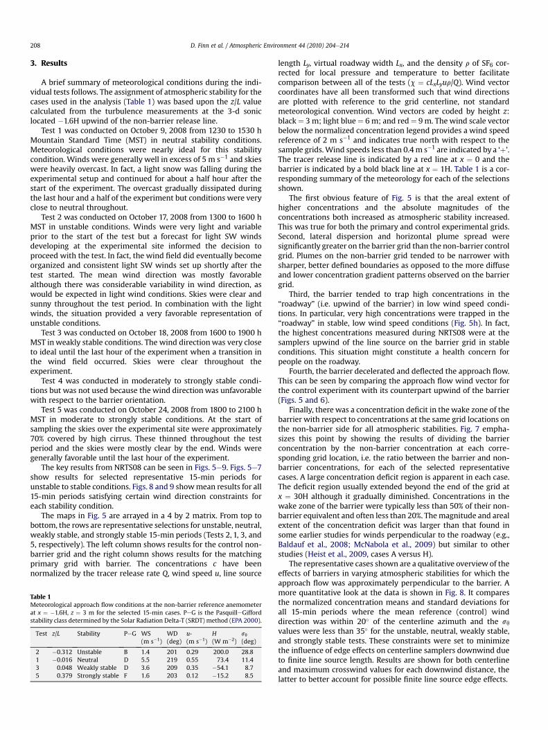
3. Results
A brief summary of meteorological conditions during the indi-vidual tests follows. The assignment of atmospheric stability for thecases used in the analysis (Table 1) was based upon the z/L valuecalculated from the turbulence measurements at the 3-d soniclocated �1.6H upwind of the non-barrier release line.
Test 1 was conducted on October 9, 2008 from 1230 to 1530 hMountain Standard Time (MST) in neutral stability conditions.Meteorological conditions were nearly ideal for this stabilitycondition. Winds were generally well in excess of 5 m s�1 and skieswere heavily overcast. In fact, a light snow was falling during theexperimental setup and continued for about a half hour after thestart of the experiment. The overcast gradually dissipated duringthe last hour and a half of the experiment but conditions were veryclose to neutral throughout.
Test 2 was conducted on October 17, 2008 from 1300 to 1600 hMST in unstable conditions. Winds were very light and variableprior to the start of the test but a forecast for light SW windsdeveloping at the experimental site informed the decision toproceed with the test. In fact, the wind field did eventually becomeorganized and consistent light SW winds set up shortly after thetest started. The mean wind direction was mostly favorablealthough there was considerable variability in wind direction, aswould be expected in light wind conditions. Skies were clear andsunny throughout the test period. In combination with the lightwinds, the situation provided a very favorable representation ofunstable conditions.
Test 3 was conducted on October 18, 2008 from 1600 to 1900 hMST inweakly stable conditions. The wind directionwas very closeto ideal until the last hour of the experiment when a transition inthe wind field occurred. Skies were clear throughout theexperiment.
Test 4 was conducted in moderately to strongly stable condi-tions but was not used because the wind direction was unfavorablewith respect to the barrier orientation.
Test 5 was conducted on October 24, 2008 from 1800 to 2100 hMST in moderate to strongly stable conditions. At the start ofsampling the skies over the experimental site were approximately70% covered by high cirrus. These thinned throughout the testperiod and the skies were mostly clear by the end. Winds weregenerally favorable until the last hour of the experiment.
The key results from NRTS08 can be seen in Figs. 5e9. Figs. 5e7show results for selected representative 15-min periods forunstable to stable conditions. Figs. 8 and 9 showmean results for all15-min periods satisfying certain wind direction constraints foreach stability condition.
The maps in Fig. 5 are arrayed in a 4 by 2 matrix. From top tobottom, the rows are representative selections for unstable, neutral,weakly stable, and strongly stable 15-min periods (Tests 2, 1, 3, and5, respectively). The left column shows results for the control non-barrier grid and the right column shows results for the matchingprimary grid with barrier. The concentrations c have beennormalized by the tracer release rate Q, wind speed u, line source
Table 1Meteorological approach flow conditions at the non-barrier reference anemometerat x ¼ �1.6H, z ¼ 3 m for the selected 15-min cases. PeG is the PasquilleGiffordstability class determined by the Solar Radiation Delta-T (SRDT) method (EPA 2000).
Test z/L Stability PeG WS(m s�1)
WD(deg)
u*(m s�1)
H(W m�2)
sq(deg)
2 �0.312 Unstable B 1.4 201 0.29 200.0 28.81 �0.016 Neutral D 5.5 219 0.55 73.4 11.43 0.048 Weakly stable D 3.6 209 0.35 �54.1 8.75 0.379 Strongly stable F 1.6 203 0.12 �15.2 8.5
length Ly, virtual roadway width Lx, and the density r of SF6 cor-rected for local pressure and temperature to better facilitatecomparison between all of the tests (c ¼ cLxLyur/Q). Wind vectorcoordinates have all been transformed such that wind directionsare plotted with reference to the grid centerline, not standardmeteorological convention. Wind vectors are coded by height z:black¼ 3 m; light blue¼ 6 m; and red¼ 9m. The wind scale vectorbelow the normalized concentration legend provides a wind speedreference of 2 m s�1 and indicates true north with respect to thesample grids.Wind speeds less than 0.4m s�1 are indicated by a ‘þ’.The tracer release line is indicated by a red line at x ¼ 0 and thebarrier is indicated by a bold black line at x ¼ 1H. Table 1 is a cor-responding summary of the meteorology for each of the selectionsshown.
The first obvious feature of Fig. 5 is that the areal extent ofhigher concentrations and the absolute magnitudes of theconcentrations both increased as atmospheric stability increased.This was true for both the primary and control experimental grids.Second, lateral dispersion and horizontal plume spread weresignificantly greater on the barrier grid than the non-barrier controlgrid. Plumes on the non-barrier grid tended to be narrower withsharper, better defined boundaries as opposed to the more diffuseand lower concentration gradient patterns observed on the barriergrid.
Third, the barrier tended to trap high concentrations in the“roadway” (i.e. upwind of the barrier) in low wind speed condi-tions. In particular, very high concentrations were trapped in the“roadway” in stable, low wind speed conditions (Fig. 5h). In fact,the highest concentrations measured during NRTS08 were at thesamplers upwind of the line source on the barrier grid in stableconditions. This situation might constitute a health concern forpeople on the roadway.
Fourth, the barrier decelerated and deflected the approach flow.This can be seen by comparing the approach flow wind vector forthe control experiment with its counterpart upwind of the barrier(Figs. 5 and 6).
Finally, there was a concentration deficit in the wake zone of thebarrier with respect to concentrations at the same grid locations onthe non-barrier side for all atmospheric stabilities. Fig. 7 empha-sizes this point by showing the results of dividing the barrierconcentration by the non-barrier concentration at each corre-sponding grid location, i.e. the ratio between the barrier and non-barrier concentrations, for each of the selected representativecases. A large concentration deficit region is apparent in each case.The deficit region usually extended beyond the end of the grid atx ¼ 30H although it gradually diminished. Concentrations in thewake zone of the barrier were typically less than 50% of their non-barrier equivalent and often less than 20%. Themagnitude and arealextent of the concentration deficit was larger than that found insome earlier studies for winds perpendicular to the roadway (e.g.,Baldauf et al., 2008; McNabola et al., 2009) but similar to otherstudies (Heist et al., 2009, cases A versus H).
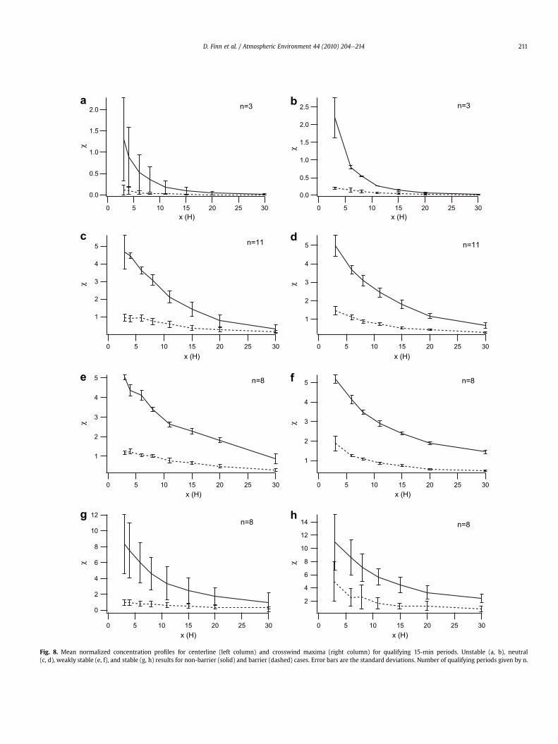
The representative cases shown are a qualitative overview of theeffects of barriers in varying atmospheric stabilities for which theapproach flow was approximately perpendicular to the barrier. Amore quantitative look at the data is shown in Fig. 8. It comparesthe normalized concentration means and standard deviations forall 15-min periods where the mean reference (control) winddirection was within 20� of the centerline azimuth and the sqvalues were less than 35� for the unstable, neutral, weakly stable,and strongly stable tests. These constraints were set to minimizethe influence of edge effects on centerline samplers downwind dueto finite line source length. Results are shown for both centerlineand maximum crosswind values for each downwind distance, thelatter to better account for possible finite line source edge effects.

-18.0
-13.5
-9.0
-4.5
0.0
4.5
9.0
13.5
18.0
Y (H
)
3020100X (H)
h
-18.0
-13.5
-9.0
-4.5
0.0
4.5
9.0
13.5
18.0
Y (H
)
3020100X (H)
g
-18.0
-13.5
-9.0
-4.5
0.0
4.5
9.0
13.5
18.0
(Y (H
)
3020100X (H)
f
-18.0
-13.5
-9.0
-4.5
0.0
4.5
9.0
13.5
18.0
Y (H
)
3020100X (H)
e
-18.0
-13.5
-9.0
-4.5
0.0
4.5
9.0
13.5
18.0
Y (H
)
3020100X (H)
d
-18.0
-13.5
-9.0
-4.5
0.0
4.5
9.0
13.5
18.0
Y (H
)
3020100X (H)
c
-18.0
-13.5
-9.0
-4.5
0.0
4.5
9.0
13.5
18.0
Y (H
)
3020100X (H)
b
-18.0
-13.5
-9.0
-4.5
0.0
4.5
9.0
13.5
18.0
)H( Y
3020100X (H)
a
elbatsnU
Neu
tral
Wea
kly
Stab
leSt
able
(a) unstable, non-barrier(b) unstable, barrier(c) neutral, non-barrier(d) neutral, barrier(e) weakly stable, non-barrier(f) weakly stable, barrier(g) stable, non-barrier(h) stable, barrier
<1e-2
1e-2 to 5e-2
5e-2 to 1e-1
1e-1 to 3e-1
3e-1 to 5e-1
5e-1 to 1e0
1e0 to 5e0
>5e0
N
2 m/s
Fig. 5. Corresponding non-barrier (left column) and barrier (right column) normalized tracer concentration/wind vector maps for representative (a, b) unstable, (c, d) neutral,(e, f) weakly stable, and (g, h) stable cases. Tracer release line is shown in bright red; the barrier in bold black. Wind vector heights are color coded as described in text.(For interpretation of the references to color in this figure legend, the reader is referred to the web version of this article.)
D. Finn et al. / Atmospheric Environment 44 (2010) 204e214 209

10
8
6
4
2
0
z (m
)
0.40.30.20.10.0TKE/u2
6543210
TKE
10
8
6
4
2
0
z (m
)
0.40.30.20.10.0TKE/u2
6543210
TKE10
8
6
4
2
0
z (m
)
0.40.30.20.10.0TKE/u2
6543210
TKE
10
8
6
4
2
0
z (m
)
6420-2x (H)
10
8
6
4
2
0
z (m
)
6420-2x (H)
10
8
6
4
2
0
z (m
)
6420-2x (H)
N10
8
6
4
2
0
z (m
)
6420-2x (H)
a b c d
e f g 10
8
6
4
2
0
z (m
)
0.40.30.20.10.0TKE/u2
6543210
TKEh
Fig. 6. Wind vector and turbulence profile plots for the selected 15-min periods. Profiles for TKE (dashed) and normalized TKE (solid) are shown for the tower at x ¼ 4H. Unstable(a, b); neutral (c, d); weakly stable (e, f); and stable (g, h). The reference north arrow (N) wind vector in (a) has magnitude of 3 m s�1. The ‘þ’ denotes less than 0.4 m s�1. Bold windvector represents the reference wind from the control experiment.
-15
-10
-5
0
5
10
15
Y (H
)
302520151050X (H)
01
10
10
5
5
5
2
2
2
2
1
1 0.7
0.7 0.4
0.4
0.4
0.4
0.2
0.2
0.2
d
-15
-10
-5
0
5
10
15
Y (H
)
302520151050X (H)
10 10
10
10
5 5
5
5
5 2
2 2
2 2
2 2
1
1 1
1 1 1
1 1
1
1 1
0.7 0.7
0.7 0.4
0.4
c
-15
-10
-5
0
5
10
15
Y (H
)
302520151050X (H)
10
10 5
5
5
2
2
2
2
1 1
1
0.7
0.7
0.7
0.7
0.4 0.4
0.4
b
-15
-10
-5
0
5
10
15
Y (H
)
302520151050X (H)
10 5
2 1
0.7 0.7
0.7
0.4
0.4
0.4 0.2 0.2
0.2
0.2 0.2
a
Fig. 7. Contour maps of the ratio between barrier and non-barrier tracer concentrations at corresponding grid locations for the selected (a) unstable, (b) neutral, (c) weakly stable,and (d) stable cases. Tracer release line (bright red) and barrier (bold black) are shown for reference.
12
10
8
6
4
2
0
χ
302520151050x (H)
n=8
5
4
3
2
1
χ
302520151050x (H)
n=8
5
4
3
2
1
χ
302520151050x (H)
n=11
2.0
1.5
1.0
0.5
0.0
χ
302520151050x (H)
n=3
14
12
10
8
6
4
2
χ
302520151050x (H)
n=8
5
4
3
2
1
χ
302520151050x (H)
n=8
5
4
3
2
1
χ
302520151050x (H)
n=11
2.5
2.0
1.5
1.0
0.5
0.0
χ
302520151050x (H)
n=3a b
c d
e f
g h
Fig. 8. Mean normalized concentration profiles for centerline (left column) and crosswind maxima (right column) for qualifying 15-min periods. Unstable (a, b), neutral(c, d), weakly stable (e, f), and stable (g, h) results for non-barrier (solid) and barrier (dashed) cases. Error bars are the standard deviations. Number of qualifying periods given by n.
D. Finn et al. / Atmospheric Environment 44 (2010) 204e214 211
1.4
1.2
1.0
0.8
0.6
0.4
0.2
0.0
-0.2
Rat
io B
arrie
r/No
Barri
er
30252015105x (H)
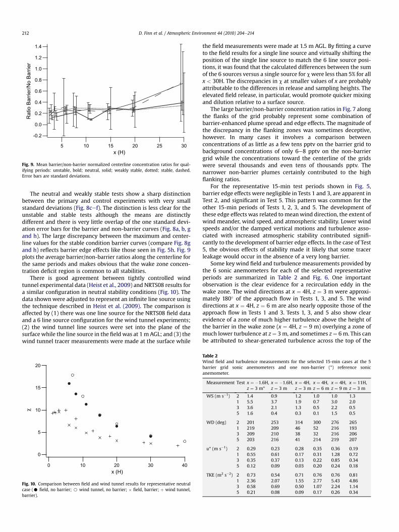
Fig. 9. Mean barrier/non-barrier normalized centerline concentration ratios for qual-ifying periods: unstable, bold; neutral, solid; weakly stable, dotted; stable, dashed.Error bars are standard deviations.
D. Finn et al. / Atmospheric Environment 44 (2010) 204e214212
The neutral and weakly stable tests show a sharp distinctionbetween the primary and control experiments with very smallstandard deviations (Fig. 8cef). The distinction is less clear for theunstable and stable tests although the means are distinctlydifferent and there is very little overlap of the one standard devi-ation error bars for the barrier and non-barrier curves (Fig. 8a, b, gand h). The large discrepancy between the maximum and center-line values for the stable condition barrier curves (compare Fig. 8gand h) reflects barrier edge effects like those seen in Fig. 5h. Fig. 9plots the average barrier/non-barrier ratios along the centerline forthe same periods and makes obvious that the wake zone concen-tration deficit region is common to all stabilities.
There is good agreement between tightly controlled windtunnel experimental data (Heist et al., 2009) and NRTS08 results fora similar configuration in neutral stability conditions (Fig. 10). Thedata shownwere adjusted to represent an infinite line source usingthe technique described in Heist et al. (2009). The comparison isaffected by (1) there was one line source for the NRTS08 field dataand a 6 line source configuration for the wind tunnel experiments;(2) the wind tunnel line sources were set into the plane of thesurfacewhile the line source in the field was at 1m AGL; and (3) thewind tunnel tracer measurements were made at the surface while
20
15
10
5
0
χ
403020100x (H)
Fig. 10. Comparison between field and wind tunnel results for representative neutralcase (C field, no barrier; B wind tunnel, no barrier; � field, barrier; þ wind tunnel,barrier).
the field measurements were made at 1.5 m AGL. By fitting a curveto the field results for a single line source and virtually shifting theposition of the single line source to match the 6 line source posi-tions, it was found that the calculated differences between the sumof the 6 sources versus a single source for cwere less than 5% for allx < 30H. The discrepancies in c at smaller values of x are probablyattributable to the differences in release and sampling heights. Theelevated field release, in particular, would promote quicker mixingand dilution relative to a surface source.
The large barrier/non-barrier concentration ratios in Fig. 7 alongthe flanks of the grid probably represent some combination ofbarrier-enhanced plume spread and edge effects. The magnitude ofthe discrepancy in the flanking zones was sometimes deceptive,however. In many cases it involves a comparison betweenconcentrations of as little as a few tens pptv on the barrier grid tobackground concentrations of only 6e8 pptv on the non-barriergrid while the concentrations toward the centerline of the gridswere several thousands and even tens of thousands pptv. Thenarrower non-barrier plumes certainly contributed to the highflanking ratios.
For the representative 15-min test periods shown in Fig. 5,barrier edge effects were negligible in Tests 1 and 3, are apparent inTest 2, and significant in Test 5. This pattern was common for theother 15-min periods of Tests 1, 2, 3, and 5. The development ofthese edge effects was related to meanwind direction, the extent ofwind meander, wind speed, and atmospheric stability. Lower windspeeds and/or the damped vertical motions and turbulence asso-ciated with increased atmospheric stability contributed signifi-cantly to the development of barrier edge effects. In the case of Test5, the obvious effects of stability made it likely that some tracerleakage would occur in the absence of a very long barrier.
Some key wind field and turbulence measurements provided bythe 6 sonic anemometers for each of the selected representativeperiods are summarized in Table 2 and Fig. 6. One importantobservation is the clear evidence for a recirculation eddy in thewake zone. The wind directions at x ¼ 4H, z ¼ 3 m were approxi-mately 180� of the approach flow in Tests 1, 3, and 5. The winddirections at x ¼ 4H, z ¼ 6 m are also nearly opposite those of theapproach flow in Tests 1 and 3. Tests 1, 3, and 5 also show clearevidence of a zone of much higher turbulence above the height ofthe barrier in the wake zone (x ¼ 4H, z ¼ 9 m) overlying a zone ofmuch lower turbulence at z¼ 3m, and sometimes z¼ 6m. This canbe attributed to shear-generated turbulence across the top of the
Table 2Wind field and turbulence measurements for the selected 15-min cases at the 5barrier grid sonic anemometers and one non-barrier (*) reference sonicanemometer.
Measurement Test x ¼ �1.6H,z ¼ 3 m*
x ¼ �1.6H,z ¼ 3 m
x ¼ 4H,z ¼ 3 m
x ¼ 4H,z ¼ 6 m
x ¼ 4H,z ¼ 9 m
x ¼ 11H,z ¼ 3 m
WS (m s�1) 2 1.4 0.9 1.2 1.0 1.0 1.31 5.5 3.7 1.9 0.7 3.0 2.03 3.6 2.1 1.3 0.5 2.2 0.55 1.6 0.4 0.3 0.1 1.5 0.5
WD (deg) 2 201 253 314 300 276 2651 219 209 46 52 216 1933 209 210 38 32 216 2065 203 216 41 214 219 207
u* (m s�1) 2 0.29 0.23 0.28 0.35 0.36 0.191 0.55 0.61 0.17 0.31 1.28 0.723 0.35 0.37 0.13 0.22 0.85 0.345 0.12 0.09 0.03 0.20 0.24 0.18
TKE (m2 s�2) 2 0.73 0.54 0.71 0.76 0.76 0.811 2.36 2.07 1.55 2.77 5.43 4.863 0.58 0.69 0.50 1.07 2.24 1.145 0.21 0.08 0.09 0.17 0.26 0.34
D. Finn et al. / Atmospheric Environment 44 (2010) 204e214 213
barrier. Finally, the evidence is somewhat mixed on whetherx ¼ 11H was far enough downwind to be beyond the reattachmentpoint of the flow. It appears as if the flow had not fully re-equili-brated with the approach flow in most respects at this distancedownwind. This was expressed by the lower wind speeds and/orturning of the wind vector often observed there relative to thereference anemometer. Again, while there is considerable vari-ability between 15-min periods within a test, the observationsrepresented by the selected cases are common in the data set asa whole.
Test 2, the unstable case, had the least well-defined, shear-generated, high turbulence zone although it had the highestnormalized TKE (Fig. 6). Thewind and turbulence fields appeared tobe more homogeneous than in the other tests. The recirculationeddy was also less well-defined with the wind direction often moreturned at a sharp angle rather than being completely 180� reversed.
The simplest explanations for the observed concentrationpatterns are that (1) the tracer plume was forced to move up andover the barrier, enhancing plume dispersion in the vertical andlowering concentrations behind the barrier; and (2) the plume wasforced to spread horizontally when the approach flow was decel-erated and deflected by the barrier. The former would have had theadditional effect of creating an elevated source. Once the tracerplume was lifted to the top of the barrier, its dispersion would befurther enhanced in a highly turbulent shear zone, furtherdecreasing downwind concentrations.
In low wind speed conditions, it was common for the tracer tobe at least partly impounded and trapped in a low wind speedregion in front of the barrier. Once trapped, turbulent diffusionoften transported some of the tracer back to the samplers upwindof the line source. This effect was exaggerated duringmore stronglystable conditions (Test 5). With upward motion suppressed by verylow turbulence levels, the tracer was not readily able to make itover the barrier. Much of the tracer then migrated to the edges ofthe barrier before being transported downwind. It is possible thatturbulence generated by vehicular traffic in a real world settingwould somewhat mitigate this trapping effect although highroadway mixing zone concentrations have been observed in suchsettings (Nokes and Benson, 1984).
4. Conclusions
The areal extent of higher concentrations and the absolutemagnitudes of the concentrations both increased as atmosphericstability increased on both the primary and control experimentalgrids. Lateral dispersion and horizontal plume spread weresignificantly greater on the barrier grid than the non-barrier grid.Plumes on the non-barrier control grid tended to be narrower andhave sharper and better defined boundaries as opposed to themore diffuse and lower concentration gradient patterns observedon the barrier grid. There was a concentration deficit in the wakezone of the barrier with respect to concentrations at the same gridlocations on the non-barrier side at all atmospheric stabilities. Theareal extent of the deficit region varied most in unstable or stableconditions featuring low wind speeds. The reduction in concen-tration was typically in excess of 50% and often much greater. Thebarrier tended to trap high very concentrations in the “roadway”(i.e. upwind of the barrier) in stable, low wind speed conditions.This might be cause for potential human health concerns in somecircumstances.
The barrier decelerated and deflected the approach flow. Awell-defined recirculation zonewith low turbulence was usually presentin the wake of the barrier. It tended to be more poorly defined inunstable conditions. The recirculation zone was capped by a highlyturbulent region generated by shear across the top of the barrier. In
most cases, the flow downwind of the barrier at x ¼ 11H, z ¼ 3 mwas not fully re-equilibrated with the approach flow.
Disclaimer
The United States Environmental Protection Agency through itsOffice of Research and Development funded and managed theresearch described here under Interagency Agreement DW-13-92274201-0 with the National Oceanic and Atmospheric Adminis-tration. It has been subjected to EPA and NOAA review andapproved for publication although it does not necessarily reflecttheir policies or views. U.S. Government right to retain a non-exclusive royalty-free license in and to any copyright isacknowledged.
Acknowledgments
We wish to thank Tom Pierce, Alan Vette, S.T. Rao, and DavidMobley from the EPA and Randy Johnson, Shane Beard, Tom Strong,Brad Reese, and Neil Hukari from FRD for the contributions theymade to NRTS08.
References
Baldauf, R.W., Thoma, E., Khlystov, A., Isakov, V., Bowker, G., Long, T., Snow, R., 2008.Impacts of noise barriers on near-road air quality. Atmospheric Environment42, 7502e7507.
Beckett, J.P., Freer-Smith, P.H., Taylor, G., 2000. Effective tree species for local airquality management. Arboricultural Journal 26 (1), 12e19.
Bowker, G.E., Baldauf, R., Isakov, V., Khlystov, A., Petersen, A., 2007. The effects ofroadside structures on the transport and dispersion of ultrafine particles fromhighways. Atmospheric Environment 41, 8128e8139.
Bussotti, F., Grossomi, P., Ferretti, M., Cenni, E., 1995. Preliminary studies on theability of plant barriers to capture lead and cadmium of vehicular origin. Aer-obiologia 11 (1), 11e18.
Cimorelli, A., Perry, S., Venkatram, A., Weil, J., Paine, R., Wilson, R., Lee, R., Peters, W.,Brode, R., 2005. AERMOD: a dispersion model for industrial source applications.Part I: general model formulation and boundary layer characterization. Journalof Applied Meteorology 44, 682e693.
Clawson, K.L., Carter, R.G., Lacroix, D.J., Biltoft, C.A., Hukari, N.F., Johnson, R.C., Rich, J.D., Beard, S.A., Strong, T., 2005. Joint Urban 2003 (JU03) SF6 Atmospheric TracerField Tests. NOAA Technical Memorandum OAR ARL-254, Air Resources Labo-ratory, Idaho Falls, ID.
Clawson, K.L., Eckman, R.M., Hukari, N.F., Rich, J.D., Ricks, N.R., 2007. Climatographyof the Idaho National Laboratory. NOAA Technical Memorandum OAR ARL-259.In: 3rd ed. (Ed.). Air Resources Laboratory, Idaho Falls, ID.
Clawson, K.L., Eckman, R.M., Johnson, R.C., Carter, R.G., Finn, D., Rich, J.D., Hukari, N.F., Strong, T., Beard, S.A., Reese, B.R., 2009. Near Roadway Tracer Study (2008).NOAA Technical Memorandum OAR ARL-260, Air Resources Laboratory, IdahoFalls, Idaho.
EPA, 2000. Meteorological Monitoring Guidance for Regulatory Modeling Applica-tions. EPA-454/R-99-005, 171 pp.
Finkelstein, M.M., Jerrett, M., Sears, M.R., 2004. Traffic related air pollution andmortality rate advancement periods. American Journal of Epidemiology 160 (2),173e177.
Garodz, L.J., Clawson, K.L., 1991. Vortex Characteristics of C5A/B, C141B, and C130EAircraft Applicable to ATC Terminal Flight Operations, Tower Fly-by Data.NOAA/ERL/ARLFRD, Idaho Falls, Idaho, 250 pp.
Garodz, L.J., Clawson, K.L., 1993. Volume 1, Vortex Wake Characteristics of B757-200and B767-200 Aircraft Using the Tower Fly-By Technique. Volume 2, Appen-dices. NOAA/ERL/ARLFRD, Idaho Falls, ID, 160 & 570 pp.
Harrison, R.M., Leung, P.L., Somerville, L., 1999. Analysis of incidence of childhoodcancer in the West Midlands of the United Kingdom in relation to the proximityof main roads and petrol stations. Journal of Occupational and EnvironmentalMedicine 56, 774e780.
Heath, B.A., Maughan, J.A., Morrison, A.A., Eastwood, I.W., Drew, I.B., Lofkin, M.,1999. The influence of wooded shelterbelts on the deposition of copper, lead,and zinc at Shakerley Mere, Cheshire, England. Science of the Total Environ-ment 235, 415e417.
Heichel, G.H., Hankin, L., 1976. Roadside coniferous windbreaks as sinks for vehic-ular lead emissions. Journal of the Air Pollution Control Association 26 (8),767e770.
Heist, D.K., Perry, S.G., Brixey, L.A., 2009. A wind tunnel study of the effect ofroadway configurations on the dispersion of traffic-related pollution. Atmo-spheric Environment 43, 5101e5111.
D. Finn et al. / Atmospheric Environment 44 (2010) 204e214214
H~olscher, N., Hoffer, R., Niemann, H.-J., Brilon, W., Romberg, E., 1993. Wind tunnelexperiments on micro-scale dispersion of exhausts from motorways. Science ofthe Total Environment 134, 71e79.
Jerrett, M., Burnett, R., Pope 3rd, C.A., Krewski, D., Newbold, K.B., Thurston, G.,Shi, Y., Finkelstein, N., Calle, E.E., Thun, M.J., 2005. Spatial analysis of airpollution and mortality in Los Angeles. Epidemiology 16, 727e736.
Madders, M., Lawrence, M., 1985. The contribution made by vegetation buffer zonesto improved air quality in urban areas. In: Hall, D.O., Myers, N., Margaris, N.S.(Eds.), Economics of Ecosystems Management. Dr. W. Junk Publishers, Dor-drecht, Netherlands, ISBN 90-6193-505-9.
McConnell, R., Berhane, K., Yao, L., Jerrett, M., Lurmann, F., Gilliland, F., Kuenzli, N.,Gauderman, J., Avol, E., Thomas, D., Peters, J., 2006. Traffic, susceptibility, andchildhood asthma. Environmental Health Perspectives 114, 766e772.
McNabola, A., Broderick, B.M., Gill, L.W., 2009. A numerical investigation of theimpact of low boundary walls on pedestrian exposure to air pollutants in urbanstreet canyons. Science of the Total Environment 407, 760e769.
Munch, D., 1993. Concentration profiles of arsenic, cadmium, chromium, copper,lead, mercury, nickel, zinc, vanadium, and PAH in forest soil beside an urbanroad. Science of the Total Environment 138, 7e55.
Nitta, H., Sato, T., Nakai, S., Maeda, K., Aoki, S., Ono, M., 1993. Respiratory healthassociated with exposure to automobile exhaust I. Results of cross-sectionalstudies in 1979, 1982, and 1983. Archives of Environmental Health 48, 53e58.
Nokes, W.A., Benson, P.E., 1984. Carbon Monoxide Concentrations Adjacent toSound Barriers. Office of Transportation Laboratory, California Department ofTransportation. Report FHWA/CA/TL-84/04.
Paul-Carpenter, S., Barboza, M.J., 1988. Effects of highway noise barriers on carbonmonoxide levels. In: 81st Annual meeting of the Air Pollution Control Associ-ation (APCA), Dallas, TX, June, 1988.
Pearson, R.L., Wachtel, H., Ebi, L., 2000. Distance-weighted traffic density in prox-imity to a home is a risk factor for leukemia and other childhood cancers.Journal of the Air and Waste Management Association 50, 175e180.
Peters, A., von Klot, S., Heier, M., Trentinaglia, I., Hormann, A., Wichmann, E.,Lowel, H., 2004. Exposure to traffic and the onset of myocardial infarction. NewEngland Journal of Medicine 351, 1721e1730.
Riediker, M., Cascio, W.F., Griggs, T.R., Herbst, M.C., Bromber, P.A., Neas, L.,Williams, R., Devlin, R.B., 2004. Particulate matter exposure in cars is associatedwith cardiovascular effects in healthy, young men. American Journal of Respi-ratory and Critical Care Medicine 169, 934e940.
Sagendorf, J.F., Dickson, C.R., 1974. Diffusion Under Low Windspeed, Inversion Condi-tions. NOAATechnicalMemoERLARL-52, Air Resources Laboratory, Idaho Falls, ID.
Start, G.E., Sagendorf, J.F., Ackermann, G.R., Cate, J.H., Hukari, N.F., Dickson, C.R.,1984. Idaho Field Experiment 1981. NUREG/CR-3488. In: Volume II: Measure-ment Data. Air Resources Laboratory, Idaho Falls, ID.
Swamy, K.T.V., Lokesh, K.S., 1993. Lead dispersion studies along highways. IndianJournal of Environmental Health 35 (33), 205e209.
Tan, K.T., Lepp, N.W., 1977. Roadside vegetation: an efficient barrier to the lateralspread of atmospheric lead? Arboricultural Journal 3 (2), 79e85.
Wilhelm, M., Ritz, B., 2003. Residential proximity to traffic and adverse birthoutcomes in Los Angeles County, California, 1994e1996. Environmental HealthPerspectives 111, 207e216.