Embed Size (px)
Citation preview
ETSI TR 100 028-1 V1.3.1 (2001-03)Technical Report
Electromagnetic compatibilityand Radio spectrum Matters (ERM);
Uncertainties in the measurementof mobile radio equipment characteristics
Part 1

ETSI
ETSI TR 100 028-1 V1.3.1 (2001-03)2
ReferenceRTR/ERM-RP02-016-1
KeywordsMeasurement uncertainty, mobile, radio
ETSI
650 Route des LuciolesF-06921 Sophia Antipolis Cedex - FRANCE
Tel.: +33 4 92 94 42 00 Fax: +33 4 93 65 47 16
Siret N° 348 623 562 00017 - NAF 742 CAssociation à but non lucratif enregistrée à laSous-Préfecture de Grasse (06) N° 7803/88
Important notice
Individual copies of the present document can be downloaded from:http://www.etsi.org
The present document may be made available in more than one electronic version or in print. In any case of existing orperceived difference in contents between such versions, the reference version is the Portable Document Format (PDF).
In case of dispute, the reference shall be the printing on ETSI printers of the PDF version kept on a specific network drivewithin ETSI Secretariat.
Users of the present document should be aware that the document may be subject to revision or change of status.Information on the current status of this and other ETSI documents is available at http://www.etsi.org/tb/status/
If you find errors in the present document, send your comment to:[email protected]
Copyright Notification
Reproduction is only permitted for the purpose of standardization work undertaken within ETSI.The copyright and the foregoing restrictions extend to reproduction in all media.
© European Telecommunications Standards Institute 2001.All rights reserved.
ETSI
ETSI TR 100 028-1 V1.3.1 (2001-03)3
Contents
Intellectual Property Rights ..........................................................................................................................8
Foreword......................................................................................................................................................8
Introduction..................................................................................................................................................8
1 Scope................................................................................................................................................10
2 References ........................................................................................................................................10
3 Definitions, symbols and abbreviations .............................................................................................113.1 Definitions ................................................................................................................................................ 113.2 Symbols .................................................................................................................................................... 153.3 Abbreviations............................................................................................................................................ 17
4 Introduction to measurement uncertainty...........................................................................................184.1 Background to measurement uncertainty.................................................................................................... 184.1.1 Commonly used terms.......................................................................................................................... 184.1.2 Assessment of upper and lower uncertainty bounds .............................................................................. 194.1.3 Combination of rectangular distributions .............................................................................................. 204.1.4 Main contributors to uncertainty........................................................................................................... 224.1.5 Other contributors ................................................................................................................................ 224.2 Evaluation of individual uncertainty components ....................................................................................... 234.2.1 Evaluation of Type A uncertainties....................................................................................................... 234.2.2 Evaluation of Type B uncertainties....................................................................................................... 244.2.3 Uncertainties relating to influence quantities......................................................................................... 244.3 Methods of evaluation of overall measurement uncertainty......................................................................... 254.4 Summary................................................................................................................................................... 254.5 Overview of the approach of the present document .................................................................................... 26
5 Analysis of measurement uncertainty ................................................................................................265.1 The BIPM method..................................................................................................................................... 265.1.1 Type A uncertainties and their evaluation ............................................................................................. 275.1.2 Type B uncertainties and their evaluation ............................................................................................. 275.2 Combining individual standard uncertainties in different units.................................................................... 285.3 Calculation of the expanded uncertainty values and Student's t-distribution ................................................ 295.3.1 Student's t-distribution ......................................................................................................................... 305.3.2 Expanded uncertainties ........................................................................................................................ 305.4 Combining standard uncertainties of different parameters, where their influence on each other is
dependant on the EUT (influence quantities).............................................................................................. 315.5 Estimate of standard uncertainty of randomness ......................................................................................... 325.6 Summary of the recommended approach.................................................................................................... 34
6 Examples of uncertainty calculations specific to radio equipment......................................................346.1 Mismatch .................................................................................................................................................. 346.2 Attenuation measurement .......................................................................................................................... 356.3 Calculation involving a dependency function ............................................................................................. 376.4 Measurement of carrier power ................................................................................................................... 396.4.1 Measurement set-up ............................................................................................................................. 396.4.2 Method of measurement....................................................................................................................... 396.4.3 Power meter and sensor module ........................................................................................................... 406.4.4 Attenuator and cabling network............................................................................................................ 416.4.4.1 Reference measurement .................................................................................................................. 416.4.4.2 The cable and the 10 dB power attenuator ....................................................................................... 426.4.4.3 The 20 dB attenuator ...................................................................................................................... 446.4.4.4 Instrumentation............................................................................................................................... 456.4.4.5 Power and temperature influences................................................................................................... 466.4.4.6 Collecting terms ............................................................................................................................. 466.4.5 Mismatch during measurement............................................................................................................. 466.4.6 Influence quantities.............................................................................................................................. 47
ETSI
ETSI TR 100 028-1 V1.3.1 (2001-03)4
6.4.7 Random ............................................................................................................................................... 486.4.8 Expanded uncertainty........................................................................................................................... 486.5 Uncertainty calculation for measurement of a receiver (Third order intermodulation) ................................. 496.5.1 Noise behaviour in different receiver configurations ............................................................................. 496.5.2 Sensitivity measurement....................................................................................................................... 506.5.3 Interference immunity measurements ................................................................................................... 516.5.4 Blocking and spurious response measurements..................................................................................... 516.5.5 Third order intermodulation ................................................................................................................. 516.5.5.1 Measurement of third order intermodulation.................................................................................... 516.5.5.2 Uncertainties involved in the measurement...................................................................................... 526.5.5.2.1 Signal level uncertainty of the two unwanted signals.................................................................. 536.5.5.2.2 Signal level uncertainty of the wanted signal.............................................................................. 546.5.5.3 Analogue speech (SINAD) measurement uncertainty ...................................................................... 546.5.5.4 BER and message acceptance measurement uncertainty .................................................................. 546.5.5.5 Other methods of measuring third order intermodulation ................................................................. 556.6 Uncertainty in measuring continuous bit streams........................................................................................ 556.6.1 General................................................................................................................................................ 556.6.2 Statistics involved in the measurement ................................................................................................. 556.6.3 Calculation of uncertainty limits when the distribution characterizing the combined standard
uncertainty cannot be assumed to be a Normal distribution ................................................................... 566.6.4 BER dependency functions .................................................................................................................. 586.6.4.1 Coherent data communications ....................................................................................................... 596.6.4.2 Coherent data communications (direct modulation) ......................................................................... 596.6.4.3 Coherent data communications (sub carrier modulation).................................................................. 606.6.4.4 Non coherent data communication .................................................................................................. 616.6.4.5 Non coherent data communications (direct modulation)................................................................... 616.6.4.6 Non coherent data communications (sub carrier modulation) ........................................................... 636.6.5 Effect of BER on the RF level uncertainty ............................................................................................ 636.6.5.1 BER at a specified RF level ............................................................................................................ 646.7 Uncertainty in measuring messages............................................................................................................ 676.7.1 General................................................................................................................................................ 676.7.2 Statistics involved in the measurement ................................................................................................. 676.7.3 Analysis of the situation where the up down method results in a shift between two levels...................... 686.7.4 Detailed example of uncertainty in measuring messages ....................................................................... 696.8 Examples of measurement uncertainty analysis (Free Field Test Sites) ....................................................... 726.8.1 Introduction ......................................................................................................................................... 726.8.2 Example 1: Verification procedure ....................................................................................................... 726.8.2.1 Uncertainty contributions: Stage 1: Direct attenuation measurement ................................................ 736.8.2.1.1 Contributions from the mismatch components............................................................................ 736.8.2.1.2 Contributions from individual components ................................................................................ 766.8.2.1.3 Contribution from the random component.................................................................................. 786.8.2.1.4 Summary table of contributory components ............................................................................... 796.8.2.2 Uncertainty contributions: Stage 2: Radiated attenuation measurement ............................................ 796.8.2.2.1 Contributions from the mismatch components............................................................................ 796.8.2.2.2 Contributions from individual components ................................................................................ 826.8.2.2.3 Contribution from the random component.................................................................................. 886.8.2.2.4 Summary table of contributory components ............................................................................... 896.8.2.2.5 Expanded uncertainty for the verification procedure................................................................... 906.8.3 Example 2: Measurement of a transmitter parameter (spurious emission) .............................................. 906.8.3.1 Uncertainty contributions: Stage 1: EUT measurement .................................................................... 906.8.3.1.1 Contributions from the mismatch components............................................................................ 906.8.3.1.2 Contributions from the individual components........................................................................... 916.8.3.1.3 Contribution from the random component.................................................................................. 966.8.3.1.4 Summary table of contributory components ............................................................................... 976.8.3.2 Uncertainty contributions: Stage 2: Substitution measurement ......................................................... 986.8.3.2.1 Contributions from the mismatch components............................................................................ 986.8.3.2.2 Contributions from the individual components..........................................................................1006.8.3.2.3 Contribution from the random component.................................................................................1066.8.3.2.4 Summary table of contributory components ..............................................................................1076.8.3.2.5 Expanded uncertainty for the spurious emission test..................................................................1076.8.4 Example 3: Measurement of a receiver parameter (Sensitivity) ............................................................1086.8.4.1 Uncertainty contributions: Stage 1: Transform Factor measurement................................................108
ETSI
ETSI TR 100 028-1 V1.3.1 (2001-03)5
6.8.4.1.1 Contributions from the mismatch components...........................................................................1086.8.4.1.2 Contributions from the individual components..........................................................................1106.8.4.1.3 Contribution from the random component.................................................................................1166.8.4.1.4 Summary table of contributory components ..............................................................................1176.8.4.2 Uncertainty contributions: Stage 2: EUT measurement ...................................................................1176.8.4.2.1 Contributions from the mismatch components...........................................................................1186.8.4.2.2 Contributions from the individual components..........................................................................1196.8.4.2.3 Contribution from the random component.................................................................................1236.8.4.2.4 Summary table of contributory components ..............................................................................1246.8.4.2.5 Expanded uncertainty for the receiver Sensitivity measurement.................................................1256.9 Examples of measurement uncertainty analysis (Stripline) ........................................................................1256.9.1 Introduction ........................................................................................................................................1256.9.2 Example 1: Verification procedure ......................................................................................................1256.9.2.1 Uncertainty contributions: Stage 1: Direct attenuation measurement ...............................................1266.9.2.1.1 Contributions from the mismatch components...........................................................................1266.9.2.1.2 Contributions from individual components ...............................................................................1296.9.2.1.3 Contribution from the random component.................................................................................1316.9.2.1.4 Summary table of contributory components ..............................................................................1326.9.2.2 Uncertainty contributions: Stage 2: Radiated attenuation measurement ...........................................1326.9.2.2.1 Contributions from the mismatch components...........................................................................1336.9.2.2.2 Contributions from individual components ...............................................................................1356.9.2.2.3 Contribution from the random component.................................................................................1386.9.2.2.4 Summary table of contributory components ..............................................................................1396.9.2.2.5 Expanded uncertainty for the verification procedure..................................................................1396.9.3 Example 2: The measurement of a receiver parameter (Sensitivity) ......................................................1396.9.3.1 Uncertainty contributions: Stage 1: EUT measurement ...................................................................1406.9.3.1.1 Contributions from the mismatch components...........................................................................1406.9.3.1.2 Contributions from the individual components..........................................................................1426.9.3.1.3 Contribution from the random component.................................................................................1456.9.3.1.4 Summary table of contributory components ..............................................................................1466.9.3.2 Uncertainty contributions: Stage 2: Field measurement using the results of the verification
procedure ......................................................................................................................................1466.9.3.2.1 Expanded uncertainty for the receiver sensitivity measurement .................................................1476.9.3.3 Uncertainty contributions: Stage 2: Field measurement using a monopole.......................................1476.9.3.3.1 Contributions from the mismatch components...........................................................................1476.9.3.3.2 Contributions from the individual components..........................................................................1496.9.3.3.3 Contribution from the random component.................................................................................1526.9.3.3.4 Summary table of contributions ................................................................................................1536.9.3.3.5 Expanded uncertainty for the receiver sensitivity measurement .................................................1536.9.3.4 Uncertainty contributions: Stage 2: Field measurement using 3-axis probe......................................1546.9.3.4.1 Contributions from the mismatch components...........................................................................1546.9.3.4.2 Contributions from the individual components..........................................................................1556.9.3.4.3 Contribution from the random component.................................................................................1586.9.3.4.4 Summary table of contributory components ..............................................................................1586.9.3.4.5 Expanded uncertainty for the receiver sensitivity measurement .................................................159
7 Transmitter measurement examples ................................................................................................ 1597.1 Conducted................................................................................................................................................1597.1.1 Frequency error...................................................................................................................................1597.1.2 Carrier power......................................................................................................................................1607.1.3 Adjacent channel power ......................................................................................................................1647.1.3.1 Adjacent channel power method 1 (Using an adjacent channel power meter) ..................................1647.1.3.2 Adjacent channel power method 2 (Using a spectrum analyser) ......................................................1657.1.4 Conducted spurious emissions.............................................................................................................1677.1.4.1 Direct reading method ...................................................................................................................1677.1.4.2 Substitution method.......................................................................................................................1707.1.5 Intermodulation attenuation.................................................................................................................1727.1.6 Attack time .........................................................................................................................................1747.1.6.1 Frequency behaviour (attack).........................................................................................................1747.1.6.2 Power behaviour (attack) ...............................................................................................................1767.1.7 Release time .......................................................................................................................................1777.1.7.1 Frequency behaviour (release) .......................................................................................................177

ETSI
ETSI TR 100 028-1 V1.3.1 (2001-03)6
7.1.7.2 Power behaviour (release)..............................................................................................................1777.1.8 Transient behaviour of the transmitter .................................................................................................1777.1.8.1 Transient frequency behaviour .......................................................................................................1777.1.8.2 Power level slope...........................................................................................................................1787.1.9 Frequency deviation............................................................................................................................1797.1.9.1 Maximum permissible frequency deviation ....................................................................................1797.1.9.2 Response of the transmitter to modulation frequencies above 3 kHz ...............................................1807.2 Radiated tests ...........................................................................................................................................1817.2.1 Frequency error (30 MHz to 1 000 MHz).............................................................................................1817.2.1.1 Anechoic Chamber ........................................................................................................................1817.2.1.1.1 Contributions from the measurement ........................................................................................1817.2.1.1.2 Expanded uncertainty...............................................................................................................1817.2.1.2 Anechoic Chamber with a ground plane.........................................................................................1817.2.1.2.1 Contributions from the measurement ........................................................................................1817.2.1.2.2 Expanded uncertainty...............................................................................................................1827.2.1.3 Open Area Test Site.......................................................................................................................1827.2.1.3.1 Contributions from the measurement ........................................................................................1827.2.1.3.2 Expanded uncertainty...............................................................................................................1827.2.1.4 Stripline.........................................................................................................................................1827.2.1.5 Test fixture....................................................................................................................................1827.2.1.5.1 Contributions from the measurement ........................................................................................1837.2.1.5.2 Expanded uncertainty...............................................................................................................1837.2.2 Effective radiated power (30 MHz to 1 000 MHz) ...............................................................................1837.2.2.1 Anechoic Chamber ........................................................................................................................1837.2.2.1.1 Uncertainty contributions: Stage one: EUT measurement ..........................................................1837.2.2.1.2 Uncertainty contributions: Stage two: Substitution ....................................................................1847.2.2.1.3 Expanded uncertainty...............................................................................................................1857.2.2.2 Anechoic Chamber with a ground plane.........................................................................................1867.2.2.2.1 Uncertainty contributions: Stage one: EUT measurement ..........................................................1867.2.2.2.2 Uncertainty contributions: Stage two: Substitution measurement...............................................1877.2.2.2.3 Expanded uncertainty...............................................................................................................1887.2.2.3 Open Area Test Site.......................................................................................................................1887.2.2.3.1 Uncertainty contributions: Stage one: EUT measurement ..........................................................1887.2.2.3.2 Uncertainty contributions: Stage two: Substitution measurement...............................................1897.2.2.3.3 Expanded uncertainty...............................................................................................................1907.2.2.4 Stripline.........................................................................................................................................1907.2.2.5 Test fixture....................................................................................................................................1907.2.2.5.1 Contributions from the measurement ........................................................................................1917.2.2.5.2 Expanded uncertainty...............................................................................................................1917.2.3 Radiated spurious emissions................................................................................................................1917.2.3.1 Anechoic Chamber ........................................................................................................................1917.2.3.1.1 Uncertainty contributions: Stage one: EUT measurement ..........................................................1917.2.3.1.2 Uncertainty contributions: Stage two: Substitution ....................................................................1927.2.3.1.3 Expanded uncertainty...............................................................................................................1937.2.3.2 Anechoic Chamber with a ground plane.........................................................................................1947.2.3.2.1 Uncertainty contributions: Stage one: EUT measurement ..........................................................1947.2.3.2.2 Uncertainty contributions: Stage two: Substitution measurement...............................................1957.2.3.2.3 Expanded uncertainty...............................................................................................................1967.2.3.3 Open Area Test Site.......................................................................................................................1967.2.3.3.1 Uncertainty contributions: Stage one: EUT measurement ..........................................................1967.2.3.3.2 Uncertainty contributions: Stage two: Substitution measurement...............................................1977.2.3.3.3 Expanded uncertainty ....................................................................................................................1987.2.3.4 Stripline.........................................................................................................................................1987.2.3.5 Test fixture....................................................................................................................................1987.2.4 Adjacent channel power ......................................................................................................................1987.2.4.1 Anechoic Chamber ........................................................................................................................1987.2.4.2 Anechoic Chamber with a ground plane.........................................................................................1997.2.4.3 Open Area Test Site.......................................................................................................................1997.2.4.4 Stripline.........................................................................................................................................1997.2.4.5 Test fixture....................................................................................................................................1997.2.4.5.1 Contributions from the measurement ........................................................................................1997.2.4.5.2 Expanded uncertainty...............................................................................................................199

ETSI
ETSI TR 100 028-1 V1.3.1 (2001-03)7
History ..................................................................................................................................................... 200

ETSI
ETSI TR 100 028-1 V1.3.1 (2001-03)8
Intellectual Property RightsIPRs essential or potentially essential to the present document may have been declared to ETSI. The informationpertaining to these essential IPRs, if any, is publicly available for ETSI members and non-members, and can be foundin ETSI SR 000 314: "Intellectual Property Rights (IPRs); Essential, or potentially Essential, IPRs notified to ETSI inrespect of ETSI standards", which is available from the ETSI Secretariat. Latest updates are available on the ETSI Webserver (http://www.etsi.org/ipr).
Pursuant to the ETSI IPR Policy, no investigation, including IPR searches, has been carried out by ETSI. No guaranteecan be given as to the existence of other IPRs not referenced in ETSI SR 000 314 (or the updates on the ETSI Webserver) which are, or may be, or may become, essential to the present document.
ForewordThis Technical Report (TR) has been produced by ETSI Technical Committee Electromagnetic compatibility and Radiospectrum Matters (ERM).
In the second edition, the area of data communication measurement uncertainties has been addressed and added to thework on analogue measurement uncertainties found in the first edition of the present document; in addition the diagramshad been standardized and minor editorial corrections had been carried out.
IntroductionThe present document has been written to clarify the many problems associated with the calculation, interpretation andapplication of measurement uncertainty and is expected to be used, in particular, by accredited test laboratoriesperforming measurements.
The present document is intended to provide, for the relevant standards, methods of calculating the measurementuncertainty relating to the assessment of the performance of radio equipment. The present document is not intended toreplace any test methods in the relevant standards although clauses 5, 6 and 7 (in part 1) contain brief descriptions ofeach measurement (such descriptions are just intended to support the explanations relating to the evaluation of theuncertainties).
More precisely, the basic purpose of the present document is to:
- provide the method of calculating the total measurement uncertainty (see, in particular annex D (in part 2) andclauses 1 to 5 of part 1);
- provide the maximum acceptable "window" of measurement uncertainty (see table B.1 in annex B (in part 2)),when calculated using the methods described in the present document;
- provide the equipment under test dependency functions (see table F.1 in annex F (in part 2)) which shall be usedin the calculations unless these functions are evaluated by the individual laboratories;
- provide a recommended method of applying the uncertainties in the interpretation of the results (see annex C (inpart 2)).
Although the present document has been written in a way to cover a larger spread of equipment than what is actuallystated in the scope (in order to help as much as possible) the particular aspects needed regarding some technologies suchas TDMA may have been left out, even though the general approach to measurement uncertainties and the theoreticalbackground is, in principle, independent of the technology.
Hence, the present document is applicable to measurement methodology in a broad sense but care should be taken whenusing it to draft new standards or when applying it to a particular technology such as TDMA or CDMA.
In an attempt to help the user and in order to clarify the particular aspects of each method, a number of examples havebeen given (including spread sheets relating to clause 7 of part 1 and clause 4 of part 2).

ETSI
ETSI TR 100 028-1 V1.3.1 (2001-03)9
However, these examples may have been drafted by different authors. In a number of cases, simplifications may havebeen introduced (e.g. Log (1+x) = x: simplifications and, hopefully, not real errors), in order to reach practicalconclusions, while avoiding supplementary complications.
As a result, examples covering similar areas may not be fully consistent. The reader is therefore expected to understandfully the theoretical basis underlying the present document (annex D (in part 2) provides the basis for the theoreticalapproach) and to exercise his own judgement while using the present document.
As a result, under no circumstances, could ETSI be held for responsible for any consequence of the usage of the presentdocument.

ETSI
ETSI TR 100 028-1 V1.3.1 (2001-03)10
1 ScopeThe present document provides a method to be applied to all the applicable standards and (E)TRs, and supportsTR 100 027 [11].
It covers the following aspects relating to measurements:
a) methods for the calculation of the total uncertainty for each of the measured parameters;
b) recommended maximum acceptable uncertainties for each of the measured parameters;
c) a method of applying the uncertainties in the interpretation of the results.
The present document provides the methods of evaluating and calculating the measurement uncertainties and therequired corrections on measurement conditions and results (these corrections are necessary in order to remove theerrors caused by certain deviations of the test system due to its known characteristics (such as the RF signal pathattenuation and mismatch loss, etc.)).
2 ReferencesFor the purposes of this Technical Report (TR) the following references apply:
[1] The new IEEE standard dictionary of electrical and electronic terms. Fifth edition, IEEEPiscataway, NJ USA 1993.
[2] Antenna theory, C. Balanis, J. E. Wiley 1982.
[3] Antenna engineering handbook, R. C. Johnson, H. Jasik.
[4] "Control of errors on Open Area Test Sites", A. A. Smith Jnr. EMC technology October 1982pg 50-58.
[5] IEC 60050-161: "International Electrotechnical Vocabulary. Chapter 161: Electromagneticcompatibility".
[6] "The gain resistance product of the half-wave dipole", W. Scott Bennet Proceedings of IEEEvol. 72 No. 2 Dec 1984 pp 1824-1826.
[7] Wave transmission, F. R. Conner, Arnold 1978.
[8] Antennas, John D. Kraus, Second edition, McGraw Hill.
[9] Antennas and radio wave propagation, R. E. Collin, McGraw Hill.
[10] Guide to the Expression of Uncertainty in Measurement (International Organization forStandardization, Geneva, Switzerland, 1995).
[11] ETSI TR 100 027: "Electromagnetic compatibility and Radio spectrum Matters (ERM); Methodsof measurement for private mobile radio equipment".
[12] ETSI ETR 273: "Electromagnetic compatibility and Radio spectrum Matters (ERM); Improvementof radiated methods of measurement (using test sites) and evaluation of the correspondingmeasurement uncertainties".
[13] ITU-T Recommendation O.41: "Psophometer for use on telephone-type circuits".
[14] ITU-T Recommendation O.153: "Basic parameters for the measurement of error performance atbit rates below the primary rate".
[15] ETSI ETR 028: "Radio Equipment and Systems (RES); Uncertainties in the measurement ofmobile radio equipment characteristics".

ETSI
ETSI TR 100 028-1 V1.3.1 (2001-03)11
[16] CENELEC EN 55020: "Electromagnetic immunity of broadcast receivers and associatedequipment".
[17] ETSI TR 100 028-2: "Electromagnetic compatibility and Radio spectrum Matters (ERM);Uncertainties in the measurement of mobile radio equipment characteristics; Part 2".
3 Definitions, symbols and abbreviations
3.1 DefinitionsFor the purposes of the present document, the following terms and definitions apply:
accuracy: This term is defined, in relation to the measured value, in clause 4.1.1; it has also been used in the rest of thedocument in relation to instruments.
AF load: resistor of sufficient power rating to accept the maximum audio output power from the EUT
The value of the resistor should be that stated by the manufacturer and should be the impedance of the audio transducerat 1 000 Hz.
NOTE 1: In some cases it may be necessary to place an isolating transformer between the output terminals of thereceiver under test and the load.
AF termination: any connection other than the audio frequency load which may be required for the purpose of testingthe receiver (i.e. in a case where it is required that the bit stream be measured, the connection may be made, via asuitable interface, to the discriminator of the receiver under test)
NOTE 2: The termination device should be agreed between the manufacturer and the testing authority and detailsshould be included in the test report. If special equipment is required then it should be provided by themanufacturer.
antenna: that part of a transmitting or receiving system that is designed to radiate or to receive electromagnetic waves
antenna factor: quantity relating the strength of the field in which the antenna is immersed to the output voltage acrossthe load connected to the antenna
When properly applied to the meter reading of the measuring instrument, yields the electric field strength in V/m or themagnetic field strength in A/m.
antenna gain: ratio of the maximum radiation intensity from an (assumed lossless) antenna to the radiation intensitythat would be obtained if the same power were radiated isotropically by a similarly lossless antenna
Bit error ratio: ratio of the number of bits in error to the total number of bits
combining network: multipole network allowing the addition of two or more test signals produced by different sources(e.g. for connection to a receiver input)
NOTE 3: Sources of test signals should be connected in such a way that the impedance presented to the receivershould be 5O Ω. The effects of any intermodulation products and noise produced in the signal generatorsshould be negligible.
correction factor: numerical factor by which the uncorrected result of a measurement is multiplied to compensate foran assumed systematic error
confidence level: probability of the accumulated error of a measurement being within the stated range of uncertainty ofmeasurement
directivity: ratio of the maximum radiation intensity in a given direction from the antenna to the radiation intensityaveraged over all directions (i.e. directivity = antenna gain + losses)
duplex filter: duplex filter is a device fitted internally or externally to a transmitter/receiver combination to allowsimultaneous transmission and reception with a single antenna connection

ETSI
ETSI TR 100 028-1 V1.3.1 (2001-03)12
error of measurement (absolute): result of a measurement minus the true value of the measurand
error (relative): ratio of an error to the true value
estimated standard deviation: from a sample of n results of a measurement the estimated standard deviation is givenby the formula:
11
2
−
−
=∑
=n
)x(xn
i
i
σ
xi being the ith result of measurement (i = 1, 2, 3, ..., n) and x the arithmetic mean of the n results considered.
A practical form of this formula is:
1
2
−
−=
nn
XY
σ
Where X is the sum of the measured values and Y is the sum of the squares of the measured values.
The term standard deviation has also been used in the present document to characterize a particular probabilitydensity. Under such conditions, the term standard deviation may relate to situations where there is only one result for ameasurement.
expansion factor: multiplicative factor used to change the confidence level associated with a particular value of ameasurement uncertainty
The mathematical definition of the expansion factor can be found in annex D, clause D.5.6.2.2.
extreme test conditions: extreme test conditions are defined in terms of temperature and supply voltage. Tests shouldbe made with the extremes of temperature and voltage applied simultaneously. The upper and lower temperature limitsare specified in the relevant ETS. The test report should state the actual temperatures measured
error (of a measuring instrument): indication of a measuring instrument minus the (conventional) true value
free field: field (wave or potential) which has a constant ratio between the electric and magnetic field intensities
free space: region free of obstructions and characterized by the constitutive parameters of a vacuum
impedance: measure of the complex resistive and reactive attributes of a component in an alternating current circuit
impedance (wave): complex factor relating the transverse component of the electric field to the transverse componentof the magnetic field at every point in any specified plane, for a given mode
influence quantity: quantity which is not the subject of the measurement but which influences the value of the quantityto be measured or the indications of the measuring instrument
intermittent operation: manufacturer should state the maximum time that the equipment is intended to transmit andthe necessary standby period before repeating a transmit period
isotropic radiator: hypothetical, lossless antenna having equal radiation intensity in all directions
limited frequency range: specified smaller frequency range within the full frequency range over which themeasurement is made
NOTE 4: The details of the calculation of the limited frequency range should be given in the relevant deliverable.
maximum permissible frequency deviation: maximum value of frequency deviation stated for the relevant channelseparation in the relevant deliverable
measuring system: complete set of measuring instruments and other equipment assembled to carry out a specifiedmeasurement task

ETSI
ETSI TR 100 028-1 V1.3.1 (2001-03)13
measurement repeatability: closeness of the agreement between the results of successive measurements of the samemeasurand carried out subject to all the following conditions:
- the same method of measurement;
- the same observer;
- the same measuring instrument;
- the same location;
- the same conditions of use;
- repetition over a short period of time
measurement reproducibility: closeness of agreement between the results of measurements of the same measurand,where the individual measurements are carried out changing conditions such as:
- method of measurement;
- observer;
- measuring instrument;
- location;
- conditions of use;
- time
measurand: quantity subjected to measurement
noise gradient of EUT: function characterizing the relationship between the RF input signal level and the performanceof the EUT, e.g. the SINAD of the AF output signal
nominal frequency: defined as one of the channel frequencies on which the equipment is designed to operate
nominal mains voltage: declared voltage or any of the declared voltages for which the equipment was designed
normal test conditions: defined in terms of temperature, humidity and supply voltage stated in the relevant deliverable
normal deviation: frequency deviation for analogue signals which is equal to 12 % of the channel separation
psophometric weighting network: should be as described in ITU-T Recommendation O.41 [13]
polarization: for an electromagnetic wave, this is the figure traced as a function of time by the extremity of the electricvector at a fixed point in space
quantity (measurable): attribute of a phenomenon or a body which may be distinguished qualitatively and determinedquantitatively
rated audio output power: maximum output power under normal test conditions, and at standard test modulations, asdeclared by the manufacturer
rated radio frequency output power: maximum carrier power under normal test conditions, as declared by themanufacturer
shielded enclosure: structure that protects its interior from the effects of an exterior electric or magnetic field, orconversely, protects the surrounding environment from the effect of an interior electric or magnetic field
SINAD sensitivity: minimum standard modulated carrier-signal input required to produce a specified SINAD ratio atthe receiver output
stochastic (random) variable: variable whose value is not exactly known, but is characterized by a distribution orprobability function, or a mean value and a standard deviation (e.g. a measurand and the related measurementuncertainty)
ETSI
ETSI TR 100 028-1 V1.3.1 (2001-03)14
test load: 50 Ω substantially non-reactive, non-radiating power attenuator which is capable of safely dissipating the powerfrom the transmitter
test modulation: test modulating signal is a baseband signal which modulates a carrier and is dependent upon the type ofEUT and also the measurement to be performed
trigger device: circuit or mechanism to trigger the oscilloscope timebase at the required instant
It may control the transmit function or inversely receive an appropriate command from the transmitter.
uncertainty: parameter, associated with the result of a measurement, that characterizes the dispersion of the values thatcould reasonably be attributed to that measurement
uncertainty (random): component of the uncertainty of measurement which, in the course of a number ofmeasurements of the same measurand, varies in an unpredictable way (and has not being considered otherwise)
uncertainty (systematic): component of the uncertainty of measurement which, in the course of a number ofmeasurements of the same measurand remains constant or varies in a predictable way
uncertainty (type A): uncertainties evaluated using the statistical analysis of a series of observations
uncertainty (type B): uncertainties evaluated using other means than the statistical analysis of a series of observations
uncertainty (limits of uncertainty of a measuring instrument): extreme values of uncertainty permitted byspecifications, regulations etc. for a given measuring instrument
NOTE 5: This term is also known as "tolerance".
uncertainty (standard): for each individual uncertainty component, an expression characterizing the uncertainty forthat component
It is the standard deviation of the corresponding distribution.
uncertainty (combined standard): uncertainty characterizing the complete measurement or part thereof
It is calculated by combining appropriately the standard uncertainties for each of the individual contributions identifiedin the measurement considered or in the part of it which has been considered.
NOTE 6: In the case of additive components (linearly combined components where all the correspondingcoefficients are equal to one) and when all these contributions are independent of each other (stochastic),this combination is calculated by using the Root of the Sum of the Squares (the RSS method). A morecomplete methodology for the calculation of the combined standard uncertainty is given in annex D;see in particular, clause D.3.12 of part 2.
uncertainty (expanded): expanded uncertainty is the uncertainty value corresponding to a specific confidence leveldifferent from that inherent to the calculations made in order to find the combined standard uncertainty
The combined standard uncertainty is multiplied by a constant to obtain the expanded uncertainty limits (see part 1,clause 5.3 and also clause D.5 (and more specifically clause D.5.6.2) of annex D in part 2).
upper specified AF limit: upper specified audio frequency limit is the maximum audio frequency of the audio pass-bandand is dependent on the channel separation
wanted signal level: for conducted measurements the wanted signal level is defined as a level of +6 dB/µV emf referredto the receiver input under normal test conditions. Under extreme test conditions the value is +12 dB/µV emf
NOTE 7: For analogue measurements the wanted signal level has been chosen to be equal to the limit value of themeasured usable sensitivity. For bit stream and message measurements the wanted signal has been chosento be +3 dB above the limit value of measured usable sensitivity.

ETSI
ETSI TR 100 028-1 V1.3.1 (2001-03)15
3.2 SymbolsFor the purposes of the present document, the following symbols apply:
β 2π/λ (radians/m)γ incidence angle with ground plane (°)λ wavelength (m)φH phase angle of reflection coefficient (°)
η 120π Ω - the intrinsic impedance of free space (Ω)µ permeability (H/m)AFR antenna factor of the receive antenna (dB/m)AFT antenna factor of the transmit antenna (dB/m)AFTOT mutual coupling correction factor (dB)Ccross cross correlation coefficient
D(θ,φ) directivity of the sourced distance between dipoles (m)δ skin depth (m)d1 an antenna or EUT aperture size (m)
d2 an antenna or EUT aperture size (m)ddir path length of the direct signal (m)
drefl path length of the reflected signal (m)E electric field intensity (V/m)EDH
max calculated maximum electric field strength in the receiving antenna height scan from a half
wavelength dipole with 1 pW of radiated power (for horizontal polarization) (µV/m)EDV
max calculated maximum electric field strength in the receiving antenna height scan from a half
wavelength dipole with 1 pW of radiated power (for vertical polarization) (µV/m)eff antenna efficiency factor
φ angle (°)∆f bandwidth (Hz)f frequency (Hz)G(θ,φ) gain of the source (which is the source directivity multiplied by the antenna efficiency factor)H magnetic field intensity (A/m)I0 the (assumed constant) current (A)Im the maximum current amplitude
k 2π/λk a factor from Student's distributionk Boltzmann's constant (1,38 x 10 - 23 J/°K)K relative dielectric constantl the length of the infinitesimal dipole (m)L the overall length of the dipole (m)l the point on the dipole being considered (m)λ wavelength (m)Pe (n) probability of error nPp (n) probability of position nPr antenna noise power (W)Prec power received (W)Pt power transmitted (W)θ angle (°)ρ reflection coefficientr the distance to the field point (m)ρg reflection coefficient of the generator part of a connection
ρl reflection coefficient of the load part of the connection
Rs equivalent surface resistance (Ω)
σ conductivity (S/m)σ standard deviationSNRb* Signal to noise ratio at a specific BER

ETSI
ETSI TR 100 028-1 V1.3.1 (2001-03)16
SNRb Signal to noise ratio per bit
TA antenna temperature (°K)
U the expanded uncertainty corresponding to a confidence level of x %: U = k × uc
uc the combined standard uncertainty
ui general type A standard uncertainty
ui01 random uncertaintyuj general type B uncertainty
uj01 reflectivity of absorbing material: EUT to the test antenna
uj02 reflectivity of absorbing material: substitution or measuring antenna to the test antennauj03 reflectivity of absorbing material: transmitting antenna to the receiving antenna
uj04 mutual coupling: EUT to its images in the absorbing materialuj05 mutual coupling: de-tuning effect of the absorbing material on the EUT
uj06 mutual coupling: substitution, measuring or test antenna to its image in the absorbing material
uj07 mutual coupling: transmitting or receiving antenna to its image in the absorbing materialuj08 mutual coupling: amplitude effect of the test antenna on the EUT
uj09 mutual coupling: de-tuning effect of the test antenna on the EUTuj10 mutual coupling: transmitting antenna to the receiving antenna
uj11 mutual coupling: substitution or measuring antenna to the test antenna
uj12 mutual coupling: interpolation of mutual coupling and mismatch loss correction factorsuj13 mutual coupling: EUT to its image in the ground plane
uj14 mutual coupling: substitution, measuring or test antenna to its image in the ground planeuj15 mutual coupling: transmitting or receiving antenna to its image in the ground plane
uj16 range length
uj17 correction: off boresight angle in the elevation planeuj18 correction: measurement distance
uj19 cable factoruj20 position of the phase centre: within the EUT volume
uj21 positioning of the phase centre: within the EUT over the axis of rotation of the turntable
uj22 position of the phase centre: measuring, substitution, receiving, transmitting or test antennauj23 position of the phase centre: LPDA
uj24 stripline: mutual coupling of the EUT to its images in the plates
uj25 stripline: mutual coupling of the 3-axis probe to its image in the platesuj26 stripline: characteristic impedance
uj27 stripline: non-planar nature of the field distributionuj28 stripline: field strength measurement as determined by the 3-axis probe
uj29 stripline: Transform Factor
uj30 stripline: interpolation of values for the Transform Factoruj31 stripline: antenna factor of the monopole
uj32 stripline: correction factor for the size of the EUTuj33 stripline: influence of site effects
uj34 ambient effect
uj35 mismatch: direct attenuation measurementuj36 mismatch: transmitting part
uj37 mismatch: receiving partuj38 signal generator: absolute output level
uj39 signal generator: output level stability
uj40 insertion loss: attenuatoruj41 insertion loss: cable
uj42 insertion loss: adapter
uj43 insertion loss: antenna balun
ETSI
ETSI TR 100 028-1 V1.3.1 (2001-03)17
uj44 antenna: antenna factor of the transmitting, receiving or measuring antenna
uj45 antenna: gain of the test or substitution antennauj46 antenna: tuning
uj47 receiving device: absolute level
uj48 receiving device: linearityuj49 receiving device: power measuring receiver
uj50 EUT: influence of the ambient temperature on the ERP of the carrieruj51 EUT: influence of the ambient temperature on the spurious emission level
uj52 EUT: degradation measurement
uj53 EUT: influence of setting the power supply on the ERP of the carrieruj54 EUT: influence of setting the power supply on the spurious emission level
uj55 EUT: mutual coupling to the power leads
uj56 frequency counter: absolute readinguj57 frequency counter: estimating the average reading
uj58 Salty-man/Salty-lite: human simulationuj59 Salty-man/Salty-lite: field enhancement and de-tuning of the EUT
uj60 Test Fixture: effect on the EUT
uj61 Test Fixture: climatic facility effect on the EUT
Vdirect received voltage for cables connected via an adapter (dBµV/m)Vsite received voltage for cables connected to the antennas (dBµV/m)W0 radiated power density (W/m2)
Other symbols which are used only in annexes D or E of part 2 are defined in the corresponding annexes.
3.3 AbbreviationsFor the purposes of the present document, the following abbreviations apply:
AF Audio FrequencyA-M1 test modulation consisting of a 1 000 Hz tone at a level which produces a deviation of 12 % of the
channel separationA-M2 test modulation consisting of a 1 250 Hz tone at a level which produces a deviation of 12 % of the
channel separationA-M3 test modulation consisting of a 400 Hz tone at a level which produces a deviation of 12 % of the
channel separation. This signal is used as an unwanted signal for analogue and digital measurementsBER Bit Error RatioBIPM International Bureau of Weights and Measures (Bureau International des Poids et Mesures)c calculated on the basis of given and measured datad derived from a measuring equipment specificationDM-0 test modulation consisting of a signal representing an infinite series of '0' bitsDM-1 test modulation consisting of a signal representing an infinite series of '1' bitsDM-2 test modulation consisting of a signal representing a pseudorandom bit sequence of at least 511 bits
in accordance with ITU-T Recommendation O.153 [14]D-M3 test signal should be agreed between the testing authority and the manufacturer in the cases where
it is not possible to measure a bit stream or if selective messages are used and are generated ordecoded within an equipment
NOTE: The agreed test signal may be formatted and may contain error detection and correction. Details of thetest signal should be supplied in the test report.
emf electromotive forceEUT Equipment Under TestFSK Frequency Shift KeyingGMSK Gaussian Minimum Shift KeyingGSM Global System for Mobile telecommunication (Pan European digital telecommunication system)IF Intermediate Frequencym measured

ETSI
ETSI TR 100 028-1 V1.3.1 (2001-03)18
NaCl Sodium chlorideNSA Normalized Site Attenuationp power level valuev voltage level valuer indicates rectangular distributionRF Radio Frequencyrms root mean squareRSS Root-Sum-of-the-Squaresu indicates U-distributionVSWR Voltage Standing Wave Ratio
4 Introduction to measurement uncertaintyThis clause gives the general background to the subject of measurement uncertainty and is the basis of ETR 273 [12]. Itcovers methods of evaluating both individual components and overall system uncertainties and ends with a discussionof the generally accepted present day approach to the calculation of overall measurement uncertainty.
For further details and for the basis of a theoretical approach, please see annex D of TR 100 028-2 [17].
An outline of the extensions and improvements recommended is also included in this clause.
This clause should be viewed as introductory material for clauses 5 and 6, and to some extent, also for annex D ofpart 2.
4.1 Background to measurement uncertainty
4.1.1 Commonly used terms
UNCERTAINTY is that part of the expression of the result of a measurement which states the range of values withinwhich the true value is estimated to lie.
ACCURACY is an estimate of the closeness of the measured value to the true value. An accurate measurement is one inwhich the uncertainties are small. This term is not to be confused with the terms PRECISION or REPEATABILITYwhich characterize the ability of a measuring system to give identical indications or responses for repeated applicationsof the same input quantity.
Measuring exactly a quantity (referred to as the measurand) is an ideal which cannot be attained in practicalmeasurements. In every measurement a difference exists between the TRUE VALUE and the MEASURED VALUE.This difference is termed "THE ABSOLUTE ERROR OF THE MEASUREMENT". This error is defined as follows:
Absolute error = the measured value - the true value.
Since the true value is never known exactly, it follows that the absolute error cannot be known exactly either. The aboveformula is the defining statement for the terms of ABSOLUTE ERROR and TRUE VALUE, but, as a result of neitherever being known, it is recommended that these terms are never used.
In practice, many aspects of a measurement can be controlled (e.g. temperature, supply voltage, signal generator outputlevel, etc.) and by analysing a particular measurement set-up, the overall uncertainty can be assessed, thereby providingupper and lower UNCERTAINTY BOUNDS within which the true value is believed to lie.
The overall uncertainty of a measurement is an expression of the fact that the measured value is only one of an infinitenumber of possible values dispersed (spread) about the true value.
This is further developed in annex D, clause D.5.6 of part 2.
ETSI
ETSI TR 100 028-1 V1.3.1 (2001-03)19
4.1.2 Assessment of upper and lower uncertainty bounds
One method of providing upper and lower bounds is by straightforward arithmetic calculation in the worst casecondition, using the individual uncertainty contributions. This method can be used to arrive at a value each side of themeasured result within which, there is utmost confidence (100 %) that the true value lies (see also annex D,clause D.5.6.1 in part 2).
When estimating the measurement uncertainty in the worst case e.g. by simply adding the uncertainty bounds (inadditive situations), (extremely) pessimistic uncertainty bounds are often found. This is because the case when all theindividual uncertainty components act to their maximum effect in the same direction at the same time is, in practice,very unlikely to happen (it has to be noted, however, that the usage of expansion factors in order to increase theconfidence levels (see also clause 5.3.1 and in annex D, clauses D.5.6.2.2 and D.3.3.5.2 in part 2) may have a balancingeffect).
To overcome this (very) pessimistic calculation of the lower and upper bounds, a more realistic approach to thecalculation of overall uncertainty needs to be taken (i.e. a probabilistic approach).
The method presented in the present document is based on the approach to expressing uncertainty in measurement asrecommended by the Comite International des Poids et Mesures (CIPM) in 1981. This approach is founded onRecommendation INC-1 (1980) of the Working Group on the Statement of Uncertainties. This group was convened in1980 by the Bureau International des Poids et Mesures (BIPM) as a consequence of a request by the Comite that theBureau study the question of reaching an international consensus on expressing uncertainty in measurement.Recommendation INC-1 (1980) led to the development of the Guide to the Expression of Uncertainty in Measurement[10] (the Guide), which was prepared by the International Organization for Standardization Technical AdvisoryGroup 4 (ISOTAG 4), Working Group 3. The Guide was the most complete reference on the general application of theBIPM approach to expressing measurement uncertainty. Further theoretical analysis has been introduced in the thirdedition of the present document (see, in particular, annexes D and E in part 2).
Although the Guide represented the current international view of how to express uncertainty it is a rather lengthydocument that is not easily interpreted for radiated measurements. The guidance given in the present document isintended to be applicable to radio measurements but since the Guide itself is intended to be generally applicable tomeasurement results, it should be consulted for additional details, if needed.
The method in both the present document and the Guide apply statistical/probabilistic analysis to estimate the overalluncertainties of a measurement and to provide associated confidence levels. They depend on knowing the magnitudeand distribution of the individual uncertainty components. This approach is commonly known as the BIPM method.
Basic to the BIPM method is the representation of each individual uncertainty component that contributes to the overallmeasurement uncertainty by an estimated standard deviation, termed standard uncertainty [10], with suggestedsymbol u.
All individual uncertainties are categorized as either Type A or Type B. Type A uncertainties, symbol ui, are estimatedby statistical methods applied to repeated measurements, whilst Type B uncertainties, symbol uj, are estimated bymeans of available information and experience.
The combined standard uncertainty [10], symbol uc, of a measurement is calculated by combining the standarduncertainties for each of the individual contributions identified. In the case where the underlying physical effects areadditive, this is done by applying the "Root of the Sum of the Squares (the RSS)" method (see also annex D,clause D.3.3 in part 2) under the assumption that all contributions are stochastic i.e. independent of each other.
The table included in annex D, clause D.3.12 of part 2 provides the way in which should be handled contributions to theuncertainty which correspond to physical effects which are not additive. Clause D.5 of the same annex provides anoverview of several general methods.
The resulting combined standard uncertainty can then be multiplied by a constant kxx to give the uncertainty limits(bounds), termed expanded uncertainty [10], in order to provide a confidence level of xx %. This is further discussedin annex D, clause D.5.6.2 of part 2.
One of the main assumptions when calculating uncertainty using the basic BIPM method is that the combined standarduncertainty of a measurement has a Normal or Gaussian distribution (see also annex D, clause D.1.3.4 in part 2) with anassociated standard deviation (the present document often uses the term Normal). This may be true when there is aninfinite number of contributions in the uncertainty, which is generally not the case in the examples discussed in thepresent document (an interesting example is provided in annex D, clause D.3.3.5.2.2 of part 2).

ETSI
ETSI TR 100 028-1 V1.3.1 (2001-03)20
Should the combined standard uncertainty correspond to a Normal distribution, then the multiplication by theappropriate constant (expansion factor) will provide the sought confidence level.
The case where the combined standard uncertainty corresponds to non-Gaussian distributions is also considered inannex D, clauses D.5.6.2.3 and D.5.6.2.4, in part 2.
The Guide defines the combined standard uncertainty for this distribution uc, as equal to the standard deviation of acorresponding Normal distribution. The mean value is assumed to be zero as the measured result is corrected for allknown errors. Based on this assumption, the uncertainty bounds corresponding to any confidence level can becalculated as kxx × uc (see also annex D, clause D.5.6.2 of part 2).
To illustrate the true meaning of a typical final statement of measurement uncertainty using this method, if thecombined standard uncertainty is associated with a Normal distribution, confidence levels can be assigned as follows:
- 68,3 % confidence level that the true value is within bounds of 1 × uc;
- 95 % confidence within ±1,96 × uc, etc.
Care must be taken in the judgement of which unit is chosen for the calculation of the uncertainty bounds. In sometypes of measurements the correct unit is logarithmic (dB); in other measurements it is linear (i.e. V or %). The choicedepends on the model and architecture of the test system. In any measurement there may be a combination of differenttypes of unit. The present document breaks new ground by giving methods for conversion between units (e.g. dB intoV %, power % into dB, etc.) thereby allowing all types of uncertainty to be combined. Details of the conversionschemes are given in clause 5, and theoretical support in annexes D and E of part 2.
4.1.3 Combination of rectangular distributions
The following example shows that the overall uncertainty, when all contributions of a measurement have the samerectangular distribution, approaches a Normal distribution.
The case of a discrete approach to a rectangularly distributed function, (the outcome of throwing a die), is shown andhow, with up to 6 individual events simultaneously, (6 dice thrown at the same time) the events combine together toproduce an output increasingly approximating a Normal distribution.
Initially with 1 die the output mean is 3,5 with a rectangularly distributed 'error' of ±2,5. With 2 dice the output is 7 ± 5and is triangularly distributed see figure 1.
2 3 4 5 6 7 8 9 10 11 12
Probability of a number (2 dice)
1 2 3 4 5 6
Probability of a number (1 die)
Figure 1: One and two die outcomes
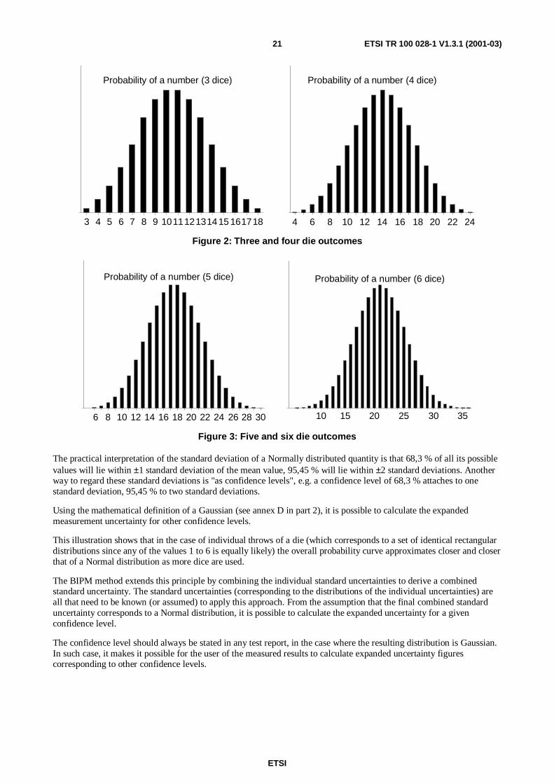
By increasing the number of dice further through 3, 4, 5 and 6 dice it can be seen from figures 2 and 3, that there is acentral value (most probable outcome) respectively for 2, 3, 4, 5 and 6 dice of (7), (10,5), (14), (17,5) and (21) and anassociated spread of the results that increasingly approximates a Normal distribution. It is possible to calculate the meanand standard deviation for these events.
ETSI
ETSI TR 100 028-1 V1.3.1 (2001-03)21
Probability of a number (3 dice) Probability of a number (4 dice)
3 4 5 6 7 8 9 101112131415 161718 4 6 8 10 12 14 16 18 20 22 24
Figure 2: Three and four die outcomes
6 8 10 12 14 16 18 20 22 24 26 28 30
Probability of a number (5 dice)
10 15 20 25 30 35
Probability of a number (6 dice)
Figure 3: Five and six die outcomes
The practical interpretation of the standard deviation of a Normally distributed quantity is that 68,3 % of all its possiblevalues will lie within ±1 standard deviation of the mean value, 95,45 % will lie within ±2 standard deviations. Anotherway to regard these standard deviations is "as confidence levels", e.g. a confidence level of 68,3 % attaches to onestandard deviation, 95,45 % to two standard deviations.
Using the mathematical definition of a Gaussian (see annex D in part 2), it is possible to calculate the expandedmeasurement uncertainty for other confidence levels.
This illustration shows that in the case of individual throws of a die (which corresponds to a set of identical rectangulardistributions since any of the values 1 to 6 is equally likely) the overall probability curve approximates closer and closerthat of a Normal distribution as more dice are used.
The BIPM method extends this principle by combining the individual standard uncertainties to derive a combinedstandard uncertainty. The standard uncertainties (corresponding to the distributions of the individual uncertainties) areall that need to be known (or assumed) to apply this approach. From the assumption that the final combined standarduncertainty corresponds to a Normal distribution, it is possible to calculate the expanded uncertainty for a givenconfidence level.
The confidence level should always be stated in any test report, in the case where the resulting distribution is Gaussian.In such case, it makes it possible for the user of the measured results to calculate expanded uncertainty figurescorresponding to other confidence levels.

ETSI
ETSI TR 100 028-1 V1.3.1 (2001-03)22
For similar reasons, in the case where there is no evidence that the distribution corresponding to the combineduncertainty is Normal, the expansion factor, kxx, should be stated in the test report, instead. Usually, for the reasons
stated above, kxx = 1,96 is used (see also annex D, clause D.5.6.2 of part 2).
An expansion factor, kxx = 2,00 could also be acceptable; it would provide a confidence level of 95,45 % should thecorresponding distribution be Normal.
4.1.4 Main contributors to uncertainty
The main contributors to the overall uncertainty of a measurement comprise:
- systematic uncertainties: those uncertainties inherent in the test equipment used (instruments, attenuators, cables,amplifiers, etc.), and in the method employed. These uncertainties cannot always be eliminated (calculated out)although they may be constant values, however they can often be reduced;
- uncertainties relating to influence quantities i.e. those uncertainties whose magnitudes are dependant on aparticular parameter or function of the EUT. The magnitude of the uncertainty contribution can be calculated, forexample, from the slope of "dB RF level" to "dB SINAD" curve for a receiver or from the slope of a powersupply voltage effect on the variation of a carrier output power or frequency;
- random uncertainties: those uncertainties due to chance events which, on average, are as likely to occur as not tooccur and are generally outside the engineer's control.
NOTE: When making a measurement care must be taken to ensure that the measured value is not affected byunwanted or unknown influences. Extraneous influences (e.g. ambient signals on an Open Area Test Site)should be eliminated or minimized by, for example, the use of screened cables.
4.1.5 Other contributors
Other contributors to the overall uncertainty of a measurement can relate to the standard itself:
- the type of measurement (direct field, substitution or conducted) and the test method have an effect on theuncertainty. These can be the most difficult uncertainty components to evaluate. As an illustration, if the samemeasurand is determined by the same method in different laboratories (as in a round robin) or alternatively bydifferent methods either in the same laboratory or in different laboratories, the results of the testing will often bewidely spread, thereby showing the potential uncertainties of the different measurement types and test methods;
- a direct field measurement involves only a single testing stage in which the required parameter (ERP, sensitivity,etc.) is indirectly determined as the received level on a receiving device, or as the output level of a signalgenerator, etc., and is subsequently converted to ERP, field strength, etc., by a calculation involving knowledgeof antenna gain, measurement distance, etc. This method, whilst being of short time duration, offers no way ofallowing for imperfections (reflections, mutual coupling effects, etc.) in the test site and can results in largeoverall uncertainty values;
- the substitution technique, on the other hand, is a two stage measurement in which the unknown performance ofan EUT (measured in one stage) is directly compared with the "known" performance of some standard (usuallyan antenna) in the other stage. This technique therefore subjects both the EUT and the known standard to(hopefully) the same external influences of reflections, mutual coupling, etc., whose effects on the differentdevices are regarded as identical. As a consequence, these site effects are deemed to cancel out (this has alsobeen addressed in clause D.5.3.2 of annex D, in part 2). Some residual effects do remain however, (due todifferent elevation beamwidths, etc.) but these tend to be small compared to the uncertainties in the direct fieldmethod. All the test methods in the present document are substitution measurements;
- for their part, test methods can contain imprecise and ambiguous instructions which could be open to differentinterpretations;

ETSI
ETSI TR 100 028-1 V1.3.1 (2001-03)23
- an inadequate description of the measurand can itself be a source of uncertainty in a measurement. In practice ameasurand cannot be completely described without an infinite amount of information. Because this definition isincomplete it therefore introduces into the measurement result a component of uncertainty that may or may notbe significant relative to the overall uncertainty required of the measurement. The definition of the measurandmay, for example, be incomplete because:
- it does not specify parameters that may have been assumed, unjustifiably, to have negligible effect(i.e. coupling to the ground plane, reflections from absorbers or that reference conditions remain constant);
- it leaves many other matters in doubt that might conceivably affect the measurement (i.e. supply voltages, thelayout of power, signal and antenna cables);
- it may imply conditions that can never be fully met and whose imperfect realization is difficult to take intoaccount (i.e. an infinite, perfectly conducting ground plane, a free space environment) etc.
Maximum acceptable uncertainties and confidence levels (or expansion factors) are both defined in most ETSIstandards.
4.2 Evaluation of individual uncertainty componentsAs discussed in clause 4.1.4, uncertainty components can be categorized either as "random" or "systematic". Suchcategorization of components of uncertainty can be ambiguous if they are applied too rigorously. For example, a"random" component of uncertainty in one measurement may become a "systematic" component of uncertainty inanother measurement e.g. where the result of a first measurement is used as a component of a second measurement.Categorizing the methods of evaluating the uncertainty components rather than the components themselves avoids thisambiguity.
Instead of "systematic" and "random" uncertainty the types of uncertainty contribution are grouped into two categories:
- Type A: those which are evaluated by statistical methods;
- Type B: those which are evaluated by other means.
The classification into Type A and Type B is not meant to indicate that there is any difference in the nature of thecomponents, it is simply a division based on their means of evaluation. Both types will possess probability distributions(although they may be governed by different rules), and the uncertainty components resulting from either type may bequantified by standard deviations.
4.2.1 Evaluation of Type A uncertainties
When we carry out a measurement more than once and find the results are different, the following questions arise:
- What to do with the results?
- How much variation is acceptable?
- When do we suspect the measuring system is faulty?
- Are the conditions repeatable?
Variations in these repeated measurements are assumed to be due to influence and random quantities that affect themeasurement result and cannot be held completely constant. Therefore none of the results is necessarily correct. Inpractice, repeated measurements of the same measurand can help us evaluate these Type A uncertainties. By treating theresults statistically, we can derive the mean (the best approximation to the "true value") and standard deviation values.The standard deviation can then be incorporated as a standard uncertainty into the calculation of combined standarduncertainty, when the corresponding component is part of some measurement system.
Uncertainties determined from repeated measurements are often thought of as statistically rigorous and thereforeabsolutely correct. This implies, sometimes wrongly, that their evaluation does not require the application of somejudgement. For example:
- When carrying out a series of measurements do the results represent completely independent repetitions or arethey in some way biased?

ETSI
ETSI TR 100 028-1 V1.3.1 (2001-03)24
- Are we trying to assess the randomness of the measurement system, or the randomness in an individual EUT, orthe randomness in all of the EUT produced?
- Are the means and standard deviations constant, or is there perhaps a drift in the value of an unmeasuredinfluence quantity during the period of repeated measurements?
- Are the results stable with ambient conditions?
If all of the measurements are on a single EUT, whereas the requirement is for sampling, then the observations have notbeen independently repeated. An estimate of the standard uncertainty arising from possible differences amongproduction EUT should, in this case, be incorporated into the combined standard uncertainty calculation along with thecalculated standard uncertainty of the repeated observations made on the single equipment (e.g. for characterizing a setof pieces of equipment).
If an instrument is calibrated against an internal reference as part of the measurement procedure, (such as the "cal out"reference on a spectrum analyser), then the calibration should be carried out as part of every repetition, even if it isknown that the drift is small during the period in which observations are made.
If the EUT is rotated during a radiated test on a test site and the azimuth angle read, it should be rotated and read foreach repetition of the measurement, for there may be a variation both in received level and in azimuth reading, even ifeverything else is constant.
If a number of measurements have been carried out on the same EUT/types of EUT, but in two groups spaced apart intime, the arithmetic means of the results of the first and second groups of measurements and their experimentallyderived means and standard deviations may be calculated and compared. This will enable a judgement to be made as towhether any time varying effects are statistically significant.
4.2.2 Evaluation of Type B uncertainties
Some examples of Type B uncertainties are:
- mismatch;
- losses in cables and components;
- non linearities in instruments;
- antenna factors.
Type B uncertainties do not reveal themselves as fluctuations as do Type A uncertainties; they can only be assessed bycareful analysis of test and calibration data.
For incorporation into an overall analysis, the magnitudes and distributions of Type B uncertainties can be estimatedbased on:
- manufacturers' information/specification about instruments and components in the test set-up;
- data in calibration certificates (if the history of the instrument is known);
- experience with the behaviour of the instruments.
4.2.3 Uncertainties relating to influence quantities
Uncertainties relating to influence quantities are, as a result of the way they are treated in the present document,regarded as a subgroup of Type B uncertainties. Some examples of influence quantities are:
- power supply;
- ambient temperature;
- time/duty cycle.
Their effect is evaluated using some relationship between the measured parameter e.g. output power and the influencequantity e.g. supply voltage.

ETSI
ETSI TR 100 028-1 V1.3.1 (2001-03)25
Dependency functions (e.g. the relationship between output power and the fluctuating quantity), as those given in thepresent document, should be used to calculate the properties corresponding to the effect considered.
A theoretical approach to influence quantities and dependency functions can be found in annex D, part 2 (seeclause D.4).
4.3 Methods of evaluation of overall measurement uncertaintyThe uncertainty of the measurement is a combination of many components.
Some of these components may be evaluated from the statistical distributions of the results of a series of measurements(Type A uncertainty) whilst other components are evaluated from assumed probability distributions based onexperience or other information (Type B uncertainty).
The exact error of a result of a measurement is, in general, unknown and unknowable. All that can be done is toestimate the values of all quantities likely to contribute to the combined standard uncertainty, including thoseuncertainties associated with corrections for recognized systematic offset effects. With knowledge of the magnitudes oftheir individual standard uncertainties, it is then possible to calculate the combined standard uncertainty of themeasurement.
At present the assessment of the number of uncertainty components for any particular test is very variable. Whilst somegeneral agreement has been reached on the manner in which individual uncertainties should be combined (the BIPMmethod, see also the discussion of such methods in part 2, annex D, in particular, in clause D.5), no such agreement hasbeen arrived at concerning the identity of those individual components. Consequently, it is left to the particular testhouse/engineer/etc. to decide the contributory uncertainties, and to assess which are independent and which are not.This can lead to considerable test house to test house variation for the same test and is heavily dependent, in general, onthe experience of the test engineer.
A model of the measurement can assist in the evaluation of combined standard uncertainty since it will enable allknown individual components of uncertainty to be rigorously included in the analysis, and correctly combined (seeannex D in part 2, and, in particular, the table in clause D.3.12).
4.4 SummaryThe measured result can be affected by many variables, some of which are shown in figure 4.
Corrections
CouplingEquipment
undertest
Contributions fromthe test method
Influence quantitiesTemperature, supply voltage etc.
Randomuncertainties
Inadequate definitionof the measurand
Statisticalfluctuations
Measuringsystem
Measuredresult
Exisitingknowledge
Systematicuncertainties
Figure 4: The measurement model
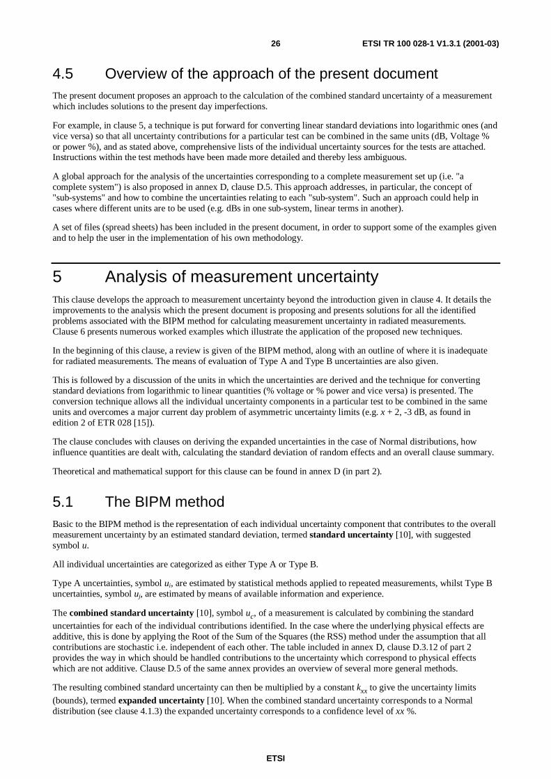
ETSI
ETSI TR 100 028-1 V1.3.1 (2001-03)26
4.5 Overview of the approach of the present documentThe present document proposes an approach to the calculation of the combined standard uncertainty of a measurementwhich includes solutions to the present day imperfections.
For example, in clause 5, a technique is put forward for converting linear standard deviations into logarithmic ones (andvice versa) so that all uncertainty contributions for a particular test can be combined in the same units (dB, Voltage %or power %), and as stated above, comprehensive lists of the individual uncertainty sources for the tests are attached.Instructions within the test methods have been made more detailed and thereby less ambiguous.
A global approach for the analysis of the uncertainties corresponding to a complete measurement set up (i.e. "acomplete system") is also proposed in annex D, clause D.5. This approach addresses, in particular, the concept of"sub-systems" and how to combine the uncertainties relating to each "sub-system". Such an approach could help incases where different units are to be used (e.g. dBs in one sub-system, linear terms in another).
A set of files (spread sheets) has been included in the present document, in order to support some of the examples givenand to help the user in the implementation of his own methodology.
5 Analysis of measurement uncertaintyThis clause develops the approach to measurement uncertainty beyond the introduction given in clause 4. It details theimprovements to the analysis which the present document is proposing and presents solutions for all the identifiedproblems associated with the BIPM method for calculating measurement uncertainty in radiated measurements.Clause 6 presents numerous worked examples which illustrate the application of the proposed new techniques.
In the beginning of this clause, a review is given of the BIPM method, along with an outline of where it is inadequatefor radiated measurements. The means of evaluation of Type A and Type B uncertainties are also given.
This is followed by a discussion of the units in which the uncertainties are derived and the technique for convertingstandard deviations from logarithmic to linear quantities (% voltage or % power and vice versa) is presented. Theconversion technique allows all the individual uncertainty components in a particular test to be combined in the sameunits and overcomes a major current day problem of asymmetric uncertainty limits (e.g. x + 2, -3 dB, as found inedition 2 of ETR 028 [15]).
The clause concludes with clauses on deriving the expanded uncertainties in the case of Normal distributions, howinfluence quantities are dealt with, calculating the standard deviation of random effects and an overall clause summary.
Theoretical and mathematical support for this clause can be found in annex D (in part 2).
5.1 The BIPM methodBasic to the BIPM method is the representation of each individual uncertainty component that contributes to the overallmeasurement uncertainty by an estimated standard deviation, termed standard uncertainty [10], with suggestedsymbol u.
All individual uncertainties are categorized as either Type A or Type B.
Type A uncertainties, symbol ui, are estimated by statistical methods applied to repeated measurements, whilst Type Buncertainties, symbol uj, are estimated by means of available information and experience.
The combined standard uncertainty [10], symbol uc, of a measurement is calculated by combining the standarduncertainties for each of the individual contributions identified. In the case where the underlying physical effects areadditive, this is done by applying the Root of the Sum of the Squares (the RSS) method under the assumption that allcontributions are stochastic i.e. independent of each other. The table included in annex D, clause D.3.12 of part 2provides the way in which should be handled contributions to the uncertainty which correspond to physical effectswhich are not additive. Clause D.5 of the same annex provides an overview of several more general methods.
The resulting combined standard uncertainty can then be multiplied by a constant kxx to give the uncertainty limits
(bounds), termed expanded uncertainty [10]. When the combined standard uncertainty corresponds to a Normaldistribution (see clause 4.1.3) the expanded uncertainty corresponds to a confidence level of xx %.

ETSI
ETSI TR 100 028-1 V1.3.1 (2001-03)27
This is the broad outline of the analysis technique employed in the present document, but there are numerous practicalproblems when applying the basic BIPM rules to measurements, such as:
- how uncertainty contributions in different units (dB, % voltage, % power) can be combined;
- whether individual uncertainties are functions of the true value (e.g. Bit error ratios);
- how to deal with asymmetrically distributed individual uncertainties;
- how to define confidence limits for those standard uncertainties which are not Normal by nature (see alsoclause D.5.6.2 in part 2).
These problem areas are discussed below and have resulted in modifications and extensions to the BIPM method. Formost cases, examples are given in clause 6.
In order to help understanding some of these questions and to bring some more theoretical support, annexes D and E(found in part 2) have been added to the third edition of the present document. Clause D.3 supports variouscombinations (e.g. additive, multiplicative, etc.), conversions (e.g. to and from dBs) and functions (see clauses D.3.9and D.3.11). A complete approach, encompassing the "BIPM method" is included in annex D, clause D.5 (part 2).
5.1.1 Type A uncertainties and their evaluation
Type A uncertainties are evaluated by statistical methods, estimating their standard deviations (corresponding to"standard uncertainties"). These normally play a minor part in the combined standard uncertainty.
Annex D (in part 2) shows that, in most cases, it is only the standard uncertainty that needs to be known in order to findthe combined uncertainty. In the BIPM approach, the shape of the individual distributions is relatively unimportant.However, annex D shows how to combine the various individual distributions, when needed, and that the result of acombination does not necessarily correspond to a Normal distribution. In such a case, the actual shape of the resultingdistribution may be fully relevant (see, in particular, clauses D.5.6.2.3 and D.5.6.2.4).
5.1.2 Type B uncertainties and their evaluation
Type B uncertainties are estimated by various methods.
Figure 5 illustrates a selection of uncertainty distributions which can often be identified in RF measurements.
'U' Distribution
+a-a 0
Rectangular Distribution
+a-a 0
Normal (Gaussian) Distribution
Figure 5: Types of uncertainty distribution
Mismatch uncertainties have the "U" distribution, see annex G. The value of the uncertainty contribution is more likelyto be near the limits than to be small or zero. If the limits are ±a, the standard uncertainty is:
2
a (see annex D).
Systematic uncertainties (e.g. those associated with the loss in a cable) are, unless the actual distribution is known,assumed to have a rectangular distribution. The result of this assumption is that the uncertainty can take any valuebetween the limits with equal probability. If the limits are ±a, the standard uncertainty is:
3
a (see annex D).

ETSI
ETSI TR 100 028-1 V1.3.1 (2001-03)28
If the distribution used to model the uncertainty is a Normal distribution, it is characterized by its standard deviation(standard uncertainty) (see annex D).
In the present document the standard uncertainties are symbolized by uj xx or uj description.
In all cases where the distribution of the uncertainty is unknown, the rectangular distribution should be taken as thedefault model.
It will be noted that all the distributions illustrated in figure 5 are symmetrical about zero (clause D.1, in annex D,addresses also distributions showing an offset and/or which are not symmetrical). An unexpected complication incombining standard uncertainty contributions may result from the use of different units, since a symmetrical standarduncertainty in % voltage is asymmetrical in dB (and vice versa). Similarly for % power. This "major" complication (forany particular test, the contributions may be in a variety of units) is the subject of clause 5.2. See also clause D.3 and inparticular clause D.3.10.7 in annex D, part 2.
5.2 Combining individual standard uncertainties in differentunits
The BIPM method for calculating the combined standard uncertainty of any test involves combining the individualstandard uncertainties by the RSS method. If there are n individual standard uncertainty contributions to be combined,the combined standard uncertainty is:
22)1(
23
22
21
22)1(
23
22
21 .... inniiiijnnjjjjc uu....uuuuu....uuuu ++++++++++++= −− (5.1)
However, this is only correct, if all the individual contributions, represented by their standard uncertainties:
(1) combine by addition; and
(2) are expressed in the same units.
It does not matter whether the contributions are expressed in percent or logarithmic terms or any other terms as long asthese two conditions are fulfilled… noting that the result of the corresponding combination will be expressed in thesame way (see also conversions in clause D.3 and the discussion on the concept of sub-systems in clause D.5 of part 2).
To use formula 5.1 for standard uncertainties of individual contributions which combine by addition, linear terms onlyi.e. voltage, percentage, etc., should be used. This is essential for the RSS combination to be valid. This is the case inmany measuring instruments.
To use formula 5.1 for standard uncertainties of individual contributions which combine by multiplication, logarithmicterms only i.e. dB should be used as they can then be combined by addition. This is essential for the RSS combinationto be valid where uncertainty multiplication occurs. This is the case where gains and/or losses (i.e. attenuators,amplifiers, antennas, etc.) are involved as well as under mismatch conditions where modules (i.e. attenuators, cables,RF measuring instruments, etc.) are interconnected in RF measurements.
If all parameters and their associated standard uncertainties in a measurement are in the same unit and combine byaddition, the RSS method can be applied directly. The table in clause D.3.12 (annex D, part 2) shows how to handleother cases. Clause D.5 (in part 2) discusses general methods usable in most cases.
For small (< 30 % or 2,5 dB) standard uncertainties however, both additive and multiplicative contributions canbe incorporated into the same calculation (with negligible error) provided they are converted to the same unitsprior to calculating the combined standard uncertainty. The conversion factors are given in table 1. This issupported by the theoretical analysis provided in annex D, clause D.3 and annex E (part 2).
Annex E gives the justification for this statement by firstly mathematically converting the distribution of an individualuncertainty from logarithmic to linear (and vice versa) and secondly comparing the standard deviation of the twodistributions before and after the conversion. One of the outcomes of annex E is that the conversion between linear andlogarithmic standard uncertainties can, under some conditions, be approximated by the first order mathematicalfunctions given in table 1.
ETSI
ETSI TR 100 028-1 V1.3.1 (2001-03)29
As can be seen from annex E there are, however, some problems involved in converting distributions.
- It is not a linear procedure; the conversion factor is not only dependent on the magnitude of the standarduncertainty, but it is also dependent on the shape of the distribution.
- The mean value of the converted uncertainty distribution is not necessarily zero, even if that was the case beforethe conversion. However if the standard uncertainties to be converted are less than 2,5 dB, 30 % (voltage), or50 % (power) the errors arising may be considered as negligible.
Table 1 shows the multiplicative factors to be used when converting standard uncertainties with a first orderapproximation. As an example, if the standard uncertainty is 1,5 dB then this, converted to voltage %, gives acorresponding standard uncertainty of 1,5 × 11,5 % = 17,3 %.
Table 1: Standard uncertainty conversion factors
Converting from standarduncertainties in …:
Conversion factormultiply by:
To standarduncertainties in …:
dB 11,5 voltage %dB 23,0 power %
power % 0,0435 dBpower % 0,5 voltage %voltage % 2,0 power %voltage % 0,0870 dB
It should be noted after any conversions that may be necessary before using equation 5.1, that the combined standarduncertainty, uc, that results from the application of equation 5.1, does not, by itself give the expanded uncertainty limitsfor a measurement.
When uc corresponds to a Normal distribution, these can be calculated (see clause 5.3) from uc (assumed in this case to
be in units of dB) as the 95 % confidence limits in dB of ±1,96 × uc (which is very asymmetric in linear terms).
Similarly, in voltage as ±1,96 × uc × 11,5 % (which is very asymmetric in dB terms).The major factor determining
whether the combined standard uncertainty, uc, will have the symmetrical dB interval or the symmetrical % interval (or
somewhere in-between) is whether the individual uncertainties combine by multiplication or by addition. In radiatedmeasurements as well as most conducted measurements where the RF level is of importance, the overwhelmingmajority of the uncertainties combine by multiplication. It is, therefore, safe to assume that, in general, the resultinguncertainty limits are symmetrical in logarithmic terms (dB). This assumption has been confirmed by computersimulations on a large number of measurement models. This is also clear from the relations found in annex D.
As shown in annex F, the shapes of the individual distributions only matter if they are very large (compared to the rest).
5.3 Calculation of the expanded uncertainty values andStudent's t-distribution
This clause discusses two different problems, both relating to the handling of uncertainties, which have to be veryclearly identified and handled separately. Unfortunately, in the previous editions of the present document, this clausehad not been subdivided into two clauses.
The two clauses address:
- the situation where the statistical properties of a number of samples are to be evaluated; in this case, theStudent's t-distribution is a powerful tool allowing to evaluate the performance of those properties; it can behelpful in supporting the evaluation of properties of "type A uncertainties";
- the situation where only one measurement is performed, in conditions where the various sources of uncertaintyhave been evaluated; as a result, the combined standard uncertainty of that measurement may be evaluated (seeannex D, clause D.5, in part 2), and the knowledge of the shape of the distribution corresponding to thatcombined uncertainty allows for changes in the confidence level.

ETSI
ETSI TR 100 028-1 V1.3.1 (2001-03)30
5.3.1 Student's t-distribution
The Student's t-distribution gives coverage factors (i.e. multipliers) for measurements, whereby the confidence level ofa series of measurement can be calculated from a limited number of samples, assuming those samples have been takenfrom a Normal distribution. The fewer the number of samples, the bigger the coverage factor for a given confidencelevel.
For example:
- if a type A standard deviation is calculated on only 3 samples and the required confidence level is 95 % theappropriate Student's t-factor is 3,18;
- if the standard deviation had been based on 20 samples, the factor would have been 2,09;
- for an infinite number of samples the multiplier would have been 1,96.
When using such an approach, any measurement should be repeated a large number of times.
In radio measurements, however, by using the approach recommended in the present document, only one measurementis usually performed. As a result, the Student's t-distribution is of no help.
The Student's t-distribution can, however, be very useful for the statistical evaluation of the properties of individualuncertainty components (i.e. type A uncertainties which may happen to be part of some test set up).
5.3.2 Expanded uncertainties
When the combined standard uncertainty, uc, has been calculated from equation 5.1 (or by any other method) and it can
be expected that the corresponding distribution is Normal, then, the uncertainty limits relate to a confidence level of68,3 % (due to the properties of the Gaussian curve).
By multiplying uc by "a coverage factor" (or "an expansion factor") other confidence levels may be obtained when the
distribution corresponding to the combined standard uncertainty, uc, is Normal. Why?
When:
- all the individual sources of uncertainty are identified for all the tests;
- the distributions of the uncertainties of the individual sources are all known (or assumed);
- the maximum, worst-case values of all of the individual uncertainties are known.
Then, under these conditions, annex D of part 2 applies and the combined standard uncertainty can be calculated (seeclause D.5).
Assuming that the combined standard uncertainty corresponds to a Normal distribution then the magic factor of 1,96applies: this is due to the shape of the Gaussian curve used to describe the distribution corresponding to the combineduncertainty (see the interpretation in clause D.5.6.2 of annex D, part 2).
As already indicated above (see clause 4.1.3), for a Gaussian shaped curve:
- a surface of 68 % (2 x 34 %) corresponds to one standard deviation (i.e. a combined standard deviation);
- a surface of 95 % (2 x 47,5 %) corresponds to two standard deviations (more precisely 1,96 standard deviations).
And the surface refereed above can be interpreted as the probability of the true value being within the stated uncertainty(which, in turn, corresponds to the confidence level).
It has to be made clear that, when the combination of the various components of the uncertainty correspond to adistribution which is not Normal, then other factors apply in order to convert from one confidence level to another.These factors depend on the shape (and mathematical properties) of the corresponding distribution.
It has to be made clear also that, as indicated in particular in annex D, when the number of components used to calculatethe uncertainty can be considered as an infinity, and under some other conditions, then the distribution can beconsidered as Normal. Under such conditions, the factor 1,96 appears to be valid. This is why it has been used all overthe examples given in the present document.

ETSI
ETSI TR 100 028-1 V1.3.1 (2001-03)31
The usage of a value of 2 for this expansion factor has also been suggested (this would provide a confidence level of95,45 % in the case of Normal distributions).
The tools given in annex D could allow for the calculation of the actual distribution corresponding to the combination ofvarious components for the uncertainty. Under such conditions, the appropriate expansion factors could also becalculated, in the case where the distribution found would not have happened to be Normal.
5.4 Combining standard uncertainties of different parameters,where their influence on each other is dependant on theEUT (influence quantities)
In many measurements, variations in the influence quantities, intermediate test results or test signals can affect theuncertainty of the measurand in ways that may be functions of the characteristics of the EUT and other instrumentation.
It is not always possible to fully characterize test conditions, signals and measurands. Uncertainties are related to eachof them. These uncertainties may be well known, but their influence on the combined standard uncertainty depends onthe EUT. Uncertainties related to general test conditions are:
- ambient temperature;
- the effect of cooling and heating;
- power supply voltage;
- power supply impedance;
- impedance of test equipment connectors (VSWR).
Uncertainties related to applied test signals and measured values are:
- level;
- frequency;
- modulation;
- distortion;
- noise.
The effect of such uncertainties on the test results can vary from one EUT to another. Examples of the characteristicsthat can affect the calculation of the uncertainties are:
- receiver noise dependency of RF input signal levels;
- impedance of input and output connectors (VSWR);
- receiver noise distribution;
- performance dependency of changes of test conditions and test signals;
- modulator limiting function e.g. maximum deviation limiting;
- system random noise.
If the appropriate value for each characteristic has not been determined for a particular case, then the values listed inpart 2, annex F, table F.1 should be used. These values are based on measurements made with several pieces ofequipment and are stated as mean values associated with a standard uncertainty reflecting the spread from one EUT toanother.

ETSI
ETSI TR 100 028-1 V1.3.1 (2001-03)32
When the EUT dependent uncertainties add to the combined standard uncertainty, the RSS method of combining thestandard uncertainties is used, but in many calculations the EUT dependency is a function that converts uncertaintyfrom one part of the measurement configuration to another. In most cases the function can be assumed to be linear;therefore the conversion is carried out by multiplication. A theoretical analysis ir provided in clause D.4 of annex D, inpart 2.
The standard uncertainty to be converted is uj 1. The mean value of the influence quantity is A and its standard
uncertainty is uj a. The resulting standard uncertainty uj converted of the conversion is:
)+uA(u=u ajjconvertedj222
1 (5.2)
The standard uncertainty of this contribution is then looked upon as any other individual component and is combinedaccordingly (see annex D). A fully worked example of an influence quantity is given in clause 6.4.6. The conditionsunder which the expression 5.2 is valid can also be found in clause D.4 of annex D, in part 2.
If the function is not linear another solution must be found:
- the theoretical relation between the influence quantity and its effect has to be determined;
- the expressions providing the conversion can then be found based on the table contained in clause D.3.12 ofannex D (part 2).
When the theoretical relation between the influence quantity and its effect is not known, the usage of a simplemathematical model can be tried. In this case, an attempt can be made in order to determine the numerical values of theparameters of the model by some statistical method (see also clause D.5.4 in part 2).
In all cases, it is recommended to determine first the mathematical relation between the parameters, and only after tryand find the appropriate numerical values. As a consequence, tables similar to table F.1 in annex F (part 2) should alsoinclude the mathematical relation between the parameters for each entry (for further details, see clause D.4.2.1.2 inpart 2).
5.5 Estimate of standard uncertainty of randomnessThe major difficulty behind this clause is to evaluate what exactly it is supposed to cover: the BIPM method and thecorresponding analysis is supposed to cover all components of the uncertainty, so it is fundamental to understand whatis left over for the "uncertainty of randomness", and avoid taking into account the same effects in a complex set uptwice, under different names…
The standard uncertainty of randomness can be evaluated by repeating a measurement (e.g. of a particular componentof the measurement uncertainty).
The first step is to calculate the arithmetic mean or average of the results obtained.
The spread in the measured results reflects the merit of the measurement process and depends on the apparatus used, themethod, the sample and sometimes the person making the measurement. A more useful statistic, however, is thestandard uncertainty σi of the sample. This is the root mean square of the sum of the differences of the measured valueminus the arithmetic mean of the sample.
If there are n results for xm where m = 1, 2, ..., n and the sample mean is x, then the standard deviation σi is:
∑=
−
n
m
_
mi xxn
=
1
21σ (5.3)
This should not be confused with the standard deviation of the A uncertainty being investigated. It only covers nsamples.
If further measurements are made, then for each sample of results considered, different values for the arithmetic meanand standard deviation will be obtained. For large values of n these mean values approach a central limit value of adistribution of all possible values. This distribution can usually be assumed, for practical purposes, to be a Normaldistribution.

ETSI
ETSI TR 100 028-1 V1.3.1 (2001-03)33
From the results of a relatively small number of measurements an estimate can be made of the standard deviation of thewhole population of possible values, of which the measured values are a sample.
Estimate of the standard deviation σi/:
2
1
/
1
1
−= ∑
_
m
n
m=
i xx)n-
(σ (5.4)
A practical form of this formula is:
1
2
/
n -n
XY -
i =σ (5.5)
where X is the sum of the measured values and Y is the sum of the squares of the measured values.
It will be noted that the only difference between σi/ and σi is in the factor 1/ (n-1) in place of 1/n, so that the difference
becomes smaller as the number of measurements is increased. A similar way of calculating the standard deviation of adiscrete distribution can be derived from this formula.
In this case X is the sum of the individual values from the distribution times their probability, and Y is the sum of thesquare of the individual values times their probability.
If the distribution has m values xi, each having the probability p (xi):
)p(xxX i
m
i
i∑=
=1
(5.6)
and
)p(xxY i
m
i
i∑=
=1
2 (5.7)
The standard uncertainty is then:
2XYi −=σ (5.8)
When a measured results is obtained as the arithmetic mean of a series of n (independent) measurements the standarduncertainty is reduced by a factor √n thus:
n=i
/1σ
σ (5.9)
This is an efficient method of reducing measurement uncertainty when making noisy or fluctuating measurements, andit applies both for random uncertainties in the measurement configuration and the EUT. Having established the standarddeviation, this is directly equated to the standard uncertainty:
ui = σi
As the uncertainty due to random uncertainty is highly dependent on the measurement configuration and thetest method used it is not possible to estimate a general value.
Each laboratory must by means of repetitive measurements estimate their own standard uncertainties characterizing therandomness involved in each measurement. Once having done this, the estimations may be used in future measurementsand calculations.
NOTE: See also the note found in clause 6.4.7 concerning the usage of this component.

ETSI
ETSI TR 100 028-1 V1.3.1 (2001-03)34
5.6 Summary of the recommended approachThe basic BIPM method, with specific modifications, remains the adopted approach used for the calculation ofcombined standard and expanded uncertainty in the examples given in this report for radiated measurements. That is tosay that once all the individual standard uncertainties in a particular measurement have been identified and givenvalues, they are combined by the RSS method provided they combine by addition and are in the same units(otherwise, methods such as those detailed in annex D, e.g. in clause D.5, have to be used).
In order to ensure that this proviso is satisfied as often as possible, the present document supplies the factors necessaryto convert standard uncertainties in linear units to standard uncertainties in logarithmic units (and vice versa). Thepresent document also shows that small additive standard uncertainties (% V, % power) can be combined withmultiplicative standard uncertainties (dB) in the RSS manner with, hopefully, negligible error.
Having derived the combined standard uncertainty, an expanded uncertainty for 95 % confidence levels can then bederived, when the corresponding distribution is Normal, by multiplying the result by the expansion factor of 1,96. Themultiplication by this factor (or simply by a factor equal to 2) is to be done in all cases, in order to obtain the expandeduncertainty. However, if the corresponding distribution is not Normal, then the resulting confidence level is notnecessarily 95 % (see clause D.5.6.2 in annex D, part 2). In all cases, however, the actual confidence level can becalculated, once the distribution corresponding to the combination of all uncertainty components has been calculated.Clause D.3, in part 2, provides the equations allowing for the calculation of this combined distribution.
The practical implementation of this modified BIPM approach, adopted throughout the present document, is for eachtest method (including the verification procedures) to have appended to it a complete list of the individual uncertaintysources that contribute to each stage of the test. Magnitudes of the standard uncertainties can then be assigned to theseindividual contributions by consulting annex A (converting from linear units to dB, if necessary). All uncertainties arein dB units since the great majority of the individual contributions in radiated measurements are multiplicative i.e. theyadd in dB terms.
In those cases in which annex A instructs that the values of the uncertainty contributions be taken from a manufacturer'sdata sheet, that data should be taken over as broad a frequency band as possible. This type of approach avoids thenecessity of calculating the combined standard uncertainty every time the same test is performed for differentEUT.
6 Examples of uncertainty calculations specific to radioequipment
6.1 MismatchIn the following the Greek letter Γ means the complex reflection coefficient. ρx is the magnitude of the reflectioncoefficient: ρx = Γx.
Where two parts or elements in a measurement configuration are connected, if the matching is not ideal, there will be anuncertainty in the level of the RF signal passing through the connection. The magnitude of the uncertainty depends onthe VSWR at the junction of the two connectors.
The uncertainty limits of the mismatch at the junction are calculated by means of the following formula:
Mismatch limits = |Γgenerator| × |Γload| × |S21| × |S12| × 100 % Voltage (6.1)
where:
|Γgenerator| is the modulus of the complex reflection coefficient of the signal generator;
|Γload| is the modulus of the complex reflection coefficient of the load (receiving device);
| S21| is the forward gain in the network between the two reflection coefficients of interest;
| S12| is the backward gain in the network between the two reflection coefficients of interest.
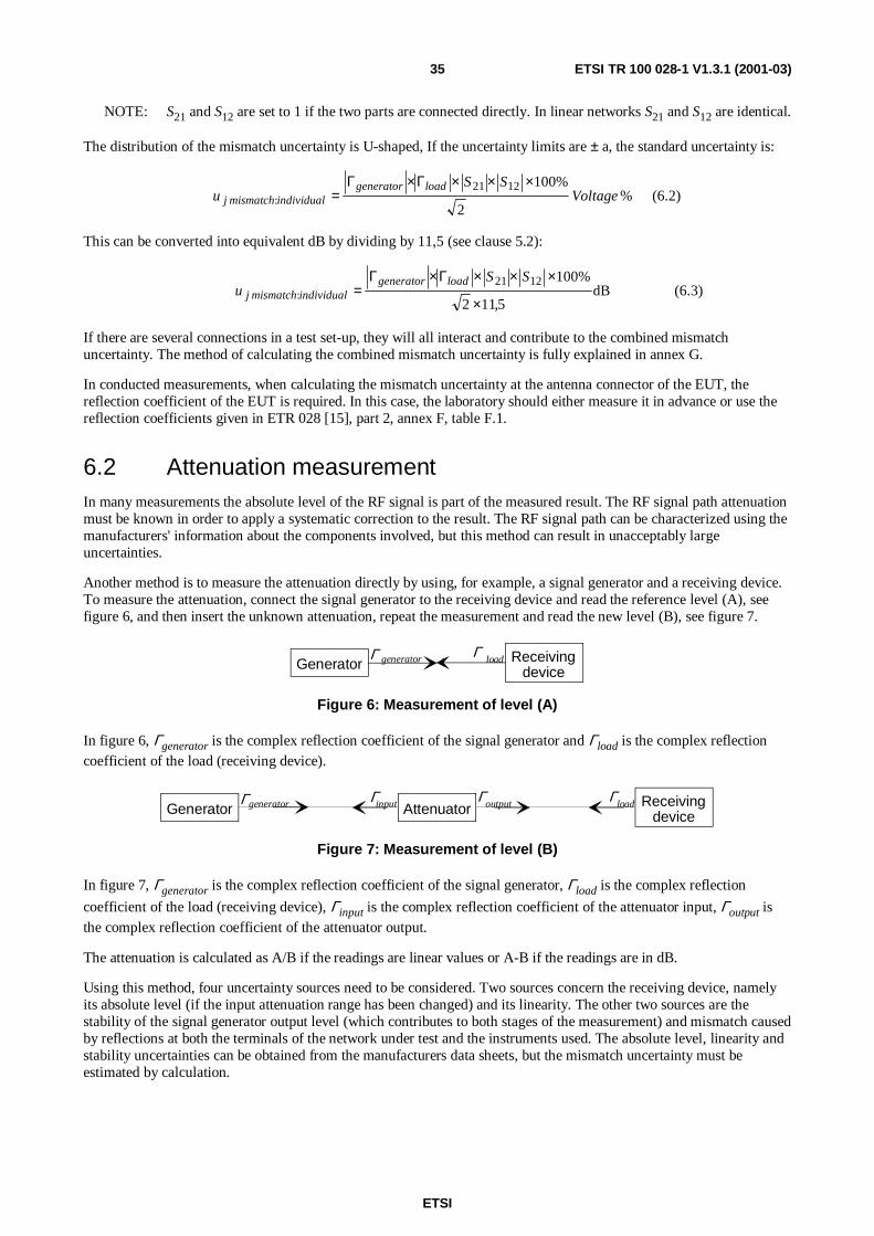
ETSI
ETSI TR 100 028-1 V1.3.1 (2001-03)35
NOTE: S21 and S12 are set to 1 if the two parts are connected directly. In linear networks S21 and S12 are identical.
The distribution of the mismatch uncertainty is U-shaped, If the uncertainty limits are ± a, the standard uncertainty is:
%2
%1001221: Voltage
SSu
loadgeneratorindividualj mismatch
×××Γ×Γ= (6.2)
This can be converted into equivalent dB by dividing by 11,5 (see clause 5.2):
dB5,112
%1001221:
×
×××Γ×Γ=
SSu
loadgeneratorindividualj mismatch (6.3)
If there are several connections in a test set-up, they will all interact and contribute to the combined mismatchuncertainty. The method of calculating the combined mismatch uncertainty is fully explained in annex G.
In conducted measurements, when calculating the mismatch uncertainty at the antenna connector of the EUT, thereflection coefficient of the EUT is required. In this case, the laboratory should either measure it in advance or use thereflection coefficients given in ETR 028 [15], part 2, annex F, table F.1.
6.2 Attenuation measurementIn many measurements the absolute level of the RF signal is part of the measured result. The RF signal path attenuationmust be known in order to apply a systematic correction to the result. The RF signal path can be characterized using themanufacturers' information about the components involved, but this method can result in unacceptably largeuncertainties.
Another method is to measure the attenuation directly by using, for example, a signal generator and a receiving device.To measure the attenuation, connect the signal generator to the receiving device and read the reference level (A), seefigure 6, and then insert the unknown attenuation, repeat the measurement and read the new level (B), see figure 7.
Receivingdevice
ΓloadGenerator
Γ generator
Figure 6: Measurement of level (A)
In figure 6, Γgenerator is the complex reflection coefficient of the signal generator and Γload is the complex reflectioncoefficient of the load (receiving device).
Generator Attenuator Receivingdevice
Γload
ΓoutputΓgenerator Γinput
Figure 7: Measurement of level (B)
In figure 7, Γgenerator is the complex reflection coefficient of the signal generator, Γload is the complex reflection
coefficient of the load (receiving device), Γinput is the complex reflection coefficient of the attenuator input, Γoutput isthe complex reflection coefficient of the attenuator output.
The attenuation is calculated as A/B if the readings are linear values or A-B if the readings are in dB.
Using this method, four uncertainty sources need to be considered. Two sources concern the receiving device, namelyits absolute level (if the input attenuation range has been changed) and its linearity. The other two sources are thestability of the signal generator output level (which contributes to both stages of the measurement) and mismatch causedby reflections at both the terminals of the network under test and the instruments used. The absolute level, linearity andstability uncertainties can be obtained from the manufacturers data sheets, but the mismatch uncertainty must beestimated by calculation.
ETSI
ETSI TR 100 028-1 V1.3.1 (2001-03)36
For this example, we assume that an attenuator of nominally 20 dB is measured at a frequency of 500 MHz by means ofa signal generator and a receiving device. The magnitude of the reflection coefficient of the generator |Γgenerator| is 0,2,
the magnitude of the reflection coefficient of the receiving device |Γload| is 0,3 and the magnitude of the reflection
coefficients of the attenuator |Γinput| and |Γoutput| are 0,05.
Since the mismatch uncertainty of the attenuation measurement is different in figure 7 to that in figure 6, it therefore hasto be calculated (for figure 6 and figure 7) and both values included in the combined mismatch uncertainty as shownbelow.
Mismatch uncertainty:
Reference measurement: The signal generator is adjusted to 0 dBm and the reference level A is measured on thereceiving device. Using equation 6.1 with S21 = S12 = 1, and taking the standard uncertainty,
uj mismatch: reference measurement:
dB0,37511
244%24,4%
2
1003020: =
,
,,,u tmeasuremenreferencej mismatch ≈=××=
Attenuator measurement: The attenuator is inserted and a level (B) = -20,2 dB is measured after an input attenuationrange change on the receiving device.
NOTE: The measured attenuation is 20,2 dB, for which S21 = S12 = 0,098.
The following three components comprise the uncertainty in this part of the measurement:
- the standard uncertainty of the mismatch between the signal generator and the attenuator:
%0,71%2
10005020: =××= ,,
u attenuatortogeneratorj mismatch
- the standard uncertainty of the mismatch between the attenuator and the receiving device:
%,061%2
10005030: =××= ,,
u devicereceivingtoattenuatorj mismatch
- the standard uncertainty of the mismatch between the signal generator and the receiving device:
%,0410%2
100098,02030 2
: =×××= ,,u devicereceivingtogeneratorj mismatch
The combined standard uncertainty of the mismatch of the attenuation measurement uc mismatch: att. measurement, is
calculated by RSS (clause 5.2) of the individual contributions.
dB0,11511
281%,2810410061710 222
.: =≈=++=,
,,,,u tmeasuremenattc mismatch
A comparison of uj mismatch: reference measurement (0,37 dB) and uc mismatch: att. measurement (0,11 dB) shows clearly theimpact of inserting an attenuator between two mismatches.
Other components of uncertainty:
Reference measurement: The stability of the signal generator provides the only other uncertainty in this part. Thereceiving device contributes no uncertainty here since only a reference level is being set for comparison in theattenuation measurement stage.

ETSI
ETSI TR 100 028-1 V1.3.1 (2001-03)37
The output level stability of the signal generator is taken from the manufacturer's data sheet as 0,10 dB which isassumed (since no information is given) to be rectangularly distributed (see clause 5.1). Therefore the standarduncertainty, uj signal generator stability, is:
dB0,063
100=
,u stabilitygeneratorj signal =
Therefore, the combined standard uncertainty, uc reference measurement, for the reference measurement is:
dB0,37060370 2222: =+=+= ,,uuu stabilitygeneratorsignaljtmeasuremenreferencemismatchjtmeasuremenreferencec
Attenuation measurement: Here the output stability of the signal generator as well as absolute level uncertainty of thereceiving device (the input attenuation range has changed) contribute to the uncertainty. However as a range change hasoccurred there is no linearity contribution as this is included in the absolute level uncertainty of the receiver.
The signal generator stability, uj signal generator stability, has the same value as for the reference measurement, whilst the
uncertainty for the receiving device is given in the manufacturer's data sheet as 1,0 dB absolute level accuracy. Arectangular distribution is assumed for the absolute level accuracy so the standard uncertainty, uj signal generator level, ofits uncertainty contribution is:
dB0,583
001 == ,u levelgeneratorj signal
The uncertainty contribution of the linearity of the receiving device uj linearity is zero.
Therefore the combined standard uncertainty, uc att. measurement, for the attenuation measurement is:
2222.:. yj linearitlevelgeneratorj signalstabilitygeneratorj signaltmeasuremenattc mismatchtmeasuremenc att uuuuu +++=
dB0,59000580060080 2222 =+++= ,,,,
So, for the complete measurement, the combined standard uncertainty, uc measurement, is given by:
dB0,70590370 222.
2 =+=+= ,,uuu tmeasuremenc atttmeasuremenec referenctmeasuremenc
The expanded uncertainty is ±1,96 × 0,70 = ±1,37 dB at a 95 % confidence level.
This is an exaggerated example. Smaller uncertainty is possible if a better receiving device is used.
6.3 Calculation involving a dependency functionThe specific dependency function is the relationship between the RF signal level at the EUT antenna connector (dB) tothe uncertainty of the measurement of SINAD at the EUT's audio output i.e. how does SINAD measurement uncertaintyrelate to RF level uncertainty at the EUT antenna connector.
The following example is based on a typical ETR 028 [15] type (conducted) RF measurement for clarity. The sensitivityof a receiving EUT is measured. The outline of the measurement is as follows. The RF level at the input of the receiveris continuously reduced until a SINAD measurement of 20 dB is obtained, see figure 8.
The result of the measurement is the RF signal level causing 20 dB SINAD at the audio output of the receiver.

ETSI
ETSI TR 100 028-1 V1.3.1 (2001-03)38
SINADmeterEUT dependancy function
mean value = 1standard deviation = 0,3
EUT
± 1,0 dB ± 1,0dB
Signalgenerator
| = 0,07|S11
| | = 0,07S22
± 0,5dBcable
|ρgenerator|= 0,30
|ρ |= 0,4EUT
Figure 8: Typical measurement configuration
The combined standard uncertainty is calculated as follows.
For the mismatch uncertainty (annex G):
Generator: Output reflection coefficient: |ρgenerator| = 0,30
Cable: Input and output reflection coefficients: |S11| and |S22| = 0,07
Attenuation: 1 dB = |S21| = |S12| = 0,891
EUT: Input reflection coefficient: |ρEUT| = 0,4
All these contributions are U distributed. There are three contributions:
- the standard uncertainty of the mismatch between the signal generator and the cable:
dB0,135112
%100070300: =
×××=,
,,u cabletogeneratorsignalj mismatch
- the standard uncertainty of the mismatch between the cable and the EUT:
dB0,175112
%10007040: =
×××=
,
,,u EUTtocablej mismatch
- the standard uncertainty of the mismatch between the signal generator and the EUT:
dB0,595112
%10089104030 2
: =×
×××=,
,,,u EUTtogeneratorsignalj mismatch
- the combined standard uncertainty of the mismatch:
,63dB059,017,013,0 222 =++=c mismatchu
uc mismatch = 0,63 dB
The uncertainty due to the absolute output level of the signal generator is taken as ±1,0 dB (from manufacturers data).As nothing is said about the distribution, a rectangular distribution in logs is assumed (see clause 5.1), and the standarduncertainty is:
uj signal generator level = 0,58 dB
The uncertainty due to the output level stability of the signal generator is taken as ±0,02 dB (from manufacturer's data).As nothing is said about the distribution, a rectangular distribution in logs is assumed (see clause 5.1), and the standarduncertainty is:
uj signal generator stability = 0,01 dB
The uncertainty due to the insertion loss of the cable is taken as ±0,5 dB (from calibration data). As nothing is saidabout the distribution, a rectangular distribution in logs is assumed, and the standard uncertainty is:
uj cable loss = 0,29 dB
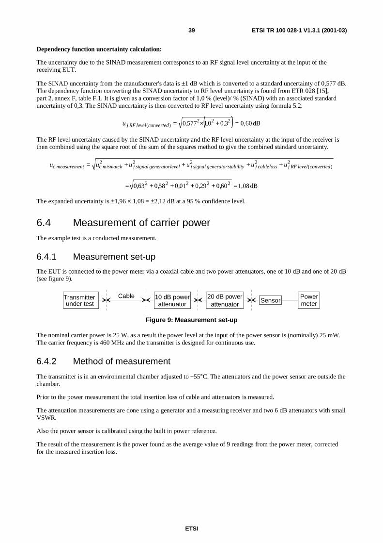
ETSI
ETSI TR 100 028-1 V1.3.1 (2001-03)39
Dependency function uncertainty calculation:
The uncertainty due to the SINAD measurement corresponds to an RF signal level uncertainty at the input of thereceiving EUT.
The SINAD uncertainty from the manufacturer's data is ±1 dB which is converted to a standard uncertainty of 0,577 dB.The dependency function converting the SINAD uncertainty to RF level uncertainty is found from ETR 028 [15],part 2, annex F, table F.1. It is given as a conversion factor of 1,0 % (level)/ % (SINAD) with an associated standarduncertainty of 0,3. The SINAD uncertainty is then converted to RF level uncertainty using formula 5.2:
( ) dB0,60=30015770 222)( ,,,u convertedlevelj RF +×=
The RF level uncertainty caused by the SINAD uncertainty and the RF level uncertainty at the input of the receiver isthen combined using the square root of the sum of the squares method to give the combined standard uncertainty.
2)(
2222convertedlevelj RFlossj cablestabilitygeneratorj signallevelgeneratorj signalc mismatchentc measurem uuuuuu ++++=
dB1,08=600290010580630 22222 ,,,,,= ++++
The expanded uncertainty is ±1,96 × 1,08 = ±2,12 dB at a 95 % confidence level.
6.4 Measurement of carrier powerThe example test is a conducted measurement.
6.4.1 Measurement set-up
The EUT is connected to the power meter via a coaxial cable and two power attenuators, one of 10 dB and one of 20 dB(see figure 9).
Transmitterunder test
PowermeterSensor
20 dB powerattenuator
10 dB powerattenuator
Cable
Figure 9: Measurement set-up
The nominal carrier power is 25 W, as a result the power level at the input of the power sensor is (nominally) 25 mW.The carrier frequency is 460 MHz and the transmitter is designed for continuous use.
6.4.2 Method of measurement
The transmitter is in an environmental chamber adjusted to +55°C. The attenuators and the power sensor are outside thechamber.
Prior to the power measurement the total insertion loss of cable and attenuators is measured.
The attenuation measurements are done using a generator and a measuring receiver and two 6 dB attenuators with smallVSWR.
Also the power sensor is calibrated using the built in power reference.
The result of the measurement is the power found as the average value of 9 readings from the power meter, correctedfor the measured insertion loss.

ETSI
ETSI TR 100 028-1 V1.3.1 (2001-03)40
6.4.3 Power meter and sensor module
The power meter uses a thermocouple power sensor module and contains a power reference.
Power reference level:
Power reference level uncertainty: ±1,2 % power.
As nothing is stated about the distribution it is assumed to be rectangular and the standard uncertainty is convertedfrom % power to dB by division with 23,0 (see clause 5.2).
Standard uncertainty dB0,0300233
21 =×
=,
,u levelej referenc .
Mismatch whilst measuring the reference:
Reference source VSWR: 1,05 (d): ρreference source = 0,024;
Power sensor VSWR: 1,15 (d): ρload = 0,07.
Using formula 6.3 the standard uncertainty of the mismatch is:
dB0,0105112
%1000700240: =
×
××=
,
,,u referencej mismatch
Calibration factors:
Calibration factor uncertainty = ±2,3 % power.
As nothing is stated about the distribution it is assumed to be rectangular. The standard uncertainty is converted from %power to dB by division with 23,0.
standard uncertainty dB0,0580233
32 =×
=,
,u factorionj calibrat
Range to range change:
Range to range uncertainty (one change) = ±0,5 % power.
As nothing is stated about the distribution it is assumed to be rectangular. The standard uncertainty is converted from %power to dB by division with 23,0.
standard uncertainty dB0,0060233
250 =×
=,
,u changerangej
Noise and drift is negligible at this power level and can be ignored.
Combined standard uncertainty of the power meter and sensor:
Using formula 5.1:
222:
2changej rangefactorionj calibratreferencej mismatchlevelej referencsensorandc meter uuuuu +++=
dB0,066006005800100030 2222 =+++= ,,,,u sensorandc meter

ETSI
ETSI TR 100 028-1 V1.3.1 (2001-03)41
6.4.4 Attenuator and cabling network
Standing wave ratios involved in the attenuation measurement (taken from manufacturers data):
- Signal generator: VSWR ≤ 1,5 ρ = 0,200
- Power sensor: VSWR ≤ 1,15 ρ = 0,070
- 6 dB attenuators: VSWR ≤ 1,2 ρ = 0,091
- 10 dB power attenuator: VSWR ≤ 1,3 ρ = 0,130
- 20 dB attenuator: VSWR ≤ 1,25 ρ = 0,111
- Cable: VSWR ≤ 1,2 ρ = 0,091
Nominal attenuations converted to linear values:
- 6 dB = S21 = S12 = 0,500;
- 10 dB = S21 = S12 = 0,316;
- 20 dB = S21 = S12 = 0,100;
- 0,3 dB = S21 = S12 = 0,966 (assumed cable attenuation in the uncertainty calculations).
The attenuation measurement is carried out using a signal generator and a measuring receiver. In order to have a lowVSWR two 6 dB attenuators with low reflection coefficients are inserted.
The measurement of the attenuation in the attenuator and cabling network is carried out by making a referencemeasurement (figure 10). The measurement receiver reading is "A" dBm.
Then the cables and the attenuators are inserted. First the cable and the 10 dB power attenuator is inserted between thetwo 6 dB attenuators, and a new reading "B" dBm is recorded (see figure 11).
Finally the 20 dB attenuator is inserted between the two 6 dB attenuators, and the reading "C" dBm is recorded (seefigure 12).
The total attenuation is then ("A"-"B") dB + ("A"-"C") dB.
6.4.4.1 Reference measurement
Figure 10 details the components involved in this reference measurement.
6 dB (2)attenuator
6 dB (1)attenuator
RF signal
generatorPower meterand sensor
Figure 10: The reference measurement
The individual mismatch uncertainties between the various components in figure 10 are calculated using formula 6.3:
- the standard uncertainty of the mismatch between the signal generator and 6 dB attenuator (1):
dB0,1125112
%100091020.6: =
×××=,
,,u attdBtogeneratorj mismatch
- the standard uncertainty of the mismatch between the 6 dB attenuator (1) and 6 dB attenuator (2):
dB0,0515112
%100091009102.61.6: =
×××=,
,,u attdBtoattdBj mismatch

ETSI
ETSI TR 100 028-1 V1.3.1 (2001-03)42
- the standard uncertainty of the mismatch between the 6 dB attenuator (2) and power sensor:
dB0,0395112
%1000700910.6: =
×××=,
,,u sensorpowertoattdBj mismatch
- the standard uncertainty of the mismatch between the signal generator and 6 dB attenuator (2):
dB0,0285112
%10050091020 2
2.6: =×
×××=,
,,,u attdBtogeneratorj mismatch
- the standard uncertainty of the mismatch between the 6 dB attenuator (1) and power sensor:
dB0,0105112
%100500700910 2
1.6: =×
×××=,
,,,u sensorpowertoattdBj mismatch
- the standard uncertainty of the mismatch between the signal generator and power sensor:
dB0,0055112
%100505007020 22
: =×
××××=,
,,,,u sensorpowertogeneratorj mismatch
It can be seen that the mismatch uncertainty between the RF signal generator and the 6 dB attenuator (1) uj generator to
6 dB att 1, and the mismatch uncertainty between the 6 dB attenuator (2) and the power sensor uj 6 dB att. 2 to power sensor,
add to both the reference measurement and the measurements with the unknown attenuators inserted.
It is the result of the methodology adopted in annex D that these terms cancel and hence do not contribute to thecombined standard uncertainty of the final result. The reference measurement mismatch uncertainty uj mismatch: reference
(formula 5.1):
221.6
22.6
22.61.6: sensorpowertorj generatosensorpowertoattdBjattdBtorj generatoattdBtoattdBjreferencej mismatch uuuuu +++=
dB0,0590050010002800510 2222: =+++= ,,,,u referencej mismatch
NOTE: If the two uncertainties of the generator and the power sensor did not cancel due to the methodology, thecalculated reference measurement uncertainty would have been 0,131 dB.
6.4.4.2 The cable and the 10 dB power attenuator
Figure 11 shows the clause of the reference set-up which concerns this part of the calculation.
6 dB (2)attenuator
RF signalgenerator
6 dB (1)attenuator
Cable 10 dB powerattenuator
Power meterand sensor
Figure 11: The cable and the 10 dB power attenuator
The individual uncertainties are calculated using formula 6.3:
- the standard uncertainty of the mismatch between the signal generator and 6 dB attenuator (1):
dB0,1125112
%100091020.6: =
×××=,
,,u attdBtogeneratorj mismatch
- the standard uncertainty of the mismatch between the 6 dB attenuator (1) and cable:
dB0,0515112
%100091009101.6: =
×××
=,
,,u cabletoattdBj mismatch

ETSI
ETSI TR 100 028-1 V1.3.1 (2001-03)43
- the standard uncertainty of the mismatch between the cable and 10 dB power attenuator:
dB0,0735112
%10013000910.10: =
×××
=,
,,u attdBtocablej mismatch
- the standard uncertainty of the mismatch between the 10 dB attenuator and the 6 dB attenuator (2):
dB0,0735112
%100091013002.6.10: =
×××=,
,,u attdBtoattdBj mismatch
- the standard uncertainty of the mismatch between the 6 dB attenuator (2) and power sensor:
dB0,0395112
%1000700910.6: =
×××=,
,,u sensorpowertoattdBj mismatch
- the standard uncertainty of the mismatch between the signal generator and cable:
dB0,0285112
%1005009102000 2
: =×
×××=,
,,,u cabletogeneratorj mismatch
- the standard uncertainty of the mismatch between the 6 dB attenuator (1) and 10 dB power attenuator:
dB0,0685112
%100966013000910 2
.101.6: =×
×××=,
,,,u attdBtoattdBj mismatch
- the standard uncertainty of the mismatch between the cable and 6 dB attenuator (2):
dB0,0055112
%100316009100910 2
2.6: =×
×××=,
,,,u attdBtocablej mismatch
- the standard uncertainty of the mismatch between the 10 dB power attenuator and the power sensor:
dB0,0145112
%100500007001300 2
.10: =×
×××=,
,,,u sensorpowertoattdBj mismatch
- the standard uncertainty of the mismatch between the signal generator and 10 dB power attenuator:
dB0,0375112
%1009660500013002000 22
.10: =×
××××=,
,,,,u attdBtogeneratorj mismatch
- the standard uncertainty of the mismatch between the 6 dB attenuator (1) and 6 dB attenuator (2):
dB0,0055112
%1003160966009100910 22
2.61.6: =×
××××=
,
,,,,u attdBtoattdBj mismatch
- the standard uncertainty of the mismatch between the cable and power sensor:
dB0,0015112
%1005000316007000910 22
: =×
××××=,
,,,,u sensorpowertocablej mismatch
- the standard uncertainty of the mismatch between the signal generator and 6 dB attenuator (2):
dB0,0035112
%10031609660500009102000 222
2.6: =×
×××××=
,
,,,,,u attdBtogeneratorj mismatch
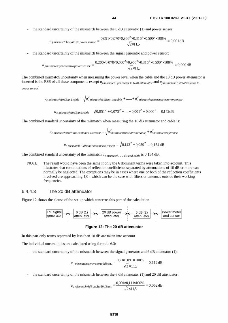
ETSI
ETSI TR 100 028-1 V1.3.1 (2001-03)44
- the standard uncertainty of the mismatch between the 6 dB attenuator (1) and power sensor:
dB0,0015112
%10050003160966007000910 222
1.6: =×
×××××=,
,,,,,u sensorpowertoattdBj mismatch
- the standard uncertainty of the mismatch between the signal generator and power sensor:
dB0,0005112
%100500031609660500007002000 2222
: =×
××××××=,
,,,,,,u sensorpowertogeneratorj mismatch
The combined mismatch uncertainty when measuring the power level when the cable and the 10 dB power attenuator isinserted is the RSS of all these components except uj mismatch: generator to 6 dB attenuator and uj mismatch: 6 dB attenuator to
power sensor:
2:.
21.6:10: ...... sensorpowertogeneratormismatchjcabletoattdBmismatchjcableanddBc mismatch uuu ++=
dB142,0000,0001,0....073,0051,0 222210: =++++=cableanddBc mismatchu
The combined standard uncertainty of the mismatch when measuring the 10 dB attenuator and cable is:
2:.
210:10: referencemismatchccableandattdBmismatchctmeasuremencableanddBc mismatch uuu +=
dB0,154059,0142,0 2210: =+=tmeasuremencableanddBc mismatchu
The combined standard uncertainty of the mismatch uc mismatch: 10 dB and cable is 0,154 dB.
NOTE: The result would have been the same if only the 6 dominant terms were taken into account. Thisillustrates that combinations of reflection coefficients separated by attenuations of 10 dB or more cannormally be neglected. The exceptions may be in cases where one or both of the reflection coefficientsinvolved are approaching 1,0 - which can be the case with filters or antennas outside their workingfrequencies.
6.4.4.3 The 20 dB attenuator
Figure 12 shows the clause of the set-up which concerns this part of the calculation.
Power meterand sensor
6 dB (1)attenuator
RF signalgenerator
20 dB powerattenuator
6 dB (2)attenuator
Figure 12: The 20 dB attenuator
In this part only terms separated by less than 10 dB are taken into account.
The individual uncertainties are calculated using formula 6.3:
- the standard uncertainty of the mismatch between the signal generator and 6 dB attenuator (1):
dB0,1125112
%100091020.6: =
×××=
,
,,u attdBtogeneratorj mismatch
- the standard uncertainty of the mismatch between the 6 dB attenuator (1) and 20 dB attenuator:
dB0,0625112
%10011100910.201.6: =
×××=,
,,u attdBtoattdBj mismatch
ETSI
ETSI TR 100 028-1 V1.3.1 (2001-03)45
- the standard uncertainty of the mismatch between the 20 dB attenuator and 6 dB attenuator (2):
dB0,0625112
%100091011102.6.20: =
×××=,
,,u attdBtoattdBj mismatch
- the standard uncertainty of the mismatch between the 6 dB attenuator (2) and power sensor:
dB0,0395112
%1000700910.6: =
×××=,
,,u sensorpowertoattdBj mismatch
- the standard uncertainty of the mismatch between the signal generator and 20 dB attenuator:
dB0,0345112
%100500011102000 2
.20: =×
×××=,
,,,u attdBtogeneraorj mismatch
- the standard uncertainty of the mismatch between the 20 dB attenuator and power sensor:
dB0,0125112
%100500007001110 2
.20: =×
×××=,
,,,u sensorpowertoattdBj mismatch
The rest of the combinations are not taken into account because the insertion losses between them are so high, that thevalues are negligible:
- 6 dB attenuator (1) and 6 dB attenuator (2);
- signal generator and 6 dB attenuator (2);
- 6 dB attenuator (1) and measuring receiver;
- signal generator and measuring receiver.
The combined standard uncertainty of the mismatch when measuring the attenuation of the 20 dB attenuator is the RSSof these 4 individual standard uncertainty values:
dB095,0012,0034,0062,0062,0 222220: =+++=dBj mismatchu
The combined standard uncertainty of the mismatch involved in the 20 dB attenuator measurement is:
2:
220:20: referencec mismatchdBc mismatchtmeasuremendBc mismatch uuu +=
dB0,11205900950 2220: =+= ,,u tmeasuremendBc mismatch
NOTE: If the two 6 dB attenuators had not been inserted, the result would have been 0,265 dB.
6.4.4.4 Instrumentation
Linearity of the measuring receiver is ±0,04 dB (from manufacturers data) as nothing is said about the distribution, arectangular distribution in logs is assumed and the standard uncertainty is calculated:
standard uncertainty dB0,0233
040 == ,u linearityj receiver

ETSI
ETSI TR 100 028-1 V1.3.1 (2001-03)46
6.4.4.5 Power and temperature influences
Temperature influence: 0,0001 dB/degree (from manufacturers data), which is negligible, the power influence for the10 dB attenuator is 0,0001 dB/dB × Watt (from manufacturers data) which gives 0,0001 × 25 × 10 = 0,025 dB asnothing is said about the distribution, a rectangular distribution in logs is assumed and the standard uncertainty iscalculated:
dB0,0143
025010 == ,
u dBfluenceinj power
The power influence for the 20 dB attenuator is 0,001 dB/dB × Watt (from manufacturers data) which gives0,001 × 2,5 × 20 = 0,05 dB as nothing is said about the distribution, a rectangular distribution in logs is assumed and thestandard uncertainty is calculated:
dB0,0283
050020 == ,
u dBnfluenceij power
6.4.4.6 Collecting terms
10 dB attenuator and cabling network uncertainty:
210
2210 dBnfluenceij powerlinearityj receiverc mismatchcableandattenuatordBc uuuu ++=
dB0,156014,0023,0154,0 22210 =++=cableandattenuatordBcu
20 dB attenuator and cabling network uncertainty:
220
2220 dBnfluenceij powerlinearityj receiverc mismatchattenuatordBc uuuu ++=
dB0,122028,004,0112,0 22220 =++=attenuatordBcu
The combined standard uncertainty of the attenuator and cabling network uncertainty:
220
210 attenuatordBccableandattenuatordBccablingandionc attenuat uuu +=
dB0,201122,0160,0 22 =+=cablingandionc attenuatu
6.4.5 Mismatch during measurement
Standing wave ratios involved in the power measurement:
- EUT: ρ = 0,500;
- Power sensor: VSWR ≤ 1,15 ρ = 0,070;
- 10 dB power attenuator: VSWR ≤ 1,3 ρ = 0,130;
- 20 dB attenuator: VSWR ≤ 1,25 ρ = 0,111;
- Cable: VSWR ≤ 1,2 ρ = 0,091.

ETSI
ETSI TR 100 028-1 V1.3.1 (2001-03)47
The mismatch uncertainties are calculated using formula 6.3 for the individual mismatch uncertainties between:
- the standard uncertainty of the mismatch between the EUT and cable:
dB0,1125112
%10009102000: =
×××=,
,,u cabletoEUTj mismatch
- the standard uncertainty of the mismatch between the cable and 10 dB power attenuator:
dB0,0735112
%10013000910.10: =
×××
=,
,,u attdBtocablej mismatch
- the standard uncertainty of the mismatch between the 10 dB power attenuator and 20 dB attenuator:
dB0,0895112
%10011101300.20.10: =
×××=,
,,u attdBtoattdBj mismatch
- the standard uncertainty of the mismatch between the 20 dB attenuator and power sensor:
dB0,0485112
%10007001110.20: =
×××=,
,,u sensorpowertoattdBj mismatch
- the standard uncertainty of the mismatch between the EUT and 10 dB power attenuator:
dB0,1495112
%100966013002000 2
.10: =×
×××=
,
,,,u attdBtoEUTj mismatch
- the standard uncertainty of the mismatch between the cable and 20 dB attenuator:
dB0,0585112
%1003160966011100910 22
.20: =×
××××=,
,,,,u attdBtocablej mismatch
- the standard uncertainty of the mismatch between the EUT and 20 dB attenuator:
dB0,0135112
%1003160966011102000 22
.20: =×
××××=,
,,,,u attdBtoEUTj mismatch
The rest of the combinations:
- 10 dB attenuator to power sensor;
- cable to power sensor;
- EUT to power sensor;
are neglected. The combined standard uncertainty of the mismatch during the measurement is the RSS of the individualcomponents:
dB0,2320130058,014900480089007301120 2222222 =++++++= ,,,,,,uc mismatch
In the case where all contributions are considered as independent.
6.4.6 Influence quantities
The two influence quantities involved in the measurement are ambient temperature and supply voltage.
Temperature uncertainty: ±1,0°C.
Supply voltage uncertainty: ±0,1 V.

ETSI
ETSI TR 100 028-1 V1.3.1 (2001-03)48
Uncertainty caused by the temperature uncertainty: Dependency function (from ETR 028 [15], part 2, annex F,table F.1): Mean value 4 %/°C and standard deviation: 1,2 %/°C.
Standard uncertainty of the power uncertainty caused by ambient temperature uncertainty (formula 5.2; see alsoannex D, clause D.4.2.1 in part 2).
( ) dB0,10521043
01
023
1 222
/ =+= ,,,
,u etemperaturj power
Uncertainty caused by supply voltage uncertainty: Dependency function (from ETR 028 [15]: part 2: annex F:table F.1): Mean: 10 %/V and standard deviation: 3 %/V power, Standard uncertainty of the power uncertainty causedby power supply voltage uncertainty (formula 5.2; see also annex D, clause D.4.2.1 in part 2).
( ) dB0,0263103
10
023
1 222
/ =+= ,
,u voltagej power
dB0,10802601050 222/
2/ =+=+= ,,uuu voltagepowerjetemperaturpowerjnfluenceic
6.4.7 Random
The measurement was repeated 9 times The following results were obtained (before correcting for cabling andattenuator network insertion loss):
- 21,8 mW, 22,8 mW, 23,0 mW, 22,5 mW, 22,1 mW, 22,7 mW, 21,7 mW, 22,3 mW, 22,7 mW.
The two sums X and Y are calculated:
- X = the sum of the measured values = 201,6 mW;
- Y = the sum of the squares of the measured values = 4517,5 mW2;
- =−
−=
−
−=
199
620154517
1
22 ,,
nn
XY
uc random 0,456 mW (formula 5.5);
- Mean value = 22,4 mW.
As the result is obtained as the mean value of 9 measurements the standard uncertainty (converted to dB by divisionwith 23,0) of the random uncertainty is:
dB0,089023
100
422
4560 =×=,,
,uc random
NOTE: It is important to try and identify whether this value corresponds to the effect of other uncertainties,already taken into account in the calculations (e.g. uncertainties due to the instrumentation), or whetherthis corresponds to a genuine contribution (in which cas it has to be combined with all the othercontributions)… obviously, there are uncertainties in the measurements, so it has to be expected thatperforming the same measurement a number of times may provide a set of different results.
6.4.8 Expanded uncertainty
The combined standard uncertainty for the carrier power measurement is the RSS of all the calculated part standarduncertainties:
22222c randomfluencec inc mismatchcablingandionc attenuatsensorandc meterpowercarrierc uuuuuu ++++=
dB0,34408901080232020100660 22222 =++++= ,,,,,u powercarrierc
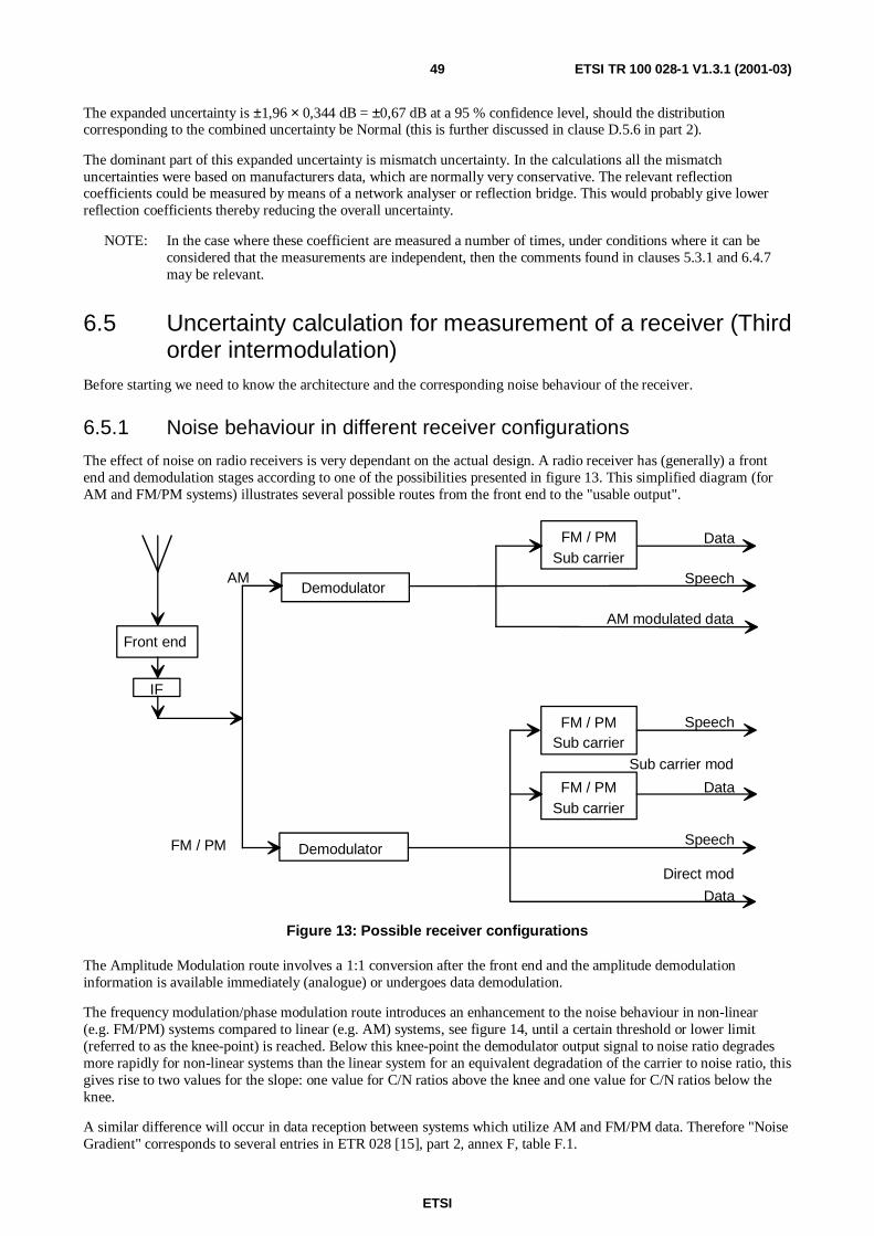
ETSI
ETSI TR 100 028-1 V1.3.1 (2001-03)49
The expanded uncertainty is ±1,96 × 0,344 dB = ±0,67 dB at a 95 % confidence level, should the distributioncorresponding to the combined uncertainty be Normal (this is further discussed in clause D.5.6 in part 2).
The dominant part of this expanded uncertainty is mismatch uncertainty. In the calculations all the mismatchuncertainties were based on manufacturers data, which are normally very conservative. The relevant reflectioncoefficients could be measured by means of a network analyser or reflection bridge. This would probably give lowerreflection coefficients thereby reducing the overall uncertainty.
NOTE: In the case where these coefficient are measured a number of times, under conditions where it can beconsidered that the measurements are independent, then the comments found in clauses 5.3.1 and 6.4.7may be relevant.
6.5 Uncertainty calculation for measurement of a receiver (Thirdorder intermodulation)
Before starting we need to know the architecture and the corresponding noise behaviour of the receiver.
6.5.1 Noise behaviour in different receiver configurations
The effect of noise on radio receivers is very dependant on the actual design. A radio receiver has (generally) a frontend and demodulation stages according to one of the possibilities presented in figure 13. This simplified diagram (forAM and FM/PM systems) illustrates several possible routes from the front end to the "usable output".
Front end
IF
Demodulator
Demodulator
FM / PMSub carrier
FM / PMSub carrier
FM / PMSub carrier
AM modulated data
Speech
Data
Speech
Data
Speech
Data
Sub carrier mod
Direct mod
FM / PM
AM
Figure 13: Possible receiver configurations
The Amplitude Modulation route involves a 1:1 conversion after the front end and the amplitude demodulationinformation is available immediately (analogue) or undergoes data demodulation.
The frequency modulation/phase modulation route introduces an enhancement to the noise behaviour in non-linear(e.g. FM/PM) systems compared to linear (e.g. AM) systems, see figure 14, until a certain threshold or lower limit(referred to as the knee-point) is reached. Below this knee-point the demodulator output signal to noise ratio degradesmore rapidly for non-linear systems than the linear system for an equivalent degradation of the carrier to noise ratio, thisgives rise to two values for the slope: one value for C/N ratios above the knee and one value for C/N ratios below theknee.
A similar difference will occur in data reception between systems which utilize AM and FM/PM data. Therefore "NoiseGradient" corresponds to several entries in ETR 028 [15], part 2, annex F, table F.1.

ETSI
ETSI TR 100 028-1 V1.3.1 (2001-03)50
Knee point
Linea
r syste
m(A
M)
Non-lin
ear sy
stem
(FM/P
M)
Better >
Bet
ter
>S
/N
C/N
Figure 14: Noise behaviour in receivers
6.5.2 Sensitivity measurement
The sensitivity of a receiver is usually measured as the input RF signal level which produces a specific outputperformance which is a function of the base band signal-to-noise ratio in the receiver.
This is done by adjusting the RF level of the input signal at the RF input of the receiver.
What is actually done is that the RF signal-to-noise ratio at the input of the receiver is adjusted to produce a specifiedsignal-to-noise ratio dependant behaviour at the output of the receiver, i.e. SINAD, BER, or message acceptance.
An error in the measurement of the output performance will cause a mis adjustment of the RF level and thereby theresult.
In other words any uncertainty in the output performance is converted to signal-to-noise ratio uncertainty at the input ofthe receiver. As the noise does not change it causes an uncertainty in the adjusted level.
For an analogue receiver, the dependency function to transform the SINAD uncertainty to the RF input level uncertaintyis the slope of the noise function described above in clause 6.5.1 and depends on the type of carrier modulation.
The dependency function involved when measuring the sensitivity of an FM/PM receiver is the noise behaviour usuallybelow the knee-point for a non-linear system, in particular in the case of data equipment. This function also affects theuncertainty when measuring sensitivity of an FM/PM based data equipment.
This dependency function has been empirically derived at 0,375 dB RF i/p level / dB SINAD associated with a standarduncertainty of 0,075 dB RF i/p level / dB SINAD and is one of the values stated in ETR 028 [15], part 2, annex F, table F.1.
If the receiver is for data the output performance is a specified BER. BER measurements are covered by clause 6.6.
In some standards the sensitivity is measured as the output performance at a specified input level. In this case thedependency functions converting input level uncertainty to output performance uncertainty are the inverse of thefunctions previously described.

ETSI
ETSI TR 100 028-1 V1.3.1 (2001-03)51
6.5.3 Interference immunity measurements
Interference immunity (i.e. co-channel rejection, adjacent channel rejection) is measured by adjusting the RF level ofthe wanted signal to a specified value. Then the RF level of the interfering signal is adjusted to produce a specifiedperformance at the output of the receiver.
The interfering signal is normally modulated. Therefor for measurement uncertainty purposes it can be regarded aswhite noise in the receiving channel.
The uncertainty analysis is therefor covered by clause 6.5.2.
6.5.4 Blocking and spurious response measurements
These measurements are similar to interference immunity measurements except that the unwanted signal is withoutmodulation.
Even though the unwanted signal (or the derived signal in the receive channel caused by the unwanted signal) can not inevery case be regarded as white noise, the present document does not distinguish. The same dependency functions areused.
6.5.5 Third order intermodulation
When two unwanted signals X and Y occur at frequency distance d(X) and 2d(Y) from the receiving channel a disturbingsignal Z is generated in the receiving channel due to non linearities in filters, amplifiers and mixers.
The physical mechanism behind the intermodulation is the third order component of the non-linearity of the receiver:
K × X3
When two signals - X and Y - are subject to that function, the resulting function will be:
- K(X + Y)3 = K(X3 + Y3 + 3X2Y + 3XY2), where the component Z = 3X2Y is the disturbing intermodulation productin the receiving channel.
If X is a signal Ix sin(2π(fo+d)t) and Y is a signal Iy sin(2π(fo+2d)t), the component:
- Z = K × 3X2Y will generate a signal having the frequency fo and the amplitude K × 3Ix2Iy.
(A similar signal Z' = 3XY2 is generated on the other side of the two signals X and Y, as shown in figure 15).
The predominant function is a third order function:
Iz = Ic + 2Ix + Iy (6.4)
where lz is the level of the intermodulation product Z, Ic is a constant, Ix and Iy are the levels of X and Y. All terms arelogarithmic.
6.5.5.1 Measurement of third order intermodulation
The measurement is normally carried out as follows.
Three signal generators are connected to the input of the EUT.
Generator 1 is adjusted to a specified level at the receiving frequency fo (the wanted signal W).
Generator 2 is adjusted to frequency fo+ δ (unwanted signal X) and generator 3 is adjusted to frequency fo+ 2δ(unwanted signal Y). The level of X and Y (Ix and Iy) are maintained equal during the measurement.
Ix and Iy are increased to level A which causes a specified degradation of AF output signal (SINAD) or a specific bit
error ratio (BER) or a specific acceptance ratio for messages.
Both the SINAD, BER and message acceptance ratio are a function of the signal-to-noise ratio in the receiving channel.
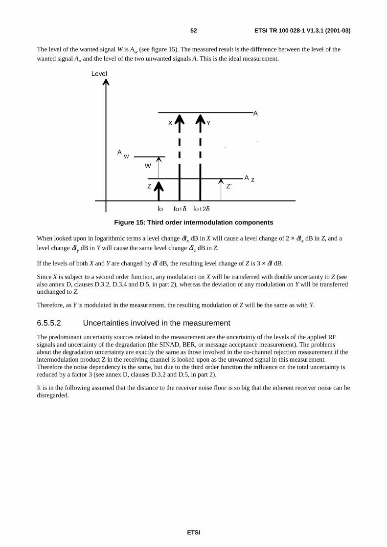
ETSI
ETSI TR 100 028-1 V1.3.1 (2001-03)52
The level of the wanted signal W is Aw (see figure 15). The measured result is the difference between the level of the
wanted signal Aw and the level of the two unwanted signals A. This is the ideal measurement.
A
A zZ
X Y
Z'
Level
Aw
W
fo fo+δ fo+2δ
Figure 15: Third order intermodulation components
When looked upon in logarithmic terms a level change δIx dB in X will cause a level change of 2 × δIx dB in Z, and a
level change δIy dB in Y will cause the same level change δIz dB in Z.
If the levels of both X and Y are changed by δI dB, the resulting level change of Z is 3 × δI dB.
Since X is subject to a second order function, any modulation on X will be transferred with double uncertainty to Z (seealso annex D, clauses D.3.2, D.3.4 and D.5, in part 2), whereas the deviation of any modulation on Y will be transferredunchanged to Z.
Therefore, as Y is modulated in the measurement, the resulting modulation of Z will be the same as with Y.
6.5.5.2 Uncertainties involved in the measurement
The predominant uncertainty sources related to the measurement are the uncertainty of the levels of the applied RFsignals and uncertainty of the degradation (the SINAD, BER, or message acceptance measurement). The problemsabout the degradation uncertainty are exactly the same as those involved in the co-channel rejection measurement if theintermodulation product Z in the receiving channel is looked upon as the unwanted signal in this measurement.Therefore the noise dependency is the same, but due to the third order function the influence on the total uncertainty isreduced by a factor 3 (see annex D, clauses D.3.2 and D.5, in part 2).
It is in the following assumed that the distance to the receiver noise floor is so big that the inherent receiver noise can bedisregarded.

ETSI
ETSI TR 100 028-1 V1.3.1 (2001-03)53
6.5.5.2.1 Signal level uncertainty of the two unwanted signals
A is the assumed level of the two unwanted signals (the indication of the two unwanted signal generators corrected formatching network attenuations):
- Ax is the true level of X and Ay is the true level of Y. (Ax is A+δx and Ay is A+δy) see figure 16;
- Az is the level of Z (the same as in the ideal measurement).
A
A z
Ax
Ay
Z
X
Y
Z'
Level
δX
δY
A w
W
fo fo+δ fo+2δ
Figure 16: Level uncertainty of two unwanted signals
If Ax and Ay were known the correct measuring result would be obtained by adjusting the two unwanted signals to the
level At (true value) which still caused the level Az of Z.
If there is an error δx of the level of signal X, the error of the level of the intermodulation product will be 2 × δx (seealso annex D, clauses D.3 and D.5, in part 2); to obtain the wanted signal-to-noise ratio the two unwanted levels must bereduced by 2 × δx/3.
In other words the dependency function of generator X is 2/3.
In the same way if there is an error δy of the level of signal Y, the error of the level of the intermodulation product willbe δy; to obtain the wanted signal-to-noise ratio the two unwanted signals must be reduced by δy/3.
In other words the dependency function of generator Y is 1/3.
When looking at the problem in linear terms, the dependency functions are valid for small values of δx and δy due to thefact that the higher order components of the third order function can be neglected.
δx and δy are the relative RF level uncertainties at the input of the EUT. They are combinations of signal generator leveluncertainty, matching network attenuation uncertainty and mismatch uncertainties at the inputs and the output of thematching network.
The standard uncertainties of the levels of X and Y are uj x and uj y.
The standard uncertainty uj unwanted signals related to the uncertainty caused by level uncertainty of the two unwantedsignals is thus (see also clause D.3.2.3 of annex D, in part 2):
j yj xsignalsj unwanted u+u=u
3
1
3
2 22
(6.5)

ETSI
ETSI TR 100 028-1 V1.3.1 (2001-03)54
6.5.5.2.2 Signal level uncertainty of the wanted signal
Under the assumption that equal change of both the level of the wanted signal and the intermodulation product willcause no change of the SINAD, (or the BER, or the message acceptance) the error contribution from the uncertainty ofthe level of the wanted signal can be calculated.
If there is an error δw on the wanted signal, the two unwanted signal levels must be adjusted by 1/3 × δw to obtain thewanted signal-to-noise ratio. The dependency function of generator W is therefore 1/3 and assuming the same types ofuncertainties as previously the standard uncertainty, uj wanted signal, is (see clause D.3.2.3 of annex D, in part 2):
signalsj unwantedsignalj wanted u=u
3
1(6.6)
6.5.5.3 Analogue speech (SINAD) measurement uncertainty
Sensitivity is normally stated as an RF input level in conducted measurements.
For analogue systems this is stated as at a specified SINAD value.
For an analogue receiver, the dependency function to transform the SINAD uncertainty to the RF input level uncertaintyis the slope of the noise function described above in clause 6.5.1 and depends on the type of carrier modulation.
The dependency function involved when measuring the sensitivity of an FM/PM receiver is the noise behaviour usuallybelow the knee-point for a non-linear system, in particular in the case of data equipment. This function also affects theuncertainty when measuring sensitivity of an FM/PM based data equipment.
This dependency function has been empirically derived at 0,375 dB RF i/p level / dB SINAD associated with a standarduncertainty of 0,075 dB RF i/p level / dB SINAD and is one of the values stated in ETR 028 [15], part 2, annex F, table F.1.
The SINAD measurement uncertainty also contributes to the total measurement uncertainty.
If the receiver is working beyond the demodulator knee point any SINAD uncertainty corresponds to an equaluncertainty (in dB) of the signal-to-noise ratio.
If the receiver is working below the knee point the corresponding uncertainty of the signal-to-noise ratio will be in theorder of 1/3 times the SINAD uncertainty (according to ETR 028 [15], part 2, annex F, table F.1).
Any signal-to-noise ratio uncertainty causes 1/3 times that uncertainty in the combined uncertainty: the unwanted signallevels must be adjusted by 1/3 of the signal-to-noise ratio error to obtain the correct value.
Therefore if the receiver is working above the knee point the SINAD dependency function is 1/3, and if the receiver isworking below the knee point the dependency function is in the order of 1/9.
6.5.5.4 BER and message acceptance measurement uncertainty
Any BER (or message acceptance) uncertainty will influence the total uncertainty by the inverse of the slope of theappropriate BER function at the actual signal-to-noise ratio.
As the BER function is very steep, the resulting dependency function is small, and it is sufficient to use the differentialcoefficient as an approximation.
If the signalling is on a sub carrier, the relation between the signal-to-noise ratio of the sub carrier must be dealt with inthe same way as with other receiver measurements. See clause 6.6.3.

ETSI
ETSI TR 100 028-1 V1.3.1 (2001-03)55
6.5.5.5 Other methods of measuring third order intermodulation
Some test specifications specify other methods of measuring the intermodulation rejection.
The measured result is the SINAD, BER, or message acceptance at fixed test signal levels. This is the case with somedigital communication equipment like DECT and GSM.
In these measurements the uncertainty must be calculated in 3 steps:
1) the uncertainty of the resulting signal-to-noise ratio is calculated;
2) this uncertainty is then applied to the appropriate SINAD, BER, or message acceptance function;
3) and then combined with the measurement uncertainty of the SINAD, BER, or message acceptance measurement.
The uncertainty of the signal-to-noise ratio due to uncertainty of the level of the test signals is:
( ) 2222 j wj yj xj SNR uuu=u ++
This uncertainty is then transformed to the measured parameter.
If the measured value is a SINAD value and the receiver is working beyond the knee point the SINAD uncertainty isidentical, but if the receiver is working below the knee point the dependency function is in the order of 3,0.
If the measurand is a BER or a message acceptance, the dependency function is too non linear to be regarded as a firstorder function.
The total uncertainty must then be calculated as described in clause 6.6.4.3.
6.6 Uncertainty in measuring continuous bit streams
6.6.1 General
If an EUT is equipped with data facilities, the characteristic used to assess its performance is the Bit Error Ratio (BER).
The BER is the ratio of the number of bits in error to the total number of bits in a received signal and is a good measureof receiver performance in digital radio systems just as SINAD is a good measure of receiver performance in analogueradios. BER measurements, therefore, are used in a very similar way to SINAD measurements, particularly insensitivity and immunity measurements.
6.6.2 Statistics involved in the measurement
Data transmissions depend upon a received bit actually being that which was transmitted. As the level of the receivedsignal approaches the noise floor (and therefore the signal to noise ratio decreases), the probability of bit errors (and theBER) increases.
The first assumption for this statistical analysis of BER measurements is that each bit received (with or without error) isindependent of all other bits received. This is a reasonable assumption for measurements on radio equipment, usingbinary modulation, when measurements are carried out in steady state conditions. If, for instance, fading is introduced,it is not a reasonable assumption.
The measurement of BER is normally carried out by comparing the received data with that which was actuallytransmitted. The statistics involved in this measurement can be studied using the following population of stones: oneblack and (1/BER)-1 white stones. If a stone is taken randomly from this population, its colour recorded and the stonereplaced N times, the black stone ratio can be defined as the number of occurrences of black stones divided by N. Thisis equivalent to measuring BER.

ETSI
ETSI TR 100 028-1 V1.3.1 (2001-03)56
The statistical distribution for this measurement is the binomial distribution. This is valid for discrete events and givesthe probability that x samples out of the N stones sampled are black stones (or x bits out of N received bits are in error)given the BER:
( ) ( ) ( ) xNxx BERBER
!xNx!
N!P −−×
−= 1 (6.7)
The mean value of this distribution is BER × N and the standard deviation is:
( ) NBERBER ×−× 1 (6.8)
and for large values of N the shape of the distribution approximates a Gaussian distribution.
Normalizing the mean value and standard uncertainty (by dividing by N) gives:
Mean value = BER (6.9)
( )N
BERBERu BERj
−= 1(6.10)
From these two formulas it is easy to see that the larger number of bits, the smaller the random uncertainty, and therelation between number of bits and uncertainty is the same as for random uncertainty in general. By means offormula 6.11 it is possible to calculate the number of bits needed to be within a specific uncertainty.
For example: A BER in the region of 0,01 is to be measured.
a) If the standard uncertainty, due to the random behaviour discussed above, is to be 0,001, then the number of bitsto be compared, N, in order to fulfil this demand is calculated from the rearranged formula (6.11).
( )9900
0010
990010122
=×=−=,
,,
u
BERBERN
jBER
b) If the number of bits compared, N, is defined, e.g. 2 500 then the standard uncertainty is given directly byformula (6.11).
( )0020
2500
0101010,
,,u BERj =−=
As stated earlier the binomial distribution can be approximated by a Normal distribution. This is not true when the BERis so small that only a few bit errors (< 10) are detected within a number of bits. In this case the binomial distribution isskewed as the p (BER < 0) = 0.
Another problem that occurs when only few bit errors are detected, and the statistical uncertainty is the dominantuncertainty (which does not happen in PMR measurements, but it does, due to the method, occur in DECT and GSMtests) is that the distribution of the true value about the measured value can be significantly different from an assumedNormal distribution.
6.6.3 Calculation of uncertainty limits when the distribution characterizingthe combined standard uncertainty cannot be assumed to be aNormal distribution
In the calculations of uncertainty there is usually no distinction between the distribution of a measured value about thetrue value, and the distribution of the true value about a measured value. The assumption is that they are identical.
This is true in the cases where the standard uncertainty for the distribution of the measured value about the true value isindependent of the true value - which usually is the case. But if the standard uncertainty is a function of the true value ofthe measurand (not the measured value), the resulting distribution of the measurement uncertainty will not be a Normaldistribution even if the measured value about the true value is.
This is illustrated by the following (exaggerated) example.

ETSI
ETSI TR 100 028-1 V1.3.1 (2001-03)57
A DC voltage is to be measured. We assume that there is only one uncertainty contribution which comes from thevoltmeter used for the measurement.
In the manufacturers data sheet for the voltmeter it is stated that the measured value is within ±25 % of the true value.
If the true value is 1,00 V then the measured value lies between 0,75 V and 1,25 V. However, if the measured value is0,75 V and the true value is still 1,00 V corresponding to 1,3333 times the measured value. Similarly, If the measuredvalue is 1,25 V and the true value is still 1,0 V this corresponds to 0,8 times the measured value.
Therefore the limits are asymmetric for the true value about the measured value (-20 % and +33,33 %).
When looking at the standard deviations, the error introduced is small. In the previous example the standard deviationof the measured value about the true value is 14,43 %. The standard deviation of the related true value about themeasured value is 15,36 %. As the difference is small, and the distribution of the measured value about the true value isbased on an assumption anyway, the present document suggests that it can be used directly.
NOTE: The average value, however, is no longer zero, but in this case is approximately 4,4 %.
Alternatively, also in this example, xt is the true value and xm is the measured value. Any parameter printed in square
brackets, e.g. [xm], is considered to be constant.
The distribution of the measured value xm about the true value xt is given by the function p (xm, [xt]).
Based on this function the distribution p1 (xt, [xm]) of the true value xt about the measured value xm can be derived.
The intermediate function is p (xt, [xm]) which is the same as the previous; the only difference being that xt is the
variable and xm is held constant. This function is not a probability distribution as the integral from -∞ to +∞ is not unity.To be converted to the probability function p1 (xt, [xm]) it must be normalized. Therefore:
[ ]( ) [ ]( )
[ ]( )∫∞
∞−
=
dxxx,p
x,xpx,xp
m
mtmt1 (6.11)
As this distribution is not Normal, the uncertainty limits must be found by other means than by multiplication with acoverage factor from Student's t-distribution. How the actual limits are calculated in practise depends on the actualdistribution.
An example: If the true BER of a radio is 5 × 10⁻⁶ and the BER is measured over 106 bits, the probability of detecting0 bits is 0,674 %. On the other hand if the BER in a measurement is measured as 5 × 10⁻⁶ the true value cannot be 0.
If the uncertainty calculations are based on the assumption of a Gaussian distribution, the lower uncertainty limitbecomes negative (which of course doesn't reflect reality, and provides the evidence that not all distributions areNormal!).
The standard uncertainty based on the measured value 3,0 × 10⁻⁶:
( ) 66
66
101,7310
100311003 −−−
×=×−×
=,,
u j
The expanded uncertainty is ±1,96 × 1,73 × 10-6 = ±3,39 × 10⁻⁶ at a 95 % confidence level.
The correct distribution p1 (xt) is the continuous function in figure 17.
NOTE: The true value is not BER, but number of bit errors, where BER= (bit errors/number of bits tested)). Thebinomial function p (xm) based on the true value = 3 bit errors (corresponding to BER = 3 × 10⁻⁶) is thediscrete function shown.

ETSI
ETSI TR 100 028-1 V1.3.1 (2001-03)58
The distribution p (xt) (based on the binomial distribution with 3 bit errors and 106 bits tested):
( )( )
%xx
kxp ttt
310
6
3
6
6
101
10100
−
−×
××= where ( )
176
610671
3103
10 ×=−×
= ,!!
!k
The integral from -∞ to +∞ of p (xt) is very close to 1. Therefore p (xt) is a good approximation to the correct
distribution p1 (xt).
By means of numerical methods the 95 % error limits are found to be +5,73 and -1,91 corresponding to +5,73 × 10⁻⁶ and-1,91 × 10⁻⁶.
Figure 17 shows the discrete distribution giving the probabilities of measuring from 0 to 14 bit errors when the truevalue is 3 bit errors corresponding to BER = 3 × 10⁻⁶, and the continuous distribution giving the probability function forthe true value when the measured value is 3 bit errors corresponding to BER = 3 × 10⁻⁶.
05
1015
2025
%
bit errors0 1 2 3 4 5 6 7 8 9 10 11 12 13 14
p (x )1 t
Figure 17: BER uncertainty
6.6.4 BER dependency functions
As in SINAD measurements, the BER of a receiver is a function of the signal to noise ratio of the RF signal at the inputof the receiver.
Several modulation and demodulation techniques are used in data communication and the dependency functions arerelated to these techniques.
This clause covers the following types of modulation:
- coherent modulation/demodulation of the RF signal;
- non coherent modulation/demodulation of the RF signal;
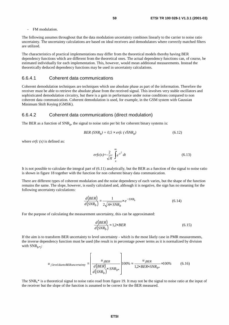
ETSI
ETSI TR 100 028-1 V1.3.1 (2001-03)59
- FM modulation.
The following assumes throughout that the data modulation uncertainty combines linearly to the carrier to noise ratiouncertainty. The uncertainty calculations are based on ideal receivers and demodulators where correctly matched filtersare utilized.
The characteristics of practical implementations may differ from the theoretical models thereby having BERdependency functions which are different from the theoretical ones. The actual dependency functions can, of course, beestimated individually for each implementation. This, however, would mean additional measurements. Instead thetheoretically deduced dependency functions may be used in uncertainty calculations.
6.6.4.1 Coherent data communications
Coherent demodulation techniques are techniques which use absolute phase as part of the information. Therefore thereceiver must be able to retrieve the absolute phase from the received signal. This involves very stable oscillators andsophisticated demodulation circuitry, but there is a gain in performance under noise conditions compared to noncoherent data communication. Coherent demodulation is used, for example, in the GSM system with GaussianMinimum Shift Keying (GMSK).
6.6.4.2 Coherent data communications (direct modulation)
The BER as a function of SNRb, the signal to noise ratio per bit for coherent binary systems is:
BER (SNRb) = 0,5 × erfc (√SNRb) (6.12)
where erfc (x) is defined as:
dteerfc(x)= -t
x
22∫∞
π(6.13)
It is not possible to calculate the integral part of (6.11) analytically, but the BER as a function of the signal to noise ratiois shown in figure 18 together with the function for non coherent binary data communication.
There are different types of coherent modulation and the noise dependency of each varies, but the shape of the functionremains the same. The slope, however, is easily calculated and, although it is negative, the sign has no meaning for thefollowing uncertainty calculations:
( )( )
bSNR
bbe
SNRSNRd
BERd −××
=π2
1(6.14)
For the purpose of calculating the measurement uncertainty, this can be approximated:
( )( ) BER,SNRd
BERd
b×≈ 21 (6.15)
If the aim is to transform BER uncertainty to level uncertainty - which is the most likely case in PMR measurements,the inverse dependency function must be used (the result is in percentage power terms as it is normalized by divisionwith SNRb*):
( )( )
%SNRBER,
u%
SNRSNRd
BERd
uu
b
jBER
bb
jBERntyuncertaiBERtoduej level 100
21100
**
×××
≈
×= (6.16)
The SNRb* is a theoretical signal to noise ratio read from figure 19. It may not be the signal to noise ratio at the input ofthe receiver but the slope of the function is assumed to be correct for the BER measured.

ETSI
ETSI TR 100 028-1 V1.3.1 (2001-03)60
For example: The sensitivity of a receiver is measured. The RF input level to the receiver is adjusted to obtain a BER of10-2. The measured result is the RF level giving this BER. The BER is measured over a series of 25 000 bits. Theresulting BER uncertainty is then calculated using formula (6.11):
( ) 41029625000
0101010 −×=−
= ,,,
u j BER
The uncertainty of the RF signal at the input is 0,7 dB (uj). The signal to noise ratio giving this BER is then read from
figure 18: SNRb*(0,01) = 2,7 and the dependency function at this level is:
( )( )( )
22 1021101212172 −− ×=××=×= ,,BER,
SNRd
,BERd
b
The BER uncertainty is then transformed to level uncertainty using formula (6.16):
power%1,951007,21021
102962
4=×
××
×=
−
−%
,
,u j level dB0,085dB
023
951 =≈,
,
....085070 22 ++= ,,u levelj RF
There is an additional uncertainty component due to resolution of the readout of the measured BER. If the RF inputlevel has been adjusted to give a reading of 0,01 and the resolution of the BER meter is 0,001 the correct lies between0,0095 and 0,0105 with equal probability.
The standard deviation is therefore
43
108923
1050 −−
×=×= ,,
u lutionj BER reso
This standard deviation is then by means of formula 6.16 converted to level uncertainty:
%SNR
)d(SNR
d(BER)
uu
bb
lutionj BER resoesolutione to BER rj level du 100×
×=
dB,dB,
,%,%
,,,
,u esolutione to BER rj level du 0040
023
08900890100
7201021
102890 4=≈=×
×××=
−
The total uncertainty of the sensitivity level is then:
dB71,07,0004,0085,0 222222 =++=+= jresolutionBERtodueleveljleveljlevelc RF uuuu
As can be seen the BER statistical uncertainty and the BER resolution only plays a miner role.
6.6.4.3 Coherent data communications (sub carrier modulation)
If a sub carrier frequency modulation is used in the data communication the functions related to direct coherent datacommunication apply, but in this case they give the relationship between BER and the signal to noise of the sub carrier.To be able to transform BER uncertainty to RF input level uncertainty the relationship between the sub carrier signal tonoise ratio and the RF carrier signal to noise ratio must be calculated.
If the BER is measured at a RF level much higher than the sensitivity this relation is assumed to be 1:1 as described inclause 6.5.
In FM systems, if the BER is measured in the sensitivity region (below the knee point) the relationship as for analoguereceivers is assumed and the same value taken from ETR 028 [15], part 2, annex F, table F.1, 0,375 dB RF i/p
level/dB SINAD and standard uncertainty 0,075 dB RF i/p level/dB SINAD. (see clause 6.5).

ETSI
ETSI TR 100 028-1 V1.3.1 (2001-03)61
EXAMPLE: The sensitivity of an FM receiver is measured. The RF input level to the receiver is adjusted toobtain a BER of 10-2. The measured result is the RF level giving this BER. The BER is measuredover a series of 2 500 bits. The uncertainty of the RF signal at the input is 0,5 dB (uj).
The resulting BER uncertainty is then calculated using formula (6.11):
( ) 310022500
0101010 −×=−
= ,,,
u j BER
The signal to noise ratio giving this BER is then read from figure 18: SNRb*(0,01) = 2,7. The dependency function at
this level is:
( )( )( )
22 10211001212172 −− ×=××=×= ,,,BER,
SNRd
,BERd
b
The BER uncertainty is then transformed to level (or SNRb) uncertainty using formula (6.4):
%6,17%100721021
10022
3=×
××
×=
−
−
,,
,u
bj SNR power, which is equal to (6,17/23,0) = 0,27 dB.
This uncertainty is then by means of formula (5.2) and the relationship taken from ETR 028 [15], part 2, annex F,table F.1 converted to RF input level uncertainty (as SINAD and SNRb is considered to be equivalent in this case). The
dependency function is: mean = 0,375 dB RF i/p level/dB SINAD and standard uncertainty 0,075 dB RF i/p level/dB SINAD.
( ) dB1020080380270 222 ,,,,u j level =+×= (formula 5.2)
This RF level uncertainty is then combined with the uncertainty of the level of the input signal to obtain the totaluncertainty of the sensitivity:
dB0,5110050 22 =+= ,,u ityj sensitiv
In this example the uncertainty due to meter resolution is assumed to be negligible.
6.6.4.4 Non coherent data communication
Non coherent modulation techniques disregard absolute phase information. Communications based on non coherentmodulation tend to be more sensitive to noise, and the techniques used may be much simpler. A typical non coherentdemodulation technique is used with FSK, where only the information of the frequency of the signal is required.
6.6.4.5 Non coherent data communications (direct modulation)
The BER as a function of the SNRb in this case is:
( ) 22
1bSNR
b eSNRBER−
= (6.17)
provided that the cross correlation coefficient ccross between the two frequencies defining the zeros and the ones is 0.
The cross correlation coefficient ccross of two FSK signals with frequency separation fδ and the bit time T is:
( )δ
δππ
fT
fTccross ××
××sin= (6.18)
It is assumed that the cross correlation coefficient for land mobile radio systems is so small that the formulas forccross = 0 apply, and as ccross is 0 the BER, as a function of the SNRb for non coherent modulation is shown inequation 6.15.

ETSI
ETSI TR 100 028-1 V1.3.1 (2001-03)62
The slope of the function (in fact the slope is negative, but the sign is of no interest for the uncertainty calculation). TheBER (SNRb) function for non coherent data communication is shown in figure 19.
The inverse function is:
SNRb (BER) = -2 × ln (2 × BER) (6.19)
From (6.17) the slope of SNRb (BER) is:
( )( ) BERBERd
SNRd b 2−= (6.20)
The slope of the function is the inverse of (6.18):
( )( ) 2
BER
SNRd
BERd
b= (6.21)
The SNRb can be calculated by means of formula (6.19) or read from the function shown in figure 19. If the aim is to
transform BER uncertainty to level uncertainty - which is generally the case in PMR measurements - formula (6.16) isused.
( )( ) *b
b
j BERj level
SNRSNRd
BERd
uu
×=
Before it can be combined with the other part uncertainties at the input of the receiver it must be transformed to linearvoltage terms.
EXAMPLE: The sensitivity of a receiver is measured. The RF input level to the receiver is adjusted to obtain aBER of 10-2. The measured result is the RF level giving this BER. The BER is measured over aseries of 2 500 bits. The uncertainty of the RF signal at the input is 0,6 dB (uj).
The resulting BER uncertainty is then calculated using formula (6.11):
3100022500
990010 −×=×
= ,,,
u j BER
The signal to noise ratio giving this BER is then calculated using formula (6.19).
SNRb (0,01) = -2 × ln (2 × 0,01) = 7,824
The dependency function at this level is (formula (6.21)):
( )( )( ) 01050
8247,,
SNRd
,BERd
b×=
The BER uncertainty is then transformed to level uncertainty using formula (6.16):
power%5,11%10082471050
100022
3=×
××
×=
−
−
,,
,u j level
which is equal to 5,11/23,0 dB = 0,22 dB (uj) in voltage terms. This RF level uncertainty is then combined with the restof the uncertainty contribution to give the combined standard uncertainty of the RF level.
( ) ( ) dB64022060 22 ,,,u levelc RF =+=
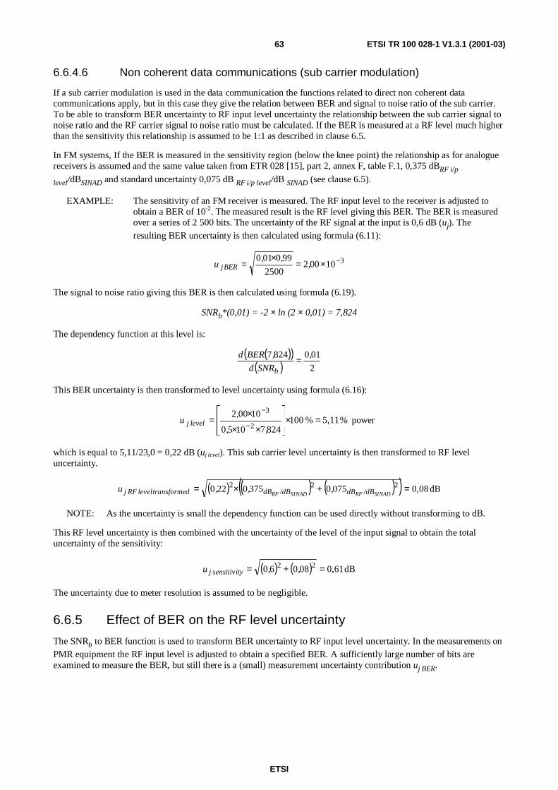
ETSI
ETSI TR 100 028-1 V1.3.1 (2001-03)63
6.6.4.6 Non coherent data communications (sub carrier modulation)
If a sub carrier modulation is used in the data communication the functions related to direct non coherent datacommunications apply, but in this case they give the relation between BER and signal to noise ratio of the sub carrier.To be able to transform BER uncertainty to RF input level uncertainty the relationship between the sub carrier signal tonoise ratio and the RF carrier signal to noise ratio must be calculated. If the BER is measured at a RF level much higherthan the sensitivity this relationship is assumed to be 1:1 as described in clause 6.5.
In FM systems, If the BER is measured in the sensitivity region (below the knee point) the relationship as for analoguereceivers is assumed and the same value taken from ETR 028 [15], part 2, annex F, table F.1, 0,375 dBRF i/p
level/dBSINAD and standard uncertainty 0,075 dB RF i/p level/dB SINAD (see clause 6.5).
EXAMPLE: The sensitivity of an FM receiver is measured. The RF input level to the receiver is adjusted toobtain a BER of 10-2. The measured result is the RF level giving this BER. The BER is measuredover a series of 2 500 bits. The uncertainty of the RF signal at the input is 0,6 dB (uj). Theresulting BER uncertainty is then calculated using formula (6.11):
3100022500
990010 −×=×
= ,,,
u BERj
The signal to noise ratio giving this BER is then calculated using formula (6.19).
SNRb*(0,01) = -2 × ln (2 × 0,01) = 7,824
The dependency function at this level is:
( )( )( ) 2
0108247 ,
SNRd
,BERd
b=
This BER uncertainty is then transformed to level uncertainty using formula (6.16):
power%5,11%10082471050
100022
3=×
××
×=
−
−
,,
,u j level
which is equal to 5,11/23,0 = 0,22 dB (uj level). This sub carrier level uncertainty is then transformed to RF leveluncertainty.
( ) ( ) ( )( ) dB0,0807503750220 222 =+×=SINADRFSINADRF /dBdB/dBdBdtransformelevelj RF ,,,u
NOTE: As the uncertainty is small the dependency function can be used directly without transforming to dB.
This RF level uncertainty is then combined with the uncertainty of the level of the input signal to obtain the totaluncertainty of the sensitivity:
( ) ( ) dB0,6108060 22 =+= ,,u ityj sensitiv
The uncertainty due to meter resolution is assumed to be negligible.
6.6.5 Effect of BER on the RF level uncertainty
The SNRb to BER function is used to transform BER uncertainty to RF input level uncertainty. In the measurements onPMR equipment the RF input level is adjusted to obtain a specified BER. A sufficiently large number of bits areexamined to measure the BER, but still there is a (small) measurement uncertainty contribution uj BER.
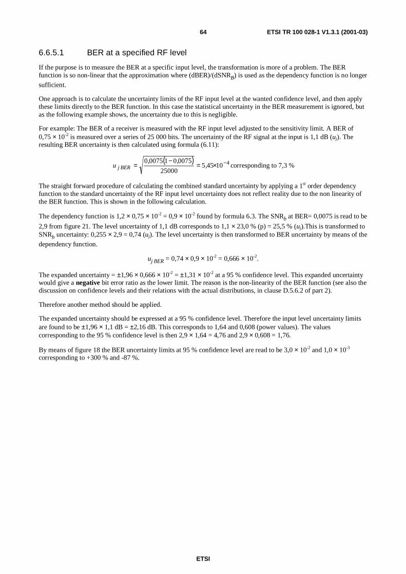
ETSI
ETSI TR 100 028-1 V1.3.1 (2001-03)64
6.6.5.1 BER at a specified RF level
If the purpose is to measure the BER at a specific input level, the transformation is more of a problem. The BERfunction is so non-linear that the approximation where (dBER)/(dSNRB) is used as the dependency function is no longer
sufficient.
One approach is to calculate the uncertainty limits of the RF input level at the wanted confidence level, and then applythese limits directly to the BER function. In this case the statistical uncertainty in the BER measurement is ignored, butas the following example shows, the uncertainty due to this is negligible.
For example: The BER of a receiver is measured with the RF input level adjusted to the sensitivity limit. A BER of0,75 × 10-2 is measured over a series of 25 000 bits. The uncertainty of the RF signal at the input is 1,1 dB (uj). Theresulting BER uncertainty is then calculated using formula (6.11):
( ) 41045525000
00750100750 −×=−
= ,,,
u j BER corresponding to 7,3 %
The straight forward procedure of calculating the combined standard uncertainty by applying a 1st order dependencyfunction to the standard uncertainty of the RF input level uncertainty does not reflect reality due to the non linearity ofthe BER function. This is shown in the following calculation.
The dependency function is 1,2 × 0,75 × 10-2 = 0,9 × 10⁻² found by formula 6.3. The SNRb at BER= 0,0075 is read to be
2,9 from figure 21. The level uncertainty of 1,1 dB corresponds to 1,1 × 23,0 % (p) = 25,5 % (uj).This is transformed toSNRb uncertainty: 0,255 × 2,9 = 0,74 (uj). The level uncertainty is then transformed to BER uncertainty by means of the
dependency function.
uj BER = 0,74 × 0,9 × 10-2 = 0,666 × 10-2.
The expanded uncertainty = ±1,96 × 0,666 × 10-2 = ±1,31 × 10⁻² at a 95 % confidence level. This expanded uncertaintywould give a negative bit error ratio as the lower limit. The reason is the non-linearity of the BER function (see also thediscussion on confidence levels and their relations with the actual distributions, in clause D.5.6.2 of part 2).
Therefore another method should be applied.
The expanded uncertainty should be expressed at a 95 % confidence level. Therefore the input level uncertainty limitsare found to be ±1,96 × 1,1 dB = ±2,16 dB. This corresponds to 1,64 and 0,608 (power values). The valuescorresponding to the 95 % confidence level is then 2,9 × 1,64 = 4,76 and 2,9 × 0,608 = 1,76.
By means of figure 18 the BER uncertainty limits at 95 % confidence level are read to be 3,0 × 10⁻² and 1,0 × 10⁻³
corresponding to +300 % and -87 %.

ETSI
ETSI TR 100 028-1 V1.3.1 (2001-03)65
1 2 3 7 8 9 10 11 12654Signal to noise ratio per bit SNRb (in linear terms)
BE
R(S
NR
b)fo
rco
here
ntm
odul
atio
n
10-4
10-3
10-2
10-1
1,5
2,0
3,0
4,05,06,0
8,0
1,5
2,0
3,0
4,05,06,0
1,5
2,0
3,0
4,05,06,0
1,5
2,0
3,0
4,05,06,0
1,5
2,0
3,0
4,05,06,0
8,0
8,0
8,0
8,0
10-6
10-5
Figure 18: BER (SNRb) against SNRb
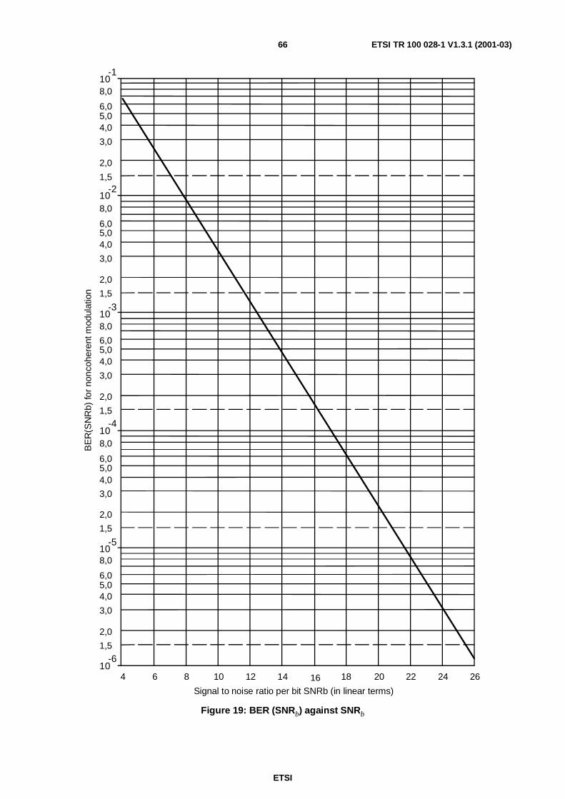
ETSI
ETSI TR 100 028-1 V1.3.1 (2001-03)66
4 6 8 16 18 20 22 24 26141210
Signal to noise ratio per bit SNRb (in linear terms)
BE
R(S
NR
b)fo
rno
ncoh
eren
tmod
ulat
ion
10-6
10-5
10-4
10-3
10-2
10-1
1,5
2,0
3,0
4,05,06,0
8,0
1,5
2,0
3,0
4,05,06,0
1,5
2,0
3,0
4,05,06,0
1,5
2,0
3,0
4,05,06,0
1,5
2,0
3,0
4,05,06,0
8,0
8,0
8,0
8,0
Figure 19: BER (SNRb) against SNRb
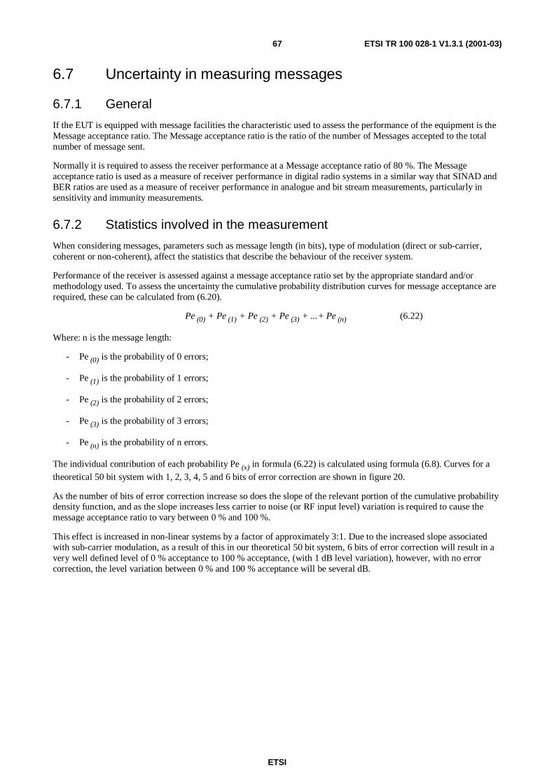
ETSI
ETSI TR 100 028-1 V1.3.1 (2001-03)67
6.7 Uncertainty in measuring messages
6.7.1 General
If the EUT is equipped with message facilities the characteristic used to assess the performance of the equipment is theMessage acceptance ratio. The Message acceptance ratio is the ratio of the number of Messages accepted to the totalnumber of message sent.
Normally it is required to assess the receiver performance at a Message acceptance ratio of 80 %. The Messageacceptance ratio is used as a measure of receiver performance in digital radio systems in a similar way that SINAD andBER ratios are used as a measure of receiver performance in analogue and bit stream measurements, particularly insensitivity and immunity measurements.
6.7.2 Statistics involved in the measurement
When considering messages, parameters such as message length (in bits), type of modulation (direct or sub-carrier,coherent or non-coherent), affect the statistics that describe the behaviour of the receiver system.
Performance of the receiver is assessed against a message acceptance ratio set by the appropriate standard and/ormethodology used. To assess the uncertainty the cumulative probability distribution curves for message acceptance arerequired, these can be calculated from (6.20).
Pe (0) + Pe (1) + Pe (2) + Pe (3) + ...+ Pe (n) (6.22)
Where: n is the message length:
- Pe (0) is the probability of 0 errors;
- Pe (1) is the probability of 1 errors;
- Pe (2) is the probability of 2 errors;
- Pe (3) is the probability of 3 errors;
- Pe (n) is the probability of n errors.
The individual contribution of each probability Pe (x) in formula (6.22) is calculated using formula (6.8). Curves for atheoretical 50 bit system with 1, 2, 3, 4, 5 and 6 bits of error correction are shown in figure 20.
As the number of bits of error correction increase so does the slope of the relevant portion of the cumulative probabilitydensity function, and as the slope increases less carrier to noise (or RF input level) variation is required to cause themessage acceptance ratio to vary between 0 % and 100 %.
This effect is increased in non-linear systems by a factor of approximately 3:1. Due to the increased slope associatedwith sub-carrier modulation, as a result of this in our theoretical 50 bit system, 6 bits of error correction will result in avery well defined level of 0 % acceptance to 100 % acceptance, (with 1 dB level variation), however, with no errorcorrection, the level variation between 0 % and 100 % acceptance will be several dB.

ETSI
ETSI TR 100 028-1 V1.3.1 (2001-03)68
Cumulative probability distribution
level (dB)2 3 4 5 6 7 8
0,0
10
20
30
40
50
60
70
80
90
100
9 10 11 12
Pro
babi
lity(
%)
Figure 20: Cumulative Probability (error correction for Messages)
As a method of testing receivers the "up-down" method is used. The usage of the up down method will result in a seriesof transmissions using a limited number of RF levels.
6.7.3 Analysis of the situation where the up down method results in a shiftbetween two levels
With some systems (e.g. 6 bits of error correction) the up-down method will typically result in a pattern shiftingbetween two levels, where at the lower level the message acceptance ratio will approach zero and at the higher level(+1 dB) the message acceptance ratio will approach 100 %. In this case the measurement uncertainty is of the simplestform for this contribution.
The RF is switching between two levels, the mean value is calculated, usually from 10 or 11 measurements. Themeasurement uncertainty cannot be calculated as though random, independent sources are involved. The RF isswitching between two output levels of the same signal generator, the levels therefore are correlated and only have twovalues (upper and lower), hence the standard uncertainty for a signal generator with output level uncertainty of ±1 dBis:
dB0,583
01 == ,u levelj output
Also there is a quantization uncertainty associated with half of the step size (in this case 1 dB which gives ±0,5 dB).
dB0,293
50 == ,u ationj quantisi
Therefore the combined standard uncertainty of this step will be:
dB0,65290580 2222 =+=+= ,,uuu tionj quantisalevelj outputshiftleveltwoc
For the case of no error correction the pattern of the measured results will spread beyond a single dB step andmeasurement uncertainty calculations are more complex.

ETSI
ETSI TR 100 028-1 V1.3.1 (2001-03)69
6.7.4 Detailed example of uncertainty in measuring messages
For this example a theoretical system with 50 bit message length and 1 bit error correction will be considered, althoughthe principles can be applied to all practicable message and correction lengths.
a) Calculate the message acceptance ratio (formula (6.22)) for the given message length and given number of biterror corrections, using bit error ratios corresponding to a convenient step size (in this case 1 dB) using eitherformula (6.18) for non-coherent, or, formula (6.12) for coherent, and if sub-carrier modulation is used, use theappropriate SINAD conversion in ETR 028 [15], part 2, annex F, table F.1.
b) Now the probability of being at a given point on the curve must be assessed. For example the probability ofbeing at a particular point (in figure 20) is:
- the probability of being below a particular point times the probability of going up from this point; plus
- the probability of being above a particular point times the probability of going down from this point.
The method requires three successful responses, therefore the probability of going up is:
Pp (up) = 1 - (Message Acceptance)3 = 1- (MA)3 (6.23)
and the probability of going down is:
Pp (down) = (Message Acceptance)3 = (MA)3 (6.24)
(Pe (0) + Pe (1)) = Probability of 0 errors + the probability of 1 error (see formula (6.24)). These calculations are shown
in table 2.
Table 2: Probability of going up or down from a given position
dB Linear BER (Pe(0)+Pe(1))% Pp (up)=1- (MA)3 Pp (down)= (MA)3
+2 12,679 0,8826 × 10⁻³ 99,91 2,698 × 10-3 997,3 × 10⁻³
+1 10,071 3,251 × 10-3 98,83 34,69 × 10⁻³ 965,3 × 10⁻³
0 8,000 9,158 × 10-3 92,30 213,7 × 10⁻³ 786,3 × 10⁻³
-1 6,355 20,84 × 10⁻³ 72,02 626,4 × 10⁻³ 373,6 × 10⁻³
-2 5,048 40,07 × 10⁻³ 39,95 936,2 × 10⁻³ 63,76 × 10⁻³
-3 4,010 67,33 × 10⁻³ 14,13 997,2 × 10⁻³ 2,821 × 10-3
-4 3,185 101,7 × 10⁻³ 3,123 1,000 30,46 × 10⁻⁶
-5 2,530 141,1 × 10⁻³ 0,459 1,000 96,55 × 10⁻⁹
Based on equations (6.21) and (6.22), and the fact that the sum of all probabilities equals 1, the individual probabilitiesof being at each step of the signal to noise ratio per bit (SNRb) can be calculated.
Assuming that at SNRb greater than +1 dB all messages are accepted (therefore can only move down from here) and
Assuming that at SNRb less than -4 dB all messages are rejected (therefore can only move up from here), this gives riseto two boundary positions -5 dB and +2 dB.
The probability of being at any one of the points -5, -4, -3, -2, -1, 0, +1, +2 is Pp-5, Pp-4, Pp-3, Pp-2, Pp-1, Pp0, Pp+1, andPp+2 respectively.
The analysis of the possible transitions between these points provide:
- Pp-5 = (Pp-4+ 30,46 × 10⁻⁶) + (Pp-6 × 1);
- Pp-4 = (Pp-3 × 2,821 × 10-3) + (Pp-5 × 1);
- Pp-3 = (Pp-2 × 63,76 × 10-3) + (Pp-4 × 1);
- Pp-2 = (Pp-1 × 373,6 × 10-3) + (Pp-3 × 997,2 × 10-3);

ETSI
ETSI TR 100 028-1 V1.3.1 (2001-03)70
- Pp-1 = (Pp0 × 786,3 × 10-3) + (Pp-2 × 936,2 × 10-3);
- Pp0 = (Pp+1 × 965,3 × 10-3) + (Pp-1 × 626,4 × 10-3);
- Pp+1 = (Pp+2 × 1) + (Pp0 × 213,7 × 10-3);
- Pp+2 = (Pp+3 × 1) + (Pp+1 × 34,69 × 10-3).
NOTE: The probability of being at point Pp-6 or Pp+3 is zero, hence Pp-6 × 1 and Pp+3 × 1 are both equal to zero.
Based on seven out of these eight equations and the fact that the sum of Pp-5 to Pp+2 is one, each individual probabilityPp-5 to Pp+2 is calculated as follows.
Rearranging the above equations gives:
- Pp-6 × 1 - Pp-5 + Pp-4 × 30,46 × 10-6 = 0;
- Pp-5 × 1 - Pp-4+ Pp-3 × 2,821 × 10-3 = 0;
- Pp-4 × 1 - Pp-3+ Pp-2 × 63,76 × 10-3 = 0;
- Pp-3 × 997,3 × 10-3 - Pp-2+ Pp-1 × 373,6 × 10-3 = 0;
- Pp-2 × 936,2 × 10-3 - Pp-1+ Pp0 × 786,3 × 10-3 = 0;
- Pp-1 × 626,4 × 10-3 - Pp0+ Pp+1 × 965,3 × 10-3 = 0;
- Pp0 × 213,7 × 10-3 - Pp+1+ Pp+2 × 1 = 0;
- Pp+1 × 34,69 × 10-3 - Pp+2 + Pp+3 × 1 = 0;
- Pp-5 + Pp-4 +Pp-3 + Pp-2+ Pp-1 + Pp0+ Pp+1+ Pp+2 = 1;
- Pp-6 = Pp+3 = 0.
Pp-5 Pp-4 Pp-3 Pp-2 Pp-1 Pp0 Pp+1 Pp+21 1 -1 2,821 × 10-3
2 1 -1 63,76 × 10⁻³
3 997,3 × 10⁻³ -1 373,6 × 10⁻³
4 936,2 × 10⁻³ -1 786,3 × 10⁻³
5 626,4 × 10⁻³ -1 965,3 × 10⁻³
6 213,7 × 10⁻³ -1 17 34,69 × 10⁻³ -18 1 1 1 1 1 1 1 1 1
Solving this by means of row operations on row 8, gives:
1 1 -1 2,821 ×××× 10-3
2 1 -1 63,76 × 10⁻³
3 997,3 × 10⁻³ -1 373,6 × 10⁻³
4 936,2 × 10⁻³ -1 786,3 × 10⁻³
5 626,4 × 10⁻³ -1 965,3 × 10⁻³
6 213,7 × 10⁻³ -1 17 34,69 × 10⁻³ -18 392,91 1

ETSI
ETSI TR 100 028-1 V1.3.1 (2001-03)71
From this we have: 392,91 × Pp+2 = 1; therefore Pp+2 = 2,545 × 10-3:
- this is then used in row 7 to determine Pp+1: 33
3
1 103673106934
105452 −−
−
+ ×=×
×= ,
,
,Pp ;
- this is used in row 6 to determine Pp0:( ) 3
3
3
0 1038331107213
1105452073360 −−
−×=
×
××−= ,
,
,,Pp ;
- this is used in row 5 to determine Pp-1:( ) 3
3
333
1 1097415104626
1039651036731038331 −−
−−−
− ×=×
×××−×= ,
,
,,,Pp ;
- this is used in row 4 to determine Pp-2:( ) 3
3
2 10016693620
786303313801097415 −−
− ×=×−×
= ,,
,,,Pp ;
- this is used in row 3 to determine Pp-3:( ) 3
3
3 106221099730
373604159701000166 −−
− ×=×−×
= ,,
,,,Pp ;
- this is used in row 2 to determine Pp-4:( ) 6
33
4 1084371
107663166001062210 −−−
− ×=××−×
= ,,,,
Pp ;
- this is used in row 1 to determine Pp-5:( ) 6
336
5 108771
1082121062210108437 −−−−
− ×=×××−×
= ,,,,
Pp .
There are, off course, other ways of solving the equations.
After having calculated the probabilities it should always be checked that the sum of all probabilities is 1. If the sum isnot 1 (to within 0,001) it can cause major uncertainties in the calculation of the resulting standard uncertainty of thedistribution.
Based on these probabilities the standard uncertainty of the distribution is calculated:
∑=
−=
−=×=2
5
700i
i
i ,iPpX (formula 5.6)
∑=
−=
=×=2
5
2 261i
i
i ,iPpY (formula 5.7)
then:
( ) dB0,88700261 22 =−−=−= ,,XYu j (formula 5.8)
and the standard uncertainty for the measurement (as the result is the average value of 10 samples):
dB0,2810
880 =,(formula 5.9)
The expanded uncertainty is ±1,96 × 0,28 = ±0,54 dB at a 95 % confidence level.
Therefore the methodology introduces an additional ±0,54 dB of uncertainty to the level.

ETSI
ETSI TR 100 028-1 V1.3.1 (2001-03)72
6.8 Examples of measurement uncertainty analysis (Free FieldTest Sites)
6.8.1 Introduction
This clause contains detailed worked examples of the calculation of expanded uncertainty of the radiated tests on FreeField Test Sites i.e. Anechoic Chambers, Anechoic Chamber with a ground plane and Open Area Test Sites.
The example tests given are limited to:
- a verification procedure;
- the measurement of a transmitter parameter (spurious emission);
- the measurement of a receiver parameter (sensitivity).
All the example tests are assumed to have been carried out in an Anechoic Chamber with a ground plane since this typeof test site will contribute virtually all the uncertainty contributions involved in radiated tests on any Free Field Test Site(i.e. all uncertainties associated with absorbing materials and ground planes).
NOTE 1: The values given to the uncertainty components in these examples are only to illustrate the uncertaintycalculations. In practice, values should be derived by consulting annex A.
All radiated tests consist of two stages. For a verification procedure, the first stage is to set a reference level whilst thesecond stage involves the measurement of path loss between two antennas. For the measurement of a particularparameter from an EUT, the first stage is usually to measure the relevant parameter whilst the second stage comparesthis measurement against that from a known standard.
Within any radiated test there are uncertainty components that are common to both stages of the test. By their differentnatures some of these common uncertainties will cancel (e.g. the uncertainty of the insertion loss of a cable common toboth parts) whilst others may contribute twice (e.g. the level stability of a signal generator in receiver tests). In each ofthe following uncertainty analyses, uncertainty components common to both stages are shown as shaded areas in theaccompanying schematic diagrams.
As shown in the examples, all the individual uncertainty components for any test are combined in the manner describedin ETR 273 [12], part 1, subpart 1, clauses 4 and 5 in order to derive an expanded uncertainty figure for themeasurement. The values of the individual components are either provided in annex A or should be taken frommanufacturers' data sheets. Whenever they are obtained from data sheets, worst case figures given over a frequencyband should be used. For example, in the case of a signal generator whose absolute level accuracy is quoted as ±1 dBover 30 MHz to 300 MHz, ±2 dB over 300 MHz to 1 000 MHz the figure for the band containing the test frequencyshould be used. This approach should be adopted for all uncertainty components, taking the uncertainty figures over asbroad a band a possible. This is normally satisfactory when the variation with frequency is not large and provides asimple and flexible approach. The resulting expanded uncertainty figure is valid across a broad range of frequencies andmeasurement conditions and avoids the necessity of repeated calculation for minor frequency changes.
NOTE 2: Taking specific frequency values may result in a lower expanded uncertainty value, but this lower value isonly valid when that specific set of circumstances apply for which the value was derived.
6.8.2 Example 1: Verification procedure
The verification procedure is a process carried out to prove a facility's suitability as a Free Field Test Site. It involvesthe transmission of a known signal level from one calibrated antenna (usually a dipole) and the measurement of thereceived signal level in a second calibrated antenna (also usually a dipole). By comparison of the transmitted andreceived signal levels, an "insertion loss" can be deduced.
For the measurement of NSA two stages are involved. The first is a direct attenuation measurement (Vdirect) whilst thesecond is a radiated attenuation measurement (Vsite). After inclusion of any correction factors relevant to themeasurement, the figure of loss which results from the verification procedure is known as "Site Attenuation".
NSA is determined from the value of Site Attenuation by subtraction of the antenna factors and mutual coupling effects.The subtraction of the antenna factors and any mutual coupling effects makes NSA independent of antenna type.
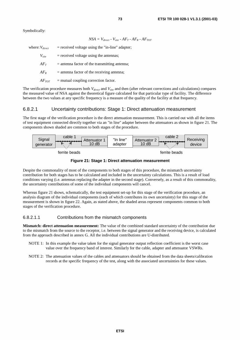
ETSI
ETSI TR 100 028-1 V1.3.1 (2001-03)73
Symbolically:
NSA = Vdirect - Vsite - AFT - AFR - AFTOT
where:Vdirect = received voltage using the "in-line" adapter;
Vsite = received voltage using the antennas;
AFT = antenna factor of the transmitting antenna;
AFR = antenna factor of the receiving antenna;
AFTOT = mutual coupling correction factor.
The verification procedure measures both Vdirect and Vsite and then (after relevant corrections and calculations) comparesthe measured value of NSA against the theoretical figure calculated for that particular type of facility. The differencebetween the two values at any specific frequency is a measure of the quality of the facility at that frequency.
6.8.2.1 Uncertainty contributions: Stage 1: Direct attenuation measurement
The first stage of the verification procedure is the direct attenuation measurement. This is carried out with all the itemsof test equipment connected directly together via an "in line" adapter between the attenuators as shown in figure 21. Thecomponents shown shaded are common to both stages of the procedure.
"In line"adapter
Attenuator 210 dB
Receivingdevice
Attenuator 110 dB
Signalgenerator
cable 1 cable 2
ferrite beads ferrite beads
Figure 21: Stage 1: Direct attenuation measurement
Despite the commonality of most of the components to both stages of this procedure, the mismatch uncertaintycontribution for both stages has to be calculated and included in the uncertainty calculations. This is a result of loadconditions varying (i.e. antennas replacing the adapter in the second stage). Conversely, as a result of this commonality,the uncertainty contributions of some of the individual components will cancel.
Whereas figure 21 shows, schematically, the test equipment set-up for this stage of the verification procedure, ananalysis diagram of the individual components (each of which contributes its own uncertainty) for this stage of themeasurement is shown in figure 22. Again, as stated above, the shaded areas represent components common to bothstages of the verification procedure.
6.8.2.1.1 Contributions from the mismatch components
Mismatch: direct attenuation measurement: The value of the combined standard uncertainty of the contribution dueto the mismatch from the source to the receptor, i.e. between the signal generator and the receiving device, is calculatedfrom the approach described in annex G. All the individual contributions are U-distributed.
NOTE 1: In this example the value taken for the signal generator output reflection coefficient is the worst casevalue over the frequency band of interest. Similarly for the cable, adapter and attenuator VSWRs.
NOTE 2: The attenuation values of the cables and attenuators should be obtained from the data sheets/calibrationrecords at the specific frequency of the test, along with the associated uncertainties for these values.

ETSI
ETSI TR 100 028-1 V1.3.1 (2001-03)74
Receivingdevice
Cableloss
Receivingdevice
Signalgenerator
Cableloss
Cablefactor
Receivingantennacable 2
Transmittingantennacable 1
sourceTransmitting
Adaptor
Mismatch
Attenuator 110 dB
Mismatch
++
+ + Attenuator 210 dB
Cablefactor
Mismatch
MismatchMismatch
Mismatch+
+ +
+
Figure 22: Stage 1: Direct attenuation measurement individual uncertainty components
Signal generator: Output reflection coefficient: |ρG| = 0,20
Cable: Input and output reflection coefficients: |S11| = |S22| = 0,07
Attenuation: 1 dB = |S12| = |S21| = 0,891
Attenuator: Input and output reflection coefficients |S11| = |S22| = 0,05
Attenuation = 10 dB |S12| = |S21| = 0,3162
Adapter: Input and output reflection coefficients |S11| = |S22| = 0,02
Attenuation = 0,1 dB |S12| = |S21| = 0,9886
Attenuator: Input and output reflection coefficients |S11| = |S22| = 0,05
Attenuation = 10 dB |S12| = |S21| = 0,3162
Cable: Input and output reflection coefficients: |S11| = |S22| = 0,07
Attenuation: 1 dB = |S12| = |S21| = 0,891
Receiving device: Input reflection coefficient: |ρRD| = 0,20
Mismatch uncertainty in the direct attenuation measurement: In the following the transmitting antenna cable isnamed cable 1, the transmitting antenna attenuator is named attenuator 1, the receiving antenna cable is named cable 2,the receiving attenuator is named attenuator 2. Those components that are constant for both stages 1 and 2 are notcalculated as they do not contribute to the overall uncertainty.

ETSI
ETSI TR 100 028-1 V1.3.1 (2001-03)75
Mismatch between:
- uj generator and cable 1: Constant for both stage 1 and 2. Hence this value does not contribute.
- uj cable 1 and attenuator 1: Constant for both stage 1 and 2. Hence this value does not contribute.
%0,071%2
10002,005,01: =××=adapterandattenuatormismatchju
%0,071%2
10005,002,01: =××=attenuatorandadaptermismatchju
- uj attenuator 2 and cable 2: Constant for both stage 1 and 2. Hence this value does not contribute.
- uj cable 2 and receiving device: Constant for both stage 1 and 2. Hence this value does not contribute.
- uj generator and attenuator 1: Constant for both stage 1 and 2. Hence this value does not contribute.
%0,035%2
100316,007,007,0 2
1: =×××=adapterandcablemismatchju
%0,173%2
100988,005,005,0 2
21: =×××=attenuatorandattenuatormismatchju
%0,010%2
100316,007,002,0 2
2: =×××=cableandadaptermismatchju
- uj attenuator 2 and receiving device: Constant for both stage 1 and 2. Hence this value does not contribute.
%0,022%2
100316,0891,002,02,0 22
: =××××=adapterandgeneratormismatchju
%0,024%2
100988,0316,005,007,0 22
21: =××××=attenuatorandcablemismatchju
%0,024%2
100316,0988,007,005,0 22
21: =××××=cableandattenuatormismatchju
%0,022%2
100891,0316,02,002,0 22
: =××××=devicereceivingandadaptermismatchju
%0,055%2
100988,0316,0891,005,02,0 222
2: =×××××=attenuatorandgeneratormismatchju
- uj mismatch: cable 1 and cable 2: Less than 0,01 % due to the two attenuators, therefore neglected.
%0,055%2
100891,0316,0988,02,005,0 222
1: =×××××=devicereceivingandattenuatormismatchju
- uj mismatch: generator and cable 2: Less than 0,01 % due to the two attenuators, therefore neglected.
- uj mismatch: cable 1 and receiving device: Less than 0,01 % due to the two attenuators, therefore neglected.
- uj mismatch: generator and receiving device: Less than 0,01 % due to the two attenuators, therefore neglected.

ETSI
ETSI TR 100 028-1 V1.3.1 (2001-03)76
The combined standard uncertainty of the mismatch is then calculated:
%0,306055,0055,0...071,0071,0 2222.: =++++=attdirectmismatchcu
Transforming to logarithmic form (ETR 028 [15], part 2, annex E): 0,306 %/11,5 = 0,026 dB.
The standard uncertainty of the contribution, due to the mismatch in the direct attenuation measurement, is designatedthroughout all parts of ETR 273 [12] as uj35. Its value in this example is 0,026 dB.
6.8.2.1.2 Contributions from individual components
6.8.2.1.2.1 Signal generator
Signal generator: absolute output level: In a verification procedure, the signal generator's absolute level uncertaintycontributes equally to both stages of the measurement. The standard uncertainty of the contribution due to the signalgenerator absolute output level uncertainty is designated throughout all parts of ETR 273 [12] as uj38.
NOTE 1: In this example case the standard uncertainty of the contribution due to the signal generator absoluteoutput level uncertainty is taken to be 0,00 dB since, once the level has been set in stage one of theprocedure, the level is not further adjusted. The uncertainty is therefore assumed to be systematic i.e. itproduces the same offset in both stages.
Signal generator: output level stability: In any test in which the contribution of the absolute level uncertainty of thesignal generator contributes to the combined standard uncertainty of the test i.e. it does not cancel due to themethodology, the contribution from the output level stability is considered to have been included in the signal generatorabsolute output level, uj38. Conversely, for any level in which the absolute level uncertainty of the signal generator doesnot contribute to the combined standard uncertainty, the output level stability of the signal generator should be included.The standard uncertainty of the contribution due to the signal generator output level stability is designated throughoutall parts of ETR 273 [12] as uj39. Its value can be derived from manufacturers' data sheet.
NOTE 2: In this example case the uncertainty of the contribution due to the signal generator output level stability isobtained from the manufacturers data sheet as ±0,02 dB. As nothing is said about the distribution of thisuncertainty, a rectangular distribution (see ETR 273 [12], part 1, subpart 1, clause 5.1.2) in logs isassumed, and the standard uncertainty is calculated as 0,01155 dB. This is rounded down to 0,01 dB.
6.8.2.1.2.2 Transmitting antenna cable
Insertion loss: transmitting antenna cable: The transmitting antenna cable has an insertion loss as well as anuncertainty associated with the measurement of its magnitude. The value of insertion loss and its uncertainty remainvalid provided the cable is not used outside the manufacturer's specification. At any given frequency the insertion lossacts as a systematic offset and contributes equally to both stages of the measurement. The standard uncertainty of thecontribution due to the insertion loss uncertainty of the transmitting antenna cable is designated throughout all parts ofETR 273 [12] as uj41.
NOTE 1: In this example case the standard uncertainty of the contribution due to the insertion loss uncertainty ofthe transmitting antenna cable is taken as 0,00 dB since the uncertainty is systematic i.e. it produces thesame offset in both stages.
Cable factor: transmitting antenna: Cable factor is defined as the total effect of the antenna cable's influence on themeasuring system including its interaction with the site. It consists of the leakage caused by cable screeninginefficiency, parasitic effects on the transmitting antenna (acting as a director or reflector) and introducing anunbalanced, common mode current into the dipole balun. In a radiated measurement the standard uncertainty of thecable factor, associated with each cable, is 0,5 dB provided that the precautions detailed in the methods have beenobserved i.e. routing and dressing of cables with ferrites. If no prevention has been attempted the standard uncertainty is4,0 dB (justification for these values is given in ETR 273 [12], part 1, subpart 2, annex E). The standard uncertainty ofthe contribution due to the cable factor of the transmitting antenna cable is designated throughout all parts ofETR 273 [12] as uj19.
NOTE 2: In this example case the standard uncertainty of the contribution due to the cable factor of the transmittingantenna cable is taken as 0,00 dB since there are no external fields involved other than leakage, which isassumed to have a negligible effect on the measurement.

ETSI
ETSI TR 100 028-1 V1.3.1 (2001-03)77
6.8.2.1.2.3 Transmitting antenna attenuator
Insertion loss: transmitting antenna attenuator: The transmitting antenna attenuator has an insertion loss as well asan uncertainty associated with the measurement of its magnitude. The value of insertion loss and its uncertainty remainvalid provided the attenuator is not used outside the manufacturer's specification. At any given frequency the insertionloss acts as a systematic offset and contributes equally to both stages of the measurement. The standard uncertainty ofthe contribution, due to the insertion loss uncertainty of the transmitting antenna attenuator, is designated throughout allparts of ETR 273 [12] as uj40.
NOTE: In this example case the standard uncertainty of the contribution due to the insertion loss uncertainty ofthe transmitting antenna attenuator is taken as 0,00 dB since the uncertainty is systematic i.e. it producesthe same offset in both stages.
6.8.2.1.2.4 Adapter
Insertion loss: adapter: The adapter has an insertion loss as well as an uncertainty associated with the measurement ofits magnitude. The value of insertion loss and its uncertainty remain valid provided the adapter is not used outside themanufacturer's specification. The standard uncertainty of the contribution due to the insertion loss uncertainty of theadapter is designated throughout all parts of ETR 273 [12] as uj42. Its value can be derived from the manufacturer's datasheet.
NOTE: In this example case the uncertainty of the contribution due to the insertion loss uncertainty of the adapteris obtained from the manufacturer's data sheet as ±0,10 dB. As nothing is said about the distribution ofthis uncertainty, a rectangular distribution (see ETR 273 [12], part 1, subpart 1, clause 5.1.2) in logs isassumed, and the standard uncertainty is calculated as 0,06 dB.
6.8.2.1.2.5 Receiving antenna attenuator
Insertion loss: receiving antenna attenuator: The attenuator has an insertion loss as well as an uncertainty associatedwith the measurement of its magnitude. The value of insertion loss and its uncertainty remain valid provided theattenuator is not used outside the manufacturer's specification. At any given frequency the insertion loss acts as asystematic offset and contributes equally to both stages of the measurement. The standard uncertainty of thecontribution due to the insertion loss uncertainty of the receiving antenna attenuator is designated throughout all parts ofETR 273 [12] as uj40.
NOTE: In this example case the standard uncertainty of the contribution due to the insertion loss uncertainty ofthe receiving antenna attenuator is taken as 0,00 dB since the uncertainty is systematic i.e. it produces thesame offset in both stages.
6.8.2.1.2.6 Receiving antenna cable
Insertion loss: receiving antenna cable: The receiving antenna cable has an insertion loss as well as an uncertaintyassociated with the measurement of its magnitude. The value of insertion loss and its uncertainty remain valid providedthe cable is not used outside the manufacturer's specification. At any given frequency the insertion loss acts as asystematic offset and contributes equally to both stages of the measurement. The standard uncertainty of thecontribution, due to the insertion loss uncertainty of the receiving antenna cable, is designated throughout all parts ofETR 273 [12] as uj41.
NOTE 1: In this example case the standard uncertainty of the contribution due to the insertion loss uncertainty ofthe receiving antenna cable is taken as 0,00 dB since the uncertainty is systematic i.e. it produces thesame offset in both stages.
Cable factor: receiving antenna cable: Cable factor is defined as the total effect of the antenna cable's influence onthe measuring system including its interaction with the site. It consists of the leakage caused by cable screeninginefficiency, parasitic effects on the receiving antenna (acting as a director or reflector) and introducing an unbalanced,common mode current into the dipole balun. In a radiated measurement the standard uncertainty of the cable factor,associated with each cable is 0,5 dB provided that the precautions detailed in the methods have been observed.i.e. routing and dressing of cables with ferrites. If no prevention has been attempted the standard uncertainty is 4,0 dB(justification for these values is given in ETR 273 [12], part 1, subpart 2, annex E). The standard uncertainty of thecontribution due to the cable factor of receiving antenna cable is designated throughout all parts of ETR 273 [12] asuj19.

ETSI
ETSI TR 100 028-1 V1.3.1 (2001-03)78
NOTE 2: In this example case the standard uncertainty of the contribution due to the cable factor of the receivingantenna cable is taken as 0,00 dB since there are no external fields involved other than leakage, which isassumed to have a negligible effect on the measurement.
6.8.2.1.2.7 Receiving device
In this, the first stage of the verification procedure, a reference level is recorded from the receiving device for aparticular output level from the signal generator. In the second stage (where the path loss between the two antennas ismeasured), a second level is recorded on the receiving device. Only in the second stage do the linearity and absolutelevel uncertainties of the receiver become involved in the calculation of the combined standard uncertainty of themeasurement.
Receiving device: absolute level: The standard uncertainty of the contribution due to the absolute level uncertainty ofthe receiving device is designated throughout all parts of ETR 273 [12] as uj47.
NOTE 1: In this example case the standard uncertainty of the contribution due to the absolute level uncertainty ofthe receiving device is assumed to be 0,00 dB since, in this part of the measurement, a reference level isrecorded.
Receiving device: linearity: The standard uncertainty of the contribution due to the receiving device linearity isdesignated throughout all parts of ETR 273 [12] as uj48.
NOTE 2: In this example case the standard uncertainty of the contribution due to the receiving device linearity isassumed to be 0,00 dB since, in this part of the measurement, a reference level is recorded.
6.8.2.1.3 Contribution from the random component
Random uncertainty: The magnitude can be assessed from multiple measurements of the direct attenuationmeasurement. The standard uncertainty of the contribution due to the random uncertainty is designated throughout allparts of ETR 273 [12] as ui01. Its value can then be calculated.
The direct attenuation measurement was repeated 10 times. The following results were obtained in dBµV (beforecorrecting for cabling and attenuator network insertion loss):
- 106,8; 107,2; 106,7; 107,0; 107,2; 106,7; 107,1; 106,8; 107,1; 107,0.
Converting to linear terms:
- 0,2188; 0,2291; 0,2163; 0,2239; 0,2291; 0,2163; 0,2265; 0,2188; 0,2265; 0,2239.
The two sums X and Y are calculated:
- X = the sum of the measured values = 2,2292 V;
- Y = the sum of the squares of the measured values = 0,4972 V2.
=−
−=
−
−=
11010
2292,24972,0
1
22
nn
XY
uc random 5,444 ×10-3 (formula 5.6)
As the result is obtained as the mean value of 10 measurements and the standard uncertainty of the random uncertaintyis:
dB0,2125,11
100
22292,0
10444,5 3=××=
−
j randomu
NOTE: In this example case the standard uncertainty of the contribution due to the random uncertainty is0,212 dB.
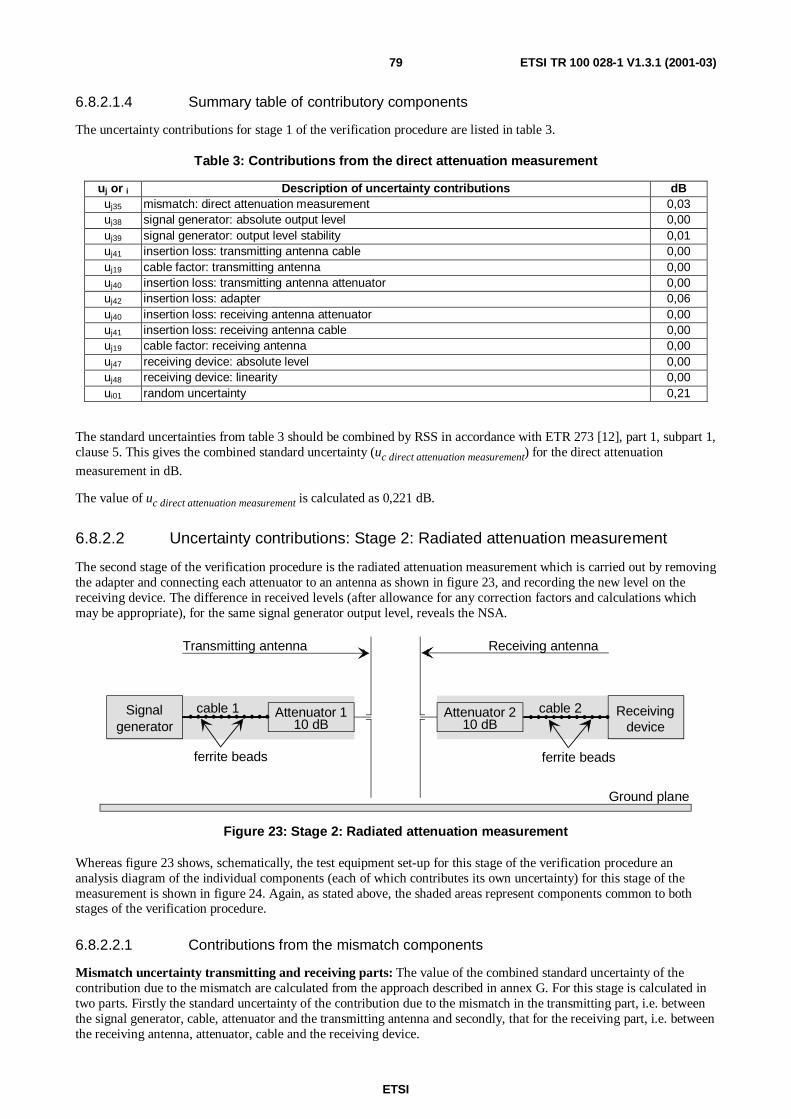
ETSI
ETSI TR 100 028-1 V1.3.1 (2001-03)79
6.8.2.1.4 Summary table of contributory components
The uncertainty contributions for stage 1 of the verification procedure are listed in table 3.
Table 3: Contributions from the direct attenuation measurement
uj or i Description of uncertainty contributions dBuj35 mismatch: direct attenuation measurement 0,03uj38 signal generator: absolute output level 0,00uj39 signal generator: output level stability 0,01uj41 insertion loss: transmitting antenna cable 0,00uj19 cable factor: transmitting antenna 0,00uj40 insertion loss: transmitting antenna attenuator 0,00uj42 insertion loss: adapter 0,06uj40 insertion loss: receiving antenna attenuator 0,00uj41 insertion loss: receiving antenna cable 0,00uj19 cable factor: receiving antenna 0,00uj47 receiving device: absolute level 0,00uj48 receiving device: linearity 0,00ui01 random uncertainty 0,21
The standard uncertainties from table 3 should be combined by RSS in accordance with ETR 273 [12], part 1, subpart 1,clause 5. This gives the combined standard uncertainty (uc direct attenuation measurement) for the direct attenuation
measurement in dB.
The value of uc direct attenuation measurement is calculated as 0,221 dB.
6.8.2.2 Uncertainty contributions: Stage 2: Radiated attenuation measurement
The second stage of the verification procedure is the radiated attenuation measurement which is carried out by removingthe adapter and connecting each attenuator to an antenna as shown in figure 23, and recording the new level on thereceiving device. The difference in received levels (after allowance for any correction factors and calculations whichmay be appropriate), for the same signal generator output level, reveals the NSA.
cable 1
ferrite beads
Attenuator 110 dB
Signalgenerator
cable 2
ferrite beads
Receivingdevice
Attenuator 210 dB
Receiving antennaTransmitting antenna
Ground plane
Figure 23: Stage 2: Radiated attenuation measurement
Whereas figure 23 shows, schematically, the test equipment set-up for this stage of the verification procedure ananalysis diagram of the individual components (each of which contributes its own uncertainty) for this stage of themeasurement is shown in figure 24. Again, as stated above, the shaded areas represent components common to bothstages of the verification procedure.
6.8.2.2.1 Contributions from the mismatch components
Mismatch uncertainty transmitting and receiving parts: The value of the combined standard uncertainty of thecontribution due to the mismatch are calculated from the approach described in annex G. For this stage is calculated intwo parts. Firstly the standard uncertainty of the contribution due to the mismatch in the transmitting part, i.e. betweenthe signal generator, cable, attenuator and the transmitting antenna and secondly, that for the receiving part, i.e. betweenthe receiving antenna, attenuator, cable and the receiving device.

ETSI
ETSI TR 100 028-1 V1.3.1 (2001-03)80
Transmitting antenna
Cablefactor
Receiving antenna
Cablefactor
Antenna to antenna coupling
Mutual image coupling
Antenna factor
+
Cable loss
Receiving deviceSignal generator
Cable loss
+
Antenna factor
Mutual image coupling
Antenna to antenna coupling
Directpath lossReflectedpath loss
SiteImperfections
Receivingantennacable 2
Transmittingantennacable 1
Transmitting Receivingdevicesource
Mismatch
Mismatch Mismatch
Mismatch
MismatchMismatch
+
+
+
+
+
+
Attenuator 2 (10 dB)Attenuator 2 (10 dB)
Figure 24: Stage 2: Radiated attenuation measurement individual uncertainty components
Mismatch: transmitting part:
Signal generator: Output reflection coefficient: |ρG| = 0,20
Cable: Input and output reflection coefficients: |S11| and |S22| = 0,07
Attenuation: 1 dB = |S12| = |S21| = 0,891
Attenuator: Input and output reflection coefficients |S11| = |S22| = 0,05
Attenuation = 10 dB |S12| = |S21| = 0,3162
Transmitting antenna: Input reflection coefficient: |ρTA| = 0,333

ETSI
ETSI TR 100 028-1 V1.3.1 (2001-03)81
All these contributions are U-distributed. Those components that cancel are not calculated. Other contributions are (seeannex G):
- uj mismatch: generator and cable 1: Constant for both stage 1 and 2. Hence this value does not contribute.
- uj mismatch: cable 1 and attenuator 1: Constant for both stage 1 and 2. Hence this value does not contribute.
%,1771%2
100333,005,01: =××=antennaandattenuatormismatchju
- uj generator and attenuator 1: Constant for both stage 1 and 2. Hence this value does not contribute.
%0,165%2
100316,0333,007,0 2
1: =×××=antennaandcablemismatchju
%0,373%2
100316,0891,0333,02,0 22
: =××××=antennaandgeneratormismatchju
The combined standard uncertainty of the mismatch is then calculated:
%251373,0165,0177,1 222: ,u partngtransmittimismatchc =++=
transforming to the logarithmic form (ETR 028 [15], part 2, annex E): 1,25 %/11,5 = 0,11 dB.
The standard uncertainty of the contribution due to the mismatch in the transmitting part, is designated throughout allparts of ETR 273 [12] as uj36. Its value in this example is 0,11 dB.
Mismatch: receiving part:
Receiving antenna: Input reflection coefficient: |ρRA| = 0,333
Attenuator: Input and output reflection coefficients |S11| = |S22| = 0,05
Attenuation = 10 dB |S12| = |S21| = 0,3162
Cable: Input and output reflection coefficients: |S11| and |S22| = 0,07
Attenuation: 1 dB = |S12| = |S21| = 0,891
Receiving device: Input reflection coefficient: |ρRD| = 0,20
%,1771%2
10005,0333,02: =××=attenuatorandantennamismatchju
- uj attenuator 2 and cable 2: Constant for both stage 1 and 2. Hence this value does not contribute.
- uj cable 2 and receiving device: Constant for both stage 1 and 2. Hence this value does not contribute.
%0,165%2
100316,007,0333,0 2
2: =×××=cableandantennamismatchju
- uj attenuator 2 and receiving device: Constant for both stage 1 and 2. Hence this value does not contribute.
%0,373%2
100891,0316,02,0333,0 22
: =××××=devicereceivingandantennamismatchju

ETSI
ETSI TR 100 028-1 V1.3.1 (2001-03)82
The combined standard uncertainty of the mismatch is then calculated:
%251373,0165,0177,1 222: ,u partreceivingmismatchc =++=
Transforming to the logarithmic form (ETR 028 [15], part 2, annex E): 1,25 %/11,5 = 0,11 dB.
The standard uncertainty of the contribution due to the mismatch in the receiving part is designated throughout all partsof ETR 273 [12] as uj37. Its value in this example is 0,11 dB.
6.8.2.2.2 Contributions from individual components
6.8.2.2.2.1 Signal generator
Signal generator: absolute output level: In a verification procedure, the signal generator's absolute level uncertaintycontributes equally to both stages of the measurement. The standard uncertainty of the contribution due to the signalgenerator absolute output level uncertainty is designated throughout all parts of ETR 273 [12] as uj38.
NOTE 1: In this example case the standard uncertainty of the contribution due to the signal generator absoluteoutput level uncertainty is taken to be 0,00 dB since, once the level has been set in stage one of theprocedure, the level is not further adjusted. The uncertainty is therefore assumed to be systematic i.e. itproduces the same offset in both stages.
Signal generator: output level stability: In any test in which the contribution of the absolute level uncertainty of thesignal generator contributes to the combined standard uncertainty of the test i.e. it does not cancel due to themethodology, the contribution from the output level stability is considered to have been included in the signal generatorabsolute output level, uj38. Conversely, for any level in which the absolute level uncertainty of the signal generator doesnot contribute to the combined standard uncertainty, the output level stability of the signal generator should be included.The standard uncertainty of the contribution due to the signal generator output level stability is designated throughoutall parts of ETR 273 [12] as uj39. Its value can be derived from manufacturers' data sheet.
NOTE 2: In this example case the uncertainty of the contribution due to the signal generator output level stability isobtained from the manufacturers data sheet as ±0,02 dB. As nothing is said about the distribution of thisuncertainty, a rectangular distribution (see ETR 273 [12], part 1, subpart 1, clause 5.1.2) in logs isassumed, and the standard uncertainty is calculated as 0,01155 dB. This is rounded down to 0,01 dB.
6.8.2.2.2.2 Transmitting antenna cable
Insertion loss: transmitting antenna cable: The transmitting antenna cable has an insertion loss as well as anuncertainty associated with the measurement of its magnitude. The value of insertion loss and its uncertainty remainvalid provided the cable is not used outside the manufacturer's specification. At any given frequency the insertion lossacts as a systematic offset and contributes equally to both stages of the measurement. The standard uncertainty of thecontribution, due to the insertion loss uncertainty of the transmitting antenna cable, is designated throughout all parts ofETR 273 [12] as uj41.
NOTE 1: In this example case the standard uncertainty of the contribution due to the insertion loss uncertainty ofthe transmitting antenna cable is taken as 0,00 dB since the uncertainty is systematic i.e. it produces thesame offset in both stages.
Cable factor: transmitting antenna cable: Cable factor is defined as the total effect of the antenna cable's influenceon the measuring system including its interaction with the site. It consists of the leakage caused by cable screeninginefficiency, parasitic effects on the transmitting antenna (acting as a director or reflector) and introducing anunbalanced, common mode current into the dipole balun. In a radiated measurement the standard uncertainty of thecable factor, associated with each cable, is 0,5 dB provided that the precautions detailed in the methods have beenobserved. i.e. routing and dressing of cables with ferrites. If no prevention has been attempted the standard uncertaintyis 4,0 dB (justification for these values is given in ETR 273 [12], part 1, subpart 2, annex E). The standard uncertaintyof the contribution due to the cable factor of the receiving antenna cable is designated throughout all parts ofETR 273 [12] as uj19.
NOTE 2: In this example case the standard uncertainty of the contribution due to the cable factor of the transmittingantenna cable is taken as 0,50 dB since the precautions detailed in the methods are assumed to have beenobserved.

ETSI
ETSI TR 100 028-1 V1.3.1 (2001-03)83
6.8.2.2.2.3 Transmitting antenna attenuator
Insertion loss: transmitting antenna attenuator: The transmitting antenna attenuator has an insertion loss as well asan uncertainty associated with the measurement of its magnitude. The value of insertion loss and its uncertainty remainvalid provided the attenuator is not used outside the manufacturer's specification. At any given frequency the insertionloss acts as a systematic offset and contributes equally to both stages of the measurement. The standard uncertainty ofthe contribution, due to the insertion loss uncertainty of the transmitting antenna attenuator, is designated throughout allparts of ETR 273 [12] as uj40.
NOTE: In this example case the standard uncertainty of the contribution due to the insertion loss uncertainty ofthe transmitting antenna attenuator is taken as 0,00 dB since the uncertainty is systematic i.e. it producesthe same offset in both stages.
6.8.2.2.2.4 Transmitting antenna
Antenna: antenna factor of the transmitting antenna: Uncertainty is introduced as a result of the inaccurateknowledge of the antenna factor of the transmitting antenna. The antenna factor contributes only to the radiated part ofthis procedure. The standard uncertainty of the contribution due to the antenna factor uncertainty of the transmittingantenna is designated throughout all parts of ETR 273 [12] as uj44. For ANSI dipoles the value should be obtained fromtable 4.
Table 4: Uncertainty contribution of the antenna factor of the transmitting antenna
Frequency Standard uncertainty of thecontribution
30 MHz ≤ frequency < 80 MHz 1,73 dB80 MHz ≤ frequency < 180 MHz 0,60 dBfrequency ≥ 180 MHz 0,30 dB
NOTE 1: For other antenna types the values should be taken from manufacturers' data sheets. If a value is not giventhe standard uncertainty is 1,0 dB.
NOTE 2: In this example case the standard uncertainty of the contribution due to the antenna factor uncertainty ofthe transmitting antenna is 0,30 dB since ANSI dipoles have been used and the frequency is above180 MHz.
Antenna: tuning of the transmitting antenna: Uncertainty is introduced as a result of the inaccurate tuning of thetransmitting antenna. This only occurs in stage two of the measurement and therefore only contributes to this stage. Thestandard uncertainty of the contribution, due to the tuning uncertainty of the transmitting antenna, is designatedthroughout all parts of ETR 273 [12] as uj46.
NOTE 3: In this example case the standard uncertainty of the contribution due to the tuning uncertainty of thetransmitting antenna is taken as 0,06 dB (see annex A).
Position of the phase centre: transmitting antenna: Uncertainty is introduced as a result of the inaccurate positioningof the phase centre of the transmitting antenna. This only occurs in stage two of the measurement. The standarduncertainty of the contribution, due to the uncertainty in the position of the phase centre of the transmitting antenna, isdesignated throughout all parts of ETR 273 [12] as uj22.
NOTE 4: In this example case the standard uncertainty of the contribution due to the uncertainty in the position ofthe phase centre of the transmitting antenna has been calculated from (±(the offset from axis of rotation)/(range length) x100 %). The positioning uncertainty is ±0,01 m and therefore the worst case uncertainty= 0,01/3,0 = 0,333 %. As the offset can be anywhere between these limits, the uncertainty is taken to berectangularly distributed (see ETR 273 [12], part 1, subpart 1, clause 5.1.2) and the standard uncertainty iscalculated as 0,192 %. This is transformed to the logarithmic form (ETR 028 [15], part 2, annex E), to be0,02 dB.

ETSI
ETSI TR 100 028-1 V1.3.1 (2001-03)84
6.8.2.2.2.5 Site factors
Ambient effect: Uncertainty is introduced as a result of local ambient signals raising the noise floor at the measurementfrequency. The standard uncertainty of the contribution due to the ambient effect is designated throughout all parts ofETR 273 [12] as uj34. The values of the standard uncertainty should be taken from table 5.
Table 5: Uncertainty contribution: Ambient effect
Receiving device noise floor(generator OFF) is within:
Standard uncertainty ofthe contribution
3 dB of measurement 1,57 dB3 dB to 6 dB of measurement 0,80 dB6 dB to 10 dB of measurement 0,30 dB10 dB to 20 dB of measurement 0,10 dB20 dB or more of the measurement 0,00 dB
NOTE 1: In this example case the standard uncertainty of the contribution due to the ambient effect is taken as0,00 dB, since the chamber is assumed to be shielded.
Mutual coupling: transmitting antenna to its images in the absorbing material: This uncertainty is the effect of thechange produced in the antenna's input impedance and/or gain. The standard uncertainty of the contribution due to themutual coupling of the transmitting antenna to its images in the absorbing materials is designated throughout all parts ofETR 273 [12] as uj07.
NOTE 2: In this example case the standard uncertainty of the contribution due to the mutual coupling of thetransmitting antenna to its images in the absorbing materials is taken as 0,5 dB (see annex A).
Mutual coupling: transmitting antenna to its image in the ground plane: This uncertainty is the effect of the changeproduced in the antenna's input impedance and/or gain. The standard uncertainty of the contribution due to the mutualcoupling of the transmitting antenna to its image in the ground plane, designated throughout all parts of ETR 273 [12]as uj15, has a value of 0,00 dB for ANSI dipoles since it is included, where significant, in the mutual coupling andmismatch loss correction factors (see table A.20). For other dipoles the value can be obtained from table 6.
Table 6: Uncertainty contribution of the mutual coupling betweenthe transmitting antenna to its image in the ground plane
Spacing between the antennaand the ground plane
Standard uncertaintyof the contribution
For a vertically polarized antennaspacing ≤ 1,25 λ 0,15 dBspacing > 1,25 λ 0,06 dB
For a horizontally polarized antennaspacing < λ/2 1,15 dB
λ/2 ≤ spacing < 3λ/2 0,58 dB3λ/2 ≤ spacing < 3λ 0,29 dB
spacing ≥ 3λ 0,15 dB
NOTE 3: In this example case the standard uncertainty of the contribution due to mutual coupling between thetransmitting antenna and its image in the ground plane is taken as 0,00 dB as we are assuming the use ofANSI dipoles.
Mutual coupling: transmitting antenna to receiving antenna: This is the effect produced by any change in the gainsof the antennas which results from their close spacing. The standard uncertainty of the contribution due to the mutualcoupling of the transmitting antenna to receiving antenna, is designated throughout all parts of ETR 273 [12] as uj10. Ithas a standard uncertainty of 0,00 dB for ANSI dipoles since it is included, where significant, in the mutual couplingand mismatch loss correction factors. For non-ANSI dipoles the standard uncertainty can be taken from table 7.

ETSI
ETSI TR 100 028-1 V1.3.1 (2001-03)85
Table 7: Uncertainty contribution of the mutual coupling betweenthe transmitting and receiving antenna
Frequency Standard uncertaintyof the contribution
(3 m range)
Standard uncertaintyof the contribution
(10 m range)30 MHz ≤ frequency < 80 MHz 1,73 dB 0,60 dB80 MHz ≤ frequency < 180 MHz 0,6 dB 0,00 dBfrequency ≥ 180 MHz 0,00 dB 0,00 dB
NOTE 4: In this example case the standard uncertainty of the contribution due to mutual coupling between thetransmitting and receiving antennas is taken as 0,00 dB as we are using ANSI dipoles.
Mutual coupling: interpolation of mutual coupling and mismatch loss correction factors, only for ANSI dipoles:The standard uncertainty of the contribution, due to the interpolation of mutual coupling and mismatch loss correctionfactors, is designated throughout all parts of ETR 273 [12] as uj12. It has, for spot frequencies given in table A.20, avalue of 0,00 dB. However, for all other frequencies, the standard uncertainty should be obtained from table 8.
Table 8: Uncertainty contribution of the interpolation of mutual couplingand mismatch loss correction factors
Frequency (MHz) Standard uncertainty ofthe contribution
for a spot frequency given in the table 0,00 dB30 MHz ≤ frequency < 80 MHz 0,58 dB80 MHz ≤ frequency < 180 MHz 0,17 dBfrequency ≥ 180 MHz 0,00 dB
NOTE 5: In this example case the standard uncertainty of the contribution, due to the interpolation of mutualcoupling and mismatch loss correction factors, is taken as 0,00 dB as the frequency is above 180 MHz.
Range length: This contribution is associated with the curvature of the phase front from the transmitting antenna to thereceiving antenna. The standard uncertainty of the contribution, due to range length, is designated throughout all partsof ETR 273 [12] as uj16. The standard uncertainty is 0,00 dB if ANSI dipoles are used. For other types of antenna thestandard uncertainty of the contribution should be obtained from table 9.
Table 9: Uncertainty contribution of the range length (verification)
Range length (i.e. the horizontal distancebetween phase centres)
Standard uncertainty of thecontribution
(d1+d2)2/4λ ≤ range length < (d1+d2)
2/2λ 1,26 dB(d1+d2)
2/2λ ≤ range length < (d1+d2)2/λ 0,30 dB
(d1+d2)2/λ ≤ range length < 2(d1+d2)
2/λ 0,10 dBrange length ≥ 2(d1+d2)
2/λ 0,00 dB
NOTE 6: In table 9, d1 and d2 are the maximum dimensions of the antennas.
NOTE 7: In this example case the standard uncertainty of the contribution, due to the range length, is taken as0,00 dB as we are using ANSI dipoles.
Reflectivity of absorbing material: transmitting antenna to the receiving antenna: This uncertainty is associatedwith the magnitude of the reflections occurring from the side walls, end walls and ceiling. These magnitudes are afunction of the quality of the absorber at the frequency of test. The standard uncertainty of the contribution, due toreflectivity of the absorber material between the transmitting antenna and the receiving antenna, is designatedthroughout all parts of ETR 273 [12] as uj03. The relevant value for this contribution should be taken from table 10.

ETSI
ETSI TR 100 028-1 V1.3.1 (2001-03)86
Table 10: Uncertainty contribution of the reflectivity of absorbing materialbetween the transmitting and receiving antennas
Reflectivity of the absorbing material Standard uncertainty of the contributionreflectivity < 10 dB 4,76 dB10 dB ≤ reflectivity < 15 dB 3,92 dB15 dB ≤ reflectivity < 20 dB 2,56 dB20 dB ≤ reflectivity < 30 dB 1,24 dBreflectivity ≥ 30 dB 0,74 dB
NOTE 8: In this example case the standard uncertainty of the contribution, due to the reflectivity of absorbermaterial between the transmitting antenna and the receiving antenna, is taken as 2,56 dB since it isassumed that the absorber has a reflectivity in the range 15 dB to 20 dB.
Mutual coupling: receiving antenna to its images in the absorbing material: This uncertainty is the effect of thechange produced in the antenna's input impedance and/or gain. The standard uncertainty of the contribution, due to themutual coupling of the receiving antenna to its images in the absorbing material, is designated throughout all parts ofETR 273 [12] as uj07.
NOTE 9: In this example case the standard uncertainty of the contribution due to the mutual coupling of thereceiving antenna to its images in the absorbing material is taken as 0,5 dB.
Mutual coupling: receiving antenna to its image in the ground plane: This uncertainty is the effect of the changeproduced in the antenna's input impedance and/or gain. The standard uncertainty of the contribution, due to the mutualcoupling of the receiving antenna to its image in the ground plane, is designated throughout all parts of ETR 273 [12] asuj15. It has a value of 0,00 dB for ANSI dipoles since it is included, where significant, in the mutual coupling andmismatch loss correction factors. For other antennas the value can be obtained from table 11.
Table 11: Uncertainty contribution of the mutual coupling betweenthe receiving antenna and its image in the ground plane
Spacing between the antennaand the ground plane
Standard uncertaintyof the contribution
For a vertically polarized antennaspacing ≤ 1,25 λ 0,15 dBspacing > 1,25 λ 0,06 dB
For a horizontally polarized antennaspacing < λ/2 1,15 dB
λ/2 ≤ spacing < 3λ/2 0,58 dB3λ/2 ≤ spacing < 3λ 0,29 dB
spacing ≥ 3λ 0,15 dB
NOTE 10:In this example case the standard uncertainty of the contribution due to the mutual coupling between thereceiving dipole and its image in the ground plane is taken as 0,00 dB as we are using ANSI dipoles.
6.8.2.2.2.6 Receiving antenna
Correction: measurement distance: For verification procedures only one stage involves a radiated measurement andhence no correction can be applied i.e. the uncertainty contribution is 0,00 dB. The standard uncertainty of thecontribution, due to the correction for measurement distance, is designated throughout all parts of ETR 273 [12] as uj18.
Correction: off boresight angle in elevation plane: For verification procedures only one stage involves a radiatedmeasurement and hence no correction can be applied i.e. the uncertainty contribution is 0,00 dB. The standarduncertainty of the contribution, due to the correction for off boresight angle in elevation plane is designated throughoutall parts of ETR 273 [12] as uj17.
Antenna: antenna factor of the receiving antenna: Uncertainty is introduced as a result of the inaccurate knowledgeof the antenna factor of the receiving antenna. The antenna factor contributes only to the radiated part of this procedure.The standard uncertainty of the contribution due to the antenna factor uncertainty of the receiving antenna is designatedthroughout all parts of ETR 273 [12] as uj44. For ANSI dipoles the value should be obtained from table 12.

ETSI
ETSI TR 100 028-1 V1.3.1 (2001-03)87
Table 12: Uncertainty contribution of the antenna factor of the receiving antenna
Frequency Standard uncertainty of the contribution30 MHz ≤ frequency < 80 MHz 1,73 dB80 MHz ≤ frequency < 180 MHz 0,60 dBfrequency ≥ 180 MHz 0,30 dB
NOTE 3: For other antenna types the figures should be taken from manufacturers data sheets. If a figure is notgiven the standard uncertainty is 1,0 dB.
NOTE 4: In this example case the standard uncertainty of the contribution due to the antenna factor uncertainty ofthe receiving antenna is 0,30 dB since ANSI dipoles have been used and the frequency is above180 MHz.
Antenna: tuning of the receiving antenna: Uncertainty is introduced as a result of the inaccurate tuning of thereceiving antenna. This only occurs in stage two of the measurement and therefore does not cancel. The standarduncertainty of the contribution, due to the tuning uncertainty of the receiving antenna, is designated throughout all partsof ETR 273 [12] as uj46.
NOTE 5: In this example case the standard uncertainty of the contribution due to the tuning uncertainty of thereceiving antenna is taken as 0,06 dB (see annex A).
Position of the phase centre: receiving antenna: Uncertainty is introduced as a result of the inaccurate positioning ofthe phase centre of the receiving antenna. This only occurs in stage two of the measurement. The standard uncertaintyof the contribution, due to the uncertainty in the position of the phase centre of the receiving antenna, is designatedthroughout all parts of ETR 273 [12] as uj22.
NOTE 6: In this example case the standard uncertainty of the contribution due to the position of the phase centre ofthe receiving antenna has been calculated from ± (the offset) / (range length) x100 %). The positioninguncertainty is ±0,01 m and therefore the worst case uncertainty = 0,01/3,0 = 0,333 %. As the offset can beanywhere between these limits, the uncertainty is taken to be rectangularly distributed (see ETR 273 [12],part 1, subpart 1, clause 5.1.2) and the standard uncertainty is calculated as 0,192 %. This is transformedto the logarithmic form (ETR 028 [15], part 2, annex E), to be 0,02 dB.
6.8.2.2.2.7 Receiving antenna attenuator
Insertion loss: receiving antenna attenuator: The attenuator has an insertion loss as well as an uncertainty associatedwith the measurement of its magnitude. The value of insertion loss and its uncertainty remain valid provided theattenuator is not used outside the manufacturer's specification. At any given frequency the insertion loss acts as asystematic offset and contributes equally to both stages of the measurement. The standard uncertainty of thecontribution due to the insertion loss uncertainty of the receiving antenna attenuator is designated throughout all parts ofETR 273 [12] as uj40.
NOTE: In this example case the standard uncertainty of the contribution, due to the insertion loss uncertainty ofthe transmitting antenna attenuator, is taken as 0,00 dB since the uncertainty is systematic i.e. it producesthe same offset in both stages.
6.8.2.2.2.8 Receiving antenna cable
Insertion loss: receiving antenna cable: The receiving antenna cable has an insertion loss as well as an uncertaintyassociated with the measurement of its magnitude. The value of insertion loss and its uncertainty remain valid providedthe cable is not used outside the manufacturer's specification. At any given frequency the insertion loss acts as asystematic offset and contributes equally to both stages of the measurement. The standard uncertainty of thecontribution due to the insertion loss uncertainty of the receiving antenna cable is designated throughout all parts ofETR 273 [12] as uj41.
NOTE 1: In this example case the standard uncertainty of the contribution due to the insertion loss uncertainty ofthe transmitting antenna cable is taken as 0,00 dB since the uncertainty is systematic i.e. it produces thesame offset in both stages.

ETSI
ETSI TR 100 028-1 V1.3.1 (2001-03)88
Cable factor: receiving antenna: Cable factor is defined as the total effect of the antenna cable's influence on themeasuring system including its interaction with the site. It consists of the leakage caused by cable screeninginefficiency, parasitic effects on the receiving antenna (acting as a director or reflector) and introducing an unbalanced,common mode current into the dipole balun. In a radiated measurement the standard uncertainty of the cable factor,associated with each cable, is 0,5 dB provided that the precautions detailed in the methods have been observed.i.e. routing and dressing of cables with ferrites. If no prevention has been attempted the standard uncertainty is 4,0 dB(justification for these values is given in ETR 273 [12], part 1, subpart 2, annex E). The standard uncertainty of thecontribution due to the cable factor of the receiving antenna cable is designated throughout all parts of ETR 273 [12] asuj19.
NOTE 2: In this example case the standard uncertainty of the contribution due to the cable factor of the receivingantenna cable is taken as 0,50 dB since the precautions detailed in the methods are assumed to have beenobserved.
6.8.2.2.2.9 Receiving device
The first stage of the verification procedure involved setting a reference level on the receiving device for a particularoutput level from the signal generator. In this the second stage (where the path loss between two antennas is measured),a second level is obtained which results in linearity and absolute level uncertainties becoming involved in thecalculation of the combined standard uncertainty for the measurement.
Receiving device: absolute level: This uncertainty only contributes during the second stage of the procedure if theinput attenuation range setting on the receiving device has been changed from its setting in the first stage. The standarduncertainty of the contribution due to the receiving device absolute level uncertainty is designated throughout all partsof ETR 273 [12] as uj47.
NOTE 1: In this example case the standard uncertainty of the contribution due to the receiving device absolute leveluncertainty (a range change is assumed) is obtained from the manufacturers data as ±1,0 dB. This is takenas being rectangularly distributed (see ETR 273 [12], part 1, subpart 1, clause 5.1.2), so the standarduncertainty is calculated as 0,58 dB.
Receiving device: linearity: The standard uncertainty of the contribution due to the receiving device linearity,designated throughout all parts of ETR 273 [12] as uj48, always contributes during the second stage of the procedure
unless there has been a range change in which case it is included in the receiving device absolute level uncertainty uj47.
NOTE 2: In this example case a range change has been assumed therefore the contribution is 0,00 dB.
6.8.2.2.3 Contribution from the random component
Random uncertainty: The magnitude can be assessed from multiple measurements of the radiated attenuationmeasurements. The standard uncertainty of the contribution due to the random uncertainty is designated throughout allparts of ETR 273 [12] as ui01.
The radiated attenuation measurement was repeated 10 times. The following results were obtained in dBµV (beforecorrecting for cabling and attenuator network insertion loss):
- 65,4; 63,4; 66,0; 65,3; 63,0; 64,9; 65,2; 66,8; 65,5; 63,7.
Converting to linear terms:
- 1,862 × 10-3; 1,479 × 10-3; 1,995 × 10-3; 1,841 × 10-3; 1,413 × 10-3; 1,758 × 10-3; 1,820 × 10-3; 2,188 × 10-3;1,884 × 10-3; 1,531 × 10-3.
The two sums X and Y are calculated:
- X = the sum of the measured values = 17,77 × 10⁻³;
- Y = the sum of the squares of the measured values = 32,10 × 10⁻⁶ V2.

ETSI
ETSI TR 100 028-1 V1.3.1 (2001-03)89
( )=
−
×−×=
−
−=
−−
11010
1077,171010,32
1
236
2
nn
XY
uc random 238,3 ×10⁻⁶ (formula 5.6)
As the result is obtained as the mean value of 10 measurements and the standard uncertainty of the random uncertaintyis:
dB1,175,11
100
10777,1
103,2383
6=×
×
×=−
−
j randomu
NOTE: In this example case the standard uncertainty of the contribution due to the random uncertainty is 1,17 dB.
6.8.2.2.4 Summary table of contributory components
All the uncertainty contributions to this part of the procedure are listed in table 13.
Table 13: Contributions from the radiated attenuation measurement
uj or i Description of uncertainty contributions dBuj36 mismatch: transmitting part 0,11uj37 mismatch: receiving part 0,11uj38 signal generator: absolute output level 0,00uj39 signal generator: output level stability 0,01uj41 insertion loss: transmitting antenna cable 0,00uj19 cable factor: transmitting antenna 0,50uj40 insertion loss: transmitting antenna attenuator 0,00uj44 antenna: antenna factor of the transmitting antenna 0,30uj46 antenna: tuning of the transmitting antenna 0,06uj22 position of the phase centre: transmitting antenna 0,02uj34 ambient effect 0,00uj07 mutual coupling: transmitting antenna to its images in the absorbing material 0,50uj15 mutual coupling: transmitting antenna to its image in the ground plane 0,00uj10 mutual coupling: transmitting antenna to the receiving antenna 0,00uj12 mutual coupling: interpolation of mutual coupling and mismatch loss correction factors 0,00uj16 range length 0,00uj03 reflectivity of absorber material: transmitting antenna to the receiving antenna 2,56uj07 mutual coupling: receiving antenna to its images in the absorbing material 0,50uj15 mutual coupling: receiving antenna to its image in the ground plane 0,00uj18 correction: measurement distance 0,00uj17 correction: off boresight angle in the elevation plane 0,00uj44 antenna: antenna factor of the receiving antenna 0,30uj46 antenna: tuning of the receiving antenna 0,06uj22 position of the phase centre: receiving antenna 0,02uj40 insertion loss: receiving antenna attenuator 0,00uj41 insertion loss: receiving antenna cable 0,00uj19 cable factor: receiving antenna 0,50uj47 receiving device: absolute level 0,58uj48 receiving device: linearity 0,00ui01 random uncertainty 1,17
The standard uncertainties from table 13 should be combined by RSS in accordance with ETR 273 [12], part 1,subpart 1, clause 5. This gives the combined standard uncertainty (uc NSA measurement) for the NSA measurement in dB.
The value of uc NSA measurement is calculated as 3,08 dB.
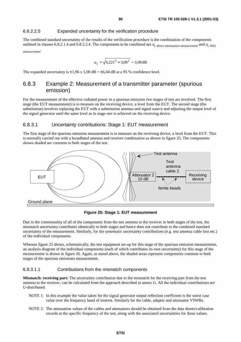
ETSI
ETSI TR 100 028-1 V1.3.1 (2001-03)90
6.8.2.2.5 Expanded uncertainty for the verification procedure
The combined standard uncertainty of the results of the verification procedure is the combination of the componentsoutlined in clauses 6.8.2.1.4 and 6.8.2.2.4. The components to be combined are uc direct attenuation measurement and uc NSA
measurement.
dB3,08=08,3221,0 22 +=cu
The expanded uncertainty is ±1,96 x 3,08 dB = ±6,04 dB at a 95 % confidence level.
6.8.3 Example 2: Measurement of a transmitter parameter (spuriousemission)
For the measurement of the effective radiated power in a spurious emission two stages of test are involved. The firststage (the EUT measurement) is to measure on the receiving device, a level from the EUT. The second stage (thesubstitution) involves replacing the EUT with a substitution antenna and signal source and adjusting the output level ofthe signal generator until the same level as in stage one is achieved on the receiving device.
6.8.3.1 Uncertainty contributions: Stage 1: EUT measurement
The first stage of the spurious emission measurement is to measure on the receiving device, a level from the EUT. Thisis normally carried out with a broadband antenna and receiver combination as shown in figure 25. The componentsshown shaded are common to both stages of the test.
Testantennacable 2
Test antenna
ferrite beads
Attenuator 210 dB
ReceivingdeviceEUT
Ground plane
Figure 25: Stage 1: EUT measurement
Due to the commonality of all of the components from the test antenna to the receiver in both stages of the test, themismatch uncertainty contributes identically to both stages and hence does not contribute to the combined standarduncertainty of the measurement. Similarly, for the systematic uncertainty contributions (e.g. test antenna cable loss etc.)of the individual components.
Whereas figure 25 shows, schematically, the test equipment set-up for this stage of the spurious emission measurement,an analysis diagram of the individual components (each of which contributes its own uncertainty) for this stage of themeasurement is shown in figure 26. Again, as stated above, the shaded areas represent components common to bothstages of the spurious emissions measurement.
6.8.3.1.1 Contributions from the mismatch components
Mismatch: receiving part: The uncertainty contribution due to the mismatch for the receiving part from the testantenna to the receiver, can be calculated from the approach described in annex G. All the individual contributions areU-distributed.
NOTE 1: In this example the value taken for the signal generator output reflection coefficient is the worst casevalue over the frequency band of interest. Similarly for the cable, adapter and attenuator VSWRs.
NOTE 2: The attenuation values of the cables and attenuators should be obtained from the data sheets/calibrationrecords at the specific frequency of the test, along with the associated uncertainties for these values.
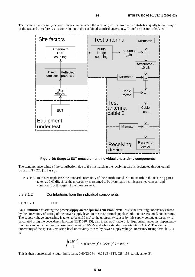
ETSI
ETSI TR 100 028-1 V1.3.1 (2001-03)91
The mismatch uncertainty between the test antenna and the receiving device however, contributes equally to both stagesof the test and therefore has no contribution to the combined standard uncertainty. Therefore it is not calculated.
Test antennaSite factors
Cablefactor
Testantennacable 2
Cableloss
Attenuator 210 dB
Equipmentunder test
Mismatch
Mutualimage
coupling
Antennagain +
Antenna toEUT
coupling
Reflectedpath loss
Directpath loss
Siteeffects
EUT
+
Receivingdevice
deviceReceiving
Mismatch
Mismatch +
+
Figure 26: Stage 1: EUT measurement individual uncertainty components
The standard uncertainty of the contribution, due to the mismatch in the receiving part, is designated throughout allparts of ETR 273 [12] as uj37.
NOTE 3: In this example case the standard uncertainty of the contribution due to mismatch in the receiving part istaken as 0,00 dB, since the uncertainty is assumed to be systematic i.e. it is assumed constant andcommon to both stages of the measurement.
6.8.3.1.2 Contributions from the individual components
6.8.3.1.2.1 EUT
EUT: influence of setting the power supply on the spurious emission level: This is the resulting uncertainty causedby the uncertainty of setting of the power supply level. In this case normal supply conditions are assumed, not extreme.The supply voltage uncertainty is taken to be ±100 mV so the uncertainty caused by this supply voltage uncertainty iscalculated using the dependency function (ETR 028 [15], part 2, annex C, table C.1: "Equipment under test dependencyfunctions and uncertainties") whose mean value is 10 %/V and whose standard uncertainty is 3 %/V. The standarduncertainty of the spurious emission level uncertainty caused by power supply voltage uncertainty (using formula 5.3)is:
%,=))%/V+()%/V(()V,(
6003103
10 222
×
This is then transformed to logarithmic form: 0,60/23,0 % = 0,03 dB (ETR 028 [15], part 2, annex E).

ETSI
ETSI TR 100 028-1 V1.3.1 (2001-03)92
The standard uncertainty of the contribution, due to the influence of setting the power supply on the spurious emissionlevel, is designated throughout all parts of ETR 273 [15] as uj54.
NOTE 1: In this example case the standard uncertainty of the contribution, due to the influence of setting the powersupply on the spurious emission level, is calculated above as 0,03 dB.
EUT: influence of the ambient temperature on the spurious emissions: This is the uncertainty in the power level ofthe spurious emission caused by the uncertainty in knowing the ambient temperature. The ambient temperatureuncertainty is ±1°C. The uncertainty caused by this temperature uncertainty is calculated using the dependency function(ETR 028 [15], part 2, annex C, table C.1: "EUT dependency functions and uncertainties") whose mean value is 4 %/°Cand whose standard uncertainty is 1,2 %/°C. The standard uncertainty of the spurious emission power level uncertaintycaused by ambient temperature uncertainty (using formula 5.3) is:
=))C%/,+()C%/,(()C)(
( 222
21043
1 °°×°2,41 %.
This is then transformed to logarithmic form: 2,41/23,0 % = 0,10 dB (ETR 028 [15]: part 2: annex E).
The standard uncertainty of the contribution, due to the influence of the ambient temperature on the spurious emissions,is designated throughout all parts of ETR 273 [12] as uj51.
NOTE 2: In this example case the standard uncertainty of the contribution due to the influence of the ambienttemperature on the spurious emissions level is calculated above as 0,10 dB.
EUT: mutual coupling to the power leads: This is the uncertainty associated with the influence (reflections, parasiticeffects, etc.) of the power leads on the EUT. The standard uncertainty associated with this effect is 0,5 dB provided thatthe precautions detailed in the methods have been observed. I.e. routing and dressing of cables with ferrites. If noprevention has been attempted the standard uncertainty is 2,0 dB. The standard uncertainty of the contribution, due tothe mutual coupling to the power leads, is designated throughout all parts of ETR 273 [12] as uj54.
NOTE 3: In this example case the standard uncertainty of the contribution due to the mutual coupling to the powerleads is taken as 0,5 dB since the precautions detailed in the methods are assumed to have been observed.
Position of the phase centre: within the EUT volume: This contribution is associated with the uncertainty with whichthe actual radiating point within the equipment volume is known. If this point is known exactly the contribution is0,00 dB. The standard uncertainty of the contribution, due to the position of the phase centre within the EUT volume, isdesignated throughout all parts of ETR 273 [12] as uj20.
NOTE 4: In this example case the standard uncertainty of the contribution due to the position of the phase centrewithin the EUT volume has been calculated from (±(the maximum dimension of device)/(2 × rangelength) × 100 %). In this example the position is not known. Hence, the uncertainty of the position of thephase centre within the EUT of 0,15 m maximum dimension is 0,15/2 m = 0,075 m, and the worst caseuncertainty due to this offset is therefore ±(0,075/3,0) × 100 % = ±2,50 %. As the phase centre can beanywhere inside the EUT, the uncertainty is taken as rectangularly distributed and the standarduncertainty is calculated as 1,44 %. This is then transformed to the logarithmic form(1,44/11,5) = 0,12 dB (ETR 028 [15]: part 2: annex E).
Positioning of the phase centre: within the EUT over the axis of rotation of the turntable: This contribution isassociated with the uncertainty with which the actual radiating point within the equipment is placed over the centre ofthe turntable. If the point is placed exactly, the contribution is 0,00 dB. The standard uncertainty of the contribution dueto the positioning of the EUT phase centre over the axis of rotation of the turntable, is designated throughout all parts ofETR 273 [12] as uj21.
NOTE 5: In this example case the standard uncertainty of the contribution due to the positioning of the EUT phasecentre over the axis of rotation of the turntable is calculated from (± (the estimated offset from the axis ofrotation)/(2 × range length) × 100 %). In this case, the uncertainty of the positioning is taken as ±0,01 m,and the worst case uncertainty is ±(0,01/3,0) × 100 = ±0,333 %. As the offset can be anywhere betweenthe limits the uncertainty is rectangularly distributed and the standard uncertainty is calculated as0,192 %. This is then transformed to the logarithmic form (0,192/11,5) = 0,02 dB (ETR 028 [15]: part 2:annex E).

ETSI
ETSI TR 100 028-1 V1.3.1 (2001-03)93
Range length: This contribution is associated with the curvature of the phase front from the EUT to the test antenna.The standard uncertainty of the contribution due to the range length is designated throughout all parts of ETR 273 [12]as uj16. The standard uncertainty of the contribution should be obtained from table 14.
Table 14: Uncertainty contribution of the range length (verification)
Range length (i.e. the horizontal distancebetween phase centres)
Standard uncertainty of thecontribution
(d1+d2)2/4λ ≤ range length < (d1+d2)
2/2λ 1,26 dB(d1+d2)
2/2λ ≤ range length < (d1+d2)2/λ 0,30 dB
(d1+d2)2/λ ≤ range length < 2(d1+d2)
2/λ 0,10 dBrange length ≥ 2(d1+d2)
2/λ 0,00 dB
NOTE 6: In table 14, d1 and d2 are the maximum dimensions of the antennas.
NOTE 7: In this example case the standard uncertainty of the contribution due to the range length is taken as0,00 dB since the range length is ≥ 2 (d1+d2)2/λ.
6.8.3.1.2.2 Site factors
Ambient effect: Ambient effect is the uncertainty caused by local ambient signals raising the noise floor at themeasurement frequency. The standard uncertainty of the contribution, due to the ambient effect, is designatedthroughout all parts of ETR 273 [12] as uj34. The values of the standard uncertainty should be taken from table 15.
Table 15: Uncertainty contribution: Ambient effect
Receiving device noise floor(EUT OFF) is within:
Standard uncertainty ofthe contribution
3 dB of measurement 1,57 dB3 dB to 6 dB of measurement 0,80 dB6 dB to 10 dB of measurement 0,30 dB10 dB to 20 dB of measurement 0,10 dB20 dB or more of the measurement 0,00 dB
NOTE 1: In this example case the standard uncertainty of the contribution due to the ambient effect is taken as0,00 dB, since the chamber is assumed to be shielded.
Mutual coupling: amplitude effect of the test antenna on the EUT: This uncertainty results from the interactionbetween the EUT and the test antenna when placed close together. The standard uncertainty of the contribution due tothe amplitude effect of the mutual coupling between the test antenna and the EUT, is designated throughout all parts ofETR 273 [12] as uj08. The standard uncertainty should be taken from table 16.
Table 16: Uncertainty contribution: Mutual coupling: amplitude effectof the test antenna on the EUT
Range length Standard uncertainty of the contribution0,62√((d1+d2)
3/λ)≤ range length < 2(d1+d2)2/λ 0,50 dB
range length ≥ 2(d1+d2)2/λ 0,00 dB
NOTE 2: In this example case the standard uncertainty of the contribution due to the amplitude effect of the mutualcoupling between the test antenna and the EUT is 0,00 dB since the distance is ≥ 2 (d1+d2)2/λ.
Mutual coupling: EUT to its images in the absorbing material: This uncertainty is dependant on the quality of theabsorbing material and the effect imaging of the EUT in the ceiling, side and end walls has on the input impedanceand/or gain of the integral antenna. The standard uncertainty of the contribution, due to the mutual coupling of the EUTto its images in the absorbing material, is designated throughout all parts of ETR 273 [12] as uj04.
NOTE 3: In this example case the standard uncertainty of the contribution due to the mutual coupling amplitudeeffect of the absorbing material on the EUT is assumed to be 0,5 dB (see annex A).

ETSI
ETSI TR 100 028-1 V1.3.1 (2001-03)94
Mutual coupling: EUT to its image in the ground plane: This uncertainty results from the change in the EUTspurious emission level as a result of being placed close to the ground plane. The standard uncertainty of thecontribution, due to the mutual coupling of the EUT to its image in the ground plane, is designated throughout all partsof ETR 273 [12] as uj13. Its value can be obtained from table 17.
Table 17: Uncertainty contribution of the mutual coupling betweenthe EUT to its image in the ground plane
Spacing between the EUTand the ground plane
Standard uncertaintyof the contribution
For a vertically polarized EUTspacing ≤ 1,25 λ 0,15 dBspacing > 1,25 λ 0,06 dB
For a horizontally polarized EUTspacing < λ/2 1,15 dB
λ/2 ≤ spacing < 3λ/2 0,58 dB3λ/2 ≤ spacing < 3λ 0,29 dB
spacing ≥ 3λ 0,15 dB
NOTE 4: In this example case the standard uncertainty of the contribution, due to the mutual coupling of the EUTto its image in the ground plane (assuming the polarization is vertical and the spacing above the groundplane is < 1,25 λ at the test frequency), is taken as 0,15 dB.
Reflectivity of absorbing material: EUT to the test antenna. This uncertainty is associated with the magnitudes ofthe reflections occurring from the side walls, end walls and ceiling. These magnitudes are a function of the quality ofthe absorber at the frequency of test. The standard uncertainty of the contribution, due to the reflectivity of theabsorbing material between the EUT and the test antenna, is designated throughout all parts of ETR 273 [12] as uj01.
The relevant value for this contribution should be taken from table 18.
Table 18: Uncertainty contribution of the reflectivityof absorbing material between the EUT and test antenna
Reflectivity of the absorbing material Standard uncertainty of the contributionreflectivity <10 dB 4,76 dB10 ≤ reflectivity < 15 dB 3,92 dB15 ≤ reflectivity < 20 dB 2,56 dB20 ≤ reflectivity < 30 dB 1,24 dBreflectivity ≥ 30 dB 0,74 dB
NOTE 5: In this example case the standard uncertainty of the contribution due to the reflectivity of the absorbingmaterial between the EUT and the test antenna is taken as 0,00 dB since this is a substitutionmeasurement and the contribution cancels (see annex A).
Mutual coupling: test antenna to its images in the absorbing material: This is the uncertainty due to the mutualcoupling between the test antenna and its images in the ceiling, side and end walls and is the effect of the changeproduced in the antenna's input impedance and/or gain. As this is the first stage of a substitution measurement and theuncertainty is common to both stages it will only contribute in the second stage if the test antenna is located at adifferent height on the antenna mast. The standard uncertainty of the contribution, due to the mutual coupling betweenthe test antenna and its images in the absorbing material, is designated throughout all parts of ETR 273 [12] as uj06.
NOTE 6: In this example case the standard uncertainty of the contribution due to the mutual coupling between thetest antenna and its images in the absorbing material is taken as 0,00 dB since this is the referenceposition.
Mutual coupling: test antenna to its image in the ground plane: This is the uncertainty due to the mutual couplingbetween the test antenna and its image in the ground plane and is the effect of the change produced in the antenna'sinput impedance and/or gain when placed close to a ground plane. As this is the first stage of a substitutionmeasurement and the uncertainty is common to both stages, it will only contribute in the second stage if the test antennais located at a different height on the antenna mast. The standard uncertainty of the contribution, due to the mutualcoupling between the test antenna and its image in the ground plane, is designated throughout all parts of ETR 273 [12]as uj14.

ETSI
ETSI TR 100 028-1 V1.3.1 (2001-03)95
NOTE 7: In this example case the standard uncertainty of the contribution due to the mutual coupling between thetest antenna and its image in the ground plane is taken as 0,00 dB since this is the reference position.
6.8.3.1.2.3 Test antenna
Correction: measurement distance: For those tests in which the test antenna on the mast peaks at different heights inthe two stages, a correction for the measurement distance should be made to account for the different measurementdistances. The standard uncertainty of the contribution due to the correction for measurement distance is designatedthroughout all parts of ETR 273 [12] as uj18.
NOTE 1: In this example case the standard uncertainty of the contribution due to the correction for measurementdistance is taken as 0,00 dB since, in this, the first stage of the measurement, only a reference height isbeing set.
Correction: off boresight angle in elevation plane: For those tests in which the test antenna on the mast peaks atdifferent heights in the two stages, a correction must be made to account for the different angles subtended by theEUT/substitution antenna. The standard uncertainty of the contribution, due to the correction for off boresight angle inelevation plane, is designated throughout all parts of ETR 273 [12] as uj17.
NOTE 2: In this example case the standard uncertainty of the contribution due to the correction for off boresightangle in elevation plane is taken as 0,00 dB since in this, the first stage of the measurement, only areference height is being set.
Antenna: gain of the test antenna: The gain, and its uncertainty, of the test antenna act as systematic offsets since theyare present in both stages of the test. The standard uncertainty of the contribution, due to the uncertainty of the gain ofthe test antenna, is designated throughout all parts of ETR 273 [12] as uj45.
NOTE 3: In this example case the standard uncertainty of the contribution due to the uncertainty of the gain of thetest antenna is taken as 0,00 dB since the uncertainty is systematic i.e. it produces the same offset in bothstages.
Antenna: tuning of the test antenna: This uncertainty is introduced as a result of inaccurate tuning of the test antenna.The standard uncertainty of the contribution, due to the tuning of the test antenna, is designated throughout all parts ofETR 273 [12] as uj46.
NOTE 4: In this example case the standard uncertainty of the contribution due to the tuning of the test antenna istaken as 0,00 dB since the uncertainty is systematic i.e. it is assumed constant and common to both stagesof the measurement and, provided that once set in stage one of the test it is not subsequently re-tuned, itscontribution is the same in both stages.
Position of the phase centre: test antenna: The horizontal position of the test antenna defines one end of the rangelength. The standard uncertainty of the contribution, due to the position of the phase centre of the test antenna, isdesignated throughout all parts of ETR 273 [12] as uj22.
NOTE 5: In this example case the test antenna is assumed to describe a vertical straight line as its height on themast is changed. The standard uncertainty of the contribution due to the position of the phase centre of thetest antenna is assumed to be 0,00 dB (see annex A).
6.8.3.1.2.4 Test antenna attenuator
Insertion loss: test antenna attenuator: The attenuator has an insertion loss as well as an uncertainty associated withthe measurement of its magnitude. The value of insertion loss and its uncertainty remain valid provided the attenuator isnot used outside the manufacturer's specification. At any given frequency the insertion loss acts as a systematic offsetand contributes equally to both stages of the measurement. The standard uncertainty of the contribution due to theinsertion loss of the test antenna attenuator is designated throughout all parts of ETR 273 [12] as uj40.
NOTE: In this example case the standard uncertainty of the contribution, due to the insertion loss uncertainty ofthe test antenna attenuator, is taken as 0,00 dB since the uncertainty is systematic i.e. it produces the sameoffset in both stages.
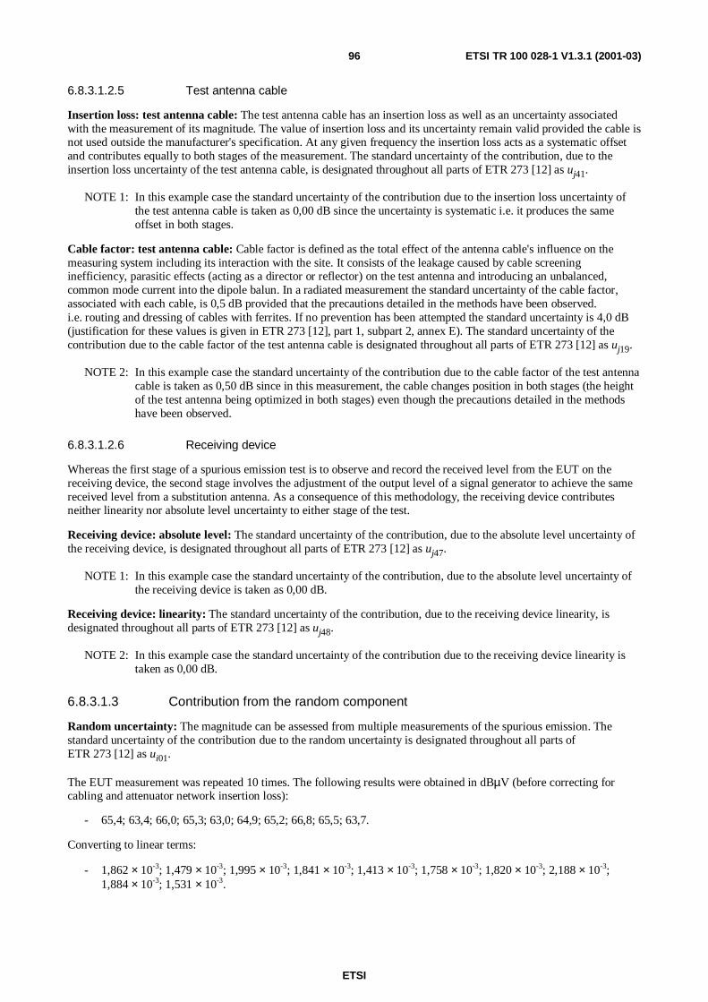
ETSI
ETSI TR 100 028-1 V1.3.1 (2001-03)96
6.8.3.1.2.5 Test antenna cable
Insertion loss: test antenna cable: The test antenna cable has an insertion loss as well as an uncertainty associatedwith the measurement of its magnitude. The value of insertion loss and its uncertainty remain valid provided the cable isnot used outside the manufacturer's specification. At any given frequency the insertion loss acts as a systematic offsetand contributes equally to both stages of the measurement. The standard uncertainty of the contribution, due to theinsertion loss uncertainty of the test antenna cable, is designated throughout all parts of ETR 273 [12] as uj41.
NOTE 1: In this example case the standard uncertainty of the contribution due to the insertion loss uncertainty ofthe test antenna cable is taken as 0,00 dB since the uncertainty is systematic i.e. it produces the sameoffset in both stages.
Cable factor: test antenna cable: Cable factor is defined as the total effect of the antenna cable's influence on themeasuring system including its interaction with the site. It consists of the leakage caused by cable screeninginefficiency, parasitic effects (acting as a director or reflector) on the test antenna and introducing an unbalanced,common mode current into the dipole balun. In a radiated measurement the standard uncertainty of the cable factor,associated with each cable, is 0,5 dB provided that the precautions detailed in the methods have been observed.i.e. routing and dressing of cables with ferrites. If no prevention has been attempted the standard uncertainty is 4,0 dB(justification for these values is given in ETR 273 [12], part 1, subpart 2, annex E). The standard uncertainty of thecontribution due to the cable factor of the test antenna cable is designated throughout all parts of ETR 273 [12] as uj19.
NOTE 2: In this example case the standard uncertainty of the contribution due to the cable factor of the test antennacable is taken as 0,50 dB since in this measurement, the cable changes position in both stages (the heightof the test antenna being optimized in both stages) even though the precautions detailed in the methodshave been observed.
6.8.3.1.2.6 Receiving device
Whereas the first stage of a spurious emission test is to observe and record the received level from the EUT on thereceiving device, the second stage involves the adjustment of the output level of a signal generator to achieve the samereceived level from a substitution antenna. As a consequence of this methodology, the receiving device contributesneither linearity nor absolute level uncertainty to either stage of the test.
Receiving device: absolute level: The standard uncertainty of the contribution, due to the absolute level uncertainty ofthe receiving device, is designated throughout all parts of ETR 273 [12] as uj47.
NOTE 1: In this example case the standard uncertainty of the contribution, due to the absolute level uncertainty ofthe receiving device is taken as 0,00 dB.
Receiving device: linearity: The standard uncertainty of the contribution, due to the receiving device linearity, isdesignated throughout all parts of ETR 273 [12] as uj48.
NOTE 2: In this example case the standard uncertainty of the contribution due to the receiving device linearity istaken as 0,00 dB.
6.8.3.1.3 Contribution from the random component
Random uncertainty: The magnitude can be assessed from multiple measurements of the spurious emission. Thestandard uncertainty of the contribution due to the random uncertainty is designated throughout all parts ofETR 273 [12] as ui01.
The EUT measurement was repeated 10 times. The following results were obtained in dBµV (before correcting forcabling and attenuator network insertion loss):
- 65,4; 63,4; 66,0; 65,3; 63,0; 64,9; 65,2; 66,8; 65,5; 63,7.
Converting to linear terms:
- 1,862 × 10-3; 1,479 × 10-3; 1,995 × 10-3; 1,841 × 10-3; 1,413 × 10-3; 1,758 × 10-3; 1,820 × 10-3; 2,188 × 10-3;1,884 × 10-3; 1,531 × 10-3.

ETSI
ETSI TR 100 028-1 V1.3.1 (2001-03)97
The two sums X and Y are calculated:
- X = the sum of the measured values = 17,77 × 10⁻³;
- Y = the sum of the squares of the measured values = 32,10 × 10⁻⁶ V2.
( )=
−
×−×=
−
−=
−−
11010
1077,171010,32
1
236
2
nn
XY
uc random 238,3 ×10⁻⁶ (formula 5.6)
As the result is obtained as the mean value of 10 measurements and the standard uncertainty of the random uncertaintyis:
dB1,175,11
100
10777,1
103,2383
6=×
×
×=−
−
j randomu
NOTE: In this example case the standard uncertainty of the contribution due to the random uncertainty is 1,17 dB.
6.8.3.1.4 Summary table of contributory components
All the uncertainty contributions for this part of the procedure are listed in table 19.
Table 19: Contributions from the EUT measurement
uj or i Description of uncertainty contributions dBuj37 mismatch: receiving part 0,00uj54 EUT: influence of setting the power supply on the spurious emission level 0,03uj51 EUT: influence of the ambient temperature on the spurious emission level 0,03uj55 EUT: mutual coupling to the power leads 0,50uj20 position of the phase centre: within the EUT volume 0,12uj21 positioning of the phase centre: within the EUT over the axis of rotation of the turntable 0,02uj16 range length 0,00uj34 ambient effect 0,00uj08 mutual coupling: amplitude effect of the test antenna on the EUT 0,00uj04 Mutual coupling: EUT to its images in the absorbing material 0,50uj13 mutual coupling: EUT to its image in the ground plane 0,15uj01 reflectivity of absorbing material: EUT to the test antenna 0,00uj06 mutual coupling: test antenna to its images in the absorbing material 0,00uj14 mutual coupling: test antenna to its image in the ground plane 0,00uj18 correction: measurement distance 0,00uj17 correction: off boresight angle in elevation plane 0,00uj45 antenna: gain of the test antenna 0,00uj46 antenna: tuning of the test antenna 0,00uj22 position of the phase centre: test antenna 0,00uj40 insertion loss: test antenna attenuator 0,00uj41 insertion loss: test antenna cable 0,00uj19 cable factor: test antenna cable 0,50uj47 receiving device: absolute level 0,00uj48 receiving device: linearity 0,00ui01 random uncertainty 1,17
The standard uncertainties from table 19 should be combined by RSS in accordance with ETR 273 [12], part 1,subpart 1, clause 5. This gives the combined standard uncertainty (uc contribution from the EUT measurement) for the EUTmeasurement in dB.
The value of uc contribution from the EUT measurement is calculated as 1,47 dB.

ETSI
ETSI TR 100 028-1 V1.3.1 (2001-03)98
6.8.3.2 Uncertainty contributions: Stage 2: Substitution measurement
The second stage of the spurious emission test (the substitution) involves replacing the EUT with a substitution antennaand signal source as shown in figure 27, and adjusting the output level of the signal generator until the same level as instage one is achieved on the receiving device.
Ground plane
Testantennacable 2
Test antenna
ferrite beads
Attenuator 210 dB
Receivingdevice
cable 1
ferrite beads
Attenuator 110 dB
Signalgenerator
Figure 27: Stage two: Typical emission substitution test
Whereas figure 27 shows, schematically, the test equipment set-up for this substitution stage of the spurious emissiontest, figure 28, an analysis diagram, provides a detailed picture of the individual uncertainty components (each of whichcontributes its own uncertainty) for this stage in the measurement. As stated above, the shaded areas representcomponents common to both stages of the test method.
6.8.3.2.1 Contributions from the mismatch components
Mismatch uncertainty transmitting and receiving parts: The value of the combined standard uncertainty of thecontribution due to the mismatch for the substitution measurement are calculated from the approach described inannex G. For this stage it is calculated in two parts. Firstly the standard uncertainty of the contribution due to themismatch in the transmitting part, i.e. between the signal generator, cable, attenuator and the substitution antenna andsecondly, that for the receiving part, i.e. between the test antenna, attenuator, cable and the receiver. However, only thecontribution for the transmitting part is actually calculated since the receiving part is common to both stages of the testand its uncertainty contribution therefore largely cancels.
Mismatch: transmitting part:
Signal generator: Output reflection coefficient: |ρG| = 0,20
Cable: Input and output reflection coefficients: |S11| and |S22| = 0,07
Attenuation: 1 dB = |S12| = |S21| = 0,891
Attenuator: Input and output reflection coefficients |S11| = |S22| = 0,05
Attenuation = 10 dB |S12| = |S21| = 0,3162
Transmitting antenna: Input reflection coefficient: |ρTA| = 0,333
All these contributions are U-distributed. Those components that cancel are not calculated. Other contributions are (seeannex G):
- uj generator and cable 1: Constant for both stage 1 and 2. Hence this value does not contribute.
- uj cable 1 and attenuator 1: Constant for both stage 1 and 2. Hence this value does not contribute.
%177,1%2
100333,005,01 =××=antennaandattenuatorju
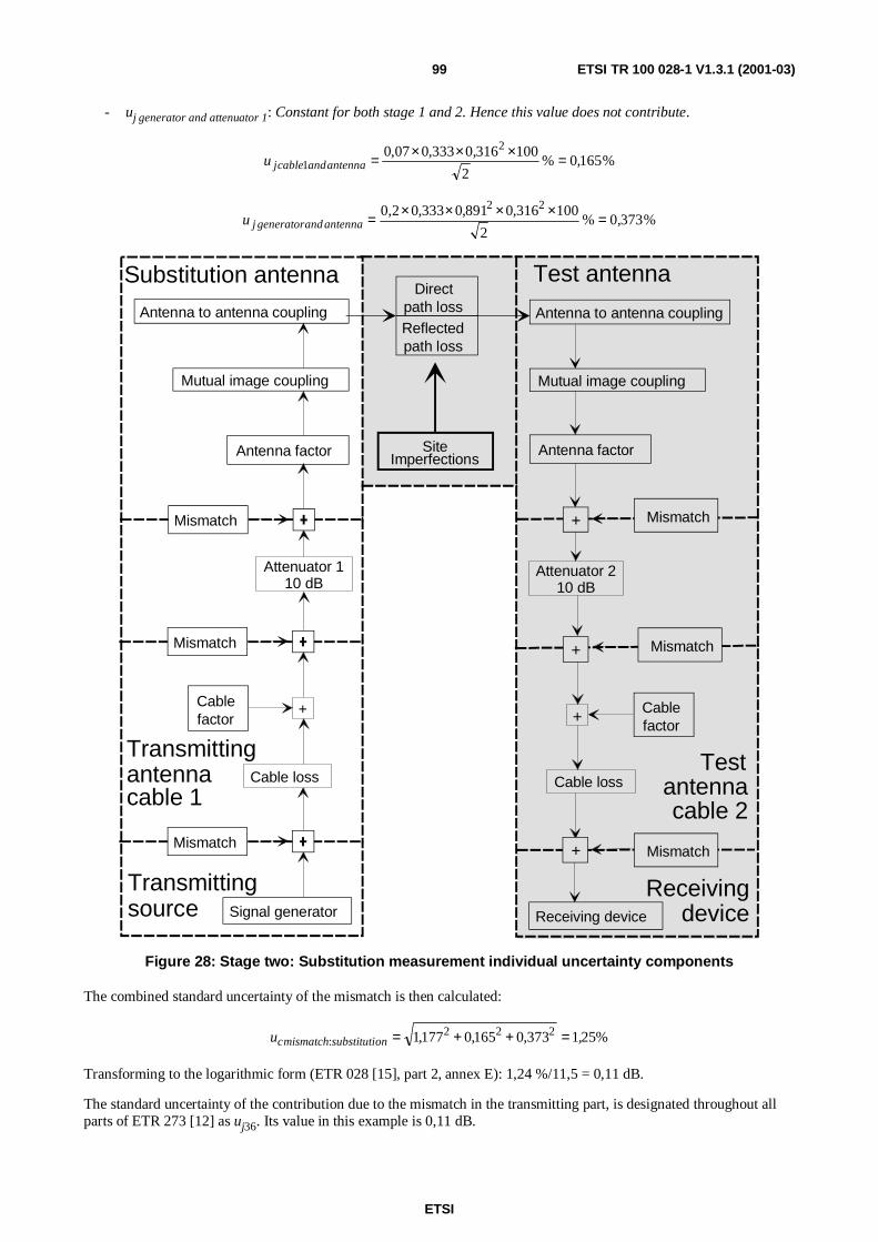
ETSI
ETSI TR 100 028-1 V1.3.1 (2001-03)99
- uj generator and attenuator 1: Constant for both stage 1 and 2. Hence this value does not contribute.
%165,0%2
100316,0333,007,0 2
1 =×××=antennaandcableju
%373,0%2
100316,0891,0333,02,0 22=××××=antennaandgeneratorju
Substitution antenna
Cablefactor
Test antenna
Cablefactor+
Antenna to antenna coupling
Mutual image coupling
Antenna factor
Cable loss
Directpath lossReflectedpath loss
SiteImperfections
Antenna to antenna coupling
Mutual image coupling
Antenna factor
Mismatch
Mismatch
+
Cable loss
Mismatch
Signal generator Receiving device
Testantennacable 2
Receivingdevice
Transmittingantennacable 1
Transmittingsource
Attenuator 110 dB
Attenuator 210 dB
Mismatch
Mismatch
Mismatch+
+
+
Figure 28: Stage two: Substitution measurement individual uncertainty components
The combined standard uncertainty of the mismatch is then calculated:
%251373,0165,0177,1 222: ,u onsubstitutimismatchc =++=
Transforming to the logarithmic form (ETR 028 [15], part 2, annex E): 1,24 %/11,5 = 0,11 dB.
The standard uncertainty of the contribution due to the mismatch in the transmitting part, is designated throughout allparts of ETR 273 [12] as uj36. Its value in this example is 0,11 dB.

ETSI
ETSI TR 100 028-1 V1.3.1 (2001-03)100
Mismatch: Receiving part:
The mismatch uncertainty between the test antenna and the receiving device contributes equally to both stages of thetest and therefore has no contribution to the combined standard uncertainty. Therefore it is not calculated. The standarduncertainty of the contribution due to mismatch in the receiving part is designated throughout all parts of ETR 273 [12]as uj37.
NOTE 4: In this example case the standard uncertainty of the contribution due to mismatch in the receiving part istaken as 0,00 dB since the uncertainty is systematic i.e. it produces the same offset in both stages.
6.8.3.2.2 Contributions from the individual components
6.8.3.2.2.1 Signal generator
Signal generator: absolute output level: The signal generator replaces the EUT in the substitution part of this test and,as a result, should be included in the combined standard uncertainty since it does not cancel as a systematic offset. Thestandard uncertainty of the contribution, due to the signal generator absolute output level, is designated throughout allparts of ETR 273 [12] as uj38.
NOTE 1: In this example case the uncertainty of the contribution due to the signal generator absolute output leveluncertainty is obtained from the manufacturers data sheet as ±1,0 dB. As nothing is said about thedistribution of this uncertainty, a rectangular distribution (see ETR 273 [12], part 1, subpart 1,clause 5.1.2) in logs is assumed, and the standard uncertainty is calculated as 0,58 dB.
Signal generator: output level stability: In any test in which the contribution of the absolute level uncertainty of thesignal generator contributes to the combined standard uncertainty of the test i.e. it does not cancel due to themethodology, the contribution from the output level stability is considered to have been included in the signal generatorabsolute output level, uj38. Conversely, for any level in which the absolute level uncertainty of the signal generator does
not contribute to the combined standard uncertainty, the output level stability of the signal generator should be included.The standard uncertainty of the contribution due to the signal generator output level stability is designated throughoutall parts of ETR 273 [12] as uj39. Its value can be derived from manufacturers' data sheet.
NOTE 2: In this example case the standard uncertainty of the contribution due to the signal generator output levelstability is taken as 0,00 dB as it is covered by the absolute level uncertainty.
6.8.3.2.2.2 Substitution antenna cable
Insertion loss: substitution antenna cable: The substitution antenna cable has an insertion loss as well as anuncertainty associated with the measurement of its magnitude. The value of insertion loss and its uncertainty remainvalid provided the cable is not used outside the manufacturer's specification. At any given frequency the insertion lossacts as a systematic offset and contributes equally to both stages of the measurement. The standard uncertainty of thecontribution due to the insertion loss uncertainty of the substitution antenna cable, is designated throughout all parts ofETR 273 [12] as uj41.
NOTE 1: In this example case the uncertainty of the contribution due to the insertion loss uncertainty of thesubstitution antenna cable is taken from the manufacturers data sheet as ±0,5 dB. As nothing is said aboutthe distribution, a rectangular distribution (see ETR 273 [12], part 1, subpart 1, clause 5.1.2) in logs isassumed and the standard uncertainty is calculated as 0,29 dB.
Cable factor: substitution antenna cable: Cable factor is defined as the total effect of the antenna cable's influence onthe measuring system including its interaction with the site. It consists of the leakage caused by cable screeninginefficiency, parasitic effects (acting as a director or reflector) and introducing an unbalanced, common mode currentinto the dipole balun. In a radiated measurement the standard uncertainty of the cable factor, associated with thesubstitution antenna cable is 0,5 dB provided the precautions detailed in the methods have been observed. i.e. routingand dressing of cables with ferrites. If no prevention has been attempted the standard uncertainty is 4,0 dB (justificationfor these values is given in ETR 273 [12], part 1, subpart 2, annex E). The standard uncertainty of the contribution, dueto the cable factor of the substitution antenna cable, is designated throughout all parts of ETR 273 [12] as uj19.
NOTE 2: In this example case the standard uncertainty of the contribution due to the cable factor of the substitutionantenna cable is taken as 0,50 dB since the precautions detailed in the methods are assumed to have beenobserved.

ETSI
ETSI TR 100 028-1 V1.3.1 (2001-03)101
6.8.3.2.2.3 Substitution antenna attenuator
Insertion loss: substitution antenna attenuator: The attenuator has an insertion loss as well as an uncertaintyassociated with the measurement of its magnitude. The value of insertion loss and its uncertainty remain valid providedthe attenuator is not used outside the manufacturer's specification. At any given frequency the insertion loss is takenfrom the manufacturer's data sheet since it does not cancel as a systematic offset (it only appears in one stage of thetest). The standard uncertainty of the contribution, due to the insertion loss uncertainty of the substitution antennaattenuator, is designated throughout all parts of ETR 273 [12] as uj40.
NOTE : In this example case the uncertainty of the contribution, due to the insertion loss uncertainty of thesubstitution antenna attenuator, is obtained from the manufacturer's data sheet as ±0,3 dB. As nothing issaid about the distribution, a rectangular distribution (see ETR 273 [12], part 1, subpart 1, clause 5.1.2) inlogs is assumed and the standard uncertainty is calculated as 0,17 dB.
6.8.3.2.2.4 Substitution antenna
Antenna: gain of the substitution antenna: The gain (and its uncertainty) of the substitution antenna is only involvedin the second stage of the test. The standard uncertainty of the contribution due to the gain of the substitution antenna isdesignated throughout all parts of ETR 273 [12] as uj45. For ANSI dipoles the value should be obtained from table 20.
Table 20: Uncertainty contribution: Antenna: gain of the test or substitution antenna
Frequency Standard uncertainty of thecontribution
30 MHz ≤ frequency ≤ 80 MHz 1,73 dB80 MHz < frequency ≤ 180 MHz 0,60 dBfrequency > 180 MHz 0,30 dB
NOTE 1: For other antenna types the figures should be taken from manufacturers data sheets. If a figure is notgiven the standard uncertainty is 1,0 dB.
NOTE 2: In this example case the standard uncertainty of the contribution due to the gain of the substitutionantenna is taken as 0,3 dB as an ANSI dipole is used and the frequency is above 180 MHz.
Antenna: tuning of the substitution antenna: Uncertainty is introduced as a result of the inaccurate tuning of thesubstitution antenna. This only occurs in stage two of the measurement. The standard uncertainty of the contribution,due to the tuning of the substitution antenna, is designated throughout all parts of ETR 273 [12] as uj46.
NOTE 3: In this example case the standard uncertainty of the contribution due to the tuning of the substitutionantenna is taken as 0,06 dB.
Position of the phase centre: substitution antenna: Uncertainty is introduced as a result of the inaccurate positioningof the phase centre of the substitution antenna. This only occurs in stage two of the measurement. The standarduncertainty of the contribution, due to the position of the phase centre of the substitution antenna, is designatedthroughout all parts of ETR 273 [12] as uj22.
NOTE 4: In this example case the standard uncertainty of the contribution due to the uncertainty in the position ofthe phase centre of the substitution antenna has been calculated from (±(the offset from axis of rotation)/(range length) x100 %). The positioning uncertainty is ±0,01 m and therefore the worst case uncertainty= 0,01/3,0 = 0,333 %. As the offset can be anywhere between these limits, the uncertainty is taken to berectangularly distributed (see ETR 273 [12], part 1, subpart 1, clause 5.1.2) and the standard uncertainty iscalculated as 0,192 %. This is transformed to the logarithmic form (ETR 028 [15], part 2, annex E), to be0,02 dB.

ETSI
ETSI TR 100 028-1 V1.3.1 (2001-03)102
6.8.3.2.2.5 Site factors
Ambient effect: Uncertainty is introduced as a result of local ambient signals raising the noise floor at the measurementfrequency. The standard uncertainty of the contribution due to the ambient effect is designated throughout all parts ofETR 273 [12] as uj34. The values of the standard uncertainty should be taken from table 21.
Table 21: Uncertainty contribution: Ambient effect
Receiving device noise floor(generator OFF) is within:
Standard uncertainty ofthe contribution
3 dB of measurement 1,57 dB3 dB to 6 dB of measurement 0,80 dB6 dB to 10 dB of measurement 0,30 dB10 dB to 20 dB of measurement 0,10 dB20 dB or more of the measurement 0,00 dB
NOTE 1: In this example case the standard uncertainty of the contribution due to the ambient effect is taken as0,00 dB, since the chamber is assumed to be shielded.
Mutual coupling: substitution antenna to its images in the absorbing material: This uncertainty is the effect of thechange produced in the antenna's input impedance and/or gain. The standard uncertainty of the contribution due to themutual coupling of the substitution antenna to its images in the absorbing material is designated throughout all parts ofETR 273 [12] as uj06.
NOTE 2: In this example case the standard uncertainty of the contribution due to the mutual coupling of thetransmitting antenna to its images in the absorbing materials is taken as 0,5 dB (see annex A).
Mutual coupling: substitution antenna to its image in the ground plane: This uncertainty is the effect of the changeproduced in the antenna's input impedance and/or gain. The standard uncertainty of the contribution due to the mutualcoupling of the substitution antenna to its image in the ground plane, designated throughout all parts of ETR 273 [12] asuj14. has a value of 0,00 dB for ANSI dipoles since it is included, where significant, in the mutual coupling andmismatch loss correction factors (see table A.20). For other dipoles the value can be obtained from table 22.
Table 22: Uncertainty contribution of the mutual coupling betweenthe substitution antenna and its image in the ground plane
Spacing between the antennaand the ground plane
Standard uncertaintyof the contribution
For a vertically polarized antennaspacing ≤ 1,25 λ 0,15 dBspacing > 1,25 λ 0,06 dB
For a horizontally polarized antennaspacing < λ/2 1,15 dB
λ/2 ≤ spacing < 3λ/2 0,58 dB3λ/2 ≤ spacing < 3λ 0,29 dB
spacing ≥ 3λ 0,15 dB
NOTE 3: In this example case the standard uncertainty of the contribution due to mutual coupling between thesubstitution antenna and its image in the ground plane is taken as 0,58 dB.
Mutual coupling: substitution antenna to the test antenna: This is the effect produced by any change in gain of theantennas which results from their close spacing. The standard uncertainty of the contribution due to the mutual couplingof the substitution antenna to the test antenna, designated throughout all parts of ETR 273 [12] as uj11. For ANSI
dipoles the value of this uncertainty is 0,00 dB as it is included, where significant, in the mutual coupling and mismatchloss correction factors. For non-ANSI dipoles the standard uncertainty for frequencies can be taken from table 23.

ETSI
ETSI TR 100 028-1 V1.3.1 (2001-03)103
Table 23: Uncertainty contribution of the mutual couplingbetween the substitution and test antennas
Frequency Standard uncertaintyof the contribution
(3 m range)
Standard uncertaintyof the contribution
(10 m range)30 MHz ≤ frequency < 80 MHz 1,73 dB 0,60 dB80 MHz ≤ frequency < 180 MHz 0,6 dB 0,00 dBfrequency ≥ 180 MHz 0,00 dB 0,00 dB
NOTE 4: In this example case the standard uncertainty of the contribution due to mutual coupling between thesubstitution and test antennas is taken as 0,00 dB as the frequency is above 180 MHz.
Mutual coupling: interpolation of mutual coupling and mismatch loss correction factors, only for ANSI dipoles:The standard uncertainty of the contribution due to the interpolation of mutual coupling and mismatch loss correctionfactors, is designated throughout all parts of ETR 273 [12] as uj12. For spot frequencies given in table A.20, the value ofthe contribution is 0,00 dB. However, for all other frequencies, the standard uncertainty should be obtained fromtable 24.
Table 24: Uncertainty contribution of the interpolationof mutual coupling and mismatch loss correction factors
Frequency (MHz) Standard uncertainty of the contributionfor a spot frequency given in the table 0,00 dB30 MHz ≤ frequency < 80 MHz 0,58 dB80 MHz ≤ frequency < 180 MHz 0,17 dBfrequency ≥ 180 MHz 0,00 dB
NOTE 5: In this example case the standard uncertainty of the contribution due to the interpolation of mutualcoupling and mismatch loss correction factors is taken as 0,00 dB as the frequency is above 180 MHz.
Range length: This contribution is associated with the curvature of the phase front from the substitution antenna to thetest antenna. The standard uncertainty of the contribution, due to range length, is designated throughout all parts ofETR 273 [12] as uj16. The standard uncertainty is 0,00 dB if ANSI dipoles are used. For other types of antenna thestandard uncertainty of the contribution should be obtained from table 25.
Table 25: Uncertainty contribution of the range length (verification)
Range length (i.e. the horizontal distancebetween phase centres)
Standard uncertainty of thecontribution
(d1+d2)2/4λ ≤ range length < (d1+d2)
2/2λ 1,26 dB(d1+d2)
2/2λ ≤ range length < (d1+d2)2/λ 0,30 dB
(d1+d2)2/λ ≤ range length < 2(d1+d2)
2/λ 0,10 dBrange length ≥ 2(d1+d2)
2/λ 0,00 dB
NOTE 6: In table 25, d1 and d2 are the maximum dimensions of the antennas.
NOTE 7: The standard uncertainty of the contribution due to the range length is taken as 0,00 dB since in this casethe range length is ≥ 2 (d1+d2)2/λ.
Reflectivity of absorbing material: substitution antenna to the test antenna: This uncertainty is associated with themagnitude of the reflections occurring from the side walls, end walls and ceiling. These magnitudes are a function ofthe quality of the absorber at the frequency of test. However, in this, a substitution measurement, the contribution isonly concerned with taking into account the possible differences in the antenna patterns (principally in the verticalplane) between the EUT and substitution antenna. The standard uncertainty of the contribution due to the reflectivity ofthe absorbing material between the substitution and test antenna is designated throughout all parts of ETR 273 [12] asuj02.
NOTE 8: In this example case the standard uncertainty of the contribution due to the reflectivity of the absorbingmaterial between the substitution and test antenna is 0,50 dB (see annex A).

ETSI
ETSI TR 100 028-1 V1.3.1 (2001-03)104
Mutual coupling: test antenna to its images in the absorbing material: This is the uncertainty due to the mutualcoupling between the test antenna and its images in the ceiling, side and end walls and is the effect of the changeproduced in the antenna's input impedance and/or gain. As this is the second stage of a substitution measurement andthe uncertainty is common to both stages it will only contribute in this stage if the test antenna is located at a differentheight on the antenna mast from the first stage. The standard uncertainty of the contribution, due to the mutual couplingof the test antenna to its images in the absorbing material, is designated throughout all parts of ETR 273 [12] as uj06.
NOTE 9: In this example case the standard uncertainty of the contribution due to the mutual coupling of the testantenna to its images in the absorbing material is taken as 0,50 dB since this is the second stage of asubstitution measurement and the test antenna is assumed to be located at a different height to stage oneand therefore the contribution does not cancel.
Mutual coupling: test antenna to its image in the ground plane: As this is the second stage of a substitutionmeasurement and the uncertainty is common to both stages it will only contribute in this stage if the test antenna islocated at a different height on the antenna mast from the first stage. The standard uncertainty of the contribution, due tothe mutual coupling of the test antenna to its image in the ground plane, is designated throughout all parts ofETR 273 [12] as uj14.
NOTE 10:In this example case the standard uncertainty of the contribution due to the mutual coupling of the testantenna to its image in the ground plane is taken as 0,50 dB since this is the second stage of a substitutionmeasurement and the test antenna is assumed to be located at a different height to stage one and thereforethe contribution does not cancel.
6.8.3.2.2.6 Test antenna
Correction: measurement distance: For those tests in which the test antenna on the mast peaks at different heights inthe two stages, a correction should be made to account for the different measurement distances. Where a correction isrequired the standard uncertainty of the correction factor should be taken as 0,10 dB. The standard uncertainty of thecontribution due to the correction for measurement distance is designated throughout all parts of ETR 273 [12] as uj18.
NOTE 1: In this example case the standard uncertainty of the contribution due to the correction for measurementdistance is taken as 0,10 dB since it is assumed that, in this second stage, a different height of test antennahas been necessary and the correction applied.
Correction: off boresight angle in elevation plane: For those tests in which the test antenna on the mast peaks atdifferent heights in the two stages, a correction should be made to account for the different angles subtended by theEUT/substitution antenna. Where a correction is required the standard uncertainty of the correction factor should betaken as 0,10 dB. The standard uncertainty of the contribution due to the correction for off boresight angle in elevationplane is designated throughout all parts of ETR 273 [12] as uj17.
NOTE 2: In this example case the standard uncertainty of the contribution due to the correction for off boresightangle in the elevation plane is taken as 0,10 dB since it is assumed that, in this second stage, a differentheight of test antenna has been necessary and the correction applied.
Antenna: gain of the test antenna: The gain, and its uncertainty, of the test antenna act as systematic offsets since theyare present in both stages of the test. The standard uncertainty of the contribution, due to the uncertainty of the gain ofthe test antenna, is designated throughout all parts of ETR 273 [12] as uj45.
NOTE 3: In this example case the standard uncertainty of the contribution due to the uncertainty of the gain of thetest antenna is taken as 0,00 dB since the uncertainty is systematic i.e. it produces the same offset in bothstages.
Antenna: tuning of the test antenna: This uncertainty is introduced as a result of inaccurate tuning of the test antenna.The standard uncertainty of the contribution, due to the tuning of the test antenna, is designated throughout all parts ofETR 273 [12] as uj46.
NOTE 4: In this example case the standard uncertainty of the contribution due to the tuning of the test antenna istaken as 0,00 dB since the uncertainty is systematic i.e. it is assumed constant and common to both stagesof the measurement and, provided that once set in stage one of the test it is not subsequently re-tuned, itscontribution is the same in both stages.

ETSI
ETSI TR 100 028-1 V1.3.1 (2001-03)105
Position of the phase centre: test antenna: The horizontal position of the test antenna defines one end of the rangelength. The standard uncertainty of the contribution, due to the position of the phase centre of the test antenna, isdesignated throughout all parts of ETR 273 [12] as uj22.
NOTE 5: In this example case the test antenna is assumed to describe a vertical straight line as its height on themast is changed. The standard uncertainty of the contribution due to the position of the phase centre of thetest antenna is assumed to be 0,00 dB (see annex A).
6.8.3.2.2.7 Test antenna attenuator
Insertion loss: test antenna attenuator: The attenuator has an insertion loss as well as an uncertainty associated withthe measurement of its magnitude. The value of insertion loss and its uncertainty remain valid provided the attenuator isnot used outside the manufacturer's specification. At any given frequency the insertion loss acts as a systematic offsetand contributes equally to both stages of the measurement. The standard uncertainty of the contribution due to theinsertion loss of the test antenna attenuator is designated throughout all parts of ETR 273 [12] as uj40.
NOTE: In this example case the standard uncertainty of the contribution, due to the insertion loss uncertainty ofthe test antenna attenuator, is taken as 0,00 dB since the uncertainty is systematic i.e. it produces the sameoffset in both stages.
6.8.3.2.2.8 Test antenna cable
Insertion loss: test antenna cable: The test antenna cable has an insertion loss as well as an uncertainty associatedwith the measurement of its magnitude. The value of insertion loss and its uncertainty remain valid provided the cable isnot used outside the manufacturer's specification. At any given frequency the insertion loss acts as a systematic offsetand contributes equally to both stages of the measurement. The standard uncertainty of the contribution, due to theinsertion loss uncertainty of the test antenna cable, is designated throughout all parts of ETR 273 [12] as uj41.
NOTE 1: In this example case the standard uncertainty of the contribution due to the insertion loss uncertainty ofthe test antenna cable is taken as 0,00 dB since the uncertainty is systematic i.e. it produces the sameoffset in both stages.
Cable factor: test antenna cable: Cable factor is defined as the total effect of the antenna cable's influence on themeasuring system including its interaction with the site. It consists of the leakage caused by cable screeninginefficiency, parasitic effects (acting as a director or reflector) on the test antenna and introducing an unbalanced,common mode current into the dipole balun. In a radiated measurement the standard uncertainty of the cable factor,associated with each cable, is 0,5 dB provided that the precautions detailed in the methods have been observed.i.e. routing and dressing of cables with ferrites. If no prevention has been attempted the standard uncertainty is 4,0 dB(justification for these values is given in ETR 273 [12], part 1, subpart 2, annex E). The standard uncertainty of thecontribution due to the cable factor of the test antenna cable is designated throughout all parts of ETR 273 [12] as uj19.
NOTE 2: In this example case the standard uncertainty of the contribution due to the cable factor of the test antennacable is taken as 0,50 dB since in this measurement, the cable changes position in both stages (the heightof the test antenna being optimized in both stages) even though the precautions detailed in the methodshave been observed.
6.8.3.2.2.9 Receiving device
Whereas the first stage of a spurious emission test is to observe and record the received level from the EUT on thereceiving device, the second stage involves the adjustment of the output level of a signal generator to achieve the samereceived level from a substitution antenna. As a consequence of this methodology, the receiving device contributesneither linearity nor absolute level uncertainty to either stage of the test.
Receiving device: absolute level: The standard uncertainty of the contribution, due to the absolute level uncertainty ofthe receiving device, is designated throughout all parts of ETR 273 [12] as uj47.
NOTE 1: In this example case the standard uncertainty of the contribution, due to the absolute level uncertainty ofthe receiving device is taken as 0,00 dB.

ETSI
ETSI TR 100 028-1 V1.3.1 (2001-03)106
Receiving device: linearity: The standard uncertainty of the contribution, due to the receiving device linearity, isdesignated throughout all parts of ETR 273 [12] as uj48.
NOTE 2: In this example case the standard uncertainty of the contribution due to the receiving device linearity istaken as 0,00 dB.
6.8.3.2.3 Contribution from the random component
Random uncertainty: The magnitude can be assessed from multiple measurements of the substitution measurement.The standard uncertainty of the contribution due to the random uncertainty is designated throughout all parts ofETR 273 [12] as ui01.
The substitution measurement was repeated 10 times. The following levels were set on the signal generator in dBm(before correcting for cabling and attenuator network insertion loss):
- -20,1; -20,1; -20,2; -20,2; -20,1; -20,1; -20,2; -20,3; -20,3; -20,3.
Converting to linear terms:
- 9,772 × 10-3; 9,772 × 10-3; 9,550 × 10-3; 9,550 × 10-3; 9,772 × 10-3; 9,772 × 10-3; 9,550 × 10-3; 9,333 × 10-3;9,333 × 10-3; 9,333 × 10-3.
The two sums X and Y are calculated:
- X = the sum of the measured values = 95,737 × 10-3;
- Y = the sum of the squares of the measured values = 916.89 × 10⁻⁶ W2.
( )=
−
×−×=
−
−=
−−
11010
10737,951089,916
1
236
2
nn
XY
uc random 192,3 ×10⁻⁶ (formula 5.6)
As the result is obtained as the mean value of 10 measurements and the standard uncertainty of the random uncertaintyis:
dB0,1750,23
100
105737,9
103,1923
6=×
×
×=−
−
j randomu
NOTE: In this example case the standard uncertainty of the contribution due to the random uncertainty is 0,05 dB.

ETSI
ETSI TR 100 028-1 V1.3.1 (2001-03)107
6.8.3.2.4 Summary table of contributory components
All the uncertainties contributions for this part of the procedure are listed in table 26.
Table 26: Contributions from the substitution
uj or i Description of uncertainty contributions dBuj36 mismatch: transmitting part 0,11uj37 mismatch: receiving part 0,00uj38 signal generator: absolute output level 0,58uj39 signal generator: output level stability 0,00uj41 insertion loss: substitution antenna cable 0,29uj19 cable factor: substitution antenna cable 0,50uj40 insertion loss: substitution antenna attenuator 0,17uj45 antenna: gain of the substitution antenna 0,30uj46 antenna: tuning of the substitution antenna 0,06uj22 position of the phase centre: substitution antenna 0,02uj34 ambient effect 0,00uj06 mutual coupling: substitution antenna to its images in the absorbing material 0,50uj14 mutual coupling: substitution antenna to it's image in the ground plane 0,58uj11 mutual coupling: substitution antenna to the test antenna 0,00uj12 mutual coupling: interpolation of mutual coupling and mismatch loss correction factors 0,00uj16 range length 0,00uj02 reflectivity of absorbing material: substitution antenna to the test antenna 0,50uj06 mutual coupling: test antenna to its images in the absorbing material 0,50uj14 mutual coupling: test antenna to its image in the ground plane 0,50uj18 correction: measurement distance 0,10uj17 correction: off boresight angle in elevation plane 0,10uj45 antenna: gain of the test antenna 0,00uj46 antenna: tuning of the test antenna 0,00uj22 position of the phase centre: test antenna 0,00uj40 insertion loss: test antenna attenuator 0,00uj41 insertion loss: test antenna cable 0,00uj19 cable factor: test antenna cable 0,50uj47 receiving device: absolute level 0,00uj48 receiving device: linearity 0,00ui01 random uncertainty 0,175
The standard uncertainties from table 26 should be combined by RSS in accordance with ETR 273 [12], part 1,subpart 1, clause 5. This gives the combined standard uncertainty (uc substitution measurement) for the NSA measurementin dB.
The value of uc substitution measurement is calculated as 1,56 dB.
6.8.3.2.5 Expanded uncertainty for the spurious emission test
The combined standard uncertainty of the results of the spurious emissions test is the combination of the componentsoutlined in clauses 6.8.3.1.4 and 6.8.3.2.4. The components to be combined are (uc EUT measurement) and (uc substitution
measurement).
dB2,15=56,147,1 22 +=cu
The expanded uncertainty is ±1,96 x 2,15 dB = ±4,21 dB at a 95 % confidence level.

ETSI
ETSI TR 100 028-1 V1.3.1 (2001-03)108
6.8.4 Example 3: Measurement of a receiver parameter (Sensitivity)
For the measurement of receiver sensitivity two stages of test are involved. The first stage (determining the TransformFactor of the site) involves measuring the field strength at the point where the receiver will be placed and determiningthe relationship between the signal generator output power level and the resulting field strength. The second stage (theEUT measurement) involves replacing the measuring antenna with the EUT and adjusting the output level of the signalgenerator until the required response is obtained on the receiver. The signal generator output power level is thenconverted to field strength using the Transform Factor.
6.8.4.1 Uncertainty contributions: Stage 1: Transform Factor measurement
The first stage of the receiver sensitivity test is to determine the Transform Factor of the site. This is normally carriedout by placing a measuring antenna in the volume occupied by the EUT and determining the relationship between thesignal generator output power and the resulting field strength. The test equipment configuration is shown in figure 29.The components shown shaded are common to both stages of the test.
Attenuator 210 dB
Testantennacable 2
Attenuator 110 dB
Receivingdevice
Measuringantennacable 1
Measuringantenna
Test antenna
Signalgenerator
Ground plane
Figure 29: Stage 1: Transform Factor measurement
Due to the commonality of all of the components from the test antenna to the receiver in both stages of the test, themismatch uncertainty contributes identically to both stages and hence does not contribute to the combined standarduncertainty of the measurement. Similarly, for the systematic uncertainty contributions (e.g. test antenna cable loss etc.)of the individual components.
Whereas figure 29 shows, schematically, the equipment set-up for this stage of the receiver sensitivity test, an analysisdiagram of the individual components (each of which contributes its own uncertainty) for this stage of the measurementis shown in figure 30. Again, as stated above, the shaded areas represent components common to both stages of thereceiver sensitivity test.
6.8.4.1.1 Contributions from the mismatch components
Mismatch in the transmitting and receiving part: The value of the combined standard uncertainty of the contributiondue to the mismatch are calculated from the approach described in annex G. For this stage is calculated in two parts.Firstly the standard uncertainty of the contribution due to the mismatch in the transmitting part, i.e. between the signalgenerator, cable, attenuator and the test antenna and secondly, that for the receiving part, i.e. between the receivingantenna, attenuator, cable and the receiving device.
Mismatch: transmitting part:
The standard uncertainty of the contribution due to mismatch in the transmitting part is designated throughout all partsof ETR 273 [12] as uj36.
NOTE: In this example case the uncertainty due to mismatch in the receiving part is taken as 0,00 dB since theuncertainty is systematic i.e. it produces the same offset in both stages.

ETSI
ETSI TR 100 028-1 V1.3.1 (2001-03)109
Measuring antenna
CableFactor
Test antenna
CableFactor
Antenna to antenna coupling
Mutual image coupling
Test source
Testsourcecable 2
Measuringantennacable 1
Measuring device
DirectPath LossReflectedPath Loss
Antenna factor
+
Cable loss
Antenna to antenna coupling
Mutual image coupling
Antenna factor
Mismatch
Mismatch
Cable loss
Mismatch
Signal generator
SiteImperfections
Measuringdevice
Attenuator 210 dB
Attenuator 110 dB
Mismatch
Mismatch
Mismatch
+
+
+
Figure 30: Schematic of the Transform Factor measurement
Mismatch: receiving part:
Measuring antenna: Input reflection coefficient: |ρRA| = 0,333
Attenuator: Input and output reflection coefficients |S11| = |S22| = 0,05
Attenuation = 10 dB |S12| = |S21| = 0,3162
Cable: Input and output reflection coefficients: |S11| and |S22| = 0,07
Attenuation: 1 dB = |S12| = |S21| = 0,891
Measuring device: Input reflection coefficient: |ρRD| = 0,20
%177,1%2
10005,0333,02: =××=attenuatorandantennamismatchju
- uj attenuator 2 and cable 2: Constant for both stage 1 and 2. Hence this value does not contribute.

ETSI
ETSI TR 100 028-1 V1.3.1 (2001-03)110
- uj cable 2 and receiving device: Constant for both stage 1 and 2. Hence this value does not contribute.
%165,0%2
100316,007,0333,0 2
1 =×××=antennaandcableju
- uj attenuator 2 and receiving device: Constant for both stage 1 and 2. Hence this value does not contribute.
%373,0%2
100891,0316,02,0333,0 22=××××=devicereceivingandantennaju
The combined standard uncertainty of the mismatch is then calculated:
%,u partmeasuringmismatchj 251373,0165,0177,1 222: =++=
Transforming to the logarithmic form (ETR 028 [15], part 2, annex E): 1,24 %/11,5 = 0,11 dB.
The standard uncertainty of the contribution, due to the mismatch in the direct attenuation measurement, is designatedthroughout all parts of ETR 273 [12] as uj37. Its value in this example is 0,11 dB.
6.8.4.1.2 Contributions from the individual components
6.8.4.1.2.1 Signal generator
Signal generator: absolute output level: There is not necessarily any similarity between the output levels from thesignal generator in the two stages of this test. As a result it contributes to both stages. The standard uncertainty of thecontribution, due to the signal generator absolute output level, is designated throughout all parts of ETR 273 [12] asuj38. Its value can be derived from manufacturer's data sheet.
NOTE 1: In this example case the uncertainty of the contribution due to the signal generator absolute output leveluncertainty is taken from the manufacturers data sheet as ±1,0 dB. As nothing is said about thedistribution of this uncertainty, a rectangular distribution (see ETR 273 [12], part 1, subpart 1,clause 5.1.2) in logs is assumed, and the standard uncertainty is calculated as 0,58 dB.
Signal generator: output level stability: In any test in which the contribution of the absolute level uncertainty of thesignal generator contributes to the combined standard uncertainty of the test i.e. it does not cancel due to themethodology, the contribution from the output level stability is considered to have been included in the signal generatorabsolute output level, uj38. Conversely, for any level in which the absolute level uncertainty of the signal generator does
not contribute to the combined standard uncertainty, the output level stability of the signal generator should be included.The standard uncertainty of the contribution due to the signal generator output level stability is designated throughoutall parts of ETR 273 [12] as uj39. Its value can be derived from manufacturers' data sheet.
NOTE 2: In this example case the standard uncertainty of the contribution due to the signal generator output levelstability is taken as 0,0 dB as it is covered by the absolute level uncertainty.
6.8.4.1.2.2 Test antenna cable
Insertion loss: test antenna cable: The test antenna cable has an insertion loss as well as an uncertainty associatedwith the measurement of its magnitude. The value of insertion loss and its uncertainty remain valid provided the cable isnot used outside the manufacturer's specification. At any given frequency the insertion loss acts as a systematic offsetand contributes equally to both stages of the measurement. The standard uncertainty of the contribution due to theinsertion loss uncertainty of the test antenna cable, is designated throughout all parts of ETR 273 [12] as uj41.
NOTE 1: In this example case the standard uncertainty of the contribution due to the insertion loss uncertainty ofthe test antenna cable is taken as 0,00 dB since the uncertainty is systematic i.e. it produces the sameoffset in both stages.

ETSI
ETSI TR 100 028-1 V1.3.1 (2001-03)111
Cable factor: test antenna cable: Cable factor is defined as the total effect of the antenna cable's influence on themeasuring system including it's interaction with the site. It consists of the leakage caused by cable screeninginefficiency, parasitic effects (acting as a director or reflector) on the test antenna and introducing an unbalanced,common mode current into the dipole balun. In a radiated measurement the standard uncertainty of the cable factor,associated with each cable, is 0,5 dB provided that the precautions detailed in the methods have been observed.i.e. routing and dressing of cables with ferrites. If no prevention has been attempted the standard uncertainty is 4,0 dB(justification for these values is given in ETR 273 [12], part 1, subpart 2, annex E). The standard uncertainty of thecontribution due to the cable factor of the test antenna cable is designated throughout all parts of ETR 273 [12] as uj19.
NOTE 2: In this example case the standard uncertainty of the contribution due to the cable factor of the test antennacable is taken as 0,00 dB since in this measurement, the cable position, once set in this stage is notsubsequently changed during the test.
6.8.4.1.2.3 Test antenna attenuator
Insertion loss: test antenna attenuator: The attenuator has an insertion loss as well as an uncertainty associated withthe measurement of its magnitude. The value of insertion loss and its uncertainty remain valid provided the attenuator isnot used outside the manufacturer's specification. At any given frequency the insertion loss acts as a systematic offsetand contributes equally to both stages of the measurement. The standard uncertainty of the contribution due to theinsertion loss of the test antenna attenuator is designated throughout all parts of ETR 273 [12] as uj40.
NOTE: In this example case the standard uncertainty of the contribution, due to the insertion loss uncertainty ofthe test antenna attenuator, is taken as 0,00 dB since the uncertainty is systematic i.e. it produces the sameoffset in both stages.
6.8.4.1.2.4 Test antenna
Correction: measurement distance: For those tests in which the test antenna on the mast peaks at different heights inthe two stages, a correction for measurement distance must be made to account for the different measurement distances.In this test, once the position of the test antenna is set in stage one no further adjustment to its position is subsequentlymade during the test. The standard uncertainty of the contribution due to the correction for measurement distance isdesignated throughout all parts of ETR 273 [12] as uj18.
NOTE 1: In this example case the standard uncertainty of the contribution due to the correction for measurementdistance is taken as 0,00 dB.
Correction: off boresight angle in elevation plane: For those tests in which the test antenna on the mast peaks atdifferent heights in the two stages, a correction must be made to account for the different angles subtended by theEUT/substitution antenna. In this test, once the position of the test antenna is set in stage one no further adjustment to itsposition is subsequently made during the test. The standard uncertainty of the contribution due to the correction for offboresight angle in elevation plane is designated throughout all parts of ETR 273 [12] as uj17.
NOTE 2: In this example case the standard uncertainty of the contribution due to the correction for off boresightangle in elevation plane is taken as 0,00 dB.
Antenna: gain of the test antenna: The gain, and its uncertainty, of the test antenna act as systematic offsets since theyare present in both stages of the test. The standard uncertainty of the contribution, due to the uncertainty of the gain ofthe test antenna, is designated throughout all parts of ETR 273 [12] as uj45.
NOTE 3: In this example case the standard uncertainty of the contribution due to the uncertainty of the gain of thetest antenna is taken as 0,00 dB since the uncertainty is systematic i.e. it produces the same offset in bothstages.
Antenna: tuning of the test antenna: This uncertainty is introduced as a result of inaccurate tuning of the test antenna.The standard uncertainty of the contribution, due to the tuning of the test antenna, is designated throughout all parts ofETR 273 [12] as uj46.
NOTE 4: In this example case the standard uncertainty of the contribution due to the tuning of the test antenna istaken as 0,00 dB since the uncertainty is systematic i.e. it is assumed constant and common to both stagesof the measurement and, provided that once set in stage one of the test it is not subsequently re-tuned, itscontribution is the same in both stages.
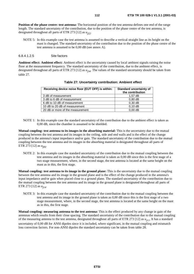
ETSI
ETSI TR 100 028-1 V1.3.1 (2001-03)112
Position of the phase centre: test antenna: The horizontal position of the test antenna defines one end of the rangelength. The standard uncertainty of the contribution, due to the position of the phase centre of the test antenna, isdesignated throughout all parts of ETR 273 [12] as uj22.
NOTE 5: In this example case the test antenna is assumed to describe a vertical straight line as its height on themast is changed. The standard uncertainty of the contribution due to the position of the phase centre of thetest antenna is assumed to be 0,00 dB (see annex A).
6.8.4.1.2.5 Site factors
Ambient effect: Ambient effect: Ambient effect is the uncertainty caused by local ambient signals raising the noisefloor at the measurement frequency. The standard uncertainty of the contribution, due to the ambient effect, isdesignated throughout all parts of ETR 273 [12] as uj34. The values of the standard uncertainty should be taken fromtable 27.
Table 27: Uncertainty contribution: Ambient effect
Receiving device noise floor (EUT OFF) is within: Standard uncertainty ofthe contribution
3 dB of measurement 1,57 dB3 dB to 6 dB of measurement 0,80 dB6 dB to 10 dB of measurement 0,30 dB10 dB to 20 dB of measurement 0,10 dB20 dB or more of the measurement 0,00 dB
NOTE 1: In this example case the standard uncertainty of the contribution due to the ambient effect is taken as0,00 dB, since the chamber is assumed to be shielded.
Mutual coupling: test antenna to its images in the absorbing material: This is the uncertainty due to the mutualcoupling between the test antenna and its images in the ceiling, side and end walls and is the effect of the changeproduced in the antenna's input impedance and/or gain. The standard uncertainty of the contribution due to the mutualcoupling between the test antenna and its images in the absorbing material is designated throughout all parts ofETR 273 [12] as uj06.
NOTE 2: In this example case the standard uncertainty of the contribution due to the mutual coupling between thetest antenna and its images in the absorbing material is taken as 0,00 dB since this is the first stage of atwo stage measurement, where, in the second stage, the test antenna is located at the same height on themast as in this, the first stage.
Mutual coupling: test antenna to its image in the ground plane: This is the uncertainty due to the mutual couplingbetween the test antenna and its image in the ground plane and is the effect of the change produced in the antenna'sinput impedance and/or gain when placed close to a ground plane. The standard uncertainty of the contribution due tothe mutual coupling between the test antenna and its image in the ground plane is designated throughout all parts ofETR 273 [12] as uj14.
NOTE 3: In this example case the standard uncertainty of the contribution due to the mutual coupling between thetest antenna and its image in the ground plane is taken as 0,00 dB since this is the first stage of a twostage measurement, where, in the second stage, the test antenna is located at the same height on the mastas in this, the first stage.
Mutual coupling: measuring antenna to the test antenna: This is the effect produced by any change in gain of theantennas which results from their close spacing. The standard uncertainty of the contribution due to the mutual couplingof the measuring antenna to the test antenna, designated throughout all parts of ETR 273 [12] as uj11, It has a standard
uncertainty of 0,00 dB for ANSI dipoles since it is included, where significant, in the mutual coupling and mismatchloss correction factors. For non-ANSI dipoles the standard uncertainty can be taken from table 28.

ETSI
ETSI TR 100 028-1 V1.3.1 (2001-03)113
Table 28: Uncertainty contribution of the mutual coupling between the measuring and test antenna
Frequency Standard uncertaintyof the contribution
(3 m range)
Standard uncertaintyof the contribution
(10 m range)30 MHz ≤ frequency < 80 MHz 1,73 dB 0,60 dB80 MHz ≤ frequency < 180 MHz 0,6 dB 0,00 dBfrequency ≥ 180 MHz 0,00 dB 0,00 dB
NOTE 4: In this example case the standard uncertainty of the contribution due to mutual coupling between themeasuring and test antennas is taken as 0,00 dB as we are using ANSI dipoles.
Mutual coupling: interpolation of mutual coupling and mismatch loss correction factors, only for ANSI dipoles:The standard uncertainty of the contribution, due to the interpolation of mutual coupling and mismatch loss correctionfactors, is designated throughout all parts of ETR 273 [12] as uj12. It has, for spot frequencies given in table A.20, avalue of 0,00 dB. However, for all other frequencies, the standard uncertainty should be obtained from table 29.
Table 29: Uncertainty contribution of the interpolation of mutual couplingand mismatch loss correction factors
Frequency (MHz) Standard uncertainty ofthe contribution
for a spot frequency given in the table 0,00 dB30 MHz ≤ frequency < 80 MHz 0,58 dB80 MHz ≤ frequency < 180 MHz 0,17 dBfrequency ≥ 180 MHz 0,00 dB
NOTE 5: In this example case the standard uncertainty of the contribution, due to the interpolation of mutualcoupling and mismatch loss correction factors, is taken as 0,00 dB as the frequency is above 180 MHz.
Range length: This contribution is associated with the curvature of the phase front from the measuring antenna to thetest antenna. The standard uncertainty of the contribution, due to range length, is designated throughout all parts ofETR 273 [12] as uj16. The standard uncertainty is 0,00 dB if ANSI dipoles are used. For other types of antenna thestandard uncertainty of the contribution should be obtained from table 30.
Table 30: Uncertainty contribution of the range length (verification)
Range length (i.e. the horizontal distancebetween phase centres)
Standard uncertainty of thecontribution
(d1+d2)2/4λ ≤ range length < (d1+d2)
2/2λ 1,26 dB(d1+d2)
2/2λ ≤ range length < (d1+d2)2/λ 0,30 dB
(d1+d2)2/λ ≤ range length < 2(d1+d2)
2/λ 0,10 dBrange length ≥ 2(d1+d2)
2/λ 0,00 dB
NOTE 6: In table 30, d1 and d2 are the maximum dimensions of the antennas.
NOTE 7: In this example case the standard uncertainty of the contribution, due to the range length, is taken as 0,00.
Reflectivity of absorbing material: measuring antenna to the test antenna: This uncertainty is the residual effect ofthe reflections in the absorbing materials which result from the measuring antenna and EUT having different elevationpatterns. The standard uncertainty of the contribution due to the reflectivity of absorbing material between themeasuring and test antenna is designated throughout all parts of ETR 273 [12] as uj02.
NOTE 8: In this example case the standard uncertainty of the contribution due to the reflectivity of absorbingmaterial between the measuring and test antenna is taken as 0,00 dB since a reference is set.

ETSI
ETSI TR 100 028-1 V1.3.1 (2001-03)114
Mutual coupling: measuring antenna to its images in the absorbing material: This uncertainty is the effect of thechange produced in the antenna's input impedance and/or gain. The standard uncertainty of the contribution, due to themutual coupling between the measuring antenna and its images in the absorbing material, is designated throughout allparts of ETR 273 [12] as uj06.
NOTE 9: In this example case the standard uncertainty of the contribution due to the mutual coupling between themeasuring antenna and its images in the absorbing material is taken as 0,5 dB.
Mutual coupling: measuring antenna to its image in the ground plane: This uncertainty is the effect of the changeproduced in the antenna's input impedance and/or gain. The standard uncertainty of the contribution, due to the mutualcoupling of the measuring antenna to its image in the ground plane, is designated throughout all parts of ETR 273 [12]as uj14. Its value can be obtained from table 31.
Table 31: Uncertainty contribution of the mutual coupling between the measuring antennaand its image in the ground plane
Spacing between the antennaand the ground plane
Standard uncertaintyof the contribution
For a vertically polarised antennaspacing ≤ 1,25 λ 0,15 dBspacing > 1,25 λ 0,06 dB
For a horizontally polarized antennaspacing < λ/2 1,15 dB
λ/2 ≤ spacing < 3λ/2 0,58 dB3λ/2 ≤ spacing < 3λ 0,29 dB
spacing ≥ 3λ 0,15 dB
NOTE 10:In this example case the standard uncertainty of the contribution due to the mutual coupling of themeasuring antenna to it's image in the ground plane is taken as 0,15 dB since we are assuming verticalpolarization and a spacing of < 1,25 λ.
6.8.4.1.2.6 Measuring antenna
Antenna: antenna factor of the measuring antenna: Uncertainty is introduced as a result of the inaccurate knowledgeof the antenna factor of the measuring antenna. The antenna factor of the measuring antenna is only involved in thesecond stage of the test and therefore does not act as a systematic offset. The standard uncertainty of the contribution,due to the antenna factor of the measuring antenna, is designated throughout all parts of ETR 273 [12] as uj44. For
ANSI dipoles the value should be obtained from table 32.
Table 32: Uncertainty contribution of the antenna factor of the measuring antenna.
Frequency Standard uncertainty of thecontribution
30 MHz ≤ frequency < 80 MHz 1,73 dB80 MHz ≤ frequency < 180 MHz 0,60 dBfrequency ≥ 180 MHz 0,30 dB
NOTE 1: For other antenna types the figures should be taken from manufacturers data sheets. If a figure is notgiven the standard uncertainty is 1,0 dB.
NOTE 2: In this example case the standard uncertainty of the contribution due to the antenna factor uncertainty ofthe receiving antenna is 0,30 dB since ANSI dipoles have been used and the frequency is above180 MHz.
Antenna: tuning of the measuring antenna Uncertainty is introduced as a result of the inaccurate tuning of themeasuring antenna. The standard uncertainty of the contribution due to the tuning of the measuring antenna isdesignated in the present document by uj46.
NOTE 3: In this example case the standard uncertainty of the contribution due to the tuning of the measuringantenna is taken to be 0,06 dB (see annex A) since the tuning of the measuring antenna is only involved inthis stage of the test and therefore does not act as a systematic offset.
ETSI
ETSI TR 100 028-1 V1.3.1 (2001-03)115
Position of the phase centre: measuring antenna: Uncertainty is introduced as a result of the inaccurate positioningof the phase centre of the measuring antenna, since it affects the range length i.e. the horizontal distance between itselfand the test antenna. The standard uncertainty of the contribution, due to the position of the phase centre of themeasuring antenna, is designated throughout all parts of ETR 273 [12] as uj22.
NOTE 4: In this example case the standard uncertainty of the contribution due to the position of the phase centre ofthe receiving antenna has been calculated from ± (the offset)/(range length) x 100 %). The positioninguncertainty is ±0,01 m and therefore the worst case uncertainty = 0,01/3,0 = 0,333 %. As the offset can beanywhere between these limits, the uncertainty is taken to be rectangularly distributed (see ETR 273 [12],part 1, subpart 1, clause 5.1.2) and the standard uncertainty is calculated as 0,192 %. This is transformedto the logarithmic form (ETR 028 [15], part 2, annex E), to be 0,02 dB.
6.8.4.1.2.7 Measuring antenna attenuator
Insertion loss: measuring antenna attenuator: The attenuator has an insertion loss as well as an uncertaintyassociated with the measurement of its magnitude. The value of insertion loss and its uncertainty remain valid providedthe attenuator is not used outside the manufacturer's specification. At any given frequency the insertion loss is takenfrom the manufacturer's data sheet since it does not cancel as a systematic offset (it only appears in one stage of thetest). The standard uncertainty of the contribution, due to the insertion loss uncertainty of the measuring antennaattenuator, is designated throughout all parts of ETR 273 [12] as uj40.
NOTE: In this example case the uncertainty of the contribution, due to the insertion loss uncertainty of themeasuring antenna attenuator, is taken from the manufacturer's data sheet as ±0,3 dB as nothing is saidabout the distribution, a rectangular distribution (see ETR 273 [12], part 1, subpart 1, clause 5.1.2) in logsis assumed and the standard uncertainty is calculated as 0,17 dB.
6.8.4.1.2.8 Measuring antenna cable
Insertion loss: measuring antenna cable: The measuring antenna cable has an insertion loss as well as an uncertaintyassociated with the measurement of its magnitude. The value of insertion loss and its uncertainty remain valid providedthe cable is not used outside the manufacturer's specification. At any given frequency the insertion loss acts as asystematic offset and contributes equally to both stages of the measurement. The standard uncertainty of thecontribution due to the insertion loss uncertainty of the measuring antenna cable, is designated throughout all parts ofETR 273 [12] as uj41.
NOTE 1: In this example case the uncertainty of the contribution due to the insertion loss uncertainty of themeasuring antenna cable is taken from the manufacturer's data sheet as ±0,5 dB. As nothing is said aboutthe distribution, a rectangular distribution (see ETR 273 [12], part 1, subpart 1, clause 5.1.2) in logs isassumed and the standard uncertainty is calculated as 0,29 dB.
Cable factor: measuring antenna cable: Cable factor is defined as the total effect of the antenna cable's influence onthe measuring system including its interaction with the site. It consists of the leakage caused by cable screeninginefficiency, parasitic effects (acting as a director or reflector) and introducing an unbalanced, common mode currentinto the dipole balun. In a radiated measurement the standard uncertainty of the cable factor associated with themeasuring antenna cable is 0,5 dB provided the precautions detailed in the method have been observed i.e. routing anddressing the cables with ferrites. If no prevention has been attempted the standard uncertainty is 4,0 dB (justification forthese values is given in ETR 273 [12], part 1, subpart 2, annex E). The standard uncertainty of the contribution, due tothe cable factor of the measuring antenna cable, is designated throughout all parts of ETR 273 [12] as uj19.
NOTE 2: In the example case the standard uncertainty of the contribution due to the cable factor of the measuringantenna cable is taken as 0,50 dB since the precautions detailed in the methods are assumed to have beenobserved.
ETSI
ETSI TR 100 028-1 V1.3.1 (2001-03)116
6.8.4.1.2.9 Receiving device
The receiving device is only used in the first stage of this test. Therefore, the absolute level uncertainty contributes fullyto this stage although the linearity does not.
Receiving device: absolute level: This uncertainty only contributes during the first stage of the measurement. Thestandard uncertainty of the contribution due to the receiving device absolute level uncertainty is designated throughoutall parts of ETR 273 [12] as uj47. Its value can be derived from manufacturers data.
NOTE 1: In this example case the uncertainty of the contribution due to the receiving device absolute leveluncertainty) is obtained from the manufacturers data as ±1 dB with a rectangular distribution (seeETR 273 [12], part 1, subpart 1, clause 5.1.2) in logs. The standard uncertainty of the contribution due tothe receiving device absolute level uncertainty is calculated as 0,58 dB.
Receiving device: linearity: In any test in which the contribution of the absolute level uncertainty of the receivingdevice contributes to the combined standard uncertainty of the test i.e. it does not cancel due to the methodology, thecontribution from the receiving device linearity is considered to have been included in uj47. Conversely, for any test in
which the absolute level uncertainty of the receiving device does not contribute to the combined standard uncertaintythe linearity of the receiving device should be included. The standard uncertainty of the contribution due to thereceiving device linearity is designated throughout all parts of ETR 273 [12] as uj48.
NOTE 2: In this example case the standard uncertainty of the contribution due to the receiving device linearity istaken as 0,00 dB.
6.8.4.1.3 Contribution from the random component
Random uncertainty: The magnitude can be assessed from multiple measurements of the Transform Factor. Thestandard uncertainty of the contribution due to the random uncertainty is designated throughout all parts ofETR 273 [12] as ui01.
The Transform Factor measurement was repeated 10 times. The following results were obtained in dBµV (beforecorrecting for cabling and attenuator network insertion loss):
- 65,4; 63,4; 66,0; 65,3; 63,0; 64,9; 65,2; 66,8; 65,5; 63,7.
Converting to linear terms:
- 1,862 × 10-3; 1,479 × 10-3; 1,995 × 10-3; 1,841 × 10-3; 1,413 × 10-3; 1,758 × 10-3; 1,820 × 10-3; 2,188 × 10-3;1,884 × 10-3; 1,531 × 10-3;
The two sums X and Y are calculated:
- X = the sum of the measured values = 17,77 × 10⁻³;
- Y = the sum of the squares of the measured values = 32,10 × 10⁻⁶ V2.
( )=
−
×−×=
−
−=
−−
11010
1077,171010,32
1
236
2
nn
XY
uc random 238,3 ×10⁻⁶ (formula 5.6)
As the result is obtained as the mean value of 10 measurements and the standard uncertainty of the random uncertaintyis:
dB,1715,11
100
10777,1
103,2383
6=×
×
×=−
−
j randomu
NOTE: In this example case the standard uncertainty of the contribution due to the random uncertainty is 1,17 dB.

ETSI
ETSI TR 100 028-1 V1.3.1 (2001-03)117
6.8.4.1.4 Summary table of contributory components
All the uncertainties for this part of the procedure are listed in table 33.
Table 33: Contributions from the transfer factor measurement
uj or i Description of uncertainty contributions dBuj36 mismatch: transmitting part 0,00uj37 mismatch: receiving part 0,11uj38 signal generator: absolute output level 0,58uj39 signal generator: output level stability 0,00uj41 insertion loss: test antenna cable 0,00uj19 cable factor: test antenna cable 0,00uj40 insertion loss: test antenna attenuator 0,00uj18 correction: measurement distance 0,00uj17 correction: off boresight angle in elevation plane , 0,00uj45 antenna: gain of the test antenna 0,00uj46 antenna: tuning of the test antenna 0,00uj22 position of the phase centre: test antenna 0,00uj34 ambient effect 0,00uj06 mutual coupling: test antenna to its images in the absorbing material 0,00uj14 mutual coupling: test antenna to its image in the ground plane 0,00uj11 mutual coupling: measuring antenna to the test antenna 0,00uj12 mutual coupling: interpolation of mutual coupling and mismatch loss correction factors 0,00uj16 range length 0,00uj02 reflectivity of absorber material: measuring antenna to the test antenna 0,00uj06 mutual coupling: measuring antenna to its images in the absorbing material 0,50uj14 mutual coupling: measuring antenna to its image in the ground plane 0,15uj44 antenna: antenna factor of the measuring antenna 0,30uj46 antenna: tuning of the measuring antenna 0,06uj22 position of the phase centre: measuring antenna 0,02uj40 insertion loss: measuring antenna attenuator 0,17uj41 insertion loss: measuring antenna cable 0,29uj19 cable factor: measuring antenna cable 0,50uj47 receiving device: absolute level 0,58uj48 receiving device: linearity 0,00ui01 random uncertainty 1,17
The standard uncertainties from table 33 should be combined by RSS in accordance with ETR 273 [12], part 1,subpart 1, clause 5. This gives the combined standard uncertainty (uc Transform Factor) for the Transform Factormeasurement in dB.
The value of uc Transform Factor is calculated as 1,67 dB.
6.8.4.2 Uncertainty contributions: Stage 2: EUT measurement
The second stage of the measurement (EUT sensitivity measurement) is to determine the minimum signal generatoroutput level which produces the required response from the EUT and converting the output level of the signal generator,to a field strength using the Transform Factor derived in stage one. The test equipment set-up is shown in figure 31. Thecomponents shown shaded are common to both stages of the test.

ETSI
ETSI TR 100 028-1 V1.3.1 (2001-03)118
Testantennacable 2
ferrite beads
Test antenna
Signalgenerator
Attenuator 210 dB
EUT
Ground plane
Figure 31: EUT measurement
Whereas figure 31 shows, schematically, the test equipment for the EUT sensitivity measurement, figure 32 an analysisdiagram, provides a detailed picture of the individual uncertainty components (each of which contributes its ownuncertainty) for this stage in the measurement. As stated above, the shaded areas represent components common to bothstages of the test method.
6.8.4.2.1 Contributions from the mismatch components
Mismatch: transmitting part: Only the transmitting part of the test equipment set-up is involved in this stage of thetest. The standard uncertainty of the contribution due to mismatch is 0,00 dB since, as stated in clause 6.8.4.1.1 thetransmitting part is common to both stages of the test.
Signal
Test antennaSite factors
Cablefactor
Testantennacable 2
Cableloss
Attenuator 210 dB
Equipmentunder test
generator
Antenna toEUT
coupling
Mutualimage
coupling
Antennagain
+
+
SINADmeterEUT
Siteeffects
Reflectedpath loss
Directpath loss
Signalgenerator
Mismatch
Mismatch
Mismatch
+
+
Figure 32: Reference for the measurement on the equipment (sensitivity)
ETSI
ETSI TR 100 028-1 V1.3.1 (2001-03)119
The mismatch uncertainty between the signal generator and the test antenna contributes equally to both stages of the testand therefore it does not contribute to the combined standard uncertainty and is not calculated. The standard uncertaintyof the contribution due to mismatch in the transmitting part is designated throughout all parts of ETR 273 [12] as uj35.
NOTE: In this example case the standard uncertainty of the contribution due to mismatch in the transmitting partis taken as 0,00 dB, since the uncertainty is systematic i.e. it produces the same offset in both stages.
6.8.4.2.2 Contributions from the individual components
6.8.4.2.2.1 Signal generator
Signal generator: absolute output level: There is not necessarily any similarity between the output levels from thesignal generator in the two stages of this test. As a result it contributes to both stages. The standard uncertainty of thecontribution, due to the signal generator absolute output level, is designated throughout all parts of ETR 273 [12] asuj38. Its value can be derived from manufacturer's data sheet.
NOTE 1: In this example case the uncertainty of the contribution due to the signal generator absolute output leveluncertainty is taken from the manufacturers data sheet as ±1,0 dB. As nothing is said about thedistribution of this uncertainty, a rectangular distribution (see ETR 273 [12], part 1, subpart 1,clause 5.1.2) in logs is assumed, and the standard uncertainty is calculated as 0,58 dB.
Signal generator: output level stability: In any test in which the contribution of the absolute level uncertainty of thesignal generator contributes to the combined standard uncertainty of the test i.e. it does not cancel due to themethodology, the contribution from the output level stability is considered to have been included in the signal generatorabsolute output level, uj38. Conversely, for any level in which the absolute level uncertainty of the signal generator does
not contribute to the combined standard uncertainty, the output level stability of the signal generator should be included.The standard uncertainty of the contribution due to the signal generator output level stability is designated throughoutall parts of ETR 273 [12] as uj39. Its value can be derived from manufacturers' data sheet.
NOTE 2: In this example case the standard uncertainty of the contribution due to the signal generator output levelstability is taken as 0,00 dB as it is covered by the absolute level uncertainty.
6.8.4.2.2.2 Test antenna cable
Insertion loss: test antenna cable: The test antenna cable has an insertion loss as well as an uncertainty associatedwith the measurement of its magnitude. The value of insertion loss and its uncertainty remain valid provided the cable isnot used outside the manufacturer's specification. At any given frequency the insertion loss acts as a systematic offsetand contributes equally to both stages of the measurement. The standard uncertainty of the contribution due to theinsertion loss uncertainty of the test antenna cable is designated throughout all parts of ETR 273 [12] as uj41.
NOTE 1: In this example case the standard uncertainty of the contribution due to the insertion loss uncertainty ofthe test antenna cable is taken as 0,00 dB since the uncertainty is systematic i.e. it produces the sameoffset in both stages.
Cable factor: test antenna cable: Cable factor is defined as the total effect of the antenna cable's influence on themeasuring system including it's interaction with the site. It consists of the leakage caused by cable screeninginefficiency, parasitic effects (acting as a director or reflector) on the test antenna and introducing an unbalanced,common mode current into the dipole balun. In a radiated measurement the standard uncertainty of the cable factor,associated with each cable, is 0,5 dB provided that the precautions detailed in the methods have been observed.i.e. routing and dressing of cables with ferrites. If no prevention has been attempted the standard uncertainty is 4,0 dB(justification for these values is given in ETR 273 [12], part 1, subpart 2, annex E). The standard uncertainty of thecontribution due to the cable factor of the test antenna cable is designated throughout all parts of ETR 273 [12] as uj19.
NOTE 2: In this example case the standard uncertainty of the contribution due to the cable factor of the test antennacable is taken as 0,00 dB since in this measurement, the cable position, once set in stage 1, is notsubsequently changed during the test.
ETSI
ETSI TR 100 028-1 V1.3.1 (2001-03)120
6.8.4.2.2.3 Test antenna attenuator
Insertion loss: test antenna attenuator: The test antenna attenuator has an insertion loss as well as an uncertaintyassociated with the measurement of its magnitude. The value of insertion loss and its uncertainty remain valid providedthe attenuator is not used outside the manufacturer's specification. At any given frequency the insertion loss acts as asystematic offset and contributes equally to both stages of the measurement. The standard uncertainty of thecontribution due to the insertion loss of the test antenna attenuator is designated throughout all parts of ETR 273 [12] asuj40.
NOTE: In this example case the standard uncertainty of the contribution, due to the insertion loss uncertainty ofthe test antenna attenuator, is taken as 0,00 dB since the uncertainty is systematic i.e. it produces the sameoffset in both stages.
6.8.4.2.2.4 Test antenna
Correction: measurement distance: For those tests in which the test antenna on the mast peaks at different heights inthe two stages, a correction for measurement distance must be made to account for the different measurement distances.In this test, once the position of the test antenna is set in stage one no further adjustment to its position is subsequentlymade during the test. The standard uncertainty of the contribution due to the correction for measurement distance isdesignated throughout all parts of ETR 273 [12] as uj18.
NOTE 1: In this example case the standard uncertainty of the contribution due to the correction for measurementdistance is taken as 0,00 dB.
Correction: off boresight angle in elevation plane: For those tests in which the test antenna on the mast peaks atdifferent heights in the two stages, a correction must be made to account for the different angles subtended by theEUT/substitution antenna. In this test, once the position of the test antenna is set in stage one no further adjustment to itsposition is subsequently made during the test. The standard uncertainty of the contribution due to the correction for offboresight angle in elevation plane is designated throughout all parts of ETR 273 [12] as uj17.
NOTE 2: In this example case the standard uncertainty of the contribution due to the correction for off boresightangle in elevation plane is taken as 0,00 dB since the uncertainty is assumed to be systematic i.e. it isassumed constant and common to both stages of the measurement.
Antenna: gain of the test antenna: The gain of the test antenna acts as a systematic offset since it is present in bothstages of the test. The standard uncertainty of the contribution due to the gain of the test antenna is designatedthroughout all parts of ETR 273 [12] as uj45.
NOTE 3: In this example case the standard uncertainty of the contribution due to the gain of the test antenna istaken as 0,00 dB since the uncertainty is assumed to be systematic i.e. it is assumed constant and commonto both stages of the measurement.
Antenna: tuning of the test antenna: This uncertainty is introduced as a result of inaccurate tuning of the test antenna.The standard uncertainty of the contribution due to the tuning of the test antenna is designated throughout all parts ofETR 273 [12] as uj46.
NOTE 4: In this example case the standard uncertainty of the contribution due to the tuning of the test antenna istaken as 0,00 dB since the uncertainty is assumed to be systematic i.e. it is assumed constant and commonto both stages of the measurement (provided that once set in stage one of the test it is not subsequentlyre-tuned).
Position of the phase centre: test antenna: The horizontal position of the test antenna defines one end of the rangelength. Since the test antenna position on the mast is not changed after being set in this stage the standard uncertainty ofthe contribution due to the position of the phase centre of the test antenna is designated throughout all parts ofETR 273 [12] as uj22.
NOTE 5: In this example case the standard uncertainty of the contribution due to the position of the phase centre ofthe test antenna is taken as 0,00 dB since the uncertainty is assumed to be systematic i.e. it is assumedconstant and common to both stages of the measurement.

ETSI
ETSI TR 100 028-1 V1.3.1 (2001-03)121
6.8.4.2.2.5 Site factors
Ambient effect: Ambient effect is the uncertainty caused by local ambient signals raising the noise floor at themeasurement frequency. The standard uncertainty of the contribution due to the ambient effect is designated throughoutall parts of ETR 273 [12] as uj34. The values of the standard uncertainties for this part of the test should be the same as
for stage 1.
NOTE 1: In this example case the standard uncertainty of the contribution due to the ambient effect is taken as0,00 dB as this was the value in stage 1.
Range length: This contribution is associated with the curvature of the phase front from the EUT to the test antenna.The standard uncertainty of the contribution, due to range length, is designated throughout all parts of ETR 273 [12] asuj16. The standard uncertainty is 0,00 dB if ANSI dipoles are used. For other types of antenna the standard uncertaintyof the contribution should be obtained from table 34.
Table 34: Uncertainty contribution of the range length (verification)
Range length (i.e. the horizontal distancebetween phase centres)
Standard uncertainty of thecontribution
(d1+d2)2/4λ ≤ range length < (d1+d2)
2/2λ 1,26 dB(d1+d2)
2/2λ ≤ range length < (d1+d2)2/λ 0,30 dB
(d1+d2)2/λ ≤ range length < 2(d1+d2)
2/λ 0,10 dBrange length ≥ 2(d1+d2)
2/λ 0,00 dB
NOTE 2: In table 34, d1 and d2 are the maximum dimensions of the antennas.
NOTE 3: In this example case the standard uncertainty of the contribution due to the range length is taken as0,00 dB since the range length is ≥ 2 (d1+d2)2/λ.
Mutual coupling: amplitude effect of the test antenna on the EUT: This uncertainty results from the interactionbetween the EUT and the test antenna when placed close together. The standard uncertainty of the contribution due tothe amplitude effect of the mutual coupling between the test antenna and the EUT, is designated throughout all parts ofETR 273 [12] as uj08. The standard uncertainty should be taken from table 35.
Table 35: Uncertainty contribution: Mutual coupling: amplitude effect of the test antenna on the EUT
Range length Standard uncertainty of thecontribution
0,62√((d1+d2)3/λ)≤ range length < 2(d1+d2)
2/λ 0,50 dBrange length ≥ 2(d1+d2)
2/λ 0,00 dB
NOTE 4: In this example case the standard uncertainty of the contribution due to the amplitude effect of the mutualcoupling between the test antenna and the EUT is 0,00 dB since the distance is ≥ 2 (d1+d2)2/λ.
Mutual coupling: EUT to its images in the absorbing material: This uncertainty is dependant on the quality of theabsorbing material and the effect imaging of the EUT in the ceiling, side and end walls has on the input impedanceand/or gain of the integral antenna. The standard uncertainty of the contribution, due to the mutual coupling of the EUTto its images in the absorbing material, is designated throughout all parts of ETR 273 [12] as uj04.
NOTE 5: In this example case the standard uncertainty of the contribution due to the mutual coupling amplitudeeffect of the absorbing material on the EUT is assumed to be 0,5 dB (see annex A).
Mutual coupling: EUT to its image in the ground plane: This uncertainty results from the change in the EUTspurious emission level as a result of being placed close to the ground plane. The standard uncertainty of thecontribution, due to the mutual coupling of the EUT to its image in the ground plane, is designated throughout all partsof ETR 273 [12] as uj13. Its value can be obtained from table 36.

ETSI
ETSI TR 100 028-1 V1.3.1 (2001-03)122
Table 36: Uncertainty contribution of the mutual couplingbetween the EUT to its image in the ground plane
Spacing between the EUTand the ground plane
Standard uncertaintyof the contribution
For a vertically polarized EUTspacing ≤ 1,25 λ 0,15 dBspacing > 1,25 λ 0,06 dB
For a horizontally polarized EUTspacing < λ/2 1,15 dB
λ/2 ≤ spacing < 3λ/2 0,58 dB3λ/2 ≤ spacing < 3λ 0,29 dB
spacing ≥ 3λ 0,15 dB
NOTE 6: In this example case the standard uncertainty of the contribution, due to the mutual coupling of the EUTto its image in the ground plane, (assuming the polarization is vertical and the spacing above the groundplane is < 1,25 λ at the test frequency) is taken as 0,15 dB.
Reflectivity of absorbing material: EUT to the test antenna. This uncertainty is associated with the magnitudes ofthe reflections occurring from the side walls, end walls and ceiling. These magnitudes are a function of the quality ofthe absorber at the frequency of test. The standard uncertainty of the contribution, due to the reflectivity of theabsorbing material between the EUT and the test antenna, is designated throughout all parts of ETR 273 [12] as uj01.
The relevant value for this contribution should be taken from table 37.
Table 37: Uncertainty contribution of the reflectivityof absorbing material between the EUT and test antenna
Reflectivity of theabsorbing material
Standard uncertainty of thecontribution
reflectivity < 10 dB 4,76 dB10 ≤ reflectivity < 15 dB 3,92 dB15 ≤ reflectivity < 20 dB 2,56 dB20 ≤ reflectivity < 30 dB 1,24 dBreflectivity ≥ 30 dB 0,74 dB
NOTE 7: In this example case the standard uncertainty of the contribution due to the reflectivity of the absorbingmaterial between the EUT and the test antenna is taken as 1,24 dB.
Mutual coupling: test antenna to its images in the absorbing material: This is the uncertainty due to the mutualcoupling between the test antenna and its images in the ceiling, side and end walls and is the effect of the changeproduced in the antenna's input impedance and/or gain. The standard uncertainty of the contribution, due to the mutualcoupling between the test antenna and its images in the absorbing material, is designated throughout all parts ofETR 273 [12] as uj06.
NOTE 8: In this example case the standard uncertainty of the contribution due to the mutual coupling between thetest antenna and its images in the absorbing material is taken as 0,00 dB since in this, the second stage ofthe measurement, the uncertainty will only contribute if the test antenna is located at a different height tothe first stage which is not allowed by the methodology hence the uncertainty is assumed to be systematici.e. it is assumed constant and common to both stages of the measurement.
Mutual coupling: test antenna to its image in the ground plane: This is the uncertainty due to the mutual couplingbetween the test antenna and its image in the ground plane and is the effect of the change produced in the antenna'sinput impedance and/or gain when placed close to a ground plane. The standard uncertainty of the contribution, due tothe mutual coupling of the test antenna to its image in the ground plane, is designated throughout all parts ofETR 273 [12] as uj14.
NOTE 9: In this example case the standard uncertainty of the contribution due to the mutual coupling of the testantenna to its image in the ground plane is taken as 0,00 dB since in this, the second stage of themeasurement, the uncertainty will only contribute if the test antenna is located at a different height to thefirst stage which is not allowed by the methodology hence the uncertainty is assumed to be systematici.e. it is assumed constant and common to both stages of the measurement.
ETSI
ETSI TR 100 028-1 V1.3.1 (2001-03)123
6.8.4.2.2.6 EUT
EUT: mutual coupling to the power leads: This is the uncertainty associated with the influence (reflections, parasiticeffects, etc.) of the power leads on the EUT. The standard uncertainty associated with this effect is 0,5 dB provided thatthe precautions detailed in the methods have been observed. i.e. routing and dressing of cables with ferrites. If noprevention has been attempted the standard uncertainty is 2,0 dB. The standard uncertainty of the contribution, due tothe mutual coupling of the EUT to the power leads, is designated throughout all parts of ETR 273 [12] as uj54.
NOTE 1: In this example case the standard uncertainty of the contribution due to the mutual coupling of the EUT tothe power leads is taken as 0,5 dB since the precautions detailed in the methods have been observed.
Position of the phase centre: within the EUT volume: This contribution is associated with the uncertainty with whichthe actual radiating point within the equipment volume is known. If this point is known exactly the contribution is0,00 dB. The standard uncertainty of the contribution due to the position of the phase centre within the EUT volume isdesignated throughout all parts of ETR 273 [12] as uj20.
NOTE 2: In this example case the standard uncertainty of the contribution due to the position of the phase centrewithin the EUT volume has been calculated from (±(the maximum dimension of device)/(2 × rangelength) × 100 %). In this example the position is not known. Hence, the uncertainty of the position of thephase centre within the EUT of 0,15 m maximum dimension is 0,15/2 m = 0,075 m, and the worst caseuncertainty due to this offset is therefore (0,075/3,0) × 100 % = ±2,50 %. As the phase centre can beanywhere inside the EUT, the uncertainty is taken as rectangularly distributed and the standarduncertainty is calculated as 1,44 %. This is then transformed to the logarithmic form(1,44/11,5) = 0,12 dB (ETR 028 [15], part 2, annex E).
Positioning of the phase centre: within the EUT over the axis of rotation of the turntable: This contribution isassociated with the uncertainty with which the actual radiating point within the equipment is placed over the centre ofthe turntable. If the point is placed exactly, the contribution is 0,00 dB. The standard uncertainty of the contribution, dueto the positioning of the phase centre within the EUT over the axis of rotation of the turntable, is designated throughoutall parts of ETR 273 [12] as uj21.
NOTE 3: In this example case the standard uncertainty of the contribution due to the positioning of the EUT phasecentre over the axis of rotation of the turntable is calculated from (±(the estimated offset from the axis ofrotation)/(2 × range length) × 100 %). In this case, the uncertainty is taken as ±0,01 m, and the worst caseuncertainty is ±(0,01/3,0) × 100 = ±0,333 %. As the offset can be anywhere between the limits theuncertainty is rectangularly distributed and the standard uncertainty is calculated as 0,192 %. This is thentransformed to the logarithmic form (0,192/11,5) = 0,02 dB (ETR 028 [15], part 2, annex E).
EUT: degradation measurement: This contribution is a RF level uncertainty associated with the uncertainty ofmeasuring 20 dB SINAD, 10-2 bit stream or 80 % message acceptance ratio. The standard uncertainty of thecontribution, due to the EUT degradation measurement, is designated throughout all parts of ETR 273 [12] as uj52. Itsvalue can be obtained from ETR 028 [15].
NOTE 4: In this example case, the standard uncertainty of the contribution is obtained from ETR 028 [15] and itsvalue is 0,68 dB.
6.8.4.2.3 Contribution from the random component
Random uncertainty: The magnitude can be assessed from multiple measurements of the receiver sensitivity. Thestandard uncertainty of the contribution due to the random uncertainty is designated throughout all parts ofETR 273 [12] as ui01.
The receiver sensitivity measurement was repeated 10 times. The following results were obtained in dBµV (beforecorrecting for cabling and attenuator network insertion loss):
- 65,4; 63,4; 66,0; 65,3; 63,0; 64,9; 65,2; 66,8; 65,5; 63,7.
Converting to linear terms:
- 1,862 × 10-3; 1,479 × 10-3; 1,995 × 10-3; 1,841 × 10-3; 1,413 × 10-3; 1,758 × 10-3; 1,820 × 10-3; 2,188 × 10-3;1,884 × 10-3; 1,531 × 10-3.
ETSI
ETSI TR 100 028-1 V1.3.1 (2001-03)124
The two sums X and Y are calculated:
- X = the sum of the measured values = 17,77 × 10⁻³;
- Y = the sum of the squares of the measured values = 32,10 × 10⁻⁶ V2.
( )=
−
×−×=
−
−=
−−
11010
1077,171010,32
1
236
2
nn
XY
uc random 238,3 ×10⁻⁶ (formula 5.6)
As the result is obtained as the mean value of 10 measurements and the standard uncertainty of the random uncertaintyis:
dB1,175,11
100
10777,1
103,2383
6=×
×
×=−
−
j randomu
NOTE: In this example case the standard uncertainty of the contribution due to the random uncertainty is 1,17 dB.
6.8.4.2.4 Summary table of contributory components
All the uncertainty contributions for this part of the procedure are listed in table 38.
Table 38: Contributions from the EUT measurement
uj or i Description of uncertainty contributions dBuj36 mismatch: transmitting part 0,00uj38 signal generator: absolute output level 0,58uj39 signal generator: output level stability 0,00uj41 insertion loss: test antenna cable 0,00uj19 cable factor: test antenna cable 0,00uj40 insertion loss: test antenna attenuator 0,00uj17 correction: off boresight angle in elevation plane 0,00uj18 correction: measurement distance 0,00uj45 antenna: gain of the test antenna 0,00uj46 antenna: tuning of the test antenna 0,00uj22 position of the phase centre: test antenna 0,00uj34 ambient effect 0,00uj08 mutual coupling: amplitude effect of the test antenna on the EUT 0,00uj04 Mutual coupling: EUT to its images in the absorbing material 0,50uj13 mutual coupling: EUT to its image in the ground plane 0,15uj01 reflectivity of absorber material: EUT to the test antenna 1,24uj06 mutual coupling: test antenna to its images in the absorbing material 0,00uj14 mutual coupling: test antenna to its image in the ground plane 0,00uj55 EUT: mutual coupling to the power leads 0,50uj20 position of the phase centre: within the EUT volume 0,12uj22 positioning of the phase centre: within the EUT over the axis of rotation of the turntable 0,02uj16 range length 0,00uj52 EUT: degradation measurement 0,68ui01 random uncertainty 1,17
The standard uncertainties from table 38 should be combined by RSS in accordance with ETR 273 [12], part 1,subpart 1, clause 5. This gives the combined standard uncertainty (uc EUT measurement) for the NSA measurement in dB.
The value of uc EUT measurement is calculated as 2,06 dB.

ETSI
ETSI TR 100 028-1 V1.3.1 (2001-03)125
6.8.4.2.5 Expanded uncertainty for the receiver Sensitivity measurement
The combined standard uncertainty of the results of the verification procedure is the combination of the componentsoutlined in clauses 6.8.2.1.4 and 6.8.2.2.4. The components to be combined are uc Transform Factor and uc EUT measurement.
dB2,65=06,267,1 22 +=tmeasuremenySensitivitcu
The expanded uncertainty is ±1,96 x 2,65 dB = ±5,19 dB at a 95 % confidence level.
6.9 Examples of measurement uncertainty analysis (Stripline)
6.9.1 Introduction
This clause contains detailed worked examples of the calculation of expanded uncertainty of radiated tests in a Striplinetest facility.
The example tests given are limited to:
- a verification procedure;
- the measurement of a receiver parameter (Sensitivity).
Both of the example tests are assumed to have been carried out in the 2-plate open Stripline described in CENELECEuropean Standard EN 55020 [16].
NOTE 1: The values given to all of the uncertainty components in these examples are only to illustrate theuncertainty calculation. In practice, values should be derived by consulting annex A.
All radiated tests consist of two stages. For the verification procedure, the first stage is to set a reference level whilst thesecond stage involves the measurement of path loss/attenuation through the Stripline. For the measurement of thereceive sensitivity of an EUT, the first stage is to find the minimum (or average) signal generator output that producesthe required receiver response, whilst the second stage determines the field strength in the Stripline corresponding tothat generator output level.
Within any radiated test there are uncertainty components that are common to both stages of the test. By their differentnatures some of these common uncertainties will cancel (e.g. the uncertainty of the insertion loss of a cable common toboth parts), others will contribute once (e.g. the increase in the field strength caused by a large EUT) whilst others maycontribute twice (e.g. the level stability of a signal generator in receiver tests). In each of the following uncertaintyanalyses, uncertainty components common to both stages are shown as shaded areas in the accompanying schematicdiagrams.
As shown in the examples, all the individual uncertainty components for any test are combined in the manner describedin ETR 273 [12], part 1, subpart 1, clauses 4 and 5 in order to derive an expanded uncertainty figure for themeasurement. The values of the individual components are either provided in annex A or should be taken frommanufacturers' data sheets. Whenever they are obtained from data sheets, worst case figures given over a frequencyband should be used. For example, in the case of a signal generator whose absolute level accuracy is quoted as ±1 dBover 30 MHz to 300 MHz, ±2 dB over 300 MHz to 1 000 MHz the figure for the band containing the test frequencyshould be used. This approach should be adopted for all uncertainty components, taking the uncertainty figures over asbroad a band a possible. This is normally satisfactory when the variation with frequency is not large and provides asimple and flexible approach. The resulting expanded uncertainty figure is valid across a broad range of frequencies andmeasurement conditions and avoids the necessity of repeated calculation for minor frequency changes.
NOTE 2: Taking specific frequency values may result in a lower expanded uncertainty value, but this lower value isonly valid when that specific set of circumstances apply for which the value was derived.
6.9.2 Example 1: Verification procedure
The Stripline verification procedure involves two different measurement stages and it results in values for both theattenuation through the Stripline and its Transform Factor (i.e. the relationship between the input voltage to the Striplineand the resulting field strength between the plates).

ETSI
ETSI TR 100 028-1 V1.3.1 (2001-03)126
6.9.2.1 Uncertainty contributions: Stage 1: Direct attenuation measurement
The first stage of the verification procedure is the direct attenuation measurement. This is carried out with all the itemsof test equipment connected directly together via an "in line" adapter between the attenuators as shown in figure 33. Thecomponents shown shaded are common to both stages of the procedure.
"In line"adapter
Attenuator 210 dB
Receivingdevice
Attenuator 110 dB
Signalgenerator
cable 1 cable 2
ferrite beads ferrite beads
Figure 33: Stage 1: Direct attenuation measurement
Despite the commonality of most of the components to both stages of this procedure, the mismatch uncertaintycontribution for both stages has to be calculated and included in the uncertainty calculations. This is the result of loadconditions varying (i.e. the Stripline and monopole replaces the adapter in the second stage). Conversely, as a result ofthis commonality, the uncertainty contributions of some of the individual components will cancel.
Whereas figure 33 shows, schematically, the test equipment set-up for this stage of the verification procedure, ananalysis diagram of the individual components (each of which contributes its own uncertainty) for this stage of themeasurement is shown in figure 34. Again, as stated above, the shaded areas represent components common to bothstages of the verification procedure.
6.9.2.1.1 Contributions from the mismatch components
Mismatch: direct attenuation measurement: The value of the combined standard uncertainty of the contribution dueto the mismatch from the source to the receptor, i.e. between the signal generator and the receiving device, is calculatedfrom the approach described in annex G. All the individual contributions are U-distributed.
NOTE 1: In this example the signal generator output reflection coefficient used is the worst case magnitude overthe frequency band of interest, as is the case with the cable, adapter and attenuator VSWRs.
NOTE 2: The attenuation values of the cables and attenuators should be obtained from the manufacturers datasheet/calibration records at the specific frequency of the test, along with the associated uncertainties forthese values.
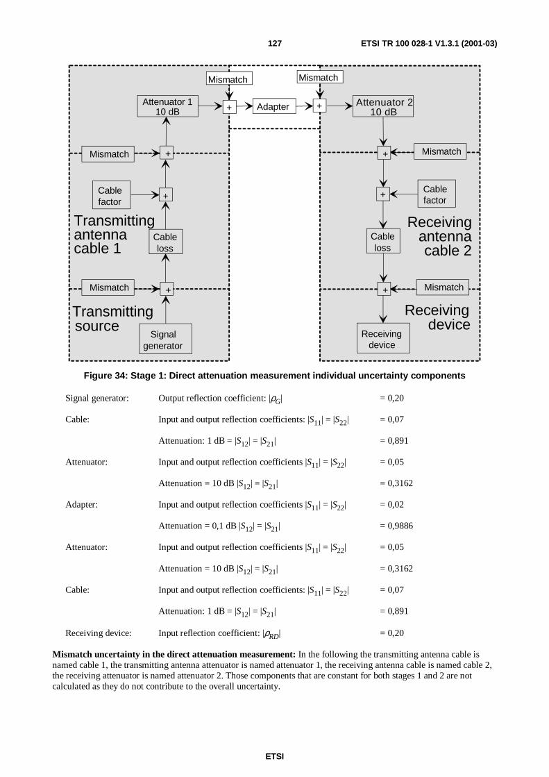
ETSI
ETSI TR 100 028-1 V1.3.1 (2001-03)127
Receivingdevice
Cablefactor
Cableloss
Receivingdevice
Signalgenerator
Cableloss
Cablefactor
Receivingantennacable 2
Transmittingantennacable 1
sourceTransmitting
Adapter
Mismatch
Attenuator 110 dB
Mismatch
++
+ + Attenuator 210 dB
Mismatch
Mismatch
Mismatch
Mismatch +
+
+
+
Figure 34: Stage 1: Direct attenuation measurement individual uncertainty components
Signal generator: Output reflection coefficient: |ρG| = 0,20
Cable: Input and output reflection coefficients: |S11| = |S22| = 0,07
Attenuation: 1 dB = |S12| = |S21| = 0,891
Attenuator: Input and output reflection coefficients |S11| = |S22| = 0,05
Attenuation = 10 dB |S12| = |S21| = 0,3162
Adapter: Input and output reflection coefficients |S11| = |S22| = 0,02
Attenuation = 0,1 dB |S12| = |S21| = 0,9886
Attenuator: Input and output reflection coefficients |S11| = |S22| = 0,05
Attenuation = 10 dB |S12| = |S21| = 0,3162
Cable: Input and output reflection coefficients: |S11| = |S22| = 0,07
Attenuation: 1 dB = |S12| = |S21| = 0,891
Receiving device: Input reflection coefficient: |ρRD| = 0,20
Mismatch uncertainty in the direct attenuation measurement: In the following the transmitting antenna cable isnamed cable 1, the transmitting antenna attenuator is named attenuator 1, the receiving antenna cable is named cable 2,the receiving attenuator is named attenuator 2. Those components that are constant for both stages 1 and 2 are notcalculated as they do not contribute to the overall uncertainty.

ETSI
ETSI TR 100 028-1 V1.3.1 (2001-03)128
Mismatch between:
- uj generator and cable 1: Constant for both stage 1 and 2. Hence this value does not contribute.
- uj cable 1 and attenuator 1: Constant for both stage 1 and 2. Hence this value does not contribute.
%0,071%2
10002,005,01: =××=adapterandattenuatormismatchju
%0,071%2
10005,002,01: =××=attenuatorandadaptermismatchju
- uj attenuator 2 and cable 2: Constant for both stage 1 and 2. Hence this value does not contribute.
- uj cable 2 and receiving device: Constant for both stage 1 and 2. Hence this value does not contribute.
- uj generator and attenuator 1: Constant for both stage 1 and 2. Hence this value does not contribute.
%0,035%2
100316,007,007,0 2
1: =×××=adapterandcablemismatchju
%0,173%2
100988,005,005,0 2
21: =×××=attenuatorandattenuatormismatchju
%0,010%2
100316,007,002,0 2
2: =×××=cableandadaptermismatchju
- uj attenuator 2 and receiving device: Constant for both stage 1 and 2. Hence this value does not contribute.
%0,022%2
100316,0891,002,02,0 22
: =××××=adapterandgeneratormismatchju
%0,024%2
100988,0316,005,007,0 22
21: =××××=attenuatorandcablemismatchju
%0,024%2
100316,0988,007,005,0 22
21: =××××=cableandattenuatormismatchju
%0,022%2
100891,0316,02,002,0 22
: =××××=devicereceivingandadaptermismatchju
%0,055%2
100988,0316,0891,005,02,0 222
2: =×××××=attenuatorandgeneratormismatchju
- uj mismatch: cable 1 and cable 2: Less than 0,01 % due to the two attenuators, therefore neglected.
%0,055%2
100891,0316,0988,02,005,0 222
1: =×××××=devicereceivingandattenuatormismatchju
- uj mismatch: generator and cable 2: Less than 0,01 % due to the two attenuators, therefore neglected.
- uj mismatch: cable 1 and receiving device: Less than 0,01 % due to the two attenuators, therefore neglected.
- uj mismatch: generator and receiving device: Less than 0,01 % due to the two attenuators, therefore neglected.

ETSI
ETSI TR 100 028-1 V1.3.1 (2001-03)129
The combined standard uncertainty of the mismatch is then calculated:
%0,306055,0055,0...071,0071,0 2222.: =++++=attdirectmismatchcu
Transforming to logarithmic form (ETR 028 [15], part 2, annex E): 0,306 %/11,5 = 0,026 dB.
The standard uncertainty of the contribution, due to the mismatch in the direct attenuation measurement, is designatedthroughout all parts of ETR 273 [12] as uj35. Its value in this example is 0,026 dB.
6.9.2.1.2 Contributions from individual components
6.9.2.1.2.1 Signal generator
Signal generator: absolute output level: In a verification procedure, the signal generator's absolute level uncertaintycontributes equally to both stages of the measurement. The standard uncertainty of the contribution due to the signalgenerator absolute output level uncertainty is designated throughout all parts of ETR 273 [12] as uj38.
NOTE 1: In this example case the standard uncertainty of the contribution due to the signal generator absoluteoutput level uncertainty is taken to be 0,00 dB since, once the level has been set in stage one of theprocedure, the level is not further adjusted. The uncertainty is therefore assumed to be systematic i.e. itproduces the same offset in both stages.
Signal generator: output level stability: In any test in which the contribution of the absolute level uncertainty of thesignal generator contributes to the combined standard uncertainty of the test i.e. it does not cancel due to themethodology, the contribution from the output level stability is considered to have been included in the signal generatorabsolute output level, uj38. Conversely, for any level in which the absolute level uncertainty of the signal generator doesnot contribute to the combined standard uncertainty, the output level stability of the signal generator should be included.The standard uncertainty of the contribution due to the signal generator output level stability is designated throughoutall parts of ETR 273 [12] as uj39. Its value can be derived from manufacturers' data sheet.
NOTE 2: In this example case the uncertainty of the contribution due to the signal generator output level stability isobtained from the manufacturers data sheet as ±0,02 dB. As nothing is said about the distribution of thisuncertainty, a rectangular distribution (see ETR 273 [12], part 1, subpart 1, clause 5.1.2) in logs isassumed, and the standard uncertainty is calculated as 0,01155 dB. This is rounded down to 0,01 dB.
6.9.2.1.2.2 Signal generator cable
Insertion loss: signal generator cable: The signal generator cable has an insertion loss as well as an uncertaintyassociated with the measurement of its magnitude. The value of insertion loss and its uncertainty remain valid providedthe cable is not used outside the manufacturer's specification. At any given frequency the insertion loss acts as asystematic offset and contributes equally to both stages of the measurement. The standard uncertainty of thecontribution due to the insertion loss uncertainty of the signal generator cable is designated throughout all parts ofETR 273 [12] as uj41.
NOTE 1: In this example case the standard uncertainty of the contribution due to the insertion loss uncertainty ofthe transmitting antenna cable is taken as 0,00 dB since the uncertainty is systematic i.e. it produces thesame offset in both stages.
Cable factor: signal generator cable: Cable factor is defined as the total effect of the signal generator cable's influenceon the measuring system including its interaction with the Stripline. It consists of the leakage caused by cable screeninginefficiency and introducing an unbalanced current into the Stripline. In a radiated measurement the standarduncertainty of the cable factor, associated with each cable, is 0,5 dB provided that the precautions detailed in themethods have been observed. i.e. routing and dressing of cables with ferrites. If no prevention has been attempted thestandard uncertainty is 4,0 dB (justification for these values is given in ETR 273 [12], part 1, subpart 2, annex E). Thestandard uncertainty of the contribution due to the cable factor of the signal generator cable is designated throughout allparts of ETR 273 [12] as uj19.
NOTE 2: In this example case the standard uncertainty of the contribution due to the cable factor of the signalgenerator is taken as 0,00 dB since there are no external fields involved other than leakage, which isassumed to have a negligible effect on the measurement.
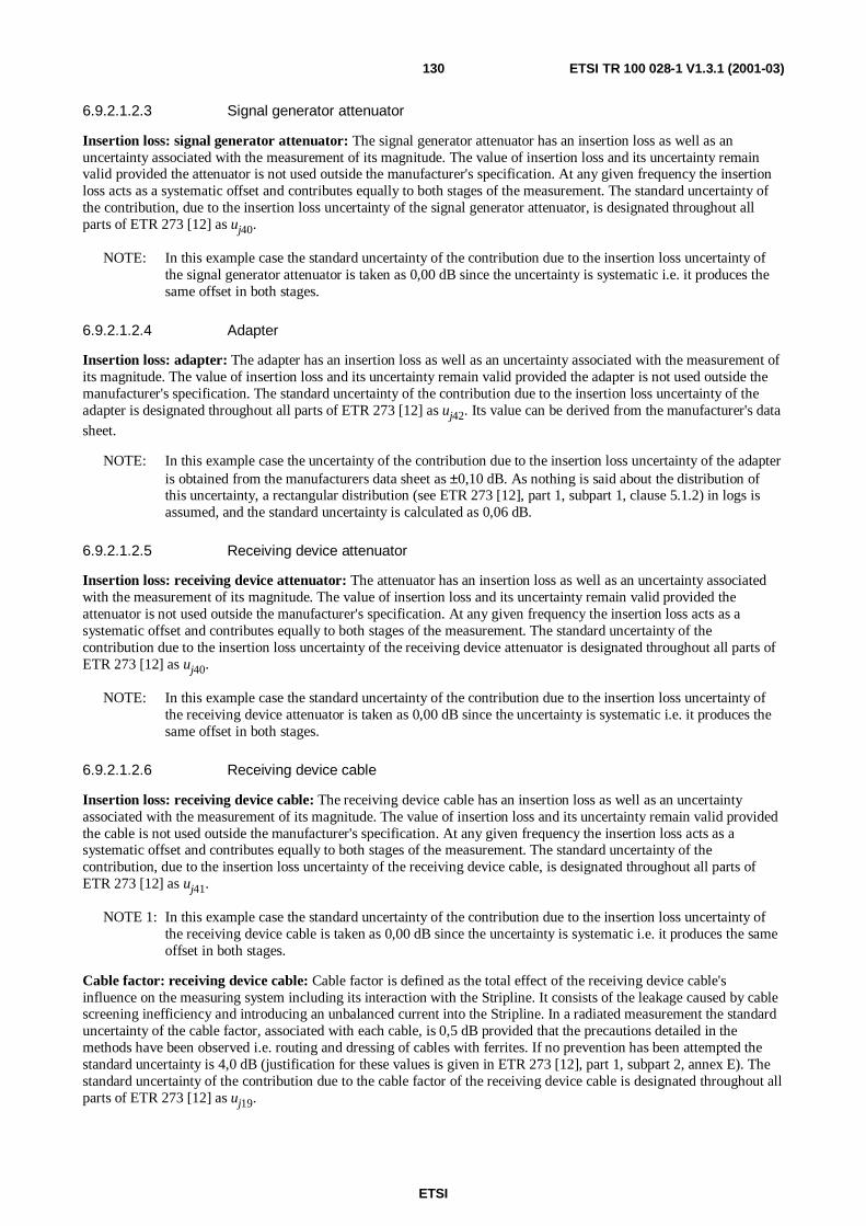
ETSI
ETSI TR 100 028-1 V1.3.1 (2001-03)130
6.9.2.1.2.3 Signal generator attenuator
Insertion loss: signal generator attenuator: The signal generator attenuator has an insertion loss as well as anuncertainty associated with the measurement of its magnitude. The value of insertion loss and its uncertainty remainvalid provided the attenuator is not used outside the manufacturer's specification. At any given frequency the insertionloss acts as a systematic offset and contributes equally to both stages of the measurement. The standard uncertainty ofthe contribution, due to the insertion loss uncertainty of the signal generator attenuator, is designated throughout allparts of ETR 273 [12] as uj40.
NOTE: In this example case the standard uncertainty of the contribution due to the insertion loss uncertainty ofthe signal generator attenuator is taken as 0,00 dB since the uncertainty is systematic i.e. it produces thesame offset in both stages.
6.9.2.1.2.4 Adapter
Insertion loss: adapter: The adapter has an insertion loss as well as an uncertainty associated with the measurement ofits magnitude. The value of insertion loss and its uncertainty remain valid provided the adapter is not used outside themanufacturer's specification. The standard uncertainty of the contribution due to the insertion loss uncertainty of theadapter is designated throughout all parts of ETR 273 [12] as uj42. Its value can be derived from the manufacturer's datasheet.
NOTE: In this example case the uncertainty of the contribution due to the insertion loss uncertainty of the adapteris obtained from the manufacturers data sheet as ±0,10 dB. As nothing is said about the distribution ofthis uncertainty, a rectangular distribution (see ETR 273 [12], part 1, subpart 1, clause 5.1.2) in logs isassumed, and the standard uncertainty is calculated as 0,06 dB.
6.9.2.1.2.5 Receiving device attenuator
Insertion loss: receiving device attenuator: The attenuator has an insertion loss as well as an uncertainty associatedwith the measurement of its magnitude. The value of insertion loss and its uncertainty remain valid provided theattenuator is not used outside the manufacturer's specification. At any given frequency the insertion loss acts as asystematic offset and contributes equally to both stages of the measurement. The standard uncertainty of thecontribution due to the insertion loss uncertainty of the receiving device attenuator is designated throughout all parts ofETR 273 [12] as uj40.
NOTE: In this example case the standard uncertainty of the contribution due to the insertion loss uncertainty ofthe receiving device attenuator is taken as 0,00 dB since the uncertainty is systematic i.e. it produces thesame offset in both stages.
6.9.2.1.2.6 Receiving device cable
Insertion loss: receiving device cable: The receiving device cable has an insertion loss as well as an uncertaintyassociated with the measurement of its magnitude. The value of insertion loss and its uncertainty remain valid providedthe cable is not used outside the manufacturer's specification. At any given frequency the insertion loss acts as asystematic offset and contributes equally to both stages of the measurement. The standard uncertainty of thecontribution, due to the insertion loss uncertainty of the receiving device cable, is designated throughout all parts ofETR 273 [12] as uj41.
NOTE 1: In this example case the standard uncertainty of the contribution due to the insertion loss uncertainty ofthe receiving device cable is taken as 0,00 dB since the uncertainty is systematic i.e. it produces the sameoffset in both stages.
Cable factor: receiving device cable: Cable factor is defined as the total effect of the receiving device cable'sinfluence on the measuring system including its interaction with the Stripline. It consists of the leakage caused by cablescreening inefficiency and introducing an unbalanced current into the Stripline. In a radiated measurement the standarduncertainty of the cable factor, associated with each cable, is 0,5 dB provided that the precautions detailed in themethods have been observed i.e. routing and dressing of cables with ferrites. If no prevention has been attempted thestandard uncertainty is 4,0 dB (justification for these values is given in ETR 273 [12], part 1, subpart 2, annex E). Thestandard uncertainty of the contribution due to the cable factor of the receiving device cable is designated throughout allparts of ETR 273 [12] as uj19.

ETSI
ETSI TR 100 028-1 V1.3.1 (2001-03)131
NOTE 2: In this example case the standard uncertainty of the contribution due to the cable factor of the receivingdevice cable is taken as 0,00 dB since there are no external fields involved other than leakage, which isassumed to have a negligible effect on the measurement.
6.9.2.1.2.7 Receiving device
In this, the first stage of the Stripline verification procedure, a reference level is set on the receiving device for aparticular output level from the signal generator. In the second stage (where the path loss through the Stripline ismeasured), a second level is obtained on the receiving device. Only in the second stage do the linearity and absolutelevel uncertainties of the receiver become involved in the calculation of the combined standard uncertainty for themeasurement.
Receiving device: absolute level: The standard uncertainty of the contribution due to the receiving device absolutelevel uncertainty is designated throughout all parts of ETR 273 [12] as uj47.
NOTE 1: In this example case the standard uncertainty of the contribution due to the absolute level uncertainty ofthe receiving device is assumed to be 0,00 dB since, in this part of the measurement, a reference level isrecorded.
Receiving device: linearity: The standard uncertainty of the contribution due to the receiving device linearity isdesignated throughout all parts of ETR 273 [12] as uj48.
NOTE 2: In this example case the standard uncertainty of the contribution due to the receiving device linearity isassumed to be 0,00 dB since, in this part of the measurement, a reference level is recorded.
6.9.2.1.3 Contribution from the random component
Random uncertainty: The magnitude can be assessed from multiple measurements of the direct attenuationmeasurement. The standard uncertainty of the contribution due to the random uncertainty is designated throughout allparts of ETR 273 [12] as ui01. Its value can then be calculated.
The direct attenuation measurement was repeated 10 times. The following results (dBµV) in were obtained (beforecorrecting for cabling and attenuator network insertion loss):
- 106,8; 107,2; 106,7; 107,0; 107,2; 106,7; 107,1; 106,8; 107,1; 107,0.
Converting to linear terms:
- 0,2188; 0,2291; 0,2163; 0,2239; 0,2291; 0,2163; 0,2265; 0,2188; 0,2265; 0,2239.
The two sums X and Y are calculated:
- X = the sum of the measured values = 2,2292 V;
- Y = the sum of the squares of the measured values = 0,4972 V2.
=−
−=
−
−=
11010
2292,24972,0
1
22
nn
XY
uc random 5,444 ×10-3 (formula 5.6)
As the result is obtained as the mean value of 10 measurements and the standard uncertainty of the random uncertaintyis:
dB0,2125,11
100
22292,0
10444,5 3=××=
−
j randomu
NOTE: In this example case the standard uncertainty of the contribution due to the random uncertainty is0,212 dB.

ETSI
ETSI TR 100 028-1 V1.3.1 (2001-03)132
6.9.2.1.4 Summary table of contributory components
A complete list of all the contributions to this part of the verification procedure is given in table 39.
Table 39: Contributions from the reference, direct measurement
uj or i Description of uncertainty contributions dBuj35 mismatch: direct attenuation measurement 0,03uj38 signal generator: absolute output level 0,00uj39 signal generator: output level stability 0,01uj41 insertion loss: signal generator cable 0,00uj19 cable factor: signal generator cable 0,00uj40 insertion loss: signal generator attenuator 0,00uj42 insertion loss: adapter 0,06uj40 insertion loss: receiving device attenuator 0,00uj41 insertion loss: receiving device cable 0,00uj19 cable factor: receiving device cable 0,00uj47 receiving device: absolute level 0,00uj48 receiving device: linearity 0,00ui01 random uncertainty 0,21
The standard uncertainties from table 39 should be combined by RSS in accordance with ETR 273 [12], part 1,subpart 1, clause 5. This gives the combined standard uncertainty (uc direct attenuation measurement) for the direct
attenuation measurement in dB.
The value of uc direct attenuation measurement is calculated as 0,223 dB.
6.9.2.2 Uncertainty contributions: Stage 2: Radiated attenuation measurement
The second stage of the verification procedure is the Stripline radiated attenuation measurement. This involvesmounting a monopole antenna through a hole in the lower plate of the Stripline, so that the feed point to the monopole isflush with the surface of the lower plate. The radiated attenuation measurement is carried out by removing the adapterand connecting the signal generator attenuator to the Stripline and connecting the receiving device attenuator to themonopole output (figure 35). The difference in received levels (after allowance for any correction factors which may beappropriate), for the same signal generator output level, is the Stripline radiated attenuation.
150termination
Load
Central axisof stripline
Ferrite beads10dB
attenuator
Ω
Receivingdevice
Signalgenerator
Figure 35: Stage 2: Radiated attenuation measurement
Whereas figure 35 shows, schematically, the test equipment set-up for this stage of the verification procedure, ananalysis diagram of the individual components (each of which contributes its own uncertainty) for this stage of themeasurement is shown in figure 36. Again, as stated above, the shaded areas represent components common to bothstages of the verification procedure.

ETSI
ETSI TR 100 028-1 V1.3.1 (2001-03)133
6.9.2.2.1 Contributions from the mismatch components
Mismatch in the transmitting and receiving parts: The value of the combined standard uncertainty of thecontributions due to the mismatch are calculated from the approach described in annex G. It is calculated in two parts.Firstly the standard uncertainty of the contribution due to the mismatch in the transmitting part, i.e. between the signalgenerator, cable, attenuator and the input to the Stripline and secondly, that for the receiving part, i.e. between thereceiving monopole antenna, attenuator, cable and the receiving device.
Signalgenerator
Cableloss
Cablefactor
Cableloss
Receivingdevice
Stripline
Signalgenerator
Signalgeneratorcable 1
Receivingdevice
cable 2
Attenuator 210 dB
Attenuator 110 dB
resonances, etc.
Cablefactor
Striplineto monopole
coupling
RadiatedLoss Monopole
Siteeffects
+
Receivingdevice
+
Room
Mismatch
Mismatch
Mismatch
Mismatch
Mismatch
Mismatch +
+ +
++
+
Figure 36: Stage 2: Radiated attenuation measurement
All the individual contributions are U-distributed.
NOTE 1: In this example value taken for the signal generator output reflection coefficient is the worst case over thefrequency band of interest, similarly, for the cable, adapter and attenuator VSWRs.
NOTE 2: The attenuation values of the cables and attenuators should be obtained from the data sheets/calibrationrecords at the specific frequency of the test, along with the associated uncertainties for these values.

ETSI
ETSI TR 100 028-1 V1.3.1 (2001-03)134
Mismatch: transmitting part:
Signal generator: Output reflection coefficient: |ρG| = 0,20
Cable: Input and output reflection coefficients: |S11| and |S22| = 0,07
Attenuation: 1 dB = |S12| = |S21| = 0,891
Attenuator: Input and output reflection coefficients |S11| = |S22| = 0,05
Attenuation = 10 dB |S12| = |S21| = 0,3162
Stripline: Input reflection coefficient: |ρSL| = 0,333
Those components that cancel are not calculated. Other contributions are (see annex G):
- uj mismatch: generator and cable 1: Constant for both stage 1 and 2. Hence this value does not contribute.
- uj mismatch: cable 1 and attenuator 1: Constant for both stage 1 and 2. Hence this value does not contribute.
%,1771%2
100333,005,01: =××=Striplineandattenuatormismatchju
- uj generator and attenuator 1: Constant for both stage 1 and 2. Hence this value does not contribute.
%0,165%2
100316,0333,007,0 2
1: =×××=Striplineandcablemismatchju
%0,373%2
100316,0891,0333,02,0 22
: =××××=Striplineandgeneratormismatchju
The combined standard uncertainty of the mismatch is then calculated:
%251373,0165,0177,1 222: ,u partngtransmittimismatchc =++=
transforming to the logarithmic form (ETR 028 [15], part 2, annex E): 1,25 %/11,5 = 0,11 dB.
The standard uncertainty of the contribution due to the mismatch in the transmitting part, is designated throughout allparts of ETR 273 [12] as uj36. Its value in this example is 0,11 dB.
Mismatch: receiving part:
Monopole: Input reflection coefficient: |ρM| = 0,333
Attenuator: Input and output reflection coefficients |S11| = |S22| = 0,05
Attenuation = 10 dB |S12| = |S21| = 0,3162
Cable: Input and output reflection coefficients: |S11| and |S22| = 0,07
Attenuation: 1 dB = |S12| = |S21| = 0,891
Receiving device: Output reflection coefficient: |ρRD| = 0,20
%,1771%2
10005,0333,0: =××=attenuatorandmonopolemismatchju
- uj attenuator 2 and cable 2: Constant for both stage 1 and 2. Hence this value does not contribute.
- uj cable 2 and receiving device: Constant for both stage 1 and 2. Hence this value does not contribute.
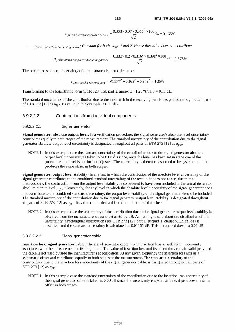
ETSI
ETSI TR 100 028-1 V1.3.1 (2001-03)135
%0,165%2
100316,007,0333,0 2
2: =×××=cableandmonopolemismatchju
- uj attenuator 2 and receiving device: Constant for both stage 1 and 2. Hence this value does not contribute.
%0,373%2
100891,0316,02,0333,0 22
: =××××=devicereceivingandmonopolemismatchju
The combined standard uncertainty of the mismatch is then calculated:
%251373,0165,0177,1 222: ,u partreceivingmismatchc =++=
Transforming to the logarithmic form (ETR 028 [15], part 2, annex E): 1,25 %/11,5 = 0,11 dB.
The standard uncertainty of the contribution due to the mismatch in the receiving part is designated throughout all partsof ETR 273 [12] as uj37. Its value in this example is 0,11 dB.
6.9.2.2.2 Contributions from individual components
6.9.2.2.2.1 Signal generator
Signal generator: absolute output level: In a verification procedure, the signal generator's absolute level uncertaintycontributes equally to both stages of the measurement. The standard uncertainty of the contribution due to the signalgenerator absolute output level uncertainty is designated throughout all parts of ETR 273 [12] as uj38.
NOTE 1: In this example case the standard uncertainty of the contribution due to the signal generator absoluteoutput level uncertainty is taken to be 0,00 dB since, once the level has been set in stage one of theprocedure, the level is not further adjusted. The uncertainty is therefore assumed to be systematic i.e. itproduces the same offset in both stages.
Signal generator: output level stability: In any test in which the contribution of the absolute level uncertainty of thesignal generator contributes to the combined standard uncertainty of the test i.e. it does not cancel due to themethodology, the contribution from the output level stability is considered to have been included in the signal generatorabsolute output level, uj38. Conversely, for any level in which the absolute level uncertainty of the signal generator does
not contribute to the combined standard uncertainty, the output level stability of the signal generator should be included.The standard uncertainty of the contribution due to the signal generator output level stability is designated throughoutall parts of ETR 273 [12] as uj39. Its value can be derived from manufacturers' data sheet.
NOTE 2: In this example case the uncertainty of the contribution due to the signal generator output level stability isobtained from the manufacturers data sheet as ±0,02 dB. As nothing is said about the distribution of thisuncertainty, a rectangular distribution (see ETR 273 [12], part 1, subpart 1, clause 5.1.2) in logs isassumed, and the standard uncertainty is calculated as 0,01155 dB. This is rounded down to 0,01 dB.
6.9.2.2.2.2 Signal generator cable
Insertion loss: signal generator cable: The signal generator cable has an insertion loss as well as an uncertaintyassociated with the measurement of its magnitude. The value of insertion loss and its uncertainty remain valid providedthe cable is not used outside the manufacturer's specification. At any given frequency the insertion loss acts as asystematic offset and contributes equally to both stages of the measurement. The standard uncertainty of thecontribution, due to the insertion loss uncertainty of the signal generator cable, is designated throughout all parts ofETR 273 [12] as uj41.
NOTE 1: In this example case the standard uncertainty of the contribution due to the insertion loss uncertainty ofthe signal generator cable is taken as 0,00 dB since the uncertainty is systematic i.e. it produces the sameoffset in both stages.

ETSI
ETSI TR 100 028-1 V1.3.1 (2001-03)136
Cable factor: signal generator cable: Cable factor is defined as the total effect of the signal generator cable's influenceon the measuring system including its interaction with the Stripline. It consists of the leakage caused by cable screeninginefficiency and introducing an unbalanced current into the Stripline. In a radiated measurement the standarduncertainty of the cable factor, associated with each cable, is 0,5 dB provided that the precautions detailed in themethods have been observed. i.e. routing and dressing of cables with ferrites. If no prevention has been attempted thestandard uncertainty is 4,0 dB (justification for these values is given in ETR 273 [12], part 1, subpart 2, annex E). Thestandard uncertainty of the contribution due to the cable factor of the signal generator cable is designated throughout allparts of ETR 273 [12] as uj19.
NOTE 2: In this example case the standard uncertainty of the contribution due to the cable factor of the transmittingantenna cable is taken as 0,50 dB since the precautions detailed in the methods are assumed to have beenobserved.
6.9.2.2.2.3 Signal generator attenuator
Insertion loss: signal generator attenuator: The signal generator attenuator has an insertion loss as well as anuncertainty associated with the measurement of its magnitude. The value of insertion loss and its uncertainty remainvalid provided the attenuator is not used outside the manufacturer's specification. At any given frequency the insertionloss acts as a systematic offset and contributes equally to both stages of the measurement. The standard uncertainty ofthe contribution, due to the insertion loss uncertainty of the signal generator attenuator, is designated throughout allparts of ETR 273 [12] as uj40.
NOTE: In this example case the standard uncertainty of the contribution due to the insertion loss uncertainty ofthe signal generator attenuator is taken as 0,00 dB since the uncertainty is systematic i.e. it produces thesame offset in both stages.
6.9.2.2.2.4 Site factors
Ambient effect: Uncertainty is introduced as a result of local ambient signals raising the noise floor at the measurementfrequency. The standard uncertainty of the contribution due to the ambient effect is designated throughout all parts ofETR 273 [12] as uj34. The values of the standard uncertainty should be taken from table 40.
Table 40: Uncertainty contribution: Ambient effect
Receiving device noise floor(generator OFF) is within:
Standard uncertainty ofthe contribution
3 dB of measurement 1,57 dB3 dB to 6 dB of measurement 0,80 dB6 dB to 10 dB of measurement 0,30 dB10 dB to 20 dB of measurement 0,10 dB20 dB or more of the measurement 0,00 dB
NOTE 1: In this example case the standard uncertainty of the contribution due to the ambient effect is taken as0,00 dB since the Stripline is assumed to be placed in a shielded room.
Stripline: influence of site effects: The influence of site effects comprise those effects resulting from not observing therecommendations given in EN 55020 [16] regarding positioning of the Stripline and layout of the absorber. These canlead to incorrect received levels i.e. values which differ from theoretical calculations. The standard uncertainty of thecontribution due to the influence of site effects is designated throughout all parts of ETR 273 [12] as uj33.
NOTE 2: In this example case the standard uncertainty of the contribution due to the influence of site effects istaken to have a standard uncertainty of 3,0 dB (see annex A). In the verification procedure, site effectsonly contribute to the Stripline radiated attenuation part.

ETSI
ETSI TR 100 028-1 V1.3.1 (2001-03)137
6.9.2.2.2.5 Antenna factor of the monopole
Stripline: antenna factor of the monopole: This has been derived from measurements taken within the Stripline.Therefore, the given values incorporate several of the field disturbance factors which the Stripline possesses and whichtherefore do not have to be allowed for as individual contributions. Amongst these included effects are imaging,characteristic impedance of the line, non-planar nature of the field etc. The standard uncertainty of the contribution dueto the antenna factor of the monopole is designated throughout all parts of ETR 273 [12] as uj30.
NOTE: In this example case the standard uncertainty of the contribution due to the antenna factor of themonopole is taken as 1,15 dB. This combined uncertainty source is only present in the Stripline radiatedattenuation measurement.
6.9.2.2.2.6 Receiving device attenuator
Insertion loss: receiving device attenuator: The receiving device attenuator has an insertion loss as well as anuncertainty associated with the measurement of its magnitude. The value of insertion loss and its uncertainty remainvalid provided the attenuator is not used outside the manufacturer's specification. At any given frequency the insertionloss acts as a systematic offset and contributes equally to both stages of the measurement. The standard uncertainty ofthe contribution due to the insertion loss uncertainty of the receiving device attenuator is designated throughout all partsof ETR 273 [12] as uj40.
NOTE: In this example case the standard uncertainty of the contribution due to the insertion loss uncertainty ofthe receiving device attenuator is taken as 0,00 dB since the uncertainty is systematic i.e. it produces thesame offset in both stages.
6.9.2.2.2.7 Receiving device cable
Insertion loss: receiving device cable: The receiving device cable has an insertion loss as well as an uncertaintyassociated with the measurement of its magnitude. The value of insertion loss and its uncertainty remain valid providedthe cable is not used outside the manufacturer's specification. At any given frequency the insertion loss acts as asystematic offset and contributes equally to both stages of the measurement. The standard uncertainty of thecontribution, due to the insertion loss uncertainty of the receiving device cable, is designated throughout all parts ofETR 273 [12] as uj41.
NOTE 1: In this example case the standard uncertainty of the contribution due to the insertion loss uncertainty ofthe receiving device cable is taken as 0,00 dB since the uncertainty is systematic i.e. it produces the sameoffset in both stages.
Cable factor: receiving device cable: Cable factor is defined as the total effect of the receiving device cable'sinfluence on the measuring system including its interaction with the site. It consists of the leakage caused by cablescreening inefficiency and introducing an unbalanced current into the monopole. In a radiated measurement thestandard uncertainty of the cable factor, associated with each cable, is 0,5 dB provided that the precautions detailed inthe methods have been observed i.e. routing and dressing of cables with ferrites. If no prevention has been attempted thestandard uncertainty is 4,0 dB (justification for these values is given in ETR 273 [12], part 1, subpart 2, annex E). Thestandard uncertainty of the contribution due to the cable factor of the receiving device cable is designated throughout allparts of ETR 273 [12] as uj19.
NOTE 2: In this example case the standard uncertainty of the contribution due to the cable factor of the receivingantenna cable is taken as 0,50 dB since the precautions detailed in the methods have been observed.
6.9.2.2.2.8 Receiving device
The first stage of the verification procedure involved setting a reference level on the receiving device for a particularoutput level from the signal generator. In this the second stage (where the radiated attenuation through the Stripline ismeasured), a second level is obtained which results in linearity and absolute level uncertainties becoming involved inthe calculation of the combined standard uncertainty for the measurement.
Receiving device: absolute level: This uncertainty only contributes during the second stage of the procedure if theinput attenuation range setting on the receiving device has been changed from its setting in the first stage. The standarduncertainty of the contribution due to the receiving device absolute level uncertainty is designated throughout all partsof ETR 273 [12] as uj47.

ETSI
ETSI TR 100 028-1 V1.3.1 (2001-03)138
NOTE 1: In this example case the uncertainty of the contribution due to the receiving device absolute leveluncertainty (a range change is assumed) is obtained from the manufacturers data as ±0,5 dB. As nothingis said about the distribution of this uncertainty, a rectangular distribution (see ETR 273 [12], part 1,subpart 1, clause 5.1.2) in logs is assumed. The standard uncertainty of the contribution due to thereceiving device absolute level uncertainty is calculated as 0,29 dB.
Receiving device: linearity: In any test in which the contribution of the absolute level uncertainty of the receivingdevice contributes to the combined standard uncertainty of the test i.e. it does not cancel due to the methodology, thecontribution from the receiving device linearity is considered to have been included in uj47. Conversely, for any test in
which the absolute level uncertainty of the receiving device does not contribute to the combined standard uncertaintythe linearity of the receiving device should be included. The standard uncertainty of the contribution due to thereceiving device linearity is designated throughout all parts of ETR 273 [12] as uj48.
NOTE 2: In this example case the standard uncertainty of the contribution due to the receiving device linearity istaken as 0,00 dB.
6.9.2.2.3 Contribution from the random component
Random uncertainty: The magnitude can be assessed from multiple measurements of the radiated attenuationmeasurement. The standard uncertainty of the contribution due to the random uncertainty is designated throughout allparts of ETR 273 [12] as ui01.
The radiated attenuation measurement was repeated 10 times. The following results were obtained in dBµV (beforecorrecting for cabling and attenuator network insertion loss):
- 65,4; 63,4; 66,0; 65,3; 63,0; 64,9; 65,2; 66,8; 65,5; 63,7.
Converting to linear terms:
- 1,862 × 10-3; 1,479 × 10-3; 1,995 × 10-3; 1,841 × 10-3; 1,413 × 10-3; 1,758 × 10-3; 1,820 × 10-3; 2,188 × 10-3;1,884 × 10-3; 1,531 × 10-3;
The two sums X and Y are calculated:
- X = the sum of the measured values = 17,77 × 10⁻³;
- Y = the sum of the squares of the measured values = 32,10 × 10⁻⁶ V2.
( )=
−
×−×=
−
−=
−−
11010
1077,171010,32
1
236
2
nn
XY
uc random 238,3 ×10⁻⁶ (formula 5.6)
As the result is obtained as the mean value of 10 measurements and the standard uncertainty of the random uncertaintyis:
dB1,175,11
100
10777,1
103,2383
6=×
×
×=−
−
j randomu
NOTE: In this example case the standard uncertainty of the contribution due to the random uncertainty is 1,17 dB.

ETSI
ETSI TR 100 028-1 V1.3.1 (2001-03)139
6.9.2.2.4 Summary table of contributory components
A complete list of all the contributions to this part of the verification procedure is given in table 41.
Table 41: Contributions from the radiated attenuation measurement
uj or i Description of uncertainty contributions dBuj36 mismatch: transmitting part 0,11uj37 mismatch: receiving part 0,11uj38 signal generator: absolute output level 0,00uj39 signal generator: output level stability 0,01uj41 insertion loss: signal generator cable 0,00uj19 cable factor: signal generator cable 0,50uj40 insertion loss: signal generator attenuator 0,00uj34 ambient effect 0,00uj33 Stripline: influence of site effects 3,00uj31 Stripline: antenna factor of the monopole 1,15uj40 insertion loss: receiving device attenuator 0,00uj41 insertion loss: receiving device cable 0,00uj19 cable factor: receiving device cable 0,50uj47 receiving device: absolute level 0,29uj48 receiving device: linearity 0,00ui01 random uncertainty 1,17
The standard uncertainties from table 41 should be combined by RSS in accordance with ETR 273 [12], part 1,subpart 1, clause 5. This gives the combined standard uncertainty (uc Stripline attenuation measurement) for the Stripline
attenuation measurement in dB.
The value of uc Stripline attenuation measurement is calculated as 3,51 dB.
6.9.2.2.5 Expanded uncertainty for the verification procedure
The combined standard uncertainty of the results of the verification procedure is the combination of the componentsoutlined in clauses 6.9.2.1.4 and 6.9.2.2.4. The components to be combined are uc direct attenuation measurement anduc Stripline attenuation measurement.
dB3,51=51,3223,0 22 +=procedureonverificatiStriplinecu
The expanded uncertainty is ±1,96 x 3,51 = ±6,89 dB at a 95 % confidence level.
6.9.3 Example 2: The measurement of a receiver parameter (Sensitivity)
For the measurement of receiver sensitivity two stages of test are involved. The first stage (determining the TransformFactor of the Stripline) involves measuring the field strength at the point where the receiver will be placed anddetermining the relationship between the signal generator output power level and the resulting field strength. Thesecond stage (the EUT measurement) involves placing the EUT within the Stripline and adjusting the output level of thesignal generator until the required response is obtained on the receiver. The signal generator output power level is thenconverted to field strength using the Transform Factor.

ETSI
ETSI TR 100 028-1 V1.3.1 (2001-03)140
6.9.3.1 Uncertainty contributions: Stage 1: EUT measurement
The first stage of the measurement is to determine the minimum signal generator output level which produces therequired response from the EUT. The test equipment set-up is shown in see figure 37.
150termination
Load
Central axisof stripline
Ferrite beads10dB
attenuator
Non-conducting,low dielectric constantsupport stand
EUT with volume centremidway between plates
Ω
Modulationdetection
Signalgenerator
Figure 37: Stage 1: EUT measurement
Whereas figure 37 shows, schematically, the test equipment set-up for the EUT sensitivity measurement, figure 38, ananalysis diagram, provides a detailed picture of the individual uncertainty components (each of which contributes itsown uncertainty) for this stage in the measurement. As stated above, the shaded areas represent components common toboth stages of the test method.
6.9.3.1.1 Contributions from the mismatch components
Mismatch: transmitting part: The uncertainty due to mismatch for the measurement on the EUT concerns only thesignal generator, the signal generator cable, the signal generator attenuator and the input to the Stripline. The mismatchuncertainty through this network does, however, contribute equally to both stages of the test for cases in which a fieldstrength measurement is subsequently performed.
If, however, the results of the verification procedure are used to calculate the field strength, the contribution of themismatch uncertainty needs to be calculated, from the approach described in annex G. All the contributions areU-distributed.
Signal generator: Output reflection coefficient: |ρG| = 0,20
Cable: Input and output reflection coefficients: |S11| and |S22| = 0,07
Attenuation: 1 dB = |S12| = |S21| = 0,891
Attenuator: Input and output reflection coefficients |S11| = |S22| = 0,05
Attenuation = 10 dB |S12| = |S21| = 0,3162
Stripline: Input reflection coefficient: |ρSL| = 0,333

ETSI
ETSI TR 100 028-1 V1.3.1 (2001-03)141
Signalgenerator
Cablefactor
Cableloss
Stripline
Signalgeneratorcable 1
Stripline toEUT
coupling
Signalgenerator
Signalgeneratorattenuator
Attenuator 110 dB
Modulationsource
Modulationdetector
Radiatedloss EUT
Room
Siteeffects
+
resonances, etc.
Mismatch
Mismatch
Mismatch
+
+
+
Figure 38: Schematic of the sensitivity measurement on the EUT
Mismatch: transmitting part.
All these contributions are U-distributed. Those components that cancel are not calculated. Other contributions are (seeannex G):
- uj mismatch: generator and cable 1: Constant for both stage 1 and 2. Hence this value does not contribute.
- uj mismatch: cable 1 and attenuator 1: Constant for both stage 1 and 2. Hence this value does not contribute.
%,1771%2
100333,005,01: =××=Striplineandattenuatormismatchju
- uj generator and attenuator 1: Constant for both stage 1 and 2. Hence this value does not contribute.
%0,165%2
100316,0333,007,0 2
1: =×××=Striplineandcablemismatchju

ETSI
ETSI TR 100 028-1 V1.3.1 (2001-03)142
%0,373%2
100316,0891,0333,02,0 22
: =××××=Striplineandgeneratormismatchju
The combined standard uncertainty of the mismatch is then calculated:
%251373,0165,0177,1 222: ,u partngtransmittimismatchc =++=
Transforming to the logarithmic form (ETR 028 [15], part 2, annex E): 1,25 %/11,5 = 0,11 dB.
The standard uncertainty of the contribution due to the mismatch in the transmitting part, is designated throughout allparts of ETR 273 [12] as uj36. Its value in this example is 0,11 dB.
6.9.3.1.2 Contributions from the individual components
6.9.3.1.2.1 Signal generator
Signal generator: absolute output level: In this test method, the uncertainty due to the setting of the signal generator'sabsolute output level contributes to both stages. In stage 1, the output level is individually adjusted at each of 8 differentpositioning angles whilst in stage 2, after an inspection (or calculation) of the 8 different values, the signal generator isset to a specific output level. The standard uncertainty of the contribution due to the signal generator absolute outputlevel uncertainty is designated throughout all parts of ETR 273 [12] as uj38. Its value can be obtained from the
manufacturer's data sheet.
NOTE 1: In this example case the uncertainty of the contribution due to the signal generator absolute output level isobtained from the manufacturers data sheet as ±1,0 dB. As nothing is said about the distribution of thisuncertainty, a rectangular distribution (see ETR 273 [12], part 1, subpart 1, clause 5.1.2) in logs isassumed, and the standard uncertainty is calculated as 0,58 dB.
Signal generator: output level stability: In any test in which the contribution of the absolute level uncertainty of thesignal generator contributes to the combined standard uncertainty of the test i.e. it does not cancel due to themethodology, the contribution from the output level stability is considered to have been included in the signal generatorabsolute output level, uj38. Conversely, for any level in which the absolute level uncertainty of the signal generator does
not contribute to the combined standard uncertainty, the output level stability of the signal generator should be included.The standard uncertainty of the contribution due to the signal generator output level stability is designated throughoutall parts of ETR 273 [12] as uj39. Its value can be derived from manufacturers' data sheet.
NOTE 2: In this example case the standard uncertainty of the contribution due to the signal generator output levelstability is taken as 0,0 dB as it is covered by the absolute level uncertainty.
6.9.3.1.2.2 Signal generator cable
Insertion loss: signal generator cable: The signal generator cable has an insertion loss as well as an uncertaintyassociated with the measurement of its magnitude. The value of insertion loss and its uncertainty remain valid providedthe cable is not used outside the manufacturer's specification. At any given frequency the insertion loss acts as asystematic offset and contributes equally to both stages of the measurement. The standard uncertainty of thecontribution due to the insertion loss uncertainty of the signal generator cable is designated throughout all parts ofETR 273 [12] as uj41.
NOTE 1: In this example case the standard uncertainty of the contribution due to the insertion loss uncertainty ofthe signal generator cable is taken as 0,20 dB as the results of the verification procedure have been usedto determine the field strength and this value has been taken from the manufacturer's or calibration data.
NOTE 2: If a field measurement had been performed using either a monopole of 3-axis probe the value would havebeen 0,00 dB as the uncertainty is systematic i.e. it produces the same offset in both stages.

ETSI
ETSI TR 100 028-1 V1.3.1 (2001-03)143
Cable factor: signal generator cable: Cable factor is defined as the total effect of the signal generator cable's influenceon the measuring system including its interaction with the site. It consists of the leakage caused by cable screeninginefficiency and introducing an unbalanced current into the Stripline. In a radiated measurement the standarduncertainty of the cable factor, associated with each cable, is 0,5 dB provided that the precautions detailed in themethods have been observed. i.e. routing and dressing of cables with ferrites. If no prevention has been attempted thestandard uncertainty is 4,0 dB (justification for these values is given in ETR 273 [12], part 1, subpart 2, annex E). Thestandard uncertainty of the contribution due to the cable factor of the signal generator cable is designated throughout allparts of ETR 273 [12] as uj19.
NOTE 3: In this example case the standard uncertainty of the contribution due to the cable factor of the signalgenerator cable is taken as 0,5 dB since the precautions detailed in the test method have been observed.
6.9.3.1.2.3 Signal generator attenuator
Insertion loss: signal generator attenuator: The signal generator attenuator has an insertion loss as well as anuncertainty associated with the measurement of its magnitude. The value of insertion loss and its uncertainty remainvalid provided the attenuator is not used outside the manufacturer's specification. At any given frequency the insertionloss acts as a systematic offset and contributes equally to both stages of the measurement. The standard uncertainty ofthe contribution due to the insertion loss of the signal generator attenuator is designated throughout all parts ofETR 273 [12] as uj40.
NOTE 1: In this example case the standard uncertainty of the contribution due to the insertion loss uncertainty ofthe signal generator cable is taken as 0,20 dB as the results of the verification procedure have been usedto determine the field strength and this value has been taken from the manufacturer's or calibration data.
NOTE 2: If a field measurement had been performed using either a monopole of 3-axis probe the value would havebeen 0,00 dB as the uncertainty is systematic i.e. it produces the same offset in both stages.
6.9.3.1.2.4 Site factors
Ambient effect: Uncertainty is introduced as a result of local ambient signals raising the noise floor at the measurementfrequency. The standard uncertainty of the contribution due to the ambient effect is designated throughout all parts ofETR 273 [12] as uj34. The value of the standard uncertainty is the same as for the second stage.
NOTE 1: In this example case the standard uncertainty of the contribution due to the ambient effect is taken as0,00 dB since the Stripline is assumed to have been placed in a shielded room.
Stripline: influence of site effects: The influence of site effects comprise those effects, resulting from not observingthe recommendations given in EN 55020 [16] regarding positioning of the Stripline and layout of absorber. These canlead to incorrect received levels i.e. values which differ from theoretical calculations. In this example, therecommendations are assumed not to have been fully observed. The standard uncertainty of the contribution due to theinfluence of site effects is designated throughout all parts of ETR 273 [12] as uj33.
NOTE 2: In this example case the standard uncertainty of the contribution due to the influence of site effects istaken as 3,0 dB since in the verification procedure, site effects only contribute to the Stripline attenuationpart and therefore do not cancel.
NOTE 3: If a field measurement had been performed using either a monopole of 3-axis probe the value would havebeen 0,00 dB as the uncertainty is systematic i.e. it produces the same offset in both stages.

ETSI
ETSI TR 100 028-1 V1.3.1 (2001-03)144
6.9.3.1.2.5 EUT
Stripline: mutual coupling of the EUT to its images in the plates: The magnitude is dependent on the EUT's size.The EUT is assumed to be positioned midway between the plates. The standard uncertainty of the contribution due tothe mutual coupling of the EUT to its images in the plates is designated throughout all parts of ETR 273 [12] as uj24. Its
value can be obtained from table 42.
Table 42: Uncertainty contribution of the mutual coupling of the EUT to its images in the plates
Size of the EUT relative to the plateseparation
Standard uncertainty ofthe contribution
size/separation < 33 % 1,15 dB33 % ≤ size/separation < 50 % 1,73 dB50 % ≤ size/separation < 70 % 2,89 dB70 % ≤ size/separation ≤ 87,5 % (max.) 5,77 dB
NOTE 1: In this example case the standard uncertainty of the contribution due to the mutual coupling of the EUT toits images in the plates is 1,15 dB since it is assumed the equipment size is < 33 % of the plate separation.
Stripline: characteristic impedance: This uncertainty contribution results from the difference between the free-spacewave impedance (377 Ω) for which the EUT had been developed and that for the Stripline (150 Ω). The standarduncertainty of the contribution due to the characteristic impedance of the Stripline is designated throughout all parts ofETR 273 [12] as uj26.
NOTE 2: In this example case the standard uncertainty of the contribution due to the characteristic impedance ofthe Stripline is taken as having a standard uncertainty of 0,58 dB.
Stripline: correction factor for the size of the EUT: This uncertainty is the result of changes in the intensity of theelectric field between the plates resulting from the presence, and metal content of the EUT. The larger the size of theEUT in the vertical plane of the Stripline, the greater the field intensification effect. Correction factors are suppliedwithin the test method, and the associated standard uncertainty of the contribution of the uncertainty due to thecorrection factor for the size of the EUT is designated throughout all parts of ETR 273 [12] as uj32. For EUT mountedcentrally in the Stripline, values can be obtained from table 43.
Table 43: Uncertainty contribution: Stripline: correction factor for the size of the EUT
Height of the EUT(in the E-plane) is:
Standard uncertainty of thecontribution
height < 0,2 m 0,30 dB0,2 m ≤ height < 0,4 m 0,60 dB0,4 m ≤ height ≤ 0,7 m 1,20 dB
NOTE 3: In this example case the standard uncertainty of the contribution of the uncertainty due to the correctionfactor for the size of the EUT is taken as 0,60 dB as the EUT is 0,22 m high.
EUT: mutual coupling to the power leads: This is the uncertainty associated with the influence (reflections, parasiticeffects, etc.) of the power leads on the EUT. The standard uncertainty associated with this effect is 0,5 dB provided thatthe precautions detailed in the methods have been observed. i.e. routing and dressing of cables with ferrites. If noprevention has been attempted the standard uncertainty is 2,0 dB. The standard uncertainty of the contribution due tothe mutual coupling of the EUT to the power leads is designated throughout all parts of ETR 273 [12] as uj54.
NOTE 4: In this example case the standard uncertainty of the contribution due to the mutual coupling of the EUT tothe power leads is taken as 0,5 dB since the precautions detailed in the methods have been observed.
Stripline: non-planar nature of the field distribution: This uncertainty results from the non-uniform amplitude andphase distribution of the electric field across the EUT. The non-uniformity results from room resonances, constructionalproblems, moding, reflections, etc. The standard uncertainty of the contribution due to the non-planar nature of the fielddistribution is designated throughout all parts of ETR 273 [12] as uj27.
NOTE 5: In this example case the standard uncertainty of the contribution due to the non-planar nature of the fielddistribution is taken as 0,29 dB.

ETSI
ETSI TR 100 028-1 V1.3.1 (2001-03)145
EUT: degradation measurement: This contribution is a RF level uncertainty associated with the uncertainty ofmeasuring 20 dB SINAD, 10-2 bit stream or 80 % message acceptance ratio. The standard uncertainty of thecontribution due to the EUT degradation measurement, designated throughout all parts of ETR 273 [12] as uj52, can be
obtained from ETR 028 [15].
NOTE 6: In this example case, the standard uncertainty of the contribution is obtained from ETR 028 [15] and itsvalue is 0,68 dB.
6.9.3.1.3 Contribution from the random component
Random uncertainty: The magnitude can be assessed from multiple measurements of the receiver sensitivitymeasurement. The standard uncertainty of the contribution due to the random uncertainty is designated throughout allparts of ETR 273 [12] as ui01.
The receiver sensitivity measurement was repeated 10 times. The following results were obtained in dBµV (beforecorrecting for cabling and attenuator network insertion loss):
- 65,4; 63,4; 66,0; 65,3; 63,0; 64,9; 65,2; 66,8; 65,5; 63,7.
Converting to linear terms:
- 1,862 × 10-3; 1,479 × 10-3; 1,995 × 10-3; 1,841 × 10-3; 1,413 × 10-3; 1,758 × 10-3; 1,820 × 10-3; 2,188 × 10-3;1,884 × 10-3; 1,531 × 10-3.
The two sums X and Y are calculated:
- X = the sum of the measured values = 17,77 × 10⁻³;
- Y = the sum of the squares of the measured values = 32,10 × 10⁻⁶ V2.
( )=
−
×−×=
−
−=
−−
11010
1077,171010,32
1
236
2
nn
XY
uc random 238,3 ×10⁻⁶ (formula 5.6)
As the result is obtained as the mean value of 10 measurements and the standard uncertainty of the random uncertaintyis:
dB,1715,11
100
10777,1
103,2383
6=×
×
×=−
−
j randomu
NOTE: In this example case the standard uncertainty of the contribution due to the random uncertainty is 1,17 dB.
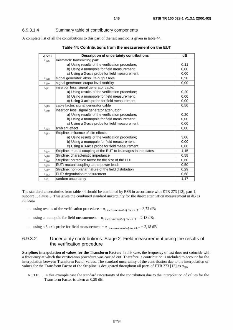
ETSI
ETSI TR 100 028-1 V1.3.1 (2001-03)146
6.9.3.1.4 Summary table of contributory components
A complete list of all the contributions to this part of the test method is given in table 44.
Table 44: Contributions from the measurement on the EUT
uj or i Description of uncertainty contributions dBuj36 mismatch: transmitting part:
a) Using results of the verification procedure;b) Using a monopole for field measurement;c) Using a 3-axis probe for field measurement.
0,110,000,00
uj38 signal generator: absolute output level 0,58uj39 signal generator: output level stability 0,00uj41 insertion loss: signal generator cable:
a) Using results of the verification procedure;b) Using a monopole for field measurement;c) Using 3-axis probe for field measurement.
0,200,000,00
uj19 cable factor: signal generator cable 0,50uj40 insertion loss: signal generator attenuator:
a) Using results of the verification procedure;b) Using a monopole for field measurement;c) Using a 3-axis probe for field measurement.
0,200,000,00
uj34 ambient effect 0,00uj33 Stripline: influence of site effects:
a) Using results of the verification procedure;b) Using a monopole for field measurement;c) Using a 3-axis probe for field measurement.
3,000,000,00
uj24 Stripline: mutual coupling of the EUT to its images in the plates 1,15uj26 Stripline: characteristic impedance 0,58uj32 Stripline: correction factor for the size of the EUT 0,60uj55 EUT: mutual coupling to the power leads 0,50uj27 Stripline: non-planar nature of the field distribution 0,29uj52 EUT: degradation measurement 0,68ui01 random uncertainty 1,17
The standard uncertainties from table 44 should be combined by RSS in accordance with ETR 273 [12], part 1,subpart 1, clause 5. This gives the combined standard uncertainty for the direct attenuation measurement in dB asfollows:
- using results of the verification procedure = uc measurement of the EUT = 3,72 dB;
- using a monopole for field measurement = uc measurement of the EUT = 2,18 dB;
- using a 3-axis probe for field measurement = uc measurement of the EUT = 2,18 dB.
6.9.3.2 Uncertainty contributions: Stage 2: Field measurement using the results ofthe verification procedure
Stripline: interpolation of values for the Transform Factor: In this case, the frequency of test does not coincide witha frequency at which the verification procedure was carried out. Therefore, a contribution is included to account for theinterpolation between Transform Factor values. The standard uncertainty of the contribution due to the interpolation ofvalues for the Transform Factor of the Stripline is designated throughout all parts of ETR 273 [12] as uj30.
NOTE: In this example case the standard uncertainty of the contribution due to the interpolation of values for theTransform Factor is taken as 0,29 dB.

ETSI
ETSI TR 100 028-1 V1.3.1 (2001-03)147
The appropriate standard uncertainties from table 44 should be combined with uj30 by RSS in accordance with
ETR 273 [12], part 1, subpart 1, clause 5. This gives the combined standard uncertainty (uc EUT measurement) for the EUTmeasurement in dB.
The value of uc EUT measurement is calculated as 3,56 dB.
6.9.3.2.1 Expanded uncertainty for the receiver sensitivity measurement
The combined standard uncertainty of the results of the receiver sensitivity measurement is the combination ofuc Stripline attenuation measurement and uc EUT measurement.
dB5,11=72,351,3 22 +=tmeasuremenysensitivitreceivercu
The expanded uncertainty is ±1,96 x 5,11= ±10,0 dB at a 95 % confidence level.
6.9.3.3 Uncertainty contributions: Stage 2: Field measurement using a monopole
The second stage involves replacing the EUT with a field measuring device (either a monopole antenna or a 3-axisprobe) and, setting a particular output level from the signal generator (minimum or average), measuring thecorresponding field strength, see figure 39.
NOTE: In this case monopole field measurement involves mounting the monopole through a hole in the lowerplate of the Stripline (so that the feed point to the monopole is flush with the surface of the lower plate)and measuring the field strength.
150termination
Load
Central axis ofStripline
Signalgenerator
Ferrite beads10dB
attenuators
ΩΩΩΩ
Monopole
Receivingdevice
Figure 39: Stage 2: Field measurement using a monopole
6.9.3.3.1 Contributions from the mismatch components
Mismatch in the transmitting and receiving parts: Whereas figure 39 shows schematically the equipment set-up forfield measurement using a monopole, figure 40 provides a detailed picture of the individual uncertainty contributions.
Mismatch: transmitting part: The mismatch uncertainty between the signal generator, signal generator cable, signalgenerator attenuator and the Stripline input can be calculated from the approach described in annex G. The mismatchuncertainty through this network does, however, contribute equally to both stages of the test for cases in which a fieldstrength measurement is subsequently performed since there are no changes from stage 1 to this part of the test set-up.The standard uncertainty of the contribution due to the mismatch in the transmitting part is designated throughout allparts of ETR 273 [12] as uj36.
NOTE 1: In this example case the standard uncertainty of the contribution due to mismatch in the transmitting partis taken as 0,00 dB, since the uncertainty is systematic i.e. it produces the same offset in both stages.
Mismatch: receiving part:
The mismatch uncertainty in the receiving part i.e. between the monopole, receiving device attenuator, receiving devicecable and the receiving device is calculated from the approach described in annex G. This mismatch uncertaintycontributes only during the field measurement part of the test and therefore contributes to the combined standarduncertainty.
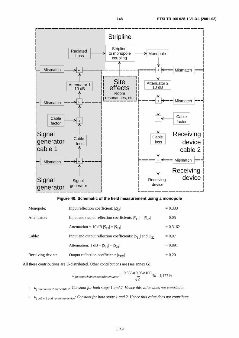
ETSI
ETSI TR 100 028-1 V1.3.1 (2001-03)148
Signalgenerator
Cableloss
Cablefactor
Cablefactor
Cableloss
Receivingdevice
Stripline
Receiving
Signalgenerator
device
Receivingdevice
cable 2
RadiatedLoss
Attenuator 110 dB
Signalgeneratorcable 1
Attenuator 210 dB
Striplineto monopole
couplingMonopole
+ Mismatch
Mismatch+
+
Mismatch+
+
Siteeffects
Roomresonances, etc.
Mismatch
Mismatch
Mismatch
+
+
+
Figure 40: Schematic of the field measurement using a monopole
Monopole: Input reflection coefficient: |ρM| = 0,333
Attenuator: Input and output reflection coefficients |S11| = |S22| = 0,05
Attenuation = 10 dB |S12| = |S21| = 0,3162
Cable: Input and output reflection coefficients: |S11| and |S22| = 0,07
Attenuation: 1 dB = |S12| = |S21| = 0,891
Receiving device: Output reflection coefficient: |ρRD| = 0,20
All these contributions are U-distributed. Other contributions are (see annex G):
%,1771%2
10005,0333,0: =××=attenuatorandantennamismatchju
- uj attenuator 2 and cable 2: Constant for both stage 1 and 2. Hence this value does not contribute.
- uj cable 2 and receiving device: Constant for both stage 1 and 2. Hence this value does not contribute.

ETSI
ETSI TR 100 028-1 V1.3.1 (2001-03)149
%0,165%2
100316,007,0333,0 2
2: =×××=cableandantennamismatchju
- uj attenuator 2 and receiving device: Constant for both stage 1 and 2. Hence this value does not contribute.
%0,373%2
100891,0316,02,0333,0 22
: =××××=devicereceivingandantennamismatchju
The combined standard uncertainty of the mismatch is then calculated:
%251373,0165,0177,1 222: ,u partreceivingmismatchj =++=
Transforming to the logarithmic form (ETR 028 [15], part 2, annex E): 1,25 %/11,5 = 0,11 dB.
The standard uncertainty of the contribution, due to the mismatch in the receiving part, is designated throughout allparts of ETR 273 [12] as uj37. Its value in this example is 0,11 dB.
6.9.3.3.2 Contributions from the individual components
6.9.3.3.2.1 Signal generator
Signal generator: absolute output level: In this test method, the uncertainty due to the setting of the signal generator'sabsolute output level contributes to both stages. In stage 1, the output level is individually adjusted at each of 8 differentpositioning angles whilst in stage 2, after an inspection (or calculation) of the 8 different values, the signal generator isset to a specific output level. The standard uncertainty of the contribution due to the signal generator absolute outputlevel is designated throughout all parts of ETR 273 [12] as uj38. Its value can be obtained from the manufacturer's data
sheet.
NOTE 1: In this example case the uncertainty of the contribution due to the signal generator absolute output leveluncertainty from the manufacturer's data sheet is ±1,0 dB. As nothing is said about the distribution of thisuncertainty, a rectangular distribution (see ETR 273 [12], part 1, subpart 1, clause 5.1.2) in logs isassumed, and the standard uncertainty is calculated as 0,58 dB.
Signal generator: output level stability: In any test in which the contribution of the absolute level uncertainty of thesignal generator contributes to the combined standard uncertainty of the test i.e. it does not cancel due to themethodology, the contribution from the output level stability is considered to have been included in the signal generatorabsolute output level, uj38. Conversely, for any level in which the absolute level uncertainty of the signal generator does
not contribute to the combined standard uncertainty, the output level stability of the signal generator should be included.The standard uncertainty of the contribution due to the signal generator output level stability is designated throughoutall parts of ETR 273 [12] as uj39. Its value can be derived from manufacturers' data sheet.
NOTE 2: In this example case the standard uncertainty of the contribution due to the signal generator output levelstability is taken as 0,00 dB as it is covered by the absolute level uncertainty.
6.9.3.3.2.2 Signal generator cable
Insertion loss: signal generator cable: The signal generator cable has an insertion loss as well as an uncertaintyassociated with the measurement of its magnitude. The value of insertion loss and its uncertainty remain valid providedthe cable is not used outside the manufacturer's specification. At any given frequency the insertion loss acts as asystematic offset and contributes equally to both stages of the measurement. The standard uncertainty of thecontribution due to the insertion loss uncertainty of the signal generator cable is designated throughout all parts ofETR 273 [12] as uj41.
NOTE 1: In this example case the standard uncertainty of the contribution due to the insertion loss uncertainty ofthe signal generator cable is taken as 0,00 dB since the uncertainty is systematic i.e. it is assumed constantand common to both stages of the measurement.

ETSI
ETSI TR 100 028-1 V1.3.1 (2001-03)150
Cable factor: signal generator cable: Cable factor is defined as the total effect of the signal generator cable's influenceon the measuring system including its interaction with the site. It consists of the leakage caused by cable screeninginefficiency and introducing an unbalanced current into the Stripline. In a radiated measurement the standarduncertainty of the uncertainty due to cable factor, associated with each cable, is 0,5 dB provided that the precautionsdetailed in the methods have been observed. i.e. routing and dressing of cables with ferrites. If no prevention has beenattempted the standard uncertainty is 4,0 dB (justification for these values is given in ETR 273 [12], part 1, subpart 2,annex E). The standard uncertainty of the contribution due to the cable factor of the signal generator cable is designatedthroughout all parts of ETR 273 [12] as uj19.
NOTE 2: In this example case the standard uncertainty of the contribution due to the cable factor of the signalgenerator cable is taken as 0,00 dB since the precautions detailed in the methods have been observed andthe field strength is to be measured.
6.9.3.3.2.3 Signal generator attenuator
Insertion loss: signal generator attenuator: The signal generator attenuator has an insertion loss as well as anuncertainty associated with the measurement of its magnitude. The value of insertion loss and its uncertainty remainvalid provided the attenuator is not used outside the manufacturer's specification. At any given frequency the insertionloss acts as a systematic offset and contributes equally to both stages of the measurement. The standard uncertainty ofthe contribution due to the insertion loss uncertainty of the signal generator attenuator is designated throughout all partsof ETR 273 [12] as uj40.
NOTE: In this example case the standard uncertainty of the contribution due to the insertion loss uncertainty ofthe signal generator attenuator is 0,00 dB since the precautions detailed in the methods have beenobserved and the field strength is to be measured.
6.9.3.3.2.4 Site factors
Ambient effect: Ambient effect is the uncertainty caused by local ambient signals raising the noise floor at themeasurement frequency. The standard uncertainty of the contribution due to the ambient effect is designated throughoutall parts of ETR 273 [12] as uj34. The value of the standard uncertainty should be taken from table 45.
Table 45: Uncertainty contribution: Ambient effect
Receiving device noise floor(EUT OFF) is within:
Standard uncertainty ofthe contribution
3 dB of measurement 1,57 dB3 dB to 6 dB of measurement 0,80 dB6 dB to 10 dB of measurement 0,30 dB10 dB to 20 dB of measurement 0,10 dB20 dB or more of the measurement 0,00 dB
NOTE 1: In this example case the standard uncertainty of the contribution due to the ambient effect is taken as0,00 dB since the Stripline is assumed to have been placed in a shielded room.
Stripline: influence of site effects: The influence of site effects comprise those effects, resulting from not observingthe recommendations given in EN 55020 [16] regarding positioning of the Stripline and layout of the absorber. Thesecan lead to incorrect received levels i.e. values which differ from theoretical calculations. The standard uncertainty ofthe contribution due to the influence of site effects is designated throughout all parts of ETR 273 [12] as uj33.
NOTE 2: In this example case the standard uncertainty of the contribution due to the influence of site effects istaken to be 0,00 dB since in this test method, site effects contribute equally to both stages as therecommendations are assumed to have been fully observed.

ETSI
ETSI TR 100 028-1 V1.3.1 (2001-03)151
6.9.3.3.2.5 Antenna factor of the monopole
Stripline: antenna factor of the monopole: This has been derived from measurements taken within the Stripline.Therefore, the given values incorporate several of the field disturbance factors which the Stripline possesses and whichtherefore do not have to be allowed for as individual contributions. Amongst these included effects are imaging,characteristic impedance of the line, non-planar nature of the field etc. The standard uncertainty of the contribution dueto the antenna factor of the monopole is designated throughout all parts of ETR 273 [12] as uj30.
NOTE: In this example case the standard uncertainty of the contribution due to the antenna factor of themonopole is taken as 1,15 dB. This combined uncertainty source is only present in the actualmeasurement.
6.9.3.3.2.6 Monopole attenuator
Insertion loss: Monopole attenuator: The monopole attenuator has an insertion loss as well as an uncertaintyassociated with the measurement of its magnitude. The value of insertion loss and its uncertainty remain valid providedthe attenuator is not used outside the manufacturer's specification. The standard uncertainty of the contribution due tothe insertion loss uncertainty of the monopole attenuator is designated throughout all parts of ETR 273 [12] as uj40.
NOTE: In this example case the standard uncertainty of the contribution due to the insertion loss uncertainty ofthe monopole attenuator is taken as 0,1 dB since the uncertainty contributes only to stage 2 of this testmethod.
6.9.3.3.2.7 Receiving device cable
Insertion loss: receiving device cable: The receiving device cable has an insertion loss as well as an uncertaintyassociated with the measurement of its magnitude. The value of insertion loss and its uncertainty remain valid providedthe cable is not used outside the manufacturer's specification. At any given frequency the insertion loss acts as asystematic offset and contributes equally to both stages of the measurement. The standard uncertainty of thecontribution due to the insertion loss uncertainty of the receiving device cable is designated throughout all parts ofETR 273 [12] as uj41.
NOTE 1: In this example case the standard uncertainty of the contribution due to the insertion loss uncertainty ofthe receiving device cable is taken as 0,15 dB since the uncertainty is only present in the second stage ofthis test method.
Cable factor: receiving device cable: Cable factor is defined as the total effect of the receiving device cable'sinfluence on the measuring system including its interaction with the site. It consists of the leakage caused by cablescreening inefficiency and introducing an unbalanced current into the monopole. In a radiated measurement thestandard uncertainty of the cable factor, associated with each cable, is 0,5 dB provided that the precautions detailed inthe methods have been observed. i.e. routing and dressing of cables with ferrites. If no prevention has been attemptedthe standard uncertainty is 4,0 dB (justification for these values is given in ETR 273 [12], part 1, subpart 2, annex E).The standard uncertainty of the contribution due to the cable factor of the receiving device cable is designatedthroughout all parts of ETR 273 [12] as uj19.
NOTE 2: In this example case the standard uncertainty of the contribution due to the cable factor of the receivingantenna cable is taken as 0,50 dB since the precautions detailed in the methods are assumed to have beenobserved.
6.9.3.3.2.8 Receiving device
Receiving device: absolute level: This uncertainty only contributes during the second stage of the procedure if theinput attenuation range setting on the receiving device has been changed from its setting in the first stage. The standarduncertainty of the contribution due to the receiving device absolute level uncertainty is designated throughout all partsof ETR 273 [12] as uj47.
NOTE 1: In this example case the standard uncertainty of the contribution due to the receiving device absolute leveluncertainty (a range change is assumed) is obtained from the manufacturers data as ±0,5 dB. As nothingis said about the distribution of this uncertainty, a rectangular distribution (see ETR 273 [12], part 1,subpart 1, clause 5.1.2) in logs is assumed, and the standard uncertainty is calculated as 0,29 dB.
ETSI
ETSI TR 100 028-1 V1.3.1 (2001-03)152
Receiving device: linearity: In any test in which the contribution of the absolute level uncertainty of the receivingdevice contributes to the combined standard uncertainty of the test i.e. it does not cancel due to the methodology, thecontribution from the receiving device linearity is considered to have been included in uj47. Conversely, for any test in
which the absolute level uncertainty of the receiving device does not contribute to the combined standard uncertaintythe linearity of the receiving device should be included. The standard uncertainty of the contribution due to thereceiving device linearity is designated throughout all parts of ETR 273 [12] as uj48.
NOTE 2: In this example case the standard uncertainty of the contribution due to the receiving device linearity istaken as 0,00 dB.
6.9.3.3.3 Contribution from the random component
Random uncertainty: The magnitude can be assessed from multiple measurements of the field strength measurement.The standard uncertainty of the contribution due to the random uncertainty is designated throughout all parts ofETR 273 [12] as ui01.
The field strength measurement was repeated 10 times. The following results were obtained in dBµV (before correctingfor cabling and attenuator network insertion loss):
- 65,4; 63,4; 66,0; 65,3; 63,0; 64,9; 65,2; 66,8; 65,5; 63,7.
Converting to linear terms:
- 1,862 × 10-3; 1,479 × 10-3; 1,995 × 10-3; 1,841 × 10-3; 1,413 × 10-3; 1,758 × 10-3; 1,820 × 10-3; 2,188 × 10-3;1,884 × 10-3; 1,531 × 10-3;
The two sums X and Y are calculated:
- X = the sum of the measured values = 17,77 × 10⁻³;
- Y = the sum of the squares of the measured values = 32,10 × 10⁻⁶ V2.
( )=
−
×−×=
−
−=
−−
11010
1077,171010,32
1
236
2
nn
XY
uc random 238,3 ×10⁻⁶ (formula 5.6)
As the result is obtained as the mean value of 10 measurements and the standard uncertainty of the random uncertaintyis:
dB,1715,11
100
10777,1
103,2383
6=×
×
×=−
−
j randomu
NOTE: In this example case the standard uncertainty of the contribution due to the random uncertainty is 1,17 dB.

ETSI
ETSI TR 100 028-1 V1.3.1 (2001-03)153
6.9.3.3.4 Summary table of contributions
A complete list of all the contributions to this part of the test method is given in table 46.
Table 46: Contributions from the monopole field measurement
uj or i Description of uncertainty contributions dBuj36 mismatch: transmitting part 0,00uj37 mismatch: receiving part 0,11uj38 signal generator: absolute output level 0,58uj39 signal generator: output level stability 0,00uj41 insertion loss: signal generator cable 0,00uj19 cable factor: signal generator cable 0,50uj40 insertion loss: signal generator attenuator 0,00uj34 ambient effect 0,00uj33 Stripline: influence of site effects 0,00uj31 Stripline: antenna factor of the monopole 1,15uj40 insertion loss: monopole attenuator 0,10uj41 insertion loss: receiving device cable 0,15uj19 cable factor: receiving device cable 0,50uj47 receiving device: absolute level 0,29uj48 receiving device: linearity 0,00ui01 random uncertainty 1,17
The standard uncertainties from table 46 should be combined by RSS in accordance with ETR 273 [12], part 1,subpart 1, clause 5. This gives the combined standard uncertainty (uc field measurement using a monopole) for the field
measurement using a monopole in dB.
The value of uc field measurement using a monopole is calculated as 1,91 dB.
6.9.3.3.5 Expanded uncertainty for the receiver sensitivity measurement
The combined standard uncertainty of the results of the receiver sensitivity measurement is the combination of thecomponents outlined in clauses 6.9.3.1.4 and 6.9.2.4.4. The components to be combined are uc measurement of the EUT anduc field measurement using a monopole.
dB2,90=91,118,2 22 +=cu
The expanded uncertainty is ±1,96 x 2,90 = ±5,68 dB at a 95 % confidence level.

ETSI
ETSI TR 100 028-1 V1.3.1 (2001-03)154
6.9.3.4 Uncertainty contributions: Stage 2: Field measurement using 3-axis probe
In this case, field measurement involves the use of a 3-axis probe and measuring the vertical component of the electricfield.
6.9.3.4.1 Contributions from the mismatch components
Whereas figure 41 shows schematically the equipment set-up for field measurement using a 3-axis probe, figure 42provides a detailed picture of the individual uncertainty contributions.
150termination
Load
Central axes of
Signalgenerator
Ferrite beads10dB
attenuatorΩΩΩΩ
Stripline3 axis probe
Digitalreadout
Figure 41: Stage 2: Field measurement using a 3-axis probe
Mismatch: transmitting part: The mismatch uncertainty between the signal generator, signal generator cable, signalgenerator attenuator and the Stripline input can be calculated from the approach described in annex G. The mismatchuncertainty through this network does, however, contribute equally to both stages of the test for cases in which a fieldstrength measurement is subsequently performed since there are no changes from stage 1 to this part of the test set-up.The standard uncertainty of the contribution due to the mismatch in the transmitting part is designated throughout allparts of ETR 273 [12] as uj36.
NOTE 1: In this example case the standard uncertainty of the contribution due to mismatch in the transmitting partis taken as 0,00 dB, since the uncertainty is systematic i.e. it produces the same offset in both stages.
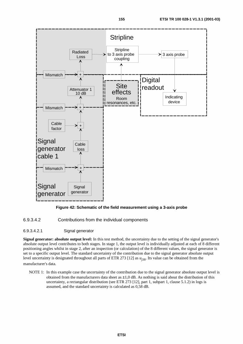
ETSI
ETSI TR 100 028-1 V1.3.1 (2001-03)155
Cablefactor
Cableloss
Stripline
Digitalreadout
Signalgenerator
Signalgeneratorcable 1
Signalgenerator
Attenuator 110 dB
RadiatedLoss
to 3 axis probeStripline
coupling
resonances, etc.
Siteeffects
Indicatingdevice
3 axis probe
+
Room
Mismatch
Mismatch
Mismatch
+
+
+
Figure 42: Schematic of the field measurement using a 3-axis probe
6.9.3.4.2 Contributions from the individual components
6.9.3.4.2.1 Signal generator
Signal generator: absolute output level: In this test method, the uncertainty due to the setting of the signal generator'sabsolute output level contributes to both stages. In stage 1, the output level is individually adjusted at each of 8 differentpositioning angles whilst in stage 2, after an inspection (or calculation) of the 8 different values, the signal generator isset to a specific output level. The standard uncertainty of the contribution due to the signal generator absolute outputlevel uncertainty is designated throughout all parts of ETR 273 [12] as uj38. Its value can be obtained from the
manufacturer's data.
NOTE 1: In this example case the uncertainty of the contribution due to the signal generator absolute output level isobtained from the manufacturers data sheet as ±1,0 dB. As nothing is said about the distribution of thisuncertainty, a rectangular distribution (see ETR 273 [12], part 1, subpart 1, clause 5.1.2) in logs isassumed, and the standard uncertainty is calculated as 0,58 dB.
ETSI
ETSI TR 100 028-1 V1.3.1 (2001-03)156
Signal generator: output level stability: In any test in which the contribution of the absolute level uncertainty of thesignal generator contributes to the combined standard uncertainty of the test i.e. it does not cancel due to themethodology, the contribution from the output level stability is considered to have been included in the signal generatorabsolute output level, uj38. Conversely, for any level in which the absolute level uncertainty of the signal generator does
not contribute to the combined standard uncertainty, the output level stability of the signal generator should be included.The standard uncertainty of the contribution due to the signal generator output level stability is designated throughoutall parts of ETR 273 [12] as uj39. Its value can be derived from manufacturers' data sheet.
NOTE 2: In this example case the standard uncertainty of the contribution due to the signal generator output levelstability is taken as 0,00 dB as it is covered by the absolute level uncertainty.
6.9.3.4.2.2 Signal generator cable
Insertion loss: signal generator cable: The signal generator cable has an insertion loss as well as an uncertaintyassociated with the measurement of its magnitude. The value of insertion loss and its uncertainty remain valid providedthe cable is not used outside the manufacturer's specification. At any given frequency the insertion loss acts as asystematic offset and contributes equally to both stages of the measurement. The standard uncertainty of thecontribution due to the insertion loss uncertainty of the signal generator cable is designated throughout all parts ofETR 273 [12] as uj41.
NOTE 1: In this example case the standard uncertainty of the contribution due to the insertion loss uncertainty ofthe signal generator cable is taken as 0,00 dB as a field strength measurement is performed using the3-axis probe.
Cable factor: signal generator cable: Cable factor is defined as the total effect of the signal generator cable's influenceon the measuring system including its interaction with the site. It consists of the leakage caused by cable screeninginefficiency and introducing an unbalanced current into the Stripline. In a radiated measurement the standarduncertainty of the uncertainty due to cable factor, associated with each cable, is 0,5 dB provided that the precautionsdetailed in the methods have been observed. i.e. routing and dressing of cables with ferrites. If no prevention has beenattempted the standard uncertainty is 4,0 dB (justification for these values is given in ETR 273 [12], part 1, subpart 2,annex E). The standard uncertainty of the contribution due to the cable factor of the signal generator cable is designatedthroughout all parts of ETR 273 [12] as uj19.
NOTE 2: In this example case the standard uncertainty of the contribution due to the cable factor of the signalgenerator cable is taken as 0,00 dB since the precautions detailed in the methods have been observed andthe field strength is to be measured.
6.9.3.4.2.3 Signal generator attenuator
Insertion loss: signal generator attenuator: The signal generator attenuator has an insertion loss as well as anuncertainty associated with the measurement of its magnitude. The value of insertion loss and its uncertainty remainvalid provided the attenuator is not used outside the manufacturer's specification. At any given frequency the insertionloss acts as a systematic offset and contributes equally to both stages of the measurement. The standard uncertainty ofthe contribution due to the insertion loss uncertainty of the signal generator attenuator is designated throughout all partsof ETR 273 [12] as uj40.
NOTE: In this example case the standard uncertainty of the contribution due to the insertion loss uncertainty ofthe signal generator attenuator is 0,00 dB since the precautions detailed in the methods have beenobserved and the field strength is to be measured.
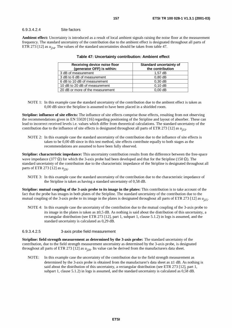
ETSI
ETSI TR 100 028-1 V1.3.1 (2001-03)157
6.9.3.4.2.4 Site factors
Ambient effect: Uncertainty is introduced as a result of local ambient signals raising the noise floor at the measurementfrequency. The standard uncertainty of the contribution due to the ambient effect is designated throughout all parts ofETR 273 [12] as uj34. The values of the standard uncertainties should be taken from table 47.
Table 47: Uncertainty contribution: Ambient effect
Receiving device noise floor(generator OFF) is within:
Standard uncertainty ofthe contribution
3 dB of measurement 1,57 dB3 dB to 6 dB of measurement 0,80 dB6 dB to 10 dB of measurement 0,30 dB10 dB to 20 dB of measurement 0,10 dB20 dB or more of the measurement 0,00 dB
NOTE 1: In this example case the standard uncertainty of the contribution due to the ambient effect is taken as0,00 dB since the Stripline is assumed to have been placed in a shielded room.
Stripline: influence of site effects: The influence of site effects comprise those effects, resulting from not observingthe recommendations given in EN 55020 [16] regarding positioning of the Stripline and layout of absorber. These canlead to incorrect received levels i.e. values which differ from theoretical calculations. The standard uncertainty of thecontribution due to the influence of site effects is designated throughout all parts of ETR 273 [12] as uj33.
NOTE 2: In this example case the standard uncertainty of the contribution due to the influence of site effects istaken to be 0,00 dB since in this test method, site effects contribute equally to both stages as therecommendations are assumed to have been fully observed.
Stripline: characteristic impedance: This uncertainty contribution results from the difference between the free-spacewave impedance (377 Ω) for which the 3-axis probe had been developed and that for the Stripline (150 Ω). Thestandard uncertainty of the contribution due to the characteristic impedance of the Stripline is designated throughout allparts of ETR 273 [12] as uj26.
NOTE 3: In this example case the standard uncertainty of the contribution due to the characteristic impedance ofthe Stripline is taken as having a standard uncertainty of 0,58 dB.
Stripline: mutual coupling of the 3-axis probe to its image in the plates: This contribution is to take account of thefact that the probe has images in both plates of the Stripline. The standard uncertainty of the contribution due to themutual coupling of the 3-axis probe to its image in the plates is designated throughout all parts of ETR 273 [12] as uj25.
NOTE 4: In this example case the uncertainty of the contribution due to the mutual coupling of the 3-axis probe toits image in the plates is taken as ±0,5 dB. As nothing is said about the distribution of this uncertainty, arectangular distribution (see ETR 273 [12], part 1, subpart 1, clause 5.1.2) in logs is assumed, and thestandard uncertainty is calculated as 0,29 dB.
6.9.3.4.2.5 3-axis probe field measurement
Stripline: field strength measurement as determined by the 3-axis probe: The standard uncertainty of thecontribution, due to the field strength measurement uncertainty as determined by the 3-axis probe, is designatedthroughout all parts of ETR 273 [12] as uj28. Its value can be derived from the manufacturers data sheet.
NOTE: In this example case the uncertainty of the contribution due to the field strength measurement asdetermined by the 3-axis probe is obtained from the manufacturer's data sheet as ±1 dB. As nothing issaid about the distribution of this uncertainty, a rectangular distribution (see ETR 273 [12], part 1,subpart 1, clause 5.1.2) in logs is assumed, and the standard uncertainty is calculated as 0,58 dB.

ETSI
ETSI TR 100 028-1 V1.3.1 (2001-03)158
6.9.3.4.3 Contribution from the random component
Random uncertainty: The magnitude can be assessed from multiple measurements of the receiver sensitivity. Thestandard uncertainty of the contribution due to the random uncertainty is designated throughout all parts ofETR 273 [12] as ui01.
The field strength measurement was repeated 10 times. The following results were obtained in dBµV (before correctingfor cabling and attenuator network insertion loss):
- 65,4; 63,4; 66,0; 65,3; 63,0; 64,9; 65,2; 66,8; 65,5; 63,7.
Converting to linear terms:
- 1,862 × 10-3; 1,479 × 10-3; 1,995 × 10-3; 1,841 × 10-3; 1,413 × 10-3; 1,758 × 10-3; 1,820 × 10-3; 2,188 × 10-3;1,884 × 10-3; 1,531 × 10-3;
The two sums X and Y are calculated:
- X = the sum of the measured values = 17,77 × 10⁻³;
- Y = the sum of the squares of the measured values = 32,10 × 10⁻⁶ V2.
( )=
−
×−×=
−
−=
−−
11010
1077,171010,32
1
236
2
nn
XY
uc random 238,3 ×10⁻⁶ (formula 5.6)
As the result is obtained as the mean value of 10 measurements and the standard uncertainty of the random uncertaintyis:
dB1,175,11
100
10777,1
103,2383
6=×
×
×=−
−
j randomu
NOTE: In this example case the standard uncertainty of the contribution due to the random uncertainty is 1,17 dB.
6.9.3.4.4 Summary table of contributory components
A complete list of all the contributions to this part of the test method is given in table 48.
Table 48: Contributions from the 3-axis probe field measurement
uj or i Description of uncertainty contributions dBuj36 mismatch: transmitting part 0,00uj38 signal generator: absolute output level 0,58uj39 signal generator: output level stability 0,00uj41 insertion loss: signal generator cable 0,00uj19 cable factor: signal generator cable 0,50uj40 insertion loss: signal generator attenuator 0,00uj34 ambient effect 0,00uj33 Stripline: influence of site effects 0,00uj26 Stripline: characteristic impedance 0,58uj25 Stripline: mutual coupling of the 3-axis probe to its image in the plates 0,29uj28 Stripline: field strength measurement as determined by the 3-axis probe 0,58ui01 random uncertainty 1,17
The standard uncertainties from table 48 should be combined by RSS in accordance with ETR 273 [12], part 1,subpart 1, clause 5. This gives the combined standard uncertainty (uc 3-axis probe) for the receiver sensitivity
measurement in dB.
The value of uc 3-axis probe is calculated as 1,65 dB.
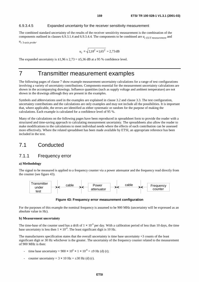
ETSI
ETSI TR 100 028-1 V1.3.1 (2001-03)159
6.9.3.4.5 Expanded uncertainty for the receiver sensitivity measurement
The combined standard uncertainty of the results of the receiver sensitivity measurement is the combination of thecomponents outlined in clauses 6.9.3.1.4 and 6.9.3.4.4. The components to be combined are uc EUT measurement and
uc 3-axis probe.
dB2,73=65,118,2 22 +=cu
The expanded uncertainty is ±1,96 x 2,73 = ±5,36 dB at a 95 % confidence level.
7 Transmitter measurement examplesThe following pages of clause 7 show example measurement uncertainty calculations for a range of test configurationsinvolving a variety of uncertainty contributions. Components essential for the measurement uncertainty calculations areshown in the accompanying drawings. Influence quantities (such as supply voltage and ambient temperature) are notshown in the drawings although they are present in the examples.
Symbols and abbreviations used in the examples are explained in clause 3.2 and clause 3.3. The test configuration,uncertainty contributions and the calculations are only examples and may not include all the possibilities. It is importantthat, where applicable, the errors are identified as either systematic or random for the purpose of making thecalculations. Each example is calculated for a confidence level of 95 %.
Many of the calculations on the following pages have been reproduced in spreadsheet form to provide the reader with astructured and time-saving approach to calculating measurement uncertainty. The spreadsheets also allow the reader tomake modifications to the calculations to meet individual needs where the effects of each contribution can be assessedmore effectively. Where the related spreadsheet has been made available by ETSI, an appropriate reference has beenincluded in the text.
7.1 Conducted
7.1.1 Frequency error
a) Methodology
The signal to be measured is applied to a frequency counter via a power attenuator and the frequency read directly fromthe counter (see figure 43).
Powerattenuator
Frequencycounter
cable cableTransmitterundertest
Figure 43: Frequency error measurement configuration
For the purposes of this example the nominal frequency is assumed to be 900 MHz (uncertainty will be expressed as anabsolute value in Hz).
b) Measurement uncertainty
The time-base of the counter used has a drift of 1 × 10⁻⁹ per day. With a calibration period of less than 10 days, the timebase uncertainty is less then 1 × 10⁻⁸. The least significant digit is 10 Hz.
The manufacturers specification states that the overall uncertainty is time base uncertainty +3 counts of the leastsignificant digit or 30 Hz whichever is the greater. The uncertainty of the frequency counter related to the measurementof 900 MHz is then:
- time base uncertainty = 900 × 106 × 1 × 10-8 = ±9 Hz (d) (r);
- counter uncertainty = 3 × 10 Hz = ±30 Hz (d) (r).

ETSI
ETSI TR 100 028-1 V1.3.1 (2001-03)160
There is also an uncertainty associated with the ambient temperature uncertainty. The dependency values found intable F.1 are:
- mean value of 0,02 ppm/°C;
- standard deviation of 0,01 ppm/°C.
This gives:
- 20 × 10-9 Hz/°C × 900 × 106 = 18 Hz/°C; and
- 10 × 10-9 Hz/°C × 900 × 106 = 9 Hz/°C.
Ambient temperature uncertainty is ± 3 °C (d) (r).
The standard uncertainty of the ambient temperature is:
CC
u tambj °=°
= 73,13
3
The ambient temperature uncertainty is converted to a frequency uncertainty by means of formula 5.2.
Hz))CHz/+()CHz/(()C,(u uncertambientj 8,34918731 222 =°°×°
Finally the combined standard uncertainty is calculated:
Hz)Hz+())Hz+()Hz((
=u errorfrequencyc 2,398,343
309 222
=
Using an expansion factor (coverage factor) of k = 1,96, the expanded measurement uncertainty is ±1,96 ×39,2 Hz = ±76,8 Hz (see annex D, clause D.5.6.2 in part 2).
c) Spreadsheet implementation of measurement uncertainty
This calculation has been implemented in a corresponding spreadsheet (see file "Frequency error.xls") and is availablein tr_10002801v010301p0.zip.
7.1.2 Carrier power
a) Methodology
The measurement is conducted using a power meter that consists of a thermocouple power sensor and a meter with abuilt in reference source. A 30 dB power attenuator is used to reduce the level applied to the sensor (see figure 44a).Before making the measurement, the loss of the cable and power attenuator are determined using a signal generator.The loss is measured by firstly connecting the generator to the power meter to obtain an arbitrary reference (seefigure 44b). The cable and attenuator are then inserted between the sensor and generator and the loss determined (seefigure 44c). Carrier power is recorded as the level measured on the power meter plus the measured correction for thecable and attenuator.
Transmitterunder test
PowermeterSensor
30dB powerattenuator
Cable
Power refsource
Figure 44a: Carrier Power measurement configuration
NOTE 1: An additional example of carrier power uncertainty involving two attenuators can be found in clause 6.4.
b) Measurement uncertainty

ETSI
ETSI TR 100 028-1 V1.3.1 (2001-03)161
i) Power meter and sensor:
power meter reference source level uncertainty is ±1,2 % (p) (d) (r).
dBu levelreferencej 03,00,233
2,1 =×
=
Calibration factor uncertainty = ±2,3 % (p) (d) (r).
dBu factorncalibratioj 058,00,233
3,2 =×
=
Range change error (one change) = ±0,5 % (p) (d) (r).
dBu changerangej 013,00,233
5,0 =×
=
Linearity factor = ±0,5 % (p) (d) (r).
dBu factorlinearityj 013,00,233
5,0 =×
=
Mismatch uncertainty when calibrating:
- reference source VSWRg = 1,05 (d) so reflection coefficient = 0,024;
- sensor input VSWRl = 1,15 (d) so reflection coefficient = 0,070.
dBu 01,05,112
10007,0024,0mismatchncalibratioj =
×××=
Noise and drift is negligible at this power level and can be ignored.
22222mismatchcaljfactorlinjchangerangejfactorcaljlevelrefjsensorandmeterpowerc uuuuu=u ++++
dB=u sensorandmeterpowerc 069,001,0013,0013,0058,003,0 22222 =++++
ii) Uncertainty when measuring the attenuator/cable loss:
RF signalgenerator
PowermeterSensor
Figure 44b: Determining the reference level
RF signalgenerator
PowermeterSensor
30dB powerattenuator
Cable
Figure 44c: measuring the attenuator and cable loss
Mismatch uncertainty:
- generator reflection coefficient is 0,07 (d);
- sensor reflection coefficient is 0,07 (d);
- cable reflection coefficients are 0,14 (d);
- attenuator reflection coefficients are 0,13 (d).

ETSI
ETSI TR 100 028-1 V1.3.1 (2001-03)162
For the calculation of mismatch uncertainty the cable attenuation is assumed to be 0 dB (x1 linear).
The mismatch uncertainty is comprised of two parts:
PART 1 - the reference measurement, this is when the generator and sensor are connected together (see figure 44b):
dB,,,
03005,112
100070070u tmeasuremenreference:mismatchj =
×××=
PART 2 - the attenuation measurement, this is when the cable and attenuator are placed between the generator andsensor (see figure 44c). Mismatch components appear at the generator/cable junction and the attenuator/sensor junction:
dB,,,
06005,112
100140070u cabletogenerator:mismatchj =
×××=
dB,,
05605,112
10007,0130u sensortoattenuator:mismatchj =
×××=
dB,,
05605,112
100113,0070u
2
attenuatortogenerator:mismatchj =×
×××=
NOTE 2: The remaining mismatch contributions have a negligible effect due to the isolating effect of the 30dBattenuator and have therefore been ignored.
The total mismatch uncertainty during the cable/attenuator measurement is:
2sensortogenertorj
2sensortoattenj
2cabletogeneratorj
2tmeasuremenreferencejtmeasuremennattenuatio:mismatchc uuuuu +++=
dB104,0056,0056,0060,0030,0u 2222tmeasuremennattenuatio:mismatchc =+++=
The 30dB attenuator will reduce the level at the sensor so:
2:
22tmeasuremennattenuatiomismatchcfactorlinearityjerrorchangerangejntmeasuremeattenuatorandc cable uuuu ++=
dB106,0104,0013,0013,0u 222tmeasuremenattenuatorandcablec =++=
iii) Carrier power measurement (see fig 44a):
Attenuator uncertainty:
Temperature influence = 0,0001 dB/degree which is negligible and can be ignored.
Power influence on the attenuator is 0,001 dB/dB x Watt (d) (r) = 0,001 x 30 x 25 = 0,75 dB (r):
dB,,
43303
750u influencepowerj ==
Mismatch uncertainty:
- transmitter reflection coefficient is 0.5 (taken from table F.1);
- cable reflection coefficients are 0,14 (d);
- attenuator reflection coefficients are 0,13 (d);
- sensor reflection coefficient is 0,07 (d).
For the calculation of mismatch uncertainty the cable attenuation is assumed to be 0 dB (x 1 linear).
dB,
430,05,112
%10014,050u cabletoEUT:mismatchj =
×××=

ETSI
ETSI TR 100 028-1 V1.3.1 (2001-03)163
dB,
400,05,112
%100113,050u
2
attenuatortoEUT:mismatchj =×
×××=
dB056,05,112
%10007,013,0u sensortoattenuator:mismatchj =
×××=
The total mismatch uncertainty during the power measurement is:
2sensortoattenuatorj
2attenuatortoEUTj
2cabletoEUTjtmeasuremenpower:mismatchc uuuu ++=
dB60,0056,0400,0430,0u 222tmeasuremenpower:mismatchc =++=
NOTE 3: The remaining mismatch contributions have a negligible effect due to the isolating effect of the 30dBattenuator and have therefore been ignored.
Uncertainty due to influence quantities:
Ambient temperature = 20°C ± 1°C (d) (r).
The ambient temperature uncertainty is converted to a level uncertainty by means of formula 5.2 and table F.1.Dependency values found in table F.1 are:
- mean of 4 % power/°C;
- standard deviation of 1,2 % power/°C.
Therefore:
dB=
))C% /,+()C% /,(()C(
u 1,023
21043
1 222
yuncertaintetemperaturj
°°×
°
=
Supply voltage = Vset ± 100 mV (d) (r).
The supply voltage uncertainty is converted to a level uncertainty by means of formula 5.2 and table F.1. Dependencyvalues found in table F.1 are:
- mean value of 10 % power/V;
- standard deviation of 3 % power/V.
Therefore:
dB
))V/%(3+)V/%((103
)(0,1V
u
222
026,023yuncertaintvoltagesupplyj =
×
=
Random uncertainty:
The measurement was repeated 9 times with the following results:
- 21,8 mW; 22,8 mW; 23,0 mW; 22,5 mW; 22,1 mW; 22,7 mW; 21,7 mW; 22,3 mW; 22,7 mW.
Mean value = 22,4 mW, standard deviation = 0,455 mW.
As the result is obtained as the mean value of 9 measurements the normalized standard deviation of the randomuncertainty is:
dB=%100922,4mW
0,455mWu randomi 03,0
0,23×
××=

ETSI
ETSI TR 100 028-1 V1.3.1 (2001-03)164
Uncertainty due to time duty cycle:
The standard uncertainty of the time duty cycle error (found in table F.1) = 2 % (p) (σ).
dBu cycledutytimej 087,00,23
%2 ==
2cycledutytimej
2randomi
2voltagesupplyj
2tempj
2tmeasuremenPowermismatch:c
2influencepwrjtmeasuremenpowerc uuuuuu=u +++++
dB=,= 75,0087,0030026,01,06,0433,0u 222222tmeasuremenpowerc +++++
The combined standard uncertainty for carrier power is:
2tmeasuremenpowerc
2tmeasuremenattenuator&cablec
2sensor&meterpowercpowercarrierc uuu=u ++
dB=,= 76,075,0106,00690u 222powercarrierc ++
Using an expansion factor (coverage factor) of k = 1,96, the expanded measurement uncertainty is ±1,96 ×0,76dB = ±1,49dB (see annex D, clause D.5.6.2 in part 2).
c) Spreadsheet implementation of measurement uncertainty
This calculation has been implemented in a corresponding spreadsheet (see file "Carrier power_Rev1.xls") and isavailable in tr_10002801v010301p0.zip.
7.1.3 Adjacent channel power
7.1.3.1 Adjacent channel power method 1 (Using an adjacent channel power meter)
a) Methodology
The transmitter under test is connected to an adjacent channel power meter (power measuring receiver) via an attenuator(see figure 45).
cablecable Powerattenuator
Transmitterundertest
ModulatingAF oscillator
Low noise RFsignal generator
Powermeasuringreceiver
Figure 45: Measurement configuration for adjacent channel power measurement (method 1)
b) Measurement uncertainty
Power bandwidth of measuring receiver filter = ±0,2 dB (d) (r).
0,115dB3
20,0 =±=bandwidthfilterju
Relative accuracy of measuring receiver = ±0,5 dB (d) (r).
0,289dB3
50,0 =±=accuracyrelativeju

ETSI
ETSI TR 100 028-1 V1.3.1 (2001-03)165
Standard uncertainty of the random error = 0,11 dB (σ).
u i random = 0,11 dB
Deviation uncertainty = ±30 Hz (d) (r).
Deviation uncertainty is converted to a relative adjacent channel power uncertainty by means of formula 5.2 andtable F.1. Dependency values found in table F.1 are:
- mean value of 0,05 % (p) / Hz;
- standard deviation of 0,02 % (p) / Hz.
Therefore:
( ) ( ) ( )( )dB=
% / Hz,% / Hz,Hz
u deviationconvertedj 04,00,23
0200503
30 222
+×
=
Uncertainty caused by measuring receiver filter position.
Uncertainty of 6 dB point = ±75 Hz (d) (r).
The uncertainty of the 6dB point is converted to a relative adjacent channel power uncertainty by means of formula 5.2and table F.1. Dependency values found in table F1 are:
- mean value of 15 dB/kHz;
- standard deviation of 4 dB/kHz.
Therefore:
dB))dB/kHz+()dB/kHz(()kHz,(
u positionfilterconvertedj 67,04153
0750 222
=×
=
22222posfilterconvertedjdevconvertedjrandomiaccuracyrelativejbwpwrfilterjpowerchanneldjacentac uuuuuu ++++=
0,748dB67,004,011,0289,0115,0 22222 =++++=powerchanneladjacentcu
Using an expansion factor (coverage factor) of k = 1,96, the expanded measurement uncertainty is ±1,96 × 0,748 dB= ±1,47dB (see annex D, clause D.5.6.2 in part 2).
c) Spreadsheet implementation of measurement uncertainty
This calculation has been implemented in a corresponding spreadsheet (see file "Adjacent channel power(method 1).xls") and is available in tr_10002801v010301p0.zip.
7.1.3.2 Adjacent channel power method 2 (Using a spectrum analyser)
a) Methodology
The transmitter under test is connected to a spectrum analyser via a power attenuator (see figure 46) and the carrier isrecorded as reference.

ETSI
ETSI TR 100 028-1 V1.3.1 (2001-03)166
cable 1 cable 2Transmitterundertest
ModulatingAF oscillator
Powerattenuator
Spectrum analyseror selective voltmeter
Figure 46: Measurement configuration for adjacent channel power (method 2)
The adjacent channel power is calculated from the spectrum analyser readings (9 samples) by means of Simpson's Rule(area under the curve).
b) Measurement uncertainty
Reference level (carrier power) uncertainty:
Spectrum analyser log fidelity = ±1 dB (d) (r) (carrier level may be measured below the analyser reference level).
( ) 0,577dB3
00,1 =±=levelreffidelityoglju
RBW switching = ±0,5 dB (d) (r).
0,289dB3
50,0u switchingRBWj =±=
Uncertainty of calculation caused by log fidelity (adjacent channel):
(The circles on figure 47 show the readings).
- 4 dB
-3 dB
-2 dB
-1 dB
0 dB
1 dB
2 dB
3 dB
4 dB
Figure 47: Typical screen view
Spectrum analyser log fidelity is a maximum of ±1,0 dB (d). Since the measured result is a sum of many contributions,where the error can lie anywhere between ±1 dB, the combined error is assumed to be a Gaussian distribution, and the±1,0 dB limits are assumed to be 3σ. The standard uncertainty is therefore 1/3 = 0,33 dB.
( ) dB0,33u ncalculatiofidelityoglj =

ETSI
ETSI TR 100 028-1 V1.3.1 (2001-03)167
Random uncertainty:
Standard uncertainty of the random error is ± 0,11 dB (m) (σ).
dB0,11randomi =u
Deviation uncertainty:
Deviation uncertainty is ±30 Hz (d) (r).
Deviation uncertainty is converted to a level uncertainty by means of formula 5.2 and table F.1. Dependency valuesfound in table F1 are:
- mean of 0,05 % (p)/Hz;
- standard deviation of 0,02 % (p)/Hz.
Therefore:
0,04dB0,23
0200503
30 222
deviationconvertedj =
×
=
))%/Hz,+()%/Hz,((Hz)(
u
Time-duty cycle:
Time-duty-cycle uncertainty (from table F.1): Standard deviation = 2,0 %(p).
dBu TDC 087,00,23
0,2j ==
The combined standard uncertainty for adjacent channel power is:
( ) ( ) 2222ncalculatiofidelitylogj
22levelreffidelitylogjpowerchanneladjacentc u TDCjdeviationconvertedjrandomiswitchingRBWj uuuuuu +++++=
dB74,0087,004011,0330289,0577,0u 222222powerchanneladjacentc =+++++= ,,
Using an expansion factor (coverage factor) of k = 1,96, the expanded measurement uncertainty is ±1,96 × 0,74 dB= ±1,45 dB (see annex D, clause D.5.6.2 in part 2).
7.1.4 Conducted spurious emissions
7.1.4.1 Direct reading method
a) Methodology
A spectrum analyser is calibrated from its internal reference source using a cable with negligible loss at the calibrationreference frequency. The transmitter under test is then connected to the spectrum analyser via a 30 dB attenuator andfilter (see figure 48a), and an absolute reading for each spurious emission obtained on the analyser. The levels arecorrected for attenuator loss, filter loss, and cable loss (which becomes significant at the higher spurious frequencies)and recorded as the results for a direct reading. For this example, measurement uncertainty must include components ofuncertainty for the spectrum analyser, cable loss and various mismatches between the transmitter, cables, attenuator,filter and spectrum analyser.

ETSI
ETSI TR 100 028-1 V1.3.1 (2001-03)168
cable
alternative cableposition when calibrating
Transmitterunder test
Spectrum analyseror selective voltmeter
cal ref o/p
30dBpowerattenuator
Filter
Figure 48a: Conducted spurious emission measurement configuration (direct method)
b) Measurement uncertainty: Direct method
Mismatch uncertainty when calibrating the spectrum analyser:
- spectrum analyser calibration reference output reflection coefficient is 0,2 (d);
- spectrum analyser RF input reflection coefficient is 0,1 (d);
- calibration cable reflection coefficient is 0,2 (m).
For calculation of mismatch, attenuation of the calibration cable is assumed to be 0,00dB (x1 linear).
)(%828,22
%1002,02,0: vu cableandoutputreferencencalibratiomismatchj =××=
)(%414,12
%1002,01,0: vu cableandinputanalyserspectrummismatchj =××=
)(%414,12
%100)0,1(2,01,0 2
: vu outputcalanalyserspectrumandinputanalyserspectrummismatchj =×××=
The combined standard uncertainty for mismatch during calibration is:
)(%464,3414,1414,1828,2 222: vu ncalibratiomismatchc =++=
Mismatch uncertainty when measuring the transmitter spurious:
- transmitter reflection coefficient is 0,7 (from table F1);
- measurement cable reflection coefficients are 0,2 (m);
- attenuator reflection coefficients are 0,1 (d);
- filter reflection coefficients are 0,3 (d);
- spectrum analyser RF input reflection coefficient is 0,1 (d).
For the calculation of mismatch, measurement cable attenuation is assumed to be 0,00 dB (x1,0 linear) and filterinsertion loss is 1 dB (x 0,891 linear).
)(%899,92
%1002,07,0u cableandrtransmitte:mismatchj v=××=
)(%414,12
%1001,02,0u attenuatorandcable:mismatchj v=××=
)(%121,22
%1003,01,0u and:mismatchj vfilterattenuator =××=
)(%121,22
%1001,03,0u :mismatchj vanalyserspectrumandfilter =××=

ETSI
ETSI TR 100 028-1 V1.3.1 (2001-03)169
)(%950,42
%100)0,1(1,07,0u
2
andrtransmitte:mismatchj vattenuator =×××=
)(%561,02
%100)891,0(1,01,0u
2
and:mismatchj vanalyserspectrumattenuator =×××=
uj mismatch: EUT and filter: Less than 0,01 % (v) due to the 30 dB attenuator, therefore neglected.
uj mismatch: EUT and spectrum analyser: Less than 0,01 % (v) due to the 30 dB attenuator, therefore neglected.
The combined standard uncertainty for mismatch with the transmitter connected is:
)(%567,11561,0950,4121,2121,2414,1899,9u 222222rtransmitte:mismatchc vconnected =+++++=
The combined standard uncertainty for total mismatch is:
dB05,15,11
567,11464,3u
22
:totalmismatchc =+
=
Uncertainty when making the measurement on the spectrum analyser:
Spectrum analyser calibration reference uncertainty = ±0,3 dB (d) (r).
0,173dB3
30 == ,u refj cal
Spectrum analyser frequency response uncertainty = ±2,5 dB (d) (r).
1,443dB3
5,2 ==y responsej frequencu
Spectrum analyser bandwidth switching uncertainty = ±0,5 dB (d) (r).
0,289dB3
5,0u switchingbandwidthj ==
Spectrum analyser log fidelity = ±1,5 dB (d) (r).
dB0,8663
51 == ,u g fidelityj lo
Spectrum analyser input attenuator switching uncertainty = ±0,2 dB (d) (r).
0,115dB3
2,0u switchingattinputj ==
Attenuator loss uncertainty = ±0,15 dB (d) (r).
0,087dB3
15,0u lossattenj ==
Filter loss uncertainty = ±0,15 dB (d) (r).
0,087dB3
15,0u lossfilterj ==
Power coefficient of the attenuator = ±0,3 dB (c) (r).
0,173dB3
3,0u coefpwrattj ==
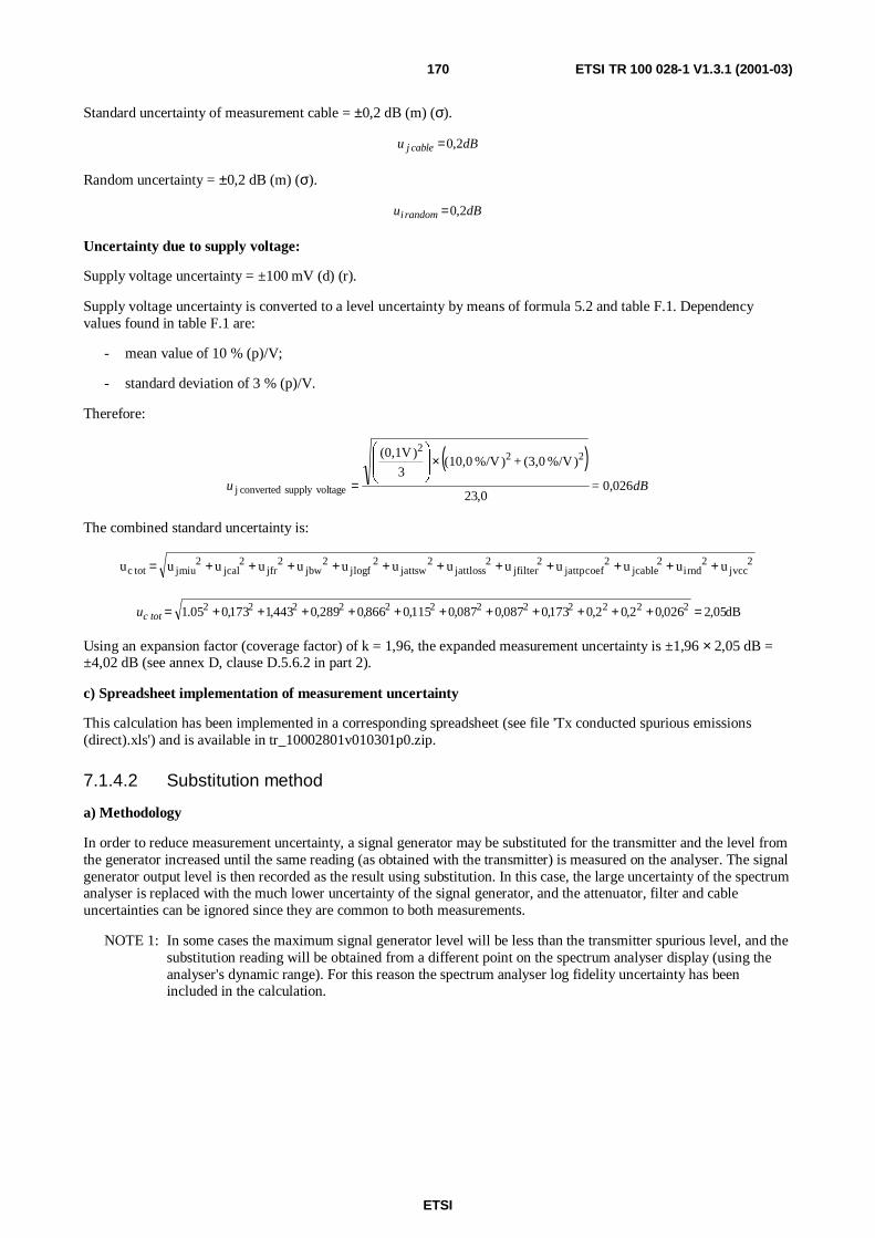
ETSI
ETSI TR 100 028-1 V1.3.1 (2001-03)170
Standard uncertainty of measurement cable = ±0,2 dB (m) (σ).
dBu cablej 2,0=
Random uncertainty = ±0,2 dB (m) (σ).
dBu randomi 2,0=
Uncertainty due to supply voltage:
Supply voltage uncertainty = ±100 mV (d) (r).
Supply voltage uncertainty is converted to a level uncertainty by means of formula 5.2 and table F.1. Dependencyvalues found in table F.1 are:
- mean value of 10 % (p)/V;
- standard deviation of 3 % (p)/V.
Therefore:
( )dB=u 026,0
0,23
)%/V(3,0+)%/V(10,03
)(0,1V 222
voltagesupplyconvertedj
×
=
The combined standard uncertainty is:
2vccj
2rndi
2cablej
2coefpattj
2filterj
2lossattj
2swattj
2flogj
2bwj
2frj
2calj
2miujtotc uuuuuuuuuuuuu +++++++++++=
dB05,2026,02,02,0173,0087,0087,0115,0866,0289,0443,1173,005.1 222222222222 =+++++++++++=c totu
Using an expansion factor (coverage factor) of k = 1,96, the expanded measurement uncertainty is ±1,96 × 2,05 dB =±4,02 dB (see annex D, clause D.5.6.2 in part 2).
c) Spreadsheet implementation of measurement uncertainty
This calculation has been implemented in a corresponding spreadsheet (see file 'Tx conducted spurious emissions(direct).xls') and is available in tr_10002801v010301p0.zip.
7.1.4.2 Substitution method
a) Methodology
In order to reduce measurement uncertainty, a signal generator may be substituted for the transmitter and the level fromthe generator increased until the same reading (as obtained with the transmitter) is measured on the analyser. The signalgenerator output level is then recorded as the result using substitution. In this case, the large uncertainty of the spectrumanalyser is replaced with the much lower uncertainty of the signal generator, and the attenuator, filter and cableuncertainties can be ignored since they are common to both measurements.
NOTE 1: In some cases the maximum signal generator level will be less than the transmitter spurious level, and thesubstitution reading will be obtained from a different point on the spectrum analyser display (using theanalyser's dynamic range). For this reason the spectrum analyser log fidelity uncertainty has beenincluded in the calculation.

ETSI
ETSI TR 100 028-1 V1.3.1 (2001-03)171
cable
alternative cable positionwhen substituting
Spectrum analyserFilter30dB powerattenuator
Signalgenerator
Transmitterundertest
Figure 48b: Conducted spurious emissions measurement configuration (substitution method)
b) Measurement uncertainty: Substitution method
Mismatch uncertainty:
The 30 dB attenuator is large enough to provide good isolation between the transmitter (or signal generator) and thefilter. Thus the only mismatch uncertainty of interest is at the input to the attenuator. The rest cancel due to substitution:
- transmitter reflection coefficient is 0,7 (from table F1);
- measurement cable reflection coefficients are 0,2 (m);
- attenuator input reflection coefficient is 0,1 (d);
- signal generator output reflection coefficient is 0,35 (d).
For the calculation of mismatch, cable attenuation is assumed to be 0,00 dB (x 1 linear).
)(%899,92
%1002,07,0: vu cabletoTxmismatchj =××=
)(%414,12
%1001,02,0: vu attenuatortocablemismatchj =××=
)(%950,42
%100)0,1(1,07,0 2
: vu attenuatortoTxmismatchj =×××=
)(%950,42
%1002,035,0: vu cabletogensigmismatchj =××=
)(%475,22
%100)0,1(1,035,0 2
: vu attenuatortogensigmismatchj =×××=
The combined standard uncertainty for mismatch is:
dBu mismatchc 083,15,11
475,2950,4950,4414,1899,9 22222
=++++
=
Uncertainty when making the measurement:
Substitution signal generator level uncertainty is ±1 dB (d) (r).
0,577dB3
0,1 =±=levelgensigju
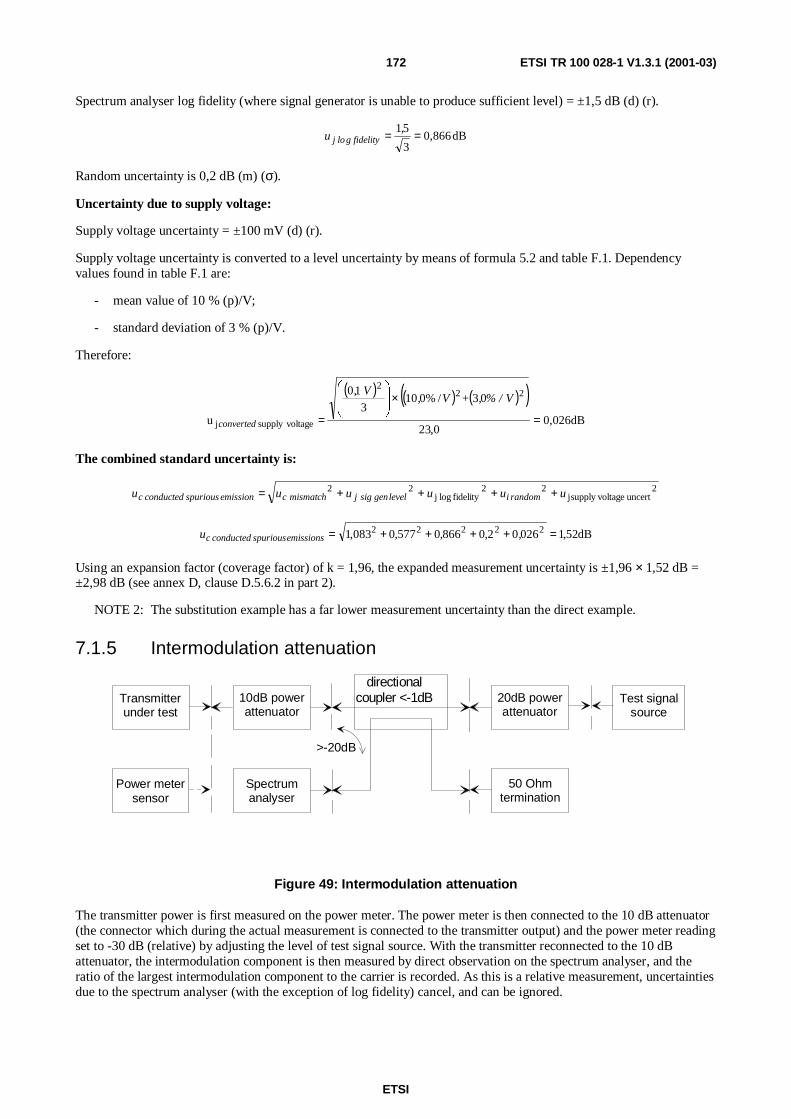
ETSI
ETSI TR 100 028-1 V1.3.1 (2001-03)172
Spectrum analyser log fidelity (where signal generator is unable to produce sufficient level) = ±1,5 dB (d) (r).
dB0,8663
51 == ,u g fidelityj lo
Random uncertainty is 0,2 dB (m) (σ).
Uncertainty due to supply voltage:
Supply voltage uncertainty = ±100 mV (d) (r).
Supply voltage uncertainty is converted to a level uncertainty by means of formula 5.2 and table F.1. Dependencyvalues found in table F.1 are:
- mean value of 10 % (p)/V;
- standard deviation of 3 % (p)/V.
Therefore:
( ) ( ) ( )( )0,026dB
0,23
03/%0103
10
u
222
voltagesupplyj =
×
=
% / V,+V,V,
converted
The combined standard uncertainty is:
2uncertvoltagesupplyj
22fidelitylogj
22 uuuuuu randomilevelgensigjmismatchcemissionspuriousconductedc ++++=
dB52,102602,0866,0577,0083,1 22222 =++++= ,u emissionsspuriousconductedc
Using an expansion factor (coverage factor) of k = 1,96, the expanded measurement uncertainty is ±1,96 × 1,52 dB =±2,98 dB (see annex D, clause D.5.6.2 in part 2).
NOTE 2: The substitution example has a far lower measurement uncertainty than the direct example.
7.1.5 Intermodulation attenuation
Test signalsource
10dB powerattenuator
Transmitterunder test
directionalcoupler <-1dB 20dB power
attenuator
50 Ohmtermination
Power metersensor
Spectrumanalyser
>-20dB
Figure 49: Intermodulation attenuation
The transmitter power is first measured on the power meter. The power meter is then connected to the 10 dB attenuator(the connector which during the actual measurement is connected to the transmitter output) and the power meter readingset to -30 dB (relative) by adjusting the level of test signal source. With the transmitter reconnected to the 10 dBattenuator, the intermodulation component is then measured by direct observation on the spectrum analyser, and theratio of the largest intermodulation component to the carrier is recorded. As this is a relative measurement, uncertaintiesdue to the spectrum analyser (with the exception of log fidelity) cancel, and can be ignored.

ETSI
ETSI TR 100 028-1 V1.3.1 (2001-03)173
b) Measurement uncertainty:
Uncertainty when measuring the transmitter level and setting the level of the test signal source to -30 dB relative:
NOTE: The power meter is only used to set the test signal source to -30 dB relative to the transmitter level soonly range change and linearity need to be considered.
Power meter linearity = ±0,5 % (p) (d) (r).
dB,0130233
5,0u linmeterj =
×=
Power meter range change error (one change) = ±0,5 % (p) (d) (r).
dB,0130233
5,0u errorchangerangej =
×=
dB,0180013,0013,0u 22levelsignaltestc =+=
Mismatch uncertainty when measuring the transmitter level and setting the level of the test signal source to-30 dB relative:
- transmitter reflection coefficient is 0,5 (table F.1);
- power sensor reflection coefficient is 0,07 (d);
- attenuator reflection coefficients are 0,1 (d) (both attenuators);
- directional coupler reflection coefficients are 0,05 (d).
For the following mismatch calculations the directional coupler loss is assumed to be 0 dB (x1 linear). The isolatingeffect of the10 dB attenuator is however taken into consideration (multiplication by 0,316 in linear terms).
Only the reflection coefficients of the transmitter, 10 dB attenuator, the directional coupler and the 20 dB attenuator aretaken into account, the test signal source is ignored due to isolation. It is assumed that the spectrum analyser isconnected during the power measurement with the same cable and the same attenuator setting as during themeasurement. Therefore the mismatch uncertainties at this point cancel.
)(02502
1003160050070 2v%,
%,,,u couplerirectionalnsor and d: power sej mismatch =×××=
)(04902
1001316010070 22
20 v%,%,,,
u atordB attenunsor and: power sej mismatch =××××=
)(5252049,0025,0495,0475,2 2222 v%,u signaltestg: measurinc mismatch =+++=
Mismatch uncertainty with the transmitter reconnected to the 10dB attenuator:
Only the reflection coefficients of the transmitter, 10 dB attenuator, the directional coupler and the 20 dB attenuator aretaken into account, the test signal source is ignored due to isolation:
- transmitter reflection coefficient is 0,5 (table F1);
- attenuator reflection coefficients are 0,1 (d);
- directional coupler reflection coefficients are 0,05 (d).
For the following mismatch calculations the directional coupler loss is assumed to be 0 dB (x1 linear). The isolatingeffect of the10 dB attenuator is however taken into consideration (multiplication with 0,316 in linear terms).
)(536,32
1001050attenuator10dBandertransmitt:mismatchj v%
%,,u =××=

ETSI
ETSI TR 100 028-1 V1.3.1 (2001-03)174
)(17702
100316005050 2v%,
%,,,u couplerrectionalter and di: transmitj mismatch =×××=
)(35302
100131601050 22
20 v%,%,,,
u tordB attenuater and: transmitj mismatch =××××=
)(558,335301770536,3 222connectedsignaltest:mismatchc v%,,u =++=
Combined mismatch uncertainties:
dBu 379,05,11
558,3525,2 22
hmismatcc =+
=
Combined uncertainty of the test signal:
dB,3790379,0018,0u 22signaltestc =+=
Spectrum analyser log fidelity = ±1,5 dB (d) (r):
dBu 866,03
5,1fidelitylogj ==
One of the intermodulation products has a 2nd order dependency from the unwanted signal corresponding to 2 dB/dB,therefore the uncertainty of the level of the intermodulation product is doubled (see clause 6.5.5, and annex Dclauses D.3.4.5.2 and D.5).
The combined standard uncertainty for intermodulation attenuation is:
( ) dB151379028660 22 ,,,u ntmeasuremettenuationdulation antermoc i =×+=
Using an expansion factor (coverage factor) of k = 1,96, the expanded measurement uncertainty is ±1,96 × 1,15 dB =±2,25 dB (see annex D, clause D.5.6.2 in part 2).
7.1.6 Attack time
7.1.6.1 Frequency behaviour (attack)
a) Methodology
Frequency behaviour (attack) is the time elapsed between switching on the transmitter and the moment when the carrierfrequency is within defined limits. Transmitter output frequency variation as a function of time during this period ismeasured by means of a test discriminator providing vertical deflection to a storage oscilloscope (see figure 50).

ETSI
ETSI TR 100 028-1 V1.3.1 (2001-03)175
Triggerdevice
Transmitterundertest trigger
cable
Storageoscilloscope
Referencesignalgenerator
Yinput
Txon/off
Testdiscriminator
cablePowerattenuator
Figure 50: Transmitter frequency/time measurement configuration (attack and release)
With the oscilloscope time base set to 'repetitive' at an appropriate sweep rate, the oscilloscope display graticule iscalibrated by means of the signal generator, to provide vertical reference points corresponding to the specificationfrequency limits or mask e.g. ± one channel. The oscilloscope is then set to "single sweep" in preparation for themeasurement.
When the trigger device is operated, it initiates the oscilloscope sweep and simultaneously switches on the transmitter.Any variation in transmitter output frequency will appear at the discriminator output as a varying DC voltage which willbe recorded on the oscilloscope display as a plot of frequency against time.
b) Measurement uncertainty:
- signal generator frequency uncertainty is ±10 Hz (d) (r);
- calibration uncertainty of discriminator (including the storage oscilloscope) is ±100 Hz (r);
- DC drift of discriminator is equivalent to ±100 Hz (d) (r).
Combined standard uncertainty of the frequency measurement:
Hz81,9=3
10100100 222 ))Hz+()Hz+()Hz((=u enty measuremj frequenc
Frequency uncertainty is converted to time uncertainty by means of formula 5.2 and table F.1. Dependency valuesfound in table F.1 are:
- mean value of 1,0 ms/kHz;
- standard deviation of 0,3 ms/kHz.
Therefore:
ms0,086=))ms/kHz(0,3+)ms/kHz((1,0)kHz(0,0819=u 222timej ×
Random uncertainty is 0,5 ms (m) (c) (σ).
Oscilloscope timing uncertainty is ±1,0 ms (d) (r).
Trigger moment uncertainty is ±1,0 ms (d) (r).
The combined standard uncertainty:
ms0,961=3
)ms(1+)ms(1+)ms(0,5+)ms(0,086u
2222
behaviourfrequencyc
=

ETSI
ETSI TR 100 028-1 V1.3.1 (2001-03)176
Using an expansion factor (coverage factor) of k = 1,96, the expanded measurement uncertainty is ±1,96 × 0,961 ms =±1,9 ms (see annex D, clause D.5.6.2 in part 2).
7.1.6.2 Power behaviour (attack)
a) Methodology
Power behaviour (attack) is the time elapsed between switching on the transmitter and the moment when the transmitteroutput power level is within defined limits i.e. a percentage of full power. Transmitter output power variation as afunction of time during this period is measured on a spectrum analyser set to zero span mode (see figure 51).
Triggerdevice
Transmitterundertest
trigger
cable
Spectrumanalyser
RFinputTxon/off
cablePowerattenuator
Figure 51: Transmitter power level/time measurement configuration (attack and release)
With the spectrum analyser time base set to "repetitive" at an appropriate sweep rate, the transmitter is switched on andthe analyser sensitivity adjusted until the measured signal coincides with the reference level. The analyser is then set to"single shot", and the transmitter switched off in preparation for the measurement.
When the trigger device is operated, this simultaneously initiates the spectrum analyser sweep and switches on thetransmitter. Any variation in transmitter output power level will be recorded on the spectrum analyser display as a plotof output power level against time.
b) Measurement uncertainty:
Spectrum analyser log fidelity ±0,4 dB (d) (r).
dB0,2313
40log ==
,u fidelityj
The power level difference uncertainty is then converted to time uncertainty by means of formula 5.2 and table F.1.Dependency values found in table F.1 are:
- mean value of 0,3 ms/%;
- standard deviation of 0,1 ms/%.
Therefore:
( ) ( ) ( )( ) ms0,84010305112310 222 =+××= ms / %,ms / %,,,u j time
Random uncertainty is 0,5 ms (m) (c) (σ).
Oscilloscope timing uncertainty is ±1,0 ms (d) (r).
Trigger moment uncertainty is ±1,0 ms (d) (r).
The combined standard uncertainty:
ms1,274=3
11508400
2222 )
)ms+()ms(+()ms,+()ms,(u ry behaviouc frequenc =

ETSI
ETSI TR 100 028-1 V1.3.1 (2001-03)177
Using an expansion factor (coverage factor) of k = 1,96, the expanded measurement uncertainty is ±1,96 × 1,274 ms =±2,5 ms (see annex D, clause D.5.6.2 in part 2).
7.1.7 Release time
7.1.7.1 Frequency behaviour (release)
The only difference between this measurement and the measurement for attack in clause 7.1.6.1 is that in this case themeasurement is to determine the time elapsed between switching off the transmitter and the moment when the carrierfrequency falls outside defined limits. Measurement uncertainty for release is therefore the same as for attack.
7.1.7.2 Power behaviour (release)
The only difference between this measurement and the measurement for attack in clause 7.1.6.2 is that in this case themeasurement is to determine the time elapsed between switching off the transmitter and the moment when the carrierpower is within defined limits. Measurement uncertainty for release is therefore the same as for attack.
7.1.8 Transient behaviour of the transmitter
Transient behaviour of the transmitter is the period of transient frequency/power behaviour immediately following theswitching on or off of the transmitter.
7.1.8.1 Transient frequency behaviour
a) Methodology
Transient frequency behaviour is the frequency error of the transmitter during switch on and switch off transients.Transmitter frequency error as a function of time during this period is measured by means of a test discriminatorproviding vertical deflection to a storage oscilloscope (see figure 52a).
Triggerdevice
Transmitterundertest trigger
cable
Storageoscilloscope
Referencesignalgenerator
Yinput
Txon/off
Testdiscriminator
cablePowerattenuator
Figure 52a: Transmitter frequency/time measurement configuration (attack and release)
With the transmitter switched off, the oscilloscope time base is set to 'repetitive' at an appropriate sweep rate. Theoscilloscope display graticule is then calibrated by means of the signal generator, to provide vertical reference pointscorresponding to the specification frequency limits or mask e.g. ± one channel. When this has been accomplished, thetrigger selector is set to 'single sweep' and the transmitter set to on or off depending upon which transient condition is tobe measured.
When the trigger device is operated, this simultaneously initiates the oscilloscope sweep and switches the transmitter onor off according to the measurement. Any variation in transmitter output frequency will appear at the discriminatoroutput as a varying DC voltage which will be recorded on the oscilloscope display as a plot of frequency against time.
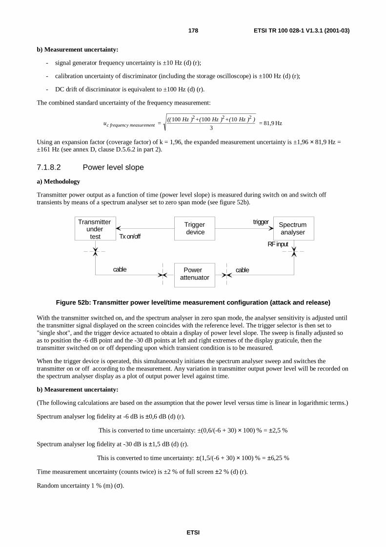
ETSI
ETSI TR 100 028-1 V1.3.1 (2001-03)178
b) Measurement uncertainty:
- signal generator frequency uncertainty is ±10 Hz (d) (r);
- calibration uncertainty of discriminator (including the storage oscilloscope) is ±100 Hz (d) (r);
- DC drift of discriminator is equivalent to ±100 Hz (d) (r).
The combined standard uncertainty of the frequency measurement:
Hz81,9=3
10100100 222 ))Hz+()Hz+()Hz((=u enty measuremc frequenc
Using an expansion factor (coverage factor) of k = 1,96, the expanded measurement uncertainty is ±1,96 × 81,9 Hz =±161 Hz (see annex D, clause D.5.6.2 in part 2).
7.1.8.2 Power level slope
a) Methodology
Transmitter power output as a function of time (power level slope) is measured during switch on and switch offtransients by means of a spectrum analyser set to zero span mode (see figure 52b).
Triggerdevice
Transmitterundertest
trigger
cable
Spectrumanalyser
RFinputTxon/off
cablePowerattenuator
Figure 52b: Transmitter power level/time measurement configuration (attack and release)
With the transmitter switched on, and the spectrum analyser in zero span mode, the analyser sensitivity is adjusted untilthe transmitter signal displayed on the screen coincides with the reference level. The trigger selector is then set to"single shot", and the trigger device actuated to obtain a display of power level slope. The sweep is finally adjusted soas to position the -6 dB point and the -30 dB points at left and right extremes of the display graticule, then thetransmitter switched on or off depending upon which transient condition is to be measured.
When the trigger device is operated, this simultaneously initiates the spectrum analyser sweep and switches thetransmitter on or off according to the measurement. Any variation in transmitter output power level will be recorded onthe spectrum analyser display as a plot of output power level against time.
b) Measurement uncertainty:
(The following calculations are based on the assumption that the power level versus time is linear in logarithmic terms.)
Spectrum analyser log fidelity at -6 dB is ±0,6 dB (d) (r).
This is converted to time uncertainty: ±(0,6/(-6 + 30) × 100) % = ±2,5 %
Spectrum analyser log fidelity at -30 dB is ±1,5 dB (d) (r).
This is converted to time uncertainty: ±(1,5/(-6 + 30) × 100) % = ±6,25 %
Time measurement uncertainty (counts twice) is ±2 % of full screen ±2 % (d) (r).
Random uncertainty 1 % (m) (σ).

ETSI
ETSI TR 100 028-1 V1.3.1 (2001-03)179
The combined standard uncertainty is:
%,=%+%+%+%,%,
u vel slopec power le 3340,13
0,20,225652 22222 +=
Using an expansion factor (coverage factor) of k = 1,96, the expanded measurement uncertainty is ±1,96 × 4,33 % =±8,5 % (see annex D, clause D.5.6.2 in part 2).
7.1.9 Frequency deviation
7.1.9.1 Maximum permissible frequency deviation
a) Methodology
The AF signal from the audio frequency oscillator is applied to the modulation input of the transmitter under test at alevel 20 dB above the level of normal test modulation (see figure 53).
cable cablePowerattenuator
Transmitterundertest
ModulatingAF oscillator
Deviationmeter
Figure 53: Maximum permissible frequency deviation measurement configuration
The RF output from the transmitter under test is applied to a deviation meter through a power attenuator. The maximumdeviation is measured as 4,0 kHz.
b) Measurement uncertainty
As the modulating signal level is 20 dB above that required for normal test modulation, it is assumed that the AF leveluncertainty of the modulating AF oscillator has no influence.
Deviation uncertainty is ±1 % ±1 digit (f) (d) (r).
±1 digit is 10 Hz which is calculated as (10/4000) × 100 % = ±0,25 %.
Residual modulation is ±20 Hz (f) (d) (r) which is converted to a percentage of the measured deviation (4 kHz):(20/4 000) × 100 % = ±0,5 %
NOTE: The random contribution is deemed to be negligible and has therefore been ignored.
The combined standard uncertainty for maximum permissible frequency deviation is:
%0,66=3
)%(0,5+)%(0,25+)%(1,0=u
222
totalj
Using an expansion factor (coverage factor) of k = 1,96, the expanded measurement uncertainty is ±1,96 × 0,66 % =±1,3 % (see annex D, clause D.5.6.2 in part 2).
c) Spreadsheet implementation of measurement uncertainty
This calculation has been implemented in a corresponding spreadsheet (see file "Maximum permissible frequencydeviation.xls") and is available in tr_10002801v010301p0.zip.

ETSI
ETSI TR 100 028-1 V1.3.1 (2001-03)180
7.1.9.2 Response of the transmitter to modulation frequencies above 3 kHz
a) Methodology
The AF signal from the audio frequency oscillator is applied to the modulation input of the transmitter under test at thespecified level (see figure 54).
cable cablePowerattenuator
Deviationmeter
Low noisesignal generator
Audioanalyser
ModulatingAF oscillator
Transmitterundertest
Figure 54: Measurement configuration for modulation frequencies above 3 kHz
The RF output from the transmitter under test is applied to a deviation meter through a power attenuator. Thedemodulated signal is then applied to the audio analyser. A low noise signal generator is used as the local oscillator forthe deviation meter for demodulating signals with modulation frequencies above 3 kHz, to improve the noise behaviour.The result is corrected for AF gain and AF filter shaping. It is assumed that the measurement is conducted sufficientlyabove the measuring system noise level.
b) Measurement uncertainty:
(As a low noise signal generator is used for the deviation meter local oscillator, it is assumed that residual deviation isinsignificant and has no influence on the measurement).
AF oscillator level uncertainty = ±0,70 % (v) (d) (r).
Deviation meter demodulator uncertainty = ±1,0 % (v) (d) (r).
Deviation meter AF gain uncertainty = ±2,0 % (v) (d) (r).
Audio analyser AC voltmeter uncertainty = ±4,0 % (v) (d) (r).
The combined standard uncertainty is then calculated:
2,68%=3
020401700 2222 )%,+()%,+()%,+()%,(=u j
The combined standard uncertainty is converted to dB: 2,68 %/11,5 = 0,233 dB.
Using an expansion factor (coverage factor) of k = 1,96, the expanded measurement uncertainty is ±1,96 × 0,233 dB =±0,46 dB (see annex D, clause D.5.6.2 in part 2).
c) Spreadsheet implementation of measurement uncertainty
This calculation has been implemented in a corresponding spreadsheet (see file "Response to mod freqs above3kHz.xls") and is available in tr_10002801v010301p0.zip.
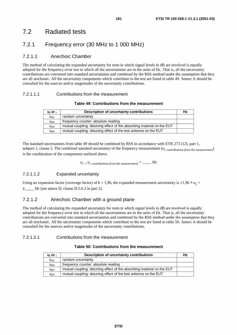
ETSI
ETSI TR 100 028-1 V1.3.1 (2001-03)181
7.2 Radiated tests
7.2.1 Frequency error (30 MHz to 1 000 MHz)
7.2.1.1 Anechoic Chamber
The method of calculating the expanded uncertainty for tests in which signal levels in dB are involved is equallyadopted for the frequency error test in which all the uncertainties are in the units of Hz. That is, all the uncertaintycontributions are converted into standard uncertainties and combined by the RSS method under the assumption that theyare all stochastic. All the uncertainty components which contribute to the test are listed in table 49. Annex A should beconsulted for the sources and/or magnitudes of the uncertainty contributions.
7.2.1.1.1 Contributions from the measurement
Table 49: Contributions from the measurement
uj or i Description of uncertainty contributions Hzui01 random uncertaintyuj56 frequency counter: absolute readinguj05 mutual coupling: detuning effect of the absorbing material on the EUTuj09 mutual coupling: detuning effect of the test antenna on the EUT
The standard uncertainties from table 49 should be combined by RSS in accordance with ETR 273 [12], part 1,subpart 1, clause 5. The combined standard uncertainty of the frequency measurement (uc contributions from the measurement)
is the combination of the components outlined above.
uc = uc contributions from the measurement = __,__ Hz
7.2.1.1.2 Expanded uncertainty
Using an expansion factor (coverage factor) of k = 1,96, the expanded measurement uncertainty is ±1,96 × uc =
±__,__ Hz (see annex D, clause D.5.6.2 in part 2).
7.2.1.2 Anechoic Chamber with a ground plane
The method of calculating the expanded uncertainty for tests in which signal levels in dB are involved is equallyadopted for the frequency error test in which all the uncertainties are in the units of Hz. That is, all the uncertaintycontributions are converted into standard uncertainties and combined by the RSS method under the assumption that theyare all stochastic. All the uncertainty components which contribute to the test are listed in table 50. Annex A should beconsulted for the sources and/or magnitudes of the uncertainty contributions.
7.2.1.2.1 Contributions from the measurement
Table 50: Contributions from the measurement
uj or i Description of uncertainty contributions Hzui01 random uncertaintyuj56 frequency counter: absolute readinguj05 mutual coupling: detuning effect of the absorbing material on the EUTuj09 mutual coupling: detuning effect of the test antenna on the EUT

ETSI
ETSI TR 100 028-1 V1.3.1 (2001-03)182
7.2.1.2.2 Expanded uncertainty
The standard uncertainties from table 50 should be combined by RSS in accordance with ETR 273 [12], part 1,subpart 1, clause 5. The combined standard uncertainty of the frequency measurement (uc contributions from the measurement)
is the combination of the components outlined above.
uc = uc contributions from the measurement = __,__ Hz
Using an expansion factor (coverage factor) of k = 1,96, the expanded measurement uncertainty is ±1,96 × uc =
±__,__ Hz (see annex D, clause D.5.6.2 in part 2).
7.2.1.3 Open Area Test Site
The method of calculating the expanded uncertainty for tests in which signal levels in dB are involved is equallyadopted for the frequency error test in which all the uncertainties are in the units of Hz. That is, all the uncertaintycontributions are converted into standard uncertainties and combined by the RSS method under the assumption that theyare all stochastic. All the uncertainty components which contribute to the test are listed in table 51. Annex A should beconsulted for the sources and/or magnitudes of the uncertainty contributions.
7.2.1.3.1 Contributions from the measurement
Table 51: Contributions from the measurement
uj or i Description of uncertainty contributions Hzui01 random uncertaintyuj09 mutual coupling: detuning effect of the test antenna on the EUTuj56 frequency counter: absolute reading
7.2.1.3.2 Expanded uncertainty
The standard uncertainties from table 51 should be combined by RSS in accordance with ETR 273 [12], part 1,subpart 1, clause 5. The combined standard uncertainty of the frequency measurement (uc contributions from the measurement)is the combination of the components outlined above.
uc = uc contributions from the measurement = __,__ Hz
Using an expansion factor (coverage factor) of k = 1,96, the expanded measurement uncertainty is ±1,96 × uc =
±__,__ Hz (see annex D, clause D.5.6.2 in part 2).
7.2.1.4 Stripline
This test is not usually performed in a Stripline and is therefore not considered here.
7.2.1.5 Test fixture
The method of calculating the expanded uncertainty for tests in which signal levels in dB are involved is equallyadopted for the frequency error test in which all the uncertainties are in the units of Hz. That is, all the uncertaintycontributions are converted into standard uncertainties and combined by the RSS method under the assumption that theyare all stochastic. All the uncertainty components which contribute to the test are listed in table 52. Annex A should beconsulted for the sources and/or magnitudes of the uncertainty contributions.
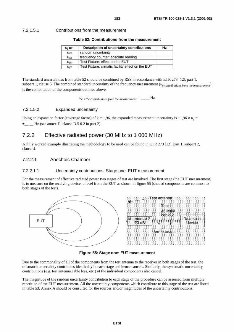
ETSI
ETSI TR 100 028-1 V1.3.1 (2001-03)183
7.2.1.5.1 Contributions from the measurement
Table 52: Contributions from the measurement
uj or i Description of uncertainty contributions Hzui01 random uncertaintyuj56 frequency counter: absolute readinguj60 Test Fixture: effect on the EUTuj61 Test Fixture: climatic facility effect on the EUT
The standard uncertainties from table 52 should be combined by RSS in accordance with ETR 273 [12], part 1,subpart 1, clause 5. The combined standard uncertainty of the frequency measurement (uc contributions from the measurement)is the combination of the components outlined above.
uc = uc contributions from the measurement = __,__ Hz
7.2.1.5.2 Expanded uncertainty
Using an expansion factor (coverage factor) of k = 1,96, the expanded measurement uncertainty is ±1,96 × uc =
±__,__ Hz (see annex D, clause D.5.6.2 in part 2).
7.2.2 Effective radiated power (30 MHz to 1 000 MHz)
A fully worked example illustrating the methodology to be used can be found in ETR 273 [12], part 1, subpart 2,clause 4.
7.2.2.1 Anechoic Chamber
7.2.2.1.1 Uncertainty contributions: Stage one: EUT measurement
For the measurement of effective radiated power two stages of test are involved. The first stage (the EUT measurement)is to measure on the receiving device, a level from the EUT as shown in figure 55 (shaded components are common toboth stages of the test).
Testantennacable 2
Test antenna
ferrite beads
Attenuator 210 dB
ReceivingdeviceEUT
Figure 55: Stage one: EUT measurement
Due to the commonality of all of the components from the test antenna to the receiver in both stages of the test, themismatch uncertainty contributes identically in each stage and hence cancels. Similarly, the systematic uncertaintycontributions (e.g. test antenna cable loss, etc.) of the individual components also cancel.
The magnitude of the random uncertainty contribution to each stage of the procedure can be assessed from multiplerepetition of the EUT measurement. All the uncertainty components which contribute to this stage of the test are listedin table 53. Annex A should be consulted for the sources and/or magnitudes of the uncertainty contributions.

ETSI
ETSI TR 100 028-1 V1.3.1 (2001-03)184
Table 53: Contributions from the EUT measurement
uj or i Description of uncertainty contributions dBuj37 mismatch: receiving partuj19 cable factor: test antenna cableuj41 insertion loss: test antenna cable 0,00uj40 insertion loss: test antenna attenuator 0,00uj47 receiving device: absolute leveluj53 EUT: influence of setting the power supply on the ERP of the carrieruj20 position of the phase centre: within the EUT volumeuj21 positioning of the phase centre: within the EUT over the axis of rotation of the turntableuj50 EUT: influence of the ambient temperature on the ERP of the carrieruj16 range length 0,00uj01 reflectivity of absorbing material: EUT to the test antenna 0,00uj45 antenna: gain of the test antenna 0,00uj46 antenna: tuning of the test antenna 0,00uj55 EUT: mutual coupling to the power leadsuj08 mutual coupling: amplitude effect of the test antenna on the EUTuj04 mutual coupling: EUT to its images in the absorbing materialuj06 mutual coupling: test antenna to its images in the absorbing materialui01 random uncertainty
The standard uncertainties from table 53 should be combined by RSS in accordance with ETR 273 [12], part 1,subpart 1, clause 5. This gives the combined standard uncertainty (uc contribution from the EUT measurement) for the EUT
measurement in dB.
7.2.2.1.2 Uncertainty contributions: Stage two: Substitution
The second stage (the substitution) involves replacing the EUT with a substitution antenna and signal source as shownin figure 56 and adjusting the output level of the signal generator until the same level as in stage one is achieved on thereceiving device.
Testantennacable 2
Test antenna
ferrite beads
Attenuator 210 dB
Receivingdevice
cable 1
ferrite beads
Attenuator 110 dB
Signalgenerator
Figure 56: Stage two: Substitution measurement
All the uncertainty components which contribute to this stage of the test are listed in table 54. Annex A should beconsulted for the sources and/or magnitudes of the uncertainty contributions.

ETSI
ETSI TR 100 028-1 V1.3.1 (2001-03)185
Table 54: Contributions from the substitution
uj or i Description of uncertainty contributions dBuj36 mismatch: transmitting partuj37 mismatch: receiving partuj38 signal generator: absolute output leveluj39 signal generator: output level stabilityuj19 cable factor: substitution antenna cableuj19 cable factor: test antenna cableuj41 insertion loss: substitution antenna cableuj41 insertion loss: test antenna cable 0,00uj40 insertion loss: substitution antenna attenuatoruj40 insertion loss: test antenna attenuator 0,00uj47 receiving device: absolute level 0,00uj16 range length 0,00uj02 reflectivity of absorbing material: substitution antenna to the test antenna 0,00uj45 antenna: gain of the substitution antenna 0,50uj45 antenna: gain of the test antenna 0,00uj46 antenna: tuning of the test antenna 0,00uj22 position of the phase centre: substitution antennauj06 mutual coupling: substitution antenna to its images in the absorbing materialuj06 mutual coupling: test antenna to its images in the absorbing material 0,50uj11 mutual coupling: substitution antenna to the test antenna 0,00uj12 mutual coupling: interpolation of mutual coupling and mismatch loss correction factors 0,00ui01 random uncertainty
The standard uncertainties from table 54 should be combined by RSS in accordance with ETR 273 [12], part 1,subpart 1, clause 5. This gives the combined standard uncertainty (uc contributions from the substitution) for the substitutionmeasurement in dB.
7.2.2.1.3 Expanded uncertainty
The combined standard uncertainty of the effective radiated power measurement is the RSS combination of thecomponents outlined in clauses 7.2.2.1.1 and 7.2.2.1.2. The components to be combined are uc contribution from the EUT
measurement and uc contribution from the substitution.
dB____,22 =+= onsubstitutithefromoncontributictmeasuremenEUTthefromoncontributicc uuu
Using an expansion factor (coverage factor) of k = 1,96, the expanded measurement uncertainty is ±1,96 × uc =
±__,__ dB (see annex D, clause D.5.6.2 in part 2).

ETSI
ETSI TR 100 028-1 V1.3.1 (2001-03)186
7.2.2.2 Anechoic Chamber with a ground plane
7.2.2.2.1 Uncertainty contributions: Stage one: EUT measurement
For the measurement of effective radiated power two stages of test are involved. The first stage (the EUT measurement)is to measure on the receiving device, a level from the EUT as shown in figure 57 (shaded components are common toboth stages of the test).
Testantennacable 2
Test antenna
ferrite beads
EUT Attenuator 210 dB
Receivingdevice
Ground plane
Figure 57: Stage one: EUT measurement
Due to the commonality of all of the components from the test antenna to the receiver in both stages of the test, themismatch uncertainty contributes identically to both stages and hence cancels. Similarly, the systematic uncertaintycontributions (e.g. test antenna cable loss, etc.) of the individual components also cancel.
The magnitude of the random uncertainty contribution to this stage of the procedure can be assessed from multiplerepetition of the EUT measurement. All the uncertainty components which contribute to this stage of the test are listedin table 55. Annex A should be consulted for the sources and/or magnitudes of the uncertainty contributions.
Table 55: Contributions from the EUT measurement
uj or i Description of uncertainty contributions dBuj37 mismatch: receiving partuj19 cable factor: test antenna cable 0,00uj41 insertion loss: test antenna cable 0,00uj40 insertion loss: test antenna attenuator 0,00uj47 receiving device: absolute level 0,00uj53 EUT: influence of setting the power supply on the ERP of the carrieruj20 position of the phase centre: within the EUT volumeuj21 positioning of the phase centre: within the EUT over the axis of rotation of the turntableuj50 EUT: influence of the ambient temperature on the ERP of the carrieruj16 range lengthuj01 reflectivity of absorbing material: EUT to the test antennauj45 antenna: gain of the test antenna 0,00uj46 antenna: tuning of the test antenna 0,00uj17 correction: off boresight angle in the elevation plane 0,00uj55 EUT: mutual coupling to the power leadsuj08 mutual coupling: amplitude effect of the test antenna on the EUTuj04 mutual coupling: EUT to its images in the absorbing materialuj13 mutual coupling: EUT to its image in the ground planeuj06 mutual coupling: test antenna to its images in the absorbing materialuj14 mutual coupling: test antenna to its image in the ground planeui01 random uncertainty
The standard uncertainties from table 55 should be combined by RSS in accordance with ETR 273 [12], part 1,subpart 1, clause 5. This gives the combined standard uncertainty (uc contribution from the EUT measurement) for the EUTmeasurement in dB.

ETSI
ETSI TR 100 028-1 V1.3.1 (2001-03)187
7.2.2.2.2 Uncertainty contributions: Stage two: Substitution measurement
The second stage (the substitution) involves replacing the EUT with a substitution antenna and signal source as shownin figure 58 and adjusting the output level of the signal generator until the same level as in stage one is achieved on thereceiving device.
Ground plane
Testantennacable 1
Test antenna
ferrite beads
Attenuator 110 dB
Receivingdevice
cable 1
ferrite beads
Attenuator 110 dB
Signalgenerator
Figure 58: Stage two: Substitution measurement
All the uncertainty components which contribute to this stage of the test are listed in table 56. Annex A should beconsulted for the sources and/or magnitudes of the uncertainty contributions.
Table 56: Contributions from the substitution
uj or i Description of uncertainty contributions dBuj36 mismatch: transmitting partuj37 mismatch: receiving partuj38 signal generator: absolute output leveluj39 signal generator: output level stabilityuj19 cable factor: substitution antenna cableuj19 cable factor: test antenna cableuj41 insertion loss: substitution antenna cableuj41 insertion loss: test antenna cable 0,00uj40 insertion loss: substitution antenna attenuatoruj40 insertion loss: test antenna attenuator 0,00uj47 receiving device: absolute level 0,00uj16 range length 0,00uj18 correction: measurement distanceuj02 reflectivity of absorbing material: substitution antenna to the test antennauj45 antenna: gain of substitution antennauj45 antenna: gain of the test antenna 0,00uj46 antenna: tuning of the substitution antennauj46 antenna: tuning of the test antenna 0,00uj22 position of the phase centre: substitution antennauj17 correction: off boresight angle in the elevation planeuj06 mutual coupling: substitution antenna to its images in the absorbing materialuj06 mutual coupling: test antenna to its images in the absorbing materialuj14 mutual coupling: substitution antenna to its image in the ground planeuj14 mutual coupling: test antenna to its image in the ground planeuj11 mutual coupling: substitution antenna to the test antennauj12 mutual coupling: interpolation of mutual coupling and mismatch loss correction factorsui01 random uncertainty
The standard uncertainties from table 56 should be combined by RSS in accordance with ETR 273 [12], part 1,subpart 1, clause 5. This gives the combined standard uncertainty (uc contributions from the substitution) for the substitutionmeasurement in dB.

ETSI
ETSI TR 100 028-1 V1.3.1 (2001-03)188
7.2.2.2.3 Expanded uncertainty
The combined standard uncertainty of the effective radiated power measurement is the RSS combination of thecomponents outlined in 7.2.4.1 and 7.2.4.2. The components to be combined are uc contribution from the EUT measurement and
uc contribution from the substitution.
dB____,22 =+= onsubstitutithefromoncontributictmeasuremenEUTthefromoncontributicc uuu
Using an expansion factor (coverage factor) of k = 1,96, the expanded measurement uncertainty is ±1,96 × uc =
±__,__ dB (see annex D, clause D.5.6.2 in part 2).
7.2.2.3 Open Area Test Site
7.2.2.3.1 Uncertainty contributions: Stage one: EUT measurement
For the measurement of effective radiated power two stages of test are involved. The first stage (the EUT measurement)is to measure on the receiving device, a level from the EUT as shown in figure 59 (shaded components are common toboth stages of the test).
Testantennacable 2
Test antenna
ferrite beads
EUT Attenuator 210 dB
Receivingdevice
Ground plane
Figure 59: Stage one: EUT measurement
Due to the commonality of all of the components from the test antenna to the receiver in both stages of the test, themismatch uncertainty contributes identically in each stage and hence cancels. Similarly, the systematic uncertaintycontributions (e.g. test antenna cable loss, etc.) of the individual components also cancel.
The magnitude of the random uncertainty contribution to each stage of the procedure can be assessed from multiplerepetition of the EUT measurements. All the uncertainty components which contribute to this stage of the test are listedin table 57. Annex A should be consulted for the sources and/or magnitudes of the uncertainty contributions.

ETSI
ETSI TR 100 028-1 V1.3.1 (2001-03)189
Table 57: Contributions from the EUT measurement
uj or i Description of uncertainty contributions dBuj37 mismatch: receiving partuj19 cable factor: test antenna cable 0,00uj41 insertion loss: test antenna cable 0,00uj40 insertion loss: test antenna attenuator 0,00uj47 receiving device: absolute level 0,00uj53 EUT: influence of setting the power supply on the ERP of the carrieruj20 position of the phase centre: within the EUT volumeuj21 positioning of the phase centre: within the EUT over the axis of rotation of the turntableuj50 EUT: influence of the ambient temperature on the ERP of the carrieruj16 range lengthuj45 antenna: gain of the test antenna 0,00uj46 antenna: tuning of the test antenna 0,00uj17 correction: off boresight angle in the elevation plane 0,00uj55 EUT: mutual coupling to the power leadsuj08 mutual coupling: amplitude effect of the test antenna on the EUTuj13 mutual coupling: EUT to its image in the ground planeuj14 mutual coupling: test antenna to its image in the ground planeui01 random uncertainty
The standard uncertainties from table 57 should be combined by RSS in accordance with ETR 273 [12], part 1,subpart 1, clause 5. This gives the combined standard uncertainty (uc contribution from the EUT measurement) for the EUT
measurement in dB.
7.2.2.3.2 Uncertainty contributions: Stage two: Substitution measurement
The second stage (the substitution) involves replacing the EUT with a substitution antenna and signal source as shownin figure 60 and adjusting the output level of the signal generator until the same level as in stage one is achieved on thereceiving device.
Ground plane
cable 1
ferrite beads
Attenuator 110 dB
Signalgenerator
Testantennacable 2
Test antenna
ferrite beads
Attenuator 210 dB
Receivingdevice
Figure 60: Stage two: Substitution
All the uncertainty components which contribute to this stage of the test are listed in table 58. Annex A should beconsulted for the sources and/or magnitudes of the uncertainty contributions.

ETSI
ETSI TR 100 028-1 V1.3.1 (2001-03)190
Table 58: Contributions from the substitution
uj or i Description of uncertainty contributions dBuj36 mismatch: transmitting partuj37 mismatch: receiving partuj38 signal generator: absolute output leveluj39 signal generator: output level stabilityuj19 cable factor: substitution antenna cableuj19 cable factor: test antenna cableuj41 insertion loss: substitution antenna cableuj41 insertion loss: test antenna cable 0,00uj40 insertion loss: substitution antenna attenuatoruj40 insertion loss: test antenna attenuator 0,00uj47 receiving device: absolute level 0,00uj16 range length 0,00uj18 correction: measurement distanceuj45 antenna: gain of the substitution antennauj45 antenna: gain of the test antenna 0,00uj46 antenna: tuning of the substitution antennauj46 antenna: tuning of the test antenna 0,00uj22 position of the phase centre: substitution antennauj17 correction: off boresight angle in the elevation planeuj14 mutual coupling: substitution antenna to its image in the ground planeuj14 mutual coupling: test antenna to its image in the ground planeuj11 mutual coupling: substitution antenna to the test antennauj12 mutual coupling: interpolation of mutual coupling and mismatch loss correction factorsui01 random uncertainty
The standard uncertainties from table 58 should be combined by RSS in accordance with ETR 273 [12], part 1,subpart 1, clause 5. This gives the combined standard uncertainty (uc contributions from the substitution) for the substitution
measurement in dB.
7.2.2.3.3 Expanded uncertainty
The combined standard uncertainty of the effective radiated power measurement is the RSS combination of thecomponents outlined in clauses 7.2.2.3.1 and 7.2.2.3.2. The components to be combined are uc contribution from the EUT
measurement and uc contribution from the substitution.
dB____,22 =+= onsubstitutithefromoncontributictmeasuremenEUTthefromoncontributicc uuu
Using an expansion factor (coverage factor) of k = 1,96, the expanded measurement uncertainty is ±1,96 × uc =
±__,__ dB (see annex D, clause D.5.6.2 in part 2).
7.2.2.4 Stripline
This test is not usually performed in a Stripline and is therefore not considered here.
7.2.2.5 Test fixture
The uncertainty contributions for the test are shown in table 59.

ETSI
ETSI TR 100 028-1 V1.3.1 (2001-03)191
7.2.2.5.1 Contributions from the measurement
Table 59: Contributions from the measurement
uj or i Description of uncertainty contributions dBuj48 receiving device: linearityuj50 EUT: influence of the ambient temperature on the ERP of the carrieruj53 EUT: influence of setting the power supply on the ERP of the carrieruj60 Test Fixture: climatic facility effect on the EUTuj61 Test Fixture: effect on the EUTui01 random uncertainty
The standard uncertainties from table 59 should be given values according to annex A. They should then be combinedby the RSS (root sum of the squares) method in accordance with ETR 273 [12], part 1, subpart 1, clause 5. This givesthe combined standard uncertainty (uc contributions from the measurement) for the EUT measurement in dB.
7.2.2.5.2 Expanded uncertainty
Tests in a Test Fixture differ to radiated tests on all other types of site in that there is only one stage to the test.However, to calculate the measurement uncertainty, the Test Fixture measurement should be considered as stage two ofa test in which stage one was on an accredited Free-Field Test Site. The combined standard uncertainty, uc, of the
effective radiated power measurement is therefore, simply the RSS combination of the value for uc contributions from the
measurement derived above and the combined uncertainty of the Free-field Test Site uc contribution from the Free-Field Test Site.
dB____,22 =+= − sitetestfieldfreethefromonscontributictmeasurementhefromonscontributicc uuu
Using an expansion factor (coverage factor) of k = 1,96, the expanded measurement uncertainty is ±1,96 × uc =
±__,__ dB (see annex D, clause D.5.6.2 in part 2).
7.2.3 Radiated spurious emissions
7.2.3.1 Anechoic Chamber
7.2.3.1.1 Uncertainty contributions: Stage one: EUT measurement
For the measurement of spurious effective radiated power two stages of test are involved. The first stage (the EUTmeasurement) is to measure on the receiving device, a level from the EUT as shown in figure 61 (shaded componentsare common to both stages of the test).
Testantennacable 2
Test antenna
ferrite beads
Attenuator 210 dB
Receivingdevice
EUT
Figure 61: Stage one: EUT measurement
Due to the commonality of all of the components from the test antenna to the receiver in both stages of the test, themismatch uncertainty contributes identically in each stage and hence cancels. Similarly, the systematic uncertaintycontributions (e.g. test antenna cable loss, etc.) of the individual components also cancel.
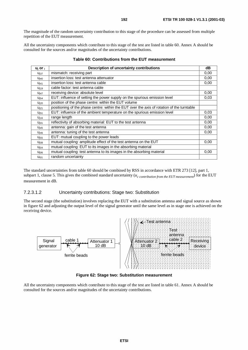
ETSI
ETSI TR 100 028-1 V1.3.1 (2001-03)192
The magnitude of the random uncertainty contribution to this stage of the procedure can be assessed from multiplerepetition of the EUT measurement.
All the uncertainty components which contribute to this stage of the test are listed in table 60. Annex A should beconsulted for the sources and/or magnitudes of the uncertainty contributions.
Table 60: Contributions from the EUT measurement
uj or i Description of uncertainty contributions dBuj37 mismatch: receiving part 0,00uj40 insertion loss: test antenna attenuator 0,00uj41 insertion loss: test antenna cable 0,00uj19 cable factor: test antenna cableuj47 receiving device: absolute level 0,00uj54 EUT: influence of setting the power supply on the spurious emission level 0,03uj20 position of the phase centre: within the EUT volumeuj21 positioning of the phase centre: within the EUT over the axis of rotation of the turntableuj51 EUT: influence of the ambient temperature on the spurious emission level 0,03uj16 range length 0,00uj01 reflectivity of absorbing material: EUT to the test antenna 0,00uj45 antenna: gain of the test antenna 0,00uj46 antenna: tuning of the test antenna 0,00uj55 EUT: mutual coupling to the power leadsuj08 mutual coupling: amplitude effect of the test antenna on the EUT 0,00uj04 mutual coupling: EUT to its images in the absorbing materialuj06 mutual coupling: test antenna to its images in the absorbing material 0,00ui01 random uncertainty
The standard uncertainties from table 60 should be combined by RSS in accordance with ETR 273 [12], part 1,subpart 1, clause 5. This gives the combined standard uncertainty (uc contribution from the EUT measurement) for the EUT
measurement in dB.
7.2.3.1.2 Uncertainty contributions: Stage two: Substitution
The second stage (the substitution) involves replacing the EUT with a substitution antenna and signal source as shownin figure 62 and adjusting the output level of the signal generator until the same level as in stage one is achieved on thereceiving device.
cable 1
ferrite beads
Attenuator 110 dB
Signalgenerator
Testantennacable 2
Test antenna
ferrite beads
Receivingdevice
Attenuator 210 dB
Figure 62: Stage two: Substitution measurement
All the uncertainty components which contribute to this stage of the test are listed in table 61. Annex A should beconsulted for the sources and/or magnitudes of the uncertainty contributions.
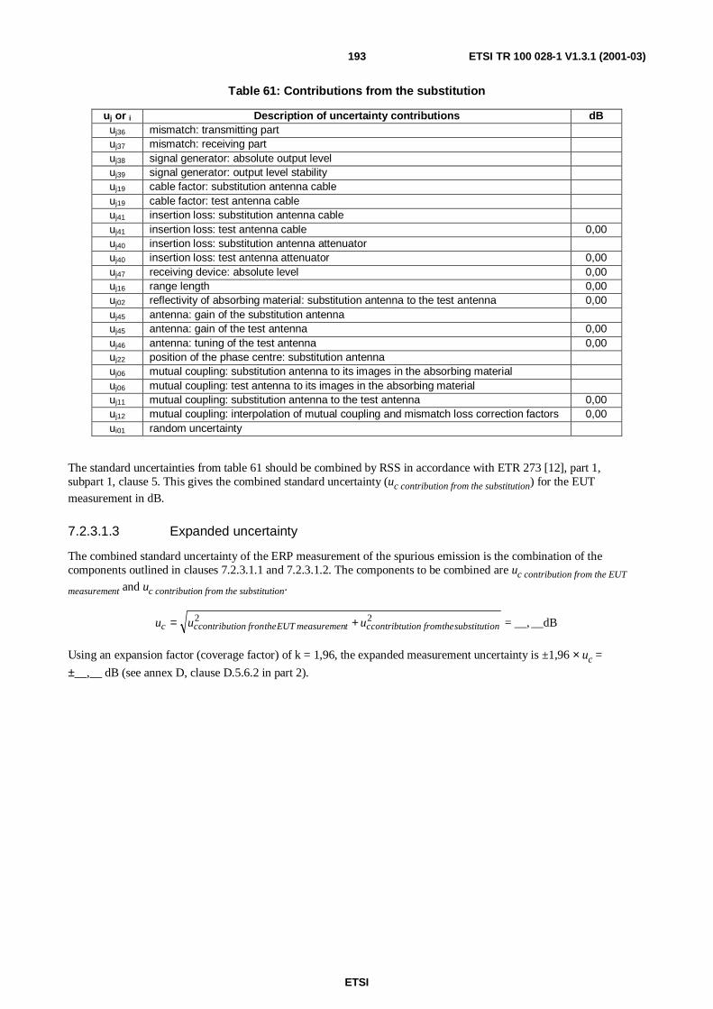
ETSI
ETSI TR 100 028-1 V1.3.1 (2001-03)193
Table 61: Contributions from the substitution
uj or i Description of uncertainty contributions dBuj36 mismatch: transmitting partuj37 mismatch: receiving partuj38 signal generator: absolute output leveluj39 signal generator: output level stabilityuj19 cable factor: substitution antenna cableuj19 cable factor: test antenna cableuj41 insertion loss: substitution antenna cableuj41 insertion loss: test antenna cable 0,00uj40 insertion loss: substitution antenna attenuatoruj40 insertion loss: test antenna attenuator 0,00uj47 receiving device: absolute level 0,00uj16 range length 0,00uj02 reflectivity of absorbing material: substitution antenna to the test antenna 0,00uj45 antenna: gain of the substitution antennauj45 antenna: gain of the test antenna 0,00uj46 antenna: tuning of the test antenna 0,00uj22 position of the phase centre: substitution antennauj06 mutual coupling: substitution antenna to its images in the absorbing materialuj06 mutual coupling: test antenna to its images in the absorbing materialuj11 mutual coupling: substitution antenna to the test antenna 0,00uj12 mutual coupling: interpolation of mutual coupling and mismatch loss correction factors 0,00ui01 random uncertainty
The standard uncertainties from table 61 should be combined by RSS in accordance with ETR 273 [12], part 1,subpart 1, clause 5. This gives the combined standard uncertainty (uc contribution from the substitution) for the EUTmeasurement in dB.
7.2.3.1.3 Expanded uncertainty
The combined standard uncertainty of the ERP measurement of the spurious emission is the combination of thecomponents outlined in clauses 7.2.3.1.1 and 7.2.3.1.2. The components to be combined are uc contribution from the EUT
measurement and uc contribution from the substitution.
__dB__,=22onsubstitutithefromioncontribtutctmeasuremenEUTthefrononcontributicc uuu +=
Using an expansion factor (coverage factor) of k = 1,96, the expanded measurement uncertainty is ±1,96 × uc =
±__,__ dB (see annex D, clause D.5.6.2 in part 2).

ETSI
ETSI TR 100 028-1 V1.3.1 (2001-03)194
7.2.3.2 Anechoic Chamber with a ground plane
7.2.3.2.1 Uncertainty contributions: Stage one: EUT measurement
For the measurement of spurious effective radiated power two stages of test are involved. The first stage (the EUTmeasurement) is to measure on the receiving device, a level from the EUT as shown in figure 63 (shaded componentsare common to both stages of the test).
Testantennacable 2
Test antenna
ferrite beads
EUT Attenuator 210 dB
Receivingdevice
Ground plane
Figure 63: Stage one: EUT measurement
Due to the commonality of all of the components from the test antenna to the receiver in both stages of the test, themismatch uncertainty contributes identically to both stages and hence cancels. Similarly, the systematic uncertaintycontributions (e.g. test antenna cable loss, etc.) of the individual components also cancel.
The magnitude of the random uncertainty contribution to this stage of the procedure can be assessed from multiplerepetition of the EUT measurement.
All the uncertainty components which contribute to this stage of the test are listed in table 62. Annex A should beconsulted for the sources and/or magnitudes of the uncertainty contributions.
Table 62: Contributions from the measurement on the EUT
uj or i Description of uncertainty contributions dBuj37 mismatch: receiving partuj19 cable factor: test antenna cable 0,00uj41 insertion loss: test antenna cable 0,00uj40 insertion loss: test antenna attenuator 0,00uj47 receiving device: absolute level 0,00uj54 EUT: influence of setting the power supply on the spurious emission levelsuj20 position of the phase centre: within the EUT volumeuj21 positioning of the phase centre: within the EUT over the axis of rotation of the turntableuj51 EUT: influence of the ambient temperature on the spurious emission leveluj16 range lengthuj18 correction: measurement distanceuj01 reflectivity of absorbing material: EUT to the test antennauj45 antenna: gain of the test antenna 0,00uj46 antenna: tuning of the test antenna 0,00uj55 EUT: mutual coupling to the power leadsuj08 mutual coupling: amplitude effect of the test antenna on the EUTuj04 mutual coupling: EUT to its images in the absorbing materialuj13 mutual coupling: EUT to its image in the ground planeuj06 mutual coupling: test antenna to its images in the absorbing materialuj14 mutual coupling: test antenna to its image in the ground planeui01 random uncertainty
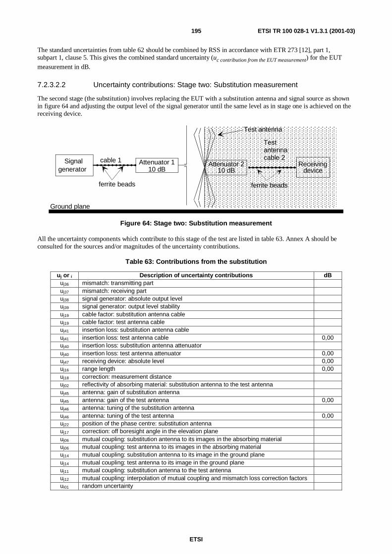
ETSI
ETSI TR 100 028-1 V1.3.1 (2001-03)195
The standard uncertainties from table 62 should be combined by RSS in accordance with ETR 273 [12], part 1,subpart 1, clause 5. This gives the combined standard uncertainty (uc contribution from the EUT measurement) for the EUT
measurement in dB.
7.2.3.2.2 Uncertainty contributions: Stage two: Substitution measurement
The second stage (the substitution) involves replacing the EUT with a substitution antenna and signal source as shownin figure 64 and adjusting the output level of the signal generator until the same level as in stage one is achieved on thereceiving device.
Testantennacable 2
Test antenna
ferrite beads
Attenuator 210 dB
Receivingdevice
cable 1
ferrite beads
Attenuator 110 dB
Signalgenerator
Ground plane
Figure 64: Stage two: Substitution measurement
All the uncertainty components which contribute to this stage of the test are listed in table 63. Annex A should beconsulted for the sources and/or magnitudes of the uncertainty contributions.
Table 63: Contributions from the substitution
uj or i Description of uncertainty contributions dBuj36 mismatch: transmitting partuj37 mismatch: receiving partuj38 signal generator: absolute output leveluj39 signal generator: output level stabilityuj19 cable factor: substitution antenna cableuj19 cable factor: test antenna cableuj41 insertion loss: substitution antenna cableuj41 insertion loss: test antenna cable 0,00uj40 insertion loss: substitution antenna attenuatoruj40 insertion loss: test antenna attenuator 0,00uj47 receiving device: absolute level 0,00uj16 range length 0,00uj18 correction: measurement distanceuj02 reflectivity of absorbing material: substitution antenna to the test antennauj45 antenna: gain of substitution antennauj45 antenna: gain of the test antenna 0,00uj46 antenna: tuning of the substitution antennauj46 antenna: tuning of the test antenna 0,00uj22 position of the phase centre: substitution antennauj17 correction: off boresight angle in the elevation planeuj06 mutual coupling: substitution antenna to its images in the absorbing materialuj06 mutual coupling: test antenna to its images in the absorbing materialuj14 mutual coupling: substitution antenna to its image in the ground planeuj14 mutual coupling: test antenna to its image in the ground planeuj11 mutual coupling: substitution antenna to the test antennauj12 mutual coupling: interpolation of mutual coupling and mismatch loss correction factorsui01 random uncertainty

ETSI
ETSI TR 100 028-1 V1.3.1 (2001-03)196
The standard uncertainties from table 63 should be combined by RSS in accordance with ETR 273 [12], part 1,subpart 1, clause 5. This gives the combined standard uncertainty (uc contribution from the substitution) for the EUT
measurement in dB.
7.2.3.2.3 Expanded uncertainty
The combined standard uncertainty of the ERP measurement of the spurious emission is the combination of thecomponents outlined in clauses 7.2.3.2.1 and 7.2.3.2.2. The components to be combined are uc contribution from the EUT
measurement and uc contribution from the substitution.
__dB__,=22onsubstitutithefromioncontribtutctmeasuremenEUTthefrononcontributicc uuu +=
Using an expansion factor (coverage factor) of k = 1,96, the expanded measurement uncertainty is ±1,96 × uc =
±__,__ dB (see annex D, clause D.5.6.2 in part 2).
7.2.3.3 Open Area Test Site
7.2.3.3.1 Uncertainty contributions: Stage one: EUT measurement
For the measurement of spurious effective radiated power two stages of test are involved. The first stage (the EUTmeasurement) is to measure on the receiving device, a level from the EUT as shown in figure 65 (shaded componentsare common to both stages of the test).
Testantennacable 2
Test antenna
ferrite beads
Attenuator 210 dB
Receivingdevice
EUT
Ground plane
Figure 65: Stage one: EUT measurement
Due to the commonality of all of the components from the test antenna to the receiver in both stages of the test, themismatch uncertainty contributes identically in each stage and hence cancels. Similarly, the systematic uncertaintycontributions (e.g. test antenna cable loss, etc.) of the individual components also cancel.
The magnitude of the random uncertainty contribution to each stage of the procedure can be assessed from multiplerepetition of the EUT measurement.
All the uncertainty components which contribute to this stage of the test are listed in table 64. Annex A should beconsulted for the sources and/or magnitudes of the uncertainty contributions.

ETSI
ETSI TR 100 028-1 V1.3.1 (2001-03)197
Table 64: Contributions from the measurement on the EUT
uj or i Description of uncertainty contributions dBuj37 mismatch: receiving partuj19 cable factor: test antenna cable 0,00uj41 insertion loss: test antenna cable 0,00uj40 insertion loss: test antenna attenuator 0,00uj47 receiving device: absolute level 0,00uj54 EUT: influence of setting the power supply on the spurious emission leveluj20 position of the phase centre: within the EUT volumeuj21 positioning of the phase centre: within the EUT over the axis of rotation of the turntableuj51 EUT: influence of the ambient temperature on the spurious emission leveluj16 range lengthuj18 correction: measurement distanceuj45 antenna: gain of the test antenna 0,00uj46 antenna: tuning of the test antenna 0,00uj55 EUT: mutual coupling to the power leadsuj08 mutual coupling: amplitude effect of the test antenna on the EUTuj13 mutual coupling: EUT to its images in the ground planeuj14 mutual coupling: test antenna to its images in the ground planeui01 random uncertainty
The standard uncertainties from table 64 should be combined by RSS in accordance with ETR 273 [13], part 1,subpart 1, clause 5. This gives the combined standard uncertainty (uc contribution from the EUT measurement) for the EUT
measurement in dB.
7.2.3.3.2 Uncertainty contributions: Stage two: Substitution measurement
The second stage (the substitution) involves replacing the EUT with a substitution antenna and signal source as shownin figure 66 and adjusting the output level of the signal generator until the same level as in stage one is achieved on thereceiving device.
Testantennacable 2
Test antenna
ferrite beads
Attenuator 210 dB
Receivingdevice
cable 1
ferrite beads
Attenuator 110 dB
Signalgenerator
Ground plane
Figure 66: Stage two: Typical emission substitution test
All the uncertainty components which contribute to this stage of the test are listed in table 65. Annex A should beconsulted for the sources and/or magnitudes of the uncertainty contribution.

ETSI
ETSI TR 100 028-1 V1.3.1 (2001-03)198
Table 65: Contributions from the substitution
uj or i Description of uncertainty contributions dBuj36 mismatch: transmitting partuj37 mismatch: receiving partuj38 signal generator: absolute output leveluj39 signal generator: output level stabilityuj19 cable factor: substitution antenna cableuj19 cable factor: test antenna cableuj41 insertion loss: substitution antenna cableuj41 insertion loss: test antenna cable 0,00uj40 insertion loss: substitution antenna attenuatoruj40 insertion loss: test antenna attenuator 0,00uj47 receiving device: absolute level 0,00uj16 range length 0,00uj18 correction: measurement distanceuj45 antenna: gain of the substitution antennauj45 antenna: gain of the test antenna 0,00uj46 antenna: tuning of the substitution antennauj46 antenna: tuning of the test antenna 0,00uj22 position of the phase centre: substitution antennauj17 correction: off boresight angle in the elevation planeuj14 mutual coupling: substitution antenna to its image in the ground planeuj14 mutual coupling: test antenna to its image in the ground planeuj11 mutual coupling: substitution antenna to the test antennauj12 mutual coupling: interpolation of mutual coupling and mismatch loss correction factorsui01 random uncertainty
The standard uncertainties from table 65 should be combined by RSS in accordance with ETR 273 [12], part 1,subpart 1, clause 5. This gives the combined standard uncertainty (uc contribution from the substitution) for the EUT
measurement in dB.
7.2.3.3.3 Expanded uncertainty
The combined standard uncertainty of the ERP measurement of the spurious emission is the combination of thecomponents outlined in clauses 7.2.6.1 and 7.2.6.2. The components to be combined are uc contribution from the EUT
measurement and uc contribution from the substitution.
__dB__,=22onsubstitutithefromioncontribtutcmesurementEUTthefrononcontributicc uuu +=
Using an expansion factor (coverage factor) of k = 1,96, the expanded measurement uncertainty is ±1,96 × uc =
±__,__ dB (see annex D, clause D.5.6.2 in part 2).
7.2.3.4 Stripline
This test is not usually performed in a Stripline and is therefore not considered here.
7.2.3.5 Test fixture
This test is not normally carried out in a test fixture.
7.2.4 Adjacent channel power
7.2.4.1 Anechoic Chamber
This test is normally carried out using a test fixture and as a result has not been considered for the Anechoic Chamber.

ETSI
ETSI TR 100 028-1 V1.3.1 (2001-03)199
7.2.4.2 Anechoic Chamber with a ground plane
This test is normally carried out using a test fixture and as a result has not been considered for the Anechoic Chamberwith a ground plane.
7.2.4.3 Open Area Test Site
This test is normally carried out using a test fixture and as a result has not been considered for the Open Area Test Site.
7.2.4.4 Stripline
This test is normally carried out using a test fixture and as a result has not been considered for the Strip line.
7.2.4.5 Test fixture
The uncertainty contributions for the test are shown in table 66.
NOTE: Some standards require the adjacent channel power to be 60 dBc without the need for it to fall below250 nW. In this case, both values (absolute and dBc) are required as, for example, 40 dBc is consideredsatisfactory if the adjacent channel power is < 250 nW.
7.2.4.5.1 Contributions from the measurement
Table 66: Contributions from the measurement
uj or i Description of uncertainty contributions dBuj48 receiving device: linearityuj49 receiving device: power measuring receiveruj50 EUT: influence of the ambient temperature on the ERP of the carrieruj53 EUT: influence of setting the power supply on the ERP of the carrieruj60 Test Fixture: effect on the EUTuj61 Test Fixture: climatic facility effect on the EUTui01 random uncertainty
The standard uncertainties from table 66 should be given values according to annex A. They should then be combinedby RSS in accordance with ETR 273 [12], part 1, subpart 1, clause 5. This gives the combined standard uncertainty(uc contributions from the measurement) for the EUT measurement in dB.
7.2.4.5.2 Expanded uncertainty
For a relative measurement (dBc) of adjacent channel power, the combined uncertainty, uc, of the measurement issimply the value for uc contributions from the measurement derived above.
Using an expansion factor (coverage factor) of k = 1,96, the expanded measurement uncertainty is ±1,96 × uc =
±__,__ dB (see annex D, clause D.5.6.2 in part 2).
For those test standards that require the adjacent channel power to be given in absolute terms, however, for thecalculation of the measurement uncertainty, the Test Fixture measurement should be considered as stage two of a test inwhich stage one was on an accredited Free-Field Test Site. The combined standard uncertainty, uc, of the adjacentchannel power measurement is therefore, simply the RSS combination of the value for uc contributions from the measurement
derived above and the combined uncertainty of the Free-field Test Site uc contribution from the Free-Field Test Site.
dB____,22 =+= − sitetestfieldfreethefromonscontributictmeasurementhefromonscontributicc uuu
Using an expansion factor (coverage factor) of k = 1,96, the expanded measurement uncertainty is ±1,96 × uc =
±__,__ dB (see annex D, clause D.5.6.2 in part 2).

ETSI
ETSI TR 100 028-1 V1.3.1 (2001-03)200
History
Document history
Edition 1 March 1992 Publication as ETR 028
Edition 2 March 1994 Publication as ETR 028
V1.3.1 March 2001 Publication