Towards better computation-statistics trade-off in tensor decomposition

Ryota Tomioka TTI Chicago

Joint work with: T. Suzuki, K. Hayashi, & H. Kashima

Matrices and Tensors in machine learning

Sens

ors

Time Multivariate time-series Collaborative filtering

Star  Wars

Titanic Blade  Runner

User  1   5 2 4

User  2 1 4 2

User  3 5 ? ?

Movies

User

s

Spatio-temoral data Multiple relations

Watch

Buy

Like

Mat

rices

Tens

ors

Matrices and Tensors in machine learning

Sens

ors Time

Multivariate time-series Collaborative filtering

Movies

User

s

Spatio-temoral data Multiple relations

Mat

rices

Tens

ors

Sens

ors

User

s

From matrices to tensors •  Trace norm: convex relaxation of matrix rank

–  It works like L1 regularization on the singular values

–  Performance guarantees [Srebro & Schraibman 2005; Candes & Recht 2009; Candes & Tao 2010; Negahban & Wainwright 2011]

Induces low-rank-ness (spectral sparsity)

�W �S1 =r�

j=1

�j(W )

Similar  relaxa2on  possible  for  tensor  rank?  

From matrices to tensors

•  Spectral norm of random Gaussian matrix

•  Marchenko-Pastur� distribution�[Marchenko & Pastur 1967]

EkXkS1 ��p

m+pn�

0 50 100 150 2000

5

10

15

20

25

30

35

40

Order

Sin

gu

lar

va

lue

s

Gaussian, size=[200 500]

0 50 100 150 2000

5

10

15

20

25

30

35

40

Order

Sin

gu

lar

va

lue

s

Uniform, size=[200 500]

empirical spectrum

theory

empirical spectrum

theory

Random  tensor  theory?  

Outline

•  Tensor ranks and decompositions

•  Overlapped trace norm (moderate computation) –  Limitations: requires O(rnK-1) samples

•  Balanced trace norm (heavy computation) [Mu et al. 2013] –  requires O(rK/2nK/2) samples

•  Tensor trace norm (probably intractable) –  requires only O(rn) samples

Tensor rank •  Minimum number R such that

•  Known as CP (canonical polyadic) decomposition [Hitchcock  27; Carroll & Chang 70; Harshman 70]

•  Comutation of the above decomposition is NP hard!

n1

n2 n3

= R�

r=1ar

br

cr

�Xijk =

R�

r=1

airbjrckr

�

(for  3rd  order  tensor)  

Tucker decomposition

n1

n2 n3

�Xijk =

r1⇤

a=1

r2⇤

b=1

r3⇤

c=1

CabcU(1)ia U (2)

jb U (3)kc

⇥r1 r2

r3 = �1 �2 �3

n1 r1

n2 r2

n3 r3

Core Factors

•  Factors can be obtained by unfolding operation+SVD •  In practice no unfolding is low-rank --- Common solution: iterate

truncated SVD (HOSVD, HOOI); non-convex

[Tucker 66; De Lathauwer+00]

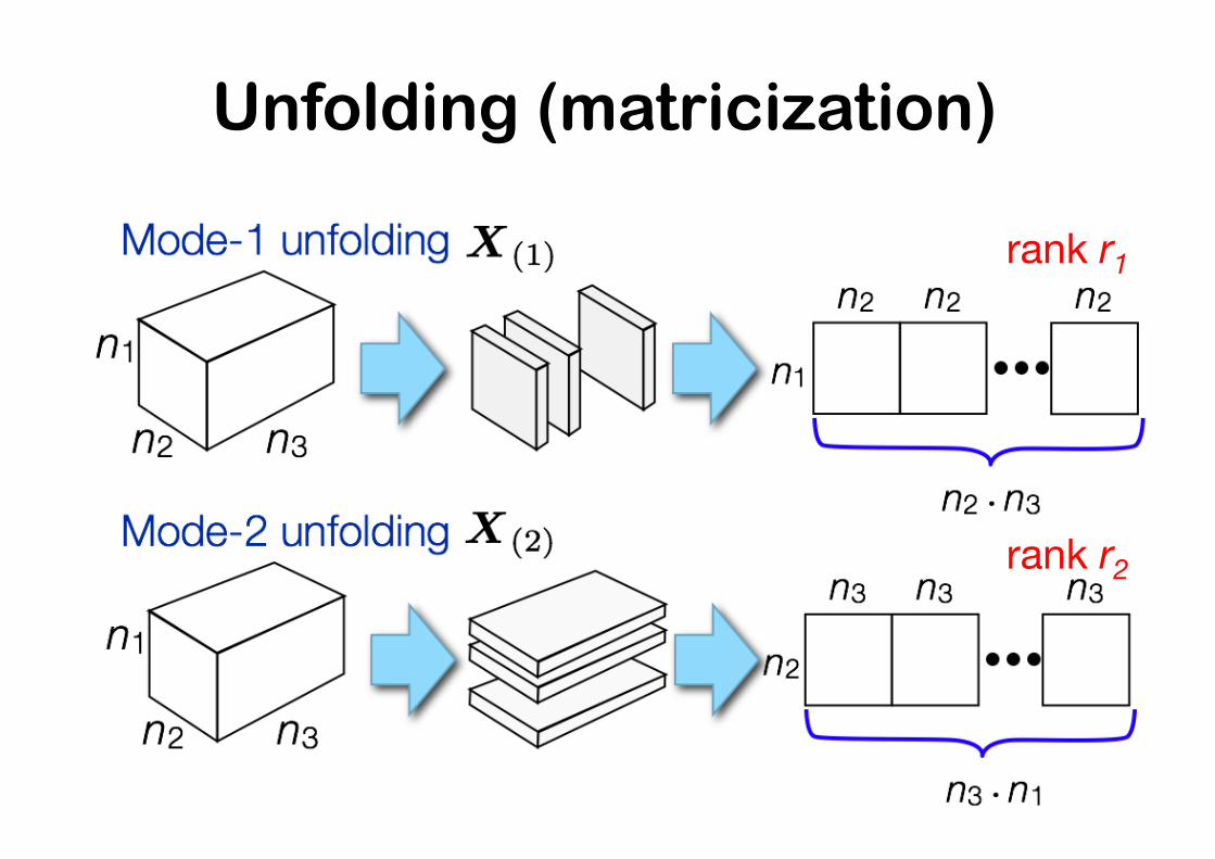
Unfolding (matricization)

rank r1

rank r2

Core idea

Tensor  X  is  low  rank  ∃k,  rk  <  nk  

(in  the  sense  of  Tucker  decomposi2on)

Unfolding  X(k)  is  low-­‐rank  (as  a  matrix)

Unfolding (Matricization)

Tensorization

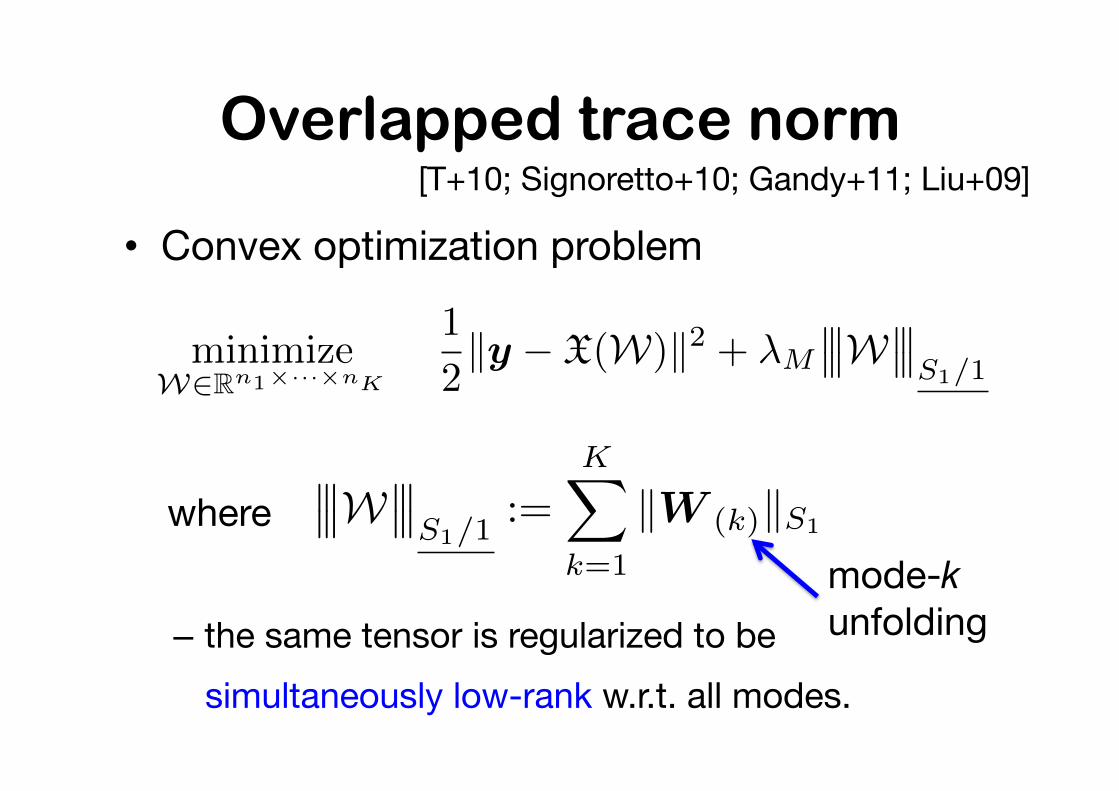
Overlapped trace norm

•  Convex optimization problem

–  the same tensor is regularized to be simultaneously low-rank w.r.t. all modes.

minimizeW2Rn1⇥···⇥nK

1

2ky � X(W)k2 + �M

������W������S1/1

������W������S1/1

:=KX

k=1

kW (k)kS1where

mode-k unfolding

[T+10; Signoretto+10; Gandy+11; Liu+09]

0 0.1 0.2 0.3 0.4 0.5 0.6 0.7 0.8 0.9 1

10−4

10−3

10−2

10−1

100

Fraction of observed elements

Gen

eral

izat

ion

erro

r

As a Matrix (mode 1)As a Matrix (mode 2)As a Matrix (mode 3)OverlapLatentTucker (large)Tucker (exact)Optimization tolerance

Empirical performance •  True tensor: 50x50x20, rank 7x8x9. No noise (λ=0).

•  Random train/test split.

Tucker = EM algo (non-convex) [Andersson & Bro 00]

Phase transition!

Analysis: Problem setting Observation

Gaussian noise N(0,σ2) Optimization

Reg. constant

Observation operator X(W) = (�X 1, W� , . . . , �X M , W�)�

Likelihood Regularization

(N =�K

k=1 nk)X : RN � RM

: true tensor with rank (r1,...,rK) W⇤

yi = hXi,W⇤i+ ✏i (i = 1, . . . ,M)

W = argminW2Rn1⇥···⇥nK

✓1

2ky � X(W)k2 + �M

������W������S1/1

◆

Theorem (“overlapped” approach) 　Assume  that  the  elements  of  the  design  X  are  independently  and  iden2cally  Gaussian  distributed.  

Moreover,  if  

#samples (M)

#variables (N)� c1⇥n�1⇥1/2⇥r⇥1/2 �

r

nnormalized rank

�n�1�1/2 :=�

1K

�Kk=1

�1/nk

�2, �r�1/2 :=

�1K

�Kk=1

�rk

�2

[T, Suzuki, Hayashi, Kashima 11]

Theorem (random Gauss design) 　Assume  that  the  elements  of  the  design  X  are  independently  and  iden2cally  Gaussian  distributed.  

Moreover,  if  

#samples (M)

#variables (N)� c1⇥n�1⇥1/2⇥r⇥1/2 �

r

nnormalized rank

�n�1�1/2 :=�

1K

�Kk=1

�1/nk

�2, �r�1/2 :=

�1K

�Kk=1

�rk

�2

������W �W�������2F

N� Op

��2�n�1�1/2�r�1/2

M

�Convergence!

[T, Suzuki, Hayashi, Kashima 11]

(with appropriate choice of λM)

Tensor completion

0 0.2 0.4 0.6 0.8 1

10−3

100

Fraction of observed elements

Estim

atio

n e

rro

r

Convex [7 8 9]

Covex [40 9 7]

Optimization tolerance

0 0.2 0.4 0.6 0.80

0.2

0.4

0.6

0.8

1

Normalized rank ||n−1||1/2||r||1/2

Frac

tion

at E

rror<

=0.0

1

size=[50 50 20]size=[100 100 50]

No observation noise Normalized rank

Fraction M/N at

error<=0.01

rank=[7,8,9] 0.01

size = 50x50x20 true rank 7x8x9 or 40x9x7

rank=[40,9,7] #samples (M)

#variables (N)

Theory vs. Experiments (4th order)

0 0.2 0.4 0.6 0.8 10

0.2

0.4

0.6

0.8

1

Normalized rank ||n−1||1/2||r||1/2

Frac

tion

at e

rr<=0

.01

size=[50 50 20]size=[100 100 50]size=[50 50 20 10]size=[100 100 20 10]

Limitation: exponentially many samples required!

•  Simplify by setting nk=n and rk=r

•  Then there are constants c0, c1, c2 such that – #samples

–  reg. const. �M = c0�q

nK�1/M

������W �W⇤������2F c2

�2rnK�1

M

with high probability.

M � c1nK�1r

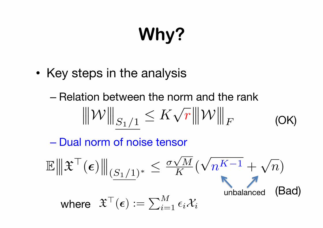
Why?

•  Key steps in the analysis

– Relation between the norm and the rank

– Dual norm of noise tensor

(OK) ������W

������S1/1

Kpr������W

������F

where X>(✏) :=PM

i=1 ✏iXi

(Bad) unbalanced

E������X>(✏)

������(S1/1)⇤

�pM

K (pnK�1 +

pn)

Balanced unfolding

•  For K>3, there are 2K-1-1 > K ways to unfold a tensor. For example,

n1

n1

n3 n3

n1n2

n3n4

X(1,2;3,4) =

(See also Mu et al. 2013)

Balanced trace norm (for K=4) •  Definition

– Relation between the norm and the rank

– Dual norm of noise tensor E������X>(✏)

������balanced⇤ �

pM

3 · 2pn2

������W������balanced

3pr2������W

������F

Sample complexity O(r2n2)

������W������balanced

:= kW (1,2;3,4)kS1 + kW (1,3;2,4)kS1 + kW (1,4;2,3)kS1

5 10 20 30

103

104

105

Mc=4.5 n2.93

Mc=23.3 n2.08

Dimension n

Num

ber o

f sam

ples

at t

he p

hase

tran

sitio

n

Overlapped (balanced)Overlapped (unbalanced)

Experiment (K=4) Theoretically × O(n3) △ O(n2)

tensor completion at rank (2,2,2,2)

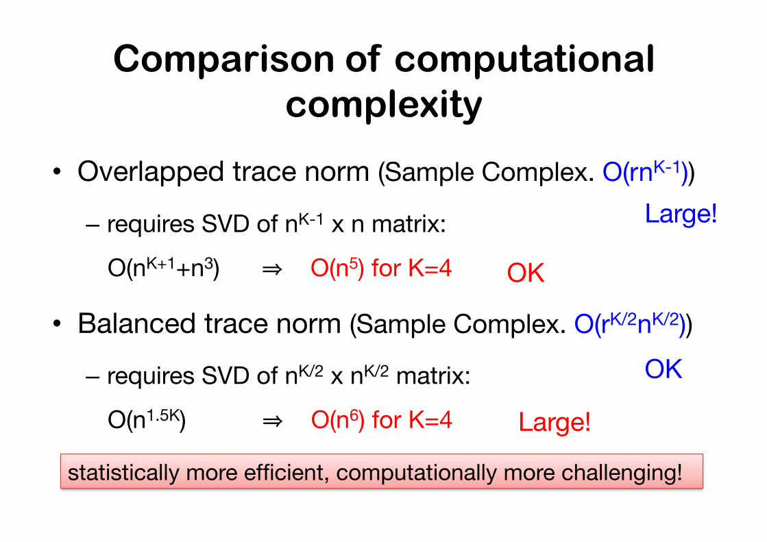
Comparison of computational complexity

•  Overlapped trace norm (Sample Complex. O(rnK-1)) –  requires SVD of nK-1 x n matrix:�

O(nK+1+n3) ⇒ O(n5) for K=4

•  Balanced trace norm (Sample Complex. O(rK/2nK/2)) –  requires SVD of nK/2 x nK/2 matrix:�

O(n1.5K) ⇒ O(n6) for K=4

statistically more efficient, computationally more challenging!

Large!

OK

OK

Large!

Computation-statistics trade-off Sample complexity

Computational complexity

nK

nK-1

nK/2

nK nK+1 n3K/2

Frobenius norm

Overlapped trace norm

Balanced trace norm

?

W

Tensor trace norm For K=3

rank-1 tensor (outer prod. of vectors)

can  be  seen  as  an  atomic  norm  [Chandrasekaran  12]  with    atomic  set  =  set  of  rank-­‐1  tensors

������W������tr 1

������W������tr= inf

X

a2Aca s.t. W =

X

a2Acaua � va �wa

ca � 0

kuk 1, kvk 1, kwk 1

Tensor trace norm For K=3 ������W������tr= inf

X

a2Aca s.t. W =

X

a2Acaua � va �wa

ca � 0

Relation between the norm and the orthogonal CP rank (Kolda 2001) ������W

������tr

pR������W

������F

kuk 1, kvk 1, kwk 1

Dual norm of the noise tensor

Sample complexity O(Rn)

E������X>(✏)

������tr⇤

C�pM

pn

Dual of the trace norm is the tensor operator norm

s.t. kuk 1, kvk 1, kwk 1

������Y������tr

⇤ =������Y

������op

:= supu,v,w

X

i,j,k

Yijkuivjwk

Greedy algorithm for computing the operator norm 1.  Initialize u, v, w. 2.  Fix u, maximize over v and w (matrix operator norm) 3.  Cycle over v, w, u, … until convergence (can be improved by incorporating gradient)

10,000 random restarts

15.4 15.6 15.8 16 16.2 16.4 16.6 16.8 17 17.20

200

400

600

800

1000

1200

1400

Operator norm

Freq

uenc

yOperator norm of a random 50x50x20 tensor

Empirical scaling (K=3)

101 102 103100

101

102

103

2.54x0.52

1.02x1.00

Dimensionality n1=n2=n3

Norm

s

Operator normDual overlap norm

Theoretically × O(n) ｘ O(√n)

Low-rank tensor estimation with the tensor trace norm

minimizeW2Rn1⇥···⇥nK

1

2ky � X(W)k2 + �M

������W������tr

Likelihood Regularization

Key operation: prox operator

= W � proj�(W) (Moreau’s theorem)

Tensor operator norm

proj�(W) = argmin

Y

������W � Y������F

s.t.������Y

������op

�

prox�(W) = argmin

Y

✓�������Y

������tr+

1

2

������Y �W������2F

◆

Greedy algorithm for proxλ(W)

1.  Let R=W.

2.  Compute ||R||op�if ||R||op ≤ λ, done. Return W-R�otherwise, R=R+(λ-||R||op) u・v・w

3.  Go to 2.�

Tensor completion experiment

0 0.2 0.4 0.6 0.8 1−0.2

0

0.2

0.4

0.6

0.8

Fraction of observed elements

Gen

eral

izat

ion

erro

r

As a matrixOverlapAtomicPARAFAC (large)PARAFAC (exact)

size=50x50x20, CP rank=8 (mode 1)

(λ→0)

PARAFAC implemented in N-way toolbox [Andersson & Bro 00]

tensor trace norm

Balanced vs. unbalanced

0 0.2 0.4 0.6 0.8 1−0.2

0

0.2

0.4

0.6

0.8

Fraction of observed elements

Gen

eral

izat

ion

erro

r

As a matrixOverlapAtomicPARAFAC (large)PARAFAC (exact)L2Ball

size=25x5x5, CP rank=3

balanced 25x25

(mode 1)

(λ→0)

PARAFAC implemented in N-way toolbox [Andersson & Bro 00]

Summary •  Tensor decomposition via convex optimization

–  Fast and stable algorithm for tensor decomposition –  Rank selection is replaced by regularization parameter selection

•  Limitation of the overlapped trace norm –  unbalancedness of the unfolding –  balanced unfolding

•  Optimization statistics trade-off –  balanced trace norm requires less samples but more computation –  tensor trace norm requires only O(n) samples but seems intractable

References •  Andersson and Bro. (2000) The n-way toolbox for matlab. Chemometrics & Intelligent Laboratory Systems, 52(1):1–4, 2000. http://

www.models.life.ku.dk/source/nwaytoolbox/.

•  Chandrasekaran, Recht, Parrilo, and Willsky. (2012) The convex geometry of linear inverse problems. Foundations of Computational Mathematics, 12(6):805–849.

•  Kolda & Bader (2009) Tensor Decompositions and Applications. SIAM Review.

•  Gandy, Recht, and Yamada. (2011) Tensor completion and low-n-rank tensor recovery via convex optimization. Inverse Problems,

27:025010.

•  Håstad. (1990) Tensor rank is NP-complete. Journal of Algorithms, 11(4):644– 654.

•  Mu, Huang, Wright, and Goldfarb. (2013) Square deal: Lower bounds and improved relaxations for tensor recovery. arXiv preprint arXiv:1307.5870.

•  Signoretto, De Lathauwer, and Suykens. (2010) Nuclear norms for tensors and their use for convex multilinear estimation. Technical Report

10-186, ESAT-SISTA, K.U.Leuven.

•  Tomioka, Suzuki, Hayashi, and Kashima. (2011) Statistical performance of convex tensor decomposition. In Advances in NIPS 24, pages

972–980.

•  Tomioka and Suzuki. (2013) Convex tensor decomposition via structured schatten norm regularization. In Advances in NIPS 26, pages 1331–1339.

•  Tomioka, Suzuki, Hayashi, & Kashima. (2014) Low-Rank Tensor Denoising and Recovery via Convex Optimization. In Suykens, Signoretto, & Argyriou, editors, Regularization, Optimization, Kernels, and Support Vector Machines. To be published from CRC Press.

T h n a k y u o !