Towards Automatic Software Lineage Inference

Abstract—Software continuously evolves to reflect changingrequirements, feature updates, and bug fixes. Most existingresearch focuses on analyzing software release histories tounderstand the software evolution process and to describeevolutionary relationships among programs. However, therehas been little research on inferring software lineage from(binary) programs.

In this paper, we take a systematic approach towards soft-ware lineage inference. We explore three fundamental questionsnot addressed by existing work. First, how do we measure thequality of a lineage inference algorithm? Second, given existingapproaches to binary similarity analysis, how good are they forlineage both currently and in an idealized setting? Third, whatare the challenging problems in software lineage inference?Towards these goals we build LIMetric—a system for automaticsoftware lineage inference of binary programs. We evaluatedLIMetric on two types of lineage—straight line lineage anddirected acyclic graph (DAG) lineage. We have also extendedour technique to handle multiple straight line lineages. Ourexperiments used large scale real-world programs, with a totalof 1,777 releases spanning over a combined 110 years ofdevelopment history. In order to quantify lineage quality, wepropose four metrics: (i) number of inversions and (ii) editdistance to monotonicity for straight line lineage, and (iii)number of lowest common ancestor (LCA) mismatches and(iv) average pairwise distance to true LCA for DAG lineage.LIMetric effectively extracted software derivation relationshipsamong binary programs with high accuracy. Through closecase analysis, we also formulate several challenging problemsin software lineage inference that need to be addressed to attaineven higher accuracy.

Keywords-software evolution, software lineage, systematicevaluation

I. INTRODUCTION

Software evolves to adapt to changing needs, bug fixes,and feature requests [18]. The lineage of software through itsevolution provides a potentially rich source of informationfor a number of security questions. For example, given acollection of malware variants, which malware came first?Given a collection of binaries in forensics, are any ofthem derived from the others? These kinds of questions areimportant enough that the US Defense Advanced ResearchProjects Agency (DARPA) is spending $43 million to studythem [1]. Unfortunately, existing work has primarily focusedon analyzing known lineage, not inferring lineage. For exam-ple, Belady and Lehman studied software evolution of IBMOS/360 [5], and Lehman and Ramil formulated eight lawsdescribing software evolution process [18]: 1) continuingchange, 2) increasing complexity, 3) self regulation, 4)conservation of organisational stability, 5) conservation offamiliarity, 6) continuing growth, 7) declining quality, and8) feedback system. With a wealth of release informationsuch as release dates and program versions, researchers haveanalyzed histories of open source projects [28], Firefox [21],

and Linux kernel [10] in order to verify Lehman’s laws ofsoftware evolutions and to understand software evolutionprocess.

The security community has studied malicious software(malware) evolution based upon the observation that themajority of incoming malware are tweaked variants of well-known malware [4, 12, 13]. With over 1.1 million malwareappearing in one day [2], researchers have studied such evo-lutionary relationships to identify new variants of previously-analyzed malware [8], to understand the diversity of exploitsused by notorious worms [20], and to generate phylogenymodels to describe derivation relationships among programsas a dendrogram [14, 15].

The task of software lineage inference is to infer a tem-poral ordering and ancestor/descendant relationships amongprograms. Software lineage can be defined as follows:

Definition I.1. A lineage graph G = (N,A) is a directedacyclic graph (DAG) comprising a set of nodes N and a setof arcs A. A node n ∈ N represents a program, and an arca = (x, y) ∈ A denotes that program y is a derivative ofprogram x. We say that x is a predecessor of y and y is asuccessor of x.

We define some terminology. A root is a node that has noincoming arc and a leaf is a node that has no outgoing arc.Since a DAG can have multiple roots, we introduce a newnode called the super root and add a new arc from it to everyroot. A DAG that has been augmented in this way is called asuper DAG. Note that a root in a super DAG has exactly oneincoming arc from the super root. An ancestor of a node n isa node that can reach n. Note that n is an ancestor of itself.A common ancestor of x and y is the intersection of thetwo sets of ancestors. In a DAG, a lowest common ancestor(LCA) of two nodes x and y is a common ancestor of xand y that is not an ancestor to another common ancestorof x and y [6]. Notice that there can be multiple LCAs. Wedenote the set of LCAs of x and y as SLCA(x, y).

In this paper, we ask three basic research questions:• What are good metrics? Existing research focused on

building phylogeny of malware [14, 15], but has lackedquality metrics to scientifically measure the quality oftheir output.Good metrics are necessary to assess how good ourapproach is with respect to the ground truth. Goodmetrics also allow us to quantify the quality of ouroutput, and to compare different approaches.

• How well are we doing now? We would like tounderstand what are the limits of existing techniqueseven in ideal cases, meaning we have 1) control overvariables affecting the compilation of programs such

Software Lineage Inference

Features 9

Straight Line Lineage DAG Lineage

Section Size

File Size

Cyclomatic Complexity

n-grams

Disassembly Instructions

Mnemonics with operands types

Normalized Mnemonics

Sorted Normalized Mnemonics

Hybrid

Root Revision 2

Inferred Root

Real Root

Timestamp 3

No Timestamp

Pseudo Timestamp

Real Timestamp

Features 1

Hybrid

Root Revision 2

Inferred Root

Real Root

Quality Metrics 2

Number of Inversions

Edit Distance to Monotonicity

Quality Metrics 2

Number of LCA Mismatches

Average Distance to True LCA

Datasets 3

Contiguous Revisions

Released Versions

Released Binaries

Datasets 1

DAG-like Revisions

Figure 1: Design space in software lineage inference

as compiler versions and optimization options so thatbinary code compiled from similar source code wouldbe similar, 2) reliable feature extraction techniquesto abstract binary programs accurately and precisely,which is not always guaranteed due to the difficulty ofdisassembling, and 3) the ground truth with which wecan compare our results to measure accuracy and tospot error cases.Although previous approaches have focused on mal-ware, we argue that it is necessary to first system-atically validate a lineage inference technique with“goodware”, e.g., open source projects. Since malwareis often surreptitiously developed by adversaries, it ishard or even impossible to obtain the ground truth.Furthermore, we cannot hope to understand evolutionon adversarial programs unless we first understandlimits of our approach without an adversary. To the bestof our knowledge, no systematic experiment addressingall the variables has been done before.

• What are the challenging problems? We need toidentify challenging problems in order to improve soft-ware lineage inference techniques. We should evaluatewith an eye towards uncovering fundamental limits orproblems. Previous work has not addressed this.

In this paper, we propose techniques and metrics for thesystematic investigation on software lineage as describedin Figure 1. We explore two types of lineage: straightline lineage and directed acyclic graph (DAG) lineage. In

addition, we extend our approach for straight line lineage tok-straight line lineage.• Four metrics to measure quality. We propose two

metrics for straight line lineage: number of inversionsand edit distance to monotonicity. Given an inferredgraph G and the ground truth G∗, the number ofinversions measures how often we get the question“which one of program pi and program pj comes first”wrong. The edit distance to monotonicity asks “howmany nodes do we need to remove in G such that theremaining nodes are in sorted order and thus respectG∗”.We also propose two metrics for DAG lineage: numberof LCA mismatches and average pairwise distance totrue LCA. An LCA mismatch is a generalized version ofan inversion because the LCA of two nodes in a straightline is the earlier node. In case we have a wrong LCA,we also measure the average pairwise distance betweenthe true LCA(s) and the derived LCA(s) in G∗. Thisdetailed measurement is desirable because it often helpsus to decide which of methods is better even when theirLCA scores are the same.

• Large scale systematic evaluation. We systematicallyevaluated LIMetric with goodware that we have groundtruth. For straight line lineage, we collected three kindsof datasets: 1) contiguous revisions from a versioncontrol system with highly varying time gap betweenadjacent commits (<10 minutes to over a month)—

371 revisions from 3 programs representing 4 yearsof combined history, 2) released versions distributed toend users, meaning that experimental features that con-tiguous revisions may have are excluded—271 releasesfrom 5 programs representing 55 years of combinedhistory, and 3) actual released binary programs fromdeb or rpm package files where we do not haveany control over the compiling process—355 releasesfrom 7 programs representing 40 years of combinedhistory. Regarding DAG lineage experiments, we down-loaded revision histories that have multiple branchingand merging points—780 revisions from 10 programsrepresenting 11 years of combined history.We also examined the effectiveness of different exper-iment policies: 1) whether we infer the root/earliestrevision or use the given real root revision, and 2)whether we rely on pseudo timestamp, real timestamp,or nothing. The second policy is only for DAG lineage.

• Challenging problems. We investigate error cases inG constructed by LIMetric and highlight some of thedifficult cases where LIMetric failed to recover thecorrect evolutionary relationships. We also discuss whatchallenging problems need to be addressed to achievehigher accuracy in software lineage inference.

II. OVERVIEW

Our goal is to systematically explore the entire designspace illustrated in Figure 1 to understand the advantagesand disadvantages of existing techniques for inferring soft-ware lineage. We have built LIMetric for systematic inves-tigation on software lineage in three different scenarios: 1-straight line lineage (§II-C), k-straight line lineage (§II-D),and directed acyclic graph (DAG) lineage (§II-E).

A. Software Features for Software Lineage

We evaluate the accuracy of software lineage inferenceon diverse input datasets that have different characteristics:contiguous revisions, released versions, released binaries,and DAG-like revisions. Given a set of binary programs P ,various features fi are extracted from each program pi ∈ Pto evaluate different abstractions of binary programs. Sourcecode or metadata such as comments, commit messages ordebugging information is not used as we are interested inresults in security scenarios where source code is typicallynot available, e.g., computer forensics, proprietary software,and malware.

We would like to evaluate existing approaches for ab-stracting binary programs in idealized settings, meaningthat we have reliable feature extraction techniques. Thereare mainly three program analysis methods: syntax-basedanalysis, static analysis, and dynamic analysis. In this study,we leave dynamic analysis-based features out of our scopeand include techniques using only syntax-based analysis andstatic analysis. The limitation with static analysis comes

from the difficulty of getting precise disassembly outputsfrom binary programs [17, 19]. In order to exclude theerrors introduced at the feature extraction step and focus onevaluating the performance of a software lineage inferencealgorithm, we also leverage assembly obtained using gcc-S (not source code itself) to obtain basic blocks moreaccurately. Note we use this to simulate what the resultswould be with an ideal disassembler, in line with our goalof understanding the limits of the selected approaches.

1) Using Previous Observations on Software Evolution:Previous work analyzed software release history to under-stand the software evolution process. It has been oftenobserved that program size and complexity tend to increaseas new revisions are released [10, 18, 28]. This observationalso carries over to security scenarios, e.g., the complexityof malware is likely to grow as new variants appear [7].

We measured code section size, file size, and code com-plexity to assess how useful these features are in inferringlineage of binary programs.• Section size: LIMetric first identifies executable sec-

tions in binary code, typically the .text sections,which contain executable program code, and calculatesthe total size.

• File size: Besides the section size, LIMetric also cal-culates the file size, including code and data.

• Cyclomatic complexity: Cyclomatic complexity [22]is a common metric that indicates code complexity bymeasuring the number of linearly independent paths.From the control flow graph (CFG) of a program, thecomplexity M is defined as:

M = E −N + 2P

where E is the number of edges, N is the number ofnodes, and P is the number of connected componentsof the CFG.

2) Using Syntax-based Feature: Although syntax-basedanalysis may lack semantic understanding of a program,previous work has shown its effectiveness on classifyingunpacked binary code. Indeed, n-gram analysis is widelyadopted to software similarity detection, e.g., [13, 14, 16,25]. The benefit of syntax-based analysis is that it is fast.This is because it does not require disassembling binarycode.• n-grams: An n-gram is a consecutive subsequence of

n items in a sequence. From the identified executablesections, LIMetric extracts program code in a hexadec-imal format, then n-grams are obtained by sliding awindow of n-bytes over the extracted byte sequence ofprogram code. For example, Figure 2(b) shows 4-gramsextracted from Figure 2(a).

3) Using Static Features: Existing work utilized moresemantically rich features by disassembling binary programs(a hexadecimal byte sequence) to produce assembly code.

8b5dd485db750783c42c5b5e5dc383c42c5b5e5de9adf8ffff

(a) Byte sequence of program code

8b5dd485 5dd485db d485db75 85db7507 db750783

750783c4 0783c42c 83c42c5b c42c5b5e 2c5b5e5d

5b5e5dc3 5e5dc383 5dc383c4 c383c42c 5b5e5de9

5e5de91d 5de9adf8 e9adf8ff adf8ffff

(b) 4-grams

mov -0x2c(%ebp),%ebx;test %ebx,%ebx;jne 805e198

add $0x2c,%esp;pop %ebx;pop %esi;pop %ebp;ret

add $0x2c,%esp;pop %ebx;pop %esi;pop %ebp;jmp 805da50

(c) Disassembled instructions

mov mem,reg;test reg,reg;jne imm

add imm,reg;pop reg;pop reg;pop reg;ret

add imm,reg;pop reg;pop reg;pop reg;jmp imm

(d) Instructions mnemonics with operands type

mov mem,reg;test reg,reg;jcc imm

add imm,reg;pop reg;pop reg;pop reg;ret

add imm,reg;pop reg;pop reg;pop reg;jmp imm

(e) Normalized mnemonics with operands type

jcc imm;mov mem,reg;test reg,reg

add imm,reg;pop reg;pop reg;pop reg;ret

add imm,reg;jmp imm;pop reg;pop reg;pop reg

(f) Sorted normalized mnemonics with operands type

Figure 2: Example of feature extraction

After constructing a control flow graph (CFG) of a program,each basic block can be considered as a feature [9]. In orderto maximize the probability to find similar programs, theyalso normalized disassembly outputs such that instructionmnemonics without operands are used [15, 29] or instructionmnemonics with types of operands such as memory, aregister or an immediate value are considered [24].

In our experiments, we also consider additional normal-ization steps: normalizing instruction mnemonics and sort-ing normalized instruction mnemonics. These normalizationsteps were motivated by the observations from our analysison error cases in constructed lineages using the aboveexisting techniques. Our results indicate these normalizationssignificantly improve lineage inference results.• Basic blocks consisting of disassembly instructions:

LIMetric disassembles programs and identifies basicblocks. Each feature indicates a sequence of disas-sembly instructions in a basic block. For example, inFigure 2(c), each line is a sequence of instructions in abasic block; and each line is considered as an individualfeature. This feature set is potentially more semanticallyrich than n-grams.

• Basic blocks consisting of instruction mnemonics:For each disassembly instruction, LIMetric takes anoperation mnemonic and types of operands includingimmediate, register and memory. For example, add$0x2c, %esp is transformed into add imm, regin Figure 2(d). By normalizing operands, this feature sethelps us to mitigate errors from syntactical differences,e.g., changes in offsets and jump target addresses, andregister renaming.

• Basic blocks consisting of normalized mnemonics:LIMetric also normalizes mnemonics as well. First,mnemonics for all conditional jumps, e.g., je, jne andjg, are denoted as jcc because the same branchingcondition can be represented by flipped conditionaljumps. For example, program p1 uses cmp eax, 1;jz address while program p2 has cmp eax, 1;jnz address with a different jump target address.Second, LIMetric removes nop since it performs nooperation.

• Basic blocks consisting of sorted normalizedmnemonics: LIMetric considers one more normal-ization step on the normalized mnemonics featureset: sorting normalized mnemonics based upon themnemonics. This feature set helps us to remove er-rors caused by instruction reordering. For example,the instruction sequence mov esi, 1; xor eax,eax; xor ebx, ebx in program p1 is consideredas the same as the instruction sequence xor ebx,ebx; mov esi, 1; xor eax, eax in programp2.

4) Using Multiple Features: Besides considering eachfeature set independently, LIMetric utilizes multiple featuresets to infer lineage. Normalization maximizes the chance tofind similar programs by nullifying minor program changes,which means normalization can make slightly distinct pro-grams look the same. This may be problematic when weconstruct lineage from a contiguous revision history of aversion control system that often includes commits of minortweaks.• Hybrid feature: LIMetric utilizes multiple features

in order to benefit from both normalized featuresand specific features. We call this a hybrid feature.Specifically, LIMetric first uses normalized featuresto accurately identify alike programs by reducing thedistance measurement error caused by minor programchanges; then utilizes specific features to distinguishfairly similar programs by capturing tiny differences.

B. Distance Metric for Software Lineage

Software evolution is a process of generating a new ver-sion of software by changing previous versions of software.Can we infer lineage of binaries by looking at syntacticfeatures? LIMetric uses the symmetric difference to measurethe distance between p1 and p2 in that the symmetric

difference captures the changes made between p1 and p2by measuring how many features are added or deleted.

Let f1 and f2 denote two feature sets extracted from p1and p2, respectively. Then the symmetric difference betweentwo feature sets f1 and f2 is:

SD(f1, f2) = |(f1 ∪ f2)�(f1 ∩ f2)| (1)

which denotes the cardinality of the set of features whichare in either f1 or f2 but not in the intersection of f1 andf2. The symmetric difference basically measures the size ofunique features in p1 and p2.

Other distance metrics instead of the symmetric differencemay be considered for lineage inference as discussed in §V.

C. 1-Straight Line Lineage

The first scenario that we have investigated is 1-straightline lineage, i.e., a program source tree that has no branch-ing/merging history. This is a common development historyfor smaller programs.

Software lineage inference in this setting is purely a prob-lem of determining temporal ordering. Given N unlabeledrevisions of a program p, the goal is to output a label “1”for the 1st revision, “2” for the 2nd revision, and so on.For example, if we are given 100 revisions of a program pand we have no timestamp of the revisions (or 100 revisionsare randomly permuted), we want to rearrange them in thecorrect order starting from the 1st revision p1 to the 100threvision p100.

1) Identifying the Root Revision: In order to identifythe first revision or the root revision that has no parent inlineage, we explore two different choices: (i) inferring theroot/earliest revision and (ii) using the real root revision fromthe ground truth.

LIMetric picks the root revision based upon Lehman’sobservation [18]. The revision that has the minimum codecomplexity (the 2nd software evolution law) and the min-imum size (the 6th software evolution law) is selected asthe root revision. Based on Lehman, the hypothesis is thatdevelopers are likely to add more code to previous revisionsrather than delete other developers’ code, which can increasecode complexity and/or code size. This is also reflected insecurity scenarios, e.g., malware authors are also likely toadd more modules to make it look different to bypass anti-virus detection, which leads to high code complexity [7].

We also evaluate LIMetric with the real root revision givenfrom the ground truth in case the inferred root revision wasnot correct. By comparing the accuracy of lineage with thereal root revision to the accuracy of lineage with the inferredroot revision, we can assess the importance of identifyingthe correct root revision.

2) Inferring Order: From the selected root revision, LI-Metric greedily picks the ordering by choosing the closestrevision in terms of the symmetric difference as the next

revision. Suppose we have three contiguous revisions: p1,p2, and p3. One hypothesis is that the symmetric differencebetween p1 and p2 is smaller than the symmetric differencebetween p1 and p3. This hypothesis follows logically fromLehman’s software evolution laws. In other words, thesymmetric difference between two adjacent revisions wouldbe smaller.

There may be cases where the symmetric differencesbetween two different pairs are the same, i.e., a tie. SupposeSD(p1, p2) = SD(p1, p3). Then both p2 and p3 becomecandidates for the next revision of p1. Compared to theuse of specific features like n-grams, the use of normalizedfeatures have more chances to have more ties because of theinformation loss.

LIMetric needs a way to break ties. LIMetric utilizesmore specific features in order to break ties more correctly(see §II-A4). For example, if the symmetric differencesusing sorted normalized mnemonics are the same, then thesymmetric differences using normalized mnemonics are usedto break a tie. If two pairs still have the same symmetricdifference, instruction mnemonics, disassembly instructions,and then n-grams are used to break a tie.

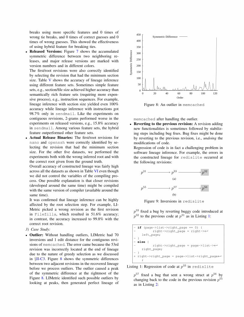
3) Handling Outliers: As an optional step, LIMetrichandles outliers in our recovered ordering, if any. SinceLIMetric constructs lineage in a greedy way, if one revisionis not selected mistakenly, that revision may not be selecteduntil the very last round. Suppose we have 5 revisions: p1,p2, p3, p4, and p5. If LIMetric falsely selects p3 as the nextrevision of p1 (p1 → p3) and SD(p3, p4) < SD(p3, p2), thenp4 will be chosen as the next revision (p1 → p3 → p4). Itis likely that SD(p4, p5) < SD(p4, p2) holds because p4 andp5 are neighboring revisions, and then p5 will be selected(p1 → p3 → p4 → p5). The probability of selecting p2 isgetting lower and lower if we have more revisions. At lastp2 is added as the last revision (p1 → p3 → p4 → p5 → p2)and becomes an outlier.

In order to detect outliers, LIMetric monitors the symmet-ric difference between every two adjacent pairs. An outliercan cause a peak of the symmetric difference (see Figure 8for an example). In our example, SD(p5, p2) is likely to behigher than the symmetric difference between other pairs.

If any possible outlier is identified by looking at apeak, then the possible outlier is moved either before orafter the closest revision where the symmetric difference isminimized. Suppose p3 is the closest revision to p2. LIMetriccompares SD(p1, p3) (the gap before the closest revision)with SD(p3, p4) (the gap after the closest revision), theninsert p2 to the bigger gap to minimize overall symmetricdifference. If SD(p3, p4) of neighboring revisions is smallerthan SD(p1, p3), we have p1 → p2 → p3 → p4 → p5.

4) Lineage Quality Metrics: We use dates of commithistories and version numbers as the ground truth of orderingG∗ = (N,A∗), and compare the recovered ordering byLIMetric G = (N,A) with the ground truth to measure

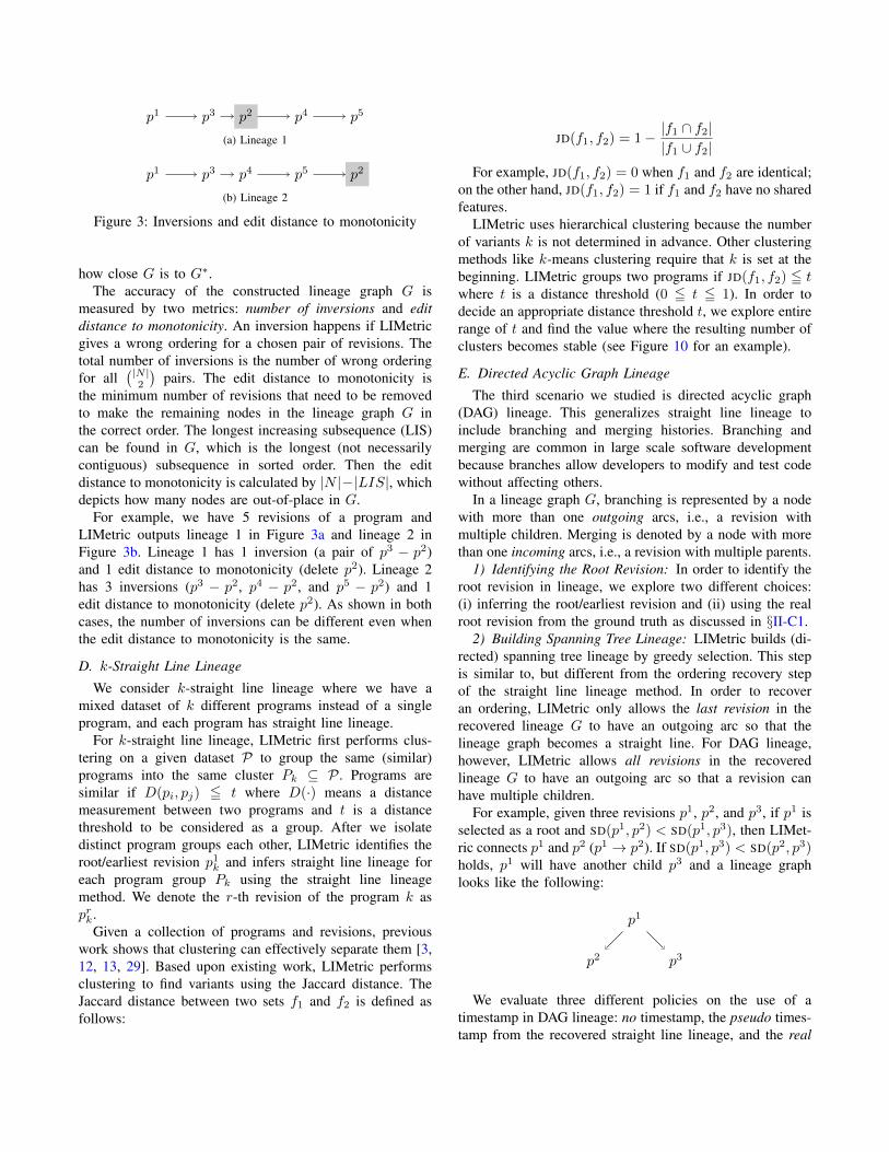
p1 p3 p2 p4 p5

(a) Lineage 1

p1 p3 p4 p5 p2

(b) Lineage 2

Figure 3: Inversions and edit distance to monotonicity

how close G is to G∗.The accuracy of the constructed lineage graph G is

measured by two metrics: number of inversions and editdistance to monotonicity. An inversion happens if LIMetricgives a wrong ordering for a chosen pair of revisions. Thetotal number of inversions is the number of wrong orderingfor all

(|N |2

)pairs. The edit distance to monotonicity is

the minimum number of revisions that need to be removedto make the remaining nodes in the lineage graph G inthe correct order. The longest increasing subsequence (LIS)can be found in G, which is the longest (not necessarilycontiguous) subsequence in sorted order. Then the editdistance to monotonicity is calculated by |N |−|LIS|, whichdepicts how many nodes are out-of-place in G.

For example, we have 5 revisions of a program andLIMetric outputs lineage 1 in Figure 3a and lineage 2 inFigure 3b. Lineage 1 has 1 inversion (a pair of p3 − p2)and 1 edit distance to monotonicity (delete p2). Lineage 2has 3 inversions (p3 − p2, p4 − p2, and p5 − p2) and 1edit distance to monotonicity (delete p2). As shown in bothcases, the number of inversions can be different even whenthe edit distance to monotonicity is the same.

D. k-Straight Line Lineage

We consider k-straight line lineage where we have amixed dataset of k different programs instead of a singleprogram, and each program has straight line lineage.

For k-straight line lineage, LIMetric first performs clus-tering on a given dataset P to group the same (similar)programs into the same cluster Pk ⊆ P . Programs aresimilar if D(pi, pj) 5 t where D(·) means a distancemeasurement between two programs and t is a distancethreshold to be considered as a group. After we isolatedistinct program groups each other, LIMetric identifies theroot/earliest revision p1k and infers straight line lineage foreach program group Pk using the straight line lineagemethod. We denote the r-th revision of the program k asprk.

Given a collection of programs and revisions, previouswork shows that clustering can effectively separate them [3,12, 13, 29]. Based upon existing work, LIMetric performsclustering to find variants using the Jaccard distance. TheJaccard distance between two sets f1 and f2 is defined asfollows:

JD(f1, f2) = 1− |f1 ∩ f2||f1 ∪ f2|

For example, JD(f1, f2) = 0 when f1 and f2 are identical;on the other hand, JD(f1, f2) = 1 if f1 and f2 have no sharedfeatures.

LIMetric uses hierarchical clustering because the numberof variants k is not determined in advance. Other clusteringmethods like k-means clustering require that k is set at thebeginning. LIMetric groups two programs if JD(f1, f2) 5 twhere t is a distance threshold (0 5 t 5 1). In order todecide an appropriate distance threshold t, we explore entirerange of t and find the value where the resulting number ofclusters becomes stable (see Figure 10 for an example).

E. Directed Acyclic Graph Lineage

The third scenario we studied is directed acyclic graph(DAG) lineage. This generalizes straight line lineage toinclude branching and merging histories. Branching andmerging are common in large scale software developmentbecause branches allow developers to modify and test codewithout affecting others.

In a lineage graph G, branching is represented by a nodewith more than one outgoing arcs, i.e., a revision withmultiple children. Merging is denoted by a node with morethan one incoming arcs, i.e., a revision with multiple parents.

1) Identifying the Root Revision: In order to identify theroot revision in lineage, we explore two different choices:(i) inferring the root/earliest revision and (ii) using the realroot revision from the ground truth as discussed in §II-C1.

2) Building Spanning Tree Lineage: LIMetric builds (di-rected) spanning tree lineage by greedy selection. This stepis similar to, but different from the ordering recovery stepof the straight line lineage method. In order to recoveran ordering, LIMetric only allows the last revision in therecovered lineage G to have an outgoing arc so that thelineage graph becomes a straight line. For DAG lineage,however, LIMetric allows all revisions in the recoveredlineage G to have an outgoing arc so that a revision canhave multiple children.

For example, given three revisions p1, p2, and p3, if p1 isselected as a root and SD(p1, p2) < SD(p1, p3), then LIMet-ric connects p1 and p2 (p1 → p2). If SD(p1, p3) < SD(p2, p3)holds, p1 will have another child p3 and a lineage graphlooks like the following:

p1

p2 p3

We evaluate three different policies on the use of atimestamp in DAG lineage: no timestamp, the pseudo times-tamp from the recovered straight line lineage, and the real

timestamp from the ground truth. Without a timestamp, therevision pr to be added to G is determined by the minimumsymmetric difference min{SD(pt, pr) : pt ∈ N̂ , pr ∈ N̂ c}where N̂ ⊆ N represents a set of nodes already insertedinto G and N̂ c denotes a complement of N̂ ; and an arc(pt, pr) is added. However, with the use of a timestamp, therevision pr ∈ N̂ c to be inserted is determined by the earliesttimestamp and an arc is drawn based upon the minimumsymmetric difference. In other words, we insert nodes inthe order of timestamps.

3) Adding Non-Tree Arcs: While building (directed)spanning tree lineage, LIMetric identifies branching pointsby allowing the revisions pt ∈ N̂ to have more than oneoutgoing arcs—revisions with multiple children. In order topinpoint merging points, LIMetric adds non-tree arcs alsoknown as cross arcs to the spanning tree lineage.

For every non-root node pi, LIMetric identifies a uniquefeature set ui that does not come from its parent pj , i.e., ui ={x : x ∈ f i and x 6∈ f j}. Then LIMetric examines if ui andfk extracted from pk ∈ N(k 6= i, j) have common features,and adds a non-tree arc from pk to pi, if any. Consequently,pi becomes a merging point of pj and pk and a lineage graphlooks like the following:

pj pk

pi

After adding non-tree arcs, LIMetric outputs DAG lineageshowing both branching and merging.

4) Lineage Quality Metrics: We propose measuring theaccuracy of the constructed DAG lineage graph by twometrics: number of LCA mismatches and average pairwisedistance to true LCA. Note that an inversion is a special caseof an LCA mismatch because querying the LCA of x and yin a straight line is the same as asking which one of x andy comes first.

We define SLCA(x, y) to be the set of LCAs of x andy because there can be multiple LCAs. For example, inFigure 4, SLCA(p4, p5) = {p2, p3} while SLCA(p6, p7) ={p4}. Given SLCA(x, y) in G and the true SLCA∗(x, y)

p1

p2 p3

p4 p5

p6 p7

Figure 4: Lowest common ancestors

in G∗, we can evaluate the correct LCA score of (x, y)C(SLCA(x, y), SLCA∗(x, y)) in the following four differentways.

(i) 1 point (correct) if SLCA(x, y) = SLCA∗(x, y)(ii) 1 point (correct) if SLCA(x, y) ⊆ SLCA∗(x, y)

(iii) 1 point (correct) if SLCA(x, y) ⊇ SLCA∗(x, y)(iv) 1− JD(SLCA(x, y), SLCA∗(x, y)) point

Then the number of LCA mismatches is

|N ×N | −∑

(x,y)∈N×N

C(SLCA(x, y), SLCA∗(x, y)).

The 1st policy is sound and complete, i.e., we only considerexact match of SLCA. However, even small errors can leadto a large number of LCA mismatches. The 2nd policy issound, i.e., every node in SLCA is indeed a true LCA (nofalse positive). Nonetheless, including any extra node willresult in a mismatch. The 3rd policy is complete, i.e., SLCAmust contain all true LCAs (no false negative). However,missing any true LCA will result in a mismatch. The 4thpolicy uses the Jaccard distance to measure dissimilaritybetween SLCA and SLCA∗. In our evaluation, LIMetricfollowed the 4th policy since it allows us to attain a morefine-grained measure.

In the case of an LCA mismatch, i.e., C(SLCA, SLCA∗) 6=1, we also propose a metric to measure the distance betweenthe true LCA(s) and the reported LCA(s). For example,if LIMetric falsely reports p5 as an LCA of p6 and p7

in Figure 4, then the pairwise distance to true LCA is 2(= distance between p4 and p5). Formally, let dist(u, v)represent the distance between nodes u and v in the groundtruth G∗. Given SLCA(x, y) and SLCA∗(x, y), we define thepairwise distance to true LCA D(SLCA(x, y), SLCA∗(x, y))to be ∑

(l,l∗)∈SLCA(x,y)×SLCA∗(x,y)

dist(l, l∗)|SLCA(x, y)× SLCA∗(x, y)|

and the average pairwise distance to true LCA to be∑(x,y)∈A′

D(SLCA(x, y), SLCA∗(x, y))

S,

where S equals to |{(x, y) ∈ N ×N s.t. C(SLCA(x, y),SLCA∗(x, y)) 6= 1}|.

III. IMPLEMENTATION

LIMetric is implemented using C (2.5 KLoC) andIDAPython plugin (100 LoC). We use the IDA Pro dis-assembler1 to disassemble binary programs and to identifybasic blocks. As discussed in §II-A, gcc -S output is usedto compensate the errors introduced at the disassemblingstep. For the scalability reason, we use feature hashingtechnique [13, 27] to encode extracted features into bit-vectors.

1http://www.hex-rays.com/products/ida/index.shtml

ExtractFeatures

PerformClustering

IdentifyRoot

Revision

ConstructLineage

[software] [k code bases] [lineage]

Figure 5: Software lineage inference overview

Let bv1 and bv2 denote two bit-vectors generated from f1and f2 using feature hashing. Then the symmetric differencein Equation 1 can be calculated by:

SDbv(bv1, bv2) = S(bv1 ⊗ bv2) (2)

where ⊗ denotes bitwise-XOR and S(·) means the numberof bits set to one. The use of fast bitwise operations on bit-vectors instead of slow set operations allows LIMetric toperform experiments with a number of variables quickly.

IV. EVALUATION

We systematically explored all the design spaces in Fig-ure 1 with a variety of datasets using LIMetric as depictedin Figure 5.

A. 1-Straight Line Lineage

1) Datasets: For 1-straight line lineage experiments, wehave collected three different kinds of datasets: contiguousrevisions, released versions, and actual release binary files.• Contiguous Revisions: Using a commit history from

a version control system, e.g., subversion and git, wedownloaded contiguous revisions of a program. Thetime gap between two adjacent commits varies a lot,from <10 minutes to more than a month. We excludedsome revisions which changed only comments becausethey did not affect the resulting binary programs.

Programs # revisions First rev Last rev

memcached 124 2008-10-14 2012-02-02

redis 158 2011-09-29 2012-03-28

redislite 89 2011-06-02 2012-01-18

Table I: Datasets of contiguous revisions

In order to set up idealized experiment environments,we compiled every revision with the same compilerand the same compiler options. In other words, weexcluded variations that can come from the use ofdifferent compilers.

• Released Versions: We downloaded only released ver-sions of a program meant to be distributed to end users.For example, Subversion maintains them under thetags folder. The difference with contiguous revisions

is that contiguous revisions may have program bugs(committed before testing) or experimental function-alities which would be excluded in released versions.In other words, released versions are more controlleddatasets. We also compiled source code with the samecompiler and the same compiling options for idealsettings.

Programs #releases

First release Last release

Ver Date Ver Date

grep 19 2.0 1993-05-22 2.11 2012-03-02

nano 114 0.7.4 2000-01-09 2.3.1 2011-05-10

redis 48 1.0 2009-09-03 2.4.10 2012-03-30

sendmail 38 8.10.0 2000-03-03 8.14.5 2011-05-15

openssh 52 2.0.0 2000-05-02 5.9p1 2011-09-06

Table II: Datasets of released versions

• Actual Release Binaries: We collected binary files (notsource code) of released versions from rpm or debpackage files. The difference is that we did not haveany control over the compiling process of the program,i.e., different programs may be compiled with differentversions of compilers and/or optimization options. Thisdataset is a representative of real-world scenarios wherewe do not have any information about developmentenvironments.

Programs #releases

First release Last release

Ver Date Ver Date

grep 37 2.0-3 2009-08-02 2.11-3 2012-04-17

nano 69 0.7.9-1 2000-01-24 2.2.6-1 2010-11-22

redis 39 0.094-1 2009-05-06 2.4.9-1 2012-03-26

sendmail 41 8.13.3-6 2005-03-12 8.14.4-2 2011-04-21

openssh 75 3.9p1-2 2005-03-12 5.9p1-5 2012-04-02

FileZilla 62 3.0.0 2007-09-13 3.5.3 2012-01-08

p7zip 32 0.91 2004-08-21 9.20.1 2011-03-16

Table III: Datasets of actual released binaries

2) Results: What selection of features provides the bestlineage graph with respect to the number of inversions and

200

205

210

215

220

225

230

235

240

245

250

0 20 40 60 80 100 120 1350

1400

1450

1500

1550

1600

1650

1700

File

Siz

e (K

B)

Cyc

lom

atic

Com

plex

ity

Revision

File SizeCyclomatic Complexity

(a) memcached

2550

2600

2650

2700

2750

2800

2850

0 20 40 60 80 100 120 140 9000

9200

9400

9600

9800

10000

10200

10400

File

Siz

e (K

B)

Cyc

lom

atic

Com

plex

ity

Revision

File SizeCyclomatic Complexity

(b) redis

180

190

200

210

220

230

240

250

260

270

280

290

0 10 20 30 40 50 60 70 80 1100

1200

1300

1400

1500

1600

1700

1800

1900

2000

File

Siz

e (K

B)

Cyc

lom

atic

Com

plex

ity

Revision

File SizeCyclomatic Complexity

(c) redislite

Figure 6: File size and complexity for contiguous revisions

memcached redis redislite

# Inversion ED # Ties # Inversion ED # Ties # Inversion ED # Ties

Section size 357 (95.3%) 48 34 (12/22) 57 (99.5%) 28 31 (13/18) 47 (98.8%) 19 20 (11/9)

File size 171 (97.8%) 39 13 (9/4) 93 (99.3%) 36 31 (17/14) 50 (98.7%) 21 9 (3/6)

2-grams 38 (99.5%) 17 2 (2/0) 783 (93.7%) 55 21 (10/11) 134 (96.6%) 21 3 (1/2)

4-grams 24 (99.7%) 11 0 (0/0) 50 (99.6%) 25 0 (0/0) 45 (98.9%) 17 0 (0/0)

8-grams 92 (98.8%) 15 0 (0/0) 30 (99.8%) 17 1 (1/0) 46 (98.8%) 18 0 (0/0)

16-grams 60 (99.2%) 14 0 (0/0) 40 (99.7%) 21 0 (0/0) 131 (96.7%) 19 0 (0/0)

Instructions 233 (96.9%) 31 6 (2/4) 304 (97.6%) 58 6 (4/2) 208 (94.7%) 27 7 (2/5)

Mnemonics 75 (99.0%) 6 9 (4/5) 26 (99.8%) 18 29 (15/14) 13 (99.7%) 5 8 (6/2)

Normalized 75 (99.0%) 5 10 (6/4) 26 (99.8%) 17 30 (17/13) 7 (99.8%) 7 10 (5/5)

Hybrid 0 (100%) 0 0 (10/0, 0/0) 15 (99.9%) 8 0 (26/4, 0/0) 3 (99.9%) 3 0 (8/1, 0/0)

Table IV: Lineage accuracy for contiguous revisions (Percentage in inversion columns denotes accuracy.)

the edit distance to monotonicity? We evaluated differentfeatures sets on diverse datasets.• Contiguous Revisions: In order to identify the first

revision of each program, code complexity and codesize of every revision were measured. As shown inFigure 6, both file size and cyclomatic complexitygenerally increased as new revisions were released.For these three datasets, the first/root revisions werecorrectly identified by selecting the revision that hadthe minimum file size and cyclomatic complexity.Lineage for each program was constructed as describedin §II-C. The accuracy results including the number ofinversions, the edit distance to monotonicity, and thenumber of ties are shown in Table IV. The numbersin parentheses in tie columns denote the number ofcorrect/wrong random guessing in case of ties.Section/file size achieved high accuracy from 95.3% to99.5%. However, there were many ties, which mightincrease/decrease the accuracy depending on randomguessing choices.n-grams over byte sequences generally achieved better

accuracy; however, 2-grams (small size of n) and 16-grams (big size of n) were relatively unreliable features,e.g., 6.3% inversion error in redis and 3.3% inversionerror in redislite. In our experiments, n=4 bytesworked reasonably well for these three datasets.The usage of disassembly instructions had up to 5.3%inversion error in redislite. Most errors camefrom syntactical differences, e.g., changes in offsetsand jump target addresses. After normalizing operands,instruction mnemonics with operands types decreasedthe errors substantially, e.g., from 5.3% to 0.3%.With additional normalization, normalized instructionmnemonics with operands types achieved the same orbetter accuracy. Note that more normalized features canresult in better or worse accuracy because there may bemore ties where random guessing is involved.In order to break ties, more specific features were usedin the hybrid feature. Regarding the hybrid feature,correct/wrong tie breaks using specific features are alsopresented. For example, 10/0, 0/0 at the hybrid featurerow for memcached means 10 times of correct tie

0

1000

2000

3000

4000

5000

6000

7000

8000

9000

01/01/1996 01/01/2000 01/01/2004 01/01/2008 01/01/2012

Acc

umul

ated

Sym

met

ric

Dif

fere

nce

Date

2.0

2.22.3

2.4

2.5

2.6

2.72.82.92.10

2.11

(a) grep

0

5000

10000

15000

20000

25000

01/01/02 01/01/04 01/01/06 01/01/08 01/01/10A

ccum

ulat

ed S

ymm

etri

c D

iffe

renc

e

Date

0.7.40.8.00.9.0

1.0.01.1.0

1.2.01.3.0

2.0.02.1.0

2.2.0 2.3.0

(b) nano

0

2000

4000

6000

8000

10000

12000

14000

01/01/10 01/01/11 01/01/12

Acc

umul

ated

Sym

met

ric

Dif

fere

nce

Date

1.0

1.2.0

1.3.6

2.0.0

2.2.0

2.4.0

(c) redis

0

2000

4000

6000

8000

10000

12000

14000

16000

18000

01/01/02 01/01/04 01/01/06 01/01/08 01/01/10

Acc

umul

ated

Sym

met

ric

Dif

fere

nce

Date

8.10.08.11.0

8.12.0

8.13.0

8.14.0

(d) sendmail

0

2000

4000

6000

8000

10000

12000

14000

16000

01/01/02 01/01/04 01/01/06 01/01/08 01/01/10

Acc

umul

ated

Sym

met

ric

Dif

fere

nce

Date

2.0.0beta1

3.0p1

4.0p1

5.0p1

(e) openssh

Figure 7: Releases and the accumulated symmetric difference of released versions

grep nano redis sendmail openssh

# Inversion ED # Inversion ED # Inversion ED # Inversion ED # Inversion ED

Section size 21 (87.7%) 6 86 (98.7%) 26 10 (99.1%) 6 0 (100%) 0 42 (96.8%) 12

File size 4 (97.7%) 4 59 (99.1%) 23 11 (99.0%) 7 24 (96.6%) 10 18 (98.6%) 9

2-grams 29 (83.0%) 8 26 (99.6%) 9 324 (70.0%) 29 592 (15.8%) 30 695 (47.6%) 39

4-grams 3 (98.3%) 3 10 (99.8%) 6 6 (99.4%) 3 1 (99.9%) 1 5 (99.6%) 5

8-grams 2 (98.8%) 2 8 (99.9%) 5 17 (98.4%) 5 1 (99.9%) 1 5 (99.6%) 5

16-grams 2 (98.8%) 2 16 (99.8%) 7 15 (98.6%) 4 1 (99.9%) 1 5 (99.6%) 5

Instructions 38 (77.8%) 5 15 (99.8%) 10 29 (97.3%) 11 9 (98.7%) 5 14 (98.9%) 8

Mnemonics 0 (100%) 0 6 (99.9%) 5 5 (99.5%) 4 5 (99.3%) 1 2 (99.9%) 2

Normalized 0 (100%) 0 4 (99.9%) 4 5 (99.5%) 4 5 (99.3%) 1 3 (99.8%) 3

Hybrid 0 (100%) 0 1 (99.9%) 1 1 (99.9%) 1 5 (99.3%) 1 3 (99.8%) 3

Table V: Lineage accuracy for released versions (Percentage in inversion columns denotes accuracy.)

breaks using more specific features and 0 times ofwrong tie breaks, and 0 times of correct guesses and 0times of wrong guesses. This showed the effectivenessof using hybrid feature for breaking ties.

• Released Versions: Figure 7 shows the accumulatedsymmetric difference between two neighboring re-leases, and major release versions are marked withversion numbers and in different colors.The first/root revisions were also correctly identifiedby selecting the revision that had the minimum sectionsize. Table V shows the accuracy of lineage inferenceusing different feature sets. Sometimes simple featuresets, e.g., section/file size achieved higher accuracy thansemantically rich feature sets (requiring more expen-sive process), e.g., instruction sequences. For example,lineage inference with section size yielded even 100%accuracy while lineage inference with instructions got98.7% only in sendmail. Like the experiments oncontiguous revisions, 2-grams performed worse in theexperiments on released versions, e.g., 15.8% accuracyin sendmail. Among various feature sets, the hybridfeature outperformed other feature sets.

• Actual Release Binaries: The first/root revisions fornano and openssh were correctly identified by se-lecting the revision that had the minimum sectionsize. For the other five datasets, we performed theexperiments both with the wrong inferred root and withthe correct root given from the ground truth.Overall accuracy of constructed lineage was fairly highacross all the datasets as shown in Table VI even thoughwe did not control the variables of the compiling pro-cess. One possible explanation is that closer revisions(developed around the same time) might be compiledwith the same version of compiler (available around thesame time).It was confirmed that lineage inference can be highlyaffected by the root selection step. For example, LI-Metric picked a wrong revision as the first revisionin FileZilla, which resulted in 51.6% accuracy;in contrast, the accuracy increased to 99.8% with thecorrect root revision.

3) Case Study:• Outlier: Without handling outliers, LIMetric had 70

inversions and 1 edit distance for the contiguous revi-sions of memcached. The error came because the 53rdrevision was incorrectly located at the end of lineagedue to the nature of greedy selection as we discussedin §II-C3. Figure 8 shows the symmetric differencesbetween two adjacent revisions in the recovered lineagebefore we process outliers. The outlier caused a peakof the symmetric difference at the rightmost of theFigure 8. LIMetric identified such possible outliers bylooking at peaks, then generated perfect lineage of

0

50

100

150

200

250

300

350

400

450

0 20 40 60 80 100 120

Sym

met

ric

Dif

fere

nce

Order

Symmetric Difference

Figure 8: An outlier in memcached

memcached after handling the outlier.• Reverting to the previous revision: A revision adding

new functionalities is sometimes followed by stabiliz-ing steps including bug fixes. Bug fixes might be doneby reverting to the previous revision, i.e., undoing themodifications of code.Regression of code is in fact a challenging problem insoftware lineage inference. For example, the errors inthe constructed lineage for redislite occurred atthe following revisions:

p31 p33 p32

(a)

p55 p57 p56

(b)

Figure 9: Inversions in redislite

p33 fixed a bug by reverting buggy code introduced atp32 to the previous code at p31 as in Listing 1:

- if (page->list->right_page == 0) {- right->right_page = right->←↩

left_page;- }- else {- right->right_page = page->list->←↩

right_page;- }+ right->right_page = page->list->right_page←↩

;

Listing 1: Regression of code at p33 in redislite

p57 fixed a bug that sent a wrong struct at p56 bychanging back to the code in the previous revision p55

as in Listing 2:

grep nano redis openssh

Inferred root Real root Inferred root Real root

# Inversion ED # Inversion ED # Inversion ED # Inversion ED # Inversion ED # Inversion ED

Section size 57 (91.4%) 17 75 (88.7%) 18 104 (95.6%) 22 32 (95.7%) 12 35 (95.3%) 15 235 (91.5%) 34

File size 38 (94.3%) 13 36 (94.6%) 12 144 (93.9%) 27 33 (95.6%) 12 37 (95.0%) 12 274 (90.1%) 32

2-grams 148 (77.8%) 22 74 (88.9%) 13 411 (82.5%) 30 333 (55.1%) 25 357 (51.8%) 24 2041 (26.5%) 64

4-grams 30 (95.5%) 11 12 (98.2%) 8 19 (99.2%) 8 50 (93.3%) 11 45 (93.9%) 10 398 (85.7%) 19

8-grams 39 (94.1%) 13 24 (96.4%) 10 10 (99.6%) 5 12 (98.4%) 12 29 (96.1%) 12 146 (94.7%) 22

16-grams 62 (90.7%) 17 54 (91.9%) 15 12 (99.5%) 6 28 (96.2%) 10 23 (96.9%) 9 300 (96.9%) 25

Instructions 88 (86.8%) 18 63 (90.5%) 13 68 (97.1%) 12 30 (96.0%) 10 27 (96.4%) 10 295 (89.2%) 30

Mnemonics 32 (95.2%) 13 13 (98.1%) 9 2 (99.9%) 2 28 (96.2%) 9 24 (96.8%) 8 396 (85.7%) 22

Normalized 25 (96.3%) 10 7 (99.0%) 6 5 (99.8%) 4 28 (96.2%) 9 25 (96.6%) 9 397 (85.7%) 22

Hybrid 26 (96.1%) 10 9 (98.7%) 7 4 (99.8%) 3 30 (96.0%) 11 26 (96.5%) 10 398 (85.7%) 23

sendmail FileZilla p7zip

Inferred root Real root Inferred root Real root Inferred root Real root

# Inversion ED # Inversion ED # Inversion ED # Inversion ED # Inversion ED # Inversion ED

Section size 121 (85.2%) 24 110 (86.6%) 21 492 (74.0%) 26 489 (74.1%) 25 208 (58.1%) 20 284 (42.7%) 21

File size 123 (85.0%) 22 131 (84.0%) 23 987 (47.8%) 35 840 (55.6%) 45 200 (59.7%) 19 292 (41.1%) 22

2-grams 298 (63.7%) 24 219 (73.3%) 24 1176 (37.8%) 52 1099 (41.9%) 51 314 (36.7%) 26 321 (35.3%) 25

4-grams 184 (77.6%) 16 141 (82.8%) 15 920 (51.4%) 28 8 (99.6%) 6 200 (59.7%) 16 12 (97.6%) 6

8-grams 131 (84.0%) 20 104 (87.3%) 18 765 (59.6%) 24 5 (99.7%) 5 197 (60.3%) 16 67 (86.5%) 9

16-grams 32 (96.1%) 15 19 (97.7%) 11 766 (59.5%) 23 3 (99.8%) 3 159 (67.9%) 12 47 (90.5%) 9

Instructions 220 (73.2%) 19 176 (78.5%) 19 768 (59.4%) 24 800 (57.7%) 27 196 (60.5%) 18 138 (72.2%) 15

Mnemonics 185 (77.4%) 20 138 (83.2%) 18 916 (51.6%) 27 5 (99.7%) 5 189 (61.9%) 12 57 (88.5%) 5

Normalized 153 (81.3%) 24 136 (83.4%) 17 916 (51.6%) 27 3 (99.8%) 3 189 (61.9%) 12 57 (88.5%) 5

Hybrid 151 (81.6%) 24 137 (83.3%) 18 915 (51.6%) 26 3 (99.8%) 3 189 (61.9%) 12 57 (88.5%) 5

Table VI: Lineage accuracy for actual release binaries (Percentage in inversion columns denotes accuracy.)

- status = redislite_insert_key(_cs, page->←↩page, str, length, 1, ←↩REDISLITE_PAGE_TYPE_FIRST);

+ status = redislite_insert_key(_cs, page, ←↩str, length, 1, ←↩REDISLITE_PAGE_TYPE_FIRST);

Listing 2: Regression of code at p57 in redislite

The code was reverted to the previous revision sothat SD(p31, p33) < SD(p31, p32) and SD(p55, p57) <SD(p55, p56). As a result, inversions happened at p32

and p56. We argue that unless we build a precisemodel describing the developers’ reverting activity, noreasonable algorithm may be able to construct the samelineage as the ground truth. Rather, the constructedlineage can be a representation of more “practical”evolutionary relationships.

Our data indicates that the hybrid feature can achieve over99% accuracy in idealized settings, and over 83% accuracyon real-world binaries. Using similar techniques, e.g., for

malware, one cannot expect to do much better.

B. k-Straight Line Lineage

Does having multiple mixed k-straight line lineage soft-ware affect results? For 2 straight line of lineage, we mixedmemcached and redislite in that both programs havethe same functionality, similar code section sizes, and areasonable number of revisions. Figure 10 shows the re-sulting number of clusters with various similarity threshold.From 0.5 to 0.8 similarity threshold, the resulting numberof clusters were 2. This means LIMetric can first performclustering to divide the dataset into two groups, then buildstraight line lineage for each group.

The resulting number of clusters of the mixed datasetof 3 programs including memcached, redislite, andredis became stabilized to 3 from 0.5 to 0.8 similaritythreshold, which means they were successfully clustered forthe subsequent straight line lineage building process.

0

10

20

30

40

50

60

70

80

90

100

0.5 0.6 0.7 0.8 0.9 1

Num

ber

of C

lust

ers

Similarity Threshold

3 sets of programs2 sets of programs

Figure 10: Number of clusters from 2 and 3 sets of programs

C. Directed Acyclic Graph Lineage

1) Datasets: We have collected 10 datasets for directedacyclic graph lineage experiments from github2. We usedgithub because we know when a project is forked from anetwork graph showing the development history as a graphincluding branching and merging.

We downloaded DAG-like revisions that had multipletimes of branching and merging histories, and compiled withthe same compilers and optimization options.

Programs # revisions First rev Last rev

http-parser 55 2010-11-05 2012-07-27

libgit2 61 2012-06-25 2012-07-17

redis 98 2010-04-29 2010-06-04

redislite 97 2011-04-19 2011-06-12

shell-fm 107 2008-10-01 2012-06-26

stud 73 2011-06-09 2012-06-01

tig 58 2006-06-06 2007-06-19

uzbl 73 2011-08-07 2012-07-01

webdis 96 2011-01-01 2012-07-20

yajl 62 2010-07-21 2011-12-19

Table VII: Datasets of DAG lineage

2) Results: We set two policies for DAG lineage experi-ments: the use of timestamp (none/pseudo/real) and the useof the real root (none/real). The real timestamp implies thereal root so that we explored 3× 2− 1 = 5 different setups.We used hybrid feature sets for DAG lineage experimentsin that hybrid feature sets were demonstrated to attain thebest accuracy in constructing straight line lineage.

Without having any prior knowledge, as described in Ta-ble VIII, LIMetric achieved from 60.8% to 89.5% accuracy

2https://github.com/

p17 p18 p19 p20 p21 p22 p23

(a) Ground truth

p17 p18 p19 p20

p21 p22 p23

(b) Constructed lineage

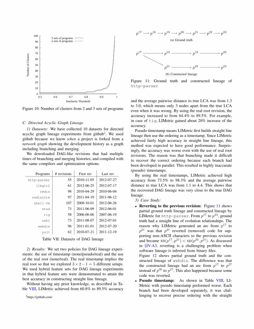
Figure 11: Ground truth and constructed lineage ofhttp-parser

and the average pairwise distance to true LCA was from 1.3to 3.0, which means only 3 nodes apart from the true LCAeven when it was wrong. By using the real root revision, theaccuracy increased to from 64.4% to 89.5%. For example,in case of tig, LIMetric gained about 20% increase of theaccuracy.

Pseudo timestamp means LIMetric first builds straight linelineage then use the ordering as a timestamp. Since LIMetricachieved fairly high accuracy in straight line lineage, thismethod was expected to have good performance. Surpris-ingly, the accuracy was worse even with the use of real rootrevisions. The reason was that branching made it difficultto recover the correct ordering because each branch hadbeen developed in parallel. This resulted in highly inaccurate(pseudo) timestamps.

By using the real timestamps, LIMetric achieved highaccuracy from 73.5% to 98.3% and the average pairwisedistance to true LCA was from 1.1 to 4.4. This shows thatthe recovered DAG lineage was very close to the true DAGlineage.

3) Case Study:• Reverting to the previous revision: Figure 11 shows

partial ground truth lineage and constructed lineage byLIMetric for http-parser. From p17 to p23, groundtruth had a straight line of evolution relationships. Thereason why LIMetric generated an arc from p17 top21 was that p21 reverted (removed) code for sup-porting non-ASCII characters to the previous revisionand became SD(p17, p21) < SD(p20, p21). As discussedin §IV-A3, reverting is a challenging problem whensoftware lineage is inferred from binary files.Figure 12 shows partial ground truth and the con-structed lineage of webdis. The difference was thatthe constructed lineage had an arc from p17 to p27

instead of p26 to p27. This also happened because somecode was reverted.

• Pseudo timestamp: As shown in Table VIII, LI-Metric with pseudo timestamp performed worse. Eachbranch had been developed separately, it was chal-lenging to recover precise ordering with the straight

Policies http-parser libgit2 redis redislite shell-fmTimestamp

RealRoot

LCAMismatch

AvgDist

LCAMismatch

AvgDist

LCAMismatch

AvgDist

LCAMismatch

AvgDist

LCAMismatch

AvgDist

- - 582 (60.8%) 1.8 439 (76.0%) 2.8 613 (87.1%) 1.4 524 (88.8%) 2.0 1619 (71.5%) 2.2

-√

528 (64.4%) 1.9 439 (76.0%) 2.8 613 (87.1%) 1.4 507 (89.1%) 2.0 1524 (73.1%) 2.8

Pseudo - 653 (56.0%) 2.2 535 (70.8%) 5.1 706 (85.2%) 1.9 978 (79.0%) 5.0 1893 (66.6%) 2.0

Pseudo√

599 (59.7%) 2.3 535 (70.8%) 5.1 706 (85.2%) 1.9 627 (86.5%) 1.7 1555 (72.6%) 3.1

Real√

394 (73.5%) 2.9 285 (84.4%) 2.3 485 (89.8%) 4.4 315 (93.2%) 1.1 1391 (75.5%) 2.2

Policies stud tig uzbl webdis yajlTimestamp

RealRoot

LCAMismatch

AvgDist

LCAMismatch

AvgDist

LCAMismatch

AvgDist

LCAMismatch

AvgDist

LCAMismatch

AvgDist

- - 901 (65.7%) 1.5 552 (66.6%) 2.6 584 (77.8%) 2.2 479 (89.5%) 1.3 479 (74.7%) 3.0

-√

878 (66.6%) 1.5 225 (86.4%) 1.4 331 (87.4%) 2.6 479 (89.5%) 1.3 479 (74.7%) 3.0

Pseudo - 1307 (50.3%) 7.2 824 (50.2%) 5.8 1342 (48.9%) 7.3 1533 (66.4%) 14.4 769 (59.3%) 5.2

Pseudo√

1340 (49.0%) 7.1 524 (68.3%) 7.1 964 (63.3%) 8.8 1533 (66.4%) 14.4 751 (60.3%) 5.3

Real√

389 (85.2%) 1.2 28 (98.3%) 2.0 211 (92.0%) 1.2 256 (94.4%) 1.4 325 (82.8%) 1.9

Table VIII: Lineage accuracy for directed acyclic graph lineage (Percentage in LCA Mismatch columns denotes accuracy.)

p17 p19 p20 p21

p22

p23

p24

p25

p26 p27 p28

p29

(a) Ground truth

p17 p19 p20 p21

p22

p23

p24

p25

p26

p27 p28

p29

(b) Constructed lineage

Figure 12: Ground truth and constructed lineage of webdis

line lineage method. For example, Figure 13 showsthe partial ground truth and the constructed lin-eage by LIMetric for uzbl with pseudo times-tamp. LIMetric without timestamp successfully re-covered the ground truth lineage. However, the useof pseudo timestamp resulted in poor performance.The recovered ordering, i.e., pseudo timestamp wasp22, p40, p41, p42, p43, p23, p29, p30, p35, p36. Due to theimprecise timestamp, the derivation relationships in theconstructed lineage was not accurate.

V. DISCUSSION

In many open source projects and malware, code sizeusually grows over time [7, 28]. In other words, addition

p22 p23 p29 p30 p35 p36

p40 p41 p42 p43

(a) Ground truth

p22 p23 p29 p30 p35 p36

p40 p41 p42 p43

(b) Constructed lineage

Figure 13: Ground truth and constructed lineage of uzbl

of new code is preferred to deletion of existing code. Thisalso holds in our datasets except for major changes followedby minor cleanups. Differentiating the costs of addition anddeletion helps us to decide a direction of derivation. Supposea deletion cost is 2 and an addition cost is 1, i.e., a deletionis a twice expensive operation. Program pi has a feature setfi = {m1,m2,m3}, and program pj contains a feature setfj = {m1,m2,m4,m5}. A direction of evolution pi → pjhas a distance of 4 (=deletion of m3 and addition of m4 andm5). On the other hand, a direction of evolution pj → pihas a distance of 5 (=deletion of m4 and m5 and additionof m3). Consequently, pi → pj is a more plausible scenario.

We evaluated LIMetric with a deletion cost of 2 and anaddition cost of 1 with 10 DAG lineage datasets. Overallaverage accuracy remained almost the same, e.g., from75.74% to 75.28%. One possible reason was that one linemodification of source code would result in a deletion ofa basic block (feature) and an addition of a basic block

(feature), i.e., 1 modification = 1 deletion + 1 addition. Weleave it as a future work to distinguish a modification witha deletion and an addition.

Correct software lineage inference on a revision historymay not correspond with software release date lineage. Forexample, as shown in Figure 7b, a development branchof nano-1.3 and a stable branch of nano-1.2 aredeveloped in parallel. In straight line lineage, LIMetric inferssoftware lineage consistent with a revision history.

In our experiments, we used the symmetric difference as adistance metric. Other distance metrics can be considered asalternatives. For example, the Jaccard distance can be usedto calculate dissimilarity between two feature sets. However,the downside of the Jaccard distance is that the same amountof code change can yield different distances depending onthe size of feature sets, and the Jaccard distance does notindicate which features are added or deleted unlike thesymmetric difference.

VI. RELATED WORK

Existing research analyzed open source projects [28] andLinux kernel [10] to understand evolutionary relationshipamong programs, and studied the security implication ofsoftware evolution on known vulnerabilities in Firefox [21].Empirical study was performed to evaluate the effects ofbranching in software development on software quality withWindows Vista and Windows 7 [26].

In order to describe evolutionary relationships amongmalware, empirical study on malware metadata includingtext descriptions and dates collected by an anti-virus vendorwas performed [11], phylogeny of remote code injectionexploits was constructed [20], and phylogeny models weregenerated using n-perms of code [14]. Researchers usedderivation relationships among malware to find new variantsof well known malware [8].

There have been many approaches to abstract binaryprograms. Syntax-based methods identifies code sections ina program and extracts n-grams features on byte sequencesof program code, e.g., [13, 14, 16, 25]. Static analysismethods translates machine code into assembly code anduse instructions [15, 24, 29] and basic blocks [9]. Dynamicanalysis methods collect information about binary programsby monitoring program executions at run time [4, 23].

VII. CONCLUSION

In this paper, we systematically explored the entire designspace in software lineage inference. We built LIMetric tocontrol a number of variables and performed over 400 differ-ent experiments on large scale real-world programs—1,777releases for a combined 110 years of development history.We built software lineage on two types of lineage: straightline lineage and directed acyclic graph (DAG) lineage.We also proposed four metrics to measure lineage quality:number of inversions and edit distance to monotonicity for

straight line lineage, and number of LCA mismatches andaverage pairwise distance to true LCA for DAG lineage.We showed that LIMetric effectively extracted softwareevolutionary relationships among binary programs with highaccuracy.

REFERENCES

[1] DARPA-BAA-10-36, Cyber Genome Program. https://www.fbo.gov/spg/ODA/DARPA/CMO/DARPA-BAA-10-36/listing.html. Page checked 8/5/2012.

[2] Symantec internet security threat report. http://www.symantec.com/threatreport/. URL checked 8/5/2012.

[3] zynamics BinDiff. http://www.zynamics.com/bindiff.html.Page checked 8/5/2012.

[4] U. Bayer, P. M. Comparetti, C. Hlauschek, C. Kruegel, andE. Kirda. Scalable, behavior-based malware clustering. InProceedings of the Network and Distributed System SecuritySymposium, 2009.

[5] L. A. Belady and M. M. Lehman. A model of large programdevelopment. IBM Systems Journal, 15(3):225–252, Sept.1976.

[6] M. A. Bender, M. Farach-Colton, G. Pemmasani, S. Skiena,and P. Sumazin. Lowest common ancestors in trees anddirected acyclic graphs. Journal of Algorithms, 57(2):75–94,Nov. 2005.

[7] F. de la Cuadra. The geneology of malware. Network Security,(April):17–20, 2007.

[8] T. Dumitras and I. Neamtiu. Experimental challenges in cybersecurity: a story of provenance and lineage for malware. InCyber security experimentation and test, 2011.

[9] H. Flake. Structural comparison of executable objects. In Pro-ceedings of the IEEE Conference on Detection of Intrusions,Malware, and Vulnerability Assessment, 2004.

[10] M. W. Godfrey and Q. Tu. Evolution in open source software:A case study. In Proceedings of the International Conferenceon Software Maintenance, 2000.

[11] A. Gupta, P. Kuppili, A. Akella, and P. Barford. An empiricalstudy of malware evolution. In International CommunicationSystems and Networks and Workshops, pages 1–10, Jan. 2009.

[12] X. Hu, T. cker Chiueh, and K. G. Shin. Large-scale malwareindexing using function call graphs. In Proceedings of theACM Conference on Computer and Communications Security,2009.

[13] J. Jang, D. Brumley, and S. Venkataraman. BitShred: featurehashing malware for scalable triage and semantic analysis.In Proceedings of the ACM Conference on Computer andCommunications Security, 2011.

[14] M. E. Karim, A. Walenstein, A. Lakhotia, and L. Parida.Malware phylogeny generation using permutations of code.Journal in Computer Virology, 1:13–23, Sept. 2005.

[15] W. M. Khoo and P. Lio. Unity in diversity: Phylogenetic-inspired techniques for reverse engineering and detection ofmalware families. In SysSec Workshop, pages 3–10, July2011.

[16] J. Z. Kolter and M. A. Maloof. Learning to detect andclassify malicious executables in the wild. Journal of MachineLearning Research, 7:2721–2744, Dec. 2006.

[17] C. Kruegel, W. Robertson, F. Valeur, and G. Vigna. Static

disassembly of obfuscated binaries. In Proceedings of theUSENIX Security Symposium, 2004.

[18] M. M. Lehman and J. F. Ramil. Rules and tools for softwareevolution planning and management. Annals of SoftwareEngineering, 11(1):15–44, Nov. 2001.

[19] C. Linn and S. Debray. Obfuscation of executable code toimprove resistance to static disassembly. In Proceedings of theACM Conference on Computer and Communications Security,2003.

[20] J. Ma, J. Dunagan, H. J. Wang, S. Savage, and G. M. Voelker.Finding diversity in remote code injection exploits. In ACMSIGCOMM on Internet Measurement, page 53, 2006.

[21] F. Massacci, S. Neuhaus, and V. H. Nguyen. After-life vulner-abilities: a study on firefox evolution, its vulnerabilities, andfixes. In Proceedings of the Third international conferenceon Engineering secure software and systems, pages 195–208,2011.

[22] T. J. McCabe. A complexity measure. IEEE Transactions onSoftware Engineering, SE-2(4):308–320, Dec. 1976.

[23] K. Rieck, P. Trinius, C. Willems, and T. Holz. Automaticanalysis of malware behavior using machine learning. Journalof Computer Security, 19(4):639–668, 2011.

[24] A. Sæ bjørnsen, J. Willcock, T. Panas, D. Quinlan, and Z. Su.Detecting code clones in binary executables. In Internationalsymposium on Software testing and analysis, page 117, 2009.

[25] S. Schleimer, D. Wilkerson, and A. Aiken. Winnowing: Localalgorithms for document fingerprinting. In Proceedings of theACM SIGMOD/PODS Conference, 2003.

[26] E. Shihab, C. Bird, and T. Zimmermann. The effect ofbranching strategies on software quality. In ACM/IEEEInternational Symposium on Empirical Software Engineeringand Measurement, 2012.

[27] K. Weinberger, A. Dasgupta, J. Langford, A. Smola, andJ. Attenberg. Feature hashing for large scale multitasklearning. In International Conference on Machine Learning,2009.

[28] G. Xie, J. Chen, and I. Neamtiu. Towards a better understand-ing of software evolution: An empirical study on open sourcesoftware. Proceedings of the IEEE International Conferenceon Software Maintenance, pages 51–60, Sept. 2009.

[29] Y. Ye, T. Li, Y. Chen, and Q. Jiang. Automatic malwarecategorization using cluster ensemble. In ACM SIGKDDinternational conference on Knowledge discovery and datamining, pages 95–104, 2010.