Towards an Extension of the ����� � Model forTransitional Flows

A. SveningssonDepartment of Thermo and Fluid Dynamics,

Chalmers University of Technology,

SE-412 96 Gothenburg, Sweden

October 7, 2006

Abstract

In part, this study investigates the performance of the turbulence model of Waltersand Leylek (2004) in the flow over a flat plate under the influence of a disturbedfreestream. The most important feature of the model is that is solves an equationfor a laminar kinetic energy, which is coupled to a typical ��� model, to improvethe performance in transitional flows. The model is shown to be very sensitive tothe prescribed freestream turbulence length scale.

The study also describes the initial steps towards coupling the laminar kineticenergy transition modelling approach, suggested by Walters and Leylek (2004),to the � ����� turbulence model in an effort to improve the ������� model’s perfor-mance in transitional flow regimes. This coupling requires modifications of the� � �� model but the intention is that the new model should retain the properties ofthe original model in fully turbulent boundary layers and that the additional lam-inar kinetic energy equation should make the predictions in transitional boundarylayers more reliable.

Finally, in an initial numerical study some potential pitfalls when modellingthe flat plate flow are analyzed. It is shown that the predicted transitional behaviorobtained with the simplified, as compared with the experimental set-up, numericaldomain used in this study may be directly compared with measurements.

1

1 Introduction

With the last decades of intense research in turbulence modelling statistical de-scriptions of turbulence are about to mature. Today closures exist that are ableto provide accurate predictions of turbulence effects on the mean flow character-istics given that the mean flow itself is not too complicated. However, there isone phenomenon that can cause the most advanced turbulence model to fail inthe, seemingly, most straightforward flows to compute, e.g. flow over a flat plate.This phenomenon is the transition of a laminar boundary layer into a turbulentstate. With the improvements in turbulence modelling the inability to accountfor transitional effects has become more pronounced. The interest in developingmethods aimed at extending the applicability of turbulence models to include alsotransitional flows has therefore grown.

The present study deals with laminar to turbulence transition of boundary lay-ers due to elevated levels of freestream disturbances – so called bypass transition.The other two types of transition, natural transition and transition preceded byseparation, will at present not be included in the model framework developed inthe following sections. The reasons why bypass transition is considered are thatthe mechanism behind it is rather well suited for a statistical description, i.e. thereis a possibility that the phenomenon can be sufficiently accurately modelled with astandard RANS-based approach, and that bypass transition is commonly encoun-tered in gas turbine design, especially in the high pressure turbine where largelevels of freestream disturbances exist.

In bypass transition freestream disturbances penetrate the boundary layer andinduce low frequency fluctuations, primarily in the streamwise velocity compo-nent, � � . The fluctuations appear as long streamwise streaks within the boundarylayer and after an initial growth some of the streaks eventually collapse to formso called turbulent spots. Thus, most stages in the natural transition route to tur-bulence are bypassed and the boundary layer transitions earlier than the boundarylayer beneath an undisturbed freestream.

Much of the detailed physics behind bypass transition is still unknown. In aneffort to provide the data necessary to depict the interaction of freestream turbu-lence with a laminar boundary layer Jacobs and Durbin (2001) performed a DNSof a flat plate flow in an environment of elevated turbulence intensity,

���������%.

Their results suggest that low frequency perturbations in the freestream are able topenetrate the boundary layer, where they produce boundary layer modes of evenlower frequency (the streaks mentioned above). These modes in turn are actedupon by shear and grow and elongate in the direction of the flow. When the modeshave reached a certain amplitude they, as suggested by Jacobs and Durbin (2001),become receptive to wall-normal fluctuations in the freestream and turbulent spotsbegin to appear.

Shortly after the first two-equation turbulence models were developed it was

2

realized that these models could in principle be used to predict bypass transition.The well known mechanism is that freestream turbulence (i.e. � ) diffuses intothe boundary layer. Consequently, the computed eddy-viscosity increases and theproduction of additional turbulence grows. When the production reaches a certaincritical level, where the turbulence dissipation no longer balances the production,the boundary layer undergoes transition.

The ‘classical’ way to alter the transitional behavior of RANS models is tointroduce/modify the so called low Reynolds number extensions to the ‘standard’versions of the models. These functions control the balance between productionof turbulence and the production (and/or dissipation) of the dissipation rate ofturbulence. The behavior of most low Reynolds number models are discussed inSavill (2002a), where it is concluded that models with a Launder-Sharma type ofsource term are among the best in terms of predicting the location of transition.Another approach taken by, e.g., Dopazo (1977), Byggstoyl and Kollmann (1981)or Steelant and Dick (1996), is the use of conditional averages. Here two sets ofequations, one laminar and the other turbulent, are solved and combined using theintermittency factor, � , to yield the total solution. In addition, a transport equa-tion for � is solved and the problem of triggering the production of � is replacedwith the problem of triggering the production of � , where the latter seems to relyheavily on the prescribed (non-zero) inlet boundary condition for � itself. Thisweakness is not only present in models employing conditional averages but alsoin models where a transport equation for � is used in conjunction with standardturbulence models, e.g. the version of the SLY (cf. Westin and Henkes (1997) forfull details of this model) model given in Savill (2002b).

A rather different approach to transition modelling is that of Menter et al.(2004). Their model does in principle not rely on the prediction of the location oftransition but is rather based on a transport equation for a critical Reynolds numberrelated to the onset location of transition. The critical Reynolds number in turnis obtained from an empirical correlation (which in principle can be arbitrarilyspecified by the user) and thus experimental experiences can by incorporated intothe transition model. A problem with the model is that some details of the modelare considered proprietary.

The nature of the pretransitional boundary layer fluctuations, induced by free-stream turbulence, is not turbulent. They can therefore not be expected to behaveas typical turbulent fluctuations with the characteristic energy cascade and inter-action with a mean shear to produce additional fluctuations. This was realized byMayle and Schultz (1997) who proposed a transport equation for laminar kineticenergy (LKE) to describe the evolution of statistics of these non-turbulent fluc-tuations. They found that the unsteadiness in laminar boundary layers correlateswith wall-normal fluctuations in the freestream and suggested that the laminarfluctuations are produced by a pressure-diffusion mechanism. This concept was

3

investigated by Lardeau et al. (2004) who performed a LES of the flow and com-puted budgets of the kinetic energy in the pretransitional boundary layer. Theyfound that the growth in LKE does not owe to pressure-diffusion, which provedto act as a sink, but rather to an � � -correlation acting on a mean velocity gradi-ent. Nevertheless, Lardeau et al. (2004) used the model of Mayle and Schultz(1997) with reasonable success to account for the effect of LKE before the onsetof transition.

Walters and Leylek (2004) extended the concept of describing pretransitionalboundary layers with a transport equation for laminar kinetic energy. They formu-lated a complete single-point RANS turbulence model that consists of not only theLKE ( ��� ) equation but does also include equations for turbulence kinetic energy( ��� ) and its dissipation rate, . Using this model the transitional behavior in theflat plate experiment of Blair (1983) was successfully reproduced. Of even greaterinterest was the model’s ability to reproduce the influence of the large variations infreestream turbulence on transitional features in the linear cascade measurementsby Radomsky and Thole (2001). A weakness of the model is, as will be shown inSection 4.2, its strong sensitivity to the length scale of the freestream turbulence.

The � � - � turbulence model, originally proposed by Durbin (1991) and basedon the elliptic relaxation approach, constitutes a model that has proven to per-form reasonably well in complex flows including, for example, stagnation pointsand flow separation. Its behavior in transitional flows like the linear cascade flowmentioned earlier is on the other hand less satisfactory (Sveningsson and David-son, 2005). However, as the � � - � model’s performance in fully turbulent flows ingeneral is good it would be desirable to improve its predictive capabilities also intransitional flows. This is indeed the motivation for the present study. The aimis to combine the � � - � model with the transition modelling approach of Waltersand Leylek (2004). The intention is that for fully turbulent boundary layers themodel should reduce to a form close to the original ��� - � model, whereas the per-formance in the transitional region should be improved by solving an additionaltransport equation for the LKE.

2 Governing Equations and Turbulence Models

The equations governing the evolution of mean momentum of an incompressiblefluid in a steady flow are given by

����� ���� �

� � ������� ���� � �

���� �� �

� � � ���� � (1)

As is always the case in RANS computations the Reynolds stresses, � � � , are un-known and need to be modelled with an appropriate turbulence closure. In thisstudy the turbulence models used are the � � � � model originally suggested by

4

Durbin (1991), the model of Walters and Leylek (2004) and a new model devel-oped in the present study.

The proposed model is based on the elliptic relaxation approach (suggestedby Durbin (1991)). The � � � � turbulence model used as starting point here isidentical to that described in Cokljat et al. (2003). To improve the model’s perfor-mance in transitional flows a number of modifications have been introduced. Mostof these modifications follow earlier work on transition modelling of Walters andLeylek (2004). The most important concept is the introduction of a transportequation for laminar (mainly pretransitional) kinetic energy (LKE). The purposeof introducing a second fluctuating energy is to allow a more accurate modellingof the effect of the fluctuations in pretransitional regions that is only weakly cou-pled to the turbulence kinetic energy. In other words, it is desirable to be able tomodify the model’s behavior in the pretransitional region without modifying itsbehavior in the fully turbulent region where we wish to retain the properties of theoriginal � � � � model. Further, as has been shown in a DNS by Jacobs and Durbin(2001), there exists some evidence that the pretransitional laminar fluctuations areprecursors to the formation of turbulent spots. This inspired Walters and Leylek(2004) to create a model in which production of turbulence was triggered by thepresence of laminar kinetic energy. Both the above concepts are adopted in thepresent study as well.

To illustrate how the different contributions to the total fluctuating energy areintended to sum up results from two flat plate computations are shown in Figure 1.The variations of different types of energies are plotted across the boundary layerjust downstream of the leading edge of the plate ( ������� �� � � �

). The thick solidline show the TKE of the ‘standard’ � � � � model employed in this study. Asthis model does not involve an equation for a laminar type of fluctuation this isalso the total energy predicted by this model. The other curves give the resultsof the Walters and Leylek (2004) model. It can be seen that the TKE ( � � ) in thefreestream diffuses into the boundary layer and approaches zero at the wall. Thismeans that the production of additional TKE is balanced by the dissipation of thesame when integrated over the boundary layer. The contributor responsible for thegrowth in total KE ( ��� � ��� ) is the LKE ( � � ), which has its maximum at about halfthe boundary layer height. This illustrates the fundamental difference in modellingapproach, i.e. that the increase in KE in the boundary layer prior to transition owesto an increase in the non-turbulent fluctuations, � � , not to production of TKE.

Another concept of Walters and Leylek (2004) was to employ two differentviscosities. The first is a ‘standard’ eddy, or turbulence, viscosity related to mo-tions that are active in producing additional turbulence. This viscosity is referredto as a small scale viscosity, � �� � . The second viscosity on the other hand doesnot contribute to the production of turbulence. Instead, by acting on a mean flowgradient, it produces laminar (most often pretransitional) kinetic energy and is

5

0 0.5 1 1.50

1

2

3

4

5

6

7x 10

−3

PSfrag replacements���

,���

,�

����

��� ����������, ������� model

Figure 1: Profiles of the different contributors ( ��� and �� ) to the total fluctuatingenergy, � , at a position upstream of the location of transition.

referred to as a large scale viscosity, ���� ! .The LES of Lardeau et al. (2005) suggests that the main contributor to LKE

growth is that of Reynolds stresses acting on a mean flow gradient. This is thesame mechanism as in fully turbulent flows with the only difference that the shearto normal stress ratio ( "$#&% "$'(")' ) is some 30-50 percent lower. It is therefore be-lieved that the approach taken by Walters and Leylek (2004), i.e. to introduce asecond large scale eddy-viscosity ( ���� ! ) to model the production of LKE in anal-ogy with TKE production, stands on reasonably firm ground.

The partial differential equations governing the #+*-,/. model sensitized totransition are0 ��021 3 4465�7 8:9 �<; �=�� >?)@BA 4 ��465�7DC ;FEG�H;JIK,ML (2)0MNL021 3 4465�7 8:9 �<; �=�� >?6O A 4 NL465�7 C ;

NL��QPSR O�T P EU�B;FI<VW, R O * LXV (3)0 #Y*021 3 4465�7 8:9 �<; �=�� >?)@BA 4 #Y*465�7�C ;Z��[.\,J] #�*�� L (4)0 �:�021 3 4465�7 8 � 4 �:�465�7DC ;FEW�^,MIK, 0 � (5)_ * 4 *`.465�7a465�7 ,b. 3 R T L�� 9 #Y*�� ,dce A , R * EU�B;FI�� ,bf #�*� *� L (6)

The main difference as compared with the original #+*g,h. model equations is thatthe standard L equation has been replaced with an equation for

NL 3 L-, 0 � . Themain purpose of this modification was to have turbulence length scales (cf. Eqn

6

8) in the pretransitional boundary layer similar to those predicted by the model ofWalters and Leylek (2004) so that the new model also produces effective lengthscales in accordance with the Walters and Leylek (2004) model.

A problem with the original � � � � model is that transition is predicted tooearly (Sveningsson and Davidson, 2005). In the new model the production ofturbulence is decreased by introducing a damping function in the expression forturbulence production. Also worth mentioning here is that the use of differentlimits on the turbulence time scale has been removed and is replaced by ����� (orsometimes ��� ). The realizability constraint is only used when the small scaleturbulence viscosity is computed.

By use of the effective length scale the turbulence kinetic energy is split intosmall and large scale energies, ���� � and ��� � � , respectively. They are computed as(Walters and Leylek, 2004)

��� � � � � ������� ��� �� ��

� � � � � � ��� � ������ ��� �� ����� � � � �� �� � (7)

where the effective turbulence length scale is given by��� ������� ����� � �"! � � � !�#%$ &'! � ! � (8)

Here the length scale ��� �(! replaces the wall distance used by Walters andLeylek (2004). The new length scale couples better with the boundary layer thick-ness as it is sensitized to the inverse of !*) � that becomes large outside the bound-ary layer. As will be shown later, using the wall distance when computing

�+�causes the location of the length scale switch (cf. Eqn 8) to become strongly de-pendent on the length scale of the freestream and not at all related to the extent ofthe boundary layer.

As mentioned above, the production of turbulent and pretransitional fluctuat-ing energy, ��� and � � , respectively, is modelled using two different viscosities,i.e.

� � � �-, � �� �.! � (9)

� � � � � � ��! � (10)

The viscosities, � �� � (small scale) and � � � � (large scale) are calculated as

� � � � ��0/� � � �21 (11)

� � � � � �/� � �0/ � �43 � � �� $ � �� � ��� (12)

7

with 1 ���� ��� (13)

With this definition of 1 the model returns essentially the same eddy-viscosity asthe original � � � � model in areas where

� � � � �� �� � and the damping function� , �

, which ideally will happen after transition to turbulence has occurred.A feature of the present model that differs from the model of Walters and

Leylek (2004) is that the production of TKE ( � � ) is dampened but not the smallscale viscosity producing it. The reason is that the fluctuations ( � � ) that diffuseinto the boundary layer are believed to contribute to transport processes (e.g. it in-creases heat transfer) via the so called splat mechanism (cf. Bradshaw, 1996) andshould therefore not be dampened. The freestream fluctuations on the other hand,at least initially, couple poorly with the mean velocity gradients in the boundarylayer (this effect is referred to as shear sheltering, Jacobs and Durbin (2001)), andtherefore the production term needs to be dampened in the pretransitional region.

The damping function, �", , used to reduce the production is computed as

�-, � � � � � � ) � � � (14)

� ) � � �� �� � � ) �� ������� � (15)

� �� �� � ����� � � � � ������ � � � � � � (16)

� � � � � � � ����� � � ����� � � � � � ������ � (17)

� � � �� � � � (18)

� � � � � � � � & � � � � ���� � � )�� � �� � (19)

The idea behind the choice of � ) is to use the nonlocality of the flow variable �(note that � � � � � � � � ). Here it is used to dampen the eddy-viscosity at aroundthe edge of the pretransitional boundary layer (note that the effect of � ) extendsbeyond the edge of the boundary layer). Further, in pretransitional regions, wherethe function � �! ��

(and consequently� "� �#

) � ) becomes inverselyproportional to

� !���� ��� � � , which according to Pettersson-Reif et al. (1999) is anecessary condition for the model to be able to bifurcate between laminar andturbulent solutions. In fully developed turbulent channel flow the effect of � ) isnegligible as � � is unity in turbulent boundary layers. Note that the function usedin the expression for � � reaches a value of approximately 1.2 in the homogeneousfreestream (if � � � & ��� � ) and is independent of freestream values of both � � and . Thus, � � serves as an indicator of non-turbulent boundary layers.

8

The purpose of the function � � is to dampen the eddy-viscosity in regionswhere the laminar kinetic energy is nonzero. Recall that the desired transitionmechanism is that laminar kinetic energy shall trigger production of turbulencekinetic energy. Hence, the standard production mechanism is dampened wherelaminar energy exists. The dependence on � � is introduced in the � � function.This function was given a lower limit of

� ��� � � to speed up the convergence ratein cases where � � is initially small in the boundary layer (i.e. in case of a poorinitial guess). The influence of this constant on the converged solution is limited.��� # �(! in the expression for � � was chosen to have a reduced damping asthe boundary layer grows. Initially, gradients ( ! ) are large in the thin laminarboundary layer and when the boundary layer grows ! is reduced and so is thedampening.

To make sure that the laminar kinetic energy disapears in fully turbulent bound-ary layers it was decided to dampen also the large scale viscosity using the damp-ing function �

/� � , defined as

�/� � � � � � � ��� � ) �� ����

(20)

Here the function � � reduces �/� � to zero as the boundary layer transitions. Recall

that � � is zero in turbulent boundary layers.The production term coefficient,

� ) , in the equation was given the sameform as in the � � ��� model, i.e.� ) � �� � � � ��� � $ ��� � � � (21)

The destruction terms in the � � and � � equations are computed as

� � & � � � ���� �� � ���� � (22)

� � & � � ���� � �� ������ � (23)

and the total dissipation rate of turbulence kinetic energy is thus � � � � .The Reynolds stresses, � � � , in Eqn 1 are modelled using the total eddy-

viscosity

� � � � � & � � � � � � � � � � � ! � � &� � �� � (24)

i.e., the large scale eddy-viscosity ( � � � � ) enhances, in the model, the mixing due tothe pretransitional fluctuations. Recall that � �� � does not contribute to the produc-tion of turbulence. Note however that it is not absolutely clear how the laminarfluctuations actually influence mean flow properties such as heat transfer and mo-mentum transport. If � � exists only as fluctuations in � , as indicated in the DNS

9

studies of Jacobs and Durbin (2001) and Brandt et al. (2004), there cannot be any� � correlation to transport momentum (or heat) towards the wall. On the otherhand, as shown by Lardeau et al. (2005), it is, from a statistical point of view, ashear stress/mean strain interaction that produces the laminar kinetic energy. Forthe same reason it is not clear that only the small scale viscosity should be usedin the equations for the turbulence statistics (Eqn 2-4). Note that the large scaleviscosity is considerably lower than its small scale counterpart and therefore itseffect is expected to be marginal.

The turbulence length scale, � , is given by

� ��� max

� � �� �

� � � � �� �� ) �� � � (25)

and the remaining model coefficients are:�0/ ) � � & ��� � � � �� � � ) ��� � � ��� � � �� � � �� �� � �

(26)�� � � & � � � � ��� � � ���

� � � ����� � � � � � � � ����� � � � � �(27)

The transition mechanism of the proposed model is that laminar kinetic energy( � � ) shall transform into turbulence kinetic energy ( � � ) and be responsible for theinitial build-up of the turbulence production that eventually causes the laminar toturbulence breakdown. This scenario is modelled with the term introduced inEqn 2 and 5, i.e. with the same approach as of Walters and Leylek (2004). Here is given the form

��� ���� � � � � ��� � � (28)

Note the delicate balance between the turbulence production damping term, � � ,that involves � � (cf. Eqn 16, large � � � � � ratio, large damping) and the productionmechanism modelled with the term (large � � , large production).

3 Numerical Approach

For all computations reported here, an in-house code, CALC-BFC (Boundary Fit-ted Coordinates) (Davidson and Farhanieh, 1995), was employed. CALC-BFCallows use of structured meshes only and uses the SIMPLEC algorithm for thecoupling of pressure to the velocity field. All data are stored at the control vol-ume centers (co-located grid arrangement) and Rhie and Chow interpolation isused to prevent the pressure fluctuations often encountered with this approach.All equations were discretized using the van Leer scheme and the resulting sets ofequations were solved with a standard segregated TDMA solver.

At the inlet uniform profiles of all quantities except for � and � were specified.The actual values of � and were determined by modifying these properties at the

10

Property/Variable����� � � � ��� ��� � � ��� � ���

T3A 1.0 0.0294 4.535 1.0 ����

0.0T3B 1.0 0.0096 0.0778 1.0

����0.0

Blair�� � & � � 1.0 0.00118 0.00066 1.0

� ��0.0

Blair�� �� & � 1.0 0.0106 0.0109 1.0

� ��0.0

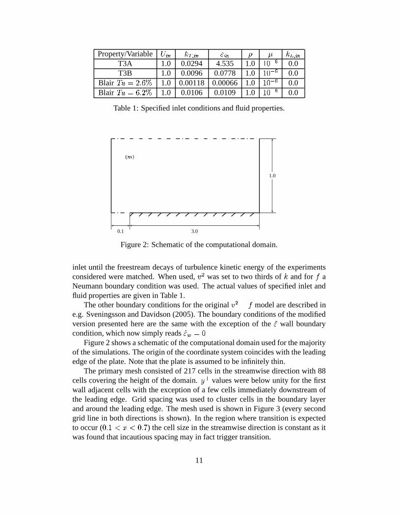
Table 1: Specified inlet conditions and fluid properties.

0.1 3.0

1.0

� ���

Figure 2: Schematic of the computational domain.

inlet until the freestream decays of turbulence kinetic energy of the experimentsconsidered were matched. When used, � � was set to two thirds of � and for � aNeumann boundary condition was used. The actual values of specified inlet andfluid properties are given in Table 1.

The other boundary conditions for the original � � � � model are described ine.g. Sveningsson and Davidson (2005). The boundary conditions of the modifiedversion presented here are the same with the exception of the � wall boundarycondition, which now simply reads ��� � �

Figure 2 shows a schematic of the computational domain used for the majorityof the simulations. The origin of the coordinate system coincides with the leadingedge of the plate. Note that the plate is assumed to be infinitely thin.

The primary mesh consisted of 217 cells in the streamwise direction with 88cells covering the height of the domain. ��� values were below unity for the firstwall adjacent cells with the exception of a few cells immediately downstream ofthe leading edge. Grid spacing was used to cluster cells in the boundary layerand around the leading edge. The mesh used is shown in Figure 3 (every secondgrid line in both directions is shown). In the region where transition is expectedto occur (

� � � �) the cell size in the streamwise direction is constant as it

was found that incautious spacing may in fact trigger transition.

11

Figure 3: Computational mesh. Every second grid line is shown.

To judge the level of convergence the momentum and continuity equationresiduals were scaled with momentum and mass flux through the inlet, respec-tively. Usually, when all scaled residuals reaches a level of

��� � or lower thecomputations can be considered as being fully converged but, as will be illustratedlater, these computations require extra care when judging convergence.

3.1 Comments on the test case used for validation

The main test cases considered for validation of the investigated models perfor-mance in transitional flows are the T3A and T3B cases used by the ERCOFTACSIG on Transition coordinated by Prof. Mark Savill, presently at the CranfieldUniversity. Both cases are considered zero pressure gradient flows over a flatplate and their only difference is the freestream turbulence intensity that in theT3A case is three percent and six percent in the T3B case. The experimental datawas obtained at the Rolls-Royce Applied Science Laboratory. A schematic of theexperimental rig is shown in Figure 4.

As can be seen from Figure 4 the plate in the experiment is not infinitelythin and has an apex shaped leading edge with a radius of 0.75 mm at the verybeginning of the plate. To avoid laminar separation at the leading edge the platein the experiment was inclined by about 0.5 degree.

A second set of data (Blair (1983)) was also used when validating the imple-mentation of the Walters and Leylek (2004) model for transitional flows. Thesedata are similar to the ERCOFTAC cases but the experimental set-up used allowedmuch larger turbulence length scales and can therefore be used as a complementto the ERCOFTAC data.

Important in CFD in general and in transition modelling in particular is toensure that computed results are independent of numerical aspects such as meshdensity and discretization, and that the boundary conditions are the same as inthe experiment used for validation. The numerics will be considered in the sec-tion to follow and we will here address the geometrical and boundary condition

12

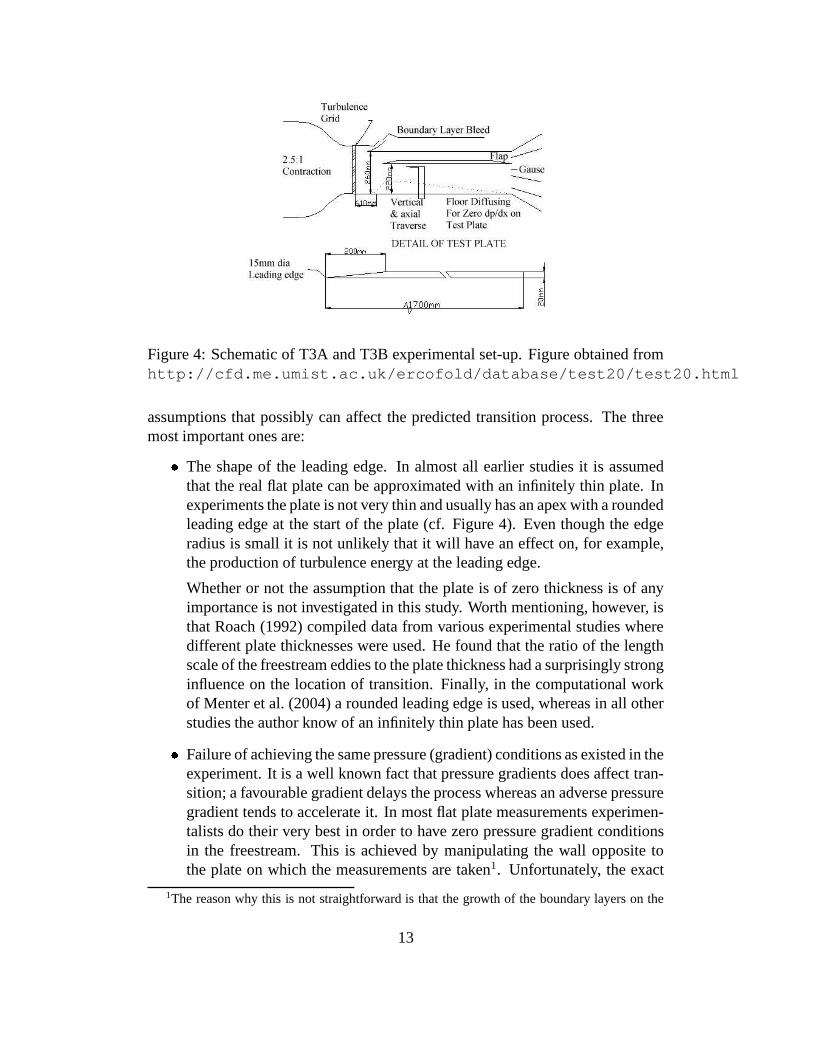
Figure 4: Schematic of T3A and T3B experimental set-up. Figure obtained fromhttp://cfd.me.umist.ac.uk/ercofold/database/test20/test20.html

assumptions that possibly can affect the predicted transition process. The threemost important ones are:

� The shape of the leading edge. In almost all earlier studies it is assumedthat the real flat plate can be approximated with an infinitely thin plate. Inexperiments the plate is not very thin and usually has an apex with a roundedleading edge at the start of the plate (cf. Figure 4). Even though the edgeradius is small it is not unlikely that it will have an effect on, for example,the production of turbulence energy at the leading edge.

Whether or not the assumption that the plate is of zero thickness is of anyimportance is not investigated in this study. Worth mentioning, however, isthat Roach (1992) compiled data from various experimental studies wheredifferent plate thicknesses were used. He found that the ratio of the lengthscale of the freestream eddies to the plate thickness had a surprisingly stronginfluence on the location of transition. Finally, in the computational workof Menter et al. (2004) a rounded leading edge is used, whereas in all otherstudies the author know of an infinitely thin plate has been used.

� Failure of achieving the same pressure (gradient) conditions as existed in theexperiment. It is a well known fact that pressure gradients does affect tran-sition; a favourable gradient delays the process whereas an adverse pressuregradient tends to accelerate it. In most flat plate measurements experimen-talists do their very best in order to have zero pressure gradient conditionsin the freestream. This is achieved by manipulating the wall opposite tothe plate on which the measurements are taken1. Unfortunately, the exact

1The reason why this is not straightforward is that the growth of the boundary layers on the

13

details of how these conditions are achieved are never given but instead theflow is categorized as a flat plate zero pressure gradient flow. Further, it isnot clear if the tilting of the flat plate itself affects the flow adjacent to it.The possible effects of these uncertainties can be investigated by increasingthe height of the domain or by tilting one of the two the walls.

� The position of the inlet relative to the leading edge of the plate. Many in-vestigations have showed that it is not adequate to have the inlet coincidingwith the leading edge of the plate. Therefore the plate is preceded by a shortregion (cf. Figure 2) where a symmetry boundary condition is applied. Thisway most uncertainties regarding what conditions to specify at the inlet areavoided as constant profiles can be specified for all quantities involved andthe flow will adjust as the flat plate is approached. However, it is not clearhow long an upstream distance is needed for the flow to adjust to the newconditions without being influenced by the choice of this distance. Notethat as soon as the flow senses the presence of the plate (via the pressureof elliptic nature) the flow will slow down/speed up, which may affect thepredicted turbulence production.

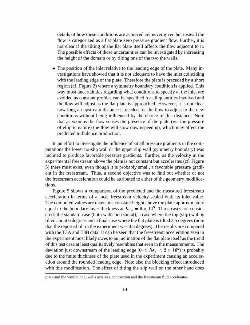
In an effort to investigate the influence of small pressure gradients in the com-putations the lower no-slip wall or the upper slip wall (symmetry boundary) wasinclined to produce favorable pressure gradients. Further, as the velocity in theexperimental freestream above the plate is not constant but accelerates (cf. Figure5) there must exist, even though it is probably small, a favorable pressure gradi-ent in the freestream. Thus, a second objective was to find out whether or notthe freestream acceleration could be attributed to either of the geometry modifica-tions.

Figure 5 shows a comparison of the predicted and the measured freestreamacceleration in terms of a local freestream velocity scaled with its inlet value.The computed values are taken at a constant height above the plate approximatelyequal to the boundary layer thickness at ����� � �� � � . Three cases are consid-ered: the standard case (both walls horizontal), a case where the top (slip) wall istilted about 6 degrees and a final case where the flat plate is tilted 2.5 degrees (notethat the reported tilt in the experiment was 0.5 degrees). The results are comparedwith the T3A and T3B data. It can be seen that the freestream acceleration seen inthe experiment most likely owes to an inclination of the flat plate itself as the trendof this test case at least qualitatively resembles that seen in the measurements. Thedeviation just downstream of the leading edge (

� ����� & � � � ) is probablydue to the finite thickness of the plate used in the experiment causing an acceler-ation around the rounded leading edge. Note also the blocking effect introducedwith this modification. The effect of tilting the slip wall on the other hand does

plate and the wind tunnel walls acts as a contraction and the freestream fluid accelerates.

14

−1 0 1 2 3 4 5 6

x 105

0.98

1

1.02

1.04

1.06

PSfrag replacements������

����

*

Inclined slip wallInclined plateHorizontal wallsT3A dataT3B data

Figure 5: Freestream acceleration owing to the effect of inclined walls.

not couple with freestream acceleration in the experiment which indicates that the(unknown) shape of the opposite wall is of minor importance as compared withthe tilting of the flat plate. Further, the result of the standard computation showsthat the freestream acceleration, and thus the favorable pressure gradient, is smalland therefore also that the extent of the domain normal to the plate is large enoughto have essentially zero pressure gradient conditions. Finally, the small variationin velocity upstream of the leading edge indicates that the computational inlet ispositioned sufficiently far upstream of the leading edge to prevent influence of theexact inlet position. Note however that this is not the case for the computationwith the inclined flat plate.

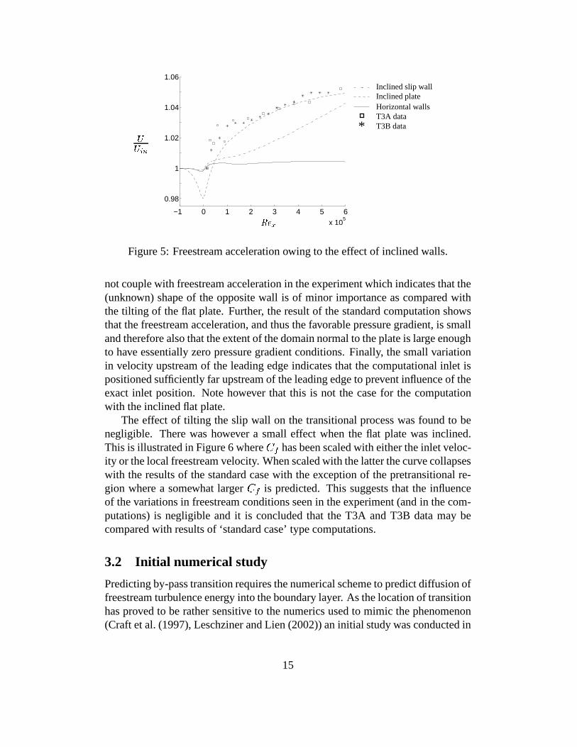
The effect of tilting the slip wall on the transitional process was found to benegligible. There was however a small effect when the flat plate was inclined.This is illustrated in Figure 6 where R has been scaled with either the inlet veloc-ity or the local freestream velocity. When scaled with the latter the curve collapseswith the results of the standard case with the exception of the pretransitional re-gion where a somewhat larger R is predicted. This suggests that the influenceof the variations in freestream conditions seen in the experiment (and in the com-putations) is negligible and it is concluded that the T3A and T3B data may becompared with results of ‘standard case’ type computations.

3.2 Initial numerical study

Predicting by-pass transition requires the numerical scheme to predict diffusion offreestream turbulence energy into the boundary layer. As the location of transitionhas proved to be rather sensitive to the numerics used to mimic the phenomenon(Craft et al. (1997), Leschziner and Lien (2002)) an initial study was conducted in

15

4 4.5 5 5.5 6−3

−2.8

−2.6

−2.4

−2.2

−2

PSfrag replacements���������

��� ��� �

� � ������ ������Standard case.

� � �T3A dataT3B data

Figure 6: The effect of wall inclination on skin friction coefficient, R . R is forthe tilted plate evaluated using two different scaling velocities.

order to find out how fine a grid is needed for the results to be grid independent.Also added are results of a computation on a domain of smaller physical size tosee if the location of the slip wall or the outlet has any influence on transition.

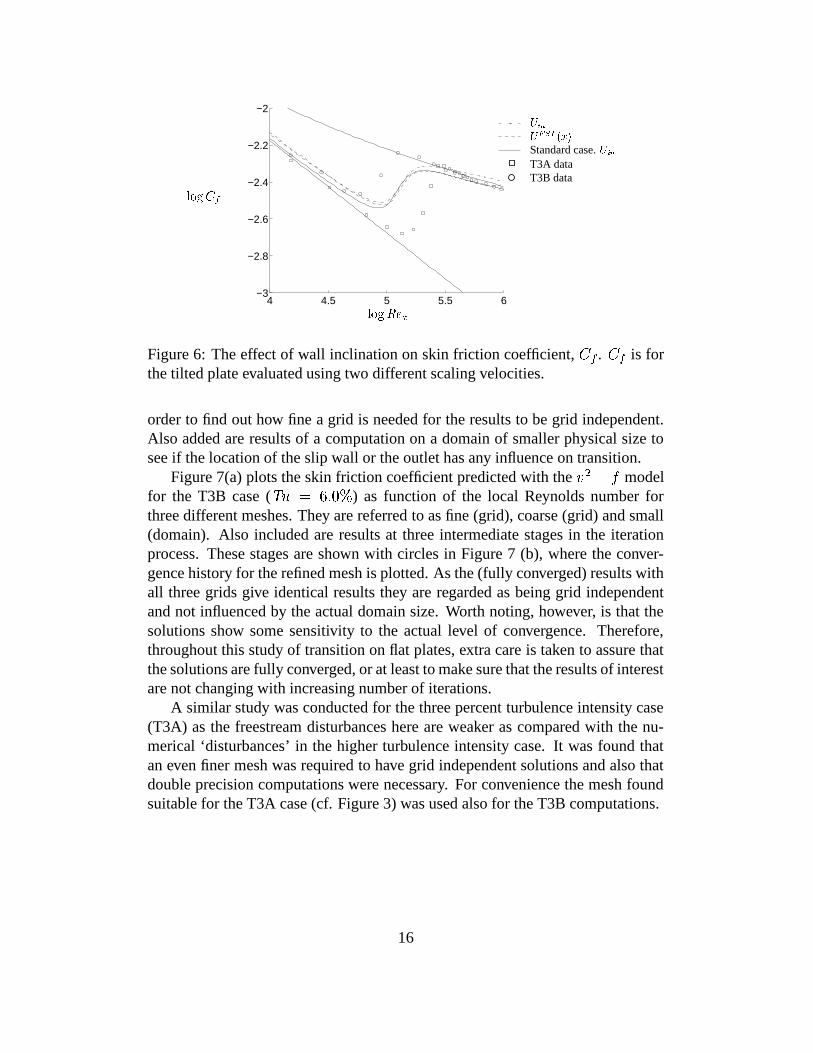
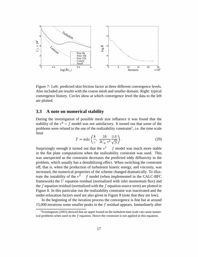
Figure 7(a) plots the skin friction coefficient predicted with the # * , . modelfor the T3B case ( ���

3 ]����! ) as function of the local Reynolds number forthree different meshes. They are referred to as fine (grid), coarse (grid) and small(domain). Also included are results at three intermediate stages in the iterationprocess. These stages are shown with circles in Figure 7 (b), where the conver-gence history for the refined mesh is plotted. As the (fully converged) results withall three grids give identical results they are regarded as being grid independentand not influenced by the actual domain size. Worth noting, however, is that thesolutions show some sensitivity to the actual level of convergence. Therefore,throughout this study of transition on flat plates, extra care is taken to assure thatthe solutions are fully converged, or at least to make sure that the results of interestare not changing with increasing number of iterations.

A similar study was conducted for the three percent turbulence intensity case(T3A) as the freestream disturbances here are weaker as compared with the nu-merical ‘disturbances’ in the higher turbulence intensity case. It was found thatan even finer mesh was required to have grid independent solutions and also thatdouble precision computations were necessary. For convenience the mesh foundsuitable for the T3A case (cf. Figure 3) was used also for the T3B computations.

16

4 4.5 5.5 60

2

4

6

8

PSfrag replacements

�������

��� ���������CoarseSmall

Fine 6kFine 10kFine 22k

0 5 10 15 20 25−5

−4

−3

−2

−1

PSfrag replacements

� ���

Iteration �������

Laminar

Turbulent

Figure 7: Left: predicted skin friction factor at three different convergence levels.Also included are results with the coarse mesh and smaller domain. Right: typicalconvergence history. Circles show at which convergence level the data to the leftare plotted.

3.3 A note on numerical stability

During the investigation of possible mesh size influence it was found that thestability of the � � � � model was not satisfactory. It turned out that some of theproblems were related to the use of the realizability constraint2, i.e. the time scalelimit 1 � � � � � �

& ��

�0/ ) � � �� ! � (29)

Surprisingly enough it turned out that the � � � � model was much more stablein the flat plate computations when the realizability constraint was used. Thiswas unexpected as the constraint decreases the predicted eddy diffusivity in theproblem, which usually has a destabilizing effect. When switching the constraintoff, that is, when the production of turbulence kinetic energy, and viscosity, wasincreased, the numerical properties of the scheme changed dramatically. To illus-trate the instability of the � � � � model (when implemented in the CALC-BFCframework) the

�equation residual (normalized with inlet momentum flux) and

the � equation residual (normalized with the � equation source term) are plotted inFigure 8. In this particular run the realizability constraint was inactivated and theunder-relaxation factors used are also given in Figure 8 (note that they are low).

In the beginning of the iteration process the convergence is fine but at around15,000 iterations some smaller peaks in the � residual appears. Immediately after

2Sveningsson (2003) showed that an upper bound on the turbulent time scale can cause numer-ical problems when used in the equation. Hence the constraint is not applied in this equation.

17

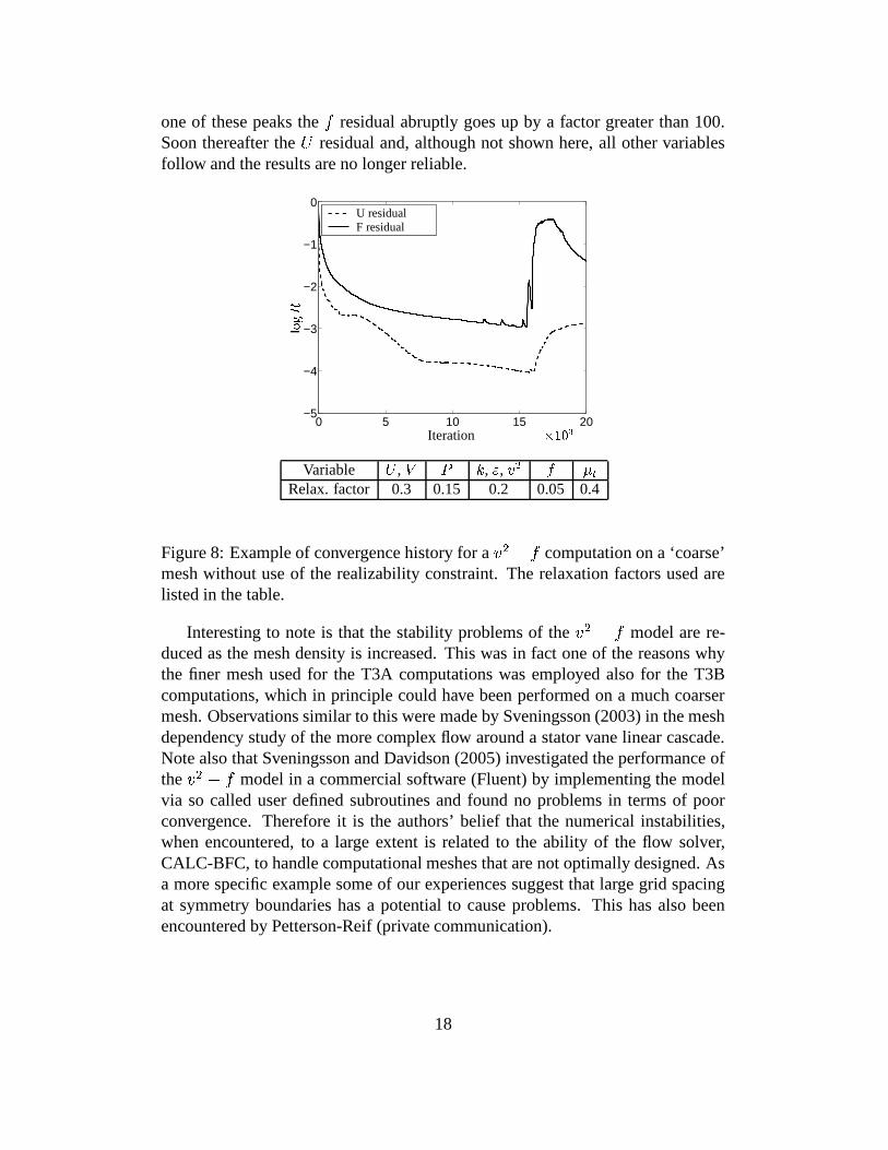
one of these peaks the � residual abruptly goes up by a factor greater than 100.Soon thereafter the

�residual and, although not shown here, all other variables

follow and the results are no longer reliable.

Variable � , � � � , � , ��� � �Relax. factor 0.3 0.15 0.2 0.05 0.4

0 5 10 15 20−5

−4

−3

−2

−1

0

PSfrag replacements� ���

Iteration ����� �

U residualF residual

Figure 8: Example of convergence history for a � � � � computation on a ‘coarse’mesh without use of the realizability constraint. The relaxation factors used arelisted in the table.

Interesting to note is that the stability problems of the ��� � � model are re-duced as the mesh density is increased. This was in fact one of the reasons whythe finer mesh used for the T3A computations was employed also for the T3Bcomputations, which in principle could have been performed on a much coarsermesh. Observations similar to this were made by Sveningsson (2003) in the meshdependency study of the more complex flow around a stator vane linear cascade.Note also that Sveningsson and Davidson (2005) investigated the performance ofthe � � � � model in a commercial software (Fluent) by implementing the modelvia so called user defined subroutines and found no problems in terms of poorconvergence. Therefore it is the authors’ belief that the numerical instabilities,when encountered, to a large extent is related to the ability of the flow solver,CALC-BFC, to handle computational meshes that are not optimally designed. Asa more specific example some of our experiences suggest that large grid spacingat symmetry boundaries has a potential to cause problems. This has also beenencountered by Petterson-Reif (private communication).

18

4 4.5 5 5.5 6−3

−2.8

−2.6

−2.4

−2.2

−2

PSfrag replacements

���������

��� ��� �

T3AT3BLam. solution & turb. corr.Exp. T3AExp. T3B

Figure 9: Response to elevated freestream turbulence of the #6* ,b. model.

4 Results

4.1 The Original � ����� Model

As a first illustration of the fact that RANS turbulence models indeed have a po-tential to predict the influence of freestream turbulence on a transitional boundarylayer the #�*-, . model (Cokljat et al., 2003) is considered. Figure 9 shows acomparison of the predicted skin friction coefficients of the T3A and T3B caseswith measured data. It can be seen that the model responds correctly to the in-crease in freestream turbulence as the point of transition onset moves upstreamfor the high turbulence intensity case. Another feature of the model is that thetransition to turbulence is not as abrupt as often seen with typical two-equationturbulence models, but is preceded with a gradual increase in R that qualitativelyresembles the trends seen in the experiment. The only problem, which indeed isthe motivation for the present study, is that transition onset occurs far too earlyfor both the high and low turbulence intensity cases. The results in Figure 9 werecomputed using a realizability constraint on the time scales appearing in the Lequation and the eddy-viscosity expression. The influence of the constraint in thisflow, however, is almost negligible.

4.2 The Model of Walters and Leylek (2004)

To validate the implementation of the original LKE model the model was tested ina 1D fully developed turbulent channel flow ( ���

3 e f ). The predicted profilesof �� , �X� , their sum and the predicted total dissipation rate (

NLU; 0 � ) are comparedwith the DNS of Kim et al. (1987) in Figure 10. It can be seen that the results agreewell with the DNS. Further, the results are identical to those given in Walters and

19

0 50 100 150 200 250 300 3500

1

2

3

4

5

6

PSfrag replacements

�����������

� �

��������� ��������DNS

�����DNS

�

Figure 10: Profiles of fluctuating energies and dissipation rate (

NL�; 0 � ) in a fullydeveloped turbulent channel flow. Results obtained with the model of Walters andLeylek (2004). Symbols show DNS data of Kim et al. (1987).

Leylek (2004). Thus it can be concluded that the fully turbulent behavior of thepresent implementation agrees with the original model.

To assess the implementation also in transitional flows the � �3 ] � c and

���3 c � ]! freestream turbulence case of Blair (1983) is considered. This is

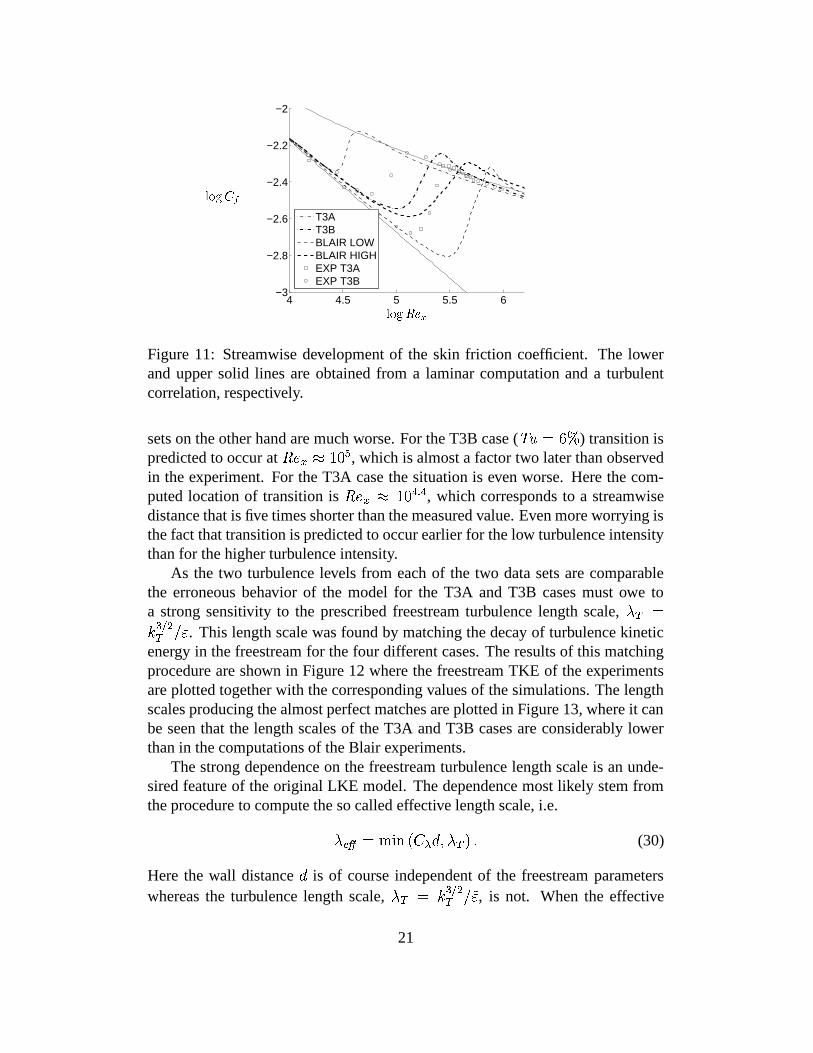
the same data as was used by Walters and Leylek (2004) to validate their model.A comparison with the results in Walters and Leylek (2004) shows perfect agree-ment in both transition length and location which suggests that the implementationworks well also in transitional flows. The predicted skin friction coefficients areshown in Figure 11 (dashed lines) but there is unfortunately no experimental skinfriction data to compare with.

The reason behind the efforts to convince the reader that the implementationof the model is free from errors is that in the early stages of this study only the ER-COFTAC test cases T3A (flat plate ���

3 e ���! ) and T3B (flat plate ���3 ]����! )

were considered. It turns out that the model of Walters and Leylek (2004) be-haves very differently for these conditions as compared with the test cases ofBlair (1983). This is illustrated in Figure 11 where the predicted skin frictioncoefficients are plotted for four different sets of freestream conditions (T3A, T3B,Blair 2.6% and Blair 6.2%). Also included are the experimental data for T3A(squares) and T3B (circles) together with the laminar solution (lower solid line)and a correlation for a fully turbulent boundary layer (upper solid line). Althoughnot shown here the agreement of the computations with the two data sets of Blair(1983) is good with the exception of a slight overshoot just downstream of thelocation where the transition is completed and the model responds as expected tothe increase in freestream turbulence level. The results for the ERCOFTAC data

20

4 4.5 5 5.5 6−3

−2.8

−2.6

−2.4

−2.2

−2

T3AT3BBLAIR LOWBLAIR HIGHEXP T3AEXP T3B

PSfrag replacements

��� ���

���� � � �

Figure 11: Streamwise development of the skin friction coefficient. The lowerand upper solid lines are obtained from a laminar computation and a turbulentcorrelation, respectively.

sets on the other hand are much worse. For the T3B case (�� � �

) transition ispredicted to occur at ��� � � � � , which is almost a factor two later than observedin the experiment. For the T3A case the situation is even worse. Here the com-puted location of transition is ����� � � � � � , which corresponds to a streamwisedistance that is five times shorter than the measured value. Even more worrying isthe fact that transition is predicted to occur earlier for the low turbulence intensitythan for the higher turbulence intensity.

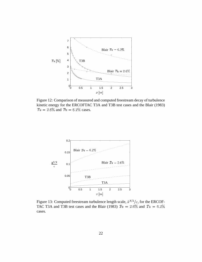
As the two turbulence levels from each of the two data sets are comparablethe erroneous behavior of the model for the T3A and T3B cases must owe toa strong sensitivity to the prescribed freestream turbulence length scale,

� � �

� �� �� � . This length scale was found by matching the decay of turbulence kineticenergy in the freestream for the four different cases. The results of this matchingprocedure are shown in Figure 12 where the freestream TKE of the experimentsare plotted together with the corresponding values of the simulations. The lengthscales producing the almost perfect matches are plotted in Figure 13, where it canbe seen that the length scales of the T3A and T3B cases are considerably lowerthan in the computations of the Blair experiments.

The strong dependence on the freestream turbulence length scale is an unde-sired feature of the original LKE model. The dependence most likely stem fromthe procedure to compute the so called effective length scale, i.e.� � � � � � � ��� � � � � (30)

Here the wall distance�

is of course independent of the freestream parameterswhereas the turbulence length scale,

� � � � �� �� ��� , is not. When the effective

21

0 0.5 1 1.5 2 2.5 30

1

2

3

4

5

6

7

PSfrag replacements

����� ���

� � �

Blair����� �� ���

Blair���������� ��

T3A

T3B

Figure 12: Comparison of measured and computed freestream decay of turbulencekinetic energy for the ERCOFTAC T3A and T3B test cases and the Blair (1983)���� & � � and

��� �� & � cases.

0 0.5 1 1.5 2 2.5 30

0.05

0.1

0.15

0.2

PSfrag replacements

��������

� � �

Blair������ �� ���

Blair���������� ��

T3A

T3B

Figure 13: Computed freestream turbulence length scale, � �� � � , for the ERCOF-TAC T3A and T3B test cases and the Blair (1983)

�� � & � � and�� � & �

cases.

22

0 1 2 3 4 50

0.005

0.01

0.015

0.02

PSfrag replacements

� � ��

�����

������ �

� ���

� ����� �

Figure 14: Profiles of the different length scales used to separate small scale en-ergy from large scale energy. Results from case T3B obtained with the model ofWalters and Leylek (2004) at ��� � � �� � �

.

length scale is used to split up the TKE into its small and large scale parts (cf. Eqn7) a decrease in � �� � � will lead to increasingly larger percentages small scaleTKE. Consequently, as the small scale energy contributes to the production ofTKE, this scenario has a potential to shorten the route to transition. In an effort toavoid having this problem also with the model suggested in the previous sectionthe wall distance based length scale was replaced according to��� � ����� � ��� � �(! � �� �� �

(31)

Figure 14 plots the turbulence length scale together with the two different lengthscales used to split the energy into small and large scale parts as function of walldistance in boundary layer height units. It can be seen that when the wall distancebased scale is used the intersection where the effective length scale switches to theturbulence length scale has no coupling to the extent of the boundary layer. Thus,a change in freestream length scale will have an effect on how far away from thewall the effective length scale will take its lower value. Under the circumstancesshown in Figure 14 the switch occurs at � � � �

and the larger the turbulencelength scale the further out switch takes place.

When using the length scale in Eqn 31 the switch always (at least in the flatplate case considered here) takes place at about the edge of the boundary layer.This construction is believed to reduce the sensitivity of the new model to theprescribed level of turbulence length scale in the freestream. Note, however, that areduced length scale extending well beyond the boundary layer affects turbulenceproduction also around stagnation points and will reduce the overproduction ofTKE that is usually avoided with a realizability constraint.

23

0 50 100 150 200 250 300 3500

1

2

3

4

5

6

PSfrag replacements

�����������

� �

����������DNS

�����DNS

�

Figure 15: Profiles of fluctuating energies and dissipation rate (

NL�; 0 � ) in a fullydeveloped turbulent channel flow. Results obtained with the modified #6* ,d.model. Symbols show DNS data of Kim et al. (1987).

4.3 The Modified � � � � Model

The extension and modifications to the original #&*�,K. model suggested in Sec-tion 2 where first validated against the DNS data of Kim et al. (1987) in the fullydeveloped turbulent channel flow. Figure 15 shows some results of this compari-son. Included are profiles of the predicted laminar and turbulence kinetic energy( �X� and �� ) and the (total) dissipation rate of �:� . The ��� profile is close to thatof the original # * , . model (not included here) and the predicted L profile fol-lows the DNS data closely. Note also the similarity of the L profile with that ofthe Walters and Leylek (2004) model (Figure 10). The main difference betweenthe modified and the Walters and Leylek (2004) models is that the former pre-dicts �X� 3

� throughout the channel whereas some LKE remains in the latter.This decoupling of the LKE from turbulent boundary layers was a desired featurethat allows modifications of the LKE equation without modifying the behavior inturbulent boundary layers.

Finally, the modified # * , . model was preliminary tested in a transitional flatplate flow. Figure 16 shows the development of the different components of thefluctuating energy together with a plot of the skin friction coefficient illustratingthe state of the boundary layer. It can be seen that after an initial growth of laminarkinetic energy (not shown here as it occurs upstream of the location in Figure 16b)it begins to transform into turbulent kinetic energy (Figure 16c). Shortly afterthis initial growth in �:� the production of ��� , EU� , is triggered and the transitionprocess accelerates. As ��� grows the function .�� ! (cf. Eqn 18-20) rapidly goesto zero, which consequently forces to production of �Y� to vanish as well. Withoutany additional production of ��� the I and

0 � sink terms soon bring �X� to zero,

24

which indeed is the desired scenario. Note that the new model captures the slightovershoot at the later stages of the transition but that the transitional process issomewhat to rapid (cf. Figure 16a).

The model was also tested in the T3A test case where it failed to reproducethe growth of the laminar kinetic energy. As the growth of � � was too smallthe production of ��� was not sufficiently dampened and transition was predictedto occur too early. This failure is likely due to the expression for the effectivelength scale and shows features similar to the failure of the Walters and Leylek(2004) model to predict the T3A and T3B cases. Thus, the expression for theeffective length scale suggested in Eqn 8 is probably not suitable for flows wherethe freestream turbulence length scale is small (i.e. the same problem as withthe Walters and Leylek (2004) model). In Figure 14 it can be seen that if thefreestream length scale is small (

��� � ���and smaller), the ratio of the effective

to turbulence length scale is relatively large and only a limited amount of theturbulence kinetic energy becomes large scale energy (cf. 7), which contributes toproduction of � � (cf. Eqn 10).

5 Concluding remarks

In this study the performance of two turbulence/transition models have been ex-amined. The first model, suggested by Walters and Leylek (2004), was found towork reasonably well in two transitional flat plate flows in which the freestreamturbulence length scale was relatively large. In two different test cases withsmaller length scales the model’s performance was considerably poorer, whichsuggests a strong length scale dependence of the model. The second model, de-veloped in this paper, adopts many of the transition specific features of the Waltersand Leylek (2004) model. The model is based on the � � � � model and the overallaim of this study has been to couple the � � � � model, which is known to performwell in turbulent flows, to the transition modelling approach of Walters and Leylek(2004) to improve the � ��� � model’s performance in transitional boundary layerflows.

Initial computations with the new model illustrated the potential of solving anadditional transport equation for a laminar fluctuating energy. The informationon the pretransitional boundary layer carried by this equation was used to modelthe by-pass transition mechanism suggested by e.g. Jacobs and Durbin (2001),i.e. that laminar streaks in the fluctuating u velocity component eventually breaksdown to form turbulent spots. Unfortunately, the new model inherited the sensi-tivity to the freestream length scale of the Walters and Leylek (2004) model and,thus, the measure to split the turbulent kinetic energy into small and large scalecomponents must be revised.

25

4.4 4.6 4.8 5 5.2 5.4 5.6

−2.6

−2.4

−2.2

−2

PSfrag replacements

0 0.5 1 1.5 20

0.002

0.004

0.006

0.008

0.01

PSfrag replacements

�����(a) ��� (b) ���� ��������������

0 0.5 1 1.5 20

0.002

0.004

0.006

0.008

0.01

PSfrag replacements

����� 0 0.5 1 1.5 20

0.002

0.004

0.006

0.008

0.01

PSfrag replacements

�����(c) ����� �� �!�"���$#�% (d) ���� ����������'&�&

0 0.5 1 1.5 20

0.005

0.01

0.015

0.02

PSfrag replacements

����� 0 0.5 1 1.5 20

0.005

0.01

0.015

0.02

PSfrag replacements

�����(e) ����� �� �!�"���$(*) (f) ���+ �� �!�,)-�/.�&

021436587

9 :�;�<>=�?

@A�BC'D

EGFEIHEGFKJLEIH

EGFEIHEGFKJLEMHE

T3B

Figure 16: Boundary layer profiles of the fluctuating energy components at posi-tions in the laminar, transitional and fully turbulent regions of the boundary layer.Circles show experimental data from the T3B test case.

26

References

Blair, M., 1983. Influence of free-stream turbulence on turbulent boundary layerheat transfer and mean profile development, part I–experimental data. Journalof Heat Transfer 105, 33–40.

Bradshaw, P., 1996. Turbulence modelling with application to turbomachinery.Proc. Aerospace Science 32, 575–624.

Brandt, L., Schlatter, P., Henningson, D. S., 2004. Transition in boundary layerssubject to free-stream turbulence. Journal of Fluid Mechanics 517, 167–198.

Byggstoyl, S., Kollmann, W., 1981. Closure model for intermittent turbulentflows. Int. J. of Heat and Mass Transfer 24, 1811–1821.

Cokljat, D., Kim, S., Iaccarino, G., Durbin, P., 2003. A comparative assessmentof the � � � � model for recirculating flows. AIAA-2003-0765.

Craft, T., Launder, B., Suga, K., 1997. Prediction of turbulent transitional phe-nomena with a nonlinear eddy-viscosity model. Int. J. Heat and Fluid Flow 18,15–28.

Davidson, L., Farhanieh, B., 1995. CALC-BFC: A finite-volume code employingcollocated variable arrangement and cartesian velocity components for compu-tation of fluid flow and heat transfer in complex three-dimensional geometries.Rept. 95/11, Dept. of Thermo and Fluid Dynamics, Chalmers University ofTechnology, Gothenburg.

Dopazo, C., 1977. On conditioned averages for intermittent turbulent flows. Jour-nal of Fluid Mechanics 81, 433–438.

Durbin, P., 1991. Near-wall turbulence closure modeling without ’damping func-tions’. Theoretical and Computational Fluid Dynamics 3, 1–13.

Jacobs, R., Durbin, P., 2001. Simulations of bypass transition. Journal of FluidMechanics 428, 185–212.

Kim, J., Moin, P., Moser, R., 1987. Turbulence statistics in fully developed chan-nel flow at low Reynolds number. Journal of Fluid Mechanics 177, 133–166.

Lardeau, S., Leschziner, M., Li, N., 2004. Modelling bypass transition with low-reynolds-number nonlinear eddy-viscosity closure. Flow, Turbulence and Com-bustion 73, 49–76.

27

Lardeau, S., Li, N., Leschziner, M., 2005. LES of transitional boundary layer athigh free-stream turbulence intensity, and implications for RANS modelling.In: 4th Int. Symp. on Turbulence and Shear Flow Phenomena. pp. 431–436.

Leschziner, M. A., Lien, F. S., 2002. Numerical aspects of applying second-moment closure to complex flows. In: Launder, B. E., Sandham, N. D. (Eds.),Closure Strategies for Turbulent and Transitional Flows. Cambridge UniversityPress, pp. 153–187.

Mayle, R., Schultz, A., 1997. The path to predicting bypass transition. Journal ofTurbomachinery 119, 405–411.

Menter, F., Langtry, R., Likki, S., Suzen, Y., Huang, P., Volker, S., 2004. A corre-lation based transition model using loacal variables part I – model formulation.In: ASME Turbo Expo 2004. Paper no. GT-2004-53452.

Pettersson-Reif, B. A., Durbin, P. A., Ooi, A., 1999. Modeling rotational effects ineddy-viscosity closures. International Journal of Heat and Fluid Flow, 563–573.

Radomsky, R., Thole, K., 2001. Detailed boundary layer measurements on a tur-bine stator vane at elevated freestream turbulence levels. Journal of Turboma-chinery 122, 666–676.

Roach, P. E., 1992. A correlation analysis approach to the T3 test case. In: Piron-neau, O., Rodi, W., Ryhming, I. L., Savill, A. M., Troung, T. V. (Eds.), Numer-ical Simualtion of Unsteady Flows and Transition to Turbulence. CambridgeUniversity Press, pp. 348–354.

Savill, A. M., 2002a. By-pass transition using conventional closures. In: Launder,B. E., Sandham, N. D. (Eds.), Closure Strategies for Turbulent and TransitionalFlows. Cambridge University Press, pp. 464–492.

Savill, A. M., 2002b. New strategies in modelling by-pass transition. In: Launder,B. E., Sandham, N. D. (Eds.), Closure Strategies for Turbulent and TransitionalFlows. Cambridge University Press, pp. 493–521.

Steelant, J., Dick, E., 1996. Modelling of bypass transition with conditionednavier-stokes equations coupled to an intermittency transport equation. Inter-national Journal of Numerical Methods in Fluids 23, 193–220.

Sveningsson, A., 2003. Analysis of the performacne of different � � � � turbulencemodels in a stator vane passage flow. Licentiate thesis, Dept. of Thermo andFluid Dynamics, Chalmers University of Technology, Gothenburg, Sweden.

28

Sveningsson, A., Davidson, L., 2005. Computations of flow field and heat transferin a stator vane passage using the � � - � turbulence model. Journal of Turboma-chinery 127, 627–634.

Walters, D., Leylek, J., 2004. A new model for boundary layer transition using asingle-point rans approach. Journal of Turbomachinery 126, 193–202.

Westin, K. J. A., Henkes, R. A. W. M., 1997. Application of turbulence models tobypass transition. Journal of Fluids Engineering 119, 859–866.

29