Towards an evolutionary cooperative gametheory

Andre Casajus and Harald Wiese, University of LeipzigPostfach 920, 04009 Leipzig, Germany,

tel.: 49 341 97 33 771,fax: 49 341 97 33 779

e-mail: wiese@wifa.uni-leipzig.de

February 2012

Abstract

The idea behind evolutionary game theory is to interpret payo¤s as�tness. Non-cooperative game theory has seen many interesting results andapplications. The aim of this paper is to introduce a replicator-dynamicsversion for cooperative game theory. We generate payo¤s, or �tness values,by way of the Mertens (1980) value which is a close cousin of the continuousShapley value introduced by Aumann & Shapley (1974). We already presentsome preliminary results for the resulting replicator dynamics (this part iswork in progress). We close with some (well-founded) conjectures on theevolutionary dynamics for particular TU games.Keywords: Mertens value, replicator dynamics, asymptotic stability,

apex gameJEL classi�cation: C71

1. Introduction

Evolutionary models of various forms have been part and parcel of economics fora long time (see, for example, the articles collected by Witt 1993). A speci�c classof models has been developed within game theory. In usual parlance, evolution-ary game theory (see, for example, Weibull (1995) or Samuelson (1997)) means

evolutionary theory applied to non-cooperative games. The aim of this paper isto develop an evolutionary cooperative game theory where we concentrate on thetransferable-utility case. Apparently, ideas in this direction have been around forsome time. Nasar (2002, p. xxiv) reports that John Nash, picking up his oldinterest in game theory, �received a grant from the National Science Foundationto develop a new �evolutionary�solution concept for cooperative games�.Cooperative game theory rests on two pillars. First, the economic (or political

or sociological ...) situation is described by a player set N and a coalition functionv : 2N ! ;. Subsets of N are called coalitions, with N being the grand coalition.For every coalitionK � N , v (K) is its worth that stands for the possibilities opento that coalition. For T 2 2Nn f;g ; the game uT is called the unanimity game; itis de�ned by uT (K) = 1 if T � K and uT (K) = 0 otherwise. The players from Tare often called the productive players while the other players are unproductive.As a second example, consider the apex game h for N = f1; :::; 4g : It is de�nedby

h (K) =

8<:1; 1 2 K and Kn f1g 6= ;1; K = Nn f1g0; otherwise

Thus, the apex player 1 needs one additional player to produce the worth 1: Thisworth can also be created by the coalition of the three less important players 2;3; and 4.Cooperative game theory�s second pillar are solution concepts, the most fa-

mous being the core and the Shapley�s (1953) value. From the point of view ofapplicability, the Shapley value has the advantage of producing unique payo¤s forthe n players. Thus, the coalition function is the input into a solution conceptand the payo¤ vector the output. For the above apex game, the Shapley payo¤vector is

Sh (N; v) =

�1

2;1

6;1

6;1

6

�:

Aumann &Myerson (1988) interpret the apex game as a weighted voting gameand try to predict coalition formation. They present a hybrid noncooperative-cooperative model which, following Brandenburger & Stuart (2007) (who use thecore rather than the Shapley value or the weighted XP Shapley value), can alsobe called a biform games. In that model, players (political parties) sequentiallydecide on forming links with other players. Depending on the links, the playersobtain the Myerson (1977) value which is an adaptation of the Shapley value fornetworks. Aumann & Myerson (1988) �nd that backward induction applied to

2

the link game leads to the coalition f2; 3; 4g where the three little players join toshare the worth of 1:In order to address problems of coalition formation (and for other purposes

as well), we take another approach by developping evolutionary cooperative gametheory. Imbedding games like the apex game into an evolutionary setting, weinterpret the payo¤s as �tness. A player�s success feeds into his proliferation. Inorder to model reproductive di¤erences between players, we distinguish betweenplayers (like the four players in the apex game) and agents who take up theroles (or types) of these n players. If a role is particularly fruitful (in producingrelatively high payo¤s for the agents assuming that role), the relative number ofthese agents increases.While the number of players is a natural number, we deal with a continuum

of agents for each player. Therefore, we need an extended coalition function thatis capable of dealing with non-integer players (agents). The Lovasz extension �vor the multi-linear (Owen) extension vMLE are suitable candidates. We prefer theLovasz extension to the multi-linear extension. If players (or agents) work together(in the framework of a unanimity or an apex game) and if the size of the agentsis below 1; the multilinear extension has a probabilistic interpretation (as notedby Owen 1972, p. 64) � the players work together only if their time scheduleshappen to coincide. For example, two productive players in the unanimity gameuf1;2g with s =

�12; 13

�can produce 1

2� 13, only. It seems to us that (by appropriate

coordination), the two agents should be able to produce the minimum of these two�gures, 1

3,. which is exactly what the Lovasz extension does. Also, consider s =

(2; 3). The multi-linear extension yields 2 � 3 = 6 whereas the minimum extensionleads to 2: Also, an extension�s worth may turn out to be negative even if theunderlying coalition function itself is positive. In fact, we �nd hMLE (2; 1; 3; 4) =�10: The use of the Lovasz extension has important repercussions for our model.In unanimity games, the productive players with minimal agent sets get all thepayo¤.Extensions of coalition functions cannot be an input for the (standard) Shapley

value. While the Lovasz extension �v is continuous, it is not di¤erentiable ingeneral. Hence, the diagonal formula introduced by Aumann & Shapley (1974)is not applicable. Fortunately, however, we can use the Mertens (1980) value asHaimanko (2001) has shown for a formally similar problem (of cost division). TheMertens value thus yields the payo¤ information understood as �tness and wecan then de�ne the replicator dynamics. Whenever an agent receives an above-average payo¤, the population share of his player will increase �a standard result

3

2

1

1, 44

33

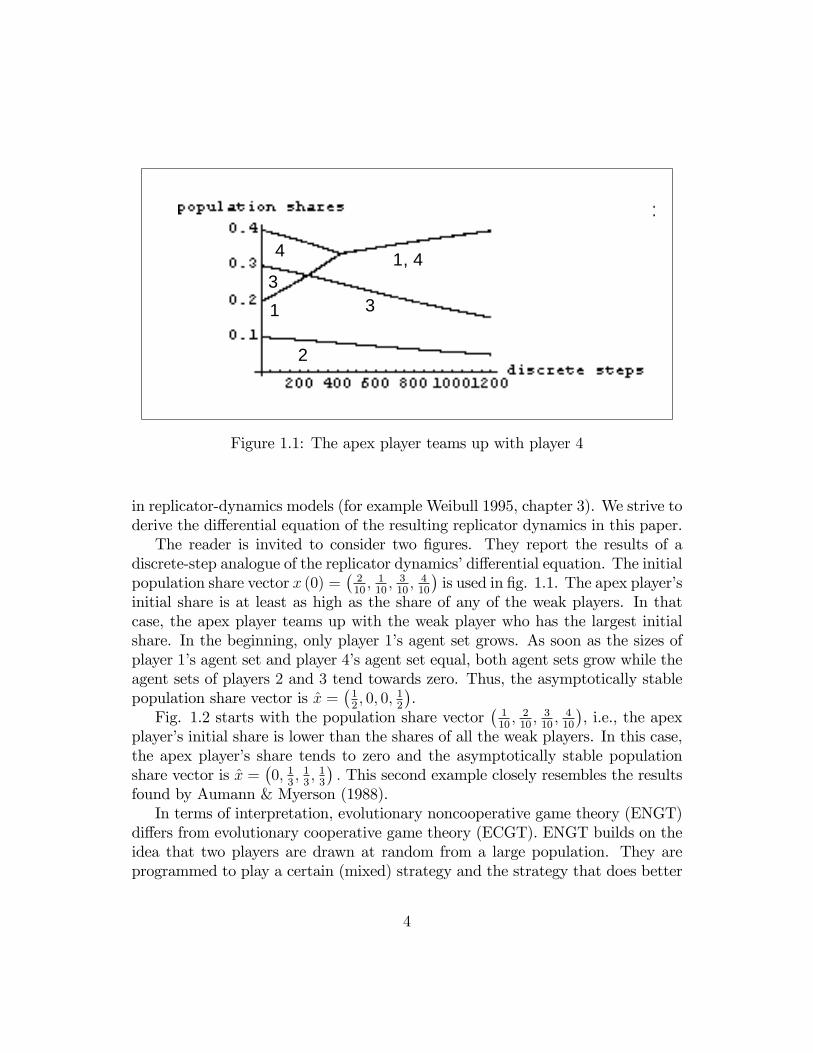
Figure 1.1: The apex player teams up with player 4

in replicator-dynamics models (for example Weibull 1995, chapter 3). We strive toderive the di¤erential equation of the resulting replicator dynamics in this paper.The reader is invited to consider two �gures. They report the results of a

discrete-step analogue of the replicator dynamics�di¤erential equation. The initialpopulation share vector x (0) =

�210; 110; 310; 410

�is used in �g. 1.1. The apex player�s

initial share is at least as high as the share of any of the weak players. In thatcase, the apex player teams up with the weak player who has the largest initialshare. In the beginning, only player 1�s agent set grows. As soon as the sizes ofplayer 1�s agent set and player 4�s agent set equal, both agent sets grow while theagent sets of players 2 and 3 tend towards zero. Thus, the asymptotically stablepopulation share vector is x̂ =

�12; 0; 0; 1

2

�.

Fig. 1.2 starts with the population share vector�110; 210; 310; 410

�, i.e., the apex

player�s initial share is lower than the shares of all the weak players. In this case,the apex player�s share tends to zero and the asymptotically stable populationshare vector is x̂ =

�0; 1

3; 13; 13

�: This second example closely resembles the results

found by Aumann & Myerson (1988).In terms of interpretation, evolutionary noncooperative game theory (ENGT)

di¤ers from evolutionary cooperative game theory (ECGT). ENGT builds on theidea that two players are drawn at random from a large population. They areprogrammed to play a certain (mixed) strategy and the strategy that does better

4

1

23 2, 3 2, 3, 4

4

Figure 1.2: The three unimportant players trump the apex player

than other strategies grows faster. The most basic model of ENGT builds on (a)�pairwise contests�and (b) a monomorphic population playing a symmetric game.Of course, more advanced ENGT models also deal with polymorphic playing-the-�eld situations.In contrast, the �simple�ECGT as presented here naturally belongs to (a) the

�playing the �eld�and (b) the polymorphic variety. (a) just results from the waythe Mertens value is calculated and interpreted �an agent�s payo¤ depends onthe set-up of the economy as a whole. (b) is the natural out�ow from di¤erentplayers�roles.We suggest to reserve the term ECGT for the non-atomic (or at least many-

agents) setup. It is the agents whose shares change. In contrast, one mightenvision a model where the players themselves grow or shrink. A suitable exampleis provided by �rms. Depending on their pro�ts they will grow in an organicfashion (rather than grow by mergers and acquisitions). This is not the kind ofmodel we have in mind in this paper.Our work is related to the concept of �dynamic cooperative games�introduced

by Filar & Petrosjan (2000). Their idea is to de�ne a sequence of games (in discreteor in continuous time) so that one TU game is determined by the previous oneand by the payo¤s achieved under some solution concept. The players (no agentsinvolved) in that paper obtain the sum of payo¤s for this sequence of coalitionfunctions. The authors deal with the problem of whether these payo¤s obey some

5

consistency criterion.When discussion the apex game, we argue that ECGT migth be considered a

contribution to the vast �eld of coalition formation. Alternatively, while a majorapplication of, and motivation for, ENGT is equilibrium selection (see the titel ofthe book by Samuelson 1997), ECGT focuses on the evolutionary pressure againstplayers (rather than strategy combinations). In particular, we derive the followingresults: 1. Dominated players (with lower marginal contributions) may survive inthe long run. 2. For simple games, asymptotically stable population share vectorsinvolve minimal winning coalitions.The paper is organized as follows. In the following section, we provide the

basics of TU games together with a de�nition of the Shapley value. Section3 introduces vector measure games for Lovasz extensions. We are then set toderive payo¤s by way of the Mertens value in section 4. We already presentsome preliminary results for the resulting replicator dynamics (this part is workin progress) in section 5. We then comment on some stability results in the section6 before concluding the paper with section 7.

2. Basic de�nitions and notation

2.1. Payo¤ vectors, population-size vectors

For a non-empty and �nite (player) set N , let

RN+ : =�x 2 RN j8i 2 N : xi � 0

;

RN++ : =�x 2 RN j8i 2 N : xi > 0

;

�N+ : =

�x 2 RN+ j

Pi2N xi = 1

;

�N++ : = �N

+ \ RN++:

2.2. Finite TU games

Let U be a su¢ ciently large in�nite set, the universe of players; N (U) denotes theset of non-empty and �nite set of subsets of U . A (TU) game on U is a pair(N; v) consisting of a set of players N 2 N (U) and a coalition function v 2V (N) :=

�f : 2N ! Rjf (;) = 0

. Subsets of N are called coalitions, and v (K)

is called the worth of coalition K.For v; w 2 V (N) ; � 2 R; the coalition functions v + w 2 V (N) and � � v 2

V (N) are given by (v + w) (K) = v (K)+w (K) and (� � v) (K) = � �v (K) for all

6

K � N: For K � N and v 2 V (N) ; vjK 2 V (K) denotes the restriction of v to2K : The null game on N is denoted (N;0) ; 0 2 V (N) ; where 0 (K) = 0 for allK � N: For T 2 2Nn f;g ; the game (N; uT ), uT (K) = 1 if T � K and uT (K) = 0otherwise, is called a unanimity game; the game (N; eT ), eT (K) = 1 if T = Kand eT (K) = 0 otherwise, is called a standard game. A game (N; v) is calledsimple i¤ v (K) 2 f0; 1g for all K � N ; it is called superadditive i¤ v (S [ T )� v (S) + v (T ) for all S; T � N; S \ T = ;: Let Vsa (N) and Vsi (N) denote thesets of superadditive and of simple coalition functions on N , respectively: Any v 2V (N) can be uniquely represented by unanimity games,

v =X

T�N :T 6=;

�T (v) � uT ; �T (v) :=X

S�T :S 6=;

(�1)jT j�jSj � v (S) : (2.1)

Player i 2 N is called a dummy player in (N; v) i¤ v (K [ fig) � v (K) =v (fig) for allK � Nn fig ; if in addition v (fig) = 0; then i is called a null player;players i; j 2 N are called symmetric in (N; v) if v (K [ fig) = v (K [ fjg) forall K � Nn fi; jg.A value on N is an operator ' that assigns a payo¤ vector ' (N; v) 2 RN

to any game (N; v) : An order of a set N is a bijection � : N ! f1; : : : ; jN jgwith the interpretation that i is the � (i)th player in �. The set of these ordersis denoted by R (N) : The set of players weakly preceding i in � is denoted byKi (�) = fj 2 N : � (j) � � (i)g : For i =2 K, the marginal contribution of i atK is de�ned by MCvi (K) := v (K[fig) � v (K) : The marginal contributionof i under � is denoted MCvi (�) := MC

vi (Ki (�) n fig) : The Shapley value on

V (N), Sh, is given by

Shi (N; v) :=1

jR (N)jX

�2R(N)

MCvi (�) ; i 2 N; v 2 V (N) : (2.2)

3. Vector measure games

3.1. De�nition

Let I be a set and C a subset of 2I such that (I; C) is isomorphic to ([0; 1] ;B) ;where B stands for the Borel subsets of [0; 1] : A game on (I; C) is a mappingv : C ! R such that v (;) = 0: A game is �nitely additive if v (S [ T ) =v (S) [ v (T ) for all S; T 2 C; S \ T = ;: A value ' on (I; C) is linear operatorthat assigns to any game v a �nitely additive game 'v and that is symmetric,positive, and e¢ cient (see Neyman 2002, Section 3).

7

( )vN,

game coalition solution conc.

( )vN,

( )( )vNvNi

si

s ,,~ ∈= µ

TU game

Lovasz extension

derived vectormeasure game

NK 2∈

NRs +∈

Shapley value

Mertens valueC∈C

vector measure game C∈C Diagonal formula:a) Aumann/Shapleyb) Mertens

Figure 3.1: From a TU game to a vector measure game

A game v on (I; C) is called a vector measure game if there is a triple�N; (�i)i2N ; f

�;

where N is a non-empty and �nite set N; �i; i 2 N is non-atomic on (I; C) ; andf is a function f : RN+ ! R such that

v := f � �;

where � is the vector measure � : C ! RN+ given by

� (C) = (�i (C))i2N ; C 2 C:

Abusing notation, we the write v =�N; (�i)i2N ; f

�:

Consider �g. 3.1. So far, we have presented TU games and vector measuregames in general. The next two subsections are devoted to the Lovasz extensionand the derived vector measure game while section 4 deals with the solutionconcepts.

8

3.2. The Lovasz extension

The Lovasz (1983) extension (N; �v) ; �v : RN+ ! R of a TU game (N; �v) is given by

�v (s) :=X

T�N;T 6=;

�T (v) �minT (s) ; s 2 RN+ ; (3.1)

where

minK : RN ! R; s 7! minK (s) := mini2K

si; K � N;K 6= ;: (3.2)

For unanimity games this implies

�uT (s) = minT (s) ; T � N; T 6= ;; s 2 RN+ : (3.3)

By (3.1) and (3.2), the Lovasz extension is linear in the coalition function,�v + �w = � � �v + � � �w for all v; w 2 V (N) ; and �; � 2 R; and non-negativelyhomogenous in s, �v (� � s) = ���v (s) for all v and � 2 R+ (see Lovasz 1983, Algaba,Bilbao, Fernandez & Jimenez 2004).Note that while themin-operator is continuous, it is not partially di¤erentiable.

Of course, this peculiarity is passed on to �v:

3.3. Derived vector measure game

From (N; v) ; v 2 V (N) and s 2 RN+ ; we construct a vector measure game ~vs =�N; (�si )i2N ; �v

�on (I; C) (isomorphic to ([0; 1] ;B)) as follows: There is a collection

(Ai)i2N , Ai 2 C with the following properties:D1 �si ; i 2 N is a measure on (I; C) :D2 For all i; j 2 N; i 6= j; we have Ai \ Aj = ;:D3 �si (C) = �

si (Ai \ C) ; i 2 N , C 2 C:

D4 �si (Ai) = si; i 2 N .

Remark 1. The intendend interpretation is the following: The set I containsthe agents of the players in N: Since we do not require the collection (Ai)i2N tobe exhaustive, I may contain additional agents, which are, however, completelyunproductive. The set C contains all coalitions under consideration. For all i 2N; the coalition Ai contains all agents of player i and no agents of the playersj 2 Nn fig : The measure �si ; i 2 N assigns to any coalition C 2 C the number of

9

agents of player i contained in it: Overall, there are �si (I) = �si (Ai) = si agentsof player i which only inhabit Ai: The vector measure � assigns to any C 2 Cthe vector �s (C) of �population sizes�of the players from N in C: Finally, theLovasz extension �v determines the worth generated by any C 2 C based on these�population sizes�.

Remark 2. It is easy to see that such a vector measure game ~vs =�N; (�si )i2N ; �v

�on some (I; C) always exists. Let (I; C) = ([0; 1] ;B) : Consider a injection � : N !f1; : : : jN jg and let Ai :=

��(i)�1jN j ;

�(i)jN j

�and �si be given by the density function

�si : [0; 1]! R;

�si (x) :=

�jN j � si; x 2 Ai;0; x 2 InAi;

x 2 [0; 1] ; i 2 N;

and the Lebesgue measure on [0; 1].

Remark 3. Given (N; v) and s 2 RN+ ; there is a lot of arbitrariness in choosing(I; C) and (Ai; �si )i2N as above. Ultimately, we are interested in the payo¤s of thecoalitions Ai; i 2 N only. Under the value applied, as we will see later on, thesepayo¤s are not sensitive to the unspeci�ed details.

4. Payo¤s for the vector measure game

Now, we determine the payo¤s ' (Ai) ; i 2 N for the vector measure games ~vs =�N; (�si )i2N ; �v

�; s 2 RN+ ; on (I; C) :

Note that for vector measure games v =�N; (�i)i2N ; f

�on (I; C), where f

is continuously di¤erentiable and �i (I) > 0; i 2 N , there is a convenient wayto determine the value, the diagonal formula by Aumann & Shapley (1974,Theorem B), also see Neyman (2002, pp. 2141). Alas, since the Lovasz extension�v is not di¤erentiable in general, we build on this approach.Fortunately, however, the games ~vs; s 2 RN+ belong to a class of games on

(I; C) on which the Mertens value (Mertens 1980) is the unique value (Neyman,2002, Section 8; Haimanko, 2001). In particular, Haimanko deals with vectormeasure games v =

�N; (�i)i2N ; f

�; with following properties:

H1 �i; i 2 N is a probability measure.

H2 The probability measures �i; i 2 N are mutually singular, i.e., they havepairwise di¤erent carriers.

10

H3 The function f is continuous and piecewise linear.It is easy to see that ~vs =

�N; (�si )i2N ; �v

�can be written to match this speci-

�cation, i.e.,~vs =

�N; (�si )i2N ; �v

�=�N; (�̂si )i2N ; �v

s�: (4.1)

For i 2 N; si > 0; the probability measure �i is given by

�̂si (C) =�si (C)

si; (4.2)

for i 2 N; si = 0; choose any probability measure �̂si such that �̂si (Ai) = 1 and�̂si (C) = �̂

si (Ai \ C) ; i 2 N , C 2 C. Further, let

hs : RN+ ! RN+ ; (xi)i2N 7! hs (x) = (si � xi)i2N ; x 2 RN+ (4.3)

and set�vs = �v � hs: (4.4)

By (4.2), D1, and D4,�N; (�i)i2N ; �v

s�meets H1. By (4.2), D1, and D4,�

N; (�i)i2N ; �vs�obeys H2. To see, H3, set

RN+ (�) : = RN+ \ RN (�) ; (4.5)

RN (�) : =�x 2 RN j8i; j 2 N : � (i) < � (j) () xi > xj

; � 2 R (N) :

By (3.1), (3.2), and (4.5), �v is continuous on RN+ and linear on the closure ofRN+ (�) ; � 2 R (N) : By (4.3) and (4.4), these properties are pased on from �v to�vs:

RN++ (�) : = RN++ \ RN+ (�)�N+ (�) : = �N+ \ RN+ (�)�N++ (�) : = �N+ \ RN++ (�)RN+ (R) : =

[�2R(N)

RN+ (�)

s 2 RN+ (R)

11

The Mertens value 'M on the class of vector measure games�N; (�i)i2N ; f

�obeying H1�H3 is given by the following diagonal formula (Neyman 2002, pp.2150)1:

'M (f � �) (C) = EYZ 1

0

@f (t � 1N ;Y ;� (C)) dt; C 2 C; (4.6)

where 1N 2 RN ; (1N)i = 1; i 2 N; Y = (Yi)i2N is a vector of independent randomvaribles, each with the standard Cauchy distribution and

@f (x; y; z) := lim"#0

fy+"z (x)� fy (x)" � kzk ; x 2 (0; 1)N ; y; z 2 RN ; (4.7)

where fy (x) ; x 2 (0; 1)N ; y 2 RN is the directional derivative of f at x in thedirection of y: Note that for each �xed x, @f (x; y; z) is the directional derivativeof the function y 7! fy (x) at y in the direction of z 2 RN :2Recall that the density d of a random variable Y on R with the standard

Cauchy distribution is

d (y) =1

� (1 + y2); x 2 R.

Hence, the density d of a vector Y = (Yi)i2N of independent random variables,each with standard Cauchy distribution, on RN is

d (y) =Yi2N

1

� (1 + y2i ); y 2 RN : (4.8)

Since both the Lovasz extention and Mertens value are linear in the coalitionfunction, respectively, we have

'M (�v � �s) (Ai) = 'M (�vs � �̂s) (Ai)

=X

T�N;T 6=;

�T (v) � 'M (�usT � �̂s) (Ai) (4.9)

for all i 2 N and v 2 V (N) :1Note that there is a misprint on Neyman (2002, p. 2150)� the obvoius expectation operator

EY is missing.2Since z is not normalized to kzk = 1; the nominator of the above formula should be " � kzk

and not just z as on Neyman (2002, p. 2150).

12

Fix i 2 N and T � N; T 6= ;: In order to determine 'M (�usT � �̂s) (Ai) ; we �rstcalculate the expression

@�usT (t � 1N ; y; �̂s (Ai)) ; t 2 [0; 1] ; y 2 RNn f0Ng :

By D4 and (4.2), we have �̂s (Ai) = 1i 2 RN ; (1i)i = 1, (1i)j = 0 for j 2 Nn fjg :Further by (4.7),

@�usT (t1N ; y; �̂s (Ai))

= lim"#0

(�usT )y+"�1i (t � 1N)� (�usT )y (t � 1N)

" � k1ik

= lim"#0

lim�#0

��usT (t � 1N + � � (y + " � 1i))� �usT (t � 1N)

� � ky + " � 1ik� : : :

"

: : :�usT (t � 1N + � � y)� �usT (t � 1N)

� � kyk

�; (4.10)

where k�k denotes the Euklidean norm operator.For K � N; K 6= ;; set argminK (x) := fj 2 Kjxj = minK (x)g ; x 2 RN . We

distinguish some cases.Case (i): We consider i 2 Nn argminT (s) : By (3.2), (3.3), and (4.4), we have

�usT (t � 1N) = t �minT (s) : (4.11)

Further, for su¢ ciently small " and �;

�usT (t � 1N + � � (y + " � 1i)) = �usT (t � 1N + � � y) = minT (s)��t+ � �minargminT (s) (y)

�:

Hence, (4.10) becomes

@�usT (t1N ; y; �̂s (Ai)) = minT (s) �minargminT (s) (y) � lim"#0

�1

ky + " � 1ik� 1

kyk

�"

= � yi

kyk kyk2�minT (s) �minargminT (s) (y) : (4.12)

For y 2 RN ; let y(�i) 2 RN be given by y(�i)i = �yi and y(�i)j = �yj forj 2 Nn fig : By (4.12), we have

@�usT�t1N ; y

(�i); �̂s (Ai)�= �@�usT (t1N ; y; �̂s (Ai)) : (4.13)

13

By (4.8), d�y(�i)

�= d (y) ; y 2 RN : Hence, (4.13), (4.6), and (4.1) already

entail'M (�uT � �s) (Ai) = 0: (4.14)

Case (ii): i 2 argminT (s) : Since Y is non-atomic, we are allowed to restrictattention to

y 2 RN (R) =[

�2R(N)

RN (�) :

Case (iia): i 6= argminargminT (s) (y) :The arguments of Case (i) apply up to (4.12), i.e.,

@�usT (t1N ; y; �̂s (Ai)) = �

yi

kyk kyk2�minT (s) �minargminT (s) (y) (4.15)

Case (iib): i = argminargminT (s) (y) : For su¢ ciently small " and �;

�usT (t � 1N + � � (y + " � 1i)) = minT (s) ��t+ � �

�minargminT (s) (y) + "

���usT (t � 1N + � � y) = minT (s) �

�t+ � �minargminT (s) (y)

�:

Hence together with (4.11), (4.10) becomes

@�usT (t1N ; y; �̂s (Ai)) = minT (s) � lim

"#0

yi + "

ky + " � 1ik� yikyk

"

= minT (s) �1

kykkyk2 � y2ikyk2

: (4.16)

For y 2 RN ; i; j 2 argminT (s) ; i 6= j; let y(i$j) 2 RN be given by y(i$j)i = yj;

y(i$j)j = yi and y

(i$j)j = �j for j 2 Nn fi; jg : By (4.15) and (4.16), we have

@�usT�t1N ; y

(i$j); �̂s (Ai)�= @�usT (t1N ; y; �̂

s (Aj)) : (4.17)

Further by (4.8), d�y(i$j)

�= d (y) ; y 2 RN : Hence, (4.17), (4.6), and (4.1) already

entail'M (�uT � �s) (Ai) = 'M (�v � �s) (Aj) : (4.18)

Now, consider �A := In[

i2NAi: By D3 and (4.2), �̂s

��A�= 0N 2 RN : Hence

by (4.6), (4.7), and (4.1),

'M (�uT � �s)��A�= 0: (4.19)

14

By (3.3), D3, and D4, the e¢ cency of the Mertens value entails

�uT � �s (I) = minT (s) :

Hence, (4.14), (4.18), and (4.19) entail

'M (�uT � �s) (Ai) =(0; i 2 Nn argminT (s) ;

sijargminT (s)j

; i 2 argminT (s) ; i 2 N: (4.20)

Further, (4.9) gives

'M (�v � �s) (Ai) = si �X

T�N :i2argminT (s)

�T (v)

jargminT (s)j: (4.21)

For i 2 N; s 2 RN+ (�) ; � 2 R (N) ; by (4.5) and (4.9), (4.21)

'M (�v � �s) (Ai) =X

T�Ki(�);i2T

minT (s)��T (v) = si�X

T�Ki(�);i2T

�T (v) = si�MCvi (�) :

(4.22)The importance of the afore mentioned formula lies in the fact that all whatmatters in the following are the payo¤s for

s 2 RN+ (R) :=[

�2R(N)

RN+ (�) :

For the sake of completeness, we povide the a formula for general s 2 RN+ : Wehave

'M (�v � �s) (Ai) =1

jR (N; s)jX

�2R(N;s)

si �MCvi (�) ; i 2 N; s 2 RN+ ; (4.23)

where

R (N; s) = f� 2 R (N) j8i; j 2 N : � (i) > � (j) () si < sjg ; s 2 RN+ :(4.24)

First note that (4.21) is special case of (4.23) because R (N; s) = � for s 2 RN+ (�).Since 'M is linear in v, it su¢ ces to show (4.23) for uT ; T � N; N 6= ;: For� 2 R (N; uT ) ; the marginal contributions MCuTi (�) are either 0 or 1: By (4.24),the marginal contribution MCuTi (�) is 1 i¤ i is the last player from argminT (s) :

15

Since by (4.24) the probability being the last one from argminT (s) in � is thesame for all i 2 argminT (s) ; we have

1

jR (N; s)jX

�2R(N;s)

si �MCvi (�) =si

jargminT (s)j= 'M (�uT � �s) (Ai) ;

which proves the claim.

5. Replicator dynamics derived from TU games

5.1. Basic idea

The basic idea of this section is to interpret the payo¤s

f vi (s) := 'M (�v � �s) (Ai) = si �X

T�N :i2argminT (s)

�T (v)

jargminT (s)j; (5.1)

i 2 N; v 2 V (N) ; s 2 RN+ as �tness of the populations of the players�agentswhich determine the velocities of their growth in time. Let

f v : RN+ ! RN ; s 7! (f vi (s))i2N ; s 2 RN+ :

For some �xed v 2 V (N) ; we obtain the following replicator dynamics for theabsolut population sizes given by the ordinary di¤erential equation

_s =ds

dt= f v (s) ; s 2 RN+ : (5.2)

For population shares, we obtain

_x =dx

dt= 'v (x) ; x 2 �N

+ ; (5.3)

where 'v : �N+ ! RN ; x 7! ('vi (x))i2N is given by

'vi (x) := fvi (x)� xi

Xj2N

f vj (x) ; i 2 N; x 2 �N+ : (5.4)

One easily checks that (5.3) is a replicator dynamic.

16

5.2. Solutions to the di¤erential equations

By (5.1) and (5.4), the right-hand sides of the ODE (5.2) and (5.3) are discountin-uous in general. Hence, the standard results on ODE (see e.g. Weibull 1995, Sec-tion 6) do not apply. Instead, we employ the Filippov (1988) approach later on(see Section 5.3)While the ODE (5.2) and (5.3) are discountinuous in general, it is immedi-

ate, again from (5.1) and (5.4), that they are Lipschitz continuous on certainsubdomains of RN+ or �N

+ ; respectively, on RN+ (�) and

�N+ (�) := �

N+ \ RN (�) ; � 2 R (N) :

Hence, Weibull (1995, Theorem 6.1) guarantees the existence of unique (local)solutions Weibull (1995, De�nition 6.1) of the ODE (5.2) and (5.3) on

RN++ (�) := RN++ \ RN (�) and �N++ (�) := �

N++ \ RN (�)

through any point s0 2 RN++ (�) and x0 2 �N++ (�) ; respectively. These solutions

are either global or reach the boundary of the domain in �nite time.In particular, the right-hand side of the ODE (5.2) is not only linear, but has

a rather simple structure. By (4.22), it is just the inner product of the populationsize vector with the vector of marginal contributions. One easily checks that theunique local solution of the ODE (5.2) on RN++ (�) through s0 2 RN++ (�) at t = 0is given by

si�t; s0

�= s0i � et�MCvi (�); i 2 N; t 2 T; (5.5)

where T � R is an open interval containing 0: Hence, the unique local solution ofthe ODE (5.3) on �N

++ (�) through x0 2 �N

++ (�) at t = 0 is given by

xi�t; x0

�=

x0i � et�MCvi (�)Pj2N x

0j � et�MCvj (�)

; i 2 N; t 2 T: (5.6)

Using (5.5 or (5.6), one can dertermine which domain of (potential) dicon-tinuity is reached when one starts at s0 2 RN++ (�) or x0 2 �N

++ (�). An or-dered partition (P ; �) on N is a partition P 2 P (N) together with a bijection� : P ! f1; : : : ; jPjg : Let Po (N) denote the set of all ordered partitions of N:

17

For (P ; �) 2 Po (N) ; setRN (P ; �) :=

�x 2 RN j8i; j 2 N : xi � xj () � (P (i)) � � (P (j))

;

RN+ (P ; �) := RN (P ; �) \ RN+ ;RN++ (P ; �) : = RN (P ; �) \ RN++;�N+ (P ; �) = RN (P ; �) \�N

+ ;

�N++ (P ; �) = RN (P ; �) \�N

++:

For i; j 2 N; i 6= j; s0 2 RN++; v 2 V (N) ; and � 2 R (N) ; set

t�i; j; v; s0; �

�=

8>><>>:+1; MCvi (�) =MC

vj (�)

_��MCvi (�)�MCvj (�)

� �s0i � s0j

�> 0

�;

��ln s0i � ln s0j

�MCvi (�)�MCvj (�)

;�MCvi (�)�MCvj (�)

� �s0i � s0j

�< 0:

Further, for s0 2 RN++; v 2 V (N) ; and � 2 R (N) ; lett��v; s0; �

�= min

i;j2N :i6=jt�i; j; v; s0; �

�:

By (5.5 or (5.6), t� (v; s0; �) is the time when the forward solution reaches theboundary of RN++ (�) or �N

++ (�) ; respectively. Note that if t� (v; s0; �) = +1;

then the trajectory stays in �N++ (�) for t � 0:

For s0 2 RN++; v 2 V (N) ; and � 2 R (N), set P (v; s0; �) 2 P (N) :P�v; s0; �

�(i) = fig[

�j 2 Nn fig jt

�i; j; v; s0; �

�= t�

�v; s0; �

�6= +1

; i 2 N;

and let � (v; s0; �) be the bijection P (v; s0; �)! f1; : : : ; jP (v; s0; �)jg given by��v; s0; �

� �P�v; s0; �

�(i)�

� ��v; s0; �

� �P�v; s0; �

�(j)�

() si�t��v; s0; �

�; s0�� sj

�t��v; s0; �

�; s0�;

i; j 2 N:

s0i � et�MCvi (�) = s0j � et�MCvj (�)

s0is0j� et�(MCvi (�)�MCvj (�)) = 1�

ln s0i � ln s0j�+ t �

�MCvi (�)�MCvj (�)

�= 0

t =��ln s0i � ln s0j

�MCvi (�)�MCvj (�)

=

18

5.3. Solutions to di¤erential equations with discontinuous right-handsides: General approach

Filippov (1988, Paragraph 4) considers the following setup.3

1. Let G � Rn; n 2 N.

2. Let f : G! Rn be piecewise continuous, i.e., G consist of

1. a �nite number ` 2 N of domains Gi � G; i = 1; : : : ; `;2. and a set M � G of measure zero, which consists of the boundarypoints of the Gi; i = 1; : : : ; `; and

3. f is continuous on the inner of any Gi � G; i = 1; : : : ; `;

4. for i = 1; : : : ; `; f on Gi can be extended continuously to the boundary ofGi; i.e., for any sequence (xk)k2N in Gi such that xk ! x 2M; the sequence(f (xk))k2N coverges to some x 2 Rn:

5. M consists of a �nite number of hyperplanes.

From the point-valued vector �eld f : G ! Rn; one obtains the set-valuedvector �eld F : G� Rn;

F (x) =

�ff (x)g ; x 2 GnM;con flimxk2Gi:xk!x f (xk) ji = 1; : : : ; `; x 2 @Gig x 2M;

where con (A) and @ (A) denote the convex hull and the boundary of A � Rnrespectively.A solution to the ODE _x = f (x) is a solution of the di¤erential inclusion

_x 2 F (x) ; i.e., an absolutely continuous function x : I ! Rn on some intervalI � R containing 0 for which _x (t) 2 F (x) almost everywhere on I:Filippov (1988, pp. 81) presents the following results on the solutions to ODE

as above:

A. Through any point of the interior of G there passes a solution.

B. Each solution lying within a given closed bounded domain is continued onboth sides to reach the boundary of the domain.

3Actually, we restrict attention to autonomous ODE with discontinuous right-hand sides.Further, we focus on hypersurfaces that are hyperplanes.

19

5.4. Solutions to di¤erential equations with discontinuous right-handsides: Population dynamic

Fortunately, the ODE (5.2) and (5.3) �t the setup outlined in Section 5.3. Thedomains of continuity are

�RN+ (�)

��2R(N) and

��N+ (�)

��2R(N) ; respectively; the

domains of (potential) discontinuity are�RN+ (P ; �)

�(P;�)2Po (N) and

��N+ (P ; �)

�(P;�)2Po (N) ;

respectively. By (4.22), (5.1), and (5.4), the functions f v and 'v are continous upto the boundary on any of their domains of continuity. Hence by Filippov (1988,pp. 81), we know that through any s0 2 RN++ and x0 2 �N

++ runs a solution of therespective ODE (A). Since our ODE are autonomous, any such solution is global(B).

Conjecture 5.1. Whenever a trajectory leavesRN++ (�), it never returns toRN++ (�).

6. Stability of population shares

6.1. General stu¤

� We are interested in (Lyapunov, asymptotically) stable population sharesvectors under the replicator dynamic (5.3).

� To deal with the possible non-uniqueness of solutions to (5.3), we suggestthe following modi�cation of stability.

� x� 2 �N is Lyapunov stable in the ODE (5.3) if every neighborhood U ofx� there is a neighborhood U0 of x�; U0 � U such that for any solution � to(5.3), � (x0; t) 2 U for all x0 2 U0 \�N and t � 0:

� x� 2 �N is asymptotically stable in the ODE (5.3) if x� is Lyapunov stablein the ODE (5.3) and there is some neighborhood U of x such that for allx 2 U \�N and all solutions � of (5.3), we have

limt!1

� (x; t) = x�:

20

6.2. Conjectures

Conjecture 6.1. If (N; v) is strictly convex then�

1jN j ; : : : ;

1jN j

�is the unique

asymptocically stable population share vector.

Conjecture 6.2. If (N; v) is strictly concave then any asymptocically stable pop-ulation share vector lies in some domain of continuity.

Conjecture 6.3. If (N; v) is a simple game with the set of minimal winningcoalitionsM, the asymptotically stable states x̂ = (x̂1; :::; x̂n) are characterized byminimal winning coalitions W 2 M and

x̂i =

� 1jW j ; i 2 W0; otherwise

The apex game discussed in the introduction corroborates this conjecture.

In ENGT, strictly dominated strategies are wielded out. We present a domi-nance de�nition and show that we do not have a similar result in ECGT.

De�nition 6.4. Let v 2 V (N). Player i 2 N strictly dominates player j 2 Nif v (K[fig) > v (K[fjg) holds for all K � Nn fi; jg. Player i 2 N weaklydominates player j 2 N if v (K[fig) � v (K[fjg) holds for all K � Nn fi; jgand if there is a coalition K̂ 2 Nn fi; jg such that v

�K̂[fig

�> v

�K̂[fjg

�is

true. In that case, we also say that i weakly dominates j with strong K̂-dominance.

Note that strict and weak dominance are equivalent for n = 2.

Conjecture 6.5. A strictly dominated player does not need to vanish. A nullplayer does not need to vanish.

We conjecture that a strictly dominated null player vanishes. However, nei-ther one of these two conditions are su¢ cient for driving out a player. The �rstassertion follows from the game given by N = f1; 2g ; v (1) = 1; v (2) = 0 andv (1; 2) = 3: Assume the initial population share vector x (0) =

�45; 15

�: Player 2 is

strictly dominated but holds his ground as can be seen in �g. 6.1. Also, a weaklydominating player (as the apex player) can vanish while the player dominated byhim does not, as we have seen in the introduction (see �g. 1.2).

21

1

21, 2

Figure 6.1: Player 2 is dominated but does not vanish.

1

12

2

Figure 6.2: Player 1 is a dominating null player.

22

1

23

1, 3

Figure 6.3: Di¤erent non-zero shares in the long run

The second asssertion can be seen from the game for two players given byv (1) = 0; v (2) = �1 = v (1; 2). Fig. 6.2 (with x (0) =

�15; 45

�) demonstrates that

a null player (player 1 in our case) does not need to vanish.The examples presented so far may give the impression that we cannot have

di¤erent non-zero shares in the long run. However, this is not true. ConsiderN = f1; 2; 3g, v 2 V (N) given by v (1) = v (2) = v (3) = 0; v (1; 3) = 2;v (1; 2) = v (2; 3) = 1 and v (1; 2; 3) = 3: The initial population share vectorx (0) =

�34; 16; 112

�yields �g. 6.3.

7. Conclusion

Our paper presents work in progress. We still need to work on the solutions toour di¤erential equations.With respect to future research, note that the replicator dynamics are con-

cerned with selection. Of course, mutation is the other evolutionary force to bereckoned with. It is concerned with the change of parameters rather than the se-lection pressures for a given set of parameters. Within our framework, mutationcan take di¤erent forms:

1. We may consider small changes of the coalition function v.

2. Other players could be added with very small sizes such that the worths forthe other players stays the same for a zero size of the new arrival.

23

References

Algaba, E., Bilbao, J. M., Fernandez, J. R. & Jimenez, A. (2004). The Lovaszextension of market games, Theory and Decision 56: 229�238.

Aumann, R. J. & Myerson, R. B. (1988). Endogenous formation of links betweenplayers and of coalitions: An application of the Shapley value, in A. E. Roth(ed.), The Shapley Value, Cambridge University Press, Cambridge et al.,pp. 175�191.

Aumann, R. J. & Shapley, L. S. (1974). Values of Non-Atomic Games, PrincetonUniversity Press, Princeton.

Brandenburger, A. & Stuart, H. (2007). Biform games, Management Science53: 537�549.

Filar, J. A. & Petrosjan, L. A. (2000). Dynamic cooperative games, InternationalGame Theory Review 2: 47�65.

Filippov, A. F. (1988). Di¤erential equations with discontinuous righthand sides,Vol. 18, Springer.

Haimanko, O. (2001). Cost sharing: the nondi¤erentiable case, Journal of Math-ematical Economics 35(3): 445�462.

Lovasz, L. (1983). Submodular functions and convexity, in M. G. A. Bachem &B. Korte (eds), Mathematical Programming: The State of the Art, Springer-Verlag, Berlin, pp. 235�257.

Mertens, J.-F. (1980). Values and derivatives,Mathematics of Operations Researchpp. 523�552.

Myerson, R. B. (1977). Graphs and cooperation in games, Mathematics of Oper-ations Research 2: 225�229.

Nasar, S. (2002). Introduction, in H. W. Kuhn & S. Nasar (eds), The EssentialJohn Nash, Princeton University Press, Princeton, pp. xi�xxv.

Neyman, A. (2002). Values of games with in�nitely many players, inR. J. Aumann& S. Hart (eds), Handbook of Game Theory with Economic Applications,Volume III, Elsevier, Amsterdam et al., pp. 2121�2167.

24

Owen, G. (1972). Multilinear extensions of games, Management Science 18: 64�79.

Samuelson, L. (1997). Evolutionary Games and Equilibrium Selection, MIT Press,Cambridge (MA)/London.

Shapley, L. S. (1953). A value for n-person games, in H. Kuhn & A. Tucker (eds),Contributions to the Theory of Games, Vol. II, Princeton University Press,Princeton, pp. 307�317.

Weibull, J. (1995). Evolutionary Game Theory, MIT Press, Cambridge(MA)/London.

Witt, U. (ed.) (1993). Evolutionary Economics, Edward Elgar Publishing, Alder-shot.

25