TOWARDS A FORMAL FRAMEWORK OF

VULNERABILITY TO CLIMATE CHANGE

Cezar Ionescu1, Richard J.T. Klein1,2,∗, Jochen Hinkel1,

K.S. Kavi Kumar3, Rupert Klein1

1. Potsdam Institute for Climate Impact Research, P.O. Box 601203, 14412 Potsdam, Germany

2. Stockholm Environment Institute–Oxford, 266 Banbury Road, Suite 193, Oxford OX2 7DL, United Kingdom

3. Madras School of Economics, Gandhi Mandapam Road, Chennai, Tamil Nadu 600025, India

R E V I S E D D R A F T

Submitted for publication in Environmental Modeling and Assessment

22 May 2006 – Do not cite or quote

Abstract

There is confusion regarding the notion of “vulnerability” in the climate change scientific

community. Recent research has identified a need for formalisation, which would support

accurate communication and the elimination of misunderstandings that result from the use of

ambiguous terminology. Moreover, a formal framework of vulnerability is a prerequisite for

computational approaches to its assessment. This paper presents an attempt at developing

such a formal framework. We see vulnerability as a relative concept, in the sense that

accurate statements about vulnerability are possible only if one clearly specifies (i) the

entity that is vulnerable, (ii) the stimulus to which it is vulnerable and (iii) the preference

criteria to evaluate the outcome of the interaction between the entity and the stimulus. We

relate the resulting framework to the IPCC conceptualisation of vulnerability and two recent

vulnerability studies.

Keywords: vulnerability, adaptive capacity, climate change, formalisation, system theory.

Short title: Formal Framework of Vulnerability

∗Corresponding author: richard.klein@pik-potsdam.de.

TOWARDS A FORMAL FRAMEWORK OF VULNERABILITY TO CLIMATE CHANGE

This paper is dedicated to the memory of Gerhard Petschel-Held, whose pioneering work on

syndromes of global change has been a source of inspiration for us and for others across various

schools of thought on vulnerability.

Abstract

There is confusion regarding the notion of “vulnerability” in the climate change scientific

community. Recent research has identified a need for formalisation, which would support

accurate communication and the elimination of misunderstandings that result from the use of

ambiguous terminology. Moreover, a formal framework of vulnerability is a prerequisite for

computational approaches to its assessment. This paper presents an attempt at developing

such a formal framework. We see vulnerability as a relative concept, in the sense that

accurate statements about vulnerability are possible only if one clearly specifies (i) the

entity that is vulnerable, (ii) the stimulus to which it is vulnerable and (iii) the preference

criteria to evaluate the outcome of the interaction between the entity and the stimulus. We

relate the resulting framework to the IPCC conceptualisation of vulnerability and two recent

vulnerability studies.

Keywords: vulnerability, adaptive capacity, climate change, formalisation, system theory.

1 Introduction

Over the past two decades a multitude of studies have been conducted aimed at understanding

how climate change might affect a range of natural and social systems, and at identifying and

evaluating options to respond to these effects. These studies have highlighted differences be-

tween systems in what is termed “vulnerability” to climate change, although without necessarily

defining this term. As shown by Fussel and Klein [1], the meaning of vulnerability within the

context of climate change has evolved over time. In the Third Assessment Report of the Inter-

governmental Panel on Climate Change (IPCC), vulnerability to climate change was described

as “a function of the character, magnitude and rate of climate variation to which a system is

exposed, its sensitivity and its adaptive capacity” [2, p. 995]. Straightforward as it may seem,

this conceptualisation of vulnerability has proven difficult to make operational in vulnerability

1

assessment studies. Moreover, it appears to be at odds with those conceptualisations developed

and used outside the climate change community (e.g., natural hazards, poverty).

It is increasingly argued that many climate change vulnerability studies, whilst effective in alert-

ing policymakers to the potential consequences of climate change, have had limited usefulness

in providing local guidance on adaptation [e.g., 3] and that the climate change community could

benefit from experiences gained in food security and natural hazards studies [4]. As a result,

the climate change community is currently engaged in a process of analysing the meaning of

vulnerability and redefining it such that assessment results would be more meaningful to those

wishing to reduce vulnerability. The clearest preliminary conclusion reached to date is that

there is much confusion.

We wish to take up the challenge put forward by O’Brien et al. [5], who suggested that “one way

of resolving the prevailing confusion is to make the differing interpretations of vulnerability more

explicit in future assessments, including the IPCC Fourth Assessment Report” (p. 12). We feel

that there is an opportunity and indeed a need to cast the discussion in a formal, mathematical

framework. By a “formal framework” we mean a framework that defines vulnerability using

mathematical concepts that are independent of any knowledge domain and applicable to any

system under consideration. The use of mathematics also avoids some of the limitations of

natural language. For example, natural language can obscure ambiguities or circularities in

definitions [e.g., 6].

Inspired by conceptual work done by, amongst others, Kates [7], Jones [8], Brooks [9], Luers et al.

[10], Turner et al. [11], Jaeger [12], Downing et al. [13] and Luers [14] and using vulnerability to

climate change as our point of departure, we see this paper as taking a first step towards instilling

some rigour and consistency into vulnerability assessment. Building on Suppes’ arguments in

favour of formalisation in science [15], our motivation for developing a formal framework of

vulnerability is fourfold:

• A formal framework can help to ensure that the process of examining, interpreting and

representing vulnerability is carried out in a systematic fashion, thus limiting the potential

for analytical inconsistencies.

• A formal framework can improve the clarity of communication of methods and results

of vulnerability assessments, thus avoiding misunderstandings amongst researchers and

2

between researchers and stakeholders (especially if the language used for communication

is not the native one of all involved).

• By encouraging assessments to be systematic and communication to be clear, a formal

framework will help users of assessment results to detect and resolve any inaccuracies and

omissions.

• A formal framework is a precondition for any computational approaches to assessing vul-

nerability and will allow modellers to take advantage of relevant methods in applied math-

ematics, such as system theory and game theory.

Note that, consistent with Suppes [15], a formal framework of vulnerability is not the same as

a formal framework for vulnerability assessment. We see the latter as being aimed at providing

guidance to those conducting vulnerability assessments or measuring the costs and benefits of

adaptation ([e.g., 16, 17, 18]). A framework of vulnerability as proposed in this paper would be

aimed at understanding the structure of vulnerability and thereby at clarifying statements and

resolving disagreements on vulnerability. Also important to note is that the use of mathematics

does not require quantitative input, nor does it have to lead to quantitative results. We use

mathematical notation as a language in which we can formulate both qualitative and quantitative

statements in a concise and precise manner.

We are well aware of two important caveats involved in developing a formal framework of vul-

nerability. First, the framework could be perceived as being overly prescriptive, limiting the

freedom and creativity of researchers to generate and pursue their own ideas on vulnerability.

Second, it could be seen as being developed for illicit rhetorical purposes, namely to throw sand

in the eyes of those unfamiliar with mathematical notation. In spite of these caveats, we hope

that the development of a formal framework of vulnerability will turn out to be a worthy under-

taking, offering an opportunity for rigorous interdisciplinary research that can have important

academic and social benefits. If this opportunity is seized by many, the risks represented by the

two caveats will be minimised.

This paper is organised as follows. Section 2 investigates the “grammar” of vulnerability for

three cases of increasing complexity; it extracts the building blocks for the actual formalisation

of vulnerability and related concepts, which is presented in Section 3. Section 4 relates the

framework thus developed to the approach taken to vulnerability assessment by the IPCC and

3

in two recent studies. Section 5 presents conclusions and recommendations for future work.

2 Grammatical investigation

Before analysing the current technical usage of the concept of vulnerability within the climate

change community, this section starts with an analysis of the everyday meaning of the word.

The reason for this is that we consider it likely that the technical usage represents a refinement

of the everyday one. In Section 3 we then first present definitions that capture the more general

meaning of vulnerability and refine them in order to represent the technical meaning.

2.1 Oxford Dictionary of English

The latest edition of the Oxford Dictionary of English gives the following definition of “vulner-

able” [19, p. 1977]:

1. Exposed to the possibility of being attacked or harmed, either physically or emotionally,

2. Bridge (of a partnership): liable to higher penalties, either by convention or through having

won one game towards a rubber.

The Oxford Dictionary of English provides the following example sentence with the first defini-

tion: “Small fish are vulnerable to predators”.

It follows from the definitions and the example sentence that vulnerability is a relative property:

it is vulnerability of something to something. In addition, both the definitions and the example

sentence make it clear that vulnerability has a negative connotation and therefore presupposes a

notion of “bad” and “good”, or at least “worse” and “better”. It also follows that vulnerability

refers to a potential event (e.g., of being harmed); not to the realisation of this event.

2.2 Vulnerability in context: a non-climate example

In the assumed absence of endogenous controls, the small fish in the Oxford Dictionary of English

have no means of defending themselves against predators. They would not be able to respond

in any effective way once they realise that a predator has chosen them for lunch, with fatal

4

consequences. Many natural and human systems, however, will be able to react to imminent

threats or experience non-fatal consequences. Consider a motorcyclist riding his motorcycle on

a winding mountain road, with the mountain to his left and a deep cliff to his right. There

is no other traffic, but unbeknownst to the motorcyclist an oil spill covers part of the road

ahead of him, just behind a left-hand curve. In natural language we would say that the oil spill

represents a hazard and that the motorcyclist is at risk of falling down the cliff and being killed.

Expanding on the example sentence of the Oxford Dictionary of English, we would consider that

the motorcyclist is vulnerable to the oil spill with respect to falling down the cliff and being

killed.

We would normally say that a second motorcyclist who drives more slowly or more carefully

is less vulnerable to the oil spill, or that the hazard represents less of a threat to him. One

challenge of formalising vulnerability is to account for such comparative statements.

The situation may be considerably more complex if we expand the time horizon. What about a

third motorcyclist, who has heard about the oil spill on the road and has been able to prepare

for it by buying new tires and improving his driving skills? Can his condition be meaningfully

compared to that of the first two, who are confronted with an immediate hazard? What about

a fourth motorcyclist, who has been informed but has no money to buy new tires?

Vulnerability to climate change has to account for all these different time scales, and introduces

new aspects, such as the ability of the vulnerable entity to act proactively to avoid future hazards

(by mitigating climate change or by enhancing adaptive capacity).

2.3 Vulnerability to climate change

Climate change will affect many groups and sectors in society, but different groups and sectors

will be affected differently, for three important reasons. First, the direct effects of climate

change will be different in different locations. Climate models project greater warming at high

latitudes than in the tropics, sea-level rise will not be uniform around the globe and precipitation

patterns will shift such that some regions will experience more intense rainfall, other regions more

prolonged dry periods and again other regions both.

Second, there are differences between regions and between groups and sectors in society, which

determine the relative importance of such direct effects of climate change. More intense rainfall

5

in some regions may harm nobody; in other regions it could lead to devastating floods. Increased

heat stress can be a minor inconvenience to young people; to the elderly it can be fatal. Extra-

tropical storms can lead to thousands of millions of dollars worth of damage in Florida; in

Bangladesh they can kill tens of thousands of people.

Third, there are differences in the extent to which regions, groups and sectors are able to prepare

for, respond to or otherwise address the effects of climate change. When faced with the prospect

of more frequent droughts, some farmers will be able to invest in irrigation technology; others

may not be able to afford such technology, lack the skills to operate it or have insufficient

knowledge to make an informed decision. The countries around the North Sea have in place

advanced technological and institutional systems that enable them to respond proactively to

sea-level rise; small island states in the South Pacific may lack the resources to avoid impacts

on their land, their people and their livelihoods.

As stated before, the IPCC Third Assessment Report described vulnerability to climate change

as “a function of the character, magnitude and rate of climate variation to which a system

is exposed, its sensitivity and its adaptive capacity” [2, p. 995]. This is consistent with the

explanation above as to why different groups and sectors will be affected differently by climate

change. Differences in exposure to the various direct effects of climate change (e.g., changes in

temperature, sea level and precipitation) and different sensitivities to these direct effects lead

to different potential impacts on the system of interest. The adaptive capacity of this system

(i.e., the ability of a system to adjust to climate change to moderate potential damages, to

take advantage of opportunities or to cope with the consequences [2, p. 982]) then determines

the system’s vulnerability to these potential impacts. These relationships are made visible in

Figure 1.

[FIGURE 1 HERE]

3 Formalisation of vulnerability and related concepts

An important result of the grammatical investigation is that the concept of vulnerability is a

relative one: it is the vulnerability of an entity to a specific stimulus with respect to certain

preference criteria. We would expect any formalisation of vulnerability to represent these three

primitives, which leads us to looking at how the concepts of “entity”, “stimulus” and “preference

6

criteria” themselves can be formalised. More complex notions, such as “adaptive capacity”, will

require the additional formalisation of the entity’s ability to act.

This section presents a stepwise formalisation of vulnerability. It uses mathematical notation,

with which not every reader may be familiar. For those readers Table 1 explains the mathemat-

ical symbols used in this section in the order in which they appear.

[TABLE 1 HERE]

The mathematical model developed in this section is meant as a clean-room environment, within

which statements on vulnerability can be interpreted in isolation from the many real-world

“details” that can obscure the issues (whilst, of course, providing the motivation for making

such statements in the first place). The definitions are to be read as tentative formulations of

vulnerability and related concepts. The reader is encouraged to criticise them and to submit

alternatives.

3.1 Systems with exogenous input

The mainstream mathematical interpretation of an entity is that of a dynamical system in a

given state. This is the interpretation we will adopt here. The stimuli to which such a system

can be subjected are then naturally represented by the exogenous inputs to the system. The

simplest kind of dynamical system with exogenous input is a discrete, deterministic one, given

by a transition function (see [20]):

f : X × E → X, (1)

where X is the set of states of the system and E is the set of exogenous inputs.

Given the current state of the system x (an element of X; x ∈ X) and an exogenous input e

(e ∈ E), the transition function tells us which element of X will be the next state of the system:

f(x, e).

Example 1. We can interpret the example sentence from the Oxford Dictionary of English in

the context of a simple Lotka-Volterra model [21, 22], where the state of the system of small fish

is given by their number. The exogenous input could be represented by the number of predators

in the same environment. Given the present number of small fish and that of predators, the

7

transition function computes the number of small fish in the next time step according to

f(x, e) = ax− bx2 − cxe, (2)

where x is the number of small fish, e is the number of predators and a, b and c summarise

environmental factors (e.g., density of fish population, reproduction rates).

[end of example]

We have chosen this deterministic, discrete dynamical system because of its structural simplic-

ity. The value of this simplicity will become apparent once we start analysing vulnerability.

The trained mathematician can extend the formalism so as to cover continuous-time, non-

deterministic or stochastic systems and so on, but the presentation of the results would be more

difficult to follow.

Preference criteria are used to ascertain whether or not a worsening of the situation (or, in our

simple model, of the state) has occurred. They will therefore be represented by a relation on

the set of states X. Let us denote this relation by ≺, which can be read as “is worse than”. We

expect ≺ to be

1. transitive, that is, if x ≺ y and y ≺ z, then x ≺ z,

2. anti-reflexive, that is, no state is worse than itself.

We do not expect ≺ to be total, that is, sometimes we might not be able to say whether x ≺ y or

y ≺ x (given anti-reflexivity this question is valid only if x 6= y). A relation with these properties

is called a partial strict order. In spite of ≺ representing preference criteria, ≺ will usually not

be a preference relation as used in economics (e.g., [23]).

Example 2. Assume B ⊆ X is a non-empty subset of states that can be interpreted as “bad

states”. Consider the following relation:

x ≺ x′ ≡ x ∈ B ∧ x′ 6∈ B, (3)

that is, x is worse than x′ iff (if and only if) x is a state in B and x′ is a state outside B. This

relation is a partial strict order (we cannot compare two states that are both in B, or both

outside B).

[end of example]

8

Example 3. Suppose we have a function g : X → R+ that associates to every state a positive

real number. This function can be interpreted as an “impact function”, where impacts may be

represented as costs. If we assume that the bigger the impact, the worse the state, we can define

the relation ≺ by

x ≺ x′ ≡ g(x) > g(x′). (4)

Again, ≺ is a partial strict order: we cannot compare states to which the same value has been

associated by g.

[end of example]

Example 4. As before, assume we have a function g : X → R+. We now consider a threshold

value T ∈ R+ and take ≺ to be defined by

x ≺ x′ ≡ g(x) > T > g(x′), (5)

that is, the impacts observed in state x are considered too high, whilst the impacts observed in

x′ are acceptable. This example is a special case of Example 2: the “bad” states are those of

which the impacts are above the threshold.

[end of example]

3.2 Vulnerability: simple, comparative, transitional

In Section 2.1 we interpreted the Oxford Dictionary definition to mean that an entity is vulner-

able to a stimulus if its situation has the potential to become (noticeably) worse. This can be

interpreted mathematically by considering the entity to be a system f in state x, the stimulus

to be an exogenous input e and “worsening” to be expressed by a partial strict order ≺. Upon

the influence of the exogenous input the system makes a transition, resulting in the next state

f(x, e). We expect that if the system in state x were vulnerable to e, then f(x, e) would be on

the left-hand side of a ≺ comparison, that is, it is worse than another state. What could this

other state be?

The simplest possible idea, which does not require the introduction of new elements, is to

compare the future state to the current one. Accordingly we have:

Definition (simple vulnerability)

A system f in state x is vulnerable to an exogenous input e with respect to the partial strict

9

order ≺ if f(x, e) ≺ x.

[end of definition]

Coming back to the system of small fish, we might express the preference criteria along the lines

of Example 4 above.

Example 5. For the system of small fish described in Example 1, we consider a partial strict

order based on a threshold value T , as follows:

x ≺ x′ iff x < T and x′ > T, (6)

that is, the number of fish represented by the state x is below threshold T , whilst in the state

x′ the number of fish is above T . The system in a given state turns out to be vulnerable to that

input if the number of small fish decreases below the threshold in the next time step.

[end of example]

Simple vulnerability fails to account for the potential aspect of vulnerability, which was men-

tioned in Section 2.1. As a result, it allows for non-intuitive interpretations. For example,

consider a system f in a state x, defined in such a way that for any element of E the state

worsens, that is:

∀ e ∈ E : f(x, e) ≺ x. (7)

According to the definition of simple vulnerability, this system is vulnerable to any exogenous

input. However, a better interpretation would be that the system in state x is not sensitive

to the exogenous input (at least as far as the evaluation of states by ≺ is concerned) and that

simple vulnerability is not a useful notion under these conditions. This can be illustrated by

the case of a terminally-ill patient whose situation will deteriorate irrespective of the exogenous

input.

The problem here lies with the choice made for the right-hand side of the comparison in Equa-

tion (7): we are comparing the future state with the current state. In many contexts (and

especially within the climate change community) it is more common to compare the effects of

one exogenous input with those of another exogenous input representing the evolution “without

change”, sometimes referred to as the “baseline” or the “reference scenario”.

These considerations lead us to the introduction of “comparative” vulnerability:

Definition (comparative vulnerability)

10

A system f in state x is vulnerable to e ∈ E compared to e ∈ E if f(x, e) ≺ f(x, e).

[end of definition]

Comparative vulnerability reduces to simple vulnerability if f(x, e) = x.

Example 6. For the system of small fish a baseline could be given by the evolution of the

population in the absence of predators. Instead of comparing the future number of small fish as

influenced by predators with their present number, we could assess the vulnerability of the small

fish to predators by comparing the future numbers of small fish in the presence of predators with

those in the absence of predators.

[end of example]

The notion of comparative vulnerability fits the examples considered in the grammatical investi-

gation of Section 2 better than simple vulnerability, but it still requires a number of refinements.

In particular, we may want to compare trajectories of the system instead of just end-points. In

the context of climate change it may be important to compare the change between x and f(x, e)

to the change resulting from the reference scenario, that is, between x and f(x, e). In order

to formalise this aspect, we need to consider that the (partial) strict order compares pairs of

states, not individual states (but as is common in mathematics, we will continue to use the same

symbol ≺ for the new relation).

Definition (transitional vulnerability)

A system f in state x is vulnerable to e ∈ E compared to e ∈ E if the transition under e is

worse than the one under e:

(x, f(x, e)) ≺ (x, f(x, e)). (8)

[end of definition]

In the context of climate change the comparison will involve some measure of the difference

between aspects of the states that make up the pair: for example, the absolute value of the

difference between the temperatures measured or expected in the two states. Since a (partial)

strict order is not in general restricted to comparing pairs of states that have a common element,

we can also consider extensions of this definition to the case in which the initial state is different.

That is, we compare the potential evolution of the system starting in x and subject to e to an

evolution that starts in a reference state and is subject to a reference scenario.

11

3.3 Dynamical extensions

In the above definitions we have considered a one-step transition of the system, and in the

examples we have interpreted the exogenous inputs as having a “duration”, as influencing the

system for an extended period of time. In this section we consider the action of a sequence of

exogenous inputs: [e1, e2, . . . , en]. Corresponding to such a sequence, the system will undergo n

transitions, [x1, x2, . . . , xn], where:

x0 = x

x1 = f(x0, e1)

x2 = f(x1, e2) (9)

. . .

xn = f(xn−1, en).

With these considerations we reprise the definitions above.

Definition (simple n-step vulnerability)

A system f in state x0 is vulnerable to the sequence of exogenous inputs [e1, . . . , en] with respect

to ≺ if xn ≺ x0.

[end of definition]

Definition (comparative n-step vulnerability)

A system f in state x is vulnerable to a sequence [e1, . . . , en] compared to [e1, . . . , en] if xn ≺ xn.

[end of definition]

These definitions reveal the unsatisfactory aspect of considering only the end-points for our

interpretation of “worse”, as doing so ignores any worsening of the state before the end-point is

reached. Transitional vulnerability takes the entire trajectory into account:

Definition (transitional n-step vulnerability)

A system f in state x is vulnerable to the sequence of exogenous inputs [e1, . . . , en] compared

to [e1, . . . , en] if [x, x1, . . . , xn] ≺ [x, x1, . . . , xn].

[end of definition]

Here the comparison is made between sequences of states. The sequences of states always start

with the given state of the system, the state x. A further step would be to consider the case

when the reference scenario starts from a different state.

12

Definition (states-comparative vulnerability)

A system f in state x is more vulnerable to the sequence of exogenous inputs [e1, . . . , en] than

in state x′ if [x, x1, . . . , xn] ≺ [x′, x′1, . . . , x′n].

[end of definition]

What if the reference scenario is produced not just starting from another state, but by another

system, say f ′ : X ×E → X? In this case we have the following:

Definition (systems-comparative vulnerability)

A system f in state x is more vulnerable to a sequence of exogenous inputs [e1, . . . en] than a

system f ′ in state x′ if [x, x1, . . . , xn] ≺ [x′, x′1, . . . , x′n].

[end of definition]

The point of these somewhat pedantic definitions has been to identify a small set of elements

required for making meaningful statements about vulnerability. In addition to the three primi-

tives introduced at the beginning of Section 3 (an entity, represented by a dynamical system in

an initial state; a stimulus, represented by an exogenous input or sequence of exogenous inputs;

preference criteria, expressed by a (partial) strict order), we have proposed a way to account for

the potentiality inherent in the notion of vulnerability (e.g., comparative vulnerability).

Which of these definitions is “the right one”? This question assumes that we want to set in

the stone of a mathematical formalism the notion of vulnerability, independent of its real-world

usage. This is not our intent: what we aim for is to give a mathematical description of the

conceptual space in which, in our experience, a wide range of scholarly and practical discussions

on vulnerability take place.

3.4 Systems with endogenous input

The definitions presented so far capture some important aspects of the concept of vulnerability

as used in everyday language. However, they are insufficient to represent terms that apply to

more complex systems capable of learning, incorporating feedbacks and developing possibilities

of adaptation. To overcome this limitation we need to extend our system by distinguishing

endogenous inputs from exogenous ones. Denoting the set of endogenous inputs by U , we have

f : X × E × U → X (10)

13

and therefore the next state f(x, e, u) depends on the value of u ∈ U . We refer to u alternatively

as actions, commands or controls of the system. In most applications the set U will contain a

“do nothing” action. The transition function f will, in general, be partial : not all actions are

possible in every state.

Example 7. The first two motorcyclists of Section 2.2 can be modelled as discrete dynamical

systems in the following way: the state will contain all (and only) those physical variables

necessary for specifying the transition function. The endogenous input is a representation of the

manoeuvres the motorcyclist can make when confronted with the oil spill. The exogenous input

is represented by the conditions of the road. The transition function will then return the state

of the motorcyclist after the encounter with the oil spill.

[end of example]

We can now tackle the definitions of hazards and potential impacts. A hazard is, intuitively, an

exogenous input that has the potential to make the situation of the system worse and thus cause

potential impacts. As we have seen in the previous section, “worse” can be interpreted in several

ways: here we choose the simplest interpretation, not the comparative or the transitional ones.

This choice allows for a straightforward presentation and a transparent notation (e.g., we do not

need to consider alternative sequences of exogenous inputs). This seems desirable, especially

in view of the added complication that the system can react by choosing an action u. The

disadvantage is that some of the definitions can appear overly simple. For the sake of clarity we

have chosen not to prefix the definitions in the remainder of this section with “simple” (e.g., we

provide a definition of a “hazard”, not of a “simple hazard”). Reformulating the definitions for

the more complex interpretations (e.g., “comparative hazard”, “transitional hazard” etc.) could

be an illuminating exercise for the more mathematically-inclined reader.

We start by defining a relative hazard, that is, one that depends on the action of the system. A

hazard then is an exogenous input for which there exists at least one action of the system that

would lead to a worsening of the situation.

Definition (relative hazard)

An exogenous input e ∈ E is a relative hazard for a system f in state x relative to an endogenous

action u ∈ U if f(x, e, u) ≺ x.

[end of definition]

Definition (hazard, potential impact)

14

An exogenous input e ∈ E is a hazard for a system f in state x if ∃ u ∈ U : f(x, e, u) ≺ x. In

this case, f(x, e, u) is called a potential impact.

[end of definition]

Example 8. The oil spill is a hazard for the motorcyclist if there is a possibility of the motor-

cyclist making a manoeuvre that results in him falling down the cliff.

[end of example]

Definition (unavoidable hazard)

An exogenous input e is an unavoidable hazard for a system f in state x if ∀ u ∈ U : f(x, e, u) ≺x.

[end of definition]

Example 9. The oil spill is an unavoidable hazard for the motorcyclist if, no matter what

manoeuvre the motorcyclist would attempt, he will fall down the cliff.

[end of example]

As a final remark, “risk” is usually defined as a measure of the set of potential impacts. This

measure could be, for example, the sum of damages associated with the potential impacts

weighted by their respective probabilities. In the case of the motorcyclists, the risk could be

taken as the probability of them falling down the cliff. However, if we consider the possible

outcomes to be injuries and damage instead of alive or dead, we could take the risk as being

the expected value of the injuries and damage (the sum of damages weighted by the respective

probabilities).

3.5 Adaptive capacity

Given a system in state x, subjected to an exogenous input e, we can define a number of

problems:

a) Optimisation

Choose an action u ∈ U such that f(x, e, u) is optimal, that is, ∀ u′ ∈ U : u′ 6= u we have

not (f(x, e, u) ≺ f(x, e, u′)).

The optimisation problem as stated here does not necessarily have a unique solution (it

may have several or none). In addition, in realistic situations we will not have complete

15

knowledge of f , and therefore we will at most be able to solve approximate versions of the

problem. A more useful question is therefore:

b) Adaptation

Choose an action u ∈ U such that we have not (f(x, e, u) ≺ x).

Such an action avoids all potential impacts. We call it effective. For many practical

purposes, “effectiveness” is not a clear-cut notion. For example, an action might avoid

part of the impact. Future refinements of the framework will consider this aspect.

Definition (effective action)

An action u is effective for a system f in state x subjected to an exogenous input e if

not (f(x, e, u) ≺ x).

[end of definition]

If there are no effective actions against e, then e is an unavoidable hazard. If e is not unavoidable,

then problem b) has at least one solution. The set of effective actions available to the system

can be used to interpret the notion of adaptive capacity. For example, we could consider the set

itself:

Definition (adaptive capacity as a set)

The adaptive capacity of a system f in state x subjected to an exogenous input e is represented

by the set of its effective actions.

[end of definition]

Example 10. The adaptive capacity of the motorcyclist is the set of all actions that do not

result in the motorcyclist falling down the cliff due to the oil spill. It can be thought of as a

measure of, amongst other things, his skill set and the technical specifications of the motorcycle.

[end of example]

If we consider the quality of the actions available to the system, not just their number, we

may also define adaptive capacity as a measure of this quality. The complication here is that

such a definition would require the additional assumption that actions have “qualities” that

can be measured and compared. In this paper we have chosen to make a minimal set of such

assumptions, as we aim for generality in our definitions.

16

3.6 Co-evolution of system and environment

One aspect not yet captured by our framework is that vulnerability to climate change is the result

of a long-term interaction between the system and its environment. To take this interaction into

account, we introduce a model of the environment as a dynamical system, h : X ×E ×U → E,

so that the next input from the environment h(x, e, u) depends on the state of the system and

on the endogenous action.

As in the previous, static case, given x0 and e0 we can define a number of problems. In the

static case the problems involved finding an action u with some property (e.g., optimality). In

the dynamic case we need to find a policy φ : X × E → U , that is, a function that specifies

which actions are to be taken, depending on the state of the system and the exogenous input

with which it is faced.

Let us consider an initial state of the system, x0, and an initial input from the environment, e0.

Given a policy φ we can consider n-step trajectories, much as in Equation (9):

u0 = φ(x0, e0), x1 = f(x0, e0, u0), e1 = h(x0, e0, u0)

u1 = φ(x1, e1), x2 = f(x1, e1, u1), e2 = h(x1, e1, u1) (11)

. . .

un−1 = φ(xn−1, en−1), xn = f(xn−1, en−1, un−1), en = h(xn−1, en−1, un−1).

A natural condition on a policy φ is that the actions it returns should be effective where possible.

Under this assumption we define the following problems:

c) Optimisation

Choose a policy φ such that the actions taken drive the system along an optimal trajectory.

Assuming that ≺t is a (partial) strict order on sequences of states, we require it to be

compatible with the original (partial) strict order ≺ in the following way:

[x0, . . . , xn] ≺t [x′0, . . . , x′n] ⇒ ∃ k : xk ≺ x′k. (12)

If a sequence [x0, . . . , xn] is worse than a sequence [x′0, . . . , x′n], then it must be worse for

at least one time step k. An example of such a (partial) strict order is:

[x0, . . . , xn] ≺t [x′0, . . . , x′n] iff ∀ k : xk ≺ x′k. (13)

17

As in the static case, the problem will in most cases have several or no solutions, and for

realistic examples only approximate versions of the problem will be solvable.

d) Mitigation

Choose a policy φ such that for all k ∈ {1, ..., n} no ek+1 = h(xk, ek, uk) is an unavoidable

hazard.

e) Maintaining adaptive capacity

Choose a policy φ such that for all k ∈ {1, ..., n} there exists at least one effective uk.

Both problems d) and e) can have more than one solution, even when c) has no solution. For

stochastic systems problem d) might translate to the reduction of the probability of all unavoid-

able hazards below a certain threshold. Similarly, for a less abstract notion of effectiveness,

problem e) might require, for example, the improvement of the effectiveness of actions available

at step k and therefore of adaptive capacity. These and other refinements to the framework are

in progress and will be presented separately.

As a final remark, once a policy φ has been chosen, the comparative vulnerability of systems in

different states can still be assessed using the definitions in Section 3.3.

3.7 Multiple agents

Owing to the insistence of ascribing vulnerability to an entity, it might seem that our framework

cannot represent multiple agents. This is not the case: in this section we show two possible ways

of dealing with interacting systems.

For simplicity we consider two systems:

f1 : X1 ×E ×X2 × U1 → X1,

f2 : X2 ×E ×X1 × U2 → X2. (14)

The systems interact with the environment and with each other:

x1,k+1 = f1(x1,k, ek, x2,k, u1,k),

x2,k+1 = f2(x2,k, ek, x1,k, u2,k). (15)

Let us assume we have (partial) strict orders ≺1 and ≺2 on X1 and X2, respectively.

18

A first problem would be an assessment of the vulnerability of the combined system:

f1,2 : X1,2 ×E × U1,2 → X1,2, (16)

where

X1,2 = X1 ×X2,

U1,2 = U1 × U2, (17)

f1,2((x1, x2), e, (u1, u2)) = (f1(x1, e, x2, u1), f2(x2, e, x1, u2)).

This assessment requires choosing a (partial) strict order on the set X1,2, which would combine

the two (partial) strict orders, ≺1 and ≺2. For example, we can choose

(x1, x2) ≺1,2 (x′1, x′2) iff x1 ≺1 x′1 and x2 ≺2 x′2. (18)

In this case, the roles of the two systems are symmetrical.

We can give more weight to one of the systems by combining the (partial) strict orders in a

lexicographical way:

(x1, x2) ≺1,2 (x′1, x′2) iff x1 ≺1 x′1 or (x1 = x′1 and x2 ≺2 x′2). (19)

Here the first system is given more importance, because if its output grows worse, the combined

system is considered to be worse off, whereas the output of the second system is only relevant if

the first one remains unchanged.

A second possible problem is to assess the vulnerability of each system independently. Taking

the case of the first system, we would simply consider the environment as including the second

system:

f ′1 : X1 × E′ × U1 → X1, (20)

where

E′ = E ×X2,

x1,k+1 = f ′1(x1,k, (ek, x2,k), u1,k). (21)

The problems of optimisation, mitigation and maintaining adaptive capacity can now be ad-

dressed with respect to the extended environment. Multi-scale analysis becomes important in

this case, because the environment will contain a part f2, which operates at the same scale as

the system f1, and another part, given by the evolution of e, which typically takes place at a

much slower pace.

19

4 Preliminary applications

The objective of this section is to relate the framework developed in Section 3 to the IPCC

conceptualisation of vulnerability (see Figure 1) and to two recent vulnerability assessments:

ATEAM and DINAS-COAST. It is not the objective to evaluate the IPCC conceptualisation

and the two assessments, but rather to test the practical applicability of the framework using

real examples. The choice of these examples is motivated chiefly by the fact that we have first-

hand knowledge of both the IPCC conceptualisation and the two assessments. Future work will

apply the framework to vulnerability assessments that are more qualitative in nature, do not

follow the IPCC conceptualisation and do not focus primarily on climate change.

As mentioned earlier and discussed in detail by Fussel and Klein [1], the meaning of vulnerability

within the context of climate change has evolved over time. This is reflected in the respective

assessment reports of the IPCC. In our application we use the definition of vulnerability as

provided in the glossary of the Working Group II contribution to the Third Assessment Report

[2]. The approaches of both ATEAM and DINAS-COAST were developed to be consistent

with this definition. An important difference between the two projects is that DINAS-COAST

explicitly considered feedback from human action on the natural system.

4.1 IPCC

In the glossary of the Working Group II volume of the IPCC Third Assessment Report, vul-

nerability is defined as “the degree to which a system is susceptible to, or unable to cope with,

adverse effects of climate change, including climate variability and extremes. It is a function of

the character, magnitude and rate of climate variation to which a system is exposed, its sensi-

tivity, and its adaptive capacity” [2, p. 995]. The extent to which this definition can be made

operational for assessing vulnerability is limited because the defining elements themselves are

not well defined or understood. In addition, vulnerability is said to be a function of exposure,

adaptive capacity and sensitivity, but no information is given about the form of this function.

As a result, we can only verify whether or not all elements of the IPCC definition are contained

in our framework and whether there are any inconsistencies between the two.

There are four defining elements in the IPCC definition, two of which can be mapped directly to

primitives used in our definition. The first element, the “degree to which a system is susceptible

20

to, or unable to cope with”, is represented in our definition by the (partial) strict order ≺. These

preference criteria on the set of states X make it possible to assert that the system may end

up in an undesirable state, in which it is “unable to cope with” some stimulus. The second

element, the “character, magnitude and rate of climate variation to which a system is exposed”

describes the (climate) stimulus to which the system is exposed. In our definition this element

is the exogenous input e. Since we want to be able to consider non-climatic input as well, we do

not limit e to climate stimuli.

The other two defining elements in the IPCC definition, sensitivity and adaptive capacity, cannot

be mapped directly to our primitives. We consider both concepts to be more complex properties

of a system, unsuitable as starting points for a formal definition. However, both concepts can

be defined using our primitives. “Sensitivity” is a well-established concept in system theory,

characterising how much a system’s state is affected by a change in its input. It requires the

differentiability of the transition function f . If this requirement is met, it can be shown that

a system cannot be vulnerable to an exogenous input if it is not sensitive to that input, which

agrees with the IPCC definition. However, in our framework this requirement and the notion of

sensitivity are not necessary to define vulnerability.

The fourth element, adaptive capacity, is defined by us as the set of effective actions available

to the system. In our framework it is a more complex notion than vulnerability in that its

definition relies on four primitives, not three. In addition to a dynamical system, exogenous

input and a (partial) strict order, endogenous input is required to define adaptive capacity (see

Section 3.5). In contrast to the IPCC conceptualisation, knowledge of adaptive capacity is

not required for assessing vulnerability, as is illustrated by the case of simple systems (as in

Example 1). However, adaptive capacity will influence the vulnerability of the more complex

systems typically considered by the IPCC. As shown in Section 3.6, assessments of vulnerability

and adaptive capacity are interrelated: their influence on one another depends on the preference

criteria chosen.

4.2 ATEAM

The project ATEAM (Advanced Terrestrial Ecosystem Analysis and Modelling; http://www.pik-

potsdam.de/ateam/) was funded by the Research Directorate-General of the European Com-

mission from 2001 to 2004. It was concerned with the risks that global change poses to the

21

interests of people in Europe relying on the following services provided by ecosystems: agricul-

ture, forestry, carbon storage and energy, water, biodiversity and mountain tourism. It involved

thirteen partners and six subcontractors, whose joint activities resulted in the development of

a vulnerability mapping tool [24]. The project adopted the IPCC conceptualisation of vulnera-

bility, which required combining information on potential impacts with information on adaptive

capacity (see Figure 1). Socio-economic data were used to assess adaptive capacity on a sub-

national scale, in a way that allowed it to be projected into the future using the same set of

scenarios as for the assessment of potential impacts. The information on potential impacts and

adaptive capacity was then combined in a series of vulnerability maps [25].

When taking a closer look at ATEAM using the formal framework of Section 3, we first need

to identify the framework’s three primitives. ATEAM aimed “to assess where in Europe people

may be vulnerable to the loss of particular ecosystem services, associated with the combined

effects of climate change, land use change and atmospheric pollution” [26, p. 3]. Thus, the entity

is a coupled human-ecological system: the people in Europe who rely on ecosystem services. The

system receives both exogenous input (the stimuli) and endogenous input (the human actions).

The evolution of such a system can be given by

xk+1 = f(xk, ek, uk), (22)

where k denotes the time step and uk is an element of the set of available endogenous inputs

Uk, which are the management actions people can apply to adapt to potential impacts and thus

maintain the ecosystem services on which they rely. These actions are usually specific to the

ecosystem service considered. For example, a management action for ensuring the ecosystem

service “agriculture” could be to irrigate the land.

The second primitive is the stimulus or exogenous input e ∈ E, to which the system’s vulner-

ability was assessed. This input was given by the scenarios of climate, land use and nitrogen

deposition, which represent the possible evolutions of the environment. The scenarios were based

on the IPCC SRES storylines (for details see [26]).

The third primitive notion concerns the preference criteria represented by a (partial) strict order

≺, which relate to the loss of ecosystem services. We will discuss the preference criteria in more

detail below. Given these three primitive notions, it is now possible to interpret ATEAM as

assessing the vulnerability of a region (more accurately: people in a region) in state xk to an

exogenous input ek with respect to ≺. One way of doing so would be to compute the set of

22

possible next states Xk+1 by evaluating Equation (22) for all actions in the set of endogenous

inputs Uk and to compare this set to the previous state xk. Note that for clarity of presentation,

we consider only one transition of the system (see the definition of simple vulnerability).

However, in the case of ATEAM the transition function of the coupled human-ecological system

f in Equation (22) was not known. The available knowledge, in the form of ecological and

hydrological models, did not consider the feedback from human action to ecosystems. The

models can be thought of as simplifying the “real” non-deterministic system into a deterministic

one by assuming some average action u that is independent of the exogenous input. This average

action represents “management as usual”. The transition function of the deterministic system

can then be given by

xk+1 = fu(xk, ek) . (23)

This equation now allows for the computation of possible future states (i.e., xk+1) for the

given scenarios. However, to assert that an entity is vulnerable, the third primitive, a (partial)

strict order, is needed to compare different states (e.g., future states with present states, states

determined by different scenarios or states of different regional sub-systems). In the case of

ATEAM the elements of the set of states X are vectors, so it is not trivial to provide an

appropriate order relation. The (partial) strict order was therefore developed in consultation

with stakeholders in the form of an impact function on the set of states (also referred to as

output or indicator function), in a similar way as shown in Example 3. The impact function

reduces the thematic components of the state vector to a single real number between 0 and 1

for each ecosystem service. The spatial dimension of the state could be seen as the combined

state of several regions (here “combined” is taken as in Section 3.7). A benefit of the indicator-

based approach is that comparisons could be made between these regions. To allow for such

comparisons was one of the main objectives of ATEAM.

Up to this point, the approach was that of a traditional assessment of potential impacts. How-

ever, ATEAM also assessed the third element of the IPCC definition: adaptive capacity. Adap-

tive capacity was modelled as an index that was chosen to be a real number between 0 and 1.

It was developed by building a statistical model from observed socio-economic data, which was

then applied to the IPCC SRES scenarios to produce future projections of adaptive capacity.

The adaptive capacity index can be seen within our framework as an estimate of the size of the set

of available actions Uk. The socio-economic data used to derive the index (e.g., GDP per capita,

23

literacy rate and labour participation rate of women) indicate the capacity of society to prepare

for and respond to impacts of global change by choosing an appropriate action (i.e., ecosystem

managment strategy). The size of this set of actions can be assumed to be an indication of the

size of the set of effective actions, since the latter is a subset of the former. The more actions

are available, the more likely it is that some of these are effective.

4.3 DINAS-COAST

The project DINAS-COAST (Dynamic and Interactive Assessment of National, Regional and

Global Vulnerability of Coastal Zones to Climate Change and Sea-Level Rise; http://www.dinas-

coast.net) was also funded by the Research Directorate-General of the European Commission

from 2001 to 2004. Five partners and two subcontractors worked together to develop the dy-

namic, interactive and flexible tool DIVA (Dynamic and Interactive Vulnerability Assessment)

[27]. DIVA enables its users to assess coastal vulnerability to sea-level rise and to explore pos-

sible adaptation policies. Whilst also following the IPCC conceptualisation, DINAS-COAST

took a somewhat different approach to assessing vulnerability compared to ATEAM in that it

included feedback from human action to the environment in the representation of the vulnerable

system.

At the core of DIVA is an integrated model of the coupled human-environment coastal system,

which itself is composed of modules representing different natural and social coastal subsystems

[28, 29]. The model is driven by sea-level and socio-economic scenarios and computes the

geodynamic effects of sea-level rise on coastal systems, including direct coastal erosion, erosion

within tidal basins, changes in wetlands and the increase of the backwater effect in rivers.

Furthermore, it computes socio-economic impacts that are either due directly to sea-level rise

or are caused indirectly via the geodynamic effects.

Let us now analyse this model in terms of the three primitives of our framework. The first

primitive, the vulnerable entity, is the coastal system. The second primitive, the stimulus or

exogenous input to which the entity’s vulnerability was assessed, was given in the form of climate,

land-use and socio-economic scenarios. Similar to ATEAM, these were developed on the basis

of the IPCC SRES storylines.

In contrast to ATEAM, the transition function of the coupled human-environment system was

known and has the form of Equation (22). In addition to the exogenous input, endogenous

24

input (i.e., adaptation actions) was included in the model. The actions contained in the set of

endogenous inputs U were (i) do nothing, (ii) build dikes, (iii) move away and (iv) nourish the

beach or tidal basins.

Given f , U and a set of scenarios E, the vulnerability of the system could have been assessed

by computing the transition of the system for every adaptation action u ∈ U and comparing

the resulting set of possible states Xk+1 with the previous state xk. However, doing so would

be computationally expensive. Instead, DIVA introduced adaptation policies. An adaptation

policy is a function that returns an adaptation action u for every state of the system and input

it receives from the environment:

φ : X ×E → U , φ(xk, ek) = uk . (24)

The following adaptation policies were considered:

• No adaptation: the model computes only potential impacts.

• Full protection: raise dikes or nourish beaches as much as is necessary to preserve the

status quo (i.e., x0).

• Optimal protection: optimisation based on the comparison of the monetary costs and

benefits of adaptation actions and potential impacts.

• User-defined protection: the user defines a flood return period against which to protect.

The composition of the adaptation policy φ with the state transition function f transforms the

non-deterministic system into a deterministic one:

xk+1 = f(xk, ek, uk) = f(xk, ek, φ(xk, ek)) = f ′(xk, ek). (25)

The third primitive, the partial strict order, was given in the form of an impact function on

the set of states. The function computes additional diagnostic properties such as people at risk

of flooding, land loss, economic damages and the cost of protecting the coast. In contrast to

ATEAM, the impact function does not reduce and normalise the dimensions of the state vector.

One could say that DINAS-COAST provides a scarcer partial strict order than ATEAM. Only

the vector’s monetary components can be directly compared, which is also the basis for the

optimal protection policy. The comparison of the vector’s non-monetary components is left to

25

the individual user. For this purpose the model is provided with a graphical user interface that

allows for the visual comparison of the outputs for different regions, time steps, scenarios and

adaptation policies in form of graphs, tables and maps.

5 Conclusions and future work

In this paper we presented the contours of a formal framework of vulnerability to climate change.

This framework is based on a grammatical investigation that led from the everyday meaning

of vulnerability to the technical usage in the context of climate change. The most important

result of this investigation is that the definition of vulnerability requires the specification of three

primitives: the entity that is vulnerable, the stimulus to which it is vulnerable and a notion of

“worse” and “better” with respect to the outcome of the interaction between the entity and

the stimulus. Section 3 presented a mathematical translation of this result, grounded in system

theory. In addition, it introduced refinements that capture the informal concepts of adaptive

capacity and mitigation. Section 4 served as a first test of the framework by assessing whether or

not it can represent concepts used in recent work of which the authors have first-hand knowledge.

Preliminary findings of this test include that the three determinants of vulnerability as identified

by the IPCC correspond only in part with the three primitives of our formal framework and

that ATEAM and DINAS-COAST have chosen not to specify a single partial strict order on

their models’ respective outputs. Instead, they specified several orders on components of their

outputs, leaving room for interpretation by the user. However, it has not been the purpose of

this paper to evaluate these projects, in particular because the current version of the framework

is too rudimentary for such a task. A more important finding is that the framework has served

as a heuristic device to help scientists from very different disciplines (the authors, workshop

participants and formal and informal reviewers of this paper) to communicate clearly about an

issue of common interest, thereby enriching each other’s understanding of the issue. At the

same time, the paper has shown that there is scope for many refinements, specialisations and

applications of the framework, which means that much work remains to be done to develop it

into a useful tool.

The definitions in this paper aimed at showing that a certain type of mathematical theory

can account for a simplified grammar of vulnerability rather than at being of immediate use to

26

researchers in the field. A major part of the work to be done will concern structural refinements:

formulating stronger, more precise definitions for more complex systems, in a way that makes

it easy to deal with continuous time, stochasticity, fuzziness, multiple scales, etc. The problems

of optimisation, mitigation and maintaining adaptive capacity must be formulated for these

systems in ways that relate them to questions asked in vulnerability assessments. To do so will

enable us to incorporate results from the fields of control theory, game theory and decision theory,

which was, after all, one of the motivations for developing our framework. These theoretical

developments should be accompanied by practical applications that elaborate on those in Section

4. The analytical framework must be informed by the large body of results available from past

case studies and by the needs of ongoing vulnerability assessments and the users of their results.

As mentioned in Section 1, it is increasingly argued that the climate change community could

benefit from experiences gained in food security and natural hazards studies. These communities

have their own well-developed fields of research on vulnerability, although there are important

differences with vulnerability assessment carried out in the context of climate change [5, 30].

The framework proposed in this paper could be used to analyse approaches to vulnerability

assessment in these communities, as well as in the climate change community. This could make

more explicit and thus lead to a better understanding of the perceived and real differences be-

tween the respective models of vulnerability in use. Moreover, it will serve to test the framework

proposed here. It will be a challenge to see whether or not the framework can capture in math-

ematical terms the complexity and richness of individual communities, sectors and regions, as

well as of the factors leading to their vulnerability. In addition, the value of the framework for

qualitative approaches to vulnerability assessment needs to be demonstrated, especially in those

places where data are scarce.

On a final note, we realise that some may perceive a formal framework as limiting the flexibility

required to capture the breadth and diversity of issues relevant to vulnerability assessment.

Others may consider the mathematical approach to developing the framework as an impediment

to discussion and application. As stated before, the framework is not intended to be prescriptive,

nor is it meant to exclude non-mathematical viewpoints on vulnerability. The least we hope to

achieve is that our framework makes vulnerability researchers aware of the potential confusion

that can arise from not being precise about fundamental concepts underpinning their work. At

the most, we hope they will recognise the potential benefits of testing, applying and further

27

developing the framework proposed here. Every attempt has been made to make the formal

description of the framework as accessible as possible to the mathematically challenged, a group

that includes the second author of this paper.

Acknowledgements

This work in progress has benefited greatly from discussions with Paul Flondor, Anthony Patt,

Dagmar Schroter, Gerhard Petschel-Held, Matthias Ludeke, Carlo Jaeger, the participants of

the first NeWater WB2 meeting (Oxford, UK, 18-22 April 2005) and those of the second work-

shop on Modelling Social Vulnerability (Montpellier, France, 3-7 April 2006). Jeroen Aerts,

Sandy Bisaro, Nicola Botta, Tom Downing, Klaus Eisenack, Hans-Martin Fussel, Roger Jones,

Anders Levermann, Daniel Lincke, Robert Marschinski, Karen O’Brien, Anthony Patt, Colin

Polsky, Dagmar Schroter, Pablo Suarez, Frank Thomalla, Saskia Werners, Sarah Wolf and two

anonymous reviewers commented on earlier versions of this paper, one of which has appeared as

FAVAIA Working Paper 1. Funding has been provided by the Deutsche Forschungsgemeinschaft

(grant KL 611/14) and the Research Directorate-General of the European Commission (project

NeWater; contract number 511179 (GOCE)). K.S. Kavi Kumar was funded by the START Vis-

iting Scientist Program. Starbucks Coffee Company offered work-inducive environments in a

variety of locations, although their chai tea latte inexorably tends to be a tad sweet. Work

on this paper began as a co-operation between the former PIK EVA project and the PIRSIQ

activity, and has led to the joint PIK-SEI FAVAIA project.

References

[1] H.-M. Fussel and R.J.T. Klein, 2006: Climate change vulnerability assessments: an evolution

of conceptual thinking. Climatic Change, 75(3), 301-329.

[2] J.J. McCarthy, O.F. Canziani, N.A. Leary, D.J. Dokken and K.S. White (eds.), 2001: Climate

Change 2001: Impacts, Adaptation and Vulnerability. Contribution of Working Group II to

the Third Assessment Report of the Intergovernmental Panel on Climate Change, Cambridge

University Press, Cambridge, UK, x+1032 pp.

[3] B. Smit, O. Pilifosova, I. Burton, B. Challenger, S. Huq, R.J.T. Klein and G. Yohe, 2001:

28

Adaptation to climate change in the context of sustainable development and equity. In: Cli-

mate Change 2001: Impacts, Adaptation and Vulnerability, J.J. McCarthy, O.F. Canziani, N.A.

Leary, D.J. Dokken and K.S. White (eds.), Contribution of Working Group II to the Third

Assessment Report of the Intergovernmental Panel on Climate Change, Cambridge University

Press, Cambridge, UK, pp. 877-912.

[4] IISD, IUCN and SEI, 2003: Livelihoods and Climate Change: Combining Disaster Risk

Reduction, Natural Resource Management and Climate Change Adaptation in a New Approach to

the Reduction of Vulnerability and Poverty. International Institute for Sustainable Development,

Winnipeg, Canada, viii+24 pp.

[5] K. O’Brien, S. Eriksen, A. Schjolden and L. Nygaard, 2004: What’s In a Word? Conflicting

Interpretations of Vulnerability in Climate Change Research. Working Paper 2004:04, Centre

for International Climate and Environmental Research Oslo, University of Oslo, Norway, iii+16

pp.

[6] I.M. Copi and C. Cohen, 1998: Introduction to Logic. Tenth edition, Prentice Hall, Upper

Saddle River, NJ, USA, xx+714 pp.

[7] R.W. Kates, 1985: The interaction of climate and society. In: Climate Impact Assessment:

Studies of the Interaction of Climate and Society, R.W. Kates, J.H. Ausubel and M. Berberian

(eds.), SCOPE Report 27, John Wiley and Sons, Chichester, UK, pp. 3-36.

[8] R.N. Jones, 2001: An environmental risk assessment/management framework for climate

change impact assessments. Natural Hazards, 23(2-3), 197-230.

[9] N. Brooks, 2003: Vulnerability, Risk and Adaptation: A Conceptual Framework. Working

Paper 38, Tyndall Centre for Climate Change Research, University of East Anglia, Norwich,

UK, 16 pp.

[10] A.L. Luers, D.B. Lobell, L.S. Sklar, C.L. Addams and P.A. Matson, 2003: Method for

quantifying vulnerability, applied to the agricultural system of the Yaqui Valley, Mexico. Global

Environmental Change, 13(4), 255-267.

[11] B.L. Turner II, R.E. Kasperson, P.A. Matson, J.J. McCarthy, R.W. Corell, L. Christensen,

N. Eckley, J.X. Kasperson, A. Luers, M.L. Martello, C. Polsky, A. Pulsipher and A. Schiller,

2003: A framework for vulnerability analysis in sustainability science. Proceedings of the Na-

tional Academy of Sciences of the United States of America, 100(14), 8074-8079.

29

[12] C.C. Jaeger, 2003: A Note on Domains of Discourse: Logical Know-How for Integrated

Environmental Modelling. PIK Report 86, Potsdam Institute for Climate Impact Research,

Potsdam, Germany, 53 pp.

[13] T.E. Downing, S. Bharwani, S. Franklin, C. Warwick and G. Ziervogel, 2004: Climate

Adaptation: Actions, Strategies and Capacity from an Actor Oriented Perspective. Unpublished

manuscript, Stockholm Environment Institute, Oxford, UK, 18 pp.

[14] A.L. Luers, 2005: The surface of vulnerability: an analytical framework for examining

environmental change. Global Environmental Change, 15(3), 214-223.

[15] P. Suppes, 1968: The desirability of formalization in science. The Journal of Philosophy,

65(20), 651-664.

[16] T.R. Carter, M.L. Parry, S. Nishioka and H. Harasawa (eds.), 1994: Technical Guidelines

for Assessing Climate Change Impacts and Adaptations. Report of Working Group II of the

Intergovernmental Panel on Climate Change, University College London and Centre for Global

Environmental Research, London, UK and Tsukuba, Japan, x+59 pp.

[17] S. Fankhauser, J.B. Smith and R.S.J. Tol, 1999: Weathering climate change: some simple

rules to guide adaptation decisions. Ecological Economics, 30(1), 67-78.

[18] J.M. Callaway, 2004: Adaptation benefits and costs: are they important in the global policy

picture and how can we estimate them? Global Environmental Change, 14(3), 273-282.

[19] C. Soanes and A. Stevenson (eds.), 2003: Oxford Dictionary of English. Second edition,

Oxford University Press, Oxford, UK, xxi+2088 pp.

[20] R.E. Kalman, P.L. Falb and M.A. Arbib, 1969: Topics in Mathematical System Theory.

International Series in Pure and Applied Mathematics, McGraw-Hill, New York, NY, USA,

xiv+358 pp.

[21] A.J. Lotka, 1925: Elements of Physical Biology. Williams & Wilkins, Baltimore, MD, USA,

460 pp.

[22] V. Volterra, 1926: Variazioni e fluttuazioni del numero d’individui in specie animali con-

viventi. Memorie della Reale Accademia Nazionale dei Lincei Serie 6, 2(3), 31-113.

[23] D.M. Kreps, 1988: Notes on the Theory of Choice. Westview Press, Boulder, CO, USA,

xv+207 pp.

30

[24] M.J. Metzger, R. Leemans, D. Schroter, W. Cramer and the ATEAM Consortium, 2004:

The ATEAM Vulnerability Mapping Tool. Quantitative Approaches in Systems Analysis 27,

C.T. de Wit Graduate School for Production Ecology and Resource Conservation, Wageningen,

The Netherlands, CD-ROM.

[25] D. Schroter, W. Cramer, R. Leemans, I.C. Prentice, M.B. Araujo, N.W. Arnell, A. Bondeau,

H. Bugmann, T.R. Carter, C.A. Garcia, A.C. de la Vega-Leinert, M. Erhard, F. Ewert, M.

Glendining, J.I. House, S. Kankaanpaa, R.J.T. Klein, S. Lavorel, M. Lindner, M.J. Metzger, J.

Meyer, T.D. Mitchell, I. Reginster, M. Rounsevell, S. Sabate, S. Sitch, B. Smith, J. Smith, P.

Smith, M.T. Sykes, K. Thonicke, W. Thuiller, G. Tuck, S. Zaehle and B. Zierl, 2005: Ecosystem

service supply and vulnerability to global change in Europe. Science, 310(5752), 1333-1337.

[26] M.J. Metzger and D. Schroter, 2006: Concept for a spatially explicit and quantitative

vulnerability assessment of Europe. Regional Environmental Change, in press.

[27] DINAS-COAST Consortium, 2004: DIVA 1.0. Potsdam Institute for Climate Impact Re-

search, Potsdam, Germany, CD-ROM.

[28] J. Hinkel and R.J.T. Klein, 2003: DINAS-COAST: developing a method and a tool for

dynamic and interactive vulnerability assessment. LOICZ Newsletter, 27, 1-4.

[29] J. Hinkel and R.J.T. Klein, 2006: Integrating knowledge for assessing coastal vulnerability

to climate change. In: Managing Coastal Vulnerability: An Integrated Approach, L. McFadden,

R.J. Nicholls and E.C. Penning-Rowsell (eds.), Elsevier Science, Amsterdam, The Netherlands,

in press.

[30] A.G. Patt, R.J.T. Klein and A.C. de la Vega-Leinert, 2005: Taking the uncertainty in climate

change vulnerability assessment seriously. Comptes Rendus Geoscience, 337(4), 411-424.

31

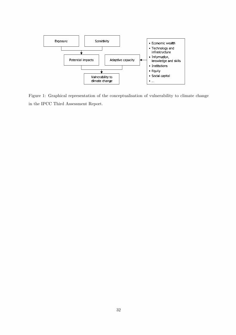
Figure 1: Graphical representation of the conceptualisation of vulnerability to climate change

in the IPCC Third Assessment Report.

32

Symbol Meaning

f : X → Y f is a function defined on the set X and taking values into the set Y

X × Y The set of ordered pairs having as first element an element of X

and as second element an element of Y

x ∈ X x is an element of the set X

f(x) = y The value of f for the element x is y

x ≺ y x is worse than y

X ⊆ Y X is a subset of Y

p ≡ q p is equivalent to q (p is true if and only if q is true)

x ∧ y Logical and, i.e., x is true and y is true

x 6∈ X x is not an element of the set X

iff if and only if

x > y x is greater than y

R+ The set of positive real numbers

∀ x : ... For all x such that ...

∃ x : ... There exists at least one x such that ...

Table 1: Mathematical symbols and their meanings.

33