Embed Size (px)
Citation preview

1
University of Manchester
George Begg Building - Sackville Street, Manchester
Contents
1 Introduction 12
2 RANS and LES equations 16
2.1 Fluid-dynamics problems . . . . . . . . . . . . . . . . . . . . . . . . . . . . . . . . . . . . . . . . . . 16
2.2 Time averaged equations (RANS) . . . . . . . . . . . . . . . . . . . . . . . . . . . . . . . . . . . . . . 17
2.2.1 Bousinnesq tensor . . . . . . . . . . . . . . . . . . . . . . . . . . . . . . . . . . . . . . . . . . 18
2.2.2 Reynolds stress equation models . . . . . . . . . . . . . . . . . . . . . . . . . . . . . . . . . . 19
2.2.3 RANS output . . . . . . . . . . . . . . . . . . . . . . . . . . . . . . . . . . . . . . . . . . . . . 20
2.3 Space filtered equations (LES) . . . . . . . . . . . . . . . . . . . . . . . . . . . . . . . . . . . . . . . 20
2.3.1 Smagorinsky-Lilly SGS model . . . . . . . . . . . . . . . . . . . . . . . . . . . . . . . . . . . . 21
2.3.2 Dynamic SGS model . . . . . . . . . . . . . . . . . . . . . . . . . . . . . . . . . . . . . . . . . 22
2.3.3 LES inlet . . . . . . . . . . . . . . . . . . . . . . . . . . . . . . . . . . . . . . . . . . . . . . . 22
3 Literature review 24
3.1 Recycling methods . . . . . . . . . . . . . . . . . . . . . . . . . . . . . . . . . . . . . . . . . . . . . . 24
3.2 Synthetic turbulence . . . . . . . . . . . . . . . . . . . . . . . . . . . . . . . . . . . . . . . . . . . . . 25
3.2.1 Random generation . . . . . . . . . . . . . . . . . . . . . . . . . . . . . . . . . . . . . . . . . 26
3.2.2 Spectral method - Batten et al. (2004) . . . . . . . . . . . . . . . . . . . . . . . . . . . . . . . 27
3.2.3 Synthetic eddy method - Jarrin et al. (2006) and Jarrin et al. (2009) . . . . . . . . . . . . . . 28
3.2.4 Synthesized turbulent fluctuations - Davidson and Billson (2006) . . . . . . . . . . . . . . . . 29
4 The synthetic eddy method 31
4.1 Box of eddies . . . . . . . . . . . . . . . . . . . . . . . . . . . . . . . . . . . . . . . . . . . . . . . . . 31
4.2 Computation of the velocity signal . . . . . . . . . . . . . . . . . . . . . . . . . . . . . . . . . . . . . 32
4.3 Convection of the eddies . . . . . . . . . . . . . . . . . . . . . . . . . . . . . . . . . . . . . . . . . . . 33
2
CONTENTS 3
4.4 Length scales and the number of eddies . . . . . . . . . . . . . . . . . . . . . . . . . . . . . . . . . . 33
4.5 Summary of method . . . . . . . . . . . . . . . . . . . . . . . . . . . . . . . . . . . . . . . . . . . . . 34
4.6 Mean flow and Reynolds stresses . . . . . . . . . . . . . . . . . . . . . . . . . . . . . . . . . . . . . . 35
4.7 Pressure fluctuations at the inlet . . . . . . . . . . . . . . . . . . . . . . . . . . . . . . . . . . . . . . 37
4.8 SEM adaptation by Pamiès et al. (2009) . . . . . . . . . . . . . . . . . . . . . . . . . . . . . . . . . . 38
5 The divergence free scheme 40
5.1 From vorticity to velocity . . . . . . . . . . . . . . . . . . . . . . . . . . . . . . . . . . . . . . . . . . 41
5.1.1 Derivation 1 . . . . . . . . . . . . . . . . . . . . . . . . . . . . . . . . . . . . . . . . . . . . . . 41
5.1.2 Derivation 2 . . . . . . . . . . . . . . . . . . . . . . . . . . . . . . . . . . . . . . . . . . . . . . 43
5.2 Shape functions . . . . . . . . . . . . . . . . . . . . . . . . . . . . . . . . . . . . . . . . . . . . . . . . 44
5.2.1 Divergence free condition . . . . . . . . . . . . . . . . . . . . . . . . . . . . . . . . . . . . . . 44
5.2.2 Averaging flow and Reynolds stresses with DF-SEM formulation (isotropic turbulence) . . . . 46
5.2.3 Summary of the conditions on shape function . . . . . . . . . . . . . . . . . . . . . . . . . . . 48
5.3 Non-isotropic turbulence . . . . . . . . . . . . . . . . . . . . . . . . . . . . . . . . . . . . . . . . . . . 49
5.3.1 Relation between vorticity and Reynolds stresses . . . . . . . . . . . . . . . . . . . . . . . . . 50
5.3.2 Vorticity stresses . . . . . . . . . . . . . . . . . . . . . . . . . . . . . . . . . . . . . . . . . . . 50
5.3.3 Structured-based model . . . . . . . . . . . . . . . . . . . . . . . . . . . . . . . . . . . . . . . 51
5.3.4 Vorticity calculation from the previous SEM method . . . . . . . . . . . . . . . . . . . . . . . 51
5.4 Current approach for simulating non-isotropic turbulence . . . . . . . . . . . . . . . . . . . . . . . . 52
5.4.1 Reproduction of the normal stresses u′2, v′2 and w′2 . . . . . . . . . . . . . . . . . . . . . . . 53
5.5 Initial testing of the DF-SEM . . . . . . . . . . . . . . . . . . . . . . . . . . . . . . . . . . . . . . . . 55
6 Code_Saturne implementation 58
6.1 Subroutines structure . . . . . . . . . . . . . . . . . . . . . . . . . . . . . . . . . . . . . . . . . . . . 59
6.1.1 Writing RANS solution - usprog.F . . . . . . . . . . . . . . . . . . . . . . . . . . . . . . . . . 60
6.1.2 Definition of input parameters - ussynt.F . . . . . . . . . . . . . . . . . . . . . . . . . . . . . 60
6.1.3 Application of the synthetic turbulence - syntur.F . . . . . . . . . . . . . . . . . . . . . . . . 61
6.1.4 Useful subroutines - sytusu.F . . . . . . . . . . . . . . . . . . . . . . . . . . . . . . . . . . . . 62
6.1.5 Memory management - memsyn.F . . . . . . . . . . . . . . . . . . . . . . . . . . . . . . . . . 63
7 Channel flow result 65
8 Conclusions 70

CONTENTS 4
9 Future steps 72
9.1 DF-SEM . . . . . . . . . . . . . . . . . . . . . . . . . . . . . . . . . . . . . . . . . . . . . . . . . . . . 72
9.2 Code_Saturne . . . . . . . . . . . . . . . . . . . . . . . . . . . . . . . . . . . . . . . . . . . . . . . . 72
9.3 Future work plan . . . . . . . . . . . . . . . . . . . . . . . . . . . . . . . . . . . . . . . . . . . . . . . 73
Abstract
Because of high interest in hybrid RANS/LES simulations and the high importance of the inlet generation method
from RANS to LES, the development of a new divergence free inlet method is here assumed to be fundamental in
order to decrease the developing length which follows any inlet generation. The new method is an improvement
of that of Jarrin et al. (2009), which is a particle based method which introduces fluctuations in the velocity field
using a superimposition of eddies.
Although some limitations are still present in the new method, improved performance compared to the SEM
(Synthetic Eddy Method) in the channel-flows simulations run is achieved: the Cf coefficient shows a shorter
developing length after the inlet (Fig. 7.0.1) and, furthermore, in the DF-SEM (Divergence Free SEM) the error is
always less than 15% of the final value of Cf , and less than 10% after a very short recovery length, whilst the SEM
shows a greater variation during its development.
The new method, furthermore, highlights the importance of the RANS turbulence model chosen: in order to
decrease the influence of the inlet over the solution it is equally important to both reduce the assumptions the
generative method makes, and use turbulence model which better reproduces the turbulent structures and statistics
present in LES simulations.
The present work outlines the background of the SEM approach, and the modification that have been introduced
to enforce the divergence free condition. Initial applications of the new method in a plane channel flow are presented,
and some of the remaining limitation discussed.
5

List of Figures
1.0.1 Hybrid RANS/LES simulation over an airfoil. Note the LES region, concentrated in the most prob-
lematic area for RANS equations . . . . . . . . . . . . . . . . . . . . . . . . . . . . . . . . . . . . . . 14
1.0.2 Scheme of the inlet generation of a channel flow using synthetic turbulence . . . . . . . . . . . . . . 14
3.1.1 Sketch of a LES using a precursor simulation dedicated to the generation of the inflow data . . . . . 25
3.2.1 Modified Von Karman spectrum . . . . . . . . . . . . . . . . . . . . . . . . . . . . . . . . . . . . . . 30
4.7.1 Pressure fluctuation generated in a channel flow . . . . . . . . . . . . . . . . . . . . . . . . . . . . . . 37
4.7.2 Particular of the pressure fluctuations close to the inlet . . . . . . . . . . . . . . . . . . . . . . . . . 37
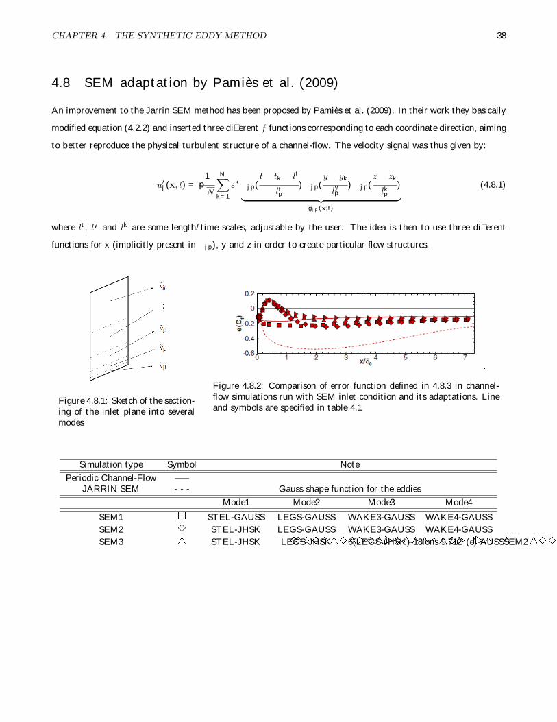
4.8.1 Sketch of the sectioning of the inlet plane into several modes . . . . . . . . . . . . . . . . . . . . . . 38
4.8.2 Comparison of error function defined in 4.8.3 in channel-flow simulations run with SEM inlet condition
and its adaptations. Line and symbols are specified in table 4.1 . . . . . . . . . . . . . . . . . . . . 38
5.2.1 Final shape function chosen for the DF-SEM . . . . . . . . . . . . . . . . . . . . . . . . . . . . . . . 49
5.4.1 Lumley triangle for the DF-SEM. The axes are defined by: 6η2 = b2ii; 6ξ3 = b3ii and bij =<uiuj><ukuk>
�13δij , which is the non-isotropic part of the Reynolds stress tensor. The red line refers to the boundary
limit in turbulence generation:∑3i=1 λi � 2 maxfλ1, λ2, λ3g � 0. The º refers to the DNS of channel
flow performed by Moser et al. (1999). 1C, one-component; 2C, two-components. . . . . . . . . . . . 55
5.5.1 FORTRAN simulation with the described method performed with a Reynolds tensor of
1.5 0.1 0.5
0.1 1.5 0.25
0.5 0.25 1.0
.These pictures clearly show the method capability of reproducing the final Reynolds stresses. Obvi-
ously, the tensor inserted has to satisfy the condition stated in § (5.4.1). . . . . . . . . . . . . . . . . 57
6.1.1 Implementation scheme under Code_Saturne . . . . . . . . . . . . . . . . . . . . . . . . . . . . . . . 59
7.0.1 Comparison SEM and DF-SEM Cf results of a channel flow . . . . . . . . . . . . . . . . . . . . . . . 66
6

LIST OF FIGURES 7
7.0.2 Inlet velocity field generated by DF-SEM . . . . . . . . . . . . . . . . . . . . . . . . . . . . . . . . . 67
7.0.3 Inlet velocity field generated by SEM . . . . . . . . . . . . . . . . . . . . . . . . . . . . . . . . . . . . 67
7.0.4 Velocity field in a fully developed turbulent channel flow performed with LES . . . . . . . . . . . . . 67
7.0.5 Trends of λi and of max(�i)k in the RANS output we used . . . . . . . . . . . . . . . . . . . . . . . . . 68
7.0.6 Reynolds stresses components along the channel flow at y+ � 47 . . . . . . . . . . . . . . . . . . . . 69

List of Tables
3.1 Probability distribution of the random variables . . . . . . . . . . . . . . . . . . . . . . . . . . . . . . 30
4.1 Simulations performed in Channel-flow test case in Fig. 4.8.2. . . . . . . . . . . . . . . . . . . . . . 38
9.2 Gantt chart for my PhD . . . . . . . . . . . . . . . . . . . . . . . . . . . . . . . . . . . . . . . . . . . 73
8
Nomenclature
Roman Symbols
aij Lund coefficient - Cholesky decomposition of the Reynolds stress tensor
B Box of eddies
i Enthalpy
k Turbulent kinetic energy
N Number of eddies
p Pressure
q� Shape function of eddies in the DF-SEM
rk Distance vector between the generic point x and the k-th eddy, located at xk
rk Absolute value of the distance between the generic point x and the k-th eddy, located at xk
RGL Rotational matrix from the reference system L (= local) the the reference system G (= global)
Rij Reynolds stress component. Rij = �ρu′iu′j
T Temperature
t Time
U Vector of mean velocity profile, usually obtained as solution of RANS (time averaged velocity).
u Velocity. It is a vector, function of space and time, of 3 components: (u, v, w)
VB Volume of the eddy box
xk Position of the k-th eddy. It is a vector with 3 components: (xk1 , xk2 , x
k3)
9
LIST OF TABLES 10
Greek Symbols
�k Intensity of the k-th eddy. It is a vector with 3 components: (αk1 , αk2 , α
k3).
In the final method is defined as: αi = Ciεi, and Ci =pk � 2λi
δ Half channel flow height
ε Turbulence dissipation in turbulence modeling
εi Eddy intensity. If used without subscripts see relative statement
λi i-th eigenvalue of the local Reynolds stress tensor.
µ Dynamic molecular viscosity
µt Dynamic eddy viscosity
! Vorticity vector: (ω1, ω2, ω3)
ρ Density
σ Eddy length scale
τij Stress tensor coming from either time averaging operation (RANS) or space filtering (LES)
Subscripts
< φ > Time averaged of the quantity φ. Time averaging may be indicated by φ as well.
φ Temporal averaging or spatial filtering of the quantity φ. The contest will clarify if is an averaging either a
filtering operation. Time averaged may be indicated by < φ > as well
φ′ Fluctuating component of the quantity φ
Acronyms
CFD Computational Fluid-Dynamic
DF-SEM Divergence Free SEM
DNS Direct Numerical Solution
LES Large Eddy Simulation
RANS Reynolds Averaged Navier Stokes

LIST OF TABLES 11
SEM Synthetic Eddy Method
SGS Sub-Grid Scales
Chapter 1
Introduction
Computational fluid-dynamics nowadays plays a major role in design: it saves money and time and, furthermore,
since the beginning of the 20th century when it was first implemented, it has increased continuously its precision
and its accordance with the physics of complex flows. These new features have been allowed by the increasing
computational capability available through more and more powerful processors and by a more developed and accu-
rate flow modelling. Despite this, even today, each algorithm implemented to solve the flow has several limitations
coming either from the model, which may limit the accuracy of the solution in particular area of the flow, or
from hardware limits which may require a long computational time. At the moment two of the most widely used
modelling approaches for engineering flows are:
• RANS equations - time averaged Navier-Stokes
• LES equations - space filtered Navier-Stokes
The RANS equations describe a time averaged flow and model the Reynolds stresses, which are a statistical de-
scription of the turbulence. A large number of RANS models have been proposed and applied to a variety of
industrial problems. However, many of them, particularly the simple ones which are often 2 equations models, do
not perform well in flows including complex physics such as separation and reattachment, huge pressure gradients,
etc. . LES schemes are, in principle, capable to catch such flow features better but require a very high space and
time resolution (particularly close to walls), which means a very high computational time.
Recently, then, hybrid RANS/LES methods have captured the interests of many industries and academic research
programs. These simulations split the domain into several parts and solve RANS equations where they are expected
to give a good representation of the flow field, whilst employing LES in all the other parts, as Fig. 1.0.1 sketches . In
this way it is possible to have the advantages of both RANS and LES approaches and maybe avoid the disadvantages
12


CHAPTER 1. INTRODUCTION 14
Figure 1.0.1: Hybrid RANS/LES simulationover an airfoil. Note the LES region, concen-trated in the most problematic area for RANSequations
Figure 1.0.2: Scheme of the inlet generation ofa channel flow using synthetic turbulence
As stated earlier, all these synthetic turbulence methods are followed by a transition zone where the LES solution
cannot be considered accurate. The dimensions of this zone are influenced mainly by the LES interface and the
way the inlet velocities are generated. Each method makes some assumptions and simplifications to model the
velocity field. As usual then, in order to decrease the transition zone length, we have to improve the physics of the
modelling.
The first consideration about all the synthetic methods mentioned above is that all of them are able to reproduce
the second order statistics imposed by the user (like the Reynolds stresses). However none of them can guarantee a
divergence free velocity field: in fact many authors consider it not to be a mandatory requirement since the coupling
area is typically a 2D plane area. Nevertheless an LES solution concerns both space and time, so there is a relation
between two different time steps which forces us to consider the coupling area as several 2D areas all related, which
substantially makes the problem a 3D problem, and the question of the imposed velocity field satisfying continuity
is, therefore, of relevance.
Fig. 1.0.2 highlights what has just been said: it is possible to consider the inlet creation as a generation of a
synthetic turbulent “channel flow” with a mean zero velocity (basically a 3D volume of a turbulent velocity field
without any mean flow): every time step, a plane of this artificial channel flow is picked and used as an inlet which
couples the RANS and LES solutions. This consideration explains in a very clear way the necessity of the generation
of a divergence free synthetic turbulence.
The new method being developed here is based on the Synthetic Eddy Method (SEM) scheme (a particle
method which uses a superimposition of eddies to represent fluctuations of the velocity field). The introduction of
the divergence free restriction is expected to improve the performance of the method, reducing both the transition
region and the error found in the main flow parameters (for example the Cf ) with respect all the previous methods.

CHAPTER 1. INTRODUCTION 15
The actual DF-SEM (divergence free SEM), as described in chapter § 5, partially achieves the scope here defined,
but showed the importance of an accurate RANS solution: even if the method is able to perfectly reproduce
the RANS velocity field, since this is just a model of the flow field, the transition region may still be present.
Some numerical simulations reported here suggest (see chapter § 7) to use Reynolds stress models rather than
two equations turbulence models: at the moment, anyway, because of method restrictions (see chapter § 5.4.1) no
simulation involving such turbulence model has been performed.
The hidden assumption of all these statements is that if the new DF-SEM is closer to realistic turbulence, then
a shorter transition region should result. Obviously this, at the moment, is an “a priori” assumption, and must be
verified “a posteriori” in tests for a range of industrially relevant cases.
The present work reports, after a short introduction to RANS and LES equations (§ 2), a brief preview of the
most famous synthetic method used (§ 3), stating the most positive and negative feature of each of them. The
SEM is described separately (§ 4) because of its similarity with the new DF-SEM (§ 5), since they are both particle
methods, where eddies define velocity fluctuations. The following chapter (§ 6) describes the implementation of the
method in Code_Saturne, the finite-volume CFD code chosen to test the new method. The last part of the preset
report is about the channel flows performed and their results, compared to the SEM ones (§ 7).
Chapter 2
RANS and LES equations
Since the new method for coupling solutions aims to deal with both RANS and LES equations, it is now necessary
to briefly examine some characteristics of these two different sets of equations, in order to have a better knowledge
and to understand the aspects the DF-SEM must focus on. In the following it is assumed the DF-SEM is dealing
with a hybrid RANS/LES simulation where the RANS equations provide all the data which has to be used to
create the LES inlet conditions. It is then very important to understand all the information available from a RANS
simulations and, obviously, all the parameters needed by the LES solver.
For details of the theoretical part, such as derivation of equations and so on, the reader is referred to the
literature ( Anderson (2001); Pope (2000); Versteeg and Malalasekera (2006))
2.1 Fluid-dynamics problems
A fluid is a physical substance which is capable of flowing. Any dynamic problem related with a fluid becomes
then a fluid-dynamic problem. A physical description of all these problems can be obtained using a set of equations
where each of them describes a particular feature of the fluid problem, for example:
• mass conservation ! continuity equation
• momentum conservation ! momentum equation
• energy conservation ! energy equation
Beyond these equations, it is possible to add others, such as state equations, which characterize the fluid behavior
itself. Usually these are two equations which define relations among the main variables of a fluid (pressure, density,
enthalpy and temperature).
16
CHAPTER 2. RANS AND LES EQUATIONS 17
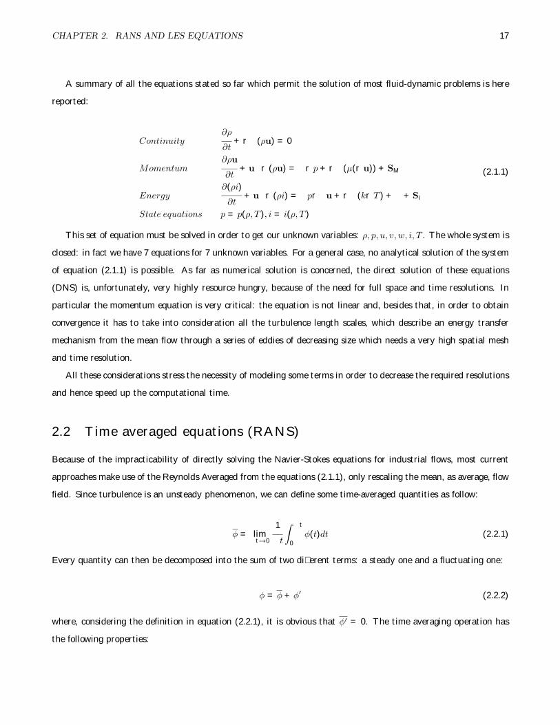
A summary of all the equations stated so far which permit the solution of most fluid-dynamic problems is here
reported:
Continuity∂ρ
∂t+r � (ρu) = 0
Momentum∂ρu
∂t+ u � r(ρu) = �rp+r � (µ(ru)) + SM
Energy∂(ρi)
∂t+ u � r(ρi) = �pr � u +r � (krT ) + � + Si
State equations p = p(ρ, T ), i = i(ρ, T )
(2.1.1)
This set of equation must be solved in order to get our unknown variables: ρ, p, u, v, w, i, T . The whole system is
closed: in fact we have 7 equations for 7 unknown variables. For a general case, no analytical solution of the system
of equation (2.1.1) is possible. As far as numerical solution is concerned, the direct solution of these equations
(DNS) is, unfortunately, very highly resource hungry, because of the need for full space and time resolutions. In
particular the momentum equation is very critical: the equation is not linear and, besides that, in order to obtain
convergence it has to take into consideration all the turbulence length scales, which describe an energy transfer
mechanism from the mean flow through a series of eddies of decreasing size which needs a very high spatial mesh
and time resolution.
All these considerations stress the necessity of modeling some terms in order to decrease the required resolutions
and hence speed up the computational time.
2.2 Time averaged equations (RANS)
Because of the impracticability of directly solving the Navier-Stokes equations for industrial flows, most current
approaches make use of the Reynolds Averaged from the equations (2.1.1), only rescaling the mean, as average, flow
field. Since turbulence is an unsteady phenomenon, we can define some time-averaged quantities as follow:
φ = lim�t→0
1
�t
ˆ �t
0
φ(t)dt (2.2.1)
Every quantity can then be decomposed into the sum of two different terms: a steady one and a fluctuating one:
φ = φ+ φ′ (2.2.2)
where, considering the definition in equation (2.2.1), it is obvious that φ′ = 0. The time averaging operation has
the following properties:

CHAPTER 2. RANS AND LES EQUATIONS 18
• two variables sum: φ+ ψ = φ+ ψ
• constant multiplication: αφ = αφ
• two variables multiplication: φψ = φ ψ + φ′ψ′ (this second term is zero only if φ and ψ are unrelated)
• derivative:∂φ
∂t=∂φ
∂t
• integral:´φds =
´φds
Averaging the continuity and momentum equations (2.1.1), using the stated properties, with the hypotheses of a
steady state, we obtain the famous Reynolds averaged Navier-Stokes (RANS) equations:
Continuity r � (ρ u) = 0
Momentum∂(ρ ui uj)
∂xi= �
∂p
∂xi+
∂
∂xj
µ ∂ui
∂xj+∂uj
∂xi
� ∂
∂xj
(ρu′iu
′j
)+ SM
(2.2.3)
While the continuity equation is mathematically equivalent to the one in (2.1.1), the momentum equation is rather
different: an additional term appears (� @@xj
(ρu′iu′j)). This term involves a 3x3 symmetric tensor (Reynolds stress
tensor), which comes from the convective term. Theoretically it is a very important step: substantially part of
convective term has been moved into the conductive; the Reynolds stresses in fact represent part of the convection
term which the time averaging operation moved to the conductive part. This mathematically stabilizes the equation
and let us use reduced space requirements. On the other hand this tensor adds other 6 unknowns to the problem
which must be modelled in order to provide a final solution of the system. This is the turbulence modelling closure
problem.
2.2.1 Bousinnesq tensor
Bousinnesq proposed in 1877 that Reynolds stresses might be taken as proportional to mean rates of deformation.
It may be written then:
τij = �ρu′iu′j = µt
∂ui
∂xj+∂uj∂xi
� 2
3ρkδij (2.2.4)
where k = 12 (u′2 + v′2 + w′2) is the turbulent kinetic energy per unit mass. The first term of this tensor is exactly
analogous to the viscosity dissipation term, except for the appearance of the turbulent or eddy viscosity µt. The
second term involves δij and it ensures that the formula gives the correct result for the sum of the normal Reynolds
stresses (when i = j). Obviously this representation reduced the unknowns from 6 to only 2: k and µt. There
CHAPTER 2. RANS AND LES EQUATIONS 19
are several turbulence models based on the above assumption, which use different methods to obtain these two
parameters. Here is a brief summary of the most widely used:
• k � ε: adds one equation for k and one for ε. Then µt = ρC�k2
ε, where C� = 0.09.
• k � ω: introduces two equations, for k and for ω. Then µt = ρk
ω.
• k � ω SST : again introduces two equations (k and ω) but takes µt =a1ρk
max(a1ω, SF2), where S =
√2SijSij ,
a1 = const and F2 is a blending function.
• v′2 � f : a turbulence model based on the fluctuation v′2, normal to the walls, which is then valid up to solid
walls. An equation for < v′2 >, together with an equation for the dissipation ε has to be solved. Then
µt = ρC�v′2T , where T = maxfk" , CT (�" )
13 g and both C� and CT are empirical constants.
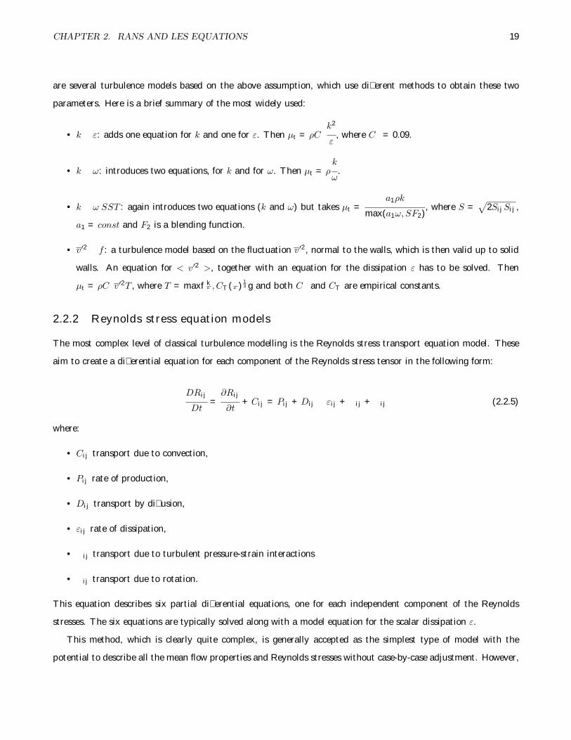
2.2.2 Reynolds stress equation models
The most complex level of classical turbulence modelling is the Reynolds stress transport equation model. These
aim to create a differential equation for each component of the Reynolds stress tensor in the following form:
DRij
Dt=∂Rij
∂t+ Cij = Pij +Dij � εij + �ij + ij (2.2.5)
where:
• Cij transport due to convection,
• Pij rate of production,
• Dij transport by diffusion,
• εij rate of dissipation,
• �ij transport due to turbulent pressure-strain interactions
• ij transport due to rotation.
This equation describes six partial differential equations, one for each independent component of the Reynolds
stresses. The six equations are typically solved along with a model equation for the scalar dissipation ε.
This method, which is clearly quite complex, is generally accepted as the simplest type of model with the
potential to describe all the mean flow properties and Reynolds stresses without case-by-case adjustment. However,

CHAPTER 2. RANS AND LES EQUATIONS 20
such schemes are not as widely validated as the k � ε model and, because of the relatively high cost of the
computations, it is not so widely used in industrial flow calculation.
2.2.3 RANS output
The main results of a RANS simulation are steady values for velocity, pressure, density and the Reynolds stresses.
These values can be used to generate part of the inlet of an LES, but obviously they need the addition of fluctuating
quantities, which are statistically represented by the Reynolds stress tensor. It is important to keep in mind that
this tensor is modelled: RANS models aim to describe its behavior, but they do not have the instruments or the
capabilities to exactly reproduce its physic and its characteristics in all the flows.
From the Reynolds stress tensor, one can of course calculate some more turbulent parameters, such as the
turbulent kinetic energy k′ = u′2 + v′2 + w′2, which can be calculated as follows: k′ = Rkk.
2.3 Space filtered equations (LES)
In order to resolve the largest turbulence energy scales containing eddies, whilst still introducing modelling for the
smallest ones, LES use a set of filtered equations. Spatial filtering operation is defined by means of a filter function
G(x,x′,�) as follows:
φ(x, t) =
ˆ ∞−∞
ˆ ∞−∞
ˆ ∞−∞
G(x,x′,�)φ(x′, t)dx′1dx′2dx′3 (2.3.1)
where φ(x, t) is the filtered function, φ(x, t) is the original unfiltered function, � is the filter cutoff width. In
this section the over-bar indicates spatial filtering, not time-averaging. It is again possible to write:
φ = φ+ φ′ (2.3.2)
In this case, unlike the time averaging, the filter applied to the fluctuating does not always return a zero result:
φ′ 6= 0 (2.3.3)
Obviously many filtering functions G may be applied: top-hat, Gaussian, spectral cut-off. Applying a general
filter to the equations of an incompressible flow we obtain:
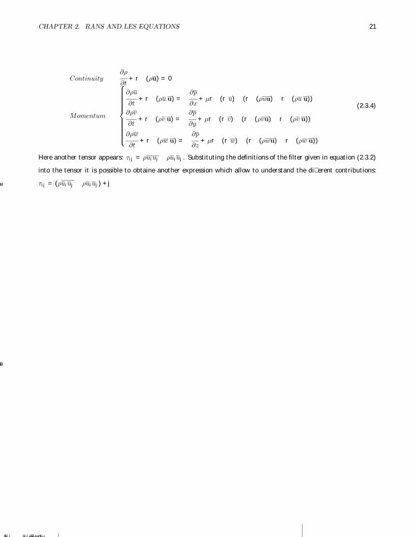
CHAPTER 2. RANS AND LES EQUATIONS 21
Continuity∂ρ
∂t+r � (ρu) = 0
Momentum
∂ρu
∂t+r � (ρu u) = �
∂p
∂x+ µr � (ru)� (r � (ρuu)�r � (ρu u))
∂ρv
∂t+r � (ρv u) = �
∂p
∂y+ µr � (rv)� (r � (ρvu)�r � (ρv u))
∂ρw
∂t+r � (ρw u) = �
∂p
∂z+ µr � (rw)� (r � (ρwu)�r � (ρw u))
(2.3.4)
Here another tensor appears: τij = ρuiuj � ρuiuj . Substituting the definitions of the filter given in equation (2.3.2)
into the tensor it is possible to obtaine another expression which allow to understand the different contributions:
τij = (ρuiuj � ρuiuj) + uiu
j + �
u
2
uj)u
i u
j


CHAPTER 2. RANS AND LES EQUATIONS 23
upstream indefinitely, and so approximate turbulent inlet condition must be specified.
The influence of the inlet boundary conditions on the downstream flow not only depends on the accuracy of the
inflow data, but also on the flow under consideration.

Chapter 3
Literature review
So far, several methods for generating inlet conditions for embedded LES have been proposed. They all aim to
generate an inlet velocity field which does not affect the LES solution significantly. Some of them achieved this
goal, but either with important computational costs or with the requirement of a prior knowledge of the flow field,
which may not be guaranteed in every industrial case.
The scope of this chapter is to give the reader a review of the most widely used inlet generation methods, with
a discussion of their main features, stressing the most positive and negative ones.
3.1 Recycling methods
The most accurate method to specify turbulent fluctuations for a LES or DNS outlet is to run a precursor simulation
whose only role is to provide the main simulation with accurate boundary condition. If the turbulence at the inlet of
the main simulation can be considered as fully developed, periodic boundary conditions in the mean flow direction
can be applied to the precursor simulation. The flow at the outflow plane is then recycled and reintroduced at the
inlet so that the simulation generates its own inflow data. As shown in Fig. 3.1.1, instantaneous velocity fluctuations
from a plane at a fixed stream-wise location are extracted from the precursor simulation and prescribed at the inlet
of the main simulation at each time step. Although no explicit boundary conditions need to be imposed, special care
has to be taken to initialize the flow field properly so that turbulence can be generated as the simulation evolves.
In general, the flow is initialized with a mean velocity profile plus a few unstable Fourier modes - Moser and Rogers
(1992). As already mentioned, periodic boundary conditions can only be used to generate inflow conditions for
flows which are homogeneous in the stream-wise direction, which limits their applications to simple fully developed
flows.
24
CHAPTER 3. LITERATURE REVIEW 25
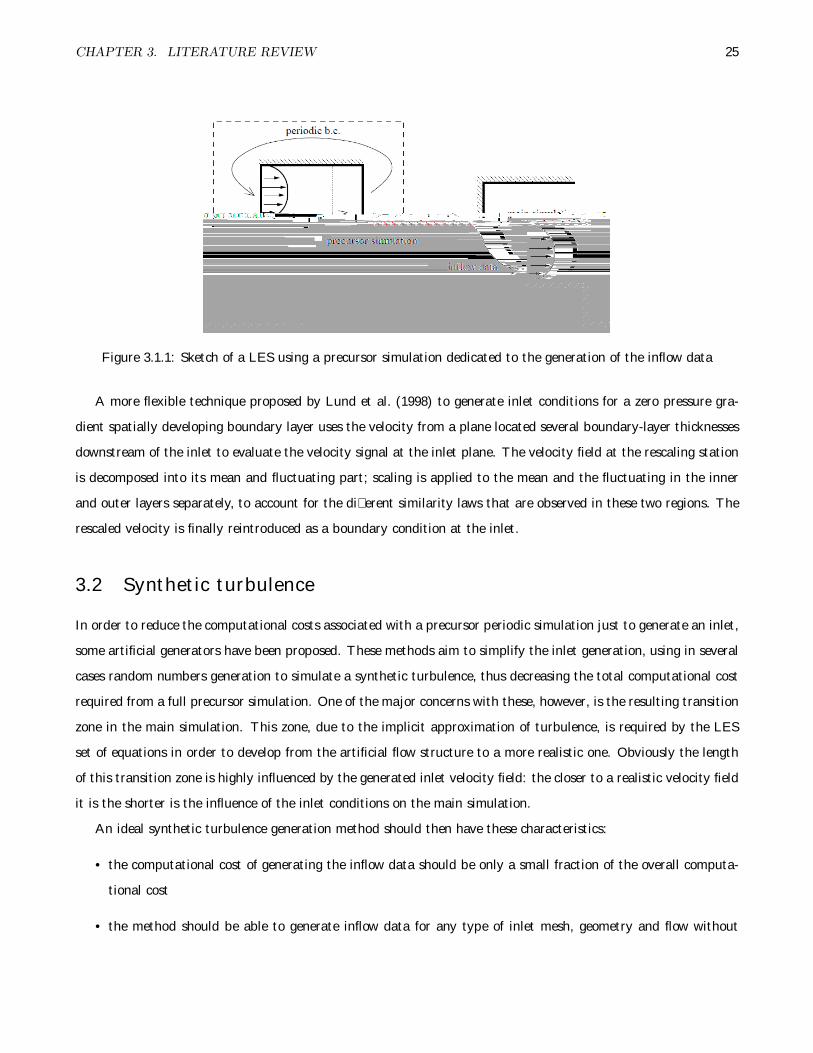
Figure 3.1.1: Sketch of a LES using a precursor simulation dedicated to the generation of the inflow data
A more flexible technique proposed by Lund et al. (1998) to generate inlet conditions for a zero pressure gra-
dient spatially developing boundary layer uses the velocity from a plane located several boundary-layer thicknesses
downstream of the inlet to evaluate the velocity signal at the inlet plane. The velocity field at the rescaling station
is decomposed into its mean and fluctuating part; scaling is applied to the mean and the fluctuating in the inner
and outer layers separately, to account for the different similarity laws that are observed in these two regions. The
rescaled velocity is finally reintroduced as a boundary condition at the inlet.
3.2 Synthetic turbulence
In order to reduce the computational costs associated with a precursor periodic simulation just to generate an inlet,
some artificial generators have been proposed. These methods aim to simplify the inlet generation, using in several
cases random numbers generation to simulate a synthetic turbulence, thus decreasing the total computational cost
required from a full precursor simulation. One of the major concerns with these, however, is the resulting transition
zone in the main simulation. This zone, due to the implicit approximation of turbulence, is required by the LES
set of equations in order to develop from the artificial flow structure to a more realistic one. Obviously the length
of this transition zone is highly influenced by the generated inlet velocity field: the closer to a realistic velocity field
it is the shorter is the influence of the inlet conditions on the main simulation.
An ideal synthetic turbulence generation method should then have these characteristics:
• the computational cost of generating the inflow data should be only a small fraction of the overall computa-
tional cost
• the method should be able to generate inflow data for any type of inlet mesh, geometry and flow without

CHAPTER 3. LITERATURE REVIEW 26
requiring any particular intervention from the user
• the information about the inflow needed for the method to work should be kept as simple as possible (mean
flow, turbulence intensity, RANS statistics, etc.)
• the approximate inflow boundary conditions imposed should have a minimal effect on the flow downstream
of the inlet.
3.2.1 Random generation
The most straight forward approach to generate synthetic fluctuations is to generate a set of independent random
numbers ri taken from a normal distribution @(0, 1) of mean µ = 0 and variance σ = 1 and rescale them such that
the fluctuations have the correct turbulent kinetic energy k; they are then added on to a mean velocity profile U.
The inflow signal thus reads:
ui = Ui + ri
√√√√2
3k (3.2.1)
where the ri are taken from independent random variables for each velocity component at each point and at each
time step. The procedure here illustrated generates a random signal which reproduces the target mean velocity
and kinetic energy profiles. However all cross-correlations between the velocity components and the two-point and
two-time correlations are zero.
An improvement to this method, to correlate the components of the velocity, was proposed in by Lund et al.
(1998). In the case of the Reynolds stress tensor being available, the Cholensky decomposition, aij , of the Reynolds
stress tensor, Rij , can be used to reconstruct a signal which matches the target Reynolds stress tensor. This is done
by taking the velocity signal as:
ui = Ui + rjaij (3.2.2)
where ri are independent random number and aij is given by:
(aij) =
pR11 0 0
R21
a11
√R22 � a2
21 0
R31
a11
(R32 � a21a31)
a22
√
R33 � a231 � a2
32
(3.2.3)
Whilst this method does return prescribed Reynolds stress values, it does not yield any correlations either in
space or in time. In real turbulence, the cascade of energy from large scales to small scales is initiated in the large
scales, which contain most of the energy. The above uncorrelated, random, fluctuations have energy uniformly

CHAPTER 3. LITERATURE REVIEW 27
spread over all wave numbers and thus contain an excess of energy in the small scales which dissipates very quickly.
Klein et al. (2003) noted that using a random method gave the same results as simply imposing a laminar profile at
the inlet nozzle of a turbulent jet. Glaze and Frankel (2003) reported that the random fluctuations they imposed
were almost instantaneously dissipated downstream of the inlet. The turbulent flow was then developed from an
almost laminar inflow profile, which confirms the observations made by Klein et al. (2003). A proposal, suggested
by Klein et al. (2003) was to use a digital filtering procedure to remedy the lack of large-scale dominance in the
inflow data generated by the random method. The main limit to doing so is that a knowledge of time and space
correlations would be required, which makes this method not suitable for practical engineering applications where
little may be known about the inlet flow.
3.2.2 Spectral method - Batten et al. (2004)
This method is based on trigonometric functions. It comes from a statistical view of the velocity field of a turbulent
flow using a Fourier analysis of the velocity spectrum. In this way it is possible to obtain a perfect reproduction of
the time-dependency of the velocity signal, but it is very difficult to reproduce the space dependency.
A set of velocity fluctuations is first defined by:
u′i(x, t) =
√√√√ 2
N
N∑n=1
[pni cos(dnj x
nj + ωnt) + qni sin(dnj x
nj + ωnt)
](3.2.4)
where xj = 2�t�b
and t = 2�t�b
are spatial coordinates normalized by the local turbulent length Lb = k3=2
" and time
scale τb = k/ε. The random frequencies ωn are taken from a normal distribution with mean µ = 1 and variance
σ2 = 1. The amplitudes are given by:
pn = γn � dn, qn = ξn � dn (3.2.5)
where, again, γni and ξni are taken from normal distributions of variance 1 and^dnj = dnj Vb/cnare modified wave-
numbers obtained by multiplying the wave-numbers dni by the ratio of the velocity scale Vb = Lb/τb to cn given
by
cn =
√√√√ 3
2Rlm
dnl dnm
dnkdnk
(3.2.6)
The wave numbers dni are chosen from a normal distribution with zero mean and variance 1/2. Dividing the
wave number by cnelongates those wave-numbers that are most closely aligned with the largest component of the
CHAPTER 3. LITERATURE REVIEW 28
Reynolds stress tensor, and contracts those aligned with the smaller components. This results in a more physically
realistic spectrum of turbulence. The fluctuations are finally reconstructed with the following relation:
ui = Ui + u′jaij (3.2.7)
where aij are the Lund coefficients defined by Lund et al. (1998), and given by equation (3.2.3). These coefficients,
which comes from a Cholensky decomposition of the Reynolds stress tensor, allow us to turn any random velocity
distribution from an isotropic turbulent situation (< u′iu′i >= 1) into a non-isotropic turbulent situations simply
stretching and squeezing the velocity field.
3.2.3 Synthetic eddy method - Jarrin et al. (2006) and Jarrin et al. (2009)
Since a more detailed description of the method may be found in § 4, a short description is here reported.
The SEM method basically defines a box, which is a control volume, and it generates randomly the eddies

CHAPTER 3. LITERATURE REVIEW 29
3.2.4 Synthesized turbulent fluctuations - Davidson and Billson (2006)
This method adds fluctuations to the momentum equations at the interfaces, assuming a modified Von Karman
spectrum. Substantially a turbulent velocity field is simulated using random Fourier modes. This velocity field is
given by:
u′i(xj) = 2
N∑n=1
un cos(κnxj + ψn)σni (3.2.8)
where un, ψn and σni are amplitude, phase and direction of Fourier mode n.
In case of isotropic turbulent fluctuations the procedure is the following one:
1. For each mode n, create random angles φn, αn and θn and a random phase ψn. The probability distributions
employed are given in table 3.1
2. Define the highest wave number based on mesh resolution κmax = 2π/(2�), where � is the smallest grid
spacing at the x� z interface plane
3. Define the smallest wave number from κ1 = κe/p where κe = α9π/(55Lt), α = 1.453. The factor p should be
larger than one to make the largest scales larger than those corresponding to κe
4. Divide the wave number space κmax � κ1into N = 150 modes, equally spaced at intervals of �κ
5. Compute the randomized components of κnj
6. Continuity requires that the unit vectors, σni and κnj are orthogonal. σn3 is arbitrarily chosen to be parallel to
κni , and αn and the requirement of orthogonality then give the remaining two components
7. A modified Von Karman spectrum is chosen (see fig. 3.2.1). The amplitude of each mode is then obtained
from un = (E(jκnj j)�κ)1=2
8. Expression 3.2.8 can be evaluated

CHAPTER 3. LITERATURE REVIEW 30
Probability distribution of the random variablesp(φn) = 1/(2π) 0 � φn � 2πp(ψn) = 1/(2π) 0 � ψn � 2πp(αn) = 1/(2π) 0 � αn � 2πp(θn) = 1/2 sin(θ) 0 � θn � 2π
Table 3.1: Probability distribution of the random variables
Figure 3.2.1: Modified Von Kar-man spectrum
The method is divergence free, but is only able to reproduce isotropic fluctuations. In case a non isotropic
field is required, the algorithm can be modified: the principal coordinate direction of the Reynolds stress tensor
is calculated and fluctuations are generated in this reference system. These are then transformed back into the
original coordinate frame. In this case, however, the method is no longer divergence free, since the Reynolds stress
tensor is not constant all over the domain, leading to different transformations from the local reference system to
the global one at each point.
Chapter 4
The synthetic eddy method
The basic scheme of the new DF-SEM method is substantially similar, and based upon to the SEM method by Jarrin
et al. (2009). They are both particle based methods and they both create a set of eddies with random intensities
which they convect through the inlet plane where the synthetic turbulence will be applied. The main difference
between these two methods is the shape of the eddies. In fact in the DF-SEM, as will be explained in chapter § 5,
the eddies have been modeled in a way which allows them to create a divergence free fluctuating velocity.
It is worth now showing the basic scheme of the two methods, highlighting where the main differences arise. A
most detailed description of the original method may be found in Jarrin et al. (2009).
4.1 Box of eddies
Once the inlet surface has been defined, the SEM creates an eddy box around it where the eddies are convected
in order to produce the fluctuating velocities on the inlet surface. In order to fix this box of eddies a finite set of
points fx1,x2, ...,xsg of R3, on which we want to generate synthetic velocity fluctuation, has to be taken. The mean
velocity U, the Reynolds stresses Rij and a characteristic length scale of the flow σ are assumed to be available on
the set of points considered: details of the estimation of these quantities in case of reduced information available
will be addressed later. The first step is to create a box of eddies B which is going to contain the synthetic eddies.
It is defined by
B = f(x1,x2, ...,xs)εR3, xi;min < xi < xi;max i = f1, 2, 3gg
where
31

CHAPTER 4. THE SYNTHETIC EDDY METHOD 32
xi;min = min(xinlet surface � σ(x))
xi;max = max(xinlet surface + σ(x))
The volume of the box of eddies is noted as VB .
4.2 Computation of the velocity signal
This is the most critical part in both methods. The prescriptions employed in the SEM approach is described below
whilst the modifications introduced to produce a divergence free field will be described later in chapter § (5).
The fluctuating components are calculated using the following equation:
ui = Ui +1pN
N∑k=1
aijεkj f�(x)(x� xk) (4.2.1)
where:
• Ui is the averaged velocity from the RANS solution
• aij are the Lund coefficients, coming from the Cholensky decomposition of the Reynolds stresses tensor and
defined in equation (3.2.3)
• εj are the intensities of the eddy in the j-th direction
• f�(x) is the eddy shape function, which describes the velocity distribution around the eddy centre xk.
Jarrin et al. (2006) suggested as shape function the following one:
f�(x� xk) =√VBσ
−3=2f(x� xk
σ)f(� yk
σ)f(
z � zk
σ) (4.2.2)
where σ is the eddy length scale and f has to satisfy these conditions:
´R f
2(x) dx = 1´ +�
−� f2(x) = 1 (4.2.3)
Among the solutions of the equation here defined, the one suggested by Jarrin et al. (2009) is:
√√√√3
2(1� jxj) jxj < 1
0 otherwise
(4.2.4)

CHAPTER 4. THE SYNTHETIC EDDY METHOD 33
The intensities εj are taken from a random number series with < εj >= 0 and < ε2j >= 1. All these conditions,
together with those on the shape function, come from an analysis of the Reynolds stress generated using this
method, illustrated in chapter § 4.6.
4.3 Convection of the eddies
The position of the eddies, xk, before the first time step are independent from each other and are taken from a
uniform random distribution U(B) over the box of eddies B. The eddies are then convected through the box with
a constant velocity Uc characteristic of the flow. It is straight forward to compute Uc as the bulk velocity over the
set of points S (Uc =´inle surface
U(x) dx). At each iteration, the new position of eddy k is then given by
xk(t+ dt) = xk(t) + Ucdt (4.3.1)
where dt is the time step of the simulation. If an eddy k is convected outside the box through face F of B, then
it is immediately regenerated randomly on the face of B opposite to F with a new independent random intensity
vector εkj still taken from the same distribution.
4.4 Length scales and the number of eddies
The estimation of the length scale of the eddies σ is quite problematic because of the variety of eddies present in
a channel flow and the fact that their structure cannot be represented by a single length scale. In the SST model,
and most other RANS-based schemes, the length scale is given by:
L =k
32
ε(4.4.1)
where ε = C�kω is the case of a ω-based model. For fully developed channel flow in the log-law region, L grows
proportionally to the wall distance. The span-wise integral length scale computed from periodic LES shows a similar
trend as stated by Jarrin et al. (2006). Closer to the wall, for y+ < 50, however, the RANS length scale L tends
towards zero whereas the LES length scale is constant. Several RANS length scales characteristic of the near-wall
region could be defined to clip L in the near-wall region. The Kolmogorov length scale (ν3/ε)1=4 or the viscous
length scale ν/u� appear to be reasonable choices. Neither of these two solutions was adopted by Jarrin et al. (2009)
for robustness reasons, because the correct estimate of the SEM inflow length scale σ was considered too critical
an issue to leave entirely to the RANS model. In fully developed turbulence, the Kolmogorov and viscous length
scales provide a good estimate of the integral length scale in the near wall region, but in the general case, there is
CHAPTER 4. THE SYNTHETIC EDDY METHOD 34
no guarantee that they have any physical relevance. In the case of a free shear flow, or at the reattachment point
of detached flow, for instance, ν/u� is infinite. Instead Jarrin et al. (2009) chose to limit the length scale L by the
local grid spacing � on the LES domain, based on the argument that the LES grid refinement is conditioned by
the size of the near wall structures. The length scale of the eddies is then given by:
σ = max
k 32
ε,�
(4.4.2)
where � = max(�x,�y,�z). The above criterion has the extra advantage of guaranteeing that the synthesized
structures can be accurately discretized on the LES grid. Another region of an attached boundary layer where
RANS predictions become less accurate is the free stream edge. σ was thus limited by an additional geometrical
length scale δ characteristic of the flow under consideration. The final length scale σ used by the SEM is then
computed from:
σ = max
min
k 32
ε, κδ
,�
(4.4.3)
where κ = 0.41.
The aim is to have a LES solution that is not influenced by the specific number of the eddies prescribed at the
inlet. The number of eddies mainly control the intermittency of the synthesized signal. In order to have a constant
flatness in the SEM signal, and hence a LES solution independent of N , the ratio VBN�3 should be constant. The
number of eddies N should then be proportional to VB�3 . For a non-homogeneous distribution of σ, this ratio is also
non-homogeneous in space, and the number of eddies can be computed as:
N = C maxx�B
(VB
σ3) (4.4.4)
where C is a proportionality coefficient to be estimated. This equation ensures that in different situations, the
density of eddies in the inflow, or say the intermittency of the signal is controlled. Now in a given situation, one
wishes to use the minimum value of C which gives rise to a solution independent of N with any further addition of
eddies. Comparing several simulations Jarrin et al. (2009) suggested taking C = 1.
4.5 Summary of method
Finally the different steps in the generation of a velocity signal with the SEM can be summarized:
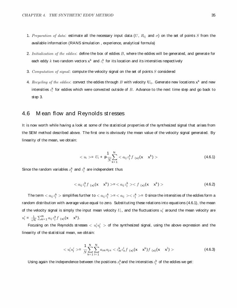
CHAPTER 4. THE SYNTHETIC EDDY METHOD 35
1. Preparation of data: estimate all the necessary input data (U , Rij and σ) on the set of points S from the
available information (RANS simulation , experience, analytical formula)
2. Initialization of the eddies: define the box of eddies B, where the eddies will be generated, and generate for
each eddy k two random vectors xk and εki for its location and its intensities respectively
3. Computation of signal : compute the velocity signal on the set of points S considered
4. Recycling of the eddies: convect the eddies through B with velocity Uc. Generate new locations xk and new
intensities εki for eddies which were convected outside of B. Advance to the next time step and go back to
step 3.
4.6 Mean flow and Reynolds stresses
It is now worth while having a look at some of the statistical properties of the synthesized signal that arises from
the SEM method described above. The first one is obviously the mean value of the velocity signal generated. By
linearity of the mean, we obtain:
< ui >= Ui +1pN
N∑k=1
< aijεkj f�(x)(x� xk) > (4.6.1)
Since the random variables xkj and εkj are independent thus
< aijεkj f�(x)(x� xk) >=< aijε
kj >< f�(x)(x� xk) > (4.6.2)
The term < aijεkj > simplifies further to < aijε
kj >=< aij >< εkj >= 0 since the intensities of the eddies form a
random distribution with average value equal to zero. Substituting these relations into equations (4.6.1), the mean
of the velocity signal is simply the input mean velocity Ui, and the fluctuations u′i around the mean velocity are
u′i = 1√N
∑Nk=1 aijε
kj f�(x)(x� xk).
Focusing on the Reynolds stresses < u′iu′j > of the synthesized signal, using the above expression and the
linearity of the statistical mean, we obtain:
< u′iu′j >=
1
N
N∑k=1
N∑l=1
aimajn < εkmεlnf�(x)(x� xk)f�(x)(x� xl) > (4.6.3)
Using again the independence between the positions xkj and the intensities εkj of the eddies we get:

CHAPTER 4. THE SYNTHETIC EDDY METHOD 36
< u′iu′j >=
1
N
N∑k=1
N∑l=1
aimajn < εkmεln >< f�(x)(x� xk)f�(x)(x� xl) > (4.6.4)
If k 6= l or m 6= n the random variables εkm and εln are independent and hence < εkmεln >=< εkm >< εln >= 0.
If k = l and m = n, then < εkmεln >=< (εkm)2 >= 1 by definition of the intensities. Hence we can write:
< εkmεln >= δklδmn (4.6.5)
The above result let simplify equation (4.6.3) into:
< u′iu′j >=
1
N
N∑k=1
aimajn< f2�(x)(x� xk) >︸ ︷︷ ︸
I1
(4.6.6)
The Probability Density Function (PDF) of xk is needed in order to compute the term I1. xk follows a uniform
distribution over B hence by definition its probability density function can be written as
p1(x) =
1
VBif xεB
0 otherwise
(4.6.7)
Hence we have
I1 =
ˆR3
p(y)f2�(x)(x� y) dy =
1
VB
ˆB
f2�(x)(x� y) dy (4.6.8)
Using the definitions of B and f�, we obtain that I1 = 1. Finally, substituting the above result into equation
(4.6.6) the cross correlation tensor becomes:
< u′iu′j >= aimajn = Rij (4.6.9)
since aij is the Cholesky decomposition of Rij . Hence the Reynolds stresses of the velocity fluctuations generated
by SEM reproduce exactly the input Reynolds stresses. This result is ensured by the use of the Lund coefficients,
which play a main role in achieving this.
Other statistical results are available in Jarrin et al. (2006), but not reported in this work.

CHAPTER 4. THE SYNTHETIC EDDY METHOD 37
4.7 Pressure fluctuations at the inlet
Important pressure fluctuations when an unsteady inlet conditions were used with LES have been observed. These
pressure fluctuations are stream-wise pressure gradients that affect the whole computational domain. On top of this
pressure gradient small pressure fluctuations are seen which are physical and are due to the turbulent structures.
Furthermore a strong influence of the size of the domain and the time step on the intensity of these pressure
fluctuations was noticed.
Figure 4.7.1: Pressure fluctuation generated in achannel flow
Figure 4.7.2: Particular of the pressure fluctuationsclose to the inlet
The origin of these unphysical pressure fluctuations was found to be the fluctuating inlet mass flow rate provided
by the SEM and the Newman boundary condition prescribed on the pressure at the inlet. Since the mass flow rate
fluctuates in time, the Poisson equation has a source term on the right hand side which is very high (due to global
compressibility effect in the stream-wise direction) in the first layer of cells next to the inlet plane. The Laplacian
equation for the pressure with the Newman boundary conditions, reacts in a way that propagates a pressure gradient
to compensate for this source term instantaneously over the whole computational domain. So, three solutions were
suggested by the previous work of N. Jarrin and, so far, none of them is preferred to any other:
1. Applying the SEM on v and w (cross-stream components) and taking u = U0
2. Applying the SEM with a constant mass flow rate, by evaluating Min =´Sρu � ds and then scaling the
fluctuations u = fu with f =MrefMin
3. Applying the SEM with p = 0 at the inlet

CHAPTER 4. THE SYNTHETIC EDDY METHOD 39
This method is definitely able to generate more accurate structures than the old SEM, but its intrinsic problem
is the need for user intervention in prescribing appropriate functions �, � and for the particular flow being
examined. In Fig. 4.8.2, taken from the paper mentioned, a comparison between the SEM and some adaptations
are illustrated. e(Cf ) is defined as the error of the resulting Cf with the analytical form calculated in equation
(4.8.2).
1
2CSf = 0.0225
U∞δ(x)
ν
−1=4
(4.8.2)
e(Cf ) =Cf (x)� CSf (x)
CSf (x)(4.8.3)
To perform the standard SEM simulation a Gaussian distribution function is chosen in equation (4.2.2). The
adaptations are instead performed splitting the inlet into 4 modes and using different functions in each of them, as
described in table 4.1. In order to better understand the function chosen and the method implemented, the reader
is referred to Pamiès et al. (2009).
These results clearly show the higher accuracy that may be reached in such a simulation: the recovery length of
the friction coefficient is in fact highly decreased, but to achieve this goal the method had been tuned for a channel
flow simulation. To get such a tuning a massive user intervention is required and a huge amount of information must
be used. Pamiès et al. (2009) used results coming from previous DNS / LES simulations or experimental results.
This is then the main limit of this method: an user impact, requiring detailed knowledge of the flow characteristics,
is required and this contrasts what we aim for (creating a general method, available for a wide range of cases, and
which does not require any particular user intervention).
Chapter 5
The divergence free scheme
As described in chapter § 4, the SEM scheme uses some randomly positioned eddies to generate inlet conditions for
the LES. It is able to reconstruct the whole Reynolds stress tensor using the Lund coefficients defined in equation
(3.2.3). The equation which allows us to reproduce the velocity field from the eddies distribution is:
ui = Ui +1pN
N∑k=1
aijεkj f�(x)(x� xk) (5.0.1)
In this equation, Ui is the averaged velocity from the RANS solution, aij are the Lund coefficients, coming from
the Cholensky decomposition of the Reynolds stresses tensor, εj is the intensity of the eddy and f�(x) is the eddy
shape function, which describes the velocity distribution around the eddy centre xk.
We want now to create an alternative form for equation (5.0.1) which, beyond all the feature already included,
could return a divergence free velocity field. The aim is that the new method will be using the same framework as
the SEM described in § 4, but the details of the velocity prescription will be different. The divergence free feature
is required to further reduce the developing length which follows the inlet generation, since any natural flow has
such a feature.
In order to get the new DF-SEM main equation the present work has applied the SEM fluctuation method to the
vorticity field and then transferred this to corresponding velocity fluctuations. Via this route as will be illustrated
later on, a divergence free velocity field can be generated.
This chapter explains how the new divergence free method is obtained and analyzes it. Subsequent chapters
address considerations regarding the Reynolds tensor reconstruction, which was a major concern, and present some
results obtained from a FORTRAN implementation which show the capabilities of the new DF-SEM.
40

CHAPTER 5. THE DIVERGENCE FREE SCHEME 41
5.1 From vorticity to velocity
5.1.1 Derivation 1
In order to get a divergence free velocity field (r�u′ = 0) one of the most efficient ways is suggested by Winckelmans
and Leonard (1993). The method uses the vorticity field and superimposes given fluctuations onto this, similar to
those used in the SEM method. These vorticity fluctuations are given by:
!′(x, t) =
√√√√ 1
N
N∑k=1
�k(t)g�(x� xk
σ) (5.1.1)
Equation (5.0.1) and equation (5.1.1), even though they describe two totally different quantities, have a similar
structure. In fact they both make use of an eddy distribution to calculate the fluctuating components of, respectively,
velocity and vorticity. In equation (5.1.1) �k is the intensity of the k-th eddy (a random variable which has to
satisfy: < αki >= 0 and < (αki )2 >= 1), σ is the eddy length scale and g� is the 3D shape function, which describes
the distribution of vorticity around an eddy at position xk (See section § 5.2 for details). The velocity field is then
computed from !′ as the curl of a stream-function, from solving r2Ψ′ = �!′. Recalling that the Green’s function
for �r2 in an unbounded domain is G(x) =1
4πjxj, one can obtain:
Ψ′(x, t) = G(x) � !′(x, t)
=∑Nk=1G( rk
� )�k(t)
=
√√√√ 1
N
1
4π
∑Nk=1
q�( rk
� )�k(t)
(rk
σ)
(5.1.2)
where rk = x� xk, rk = jrkj =√
(x� xk)2 + (y � yk)2 + (z � zk)2 and * stands for the convolution product. The
velocity is then obtained as
u′(x, t) = r�Ψ′(x, t) =∑Nk=1
√√√√ 1
Nr(G( rk
� ))��k(t)
= �
√√√√ 1
N
1
4π
∑Nk=1
q�( rk
� )
(rk
σ)3
rk
σ��k(t) =
√√√√ 1
N
∑Nk=1 K(rk)��k(t)
=
√√√√ 1
N(K(rk)�) � !′(x, t)
(5.1.3)

CHAPTER 5. THE DIVERGENCE FREE SCHEME 42
where K(r)� = �q�(r)
4πr3r� is the Biot-Savart kernel. The function q�( r� ) is an axisymmetric function derived from
g�, defined in equation (5.1.1), though the following relation:
1
z2
d
dzq�(z) = g�(z) (5.1.4)
This is the final stage of the DF-SEM, since the transformation from vorticity to velocity fields given above answer
that the velocity field satisfies continuity. Equation (5.1.3) can be written as:
u′ =
√√√√ 1
N
N∑k=1
q�( rk
� )
(rk
σ)3
rk
σ��k (5.1.5)
which in components form becomes:
u′ =
√√√√ 1
N
∑Nk=1
q�( rk
� )
(rk
σ)3
1
σ((y � yk)αk3 � (z � zk)αk2)
v′ =
√√√√ 1
N
∑Nk=1
q�( rk
� )
( rk
� )3
1
σ((z � zk)αk1 � (x� xk)αk3)
w′ =
√√√√ 1
N
∑Nk=1
q�( rk
� )
( rk
� )3
1
σ((x� xk)αk2 � (y � yk)αk1)
(5.1.6)
The equations are very similar to the SEM ones (5.0.1), but show one main and very important difference: the Lund
coefficient aij , that permitted us to recreate the Reynolds stress statistics in the synthetic generated velocities, are
missing and cannot be introduced in this final equation (5.1.3) without losing the divergence free condition.
A few remarks should be made at this point:
• the stream-function (5.1.2) is not generally divergence-free. This result is a direct consequence of the fact
that r2Ψ′ = �!′ is solved with !′ not generally being divergence-free
• the velocity field (5.1.3) is divergence-free since it is the curl of a stream-function. Indeed, since x � xk is
orthogonal to (x� xk)��k. At x� xk, the singularity is of removable type so that r � u′ = 0.
As noted by Winckelmans and Leonard (1993), one can reconstruct the divergence-free vorticity field by taking the
curl of the velocity field (5.1.3):

CHAPTER 5. THE DIVERGENCE FREE SCHEME 44
In order to simplify this last equation (5.1.11), we can group some terms into a function K�
(x−xk�
), which basically
takes into account of all the integral in equation (5.1.11). Obviously, we then get exactly the same equation we had
found earlier (equation (5.1.6))
u′(x) =
√1
N
N∑k=1
K�
(x� xk
σ
)��k (5.1.12)
This second derivation, even if it is not as elegant as the previous one, shows in a clearer way the connection
between the velocity and vorticity fields. Further, it clearly shows the divergence free condition applied and its
main consequence: the presence of a cross product the expression for the velocity field. This cross producting is the
most important result of all this discussion and the main difference from the original SEM by Jarrin et al. (2006),
and it is the crucial element which allows the the whole method to give a divergence free velocity field.
5.2 Shape functions
5.2.1 Divergence free condition
So far a number of aspects of this new formulation have been discussed, but there is still an important on not
considered yet: the form of the shape functions. In papers such as Winckelmans et al. (2005) many shape functions
are suggested to solve fluid-dynamic problems, so it is very important to give some consideration and checking of
the properties they should possess.
In order to have a better knowledge of which shape function q�( r� ) may be used in the kernel specified in equation
(5.1.6), first the divergence of equation (5.1.6) is calculated and it is imposed to be zero:
r � u = 0 (5.2.1)
Using a general function q�( r� ), depending on the radius rk =√
(x� xk)2 + (y � yk)2 + (z � zk)2, we get the
CHAPTER 5. THE DIVERGENCE FREE SCHEME 45
following equations:
∂u
∂x=
1pN
∑Nk=1

CHAPTER 5. THE DIVERGENCE FREE SCHEME 48
It is now possible to obtain the whole expression for radius rk in the numerator of equation (5.2.12) by adding and
subtracting the term (x� xk)2:
< u′u′ >=1
N
N∑k=1
< [q�(rk
σ)]2
1
σ2
(x� xk)2 + (y � yk)2 + (z � zk)2 � (x� xk)2
( rk
� )6> (5.2.13)
Finally expression (5.2.13) may be simplified in order to get the formulation (and equivalent ones for < v′v′ >
and < w′w′ >):
< u′u′ > =1
N<∑Nk=1[q�( r
k
� )]2
1
( rk
� )4�
1
σ2(x� xk)2
( rk
� )6
>
< v′v′ > =1
N<∑Nk=1[q�( r
k
� )]2
1
( rk
� )4�
1
σ2(y � yk)2
( rk
� )6
>
< w′w′ > =1
N<∑Nk=1[q�( r
k
� )]2
1
( rk
� )4�
1
σ2(z � zk)2
( rk
� )6
>
(5.2.14)
Since we should generate isotropic turbulence when < (αki )2 >= 1, we have to impose < u′iu′i >= 1. This condition
then becomes a condition on the shape function q�(rk).
5.2.3 Summary of the conditions on shape function
1. q�(r) must be a function of the only distance point-eddy rk
2. Isotropic Reynolds stress tensor:1
N<∑Nk=1[q�( r
k
� )]2[
1
( rk� )4�
1�2 (xi−xki )2
( rk� )6
]>= 1
3. Approaching zero at least as fast as ( rk
� )3: limr→0
q�( rk
� )
( rk
� )3= A( r
k
� )n, A 6= 0 and n � 0
4. Must be continuous, as its derivative: q�( rk
� ) εC2
5. q�( rk
� ) j| rk� |>1= 0
Actually, the last restriction is more for computational efficiency than theoretical. Having a function which is non-
zero over all the domain requires a far longer computational time and, since we want the DF-SEM to be computed

CHAPTER 5. THE DIVERGENCE FREE SCHEME 49
Figure 5.2.1: Final shape function chosen for the DF-SEM
very quickly, we introduce this condition. Anyway this limit is not so restrictive: most functions currently proposed
in the literature do, in fact, satisfy it.
The function currently chosen is built up from the following group of functions:
q�(rk
σ) = B(sin(π
rk
σ))2 r
k
σ(5.2.15)
where B is a constant which has to satisfy the integral condition 2. This choice for q�, which respects all the
conditions stated earlier, has been made because of the simplicity of this function (it is basically one of the simplest
that can be computed which satisfies all the limits).
The final shape function, obtained after the normalization to obtain B, is:
q�(rk
σ) =
√√√√ 15VB
16πσ3(sin(π
rk
σ))2(
rk
σ) (5.2.16)
where the constant comes from the integral of expressions in equation (5.2.14), VB is the volume of the eddy box
and σ is the eddy length scale.
5.3 Non-isotropic turbulence
At this stage the DF-SEM is able to reproduce just an isotropic state of turbulence. Obviously this is a big limit
for the method which needs to be generalized before being used in any application: the method must be able to
fully control the velocity field generation, and particularly it must manage to reproduce all the imposed statistics.
The original SEM solved this problem using the Lund coefficients as defined by Lund et al. (1998): these manage
to turn any velocity distribution with isotropic second order momentum (< u′2 >=< v′2 >=< w′2 >= 1) into
a non-isotropic one by squeezeing and pressing the velocity field in order to match it and the imposed statistics.

CHAPTER 5. THE DIVERGENCE FREE SCHEME 50
Obviously this solution can not be applied to the new DF-SEM otherwise it would not be divergence free anymore,
and the method needs an alternative way of controlling.
During the studies several ways were attempted, based on different physical properties of the flow: each of these
tecniques has some limitation, as explaned later on, which may make it not interesting (or too difficult) according
to the main feature the final DF-SEM needs to have.
Here is provided a short description of the approaches, stressing their most positive and negative sides.
5.3.1 Relation between vorticity and Reynolds stresses
One of the most obvious methods of recreating the Reynolds stress in the method defined in equations (5.1.1)-(5.1.3)
is to use any explicit relation between the Reynolds stresses and the vorticity. This relation would allow us to obtain
information about the vorticity second order statistics and to use then the Lund coefficient at this stage, when they
do not affect the divergence free of the final velocity field. To do this, one needs to relate the second order stress
statistics to those of the fluctuating vorticity. Klewicki (1989) defines the following equation:
∂
∂xj(u′ju
′i) = �εijku′jωk +
1
2
∂
∂xi(u′ju
′j)
The relations, which is obtained by applying the derivatine at the definition of the Reynolds stresses, is not an
explicit relation between the variables (fluctuating velocities and vorticity). No simple and easily useable relation
can be extracted from it.
5.3.2 Vorticity stresses
Another way to apply the Lund coefficients arises after comparing equation (5.1.1) and equation (5.0.1). These two
equations are, substantially, exactly identical but one is referred to the vorticity and the other one to the velocity.
As we have already stated, in equation (5.0.1) it was the Lund coefficients which allow us to recreate the Reynolds
stresses. This Lund coefficient could be then inserted in the vorticity equation (5.1.1) in order to recreate some
vorticity second order moments defined as follows:
R{!}ij =< ωiωj > (5.3.1)
In this way we get a very elegant step towards the solution of our problem, even if a new model of these second
order moments is required. This would require a huge amount of data coming from LES or DNS and experimental
data in order to build up the new model and, obviously, a large amount of time. At the moment, then, it has been
preferred to move to other ways.

CHAPTER 5. THE DIVERGENCE FREE SCHEME 51
5.3.3 Structured-based model
Kassinos et al. (2006) defines a third order tensor Qijk = �u′j∂′i
∂xk, where:
∂′i
∂xi= 0
∂2′i
∂x2n
= �ω′i u′i = εits∂′s
∂xt
(5.3.2)
is substantially a variable depending on the vorticity ω. It is certainly possible to then solve our problem, but
its complexity would increase too much, because Qijk is a third order tensor and needs 27 equation to be found.
Since the synthetic turbulence has to simplify the turbulence generation, we have to forsake this way then.
5.3.4 Vorticity calculation from the previous SEM method
Another attempt tried to obtain a vorticity formulation from the original SEM. In this way it is possible either
to obtain a new formulation of the divergence free method or a different coefficient or modification which could
let reproduce the Reynolds stresses as the Lund coefficients do, but without losing the divergence free of the final
velocity field.
The fluctuating component defined by SEM method are here reported:
u′i =1pN
N∑k=0
3∑j=1
aij(x)εj
f�(x)(x� xk) (5.3.3)
And their derivative for each direction:
∂u′i
∂xl=
1pN
∑Nk=0
∑3
j=1
∂aij(x)
∂xlεj
f�(x)(x� xk) +(∑3
j=1 aij(x)εj
) ∂f�(x)(x� xk)
∂xl
(5.3.4)
These derivatives may be used to calculate the fluctuating vorticity, as shown in equation (5.3.5)
ω′1 =1pN
∑Nk=0f
∑3
j=1
∂a2j(x)
∂x3εj
f�(x)(x� xk) +(∑3
j=1 a2j(x)εj
) ∂f�(x)(x� xk)
∂x3
� ...∑3
j=1
∂a3j(x)
∂x2εj
f�(x)(x� xk) +(∑3
j=1 a3j(x)εj
) ∂f�(x)(x� xk)
∂x2
g(5.3.5)
Since all the chosen shape functions are axisymmetric, we are allowed then to use the following assumption

CHAPTER 5. THE DIVERGENCE FREE SCHEME 52
∂f�(x)(x� xk)
∂x1=∂f�(x)(x� xk)
∂x2=∂f�(x)(x� xk)
∂x3(5.3.6)
Using this simplification, we may rewrite equation (5.3.5)
ω′1 =1pN
∑Nk=0
∑3
j=1
∂a2j(x)
∂x3�∂a3j(x)
∂x2
εj
f�(x)(x� xk) +[∑3
j=1 (a2j(x)� a3j(x)) εj
] ∂f�(x)(x� xk)
∂x2
(5.3.7)
This final result is very interesting, even if it does not provide a way to control the output Reynolds stresses directly.
In fact the divergence free hypothesis used in equation (5.1.3) is not valid for the fluctuating velocities in equation
(5.3.3). Equation (5.3.7) suggests to use both a shape function and its derivative to define the vorticity field (and
hence the divergence free velocity field). Further on in this equation both the Lund coefficient and their derivatives
appear. All together this may be a promising idea, even if it makes the equation more complicated to implement
and compute.
5.4 Current approach for simulating non-isotropic turbulence
In section § 5.2.2 we built a method, defined by equation (5.1.6), which can generate isotropic turbulence, where
all the normal components of the Reynolds stress tensor are equal; however the method needs to be generalized in
order to be able to reproduce a wider variety of turbulent states, as we always have in a general fluid-dynamics
problem.
The way this goal has been achieved is similar to that described by Davidson and Billson (2006). It is always
possible to find a local reference system where < u′u′ >, < v′v′ > and < w′w′ > are non-zero, while all the other
second order statistics (< u′v′ >, < u′w′ > and < v′w′ >) are zero: mathematically it means that is always possible
to find three eigenvalues for any symmetric 3x3 matrix, as the Reynolds stress tensor is. We may then align the
eddies with this local system and use the diagonalized Reynolds stresses to calibrate the intensities of the eddies
(see paragraph § 5.4.1 below).
This method may therefore be summarized as follows:
• calculate the eigenvalues and the eigenvectors of the local Reynolds stress tensor
• generate random intensities in the LOCAL reference system (described by the eigenvectors), with amplitude
set as a function of the eigenvalues (see paragraph § 5.4.1)
• create the transformation matrix LOCAL to GLOBAL using the eigenvectors
CHAPTER 5. THE DIVERGENCE FREE SCHEME 53
• calculate the intensities in the GLOBAL reference system: �G = RGL�L
• use these final intensity in equation (5.1.6): u′ =√
1N
∑Nk=1
q�( rk� )
( rk� )3
rk
� � (�k)G
This small but very important difference does not affect the divergence free property of the scheme, since the only
difference is in the intensity �, which had no limit imposed on it earlier. In fact, the new method basically generates
eddies with the same shapes and features described earlier on, and it simply skews those eddies (a velocity field is
divergence free whatever reference system is chosen).
5.4.1 Reproduction of the normal stresses u′2, v′2 and w′2
The last problem which has to be solved regards obtaining the desired normal stresses. To obtain our purpose we
must apply some simplification to the Reynolds stresses in equation (5.2.10). This equation shows clearly that u′2
is influenced by α2 and α3, multiplied by some geometric coefficients ( (z−zk)2
(rk)6 and (y−yk)2
(rk)6 respectively) and by the
eddy shape function q�(r). Since we imposed the Reynolds stresses to be 1 if < α2i >= 1 by tuning the shape
function, we may assume then that half of the final u′2 is due to < α22 >< [q�( r
k
� )]2 1�2
(y−yk)2
( rk� )6
>, and the rest is
due to < α23 >< [q�( r
k
� )]2 1�2
(y−yk)2
( rk� )6
>. This assumption, which is valid because of the eddies random generation,
lead us to an important result:
< [q�(rk
σ)]2
1
σ2
(y � yk)2
( rk
� )6>=< [q�(
rk
σ)]2
1
σ2
(y � yk)2
( rk
� )6>=
N
2(5.4.1)
We may proceed then in our exemplification of equation (5.2.10) as follow
< u′u′ >=< α2
3 >
2+
< α22 >
2(5.4.2)
Similar relations may obviously be found for the other normal component of the Reynolds stress tensor. It is possible
then to obtain the following system linking < αk1 >, < αk2 > and < αk3 > to the eigenvalues of the Reynolds stress
in the principal axes (λ1, λ2 and λ3)
λ1 =1
2(< α2
2 > + < α23 >)
λ2 =1
2(< α2
3 > + < α21 >)
λ3 =1
2(< α2
1 > + < α22 >)
(5.4.3)

CHAPTER 5. THE DIVERGENCE FREE SCHEME 55
then, a recovery area is required.
A more accurate turbulence model (eg. a stress transport model) is suggested, although, at the present stage,
the DF-SEM may not be able to reproduce the desired high stress anisotropy levels.
Figure 5.4.1: Lumley triangle for the DF-SEM. The axes are defined by: 6η2 =b2ii; 6ξ3 = b3ii and bij =
<uiuj><ukuk>
� 13δij , which is the non-isotropic part of the
Reynolds stress tensor. The red line refers to the boundary limit in turbulencegeneration:
∑3i=1 λi� 2 maxfλ1, λ2, λ3g � 0. The º refers to the DNS of channel
flow performed by Moser et al. (1999). 1C, one-component; 2C, two-components.
5.5 Initial testing of the DF-SEM
A short FORTRAN code has been written in order to check out numerically what here has been found theoretically.
The code implements the creation of an inlet condition over a surface of π� π size, divided into 64 x 64 cells. This
surface has been chosen to match the requirements of speed (the simulation had to be quick in order to provide
results) and of size (the surface had to be big enough to provide some reliable solutions).
All the other parameters required by the simulation were taken to be constant all over the domain:
• velocity u = (10, 0, 0),
• eddy number 500
• σ = 0.5
• time step dt = 0.125σ/u
Fig. 5.5.1 shows the Reynolds stress obtained in a simulation where the following Reynolds stress was imposed:
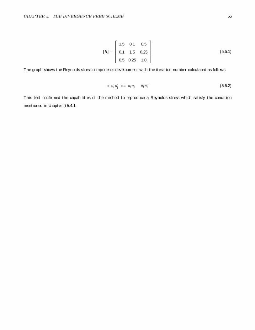
CHAPTER 5. THE DIVERGENCE FREE SCHEME 56
[R] =
1.5 0.1 0.5
0.1 1.5 0.25
0.5 0.25 1.0
(5.5.1)
The graph shows the Reynolds stress components development with the iteration number calculated as follows:
< u′iu′j >= uiuj � uiuj (5.5.2)
This test confirmed the capabilities of the method to reproduce a Reynolds stress which satisfy the condition
mentioned in chapter § 5.4.1.
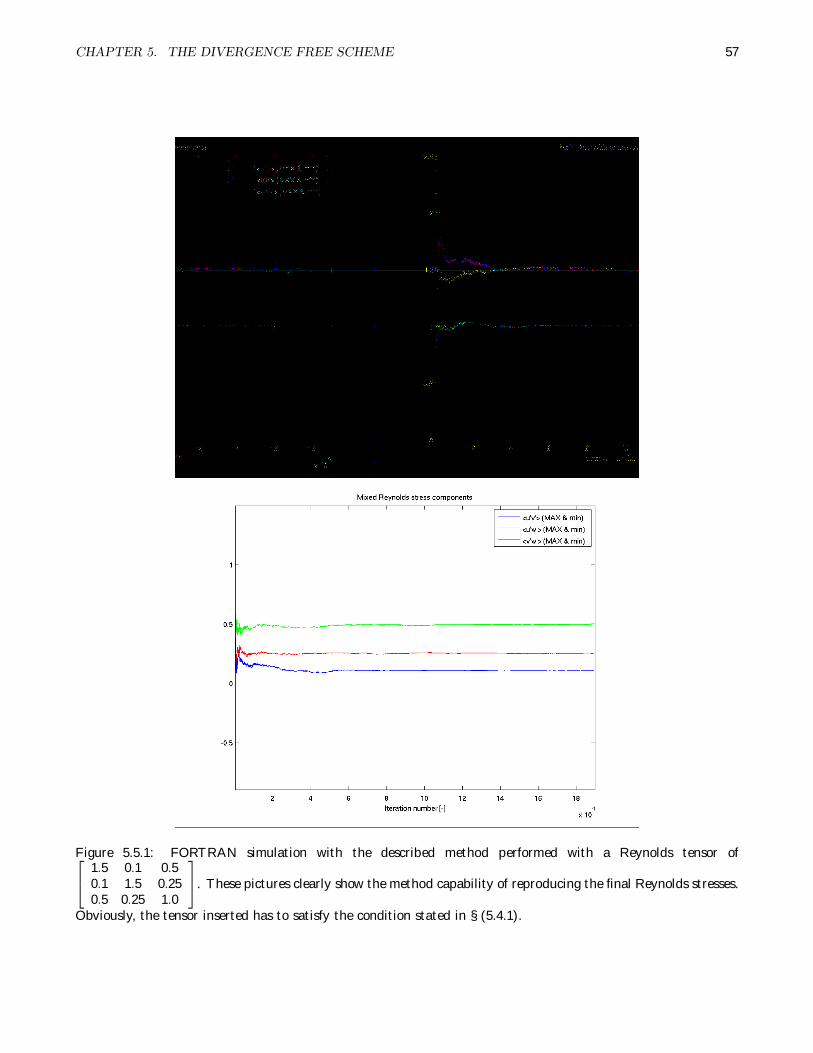
CHAPTER 5. THE DIVERGENCE FREE SCHEME 57
Figure 5.5.1: FORTRAN simulation with the described method performed with a Reynolds tensor of 1.5 0.1 0.50.1 1.5 0.250.5 0.25 1.0
. These pictures clearly show the method capability of reproducing the final Reynolds stresses.
Obviously, the tensor inserted has to satisfy the condition stated in § (5.4.1).

Chapter 6
Code_Saturne implementation
The DF-SEM, as described in Chapter 5, has been implemented in the Code_Saturne CFD software. Code_Saturne
is a software developed by EDF company, based on a finite volume implementation, which is free released via the
company web site.
The aim of this chapter is to provide an overview for the subroutines created in the implementation of the
Divergence Free Synthetic Eddy Method (DF-SEM), together with the SEM and some other models for synthetic
turbulence. The objective of this implementation is primarily the improvement of the SEM approach together with a
benchmark comparison of results with other methods. Furthermore, the project will make these subroutines available
to future users in order to run hybrid RANS/LES simulations; in order to achieve this scope some requirements
must first be fixed:
1. the new subroutines must work with the latest version of Code_Saturne (2.0.0 beta)
2. a synthetic turbulence activation and a memory management part must be introduced
3. any user must be able to perform a hybrid RANS/LES simulations
4. the method must be applicable to any general case and any kind of grid with any number of LES inlets
The subroutines, inserted in the boundary condition definition, use common functions already present and imple-
mented in Code_Saturne, which make them particularly easy to be used by anyone. Further, the user intervention
has been reduced as much as possible, with obvious advantages; at the moment in a normal RANS/LES simulation
the user need only to set a single subroutine as illustrated in § 6.1.
Another desirable feature is that the ease of implementing any new synthetic generation in future is facilitated
by a clear and logical structure. This characteristic will allow some future developers to further the work reported
here.
58
CHAPTER 6. CODE_SATURNE IMPLEMENTATION 59
It should, perhaps be noted that this development remains a work in progress, so many changes may still occur:
while numerical tests in independent FORTRAN code has provided the platform for most of the development to
the code, the Code_Saturne implementation of the DF-SEM has not yet been fully tested across a wide range of
flows. The following sections thus describe the current state of the work in its present form.
6.1 Subroutines structure
The subroutines structure is illustrated in figure 6.1.1. Three main subroutines were created:
• memsyn.F → memory management
• ussynt.F → subroutine which allows the user to set all the synthetic turbulence parameter
• syntur.F → subroutine which applies the synthetic turbulence as a boundary condition at the inlet
Figure 6.1.1: Implementation scheme under Code_Saturne
The implementation method is quite simple. First of all a memory management subroutine is called in caltri.
This subroutine simply specifies and reserves a part of memory for all the data created by the synthetic turbulence
subroutines. Then, at every time step, all the other subroutines are called by tridim for every surface for which an
inlet is required. ussynt defines the surface and the parameters over which syntur, the heart of the synthetic method
generation, has to be applied. These subroutines have already been parallelized: in case more than one processor is
used we decided to perform the eddy creation and convection in one single processor and then broadcast all these
data to all the other processors to perform the inlet generation and application locally. This solution, which is not
the only one possible, has the advantage of spreading the inlet generation over the maximum number of processors,
keeping the communication time quite restricted.

CHAPTER 6. CODE_SATURNE IMPLEMENTATION 60
6.1.1 Writing RANS solution - usprog.F
Standard Code_Saturne subroutine, called every time step
This subroutine is required during the RANS simulation and it is used to output all the data required by the
SEM for the ensuing LES calculation. At the moment the RANS simulation has to be performed before the LES,
which is performed separately subsequently.
output Some dat files a produced with the main variables coming from the RANS. A list with a short description
of the saved data is here reported
post.u.dat - positions and velocities of RANS solution
post.rij.dat - position and Reynolds stresses of RANS solution
post.shear.dat -
lintz_fullinterpol.dat - position and eddy length scale from RANS solution
tintt_fullinterpol.dat -
post.v2f.dat -
This post processing obtains the necessary data from any of the RANS turbulence models available in Code_Saturne.
No limit is the imposed to the user at this point.
6.1.2 Definition of input parameters - ussynt.F
Subroutine called every time step
This is the main subroutine for any user. Once the method is activated in usini1, modifying NSURFSYNTURB
from 0 - standard value - to the number of the surfaces where an LES inlet is required, this subroutine is called
every time step and for each surface. It is essentially a configuring subroutine, where the user has to indicate the
surfaces where the DF-SEM should be generated and it has to link all the data files which must be provided from
a previous RANS solution.
The most important parameters in the subroutine are now described in more detail:
• ISURF: inlet surface index. It identifies the boundary and its range is 0 - NSURFSYNTURB
• SYNTURMETH: it sets the generation method for the ISURF surface. The method available are:
1. No turbulence - application of the RANS velocities at the inlet cells without any fluctuating component
2. Random number - u′ = aijkj , where aij are the Lund coefficients and kj is a random number taken from
a distribution with < k >= 0 and < k2 >= 1.
CHAPTER 6. CODE_SATURNE IMPLEMENTATION 61
3. SEM
4. Batten et al. (2004)
5. DF-SEM
6. Davidson and Billson (2006) (not available yet)
It is possible to generate velocity fields in different ways for each surface, but within any given surface only one
method must be used. Further, in case of restarting a calculation, it is not possible to modify the synthetic
method.
• NRANS(ISURF): it indicates the number of RANS data which has to be read for the ISURF surface.
Beyond these parameters some data generated during the RANS simulation must be read and stored in the RA
array as follows:
• RA(IYRANS + II), where II = 1,2,...,NRANS, must contain all the positions of the points where the velocities
in the RANS simulation are given
• RA(IURANS + II), where II = 1,2,...,NRANS, must contain all the velocities calculated in the RANS
• RA(IRijRANS + II), where i = 1,2,3, j = 1,2,3 and II = 1,2,...,NRANS, must contain all the Reynolds stress
components
• RA(ILijRANS + II), where i = U,V,W, j = X,Y,Z and II = 1,2,...,NRANS, must contain all the eddies length
scale previously calculated.
6.1.3 Application of the synthetic turbulence - syntur.F
Subroutine called every time step
This is a non user adjustable subroutine which implements and applies the synthetic turbulence at the inlet. It
is called every time step and is optimized for the SEM and DF-SEM methods, but it can manage several kinds of
synthetic turbulence.
In case of SEM or DF-SEM all the eddies are created and convected on a single processor only and then these
positions are broadcast to all the other processors (in case of parallelism). Each processor, then, computes its own
velocity field and applies all the computed velocities to its inlet cells. For clarification, this subroutine is divided
into sections:
1. RESTART READING - performed only in case of restart

CHAPTER 6. CODE_SATURNE IMPLEMENTATION 63
where the matrix is stored is defined by the indexes BEGINNING (which defines the area where all the same
genre of matrix are allocated), and ILELT (which defines precisely the location of the matrix linked to the
ILELT-th cell).
• RS ( NM, N, A, W, MATZ, Z, FV1, FV2, IERR) - This is a subroutine which obtains eigenvectors and
eigenvalues from a symmetric matrix. As with all the other matrix management subroutines, this one may
be found in the Netlib Repository. It is called in the DF-SEM in order to align the eddies with the local
Reynolds tensor main reference system.
input NM (rows number), N (columns number), A (matrix), MATZ (=0 to obtain only eigenvalues, =1
to obtain both eigenvalues and eigenvectors)
output W (vector with the eigenvalues), Z (matrix of eigenvectors - the i-th column is one eigenvector),
IERR (error state - a normal simulation returns 0)
others FV1 & FV2 (temporary used vectors)
Further this subroutine requires several other subroutines:
– TRED1 - reduces a real symmetric matrix to a symmetric tridiagonal matrix using orthogonal similarity
transformations.
– TQL1 - finds the eigenvalues of a symmetric tridiagonal matrix by the ql method.
– TRED2 - reduces a real symmetric matrix to a symmetric tridiagonal matrix using and accumulating
orthogonal similarity transformations.
– TQL2 - finds the eigenvalues and eigenvectors of a symmetric tridiagonal matrix by the ql method. The
eigenvectors of a full symmetric matrix can also be found if tred2 has been used to reduce this full matrix
to tridiagonal form.
– PYTHAG - findspa2 + b2 without overflow or destructive underflow.
6.1.5 Memory management - memsyn.F
Subroutine called at the beginning of the simulation and then for every surface where the inlet is applied
This subroutine implements the memory management of the DF-SEM method. It defines the space where all
variables generated by all other subroutines have to be saved; i.e. index definition.
There is also a second subroutine, called SYNIND, contained in the same file. Since the user may define several
inlet surfaces where syntur is applied, we need to have different memory allocation for each of them. The memsyn

CHAPTER 6. CODE_SATURNE IMPLEMENTATION 64
subroutine only allocate the needed memory, but it is synind which, for every surface, sets the indexes. This
subroutine is called every time before ussynt.

Chapter 7
Channel flow result
A channel flow simulation was performed using Code_Saturne 1.4.0 (see § 6) in order to test the methods imple-
mentation and performance.
The channel flow simulated has the following characteristics:
• dimensions: 20π � 2� π
• cell division: 500� 46� 200
• y+ = 1 at the wall cells
• Re� = 395
First of all a 2D RANS simulation of the channel flow was performed, in order to obtain the steady velocity profile
and the Reynolds stress. The turbulence model chosen was the k�ω SST . These data were then used as described
in chapters § 4 and § 5 in order to generate the LES inlet conditions. In order to validate and compare the new
DF-SEM, both an SEM and a DF-SEM simulation were performed.
As suggested by Jarrin et al. (2009), the friction coefficient Cf may be used as a comparison parameter: in
particular considering the recovery length of this parameter to be the distance at which the inlet generation does
not affect anymore the LES. From Fig. 7.0.1 the reader can see the development of the friction coefficient along
the channel flow. This picture shows the DF-SEM has a greater performance compared to the SEM: the initial
drop is limited to 15% of the final Cf , compared to 35% of the SEM. An overshoot is present in both methods: in
the DF-SEM the overshoot is wider but recovered more quickly than the SEM. To summarize: if a 10% error is
accepted, the DF-SEM has a recovery length of about 5d whilst the SEM one is twice longer (aroung 10d).
65

CHAPTER 7. CHANNEL FLOW RESULT 66
Figure 7.0.1: Comparison SEM and DF-SEM Cf results of a channel flow
In order to understand why the channel flow showed these results for Cf , it is now important to compare the
inlet velocities generated by the SEM, the DF-SEM and the velocity field in a fully developed channel flow. Fig.
7.0.2, 7.0.3 and 7.0.4 show snapshots of velocity contour across the channel from both inlet generation methods and
a fully-developed state. The first point to make is the lack of many structures in the SEM approach, compared to
the fully developed one. The DF-SEM seems to better fit the real turbulent structures present in the flow, although
if so far it has not been optimized yet: as stated earlier, exactly the same eddy length scales as defined in the SEM
were used, which may obviously not be optimal for the new method.

CHAPTER 7. CHANNEL FLOW RESULT 67
Figure 7.0.2: Inlet velocity field generated by DF-SEM
Figure 7.0.3: Inlet velocity field generated by SEM Figure 7.0.4: Velocity field in a fully developed tur-bulent channel flow performed with LES
Finally, Fig. 7.0.5 present the computed C coefficients defined in equation (5.4.4). It illustrates the trends of
the three eigenvalues of the Reynolds tensor in the y direction of the channel flow RANS solution. The blue line
is the ratio max(�i)k , which, considering the limit imposed on C, must be confined between 2
3 �max(�i)
k � 1. The
k � ω SST model satisfies this condition, since it is based on the Bousinnesq approximation. As noted earlier,
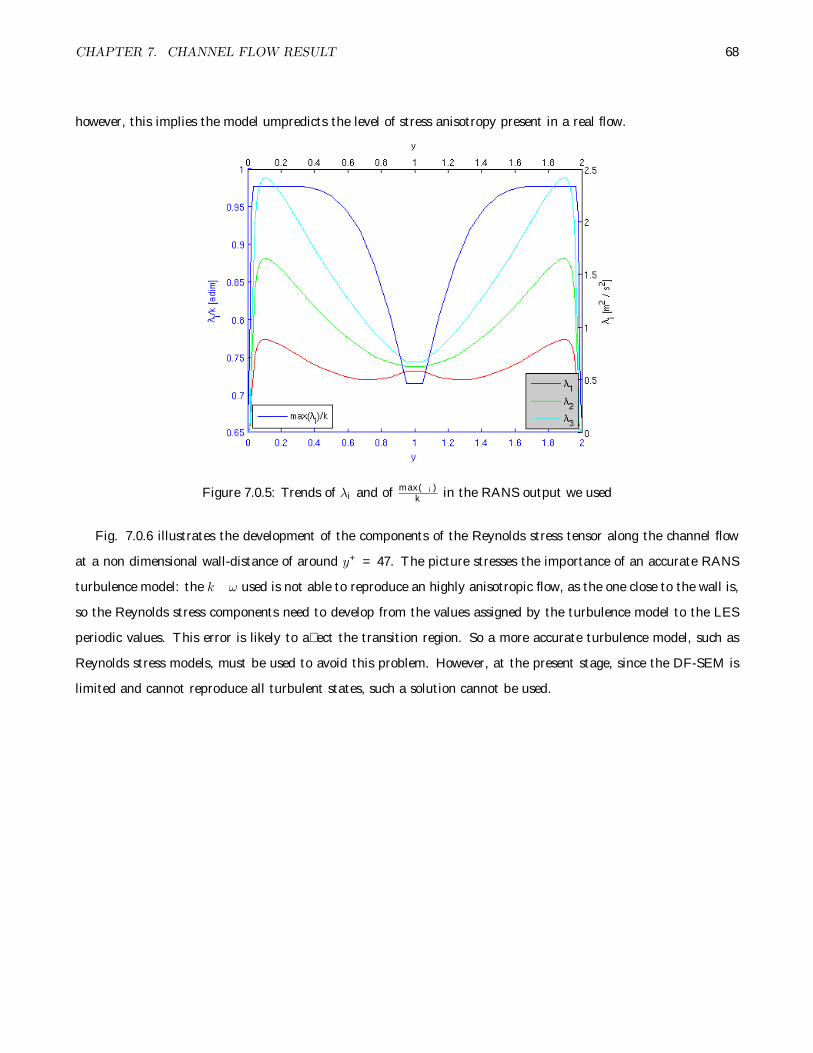
CHAPTER 7. CHANNEL FLOW RESULT 68
however, this implies the model umpredicts the level of stress anisotropy present in a real flow.
Figure 7.0.5: Trends of λi and of max(�i)k in the RANS output we used
Fig. 7.0.6 illustrates the development of the components of the Reynolds stress tensor along the channel flow
at a non dimensional wall-distance of around y+ = 47. The picture stresses the importance of an accurate RANS
turbulence model: the k�ω used is not able to reproduce an highly anisotropic flow, as the one close to the wall is,
so the Reynolds stress components need to develop from the values assigned by the turbulence model to the LES
periodic values. This error is likely to affect the transition region. So a more accurate turbulence model, such as
Reynolds stress models, must be used to avoid this problem. However, at the present stage, since the DF-SEM is
limited and cannot reproduce all turbulent states, such a solution cannot be used.

CHAPTER 7. CHANNEL FLOW RESULT 69
Figure 7.0.6: Reynolds stresses components along the channel flow at y+ � 47
Chapter 8
Conclusions
The SEM method, as defined by Jarrin et al. (2009), is a method which potentially generate synthetic turbulence
and may be used in hybrid RANS/LES simulations. Unlukily, as many other generative methods, it affect the
LES solution because of a transition zone is required after the inlet. The main cause of the transition zone is the
non-divergence-free feature of the method, which leads to a unphysical flow generation.
Here a new solution is proposed, which let the method be divergence free, applying the SEM to the vorticity
and then reobtaining the velocity field. The new method should (only an ’a posteriori’ analisys may confirm that)
be able to reduce the region where the solution is affected by the inlet generation, but, at the present stage, is not
able to reproduce every turbulence state. This limit force the user in the RANS turbulence model choice, which
may not result optimal for a coupled RANS/LES simulation.
The results showed, for a simple channel flow, that the new DF-SEM has higher performarces compared to the
SEM, obviously using the same RANS turbulence model, and in particular it is capable to catch many turbulent
structure of a real flow.
The transition region which follows any inlet method can be seen as composed by many effect. Two of them,
probably the ones which affect the most the result, are:
1. RANS turbulence model
2. Synthetic method assumptions
which basically represent the capability of the RANS method to reproduce the flow and the capability of the
synthetic method to reproduce the RANS solution.
The method here suggested increased considerably the reproducibility of the RANS solutions, in fact higher
performance are achieved compared to SEM method suggested by Jarrin et al. (2009), but at the moment is not
70

CHAPTER 8. CONCLUSIONS 71
able to reproduce every state of turbulence: this limit the user on the choice of the RANS turbulence method,
which basically does not allow to reduce the RANS turbulence model affection to the final solution considerably.
Obviously, many efforts will be focused in solving this problem from now on.

Chapter 9
Future steps
9.1 DF-SEM
The latest version of the DF-SEM seems to be quite promising, despite its limitation in the Reynolds stress recon-
struction, as illustrated in Fig. 5.4.1. Anyway this new synthetic turbulence, since it is closer to the real physics
of the flow than the previous ones, should be able to reduce the transient zone which follows any synthetic inlet
and, because of its divergence free nature, should reduce the pressure fluctuations, which is believed to be related
to the non divergence free peroperty of other generative methods. Only the Code_Saturne implementation and
simulations will give us “a posteriori” results which will confirm these hypotheses.
In the next months efforts will be focused on the implementation of the new method and on running simulations
of some particular test cases, suggested mainly by EDF, possibly to include flow through a T-junction, through a
rod-bundles, or other challenging geometries.
Furthermore, so far we focused mainly on the low order statistics of the DF-SEM, such as the Reynolds stress
tensor. Now, since we have managed to control these statistics, it is possible to develop a deeper knowledge of the
theory related with the DF-SEM: space and time correlations and higher order statistics might be investigated.
These studies are very important to set some parameters, such as the eddy length scale σ and the eddies number
N , which have been chosen so far to be exactly as in the SEM.
9.2 Code_Saturne
The Code_Saturne development is highly linked with the creation of the new method. So far a set of subroutines
has been created for Code_Saturne 1.4.0. Once the method has been tested with these subroutines, we will be
72

CHAPTER 9. FUTURE STEPS 73
able to update to the newer version of the code, which uses FORTRAN 95 rather than FORTRAN 77. The main
difference is the memory allocation, available in the new programming language, which allows one to save memory.
The only passage through Code_Saturne 1.4.0 was forced by the fact that when this work started the newer
version had just been released and it was felt to be better to begin implementation in the earier, more widely-tested,
version. Furthermore this path highlights the memory needed by the new subroutines in a static way, and now it
will be easier to move to an allocatable memory.
9.3 Future work plan
TASKS 2st YEAR 3nd YEAR1 - 3 4 - 6 7 - 9 10 - 12 1 - 3 4 - 6 7 - 9 10 - 12
Implementationof newmethods
(Davidson,...)
x x
Fourieranalysis ofthe velocity
signals
x x
Increase thereproduciblestates of
turbulence inthe DF-SEM
x x x x x x
Second yearreport x x x
Code_Saturne2.0.0 imple-mentation
x x
Feed-back toRANS
equations forhybrid
RANS-LESsimulations(pressure, ..)
x x x x x x
Eventualtests andsimulations
x x x x x x x x x x x
Final PhDthesis x x x x
Table 9.2: Gantt chart for my PhD
Bibliography
Anderson (2001). Fundamentals of aerodynamics.
Batten, P., U. Goldberg, and S. Chakravarthy (2004). Interfacing statistical turbulence closures with Large-Eddy
simulation. AIAA Journal 42 (3), 485–492.
Davidson, L. and M. Billson (2006, December). Hybrid LES-RANS using synthesized turbulent fluctuations for
forcing in the interface region. International Journal of Heat and Fluid Flow 27 (6), 1028–1042.
Germano, M., U. Piomelli, P. Moin, and W. H. Cabot (1991). A dynamic subgrid-scale eddy viscosity model.
Physics of Fluids A: Fluid Dynamics 3 (7), 1760–1765.
Glaze, D. J. and S. H. Frankel (2003). Stochastic inlet conditions for Large-Eddy simulation of a fully turbulent
jet. AIAA Journal 41 (6), 1064–1073.
Jarrin, N., S. Benhamadouche, D. Laurence, and R. Prosser (2006, August). A synthetic-eddy-method for generating
inflow conditions for large-eddy simulations. International Journal of Heat and Fluid Flow 27 (4), 585–593.
Jarrin, N., R. Prosser, J. Uribe, S. Benhamadouche, and D. Laurence (2009, June). Reconstruction of turbulent
fluctuations for hybrid RANS/LES simulations using a Synthetic-Eddy method. International Journal of Heat
and Fluid Flow 30 (3), 435–442.
Kassinos, S., C. Langer, G. Kalitzin, and G. Iaccarino (2006). A simplified structure-based model using standard
turbulence scale equations: computation of rotating wall-bounded flows. International Journal of Heat and Fluid
Flow 27 (4), 653–660.
Klein, M., A. Sadiki, and J. Janicka (2003, April). A digital filter based generation of inflow data for spatially
developing direct numerical or large eddy simulations. Journal of Computational Physics 186 (2), 652–665.
Klewicki, J. C. (1989). Velocity–vorticity correlations related to the gradients of the reynolds stresses in parallel
turbulent wall flows. Physics of Fluids A: Fluid Dynamics 1 (7), 1285–1288.
74

BIBLIOGRAPHY 75
Kraichnan, R. H. (1961). Dynamics of nonlinear stochastic systems. Journal of Mathematical Physics 2 (1), 124–148.
Lee, S., S. K. Lele, and P. Moin (1992). Simulation of spatially evolving turbulence and the applicability of taylor’s
hypothesis in compressible flow. Physics of Fluids A: Fluid Dynamics 4 (7), 1521–1530.
Lund, T. S., X. Wu, and K. D. Squires (1998, March). Generation of turbulent inflow data for Spatially-Developing
boundary layer simulations. Journal of Computational Physics 140 (2), 233–258.
Moser, R. D., J. Kim, and N. N. Mansour (1999). Direct numerical simulation of turbulent channel flow up to
re[sub tau] = 590. Physics of Fluids 11 (4), 943–945.
Moser, R. D. and M. M. Rogers (1992). The three-dimensional evolution of a plane mixing layer: pairing and
transition to turbulence. Journal of Fluid Mechanics 247, 275–320.
Pamiès, M., P.-É. Weiss, E. Garnier, S. Deck, and P. Sagaut (2009). Generation of synthetic turbulent inflow data
for large eddy simulation of spatially evolving wall-bounded flows. Physics of Fluids 21 (4), 045103.
Peyret, R. (200). Introduction to high-order approximation methods for computational fluid dynamics.
Pope (2000). Turbulent Flows.
Versteeg and Malalasekera (2006). An introduction to computational fluid dynamics (the finite volume method).
Winckelmans, G., R. Cocle, L. Dufresne, and R. Capart (2005). Vortex methods and their application to trailing
wake vortex simulations. Comptes Rendus Physique 6 (4-5), 467–486. Aircraft trailing vortices.
Winckelmans, G. S. and A. Leonard (1993). Contributions to vortex particle methods for the computation of
Three-Dimensional incompressible unsteady flows. Journal of Computational Physics 109 (2), 247–273.

BIBLIOGRAPHY 76
Ma io perche’ venirvi? o chi ’l concede?
Io non Enea, io non Paolo sono:
Me degno a cio’ ne’ io ne’ altri crede.
Perche’, se del venire i’ m’abbandono,
Temo che la venuta non sia folle:
Se’ savio, e intendi me’ ch’io non ragiono.1
1Dante’s “Divina Commedia” - Inferno; 2, 31-36