Toward the first quantum simulationwith quantum speedup

Andrew ChildsUniversity of Maryland

Dmitri Maslov Yunseong Nam Neil Julien Ross Yuan Su

arXiv:1711.10980

Simulating Hamiltonian dynamicson a small quantum computer

Andrew ChildsDepartment of Combinatorics & Optimization

and Institute for Quantum ComputingUniversity of Waterloo

based in part on joint work withDominic Berry, Richard Cleve,

Robin Kothari, and Rolando Somma

Workshop on What do we do with a small quantum computer?IBM Watson, 9 December 2013

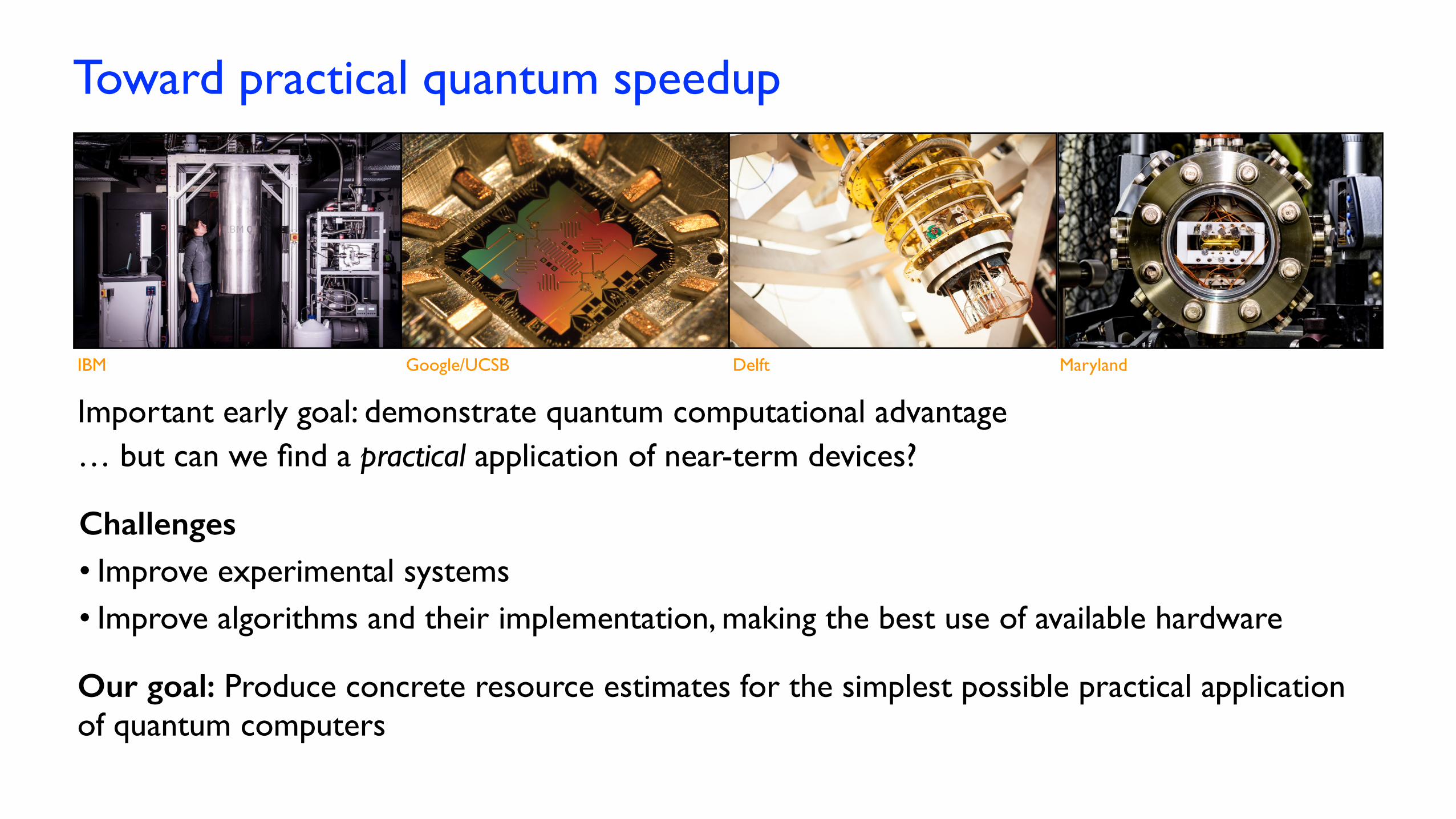
Toward practical quantum speedup

IBM Google/UCSB MarylandDelft

Important early goal: demonstrate quantum computational advantage… but can we find a practical application of near-term devices?

Challenges • Improve experimental systems• Improve algorithms and their implementation, making the best use of available hardware

Our goal: Produce concrete resource estimates for the simplest possible practical application of quantum computers

Quantum simulation“… nature isn’t classical, dammit, and if you want to make a simulation of nature, you’d better make it quantum mechanical, and by golly it’s a wonderful problem, because it doesn’t look so easy.”

Richard Feynman (1981)Simulating physics with computers

Quantum simulation problem: Given a description of the Hamiltonian H, an evolution time t, and an initial state , produce the final state (to within some error tolerance ²)

| (0)i| (t)i

A classical computer cannot even represent the state efficiently.

A quantum computer cannot produce a complete description of the state.

But given succinct descriptions of• the initial state (suitable for a quantum

computer to prepare it efficiently) and• a final measurement (say, measurements

of the individual qubits in some basis),a quantum computer can efficiently answer questions that (apparently) a classical one cannot.

Product formula simulation

[Lloyd 96]

�e�iAt/r

e�iBt/r

�r= e

�i(A+B)t +O(t2/r)

Combine individual simulations with the Lie product formula. E.g., with two terms:

limr!1

�e�iAt/re�iBt/r

�r= e�i(A+B)t

To ensure error at most ², take r = O

�(kHkt)2/✏

�

To get a better approximation, use higher-order formulas.

[Berry, Ahokas, Cleve, Sanders 07]

E.g., second order:

(e�iAt/2re�iBt

e�iAt/2r)r = e

�i(A+B)t

+O(t3/r2)

Suppose we want to simulate H =LX

`=1

H`

Systematic expansions to arbitrary order are known [Suzuki 92]

Using the 2kth order expansion, the number of exponentials required for an approximation with error at most ² is at most

52kL2kHkt⇣

LkHkt✏

⌘1/2k

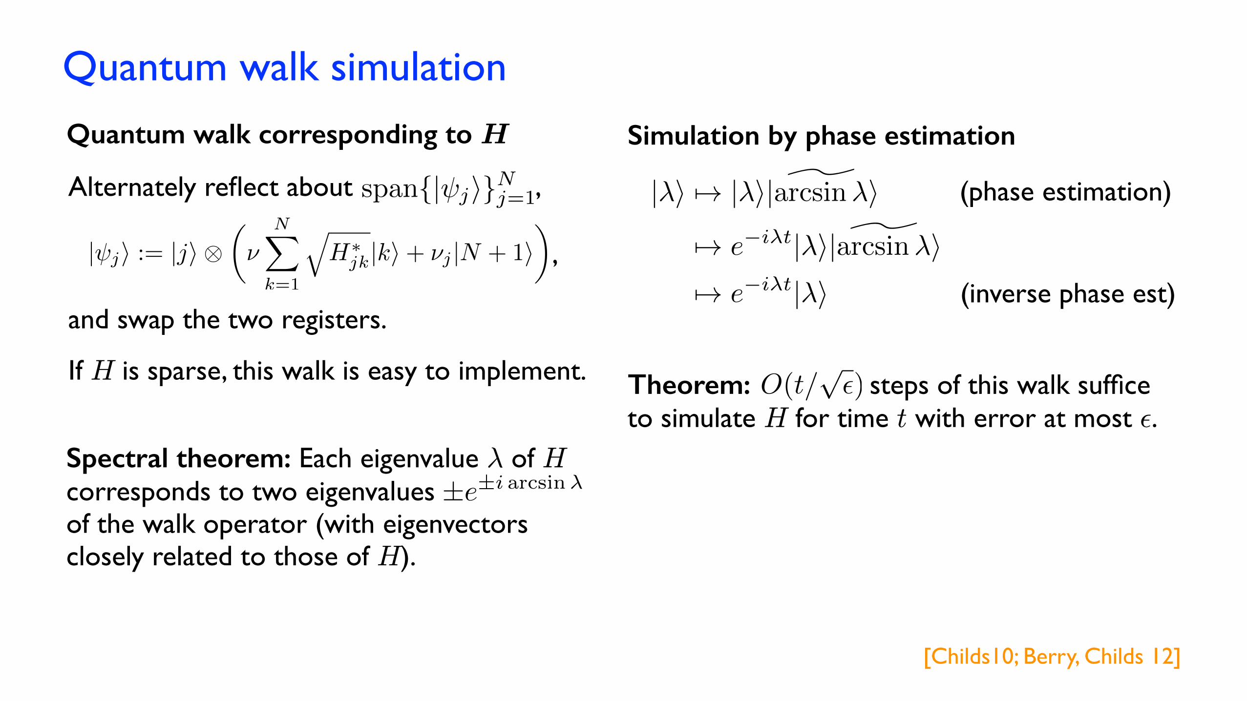
Quantum walk simulation

[Childs10; Berry, Childs 12]

Spectral theorem: Each eigenvalue ¸ of H corresponds to two eigenvaluesof the walk operator (with eigenvectors closely related to those of H).

±e±i arcsin�

Quantum walk corresponding to H

span{| ji}Nj=1Alternately reflect about ,

| ji := |ji ⌦✓⌫

NX

k=1

qH

⇤jk|ki+ ⌫j |N + 1i

◆

and swap the two registers.

,

Simulation by phase estimation

|�i 7! |�i| ^arcsin�i

7! e�i�t|�i| ^arcsin�i7! e�i�t|�i

(phase estimation)

(inverse phase est)

If H is sparse, this walk is easy to implement. Theorem: steps of this walk suffice to simulate H for time t with error at most ².

O(t/p✏)

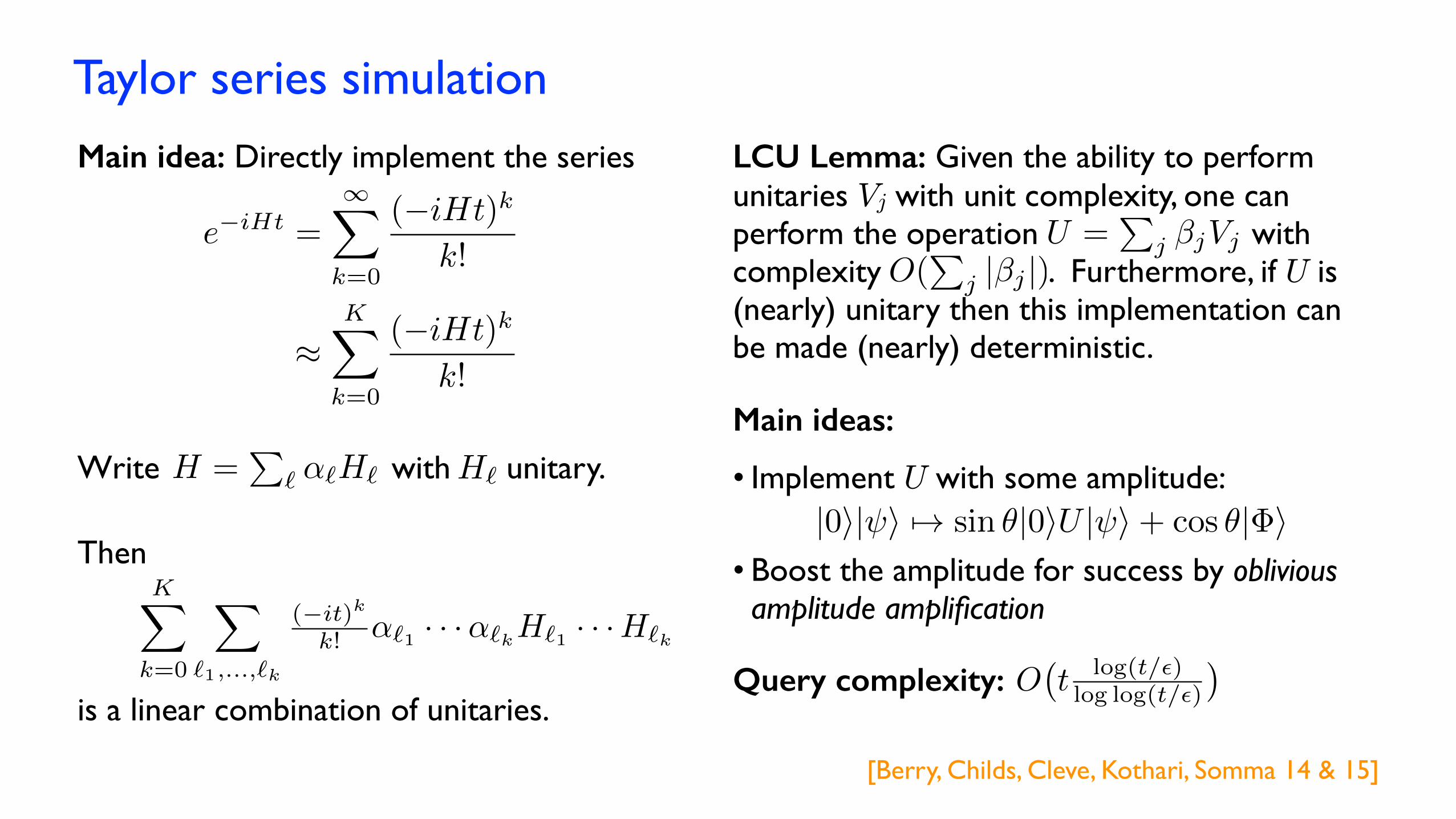
Taylor series simulation

[Berry, Childs, Cleve, Kothari, Somma 14 & 15]

e�iHt =

1X

k=0

(�iHt)k

k!

⇡KX

k=0

(�iHt)k

k!

Write with unitary.H =P

` ↵`H` H`

LCU Lemma: Given the ability to perform unitaries Vj with unit complexity, one can perform the operation with complexity . Furthermore, if U is (nearly) unitary then this implementation can be made (nearly) deterministic.

U =P

j �jVj

O(P

j |�j |)

Main idea: Directly implement the series

Then

is a linear combination of unitaries.

KX

k=0

X

`1,...,`k

(�it)k

k! ↵`1 · · ·↵`kH`1 · · ·H`k

Query complexity: O�t

log(t/✏)log log(t/✏)

�

Main ideas:

• Boost the amplitude for success by oblivious amplitude amplification

|0i| i 7! sin ✓|0iU | i+ cos ✓|�i• Implement U with some amplitude:

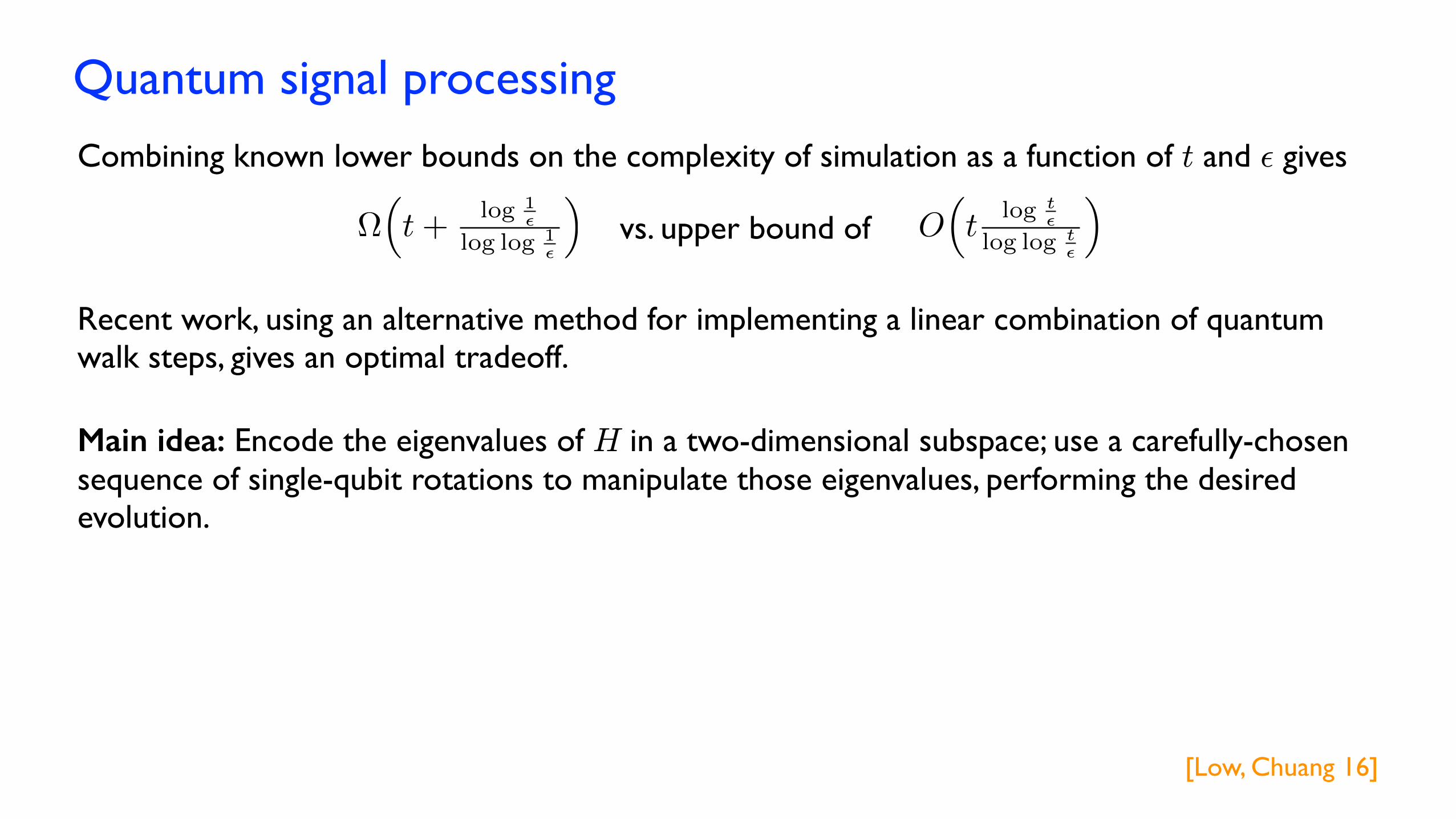
Quantum signal processing

Combining known lower bounds on the complexity of simulation as a function of t and ² gives

⌦⇣t+

log 1✏

log log 1✏

⌘O

⇣t

log t✏

log log t✏

⌘vs. upper bound of

Recent work, using an alternative method for implementing a linear combination of quantum walk steps, gives an optimal tradeoff.

[Low, Chuang 16]

Main idea: Encode the eigenvalues of H in a two-dimensional subspace; use a carefully-chosen sequence of single-qubit rotations to manipulate those eigenvalues, performing the desired evolution.

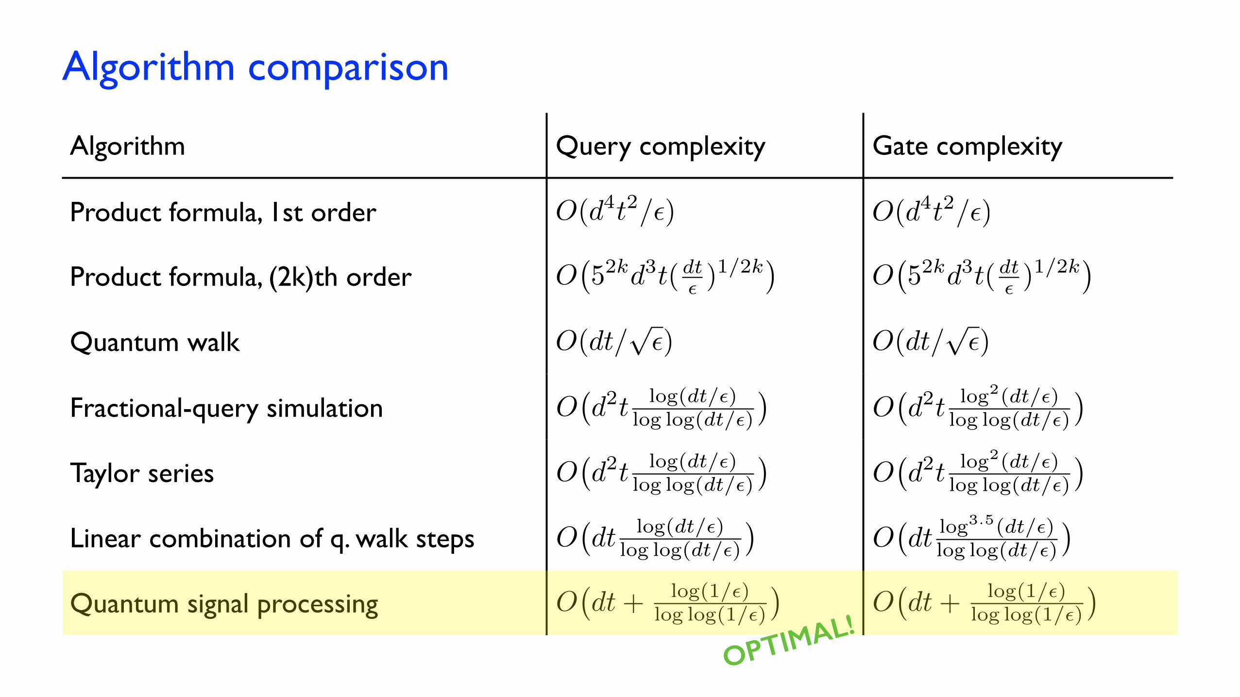
Algorithm comparison

Algorithm Query complexity Gate complexity

Product formula, 1st order

Product formula, (2k)th order

Quantum walk

Fractional-query simulation

Taylor series

Linear combination of q. walk steps

Quantum signal processing

O�d2t

log(dt/✏)log log(dt/✏)

�O�d2t

log2(dt/✏)log log(dt/✏)

�

O(d4t2/✏) O(d4t2/✏)

O�52kd3t(dt✏ )

1/2k�

O�52kd3t(dt✏ )

1/2k�

O�d2t

log(dt/✏)log log(dt/✏)

�O�d2t

log2(dt/✏)log log(dt/✏)

�

O(dt/p✏)

O�dt

log3.5(dt/✏)log log(dt/✏)

�

O(dt/p✏)

O�dt+ log(1/✏)

log log(1/✏)

�O�dt+ log(1/✏)

log log(1/✏)

�O�dt

log(dt/✏)log log(dt/✏)

�

OPTIMAL!

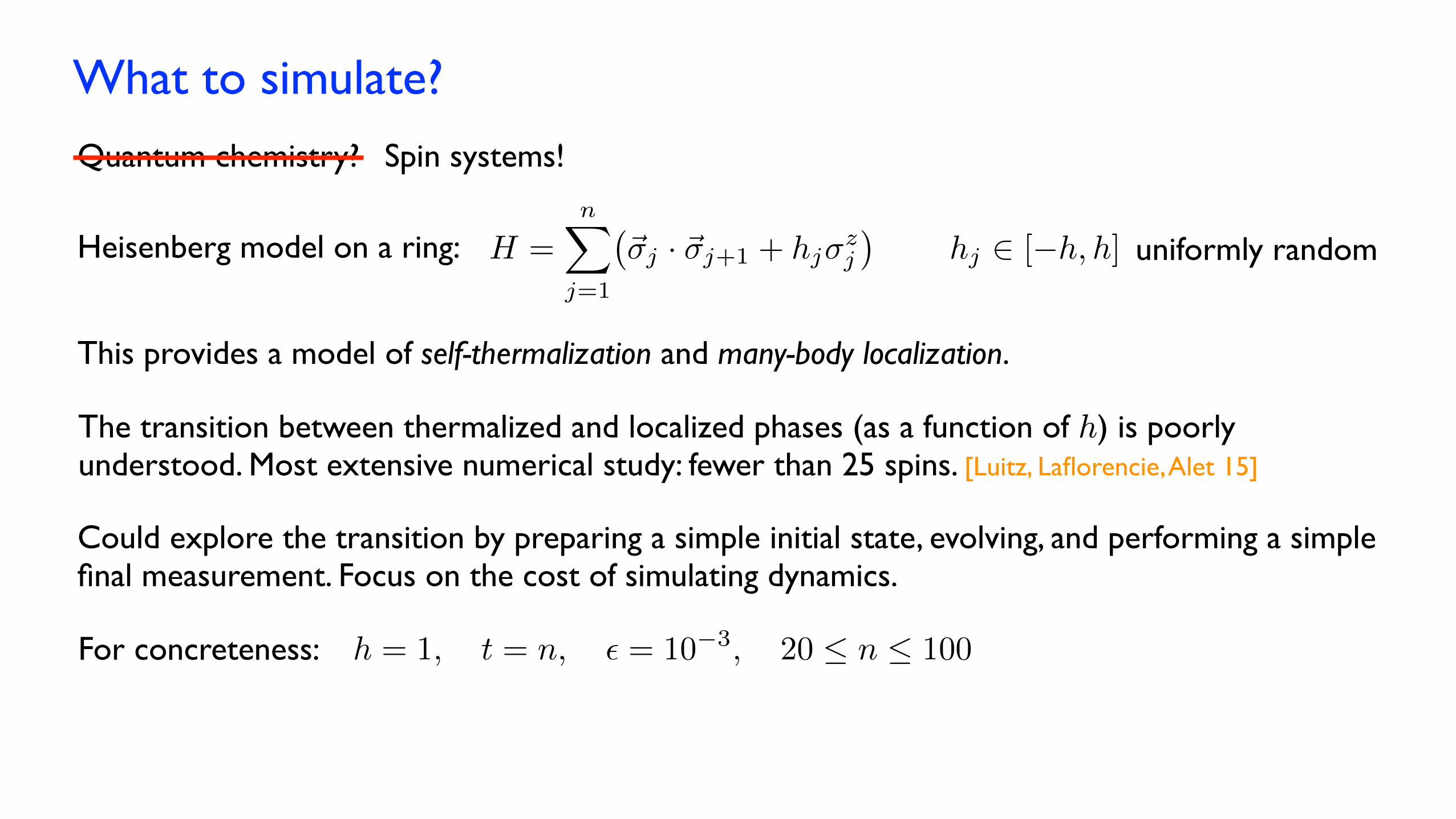
What to simulate?

Quantum chemistry? Spin systems!

Heisenberg model on a ring: H =nX

j=1

�~�j · ~�j+1 + hj�

zj

�hj 2 [�h, h] uniformly random

This provides a model of self-thermalization and many-body localization.

The transition between thermalized and localized phases (as a function of h) is poorly understood. Most extensive numerical study: fewer than 25 spins. [Luitz, Laflorencie, Alet 15]

Could explore the transition by preparing a simple initial state, evolving, and performing a simple final measurement. Focus on the cost of simulating dynamics.

For concreteness: h = 1, t = n, ✏ = 10�3, 20 n 100

Algorithms

Algorithm Gate complexity (t, ²) Gate complexity (n)

Product formula (PF), 1st order

Product formula (PF), (2k)th order

Quantum walk

Fractional-query simulation

Taylor series (TS)

Linear combination of q. walk steps

Quantum signal processing (QSP)

O(t2/✏)

O(52kt1+1/2k/✏

1/2k)

O(t/p✏)

O(n5)

O(52kn3+1/k)

O(n4 log n)

O�t

log2(t/✏)log log(t/✏)

�O�n4 log2 nlog logn

�

O�t

log2(t/✏)log log(t/✏)

�O�n3 log2 nlog logn

�

O�tlog3.5(t/✏)log log(t/✏)

�O�n4 log2 nlog logn

�

O(t+ log(1/✏)) O(n3)

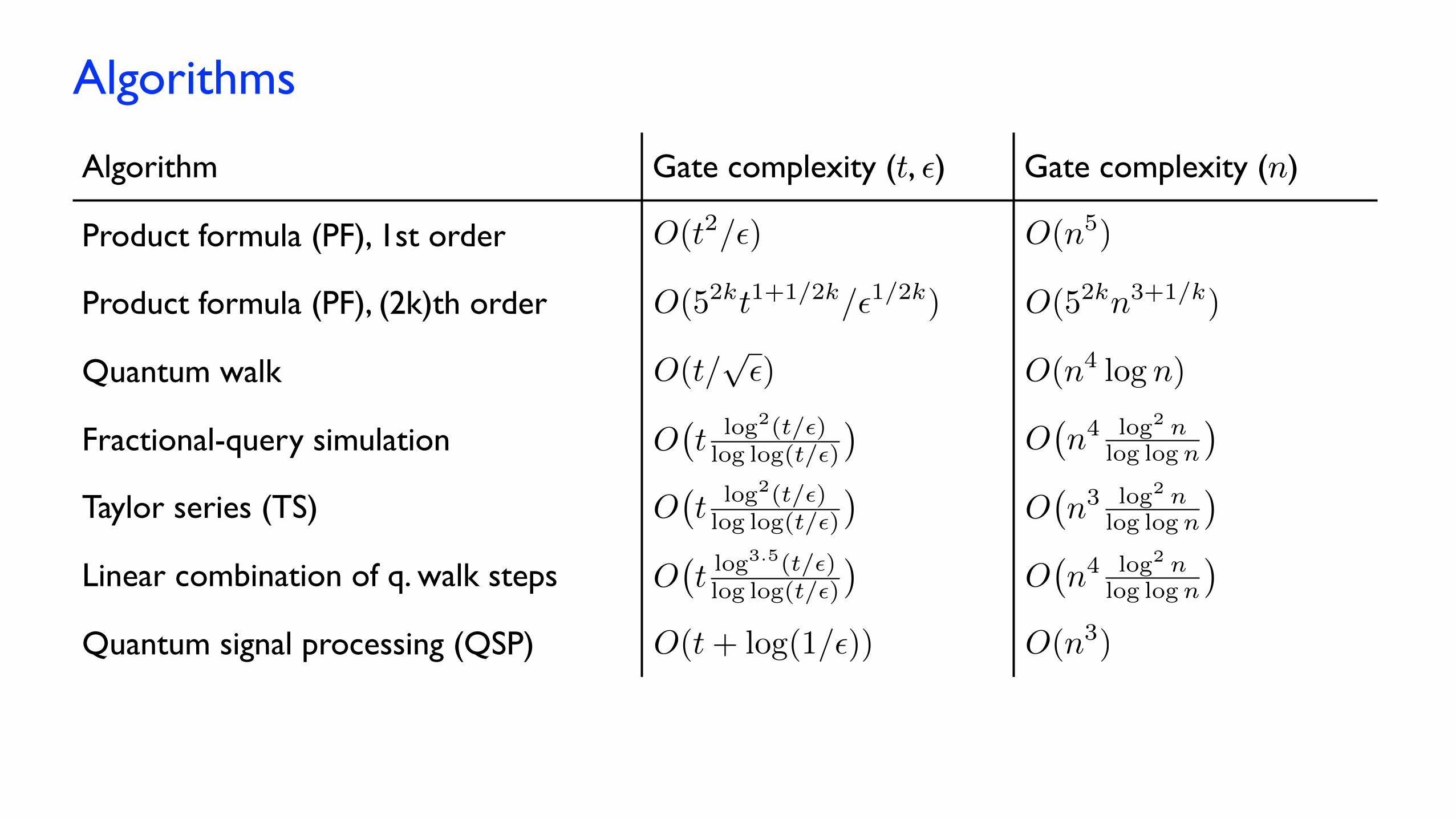
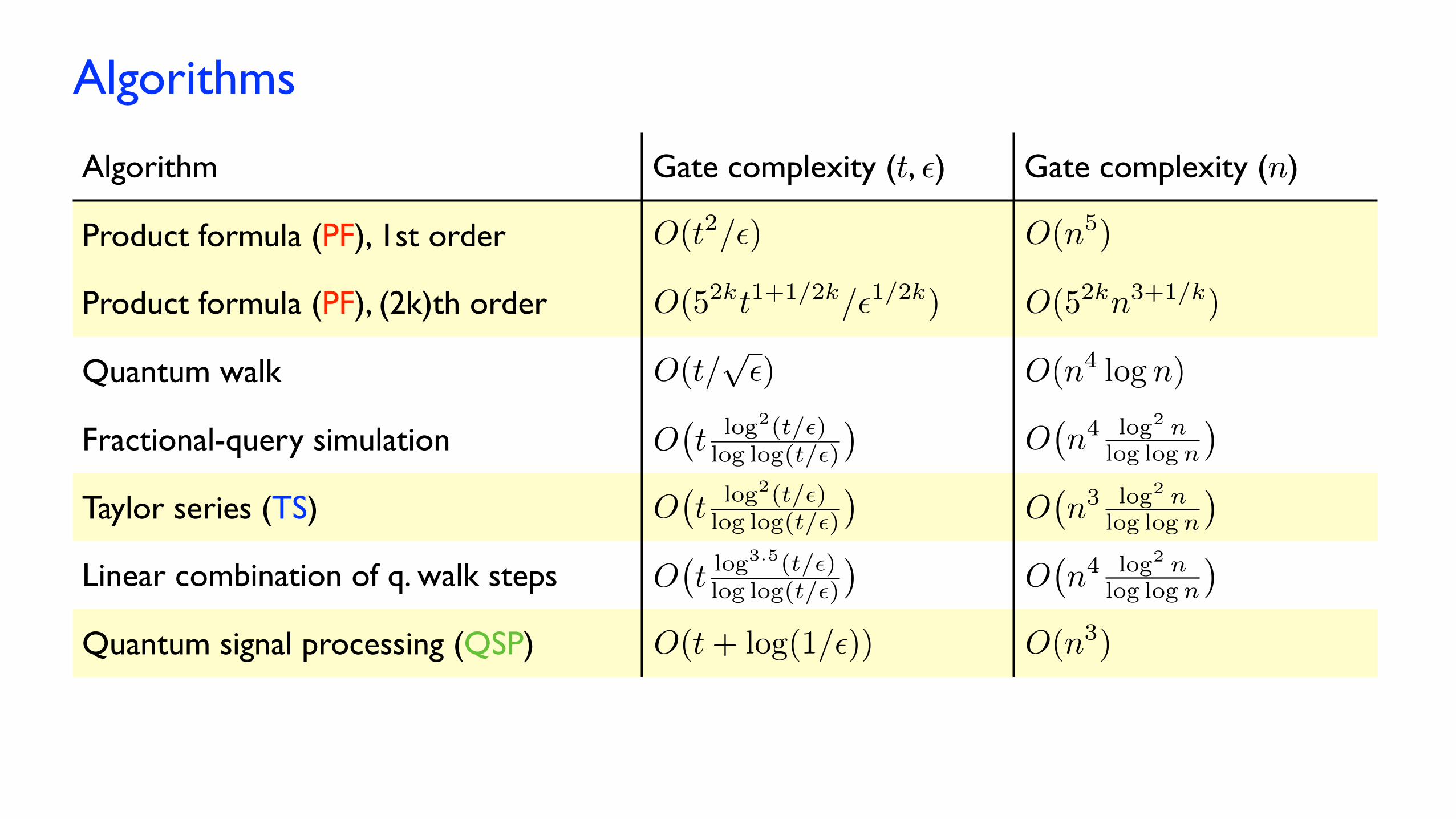
Algorithms

Algorithm Gate complexity (t, ²) Gate complexity (n)

Product formula (PF), 1st order

Product formula (PF), (2k)th order

Quantum walk

Fractional-query simulation

Taylor series (TS)

Linear combination of q. walk steps

Quantum signal processing (QSP)

O(t2/✏)

O(52kt1+1/2k/✏

1/2k)

O(t/p✏)

O(n5)

O(52kn3+1/k)

O(n4 log n)

O�t

log2(t/✏)log log(t/✏)

�O�n4 log2 nlog logn

�

O�t

log2(t/✏)log log(t/✏)

�O�n3 log2 nlog logn

�

O�tlog3.5(t/✏)log log(t/✏)

�O�n4 log2 nlog logn

�

O(t+ log(1/✏)) O(n3)

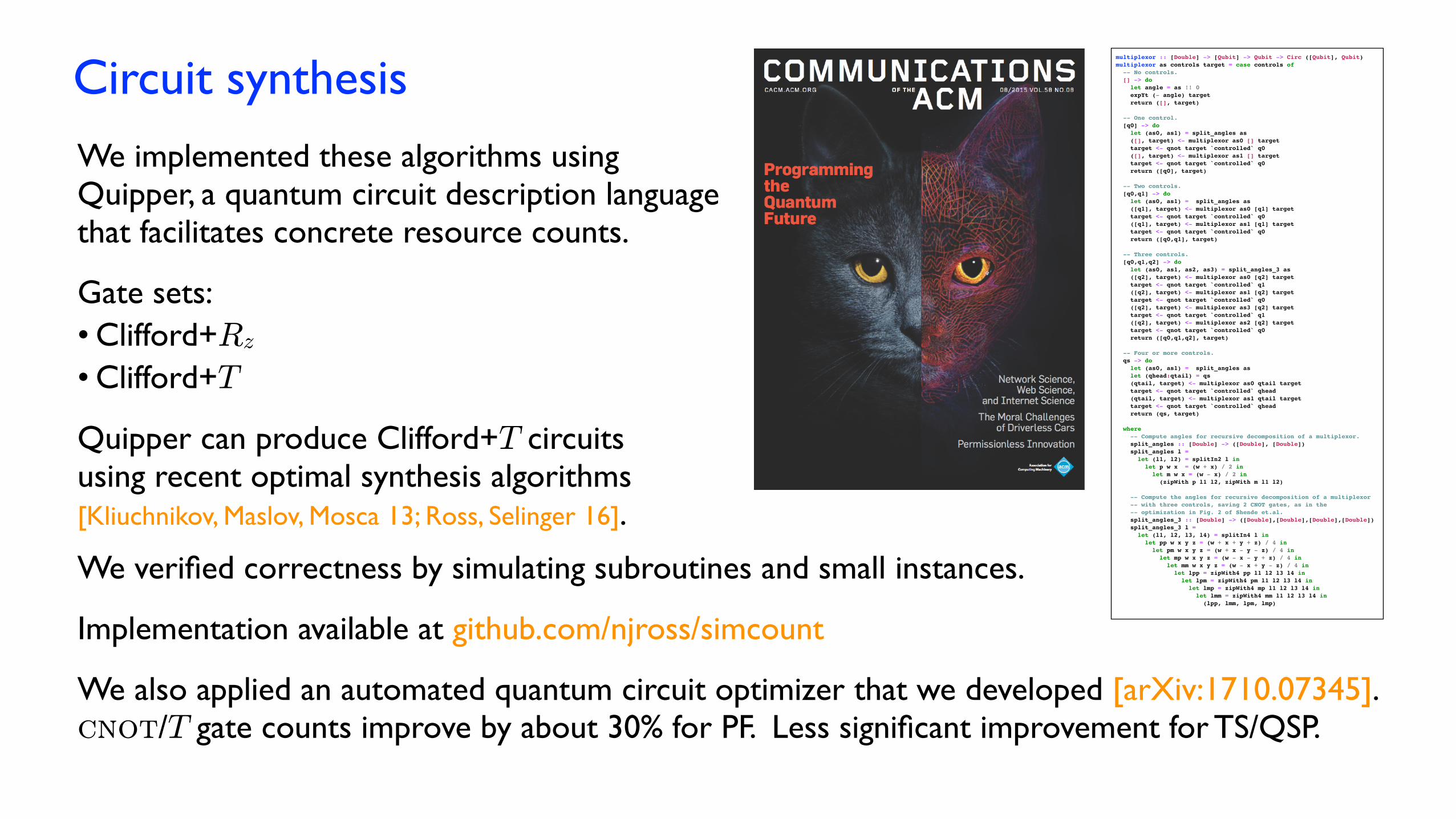
Circuit synthesismultiplexor :: [Double] -> [Qubit] -> Qubit -> Circ ([Qubit], Qubit)multiplexor as controls target = case controls of -- No controls. [] -> do let angle = as !! 0 expYt (- angle) target return ([], target) -- One control. [q0] -> do let (as0, as1) = split_angles as ([], target) <- multiplexor as0 [] target target <- qnot target `controlled` q0 ([], target) <- multiplexor as1 [] target target <- qnot target `controlled` q0 return ([q0], target) -- Two controls. [q0,q1] -> do let (as0, as1) = split_angles as ([q1], target) <- multiplexor as0 [q1] target target <- qnot target `controlled` q0 ([q1], target) <- multiplexor as1 [q1] target target <- qnot target `controlled` q0 return ([q0,q1], target)

-- Three controls. [q0,q1,q2] -> do let (as0, as1, as2, as3) = split_angles_3 as ([q2], target) <- multiplexor as0 [q2] target target <- qnot target `controlled` q1 ([q2], target) <- multiplexor as1 [q2] target target <- qnot target `controlled` q0 ([q2], target) <- multiplexor as3 [q2] target target <- qnot target `controlled` q1 ([q2], target) <- multiplexor as2 [q2] target target <- qnot target `controlled` q0 return ([q0,q1,q2], target)

-- Four or more controls. qs -> do let (as0, as1) = split_angles as let (qhead:qtail) = qs (qtail, target) <- multiplexor as0 qtail target target <- qnot target `controlled` qhead (qtail, target) <- multiplexor as1 qtail target target <- qnot target `controlled` qhead return (qs, target)

where -- Compute angles for recursive decomposition of a multiplexor. split_angles :: [Double] -> ([Double], [Double]) split_angles l = let (l1, l2) = splitIn2 l in let p w x = (w + x) / 2 in let m w x = (w - x) / 2 in (zipWith p l1 l2, zipWith m l1 l2)

-- Compute the angles for recursive decomposition of a multiplexor -- with three controls, saving 2 CNOT gates, as in the -- optimization in Fig. 2 of Shende et.al. split_angles_3 :: [Double] -> ([Double],[Double],[Double],[Double]) split_angles_3 l = let (l1, l2, l3, l4) = splitIn4 l in let pp w x y z = (w + x + y + z) / 4 in let pm w x y z = (w + x - y - z) / 4 in let mp w x y z = (w - x - y + z) / 4 in let mm w x y z = (w - x + y - z) / 4 in let lpp = zipWith4 pp l1 l2 l3 l4 in let lpm = zipWith4 pm l1 l2 l3 l4 in let lmp = zipWith4 mp l1 l2 l3 l4 in let lmm = zipWith4 mm l1 l2 l3 l4 in (lpp, lmm, lpm, lmp)

We implemented these algorithms using Quipper, a quantum circuit description language that facilitates concrete resource counts.

Gate sets:• Clifford+Rz• Clifford+T

Quipper can produce Clifford+T circuits using recent optimal synthesis algorithms [Kliuchnikov, Maslov, Mosca 13; Ross, Selinger 16].

We verified correctness by simulating subroutines and small instances.

Implementation available at github.com/njross/simcount

We also applied an automated quantum circuit optimizer that we developed [arXiv:1710.07345].cnot/T gate counts improve by about 30% for PF. Less significant improvement for TS/QSP.

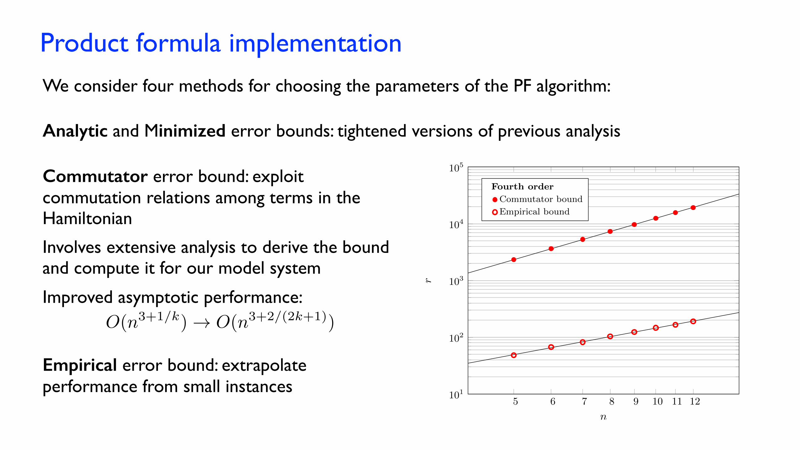
Product formula implementation

Empirical error bound: extrapolate performance from small instances

5 6 7 8 9 10 11 12101

102

103

104

105

nr

Fourth order

Commutator bound

Empirical bound

We consider four methods for choosing the parameters of the PF algorithm:

Analytic and Minimized error bounds: tightened versions of previous analysis

Commutator error bound: exploit commutation relations among terms in the Hamiltonian

Involves extensive analysis to derive the bound and compute it for our model system

O(n3+1/k) ! O(n3+2/(2k+1))

Improved asymptotic performance:

Taylor series implementation

Also give concrete error analysis. Empirical error bounds are infeasible but probably not helpful.

q0

q1

q2

q3

q4

*

x1 x

2 x3 x

4

x1 x

2 x3 x̄

4

x1 x

2 x̄3 x

4

x1 x

2 x̄3 x̄

4

x1 x̄

2 x3 x

4

x1 x̄

2 x3 x̄

4

x1 x̄

2 x̄3 x

4

x1 x̄

2 x̄3 x̄

4

x̄1 x

2 x3 x

4

x̄1 x

2 x3 x̄

4

x̄1 x

2 x̄3 x

4

x̄1 x

2 x̄3 x̄

4

x̄1 x̄

2 x3 x

4

x̄1 x̄

2 x3 x̄

4

x̄1 x̄

2 x̄3 x

4

x̄1 x̄

2 x̄3 x̄

4

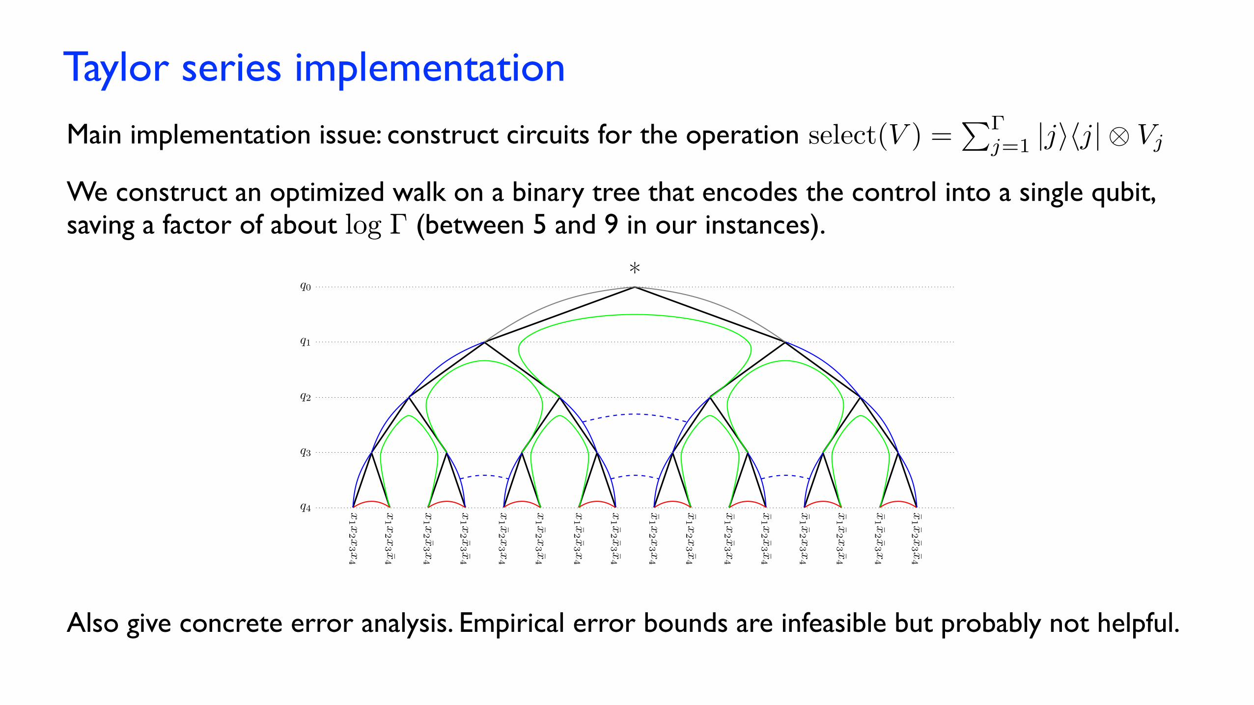
select(V ) =P�

j=1 |jihj|⌦ VjMain implementation issue: construct circuits for the operation

We construct an optimized walk on a binary tree that encodes the control into a single qubit, saving a factor of about log ¡ (between 5 and 9 in our instances).

Quantum signal processing implementation

•Empirical estimate of the error in the Jacobi-Anger expansion saves about 30-45%.•Comprehensive empirical error bounds are just barefly feasible and probably not helpful.

Empirical error bounds:

QSP is built from the same basic subroutines as TS (state preparation, reflection, select(V)).

To compute a sequence of rotation angles that define the algorithm, we must find the roots of a high-degree polynomial to high precision. This can be done in polynomial time (classically), but it’s expensive in practice.

Workarounds:•Compute the gate count using placeholder angles•Consider a segmented version of the algorithm: concatenate segments that are short enough to be simulated. Modest overhead: with M angles, O(n3+4/M) vs. O(n3) for full QSP.

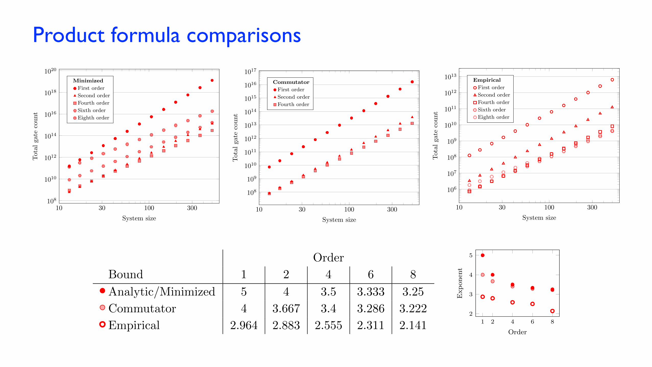
Product formula comparisons

Order

Bound 1 2 4 6 8

Analytic/Minimized 5 4 3.5 3.333 3.25

Commutator 4 3.667 3.4 3.286 3.222

Empirical 2.964 2.883 2.555 2.311 2.1412 4 6 8

2

3

4

5

1

Order

Exponent

10 100108

1010

1012

1014

1016

1018

1020

30 300

System size

Total

gate

count

Minimized

First order

Second order

Fourth order

Sixth order

Eighth order

10 100

108

109

1010

1011

1012

1013

1014

1015

1016

1017

30 300

System size

Total

gate

count

Commutator

First order

Second order

Fourth order

10 100

106

107

108

109

1010

1011

1012

1013

30 300

System size

Total

gate

count

Empirical

First order

Second order

Fourth order

Sixth order

Eighth order

10 100

105

106

107

108

109

1010

20 30 50 70

System size

cnotgate

count

(Cli↵ord+R

z)

PF (com 4)

TS

QSP (seg)

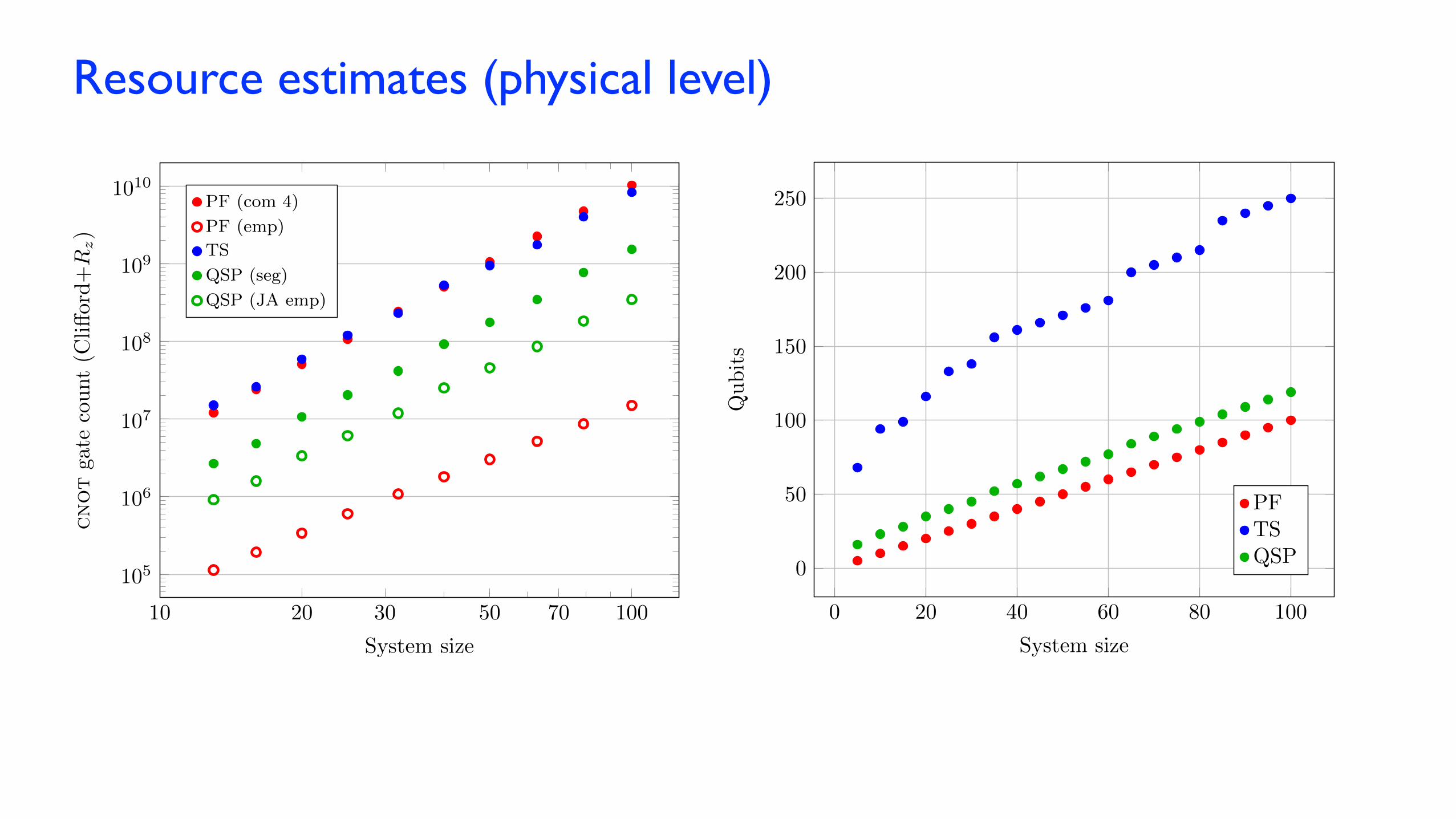
Resource estimates (physical level)

0 20 40 60 80 100

0

50

100

150

200

250

System size

Qubits

PFTSQSP

10 100

105

106

107

108

109

1010

20 30 50 70

System size

cnotgate

count

(Cli↵ord+R

z)

PF (com 4)

PF (emp)

TS

QSP (seg)

QSP (JA emp)

Resource estimates (logical level)

0 20 40 60 80 100

0

50

100

150

200

250

System size

Qubits

PFTSQSP

10 100

107

108

109

1010

1011

1012

20 30 50 70

System size

Tgate

count

(Cli↵ord+T)

PF (com 4)

PF (emp)

TS

QSP (seg)

QSP (JA emp)

Comparisons

Simulating 50 spins (PF6 empirical)•50 qubits•1.8×108 T gates

Factoring a 1024-bit number [Kutin 06]

•3132 qubits•5.7×109 T gates

Simulating FeMoco [Reiher et al. 16]

•111 qubits•1.0×1014 T gates

Simulating 50 spins (segmented QSP)•67 qubits•2.4×109 T gates

10 100 1,000 10,000

108

1010

1012

1014

qubits

Tga

tes

Summary

This work establishes benchmarks for a simple quantum simulation that would be useful and that is classically hard.

More sophisticated algorithms (especially quantum signal processing) are competitive at surprisingly small sizes and give the best approach with rigorous guarantees.

Spin systems are much easier than factoring or quantum chemistry…

… but may still be out of reach of pre-fault tolerant digital quantum computers.

Higher-order product formulas are useful even at very small sizes.

Exisiting analysis of product formulas is very loose.

Outlook

Super-classical quantum simulation without invoking fault tolerance? • Improved error bounds

• Optimized implementations• Alternative target systems• New simulation algorithms• Experiments!

Better provable bounds for simulation algorithms • Product formula error bounds beyond the triangle inequality• Efficient synthesis of the QSP circuit

Resource estimates for more practical models • Architectural constraints, parallelism• Fault-tolerant implementations