PHYSICAL REVIEW RESEARCH 3, 013167 (2021)

Toward pricing financial derivatives with an IBM quantum computer

Ana Martin ,1,* Bruno Candelas ,1,* Ángel Rodríguez-Rozas,2 José D. Martín-Guerrero ,3 Xi Chen,1,4 Lucas Lamata ,5

Román Orús ,6,7,8 Enrique Solano,1,4,7,9 and Mikel Sanz 1,7,9,†

1Department of Physical Chemistry, University of the Basque Country UPV/EHU, Apartado 644, 48080 Bilbao, Spain2Risk Division, Banco Santander, Avenida de Cantabria S/N, 28660 Boadilla del Monte, Madrid, Spain

3IDAL, Electronic Engineering Department, University of Valencia, Avinguda de la Universitat s/n, 46100 Burjassot, Valencia, Spain4International Center of Quantum Artificial Intelligence for Science and Technology (QuArtist) and Physics Department,

Shanghai University, 200444 Shanghai, China5Departamento de Física Atómica, Molecular y Nuclear, Universidad de Sevilla, 41080 Sevilla, Spain6Donostia International Physics Center, Paseo Manuel de Lardizabal 4, 20018 San Sebastián, Spain

7IKERBASQUE, Basque Foundation for Science, Plaza Euskadi 5, 48009 Bilbao, Spain8Multiverse Computing, Pio Baroja 37, 20008 San Sebastián, Spain

9IQM, Nymphenburgerstr. 86, 80636 Munich, Germany

(Received 6 August 2019; revised 1 November 2019; accepted 18 December 2020; published 22 February 2021)

Pricing interest-rate financial derivatives is a major problem in finance, in which it is crucial to accuratelyreproduce the time evolution of interest rates. Several stochastic dynamics have been proposed in the literature tomodel either the instantaneous interest rate or the instantaneous forward rate. A successful approach to model thelatter is the celebrated Heath-Jarrow-Morton framework, in which its dynamics is entirely specified by volatilityfactors. In its multifactor version, this model considers several noisy components to capture at best the dynamicsof several time-maturing forward rates. However, as no general analytical solution is available, there is a trade-offbetween the number of noisy factors considered and the computational time to perform a numerical simulation.Here, we employ the quantum principal component analysis to reduce the number of noisy factors required toaccurately simulate the time evolution of several time-maturing forward rates. The principal components areexperimentally estimated with the five-qubit IBMQX2 quantum computer for 2 × 2 and 3 × 3 cross-correlationmatrices, which are based on historical data for two and three time-maturing forward rates. This paper is astep towards the design of a general quantum algorithm to fully simulate on quantum computers the Heath-Jarrow-Morton model for pricing interest-rate financial derivatives. It shows indeed that practical applications ofquantum computers in finance will be achievable in the near future.

DOI: 10.1103/PhysRevResearch.3.013167

I. INTRODUCTION

In finance, derivatives are contracts whose value derivesfrom the value of an underlying financial asset or a set ofassets, like an index, bonds, currency rates, stocks, marketindices, or interest rates. Typical financial derivatives con-tracts include forwards, futures, swaps (currency swaps orinterest rate swaps), caps, floors, and swaptions, among manyothers. They are typically used either to manage (mitigate)risk exposure (hedging), or for pure speculation. In the caseof pricing interest-rate financial derivatives under the risk-neutral assumption [1,2], it is crucial to model accurately thetime evolution of interest rates. Several stochastic dynamics

*These authors contributed equally to this work.†Corresponding author: mikel.sanz@ehu.es

Published by the American Physical Society under the terms of theCreative Commons Attribution 4.0 International license. Furtherdistribution of this work must maintain attribution to the author(s)and the published article’s title, journal citation, and DOI.

have been proposed in the literature to model either the in-stantaneous interest rate r(t ) (also known as the instantaneousspot rate or, simply, as the short rate) or the instantaneousforward rate, which is the forward rate at a future, infinitesimalperiod (T, T + δt ) forecasted at a previous time t , denotedby f (t, T ) [1]. Simple dynamics based on one or two noisy(random) factors for modeling both the short rate and theforward rates have been proposed [1,3–5]. For short rates,one- and two-factor models became popular, such as the theVasicek model, the Hull-White model, the Cox-Ingesroll-Ross(CIR) model and its CIR++ extension as one-factor models,and the Gaussian-Vasicek model and the Hull-White model,as two-factor models. Furthermore, their corresponding al-gorithms are straightforward to implement. However, thesemodels suffer from the strong requirements which arise fromthe necessity to calibrate to market data and to capture, atthe same time, correlation and covariance structures from thetime evolution of different forward rates. A highly successfulapproach proposed to overcome these constraints is the cele-brated Heath-Jarrow-Morton (HJM) framework [6–9], whichdirectly models the time evolution of forward rates. Indeed,the HJM model is a general family of models from which

2643-1564/2021/3(1)/013167(12) 013167-1 Published by the American Physical Society

ANA MARTIN et al. PHYSICAL REVIEW RESEARCH 3, 013167 (2021)

most of the aforementioned models may be derived [1]. Toget a deeper understanding of this model, we refer the readerto Appendix A. In the HJM model, the dynamics is entirelyspecified by its volatility factors. Although general, there isa trade-off between the number of noisy factors consideredand the computational time when executing the algorithm.Therefore, the computational power limits the accuracy ofthe model. Here is where a quantum computer becomes auseful tool. A quantum computer has a significantly biggercomputational capacity than a classical one; therefore, usingit would allow us to increase the accuracy of the HJM model.

Quantum computing (QC) has emerged in the past yearsas one of the most exciting applications of quantum technolo-gies [10], which promises to revolutionize the computationalpower at our disposal. In QC, entanglement, probably the mostcharacteristic signature of quantum physics, is employed as anextra resource to speed up the performance of the computa-tion, since it allows us to parallelize the calculations. Multiplealgorithms with provable quantum speedup with respect totheir best classical counterparts have been proposed for primefactorization [11], searching in a list [12], solving systemsof linear equations [13], and finding the largest eigenvaluesand eigenvectors of a given matrix [14], among many others.A particularly relevant application is quantum simulation, inwhich a controllable quantum system simulates the dynamicsof another quantum system of interest whose classical simu-lation would be highly inefficient. Examples of applicationsof quantum simulations can be found in spin systems [15,16],quantum chemistry [17–20], quantum field theories [21,22],fluid dynamics [23], and quantum artificial life [24–26]. Someapplications of quantum technologies to finances have alreadybeen proposed [27–31], but only few experiments have beencarried out so far [32–35]. State-of-the-art technology, how-ever, only provides us with small noisy quantum chips, whichlimits the applicability of digital quantum simulations to toymodels.

In this article, we employ an efficient quantum prin-cipal component analysis (qPCA) algorithm to effectivelyreduce the number of noisy factors needed to accurately sim-ulate the joint dynamics of several time-maturing forwardrates, according to the multifactor HJM model. Althoughthis is a general implementation that can be run in anysuperconductive-circuit-based quantum processor, we haveimplemented this algorithm in the five-qubit IBMQX2 su-perconducting quantum processor of IBM due to its easyaccessibility. The volatility factors,

σ̄i(τ j ) =√

λi(vi ) j, (1)

where λi and vi are the eigenvalues and eigenvectors ofthe covariance matrix, respectively, are estimated from 2 × 2and 3 × 3 cross-correlation matrices between different time-maturing forward rates based on historical data. To illustrateour qPCA algorithm, we apply this technique to the covari-ance matrix appearing in Fig. 19.3 in Ref. [36], based onhistorical data for 1-, 3- and 6-month rates:

σ3 =⎛⎝0.000189 0.000097 0.000091

0.000097 0.000106 0.0001010.000091 0.000101 0.000126

⎞⎠. (2)

This is, to our knowledge, both the first quantum comput-ing experiment in financial option pricing and the largestimplementation of the qPCA algorithm on a quantum plat-form. Although for small matrices the problem can be easilysolved on a classical computer, this contribution representsa promising attempt towards the quantum computation oflarge-scale financial problems which are today prohibitivelyexpensive. In the present noisy intermediate-scale quantum(NISQ) technology era [22], we extend the applications ofquantum computers to the field of finance, paving the wayfor achieving useful quantum supremacy or advantage in thefollowing years.

Quantum principal component analysis

Principal component analysis (PCA) is a mathematicaltechnique which allows us to find the optimal low-rank ap-proximation of a given matrix by computing its spectraldecomposition in eigenvalues and eigenvectors. Indeed, thisapproximation discards the smallest eigenvalues of the ma-trix, keeping only the principal components of the spectraldecomposition. This technique is of paramount importance fora variety of applications that go from dimensionality reductionproblems to problems related to finding patterns in data ofbig dimension. Unfortunately, the computational cost is toohigh when the size of the matrix is elevated. It is in thiscontext in which quantum algorithms and quantum computersmay play a relevant role. Indeed, in Ref. [14] the authorsprovided an elegant quantum algorithm to perform PCA withan exponential speedup. The authors assumed that the matrixcan be represented by a quantum state; i.e., it is a non-negativematrix with trace equal to 1, which covers a wide range ofinteresting cases, including the case under study in this paperof covariance matrices associated to volatilities.

In this article, we explore the use of this qPCA techniqueto effectively reduce the dimensionality of the HJM model, byreducing the number of noisy factors without detriment to itsaccuracy. The qPCA algorithm proposed is specially suited forthis financial problem since it is only applicable to density ma-trices, such as the one given by the correlation matrix used asinput for the HJM model. Finally, succeeding in reducing theeffective number of noisy factors turns out to be critical for theconstruction of any quantum Monte Carlo algorithm for thismodel, after reducing the potential number of quantum gatesof the resulting quantum circuit, thus alleviating the limitationin terms of decoherence times of the quantum processor.

We implement a slightly modified version of the aforemen-tioned algorithm, which is better adapted to be run in a smalland noisy quantum chip, typical in this NISQ technology era[37]. This allows us to reduce the number of noisy factorspresented within the HJM model. This is the first step towardthe construction of a general quantum computing algorithm tofully simulate the HJM model on the IBM quantum computerfor pricing interest-rate financial derivatives. In the followingsection, we briefly describe the algorithm.

II. QUANTUM CIRCUIT

Let us consider a non-negative matrix σN ∈ RN × RN withtr[σN ] = 1, which is the matrix whose principal componentswe want to compute. Let us assume that we can efficiently

013167-2

TOWARD PRICING FINANCIAL DERIVATIVES WITH AN … PHYSICAL REVIEW RESEARCH 3, 013167 (2021)

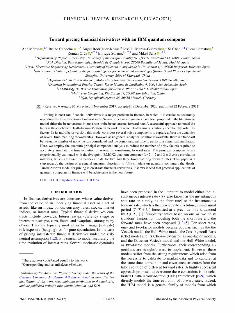
FIG. 1. Quantum circuit implementation for n + log N qubits. The first n qubits are dedicated to the binary codification of the maximumeigenvalue of the matrix σN and they are initialized in the site |0〉. The rest of the qubits, a total of log N , encode the estimation of thecorresponding eigenvector and are initialized on a random state |b〉. The single qubit gate H corresponds to the Hadamard gate. The rest of thegates are controlled operations. The controlled U 2k

ρ gate applies the matrix U = eitσN 2k times on the last set of qubits. The controlled R†k gate

applies the matrix (1 00 e2π i/2k ) to each target qubit. After performing all the operations, if the initial |b〉 is appropriate, one gets the final state

|b1b2 · · · bn〉 ⊗ |umax〉, where |b1b2 · · · bn〉 is the n-bit estimation of the eigenvalue λ(n)j and |umax〉 is the best estimation of the exact eigenvector

of σN .

generate the unitary eitσN . It has been proven in the literaturethat, under certain conditions such as sparsity of the matrix[38,39] or access to several copies of σN [14], this is possible.In our case the covariance matrix σN is not sparse, but wecan access several copies of it codified in quantum states.Thus, the best way to efficiently generate the unitary operationeitσN with accuracy ε in O(t2ε−1) steps is the one describedby Lloyd et al in Ref. [14]. This matrix admits a spectraldecomposition σN = ∑N

j=1 λ j |u j〉〈u j |, with 0 � λ j � 1 and∑Nj=1 λ j = 1, and we assume that σN can be very well approx-

imated by a matrix ρr = ∑rj=1 λ j |u j〉〈u j | with rank r � N .

Therefore, the goal of the algorithm is the determination ofthe r largest eigenvalues of σN and their corresponding eigen-vectors. If we want to determine the eigenvalues with an n-bitprecision, we will need n + log N qubits, as depicted in Fig. 1,which represents the gate decomposition of the algorithm. Apriori, we do not know the eigenvectors of our algorithm.Hence, we cannot make use of quantum phase estimation tocompute directly the corresponding eigenvalue. Consequently,we initialize our system in a random state |b〉 whose (un-known) decomposition in terms of the eigenbasis is given by|b〉 = ∑N

j=1 β j |u j〉. If we take a random vector, the probabilitythat there exists a component βk = 0 is zero. The quantumstate after the quantum Fourier transform can be written as|b〉 = ∑N

j=1 β j |�(n)j 〉 ⊗ |u j〉, so eigenvalues and eigenvec-

tors are entangled. �(n)j = 0.b1b2 · · · bn is the n-bit precision

binary representation of the jth eigenvalue of ρr . However,if our assumption that σN is well approximated by the r-rankmatrix ρr is correct, then the highest eigenvalues should bearound 1/r ≈ ∑n

k=1 yk2−k . Calling |y(n)〉 = |y1 y2 · · · yn〉 thevector of these components, it means that, by projecting theeigenvalue component |�(n)

j 〉 of the state |b〉 around thiscomponent, one may obtain the eigenvector corresponding tothe maximum eigenvalue, i.e., 〈y(n)| ⊗ 1|b〉 ≈ |umax〉. It ispossible, especially when n is small, as may happen in theNISQ chips, that the n-bit approximation of the eigenvaluecannot be able to distinguish between two or more eigen-vectors. In this case, the projection is not into the maximumeigenvalue, but into a K-dimensional subspace containing the

indistinguishable components 〈y(n)| ⊗ 1|b〉 = ∑Kj=1 β̃ j |u j〉,

where the β̃ j are the normalized β j in the subspace. As wedo not know a priori whether K > 1 or not, we could startwith a different random state |c〉 = ∑N

j=1 γ j |u j〉, which leads

to |c〉 = ∑Nj=1 γ j |�(n)

j 〉 ⊗ |u j〉. After projecting into |y(n)〉the expected state is a different superposition

∑Lj=1 γ̃ j |u j〉

with high probability, which helps us to check whether wehave actually identified the eigenvector corresponding to themaximum eigenvalue. Otherwise, we must increase the n-bitprecision until a unique eigenvalue is identified.

Let us assume now that the n-bit precision is sufficientto determine a unique eigenvector. Taking into account theconstraints due to the small number of qubits and the noiseof the chip and the operations, we can sequentially improvethe result of the eigenvector. As described above, we start theprotocol with a random quantum state |b0〉, to which the noisyalgorithm is applied and the projection into the |y(n)〉 subspaceis performed. Let us call the result |b0〉, which is an approx-imation for the eigenvector. If we employ now this state asthe initial state in the protocol, |b0〉 = |b1〉, then one expectsthat the approximation for the eigenvector provided by |b1〉improves the fidelity due to the cancellation of coherent errorsassociated to the β components. Nonetheless, there is a limita-tion in this sequential improvement related to the decoherenceof the qubits and the statistical error of the measurement.In any case, the result can be (slightly) further improved byperforming measurements in different bases and averaging,since this cancels some systematic errors of the gates.

III. RESULTS

As described in the previous section, the protocol is di-vided into two parts. First, we estimate the eigenvector |umax〉corresponding to the largest eigenvalue λmax. We start witha random state, apply the circuit implementation shown inFig. 2, project on the binary n-bit estimation for the largesteigenvalue |y(n)〉, and use this state as the initial state of theprocess, which sequentially approaches the exact eigenvector.Afterwards, we use this eigenvector to get a more accurate

013167-3

ANA MARTIN et al. PHYSICAL REVIEW RESEARCH 3, 013167 (2021)

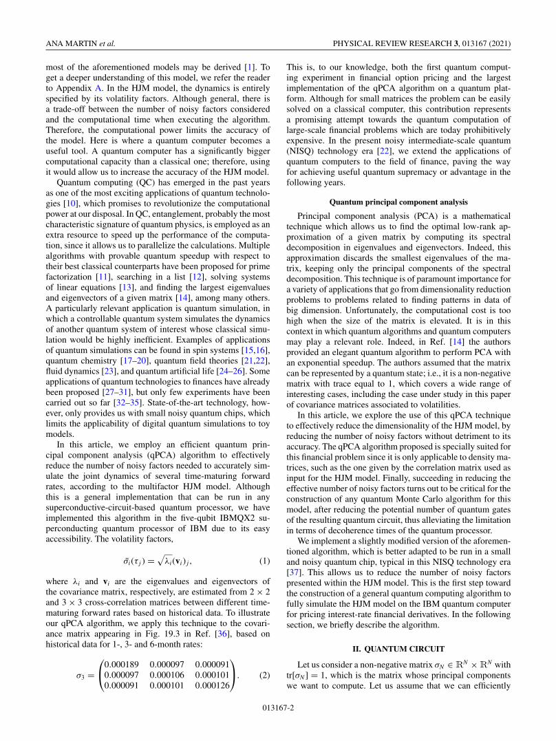
FIG. 2. (a) Quantum circuit implementation for the 2 × 2 ma-trix. The first two qubits encode the 2-bit estimation of the greatesteigenvalue of ρ2 and are initialized on the state |0〉. The last qubitis dedicated to the estimation of the corresponding eigenvector. It isinitialized on a random state |b〉. For the first iteration, we initialize iton the state |+〉 by applying a Hadamard gate. The single-qubit gatesrepresented by the letter H refer to the Hadamard gate. The con-trolled U gates represent the unitary controlled operations called U 2k

ρ

in Fig. 1. The last two-qubit gate is a controlled S† gate, controllingthe first qubit and acting on the second. The final state of the systemafter running the circuit and taking measures is |11〉 ⊗ (0.719|0〉 +0.659|1〉). (b) Populations for each iteration. The graphic shows theexperimental probabilities of finding the three qubits in each state andits corresponding errors for the four iterations of the algorithm. Wehave considered both statistical and experimental errors, assumingfor the latter an error of 8% for each two-qubit gate.

approximation for the eigenvalue λmax by means of quantumphase estimation.

For the estimation of the eigenvector, we start with arandom state |b0〉. Hence, the initial state of the system is|0〉 ⊗ |0〉 ⊗ |b0〉. After the first iteration and projecting on thecomputational basis the eigenvector, we obtain a first esti-mation, which we call |b1〉, and use it as the initial state ofthe system on the next iteration. This is |0〉 ⊗ |0〉 ⊗ |b1〉. Wecontinue this process and iterate k times until |bk−1〉 ≈ |bk〉.Once we reach that point, we can say that |bk〉 ≈ |umax〉.

Let us now estimate the eigenvalue λmax. Once the first partis finished and we have an accurate approximation for |umax〉,we can apply quantum phase estimation [10] to obtain λmax

with n-bit precision. The precision is limited in this case bythe size of the processor. Our aim is to apply the algorithm tothe 3 × 3 matrix given in Eq. (2) in the five-qubit IBMQX2quantum processor. First, we solve the 2 × 2 submatrix ofσ3 containing only two maturities, and afterwards, we solvethe 4 × 4 expansion of the same matrix. Despite the smallsize of the problem, the volume of the quantum algorithmsallowed in this processor is almost achieved, but we can stillobtain relatively accurate results. We have run the algorithm inboth the simulator provided by QISKIT [40] and the real IBMquantum processor, reaching accurate results in both cases.

A. 2 × 2 matrix

First, we need to codify the covariance matrix in a quantumstate, so we only need to normalize it with respect to its trace,

ρ2 = σ2

tr(σ2)=

(0.6407 0.32880.3288 0.3593

), (3)

whose spectral decomposition is given by

λ1 = 0.8576, |u1〉 = 0.8347|0〉 + 0.5508|1〉, (4)

λ2 = 0.1424, |u2〉 = 0.5508|0〉 − 0.8347|1〉. (5)

Let us remark that λmax � λ2, a usual characteristic of thesecorrelation matrices, so we can apply the PCA technique tofind the optimal low-rank approximation of ρ2. Let us nowdefine the unitary

Uρ2 = e2π iρ2 =(

0.6260 − 0.3068i −0.7170i−0.7170i 0.6260 + 0.3068i

).

(6)For the first part of the protocol, we make use of three

qubits, two for a 2-bit approximation of the eigenvalue, anda third one one to represent the eigenvector. We apply thefirst part of the protocol as described above, starting with aquantum state |b0〉 = 1√

2(|0〉 + |1〉) and projecting into the

|y(n)〉 = |11〉 state. After the fourth iteration, each of them av-eraged over 8192 realizations, the outcome vector estimatingthe eigenvector stabilizes and we stop. With this final eigen-vector, we also rotate the measurement basis in x, y, and anarbitrary direction r = (cos α,−eiβ sin α; eiβ sin α, eiγ cos α)to compute the relative phase and to improve the accuracy ofthe solution provided. We have chosen the set of angles α =1.00, β = 0.80, and γ = 0.16, but any other choice would bevalid as long as all of the angles are different from zero. Ourestimation for |umax〉 is consequently given by

|umax〉 = [(0.87 ± δ) − i(0.10 ± δ)]|0〉+[(0.47 ± δ) + i(0.10 ± δ)]|1〉, (7)

with δ = 0.9 the error estimated from the two-qubit gatesand measurement fidelity provided by IBM and the statisticalerror related to the number of repetitions. This δ should beunderstood as an upper bound of all possible errors, includ-ing not only the gate and qubit errors provided by IBMQ,but also other errors, which do not increase with the depthof the algorithm, such as T1 and T2, measurement errors,crosstalk, non-Markovian errors, etc. As we had no directaccess to the processor, it is not possible to distinguish amongthem, so we consider the worst possible case. In AppendixB we provide more information about how we have esti-mated the error δ. Let us remark that we have split thecomplex phase between both states using the global phase.The estimation for the coefficients after each iteration in thez basis is provided in Table I. We can observe that the al-gorithm has already converged in the first iteration, and thevariations are within the estimated error. We take the eigen-vector produced in the last iteration and repeat the algorithmwith this one as the initial state measuring in x, y, and r-random directions to check possible relative phases and to tryto remove systematic errors, which yields the states |bx〉 =

013167-4

TOWARD PRICING FINANCIAL DERIVATIVES WITH AN … PHYSICAL REVIEW RESEARCH 3, 013167 (2021)

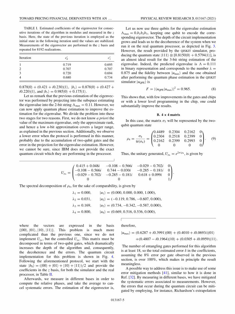
TABLE I. Estimated coefficients of the eigenvector for consec-utive iterations of the algorithm in modulus and measured in the zbasis. Here, the state of the previous iteration is employed as theinitial state in the following iteration until the values are stabilized.Measurements of the eigenvector are performed in the z basis andrepeated for 8192 realizations.

Iteration cz0 cz

1

1 0.719 0.6952 0.707 0.7073 0.720 0.6944 0.680 0.734

0.878|0〉 + (0.421 + i0.230)|1〉, |by〉 = 0.878|0〉 + (0.427 +i0.220)|1〉, and |br〉 = 0.985|0〉 + 0.175|1〉.

Let us remark that the previous estimation of the eigenvec-tor was performed by projecting into the subspace estimatingthe eigenvalue into the 2-bit string �max = 0.11. However, wecan now apply quantum phase estimation to improve the es-timation for the eigenvalue. We divide the problem into thesetwo stages for two reasons. First, we do not know a priori thevalue of the maximum eigenvalue, only the approximate rank,and hence a low n-bit approximation covers a larger range,as explained in the previous section. Additionally, we observea lower error when the protocol is performed in this manner,probably due to the accumulation of two-qubit gates and theerror in the projection for the eigenvalue estimation. However,we cannot be sure, since IBM does not provide the exactquantum circuit which they are performing in the processor.

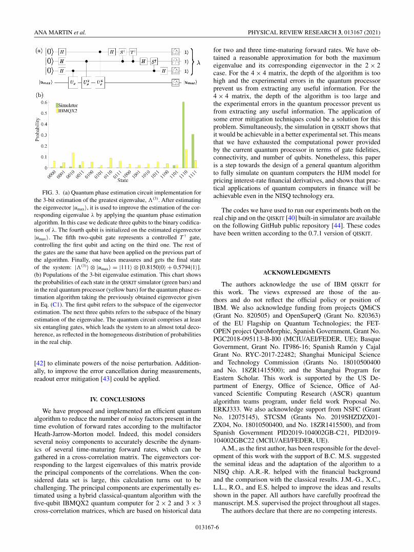
Let us now use three qubits for the eigenvalue estimation�max = 0.b1b2b3, keeping one qubit to encode the corre-sponding eigenvector. The depth of the circuit implementationgrows and leads us to the decoherence of the system when werun it on the real quantum processor, as depicted in Fig. 3.However, the result provided by the QISKIT simulator, pro-ducing the quantum state |111〉 ⊗ [0.8150|0〉 + 0.5794|1〉], isan almost ideal result for the 3-bit string estimation of theeigenvalue. Indeed, the predicted eigenvalue is � = 0.111in binary representation and corresponds to the number λ =0.875 and the fidelity between |umax〉 and the one obtainedafter performing the quantum phase estimation in the QISKIT

simulator |uQPE〉 is

F = |〈uQPE|umax〉|2 = 0.965. (8)

This shows that, with few improvements in the gates and chipsor with a lower level programming in the chip, one couldsubstantially improve the results.

B. 4 × 4 matrix

In this case, the matrix σ3 will be represented by the two-qubit quantum state

ρ4 = σ4

tr(σ4)=

⎛⎜⎝

0.4489 0.2304 0.2162 00.2304 0.2518 0.2399 00.2162 0.2399 0.2993 0

0 0 0 0

⎞⎟⎠. (9)

Thus, the unitary generated, Uρ4 = e2π iρ4 , is given by

Uρ4 =

⎛⎜⎝

0.415 + 0.048i −0.108 − 0.566i −0.029 − 0.702i 0−0.108 − 0.566i 0.744 − 0.030i −0.285 − 0.181i 0−0.029 − 0.702i −0.285 − 0.181i 0.618 + 0.099i 0

0 0 0 1

⎞⎟⎠.

The spectral decomposition of ρ4, for the sake of comparability, is given by

λ1 = 0.000, |u1〉 = (0.000, 0.000, 0.000, 1.000),

λ2 = 0.031, |u2〉 = (−0.119, 0.786,−0.607, 0.000),

λ3 = 0.169, |u3〉 = (0.734,−0.342,−0.587, 0.000),

λ4 = 0.800, |u4〉 = (0.669, 0.516, 0.536, 0.000),

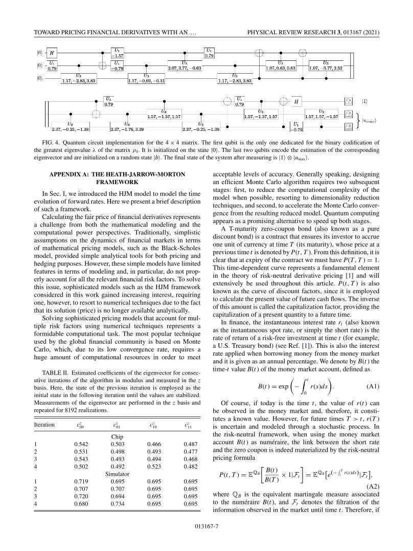
where the vectors are expressed in the basis{|00〉, |01〉, |10〉, |11〉}. This problem is much morecomplicated than the previous one, since we do notimplement Uρ4 , but the controlled Uρ4 . This matrix must bedecomposed in terms of two-qubit gates, which dramaticallyincreases the depth of the algorithm and, consequently,the decoherence and the errors. The quantum circuitimplementation for this problem is shown in Fig. 4.Following the aforementioned protocol, we start with thestate |b0〉 = (|00〉 + |01〉 + |10〉 + |11〉)/2 and provide thecoefficients in the z basis, for both the simulator and the realprocessor, in Table II.

Afterwards, we measure in different bases in order tocompute the relative phases, and take the average to can-cel systematic errors. The estimation of the eigenvector is,

therefore,

|umax〉 = (0.6287 + i0.3991)|00〉 + (0.4010 + i0.0693i)|01〉+(0.4807 − i0.1964)|10〉 + (0.0305 + i0.0959)|11〉.

The number of entangling gates performed for this algorithmis at least 18, so the total estimated error δ in the coefficients,assuming the 8% error per gate observed in the previoussection, is over 100%, which makes in principle the resultmeaningless.

A possible way to address this issue is to make use of someerror mitigation methods [41], similar to how it is done inRef. [32]. By measuring in different bases, we have mitigatedthe systematic errors associated to measurements. However,the errors that occur during the quantum circuit can be miti-gated by employing, for instance, Richardson’s extrapolation

013167-5

ANA MARTIN et al. PHYSICAL REVIEW RESEARCH 3, 013167 (2021)

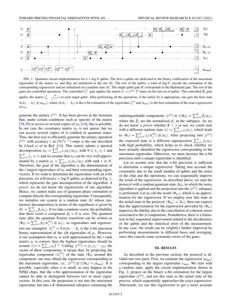
FIG. 3. (a) Quantum phase estimation circuit implementation forthe 3-bit estimation of the greatest eigenvalue, �(3). After estimatingthe eigenvector |umax〉, it is used to improve the estimation of the cor-responding eigenvalue λ by applying the quantum phase estimationalgorithm. In this case we dedicate three qubits to the binary codifica-tion of λ. The fourth qubit is initialized on the estimated eigenvector|umax〉. The fifth two-qubit gate represents a controlled T † gate,controlling the first qubit and acting on the third one. The rest ofthe gates are the same that have been applied on the previous part ofthe algorithm. Finally, one takes measures and gets the final stateof the system: |�(3)〉 ⊗ |umax〉 = |111〉 ⊗ [0.8150|0〉 + 0.5794|1〉].(b) Populations of the 3-bit eigenvalue estimation. This chart showsthe probabilities of each state in the QISKIT simulator (green bars) andin the real quantum processor (yellow bars) for the quantum phase es-timation algorithm taking the previously obtained eigenvector givenin Eq. (C1). The first qubit refers to the subspace of the eigenvectorestimation. The next three qubits refers to the subspace of the binaryestimation of the eigenvalue. The quantum circuit comprises at leastsix entangling gates, which leads the system to an almost total deco-herence, as reflected in the homogeneous distribution of probabilitiesin the real chip.

[42] to eliminate powers of the noise perturbation. Addition-ally, to improve the error cancellation during measurements,readout error mitigation [43] could be applied.

IV. CONCLUSIONS

We have proposed and implemented an efficient quantumalgorithm to reduce the number of noisy factors present in thetime evolution of forward rates according to the multifactorHeath-Jarrow-Morton model. Indeed, this model considersseveral noisy components to accurately describe the dynam-ics of several time-maturing forward rates, which can begathered in a cross-correlation matrix. The eigenvectors cor-responding to the largest eigenvalues of this matrix providethe principal components of the correlations. When the con-sidered data set is large, this calculation turns out to bechallenging. The principal components are experimentally es-timated using a hybrid classical-quantum algorithm with thefive-qubit IBMQX2 quantum computer for 2 × 2 and 3 × 3cross-correlation matrices, which are based on historical data

for two and three time-maturing forward rates. We have ob-tained a reasonable approximation for both the maximumeigenvalue and its corresponding eigenvector in the 2 × 2case. For the 4 × 4 matrix, the depth of the algorithm is toohigh and the experimental errors in the quantum processorprevent us from extracting any useful information. For the4 × 4 matrix, the depth of the algorithm is too large andthe experimental errors in the quantum processor prevent usfrom extracting any useful information. The application ofsome error mitigation techniques could be a solution for thisproblem. Simultaneously, the simulation in QISKIT shows thatit would be achievable in a better experimental set. This meansthat we have exhausted the computational power providedby the current quantum processor in terms of gate fidelities,connectivity, and number of qubits. Nonetheless, this paperis a step towards the design of a general quantum algorithmto fully simulate on quantum computers the HJM model forpricing interest-rate financial derivatives, and shows that prac-tical applications of quantum computers in finance will beachievable even in the NISQ technology era.

The codes we have used to run our experiments both on thereal chip and on the QISKIT [40] built-in simulator are availableon the following GitHub public repository [44]. These codeshave been written according to the 0.7.1 version of QISKIT.

ACKNOWLEDGMENTS

The authors acknowledge the use of IBM QISKIT forthis work. The views expressed are those of the au-thors and do not reflect the official policy or position ofIBM. We also acknowledge funding from projects QMiCS(Grant No. 820505) and OpenSuperQ (Grant No. 820363)of the EU Flagship on Quantum Technologies; the FET-OPEN project QuroMorphic, Spanish Government, Grant No.PGC2018-095113-B-I00 (MCIU/AEI/FEDER, UE); BasqueGovernment, Grant No. IT986-16; Spanish Ramón y CajalGrant No. RYC-2017-22482; Shanghai Municipal Scienceand Technology Commission (Grants No. 18010500400and No. 18ZR1415500); and the Shanghai Program forEastern Scholar. This work is supported by the US De-partment of Energy, Office of Science, Office of Ad-vanced Scientific Computing Research (ASCR) quantumalgorithm teams program, under field work Proposal No.ERKJ333. We also acknowledge support from NSFC (GrantNo. 12075145), STCSM (Grants No. 2019SHZDZX01-ZX04, No. 18010500400, and No. 18ZR1415500), and fromSpanish Government PID2019-104002GB-C21, PID2019-104002GBC22 (MCIU/AEI/FEDER, UE).

A.M., as the first author, has been responsible for the devel-opment of this work with the support of B.C. M.S. suggestedthe seminal ideas and the adaptation of the algorithm to aNISQ chip. A.R.-R. helped with the financial backgroundand the comparison with the classical results. J.M.-G., X.C.,L.L., R.O., and E.S. helped to improve the ideas and resultsshown in the paper. All authors have carefully proofread themanuscript. M.S. supervised the project throughout all stages.

The authors declare that there are no competing interests.

013167-6

TOWARD PRICING FINANCIAL DERIVATIVES WITH AN … PHYSICAL REVIEW RESEARCH 3, 013167 (2021)

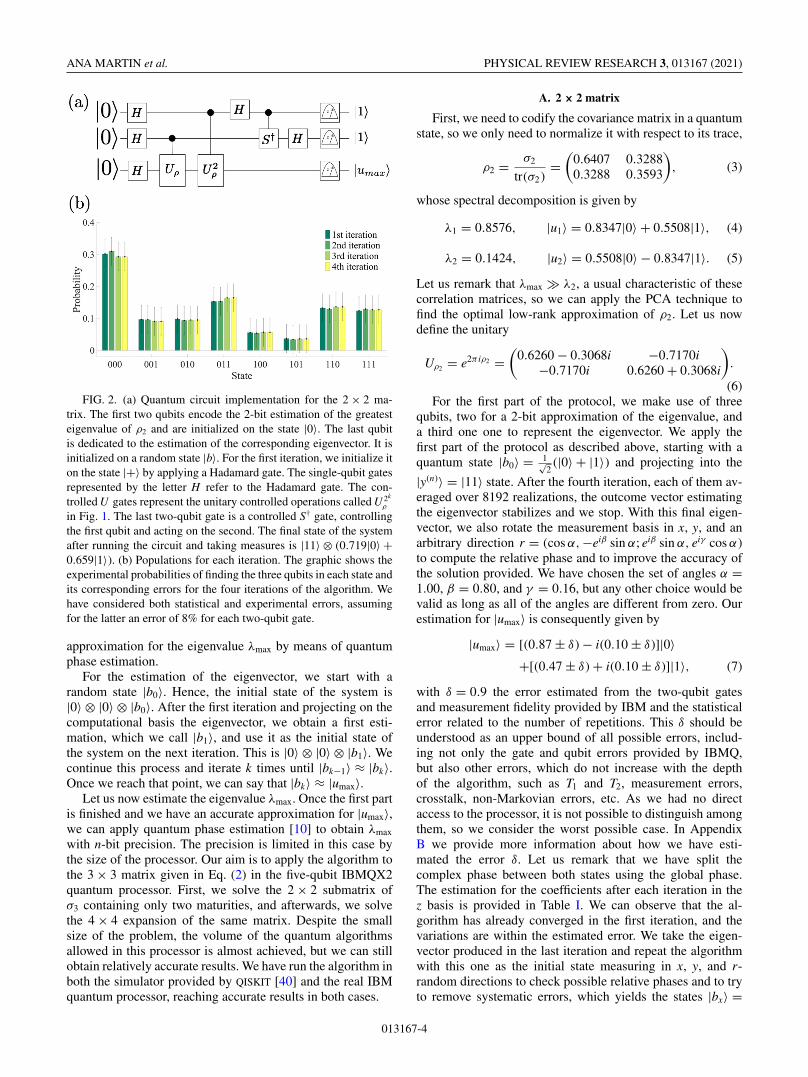
FIG. 4. Quantum circuit implementation for the 4 × 4 matrix. The first qubit is the only one dedicated for the binary codification ofthe greatest eigenvalue λ of the matrix ρ4. It is initialized on the state |0〉. The last two qubits encode the estimation of the correspondingeigenvector and are initialized on a random state |b〉. The final state of the system after measuring is |1〉 ⊗ |umax〉.

APPENDIX A: THE HEATH-JARROW-MORTONFRAMEWORK

In Sec. I, we introduced the HJM model to model the timeevolution of forward rates. Here we present a brief descriptionof such a framework.

Calculating the fair price of financial derivatives representsa challenge from both the mathematical modeling and thecomputational power perspectives. Traditionally, simplisticassumptions on the dynamics of financial markets in termsof mathematical pricing models, such as the Black-Scholesmodel, provided simple analytical tools for both pricing andhedging purposes. However, these simple models have limitedfeatures in terms of modeling and, in particular, do not prop-erly account for all the relevant financial risk factors. To solvethis issue, sophisticated models such as the HJM frameworkconsidered in this work gained increasing interest, requiringone, however, to resort to numerical techniques due to the factthat its solution (price) is no longer available analytically.

Solving sophisticated pricing models that account for mul-tiple risk factors using numerical techniques represents aformidable computational task. The most popular techniqueused by the global financial community is based on MonteCarlo, which, due to its low convergence rate, requires ahuge amount of computational resources in order to meet

TABLE II. Estimated coefficients of the eigenvector for consec-utive iterations of the algorithm in modulus and measured in the zbasis. Here, the state of the previous iteration is employed as theinitial state in the following iteration until the values are stabilized.Measurements of the eigenvector are performed in the z basis andrepeated for 8192 realizations.

Iteration cz00 cz

01 cz10 cz

11

Chip1 0.542 0.503 0.466 0.4872 0.531 0.498 0.493 0.4773 0.543 0.493 0.494 0.4684 0.502 0.492 0.523 0.482

Simulator1 0.719 0.695 0.695 0.6952 0.707 0.707 0.695 0.6953 0.720 0.694 0.695 0.6954 0.680 0.734 0.695 0.695

acceptable levels of accuracy. Generally speaking, designingan efficient Monte Carlo algorithm requires two subsequentstages: first, to reduce the computational complexity of themodel when possible, resorting to dimensionality reductiontechniques, and second, to accelerate the Monte Carlo conver-gence from the resulting reduced model. Quantum computingappears as a promising alternative to speed up both stages.

A T-maturity zero-coupon bond (also known as a purediscount bond) is a contract that ensures its investor to accrueone unit of currency at time T (its maturity), whose price at aprevious time t is denoted by P(t, T ). From this definition, it isclear that at expiry of the contract we must have P(T, T ) = 1.This time-dependent curve represents a fundamental elementin the theory of risk-neutral derivative pricing [1] and willextensively be used throughout this article. P(t, T ) is alsoknown as the curve of discount factors, since it is employedto calculate the present value of future cash flows. The inverseof this amount is called the capitalization factor, providing thecapitalization of a present quantity to a future time.

In finance, the instantaneous interest rate rt (also knownas the instantaneous spot rate, or simply the short rate) is therate of return of a risk-free investment at time t (for example,a U.S. Treasury bond) (see Ref. [1]). This is also the interestrate applied when borrowing money from the money marketand it is given as an annual percentage. We denote by B(t ) thetime-t value B(t ) of the money market account, defined as

B(t ) = exp

(−

∫ t

0r(s)ds

). (A1)

Of course, if today is the time t , the value of r(t ) canbe observed in the money market and, therefore, it consti-tutes a known value. However, for future times T > t , r(T )is uncertain and modeled through a stochastic process. Inthe risk-neutral framework, when using the money marketaccount B(t ) as numéraire, the link between the short rateand the zero coupon is indeed materialized by the risk-neutralpricing formula

P(t, T ) = EQB

[B(t )

B(T )× 1|Ft

]= EQB

[e(−

∫ Tt r(s)ds)|Ft

],

(A2)where QB is the equivalent martingale measure associatedto the numéraire B(t ), and Ft denotes the filtration of theinformation observed in the market until time t . Therefore, if

013167-7

ANA MARTIN et al. PHYSICAL REVIEW RESEARCH 3, 013167 (2021)

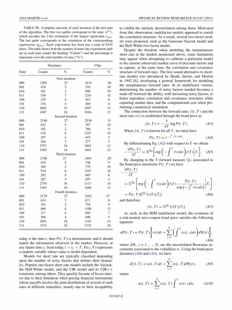
TABLE III. Complete outcome of each iteration of the first partof the algorithm. The first two qubits correspond to the state |λ(n)〉,which encodes the 2-bit estimation of the largest eigenvalue λmax.The last qubit corresponds to the estimation of the correspondingeigenvector |umax〉. Each experiment has been run a total of 8192times. The table shows both the number of times the experiment endsup on each state (under the heading “Counts”) and the percentage itrepresents over the total number of runs (“%”).

Simulator Chip

State Counts % Counts %

First iteration000 2205 27 2474 30001 428 5 793 10010 181 2 808 10011 558 7 1253 15100 325 4 457 6101 316 4 304 4110 2692 33 1087 13111 1487 18 1016 12

Second iteration000 2190 27 2538 31001 422 5 787 10010 181 2 766 9011 516 6 1257 15100 297 4 443 5101 264 3 277 3110 2757 34 1063 13111 1565 19 1061 13

Third iteration000 2196 27 2401 29001 418 5 746 9010 169 2 779 10011 510 6 1347 16100 292 4 465 6101 287 4 297 4110 2755 34 1117 14111 1565 19 1040 13

Fourth iteration000 2179 27 2182 27001 414 5 671 8010 191 2 754 9011 469 6 1100 13100 317 4 605 7101 306 4 400 5110 2801 34 1145 14111 1515 18 1335 16

today is the time t , then P(t, T ) is deterministic and it shouldmatch the information observed in the market. However, atany future time t f from today, t < t f < T , P(t f , T ) representsa random variable whose value is model dependent.

Models for short rate are typically classified dependingupon the number of noisy factors that defines their dynam-ics. Popular one-factor short-rate models include the Vasicek,the Hull-White model, and the CIR model and its CIR++extension, among others. They quickly became of lesser inter-est due to their limitation when pricing financial instrumentswhose payoffs involve the joint distribution of several of suchrates at different maturities, mainly due to their incapability

to exhibit the intrinsic decorrelation among them. Motivatedfrom this observation, multifactor models appeared to enrichthe correlation structure. As a result, several two-factor mod-els were proposed, such as the Gaussian-Vasicek model andthe Hull-White two-factor model.

Despite the freedom when modeling the instantaneousshort rate in the models mentioned above, some limitationsmay appear when attempting to calibrate a particular modelto the current (observed) market curve of discount factors andto capture, at the same time, the correlation and covariancestructure of forward rates. The first sound alternative to short-rate models was introduced by Heath, Jarrow, and Mortonin 1992 [8], developing a general framework for modelingthe instantaneous forward rates. In its multifactor version,determining the number of noisy factors needed becomes atrade-off between the ability, with increasing noisy factors, tobetter reproduce correlation and covariance structures whilecapturing market data, and the computational cost when per-forming a numerical simulation.

The connection between the forward rates f (t, T ) and theshort rate r(t ) is established through the bond price as

f (t, T ) = − ∂

∂Tlog P(t, T ). (A3)

When f (t, T ) is known for all T , we must have

P(t, T ) = e− ∫ Tt f (t,s)ds. (A4)

By differentiating Eq. (A2) with respect to T we obtain

−∂P(t, T )

∂T= EQB

[exp

(−

∫ T

tr(s)ds

)r(T )

∣∣∣∣Ft

]. (A5)

By changing to the T -forward measure QT associated tothe bond price numéraire P(t, T ) we have

−∂P(t, T )

∂T

= EQT

[exp

(−

∫ T

tr(s)ds

)r(T )

P(t, T )

exp(− ∫ T

t r(s)ds)∣∣∣∣∣Ft

]

= P(t, T )EQT [r(T )|Ft ], (A6)

and therefore,

f (t, T ) = EQT [r(T )|Ft ]. (A7)

As such, in the HJM multifactor model, the evolution ofa risk-neutral zero-coupon bond price satisfies the followingequation:

dP(t, T ) = P(t, T )

{r(t )dt +

N∑i=1

(∫ T

tσi(t, s)ds

)dWi(t )

},

(A8)where dWi, i = 1, . . . , N , are the uncorrelated Brownian in-crements associated to the volatilities σi. Using the bond pricedynamics (A8) and (A3), we have

df (t, T ) = α(t, T )dt +N∑

i=1

σi(t, T )dWi(t ), (A9)

where

α(t, T ) =N∑

i=1

σi(t, T )∫ T

tσi(t, s)ds. (A10)

013167-8

TOWARD PRICING FINANCIAL DERIVATIVES WITH AN … PHYSICAL REVIEW RESEARCH 3, 013167 (2021)

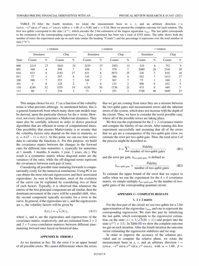
TABLE IV. After the fourth iteration, we rotate the measurement basis in x, y, and an arbitrary direction r =(cos α, −eiβ sin α; eiβ sin α, eiγ cos α), with α = 1.00, β = 0.80, and γ = 0.16. Here we present the complete outcome for each rotation. Thefirst two qubits correspond to the state |�(n)〉, which encodes the 2-bit estimation of the largest eigenvalue λmax. The last qubit correspondsto the estimation of the corresponding eigenvector |umax〉. Each experiment has been run a total of 8192 times. The table shows both thenumber of times the experiment ends up on each state (under the heading “Counts”) and the percentage it represents over the total number ofruns (“%”).

x rotation y rotation r rotation

Simulator Chip Simulator Chip Simulator Chip

State Counts % Counts % Counts % Counts % Counts % Counts %

000 2215 27 2642 32 2229 27 2503 31 519 6 752 9001 340 4 599 7 436 5 570 7 2089 26 2341 29010 633 8 2183 27 631 8 2072 25 236 3 810 10011 77 1 297 4 145 2 360 4 542 7 1413 17100 588 7 557 7 549 7 567 7 75 1 160 2101 4 0 125 2 3 0 133 2 508 6 422 5110 4249 52 1555 19 4126 50 1736 21 475 6 449 5111 86 1 234 3 73 1 251 3 3748 46 1845 23

This unique choice for α(t, T ) as a function of the volatilityterms is what prevents arbitrage. As mentioned before, this isa general framework from which many short-rate models maybe derived, upon the particular choices for the σ terms. How-ever, not every choice generates a Markovian dynamics. Theymust also be carefully selected in order to derive practicalalgorithms that are efficient in terms of computational times.One possibility that ensures Markovianity is to assume thatthe volatility factors only depend on the time to maturity, soσi = σ̄i(T − t ) = σ̄i(τ ). At this point, we can use time seriesdata to calculate the functions σ̄i. For this purpose, we buildthe covariance matrix between the changes in the forwardrates for different time maturities τ j (typically for maturitiesat 1 month, 3 months, 6 monts, 1 year, 2 years, etc.). Theresult is a symmetric matrix whose diagonal terms are thevariances of the rates, while the off-diagonal terms representthe covariances between each pair of rates.

Considering all possible time-maturing forwards is compu-tationally costly for the numerical simulations. Using PCA wecan obtain the most relevant eigenvectors and their associatedeigenvalues. As seen in the literature, most of the evolutionof the curve can be explained by considering two or threeof such factors. Typically, it is observed that whenever theentries of the first principal component are all similar, then thedominant movement of the curve will be a parallel shift. Also,the second component typically accounts for a twist in thecurve. In general, if the eigenvalues are λi and the eigenvectorsare vi, the volatility factors will be given by

σ̄i(τ j ) =√

λi(vi ) j . (A11)

where λi and vi are the eigenvalues and eigenvectors of thecovariance matrix, respectively, and are estimated from 2 × 2and 3 × 3 cross-correlation matrices between different time-maturing forward rates based on historical data.

APPENDIX B: ERROR δ

As we mention in Sec. III, the error δ is an upper boundof all possible errors. We cannot differentiate where the errors

that we get are coming from since they are a mixture betweenthe two-qubit gates and measurement errors and the inherenterrors of the system, which does not increase with the depth ofthe circuit. Thus, we have to consider the worst possible case,where all of the possible errors are taking place.

We first run the experiment for the 2 × 2 covariance matrixand compute the fidelity of our circuit. After running this firstexperiment successfully and assuming that all of the errorsthat we get are a consequence of the two-qubit gate error, weestimate the error per two-qubit gate. Thus, the total error δ ofthe process might be described as

δ =∑ Fidelity

number of two-qubit gates, (B1)

and the error per gate, δtwo-qubit gate, is defined as

δtwo-qubit gate = Fidelity

number of two-qubit gates. (B2)

To estimate the upper bound of the error that we expect tosuffer when we run the experiment for the 4 × 4 covariancematrix, we simply multiply δtwo-qubit gate by the number of two-qubit gates of the corresponding quantum circuit.

APPENDIX C: COMPLETE RESULTS

1. 2 × 2 matrix

For the first part of the circuit we use two qubits for a 2-bitapproximation of the eigenvalue λmax and one to represent thecorresponding eigenvector. We start this part by initializingthe last qubit, which corresponds to the eigenvector estima-tion, on the state |+〉 = 1/

√2(|0〉 + |1〉) and project into the

state |y(n)〉 = |11〉. In Table III we show the complete outcomewe get on each iteration. After the fourth iteration the outcomevector estimating the eigenvector stabilizes and we stop.

In order to improve the accuracy of the solution pro-vided and to compute the relative phase, we rotate themeasurement basis in x, y, and an arbitrary direction r =(cos α,−eiβ sin α; eiβ sin α, eiγ cos α), with α = 1.00, β =

013167-9

ANA MARTIN et al. PHYSICAL REVIEW RESEARCH 3, 013167 (2021)

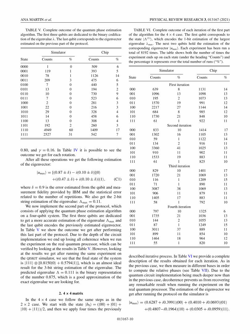
TABLE V. Complete outcome of the quantum phase estimationalgorithm. The first three qubits are dedicated to the binary codifica-tion of the eigenvalue λ. The last qubit corresponds to the eigenvectorestimated on the previous part of the protocol.

Simulator Chip

State Counts % Counts %

0000 1 0 509 60001 119 1 393 50010 78 1 1126 140011 209 3 475 60100 7 0 440 50101 13 0 194 20110 10 0 730 90111 7 0 523 61000 2 0 281 31001 22 0 216 31010 29 0 328 41011 14 0 458 61100 13 0 308 41101 192 2 260 31110 4949 60 1409 171111 2527 31 542 7

0.80, and γ = 0.16. In Table IV it is possible to see theoutcome we get for each rotation.

After all these operations we get the following estimationof the eigenvector:

|umax〉 = [(0.87 ± δ) − i(0.10 ± δ)]|0〉+((0.47 ± δ) + i(0.10 ± δ))|1〉, (C1)

where δ = 0.9 is the error estimated from the qubit and mea-surement fidelity provided by IBM and the statistical errorrelated to the number of repetitions. We also get the 2-bitstring estimation of the eigenvalue: �max = 0.11.

We now implement the second part of the protocol, whichconsists of applying the quantum phase estimation algorithmon a four-qubit system. The first three qubits are dedicatedto get a more accurate estimation of the eigenvalue �max andthe last qubit encodes the previously estimated eigenvector.In Table V we show the outcome we get after performingthis last part of the protocol. Due to the depth of the circuitimplementation we end up losing all coherence when we runthe experiment on the real quantum processor, which can beverified by looking at the results in Table V. However, lookingat the results we get after running the same experiment onthe QISKIT simulator, we see that the final state of the systemis |111〉 ⊗ [0.8150|0〉 + 0.5794|1〉], which is an almost idealresult for the 3-bit string estimation of the eigenvalue. Thepredicted eigenvalue � = 0.111 is the binary representationof the number 0.875, which is a good approximation of theexact eigenvalue we are looking for.

2. 4 × 4 matrix

In the 4 × 4 case we follow the same steps as in the2 × 2 case. We start with the state |b0〉 = (|00〉 + |01〉 +|10〉 + |11〉)/2, and then we apply four times the previously

TABLE VI. Complete outcome of each iteration of the first partof the algorithm for the 4 × 4 case. The first qubit corresponds tothe state |�(1)〉, which encodes the 1-bit estimation of the largesteigenvalue λmax. The next two qubits hold the estimation of thecorresponding eigenvector |umax〉. Each experiment has been run atotal of 8192 times. The table shows both the number of times theexperiment ends up on each state (under the heading “Counts”) andthe percentage it represents over the total number of runs (“%”).

Simulator Chip

State Counts % Counts %

First iteration000 639 8 1131 14001 1096 13 1098 13010 195 2 1073 13011 1570 19 991 12100 2217 27 1144 14101 684 8 985 12110 1730 21 848 10111 61 1 922 11

Second iteration000 833 10 1414 17001 1302 16 1105 13010 59 1 1122 14011 134 2 916 11100 3360 41 1025 13101 910 11 902 11110 1533 19 883 11111 61 1 825 10

Third iteration000 829 10 1401 17001 1720 21 1069 13010 116 1 1209 15011 71 1 890 11100 3087 38 1069 13101 906 11 879 11110 1405 17 883 11111 58 1 792 10

Fourth iteration000 797 10 1325 6001 1735 21 1036 13010 144 2 1055 13011 87 1 1249 15100 3011 37 889 11101 899 11 854 10110 1464 18 964 12111 55 1 820 10

described iterative process. In Table VI we provide a completedescription of the results obtained for each iteration. As inthe previous case, we then measure in different bases in orderto compute the relative phases (see Table VII). Due to thequantum circuit implementation being much deeper now thanin the previous case, decoherence prevents us from recoveringany remarkable result when running the experiment on thereal quantum processor. The estimation of the eigenvector weget after running the protocol on the simulator is

|umax〉 = (0.6287 + i0.3991)|00〉 + (0.4010 + i0.0693)|01〉+(0.4807−i0.1964)|10〉 + (0.0305 + i0.0959)|11〉.

013167-10

TOWARD PRICING FINANCIAL DERIVATIVES WITH AN … PHYSICAL REVIEW RESEARCH 3, 013167 (2021)

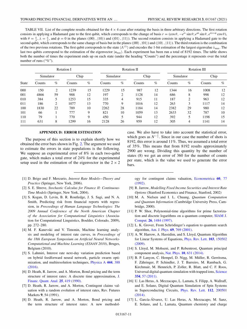
TABLE VII. List of the complete results obtained for the 4 × 4 case after rotating the basis in three arbitrary directions. The first rotationconsists in applying a Hadamard gate to the first qubit, which corresponds to the change of basis r = (cos θ, −eiλ sin θ ; eiφ sin θ, ei(λ+φ cos θ ),with θ = π

4 , λ = π

2 , and φ = 0 in the planes (|00〉 , |10〉) and (|01〉 , |11〉). The second rotation consists in applying a Hadamard gate to thesecond qubit, which corresponds to the same change of basis but in the planes (|00〉 , |01〉) and (|10〉 , |11〉). The third rotation is the combinationof the two previous rotations. The first qubit corresponds to the state |�(1)〉 and encodes the 1-bit estimation of the largest eigenvalue λmax. Thelast two qubits correspond to the estimation of the eigenvector |umax〉. Each experiment has been run a total of 8192 times. The table showsboth the number of times the experiment ends up on each state (under the heading “Counts”) and the percentage it represents over the totalnumber of runs (“%”).

Rotation I Rotation II Rotation III

Simulator Chip Simulator Chip Simulator Chip

State Counts % Counts % Counts % Counts % Counts % Counts %

000 150 2 1239 15 1229 15 987 12 1344 16 1008 12001 4866 59 988 12 197 2 1128 14 686 8 998 12010 384 5 1253 15 335 4 915 11 187 2 963 12011 186 2 1077 13 770 9 1016 12 263 3 1117 14100 1830 22 789 10 2262 28 1184 14 2382 29 980 12101 66 1 777 9 821 10 1059 13 2633 32 787 10110 79 1 770 9 450 5 944 12 392 5 1198 15111 631 8 1299 16 2128 26 959 12 305 4 1141 14

APPENDIX D: ERROR ESTIMATION

The purpose of this section is to explain shortly how weobtained the error bars shown in Fig. 2. The argument we usedto estimate the errors in state populations is the following.We suppose an experimental error of 8% in each two-qubitgate, which makes a total error of 24% for the experimentalsetup used in the estimation of the eigenvector in the 2 × 2

case. We also have to take into account the statistical error,which goes as N− 1

2 . Since in our case the number of shots is8192, this error is around 11%. Thus, we assumed a total errorof 35%. This means that from 8192 results approximately2900 are wrong. Dividing this quantity by the number ofstates (8) we get an error of 360 for the number of countsper state, which is the value we used to generate the errorbars.

[1] D. Brigo and F. Mercurio, Interest Rate Models—Theory andPractice (Springer, New York, 2006).

[2] S. E. Shreve, Stochastic Calculus for Finance II: Continuous-Time Models (Springer, New York, 2004).

[3] S. Kogan, D. Levin, B. R. Routledge, J. S. Sagi, and N. A.Smith, Predicting risk from financial reports with regres-sion, in Proceedings of Human Language Technologies: The2009 Annual Conference of the North American Chapterof the Association for Computational Linguistics (Associa-tion for Computational Linguistics, Boulder, Colorado, 2009),pp. 272–280.

[4] M. F. Kanevski and V. Timonin, Machine learning analy-sis and modeling of interest rate curves, in Proceedings ofthe 18th European Symposium on Artificial Neural Networks-Computational and Machine Learning (ESAAN 2010), Bruges,Belgium (2010).

[5] S. Lahmiri, Interest rate next-day variation prediction basedon hybrid feedforward neural network, particle swarm opti-mization, and multiresolution techniques, Physica A 444, 388(2016).

[6] D. Heath, R. Jarrow, and A. Morton, Bond pricing and the termstructure of interest rates: A discrete time approximation, J.Financ. Quant. Anal. 25, 419 (1990).

[7] D. Heath, R. Jarrow, and A. Morton, Contingent claims val-uation with a random evolution of interest rates, Rev. FuturesMarkets 9, 54 (1991).

[8] D. Heath, R. Jarrow, and A. Morton, Bond pricing andthe term structure of interest rates: A new methodol-

ogy for contingent claims valuation, Econometrica 60, 77(1992).

[9] R. Jarrow, Modelling Fixed Income Securities and Interest RateOptions (Stanford Economics and Finance, Stanford, 2002)

[10] M. A. Nielsen and I. L. Chuang, Quantum Computationand Quantum Information (Cambridge University Press, Cam-bridge, 2000).

[11] P. W. Shor, Polynomial-time algorithms for prime factoriza-tion and discrete logarithms on a quantum computer, SIAM J.Comput. 26, 1484 (1997).

[12] L. K. Grover, From Schrödinger’s equation to quantum searchalgorithm, Am. J. Phys. 69, 769 (2001).

[13] A. W. Harrow, A. Hassidim, and S. Lloyd, Quantum Algorithmfor Linear Systems of Equations, Phys. Rev. Lett. 103, 150502(2009).

[14] S. Lloyd, M. Mohseni, and P. Rebentrost, Quantum principalcomponent analysis, Nat. Phys. 10, 631 (2014).

[15] B. P. Lanyon, C. Hempel, D. Nigg, M. Müller, R. Gerritsma,F. Zähringer, P. Schindler, J. T. Barreiro, M. Rambach, G.Kirchmair, M. Hennrich, P. Zoller, R. Blatt, and C. F. Roos,Universal digital quantum simulation with trapped ions, Science334, 57 (2011).

[16] U. Las Heras, A. Mezzacapo, L. Lamata, S. Filipp, A. Wallraff,and E. Solano, Digital Quantum Simulation of Spin Systemsin Superconducting Circuits, Phys. Rev. Lett. 112, 200501(2014).

[17] L. García-Álvarez, U. Las Heras, A. Mezzacapo, M. Sanz,E. Solano, and L. Lamata, Quantum chemistry and charge

013167-11

ANA MARTIN et al. PHYSICAL REVIEW RESEARCH 3, 013167 (2021)

transport in biomolecules with superconducting circuits, Sci.Rep. 6, 27836 (2016).

[18] A. Kandala, A. Mezzacapo, K. Temme, M. Takita, M. Brink,J. M. Chow, and J. M. Gambetta, Hardware-efficient variationalquantum eigensolver for small molecules and quantum mag-nets, Nature 549, 242 (2017).

[19] J. Argüello-Luengo, A. González-Tudela, T. Shi, P. Zoller, andJ. I. Cirac, Analog quantum chemistry simulation, Nature 574,215 (2019).

[20] R. Babbush, D. W. Berry, J. R. McClean, and H. Neven,Quantum simulation of chemistry with sublinear scaling to thecontinuum, npj Quantum Inf. 5, 92 (2019).

[21] N. Klco, E. F. Dumitrescu, A. J. McCaskey, T. D. Morris, R. C.Pooser, M. Sanz, E. Solano, P. Lougovski, and M. J. Savage,Quantum-classical computation of Schwinger model dynamicsusing quantum computers, Phys. Rev. A 98, 032331 (2018).

[22] J. Preskill, Simulating quantum field theory with a quantumcomputer, arXiv:1811.10085.

[23] A. Mezzacapo, M. Sanz, L. Lamata, I. L. Egusquiza, S. Succi,and E. Solano, Quantum simulator for transport phenomena influid flows, Sci. Rep. 5, 13153 (2015).

[24] U. Alvarez-Rodriguez, M. Sanz, L. Lamata, and E. Solano,Biomimetic cloning of quantum observables, Sci. Rep. 4, 4910(2014).

[25] U. Alvarez-Rodriguez, M. Sanz, L. Lamata, and E. Solano,Quantum artificial life in quantum technologies, Sci. Rep. 6,20956 (2016).

[26] U. Alvarez-Rodriguez, M. Sanz, L. Lamata, and E. Solano,Quantum artificial life in an IBM quantum computer, Sci. Rep.8, 14793 (2018).

[27] B. E. Baaquie, Quantum Finance Hamiltonians and Path In-tegrals for Options (Cambridge University Press, Cambridge,2004).

[28] R. Orús, S. Mugel, and E. Lizaso, Forecasting financial crasheswith quantum computing, Phys. Rev. A 99, 060301 (2019).

[29] P. Rebentrost, B. Gupt, and T. R. Bromley, Quantum compu-tational finance: Monte Carlo pricing of financial derivatives,Phys. Rev. A 98, 022321 (2018).

[30] R. Orús, S. Mugel, and E. Lizaso, Quantum computingfor finance: Overview and prospects, Rev. Phys. 4, 100028(2019).

[31] J. Gonzalez-Conde, A. Rodríguez-Rozas, E. Solano, and M.Sanz, Pricing financial derivatives with exponential quantumspeedup, arXiv:2101.04023.

[32] N. Stamatopoulos, D. J. Egger, Y. Sun, C. Zoufal, R. Iten, N.Shen, and S. Woerner, Option pricing using quantum comput-ers, Quantum 4, 291 (2020).

[33] D. Venturelli and A. Kondratyev, Reverse quantum annealingapproach to portfolio optimization problems, Quantum Mach.Intell. 1, 17 (2019).

[34] S. Woerner and D. J. Egger, Quantum risk analysis, npjQuantum Inf. 5, 15 (2019).

[35] Y. Ding, J. Gonzalez-Conde, L. Lamata, J. D. Martín-Guerrero,E. Lizaso, S. Mugel, X. Chen, R. Orús, E. Solano, and M. Sanz,,Towards prediction of financial crashes with a D-Wave quantumcomputer, arXiv:1904.05808.

[36] P. Wilmott, Paul Wilmott Introduces Quantitative Finance (Wi-ley, New York, 2007).

[37] J. Preskill, Quantum computing in the NISQ era and beyond,Quantum 2, 79 (2018).

[38] D. W. Berry, G. Ahokas, R. Cleve, and B. C. Sanders, Effi-cient quantum algorithms for simulating sparse Hamiltonians,Commun. Math. Phys. 270, 359 (2007).

[39] A. M. Childs, On the relationship between continuous- anddiscrete-time quantum walk, Commun. Math. Phys. 294, 581(2010).

[40] G. Aleksandrowicz, T. Alexander, P. Barkoutsos, L. Bello, Y.Ben-Haim, D. Bucher, F. J. Cabrera-Hernádez, J. Carballo-Franquis, A. Chen, Ch.-F. Chen, J. M. Chow, A. D. Córcoles-Gonzales, A. J. Cross, A. Cross, J. Cruz-Benito, C. Culver,S. De La Puente González, E. De La Torre, D. Ding,E. Dumitrescu, I. Duran, P. Eendebak, M. Everitt, I. FaroSertage, A. Frisch, A. Fuhrer, J. Gambetta, B. Godoy Gago, J.Gomez-Mosquera, D. Greenberg, I. Hamamura, V. Havlicek, J.Hellmers, L. Herok, H. Horii, S. Hu, T. Imamichi, T. Itoko, A.Javadi-Abhari, N. Kanazawa, A. Karazeev, K. Krsulich, P. Liu,Y. Luh, Y. Maeng, M. Marques, F. J. Martín-Fernández, D. T.McClure, D. McKay, S. Meesala, A. Mezzacapo, N. Moll, D.Moreda Rodríguez, G. Nannicini, P. Nation, P. Ollitrault, L. J.O’Riordan, H. Paik, J. Pérez, A. Phan, M. Pistoia, V. Prutyanov,M. Reuter, J. Rice, A. Rodríguez Davila, R. H. Putra Rudy, M.Ryu, N. Sathaye, C. Schnabel, E. Schoute, K. Setia, Y. Shi, A.Silva, Y. Siraichi, S. Sivarajah, J. A. Smolin, M. Soeken, H.Takahashi, I. Tavernelli, C. Taylor, P. Taylour, K. Trabing, M.Treinish, W. Turner, D. Vogt-Lee, C. Vuillot, J. A. Wildstrom,J. Wilson, E. Winston, C. Wood, S. Wood, S. Wörner, I. Y.Akhalwaya, and C. Zoufal, QISKIT: An open-source frameworkfor quantum computing, 2019, https://github.com/Qiskit.

[41] A. Kandala, K. Temme, A. D. Corcoles, A. Mezzacapo, J. M.Chow, and J. M. Gambetta, Error mitigation extends the com-putational reach of a noisy quantum processor, Nature 567, 491(2019).

[42] K. Temme, S. Bravyi, and J. M. Gambetta, Error Mitigation forShort-Depth Quantum Circuits, Phys. Rev. Lett. 119, 180509(2017).

[43] A. Dewes, F. R. Ong, V. Schmitt, R. Lauro, N. Boulant,P. Bertet, D. Vion, and D. Esteve, Characterization of aTwo-Transmon Processor with Individual Single-Shot QubitReadout, Phys. Rev. Lett. 108, 057002 (2012).

[44] https://github.com/amartinfer/QPCA.git.

013167-12