Toward a unified theory of spatiotemporal processingin the retina

Paolo Gaudiano

Boston University, Department of Cognitive & Neural Systems111 Cummington Street, Boston, MA 02215 USA

Appears in: Carpenter, G., and Grossberg, S. (Eds.) Neural Networks for Visionand Image Processing. Ch.8, 195–220, MIT Press, 1992.

1

Toward a unified theory of spatiotemporal processing in the retina

Paolo Gaudiano

Boston University, Department of Cognitive & Neural Systems111 Cummington Street, Boston, MA 02215 USA

Abstract

Why do stabilized images fade? How can X cells in the retina respond linearly to a broad range ofspatiotemporal stimulation functions in spite of possible nonlinear preprocessing? Why have models ofspatial vision that utilize static images and assume linearity of preprocessing led to reasonable results inspite of the two questions above? This chapter introduces the push-pull shunting network, a model ofspatiotemporal visual processing that resolves these and other controversial findings. Development of themodel is based on an analysis of the spatial and temporal response characteristics of networks of neuronsthat obey membrane equations. The resulting architecture is structurally similar to the mammalian retina,requiring a mechanism for temporal adaptation analogous to photoreceptors, followed by cells of oppositepolarity analogous to on and off bipolar cells, and finally a layer of ganglion cells that summate bipolarcell inputs. The model predicts that X and Y cells consist of the same neural mechanism acting in differentparametric regimes. In agreement with morphological and physiological data, analyses and numericalsimulations show that an increase in receptive field center size changes the model’s response from X-liketo Y-like. This functional duality results from mathematical properties of the push-pull shunting network,which can selectively enhance sustained or transient response components on the basis of RF morphology.The model also explains how it is possible for X cells to respond linearly to a broad range of spatial andtemporal modulation functions in spite of arbitrary nonlinear preprocessing. Finally, in general agreementwith biological data, the model predicts that stationary images lead to loss of instantaneous contrast atequilibrium, i.e., that stabilized images fade, as an unavoidable side effect of photoreceptor adaptation.

1 Introduction

The retina, owing to its accessibility and to its fundamental role in the initial transduction oflight into neural signals, is arguably the most extensively studied neural structure in vision. Theanatomical structure of the retina has been known for almost exactly one century, beginning with thework of Ramon y Cajal in the late nineteenth century. It was not until approximately 50 years laterthat the technology became available for recording of individual cell activity, allowing researchersto gain insights on the information carried by neurons in the retina. Since that time detaileddescriptions have been given for the physiological, pharmacological, and functional properties ofmost classes of retinal cells. In spite of these advances, a unified understanding of the functionalrole of the processing carried out in the retina is still lacking.

In this chapter I introduce the push-pull shunting network, which was designed as a theoreticalmodel of spatiotemporal information processing by networks of neurons that obey membrane, orshunting, equations (Grossberg, 1970; Sperling, 1970; Sperling and Sondhi, 1968). I will showthat owing to the nonnegative nature of luminance signals, feed-forward shunting neural networkmodels are subject to an inescapable trade-off between accurate processing in the spatial andtemporal domains. Accurate processing in both domains can be achieved by extending the modelto include a total of three layers of feed-forward processing. The resulting model’s architecture

2

is structurally analogous to the feed-forward retinal circuit connecting photoreceptors to retinalganglion cells (RGCs) through pairs of push-pull bipolar cells. This analogy is confirmed throughcomputer simulations showing that the model’s output layer exhibits many properties observed incat RGCs.

In addition to qualitatively reproducing experimental data on retinal cells, the model is ableto resolve a number of controversial experimental and theoretical findings, and offers a unifiedfunctional explanation for the retina’s role as the first stage of spatiotemporal visual processing inbiological systems.

This chapter begins with a brief description of the anatomical and functional organization ofthe mammalian retina in Section 2, with a brief summary of the properties of two functionalclasses of cat retinal ganglion cells known as X and Y cells in Section 3. This is followed by twosections outlining a number of unresolved and controversial issues on retinal processing. Section 6introduces the shunting network on which this model is based, while Section 7 motivates theaddition of a push-pull mechanism for accurate spatiotemporal processing. Sections 8–11 presentthe push-pull shunting equation and a necessary model of temporal adaptation. Following a numberof simulation results in Sections 12–15, the chapter concludes by summarizing the properties ofthe model, discussing the controversial experimental findings presented in earlier sections, andoutlining a number of predictions and future applications of the model.

2 Anatomy and physiology of the retina

The retina of all vertebrates is organized into three cellular (or nuclear) layers and two synaptic(or plexiform) layers (Dowling, 1987). Information flows from the photoreceptors, through a layerof bipolar cells, and finally through the retinal ganglion cells (RGCs), whose axons project via theoptic nerve to subcortical and cortical areas. In addition to the feed-forward information processingcarried out by these three cell types, there exist two classes of cells, horizontal cells and amacrinecells, that carry signals laterally through the retina for additional processing.

Although there is general agreement that retinal cells can be subdivided into these broad classes,morphological and anatomical studies have shown the existence of a great number of cell typeswithin each class, including dozens of RGC and amacrine cell types (e.g., Kolb et al., 1981).

In addition to morphological and anatomical classification schemes, physiological studies haveshown the existence of distinct, broad functional classes. Kuffler (1953) and Barlow (1953) firstreported the existence of two RGC classes: on-center (ON) and off-center (OFF) cells. Both typeshave a concentrically-organized receptive field consisting of a central region and a surroundingannulus of opposite polarity. Presentation of a light stimulus over the receptive field center causesincreased activation for ON cells, and decreased activation for OFF cells. Conversely, stimulationof the receptive field surround decreases activation in the ON cells, and increases activation in OFFcells. The distinct response characteristics of ON and OFF RGCs appear to originate in the bipolarcell layer (Werblin and Dowling, 1969).

An additional, independent functional classification scheme was proposed by Enroth-Cugelland Robson (1966), who reported the existence of two RGC classes on the basis of spatiotemporalresponse characteristics: X cells, which respond to inputs in a sustained fashion, and appear tolinearly summate luminance signals throughout their receptive field; and Y cells, which respondto inputs in a transient fashion, and exhibit a more complicated, nonlinear spatial summation ofluminance signals throughout their receptive field. This classification has been supported and

3

LINEAR PREPROCESSING

0 90 180 270 0 90 180 270 0

(b)(a) X Y

Figure 1: (a): The null test. Left column represents response of an X cell to introduction andwithdrawal of a sinusoidal grating. Right column represents response of a Y cell to same stimulusconditions. See text for details. Reprinted with permission from Enroth-Cugell and Robson (1966).(b): Linear preprocessing of a temporally square-wave modulated sinusoidal grating leads to exactcancellation of input increments (hatched area) and decrements (stippled area) for cells locatedat �90� spatial phase relative to the sinusoidal grating.

extended through a number of physiological and anatomical studies, and a relationship has beenestablished between the morphological classes of alpha and beta ganglion cells, respectively, andthe functional classes of Y and X cells (Boycott and Wassle, 1974; Cleland and Levick, 1974;Fukuda et al., 1984; Hochstein and Shapley, 1976a,b; Saito, 1983).

3 An overview of X and Y retinal ganglion cells

The functional distinctions between X and Y cells reported by Enroth-Cugell and Robson (1966)were revealed through stimulation with temporally modulated spatial patterns. In these experi-ments, the activity of ganglion cells in response to such patterns was recorded in the optic nerve.The patterns were projected on a screen located in front of paralyzed cats, in a way that allowedaccurate control of the location of the stimulus pattern relative to the receptive field center of thecell being recorded.

A primary distinction between X and Y responses was found through what is referred to as thenull test, which is carried out in the following manner: the response of a ganglion cell is recordedwhile the projected image of a sinusoidal grating is turned on and off, i.e., is modulated in timeby a square wave of fixed temporal frequency. The sinusoidal spatial modulation is such that theaverage luminance of the grating superimposed on the background is equal to the luminance of thebackground alone. Measurement of the cell’s response to such spatiotemporal input modulation isrepeated as the grating’s spatial phase relative to the cell’s receptive field center is systematicallyvaried across trials.

As shown in Fig. 1a, two characteristics distinguish X and Y cells. First, as shown in the top

4

and third rows, the response of X cells (left column) to introduction and withdrawal of a gratingat zero or 180 degrees spatial phase consists of a primarily sustained component, whereas that ofY cells (right column) consists of primarily transient components. The other noticeable differencebetween X and Y cells is that for an X cell it is generally possible to find two distinct relative spatialphases, usually at �90�, at which no response is elicited by grating onset or offset (left column,second and fourth rows from the top of Fig. 1a). On the other hand, at a spatial phase of �90�the Y cell exhibits an on-off or frequency doubling response, that is, it exhibits a positive goingresponse to both onset and offset of the grating (right column, second and fourth rows).

The existence of null responses at�90� in X cells indicates that the sudden decrease in input toone side of the cell’s receptive field exactly cancels the concomitant increase in input to the otherside of the receptive field, as illustrated in Fig. 1b. As discussed below, these results thereforesuggest that X cells perform linear spatial summation over the extent of their receptive field, whileY cells perform a more complex form of nonlinear spatial summation.

Hochstein and Shapley (1976a,b) confirmed and extended the X/Y classification on the basis ofthe null test. They found that the linear/nonlinear classification holds for a wide range of temporalfrequency of modulation and for various types of spatial and temporal waveform, which led themto the hypothesis that the distinct behavior of X and Y cells implies different underlying retinalcircuits. Specifically, these authors proposed that the receptive field of both X and Y cells includeslinear center and surround mechanisms of the type proposed by Rodieck (1965), but that the Y cellreceptive field further includes small nonlinear subunits that overlap both the receptive field centerand surround.

4 Some unresolved experimental findings on X and Y cells

The findings outlined in the previous section have been the basis of much experimental andtheoretical work. However, there are a number of issues that remain unclear and have not beensatisfactorily explained. This includes not only issues on retinal processing, but also on theimportance of the retina as the first processing stage in the visual system.

Of great importance to many vision researchers is the issue of linearity: a number of visionmodels, both retinal and cortical, assume that retinal elements behave approximately linearly. Inpartial support of this assumption, Enroth-Cugell and Robson (1966) noted that the existence ofnull phases in X cells “... implies either that the signals from photoreceptors are linearly relatedto their illumination or that they are non-linearly related in a way which is symmetrical about themean illuminance.” These authors concluded that “the latter alternative can be ruled out by theobservation that the null positions for grating patterns are not changed when the mean luminanceis changed” (p. 524-525). In other words, the seemingly linear behavior of X cells regardless ofaverage luminance and contrast forced these authors to conclude that the response of photoreceptorsand bipolar cells must be linearly related to input intensity. The necessity of this conclusion isillustrated by Fig. 2, in which hypothetical nonlinear preprocessing mechanisms are shown to affectthe ability of subsequent stages (such as X cells) to carry out linear spatial summation.

However, it is known that photoreceptor response is not linearly related to luminance; photore-ceptors exhibit temporal adaptation that leads to a static nonlinear compression of the input range(e.g., Dowling, 1987; Rushton, 1958). From a functional point of view, it is important that thephotoreceptors be able to compress the input into a finite range, since any information that is lostat the photoreceptors cannot be recovered at later stages. Such a static nonlinearity could prevent

5

0 90 180 270 0 90 180 270 0

(b): TRANSIENT NONLINEARITY

0 90 180 270 0 90 180 270 0

(a): STATIC NONLINEARITY

Figure 2: The effect of hypothetical static and transient nonlinear preprocessing on the X cell’sability to exhibit null responses at �90� when stimulated by a square-wave modulated sinusoidalgrating. Each plot illustrates the input reaching various parts of the X cell’s receptive field as aspatial sinusoidal grating is contrast-reversed. The dashed and solid lines, respectively, representthe grating just before and just after contrast reversal. (a): Static nonlinear preprocessing maydistort the sinusoidal distribution depending on average input and contrast, so that input incrementsand decrements at �90� may not cancel out, as indicated by hatched and stippled areas. (b) Atransient nonlinearity may rapidly equilibrate to approximate linearity, but the initial nonlineardistortion (thick solid line) should prevent cancellation at �90� immediately following contrastreversal.

linear spatial summation in the X cell, as diagrammed in Fig. 2a.In addition to this static, compressive nonlinearity it is known that photoreceptors and bipolar

cells exhibit transient overshoots and undershoots to sudden input changes. Such transients arethe result of each photoreceptor trying to adjust its dynamic range in response to local changes ininput intensity. The purpose of these adjustments, in principle, is to maintain each photoreceptorwithin the linear portion of its dynamic range. However, such adjustments cannot be instantaneous(see also Section 15), so that rapid input fluctuations may temporarily drive the photoreceptor intothe nonlinear portion of its dynamic range, until the adaptation mechanism can drive it back intothe linear range. Hence photoreceptors should exhibit transient nonlinearities in response to rapidtemporal fluctuations. This type of transient nonlinearity is diagrammed in Fig. 2b, which portraysthe responses of hypothetical photoreceptors to a counterphase-flickered sinusoidal grating. Asshown in this figure, the photoreceptors’ responses immediately following contrast reversal canlead to a nonlinear distortion of the spatial sinusoidal distribution, which may quickly converge toa more linear response. However, such a transient nonlinearity should prevent exact cancellation inthe X cell response to square-wave temporal modulation of a sinusoidal grating. In other words, onewould not expect null responses at�90� spatial phase when the grating is square-wave modulated,as in the classical experiments of Enroth-Cugell and Robson (1966). How can X cells exhibitseemingly linear behavior in spite of nonlinear preprocessing?

Equally puzzling is the experimental finding that whereas X cells behave linearly even inresponse to fast temporal modulation, it has been noted that rapid changes in the spatial modulationfunction can result in X cell nonlinear behavior. For example, X cells sometimes exhibit on-offresponses to temporal modulation of a bipartite field, or contrast edge. Is this behavior the resultof a mechanism similar to the one generating on-off responses in Y cells? If so, why does thismechanism only affect X cell responses to a particular type of spatial modulation?

6

5 Some general issues in spatiotemporal processing

Resolution of the controversial findings outlined in the last section requires simultaneous analysis ofthe spatial and temporal response characteristics of retinal ganglion cells. However, even thoughdata have shown an inextricable tie between RGC responses in the space and time domains, amajority of existing models of spatial vision assume that the incoming image is stabilized, i.e. it isconstant in time; conversely, most models of RGC temporal response characteristics only considerindividual cells responding to carefully defined spatial stimuli.

The use of stabilized stimuli in spatial vision models is perplexing for two reasons: first, it hasbeen known for four decades that biological visual systems are unable to perceive stabilized images.Ditchburn and Ginsborg (1952) first reported that images stabilized with respect to the retina rapidlyfade, giving rise in a matter of seconds to perception of a uniform gray field (loss of contrast), afinding that appears to hold for most biological visual systems. Second, most physiological andpsychophysical experiments make use of stimuli that are modulated both in space and in time.1

Therefore models that preclude the possibility of temporal modulation cannot be applied to themajority of physiological and psychophysical data.

This chapter introduces a model of spatiotemporal information processing that was developedto address these and related questions. The next section provides an overview of prior work onwhich the model is based.

6 The feed-forward shunting network

The present work is based on the feed-forward shunting network, which consists of continuous-time neurons obeying membrane equations. Membrane conductance to different ionic species ismodulated by the input through a center-surround receptive field structure. Historically, the termshunt as applied to neural networks refers to the presence of multiplicative saturation terms inthe equation describing membrane potential (Furman, 1965; Grossberg, 1970, 1973; Hodgkin,1964; Sperling, 1970; Sperling and Sondhi, 1968). The present usage of the term shunt, based onGrossberg’s (1970) original formulation, is more general than in its physiological definition, in thesense that the shunting network can exhibit either divisive (multiplicative) or subtractive (additive)effects depending on the choice of parameters and the input intensity.

The simplest differential equation describing an on-center, off-surround shunting network(Fig. 3a) can be written as follows:dvidt = �Avi + (B � vi)Ii � (D + vi)Xk 6=i Ik. (1)Here vi represents the activation or potential (which are assumed to be proportional in this model)of the ith cell in the network; A is the rate of passive decay toward the resting potential (whichis assumed here to be zero); B and D represent the excitatory and inhibitory saturation points,respectively; Ii represents the excitatory contribution from the ith component of the input pattern tothe ith cell (on-center); and

Pk 6=i Ik represents the inhibitory contribution from all other componentsof the input pattern to the ith cell (off-surround). All parameters are assumed to be nonnegative.In the absence of inputs, activation vi decays to zero at a rate �Avi. Otherwise, (1) guarantees

1Note that because the human eye is constantly jittering, even those psychophysical experiments that involvefixation of a steady image result in a temporally modulated image at the retinal level.

7

(a) (b)

I i

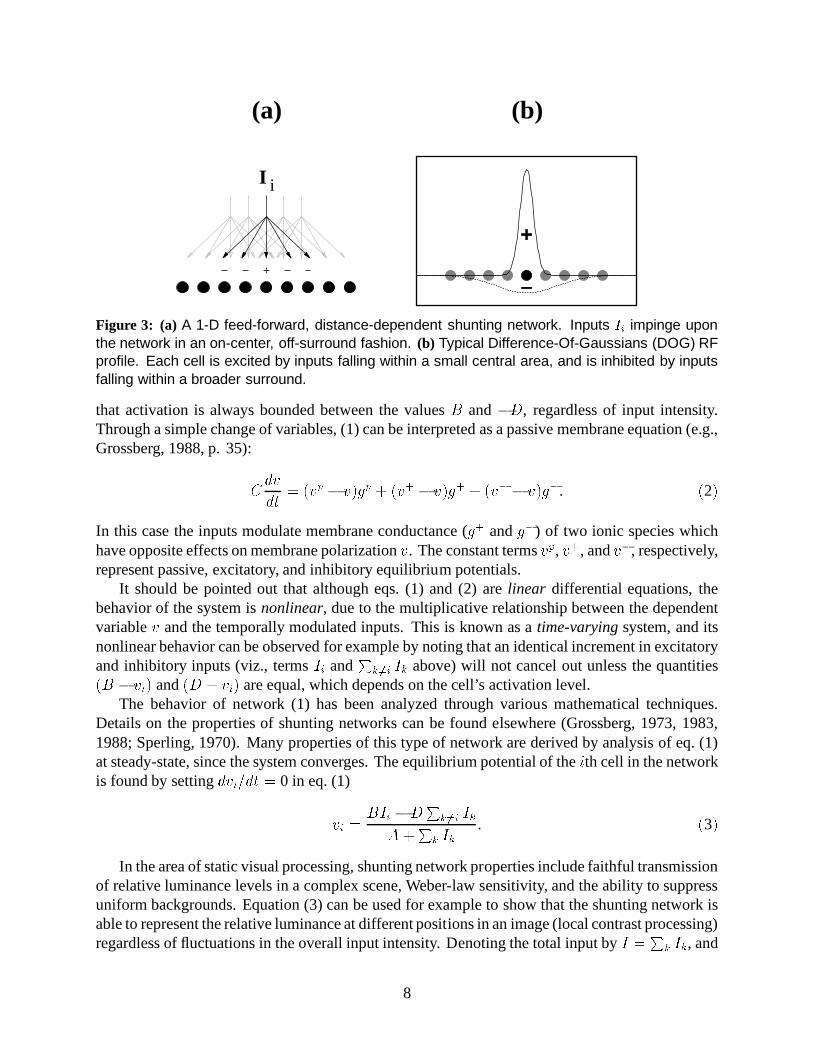
Figure 3: (a) A 1-D feed-forward, distance-dependent shunting network. Inputs Ii impinge uponthe network in an on-center, off-surround fashion. (b) Typical Difference-Of-Gaussians (DOG) RFprofile. Each cell is excited by inputs falling within a small central area, and is inhibited by inputsfalling within a broader surround.

that activation is always bounded between the values B and �D, regardless of input intensity.Through a simple change of variables, (1) can be interpreted as a passive membrane equation (e.g.,Grossberg, 1988, p. 35):C dvdt = (vp � v)gp + (v+ � v)g+ + (v� � v)g�. (2)In this case the inputs modulate membrane conductance (g+ and g�) of two ionic species whichhave opposite effects on membrane polarization v. The constant terms vp, v+, and v�, respectively,represent passive, excitatory, and inhibitory equilibrium potentials.

It should be pointed out that although eqs. (1) and (2) are linear differential equations, thebehavior of the system is nonlinear, due to the multiplicative relationship between the dependentvariable v and the temporally modulated inputs. This is known as a time-varying system, and itsnonlinear behavior can be observed for example by noting that an identical increment in excitatoryand inhibitory inputs (viz., terms Ii and

Pk 6=i Ik above) will not cancel out unless the quantities(B � vi) and (D + vi) are equal, which depends on the cell’s activation level.The behavior of network (1) has been analyzed through various mathematical techniques.

Details on the properties of shunting networks can be found elsewhere (Grossberg, 1973, 1983,1988; Sperling, 1970). Many properties of this type of network are derived by analysis of eq. (1)at steady-state, since the system converges. The equilibrium potential of the ith cell in the networkis found by setting dvi=dt = 0 in eq. (1)vi = BIi �DPk 6=i IkA+Pk Ik . (3)

In the area of static visual processing, shunting network properties include faithful transmissionof relative luminance levels in a complex scene, Weber-law sensitivity, and the ability to suppressuniform backgrounds. Equation (3) can be used for example to show that the shunting network isable to represent the relative luminance at different positions in an image (local contrast processing)regardless of fluctuations in the overall input intensity. Denoting the total input by I = Pk Ik, and

8

the relative input intensity at position i by �i = Ii=I , equation (3) can be rewritten asvi = (B +D)IA+ I ��i � DB +D� . (4)As long as the passive decay is small (A� I), equation (4) factorizes information about relativeinput size �i from overall intensity I , because activation vi is approximately proportional to�i � DB+D regardless of overall input intensity I . Grossberg (1980) has also shown that the regionof maximal sensitivity of a cell obeying (1) shifts without compression as the background intensityis parametrically increased. This is known as the shift property, which has been demonstratedexperimentally for certain classes of retinal cells (Werblin, 1971).

Similar results ensue when the center-surround mechanism consists of distinct, overlappingcenter and surround components, as shown in Fig. 3b. Equation (1) then becomesdvidt = �Avi + (B � vi)Xk C(k � i)Ik � (D + vi)Xk S(k � i)Ik. (5)

The distance-dependent termsC(k � i) and S(k � i) represent the center and surround mecha-nisms of the receptive field profile of each cell in the network. Most of the general results reportedhere are insensitive to the exact shape of the center and surround mechanisms. Where explicitclosed-form results are required these terms are described as Gaussians:C(k � i) = C exp

"�(k � i)2

2�2C #; S(k � i) = S exp

"�(k � i)2

2�2S #. (6)

Each Gaussian is described by its peak amplitude (C , S) and standard deviation (�C , �S). Theoverall receptive field shape is composed of the antagonistic excitatory center and inhibitorysurround Gaussians, and is thus referred to as a Difference-Of-Gaussians profile. Throughout thischapter it is assumed that �C < �S andC > S, which is representative of an on-center, off-surroundanatomy, though all results generalize to off-center on-surround anatomies as well.

7 Spatiotemporal analysis

An analysis of the shunting network’s response to spatiotemporal modulation revealed a tradeoffin the network’s ability to process information in space and time simultaneously. Details andsimulation results can be found elsewhere (Gaudiano, 1991a,b). Briefly, the conclusion stems fromthe realization that light, as a physical quantity, must be nonnegative. As a result the shuntingnetwork exhibits an asymmetry in its response to light increments and decrements. This can beseen from eq. (1), which shows that when inputs are increased the response of each neuron in thenetwork changes at a rate that depends both on the neuron’s activation level vi and on the size ofthe inputs Ij . On the other hand reducing all inputs to zero leaves the neuron’s activation to decaypassively at a rate that only depends on the neuron’s activation level vi and the decay constant A.

The space-time tradeoff is revealed in eq. (4) by noting that the shunting network’s ability toprocess relative luminance requires that A is much less than I , resulting in a slow passive decayin response to input decrements. Increasing the size of A relative to the other dynamic parameters(viz., B andD in eq. [1]) can partly compensate for this asymmetry, but only at the cost of reducingthat portion of the neuron’s dynamic range in which relative luminance is accurately processed.

9

(a) (b)I(t)

tv(t)

t

Input

Shunting cell response

Input

Push-pull RGC response

v(t)

I(t)

t

t

Figure 4: (a): The response of a shunting cell to whole-field sinusoidal modulation. (b): Theresponse of a push-pull shunting cell to similar whole-field sinusoidal modulation. See text fordetails.

Fig. 4a illustrates the response of a single neuron whose activation obeys eq. (5) to whole-fieldtemporal modulation of a 1-D luminance profile. When the input is first turned on (upper plot,solid line), the neuron’s activation (lower plot) rapidly rises, but subsequently shows little responseto the deep temporal modulation. The passive decay rate A in this example was chosen an order ofmagnitude larger than the positive saturation constant B. Such a large passive decay rate hampersthe shunting neuron of its reflectance processing ability, as illustrated in Fig. 4a by the dashedlines, which shows that a small increase in background intensity results in decreased responsemodulation.

Although the above results are based on the shunting formalism as it applies to luminancestimuli, nonnegative inputs must have similar asymmetrical effects on any model that prescribestime-dependent interactions between input and activation. For example, a similar problem canoccur in the control of limb movement: Bullock & Grossberg (1988; see also Gaudiano, 1991a)used a set of continuous-time equations to describe the behavior of a neural network for thegeneration and control of arm movement trajectories. It was found that if the neural commandsignal that causes muscle contraction is assumed to be nonnegative, then the muscle will contractat a variable rate that depends on the size of the signal, but will only be able to relax at a ratedetermined by a passive decay constant. The solution in that case was to postulate the existenceof agonist-antagonist muscle pairs coupled in a push-pull fashion, so that passive relaxation of theagonist muscle is accompanied by an active contraction of the antagonist muscle, and vice versa.Such agonist-antagonist interactions are of course ubiquitous in skeleto-muscular systems.

In analogy with this motor control problem, Gaudiano (1991a) first proposed that a similararrangement could take place in the visual system. Specifically, the asymmetry arising from thenonnegative nature of light can be corrected by means of two complementary input pathways to thenetwork, one signaling luminance increments, the other signaling luminance decrements. Together,these pathways allow the shunting network to track temporal modulation faithfully (Fig. 4b).

As mentioned in Section 2, such complementary pathways are known to exist in the parallelON and OFF retinal circuits (Barlow, 1953; Kuffler, 1953); thus one possibility is that signalsfrom the ON and OFF pathways interact recurrently to generate a response to increasing as well asdecreasing inputs. Although some evidence exists for feedback signals within the retina, this does

10

+ -

0

M

I (t)k

0

M

M-I (t)k

v (t)i

-D

B

0

+ -

I (t)k

L (t)k

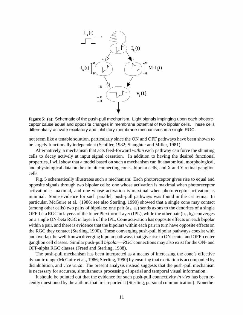
Figure 5: (a): Schematic of the push-pull mechanism. Light signals impinging upon each photore-ceptor cause equal and opposite changes in membrane potential of two bipolar cells. These cellsdifferentially activate excitatory and inhibitory membrane mechanisms in a single RGC.

not seem like a tenable solution, particularly since the ON and OFF pathways have been shown tobe largely functionally independent (Schiller, 1982; Slaughter and Miller, 1981).

Alternatively, a mechanism that acts feed-forward within each pathway can force the shuntingcells to decay actively at input signal cessation. In addition to having the desired functionalproperties, I will show that a model based on such a mechanism can fit anatomical, morphological,and physiological data on the circuit connecting cones, bipolar cells, and X and Y retinal ganglioncells.

Fig. 5 schematically illustrates such a mechanism. Each photoreceptor gives rise to equal andopposite signals through two bipolar cells: one whose activation is maximal when photoreceptoractivation is maximal, and one whose activation is maximal when photoreceptor activation isminimal. Some evidence for such parallel, push-pull pathways was found in the cat retina. Inparticular, McGuire et al. (1986; see also Sterling, 1990) showed that a single cone may contact(among other cells) two pairs of bipolars: one pair (a1, a2) sends axons to the dendrites of a singleOFF-beta RGC in layer a of the Inner Plexiform Layer (IPL), while the other pair (b1, b2) convergeson a single ON-beta RGC in layer b of the IPL. Cone activation has opposite effects on each bipolarwithin a pair, and there is evidence that the bipolars within each pair in turn have opposite effects onthe RGC they contact (Sterling, 1990). These converging push-pull bipolar pathways coexist withand overlap the well-known diverging bipolar pathways that give rise to ON-center and OFF-centerganglion cell classes. Similar push-pull bipolar!RGC connections may also exist for the ON- andOFF-alpha RGC classes (Freed and Sterling, 1988).

The push-pull mechanism has been interpreted as a means of increasing the cone’s effectivedynamic range (McGuire et al., 1986; Sterling, 1990) by ensuring that excitation is accompanied bydisinhibition, and vice versa. The present analysis instead suggests that the push-pull mechanismis necessary for accurate, simultaneous processing of spatial and temporal visual information.

It should be pointed out that the evidence for such push-pull connectivity in vivo has been re-cently questioned by the authors that first reported it (Sterling, personal communication). Nonethe-

11

less, the conclusions drawn in this section are based on general constraints of spatiotemporalprocessing of nonnegative signals, so that the present work predicts that such a push-pull mecha-nism should be found in the retina (see also the closing section in this chapter).

8 The push-pull shunting network

I next introduce a simple extension of eq. (5) that embodies the proposed push-pull mechanism,and analyze its spatiotemporal response. Detailed derivation of all results presented here can befound elsewhere (Gaudiano, 1991a,b). This section may be skipped on a first reading.

With reference to Fig. 5, let the input impinging upon each element of the shunting networkbe bounded between zero and a maximum level M . This constraint is valid on assumption thatinputs to the shunting network originate from layers of preprocessing elements that possess a finitedynamic range, as may result from photoreceptor adaptation. Each photoreceptor then gives riseto two signals, one that affects the excitatory mechanism of the target RGC through a depolarizingbipolar cell, and one that affects its inhibitory mechanism through a hyperpolarizing bipolar cell. Itis assumed that the same push-pull mechanism exists for cells comprising both the center and theantagonistic surround mechanisms. This does not preclude the possibility that center and surroundmechanisms be mediated by different cell classes: for example, amacrine cells may mediate thesurround mechanism, in which case it is assumed that these cells also receive parallel opponentinputs from push-pull bipolar cells.

If the bipolars act on a fast time scale relative to the photoreceptors, they can be lumpedinto equation (5) by addition of two terms to the input. Specifically, the excitatory inputthrough the receptive field center [

PC(k � i)Ik] is complemented by an opponent inhibitory input[PC(k � i) (M � Ik)], also through the receptive field center; likewise, the inhibitory surround

input [PS(k � i)Ik] is complemented by an opponent excitatory term [

PS(k � i) (M � Ik)]. Theresulting push-pull shunting equation isdvidt = �Avi + (B � vi) hXC(k � i)Ik +XS(k � i) (M � Ik)

i�(D + vi) hXS(k � i)Ik +XC(k � i) (M � Ik)i

, (7)

where Ik � M for all k. The equation shows that the center and surround each act on bothexcitatory and inhibitory channels, but in an opposing fashion.

Equation (7) can be rewritten as an integro-differential equation in space and time:@v(x; t)@t = �Av(x; t)+ �B�v(x; t)� �Z 1�1C(x��)I(�; t)d� + Z 1�1S(x��) �M�I(�; t)� d��� �D+v(x; t)� �Z 1�1S(x��)I(�; t)d� + Z 1�1C(x��) �M�I(�; t)� d�� (8)Equation (8) can be simplified when the input function is space-time separable, i.e., when it consistsof the product of two functions, one depending only on time, and the other depending only onspace: I(x; t) = I(x)m(t). (9)Many of the stimuli used for experimental measurements can be expressed as space-time separablefunctions, including for example sinusoidally or square-wave modulated spatial gratings, and drift-ing sinusoidal gratings. Other functions sometime lead to closed-form solutions of equation (8).

12

More generally, the response of equation (8) to an arbitrary function can be numerically inte-grated. All analytical results presented here are also simulated on the computer through numericalintegration of the discrete equation (7) above.

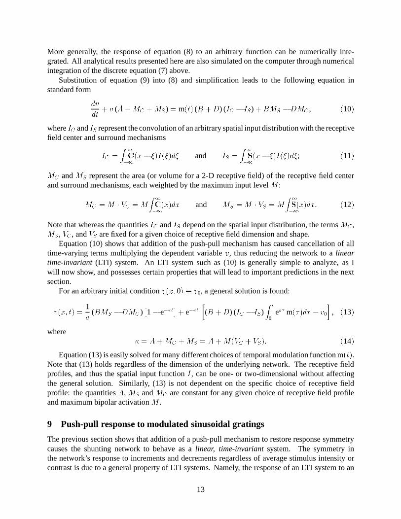
Substitution of equation (9) into (8) and simplification leads to the following equation instandard formdvdt + v (A+MC +MS ) = m(t) (B +D) (IC � IS)+BMS �DMC , (10)where IC and IS represent the convolution of an arbitrary spatial input distribution with the receptivefield center and surround mechanismsIC = Z 1�1C(x� �)I(�)d� and IS = Z 1�1S(x� �)I(�)d�; (11)MC and MS represent the area (or volume for a 2-D receptive field) of the receptive field centerand surround mechanisms, each weighted by the maximum input level M :MC =M � VC =MZ 1�1C(x)dx and MS =M � VS =MZ 1�1S(x)dx. (12)Note that whereas the quantities IC and IS depend on the spatial input distribution, the terms MC ,MS , VC , and VS are fixed for a given choice of receptive field dimension and shape.

Equation (10) shows that addition of the push-pull mechanism has caused cancellation of alltime-varying terms multiplying the dependent variable v, thus reducing the network to a lineartime-invariant (LTI) system. An LTI system such as (10) is generally simple to analyze, as Iwill now show, and possesses certain properties that will lead to important predictions in the nextsection.

For an arbitrary initial condition v(x; 0) � v0, a general solution is found:v(x; t) = 1a (BMS �DMC )�1� e�at�+ e�at �(B +D) (IC � IS)

Z t0

ea� m(� )d� + v0

�, (13)

where a = A+MC +MS = A+M(VC + VS). (14)Equation (13) is easily solved for many different choices of temporal modulation function m(t).

Note that (13) holds regardless of the dimension of the underlying network. The receptive fieldprofiles, and thus the spatial input function I , can be one- or two-dimensional without affectingthe general solution. Similarly, (13) is not dependent on the specific choice of receptive fieldprofile: the quantities A, MS and MC are constant for any given choice of receptive field profileand maximum bipolar activation M .

9 Push-pull response to modulated sinusoidal gratings

The previous section shows that addition of a push-pull mechanism to restore response symmetrycauses the shunting network to behave as a linear, time-invariant system. The symmetry inthe network’s response to increments and decrements regardless of average stimulus intensity orcontrast is due to a general property of LTI systems. Namely, the response of an LTI system to an

13

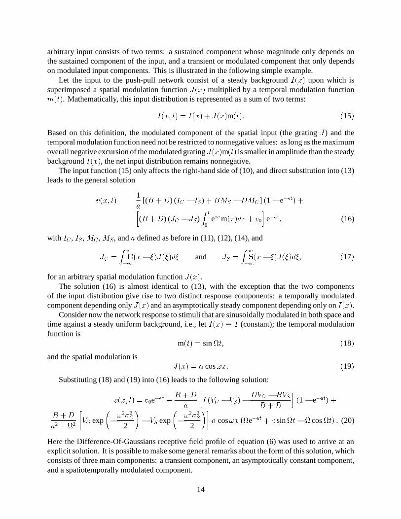
arbitrary input consists of two terms: a sustained component whose magnitude only depends onthe sustained component of the input, and a transient or modulated component that only dependson modulated input components. This is illustrated in the following simple example.

Let the input to the push-pull network consist of a steady background I(x) upon which issuperimposed a spatial modulation function J(x) multiplied by a temporal modulation functionm(t). Mathematically, this input distribution is represented as a sum of two terms:I(x; t) = I(x) + J(x)m(t): (15)Based on this definition, the modulated component of the spatial input (the grating J ) and thetemporal modulation function need not be restricted to nonnegative values: as long as the maximumoverall negative excursion of the modulated grating J(x)m(t) is smaller in amplitude than the steadybackground I(x), the net input distribution remains nonnegative.

The input function (15) only affects the right-hand side of (10), and direct substitution into (13)leads to the general solutionv(x; t) = 1a [(B +D) (IC � IS) +BMS �DMC ]

�1� e�at�+�

(B +D) (JC � JS)Z t

0ea�m(� )d� + v0

�e�at, (16)

with IC , IS , MC , MS , and a defined as before in (11), (12), (14), andJC = Z 1�1C(x� �)J(�)d� and JS = Z 1�1S(x� �)J(�)d�, (17)for an arbitrary spatial modulation function J(x).

The solution (16) is almost identical to (13), with the exception that the two componentsof the input distribution give rise to two distinct response components: a temporally modulatedcomponent depending only J(x) and an asymptotically steady component depending only on I(x).

Consider now the network response to stimuli that are sinusoidally modulated in both space andtime against a steady uniform background, i.e., let I(x) � I (constant); the temporal modulationfunction is

m(t) = sint, (18)and the spatial modulation is J(x) = � cos!x. (19)

Substituting (18) and (19) into (16) leads to the following solution:v(x; t) = v0e�at + B +Da �I (VC � VS )� DVC �BVSB +D � �1� e�at�+B +Da2 + 2

"VC exp

�!2�2C2

!� VS exp

�!2�2S2

!#� cos!x �e�at + a sint� cost� . (20)

Here the Difference-Of-Gaussians receptive field profile of equation (6) was used to arrive at anexplicit solution. It is possible to make some general remarks about the form of this solution, whichconsists of three main components: a transient component, an asymptotically constant component,and a spatiotemporally modulated component.

14

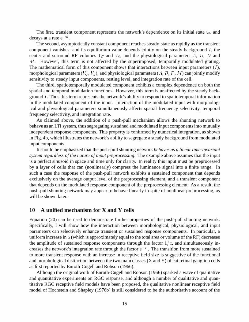
The first, transient component represents the network’s dependence on its initial state v0, anddecays at a rate e�at.

The second, asymptotically constant component reaches steady-state as rapidly as the transientcomponent vanishes, and its equilibrium value depends jointly on the steady background I , thecenter and surround RF volumes VC and VS , and the physiological parameters A, B, D andM . However, this term is not affected by the superimposed, temporally modulated grating.The mathematical form of this component shows that interactions between input parameters (I),morphological parameters (VC , VS), and physiological parameters (A,B,D, M ) can jointly modifysensitivity to steady input components, resting level, and integration rate of the cell.

The third, spatiotemporally modulated component exhibits a complex dependence on both thespatial and temporal modulation functions. However, this term is unaffected by the steady back-ground I . Thus this term represents the network’s ability to respond to spatiotemporal informationin the modulated component of the input. Interaction of the modulated input with morpholog-ical and physiological parameters simultaneously affects spatial frequency selectivity, temporalfrequency selectivity, and integration rate.

As claimed above, the addition of a push-pull mechanism allows the shunting network tobehave as an LTI system, thus segregating sustained and modulated input components into mutuallyindependent response components. This property is confirmed by numerical integration, as shownin Fig. 4b, which illustrates the network’s ability to segregate a steady background from modulatedinput components.

It should be emphasized that the push-pull shunting network behaves as a linear time-invariantsystem regardless of the nature of input preprocessing. The example above assumes that the inputis a perfect sinusoid in space and time only for clarity. In reality this input must be preprocessedby a layer of cells that can (nonlinearly) compress the luminance signal into a finite range. Insuch a case the response of the push-pull network exhibits a sustained component that dependsexclusively on the average output level of the preprocessing element, and a transient componentthat depends on the modulated response component of the preprocessing element. As a result, thepush-pull shunting network may appear to behave linearly in spite of nonlinear preprocessing, aswill be shown later.

10 A unified mechanism for X and Y cells

Equation (20) can be used to demonstrate further properties of the push-pull shunting network.Specifically, I will show how the interaction between morphological, physiological, and inputparameters can selectively enhance transient or sustained response components. In particular, auniform increase in a (which is approximately equal to the total area or volume of the RF) decreasesthe amplitude of sustained response components through the factor 1=a, and simultaneously in-creases the network’s integration rate through the factor e�at. The transition from more sustainedto more transient response with an increase in receptive field size is suggestive of the functionaland morphological distinction between the two main classes (X and Y) of cat retinal ganglion cellsas first reported by Enroth-Cugell and Robson (1966).

Although the original work of Enroth-Cugell and Robson (1966) sparked a wave of qualitativeand quantitative experiments on RGC response, and although a number of qualitative and quan-titative RGC receptive field models have been proposed, the qualitative nonlinear receptive fieldmodel of Hochstein and Shapley (1976b) is still considered to be the authoritative account of the

15

Y-cell’s receptive field. This model embodies the belief that different neural mechanisms mustcomprise the X and Y receptive fields.

The push-pull shunting network of eq. (7) instead provides a framework for a unified quantitativeexplanation of the behavior of both X and Y cells in response to spatiotemporally modulated inputs.Specifically, the interactions of the push-pull bipolar mechanism with the receptive field center andsurround components may give rise to X-like response characteristics for small receptive fieldprofiles, or Y-like response characteristics for larger receptive field profiles, in agreement withexperimental data linking X cells with beta cells, and Y cells with alpha cells (Cleland and Levick,1974; Fukuda et al., 1984; Saito, 1983).

In order to assess the validity of this claim it is first necessary to specify a mechanism capable oftemporal adaptation, that is, one that can adjust its dynamic range in response to input fluctuationsso as to compress a broad range of luminance signals into a bounded range of neural signals. Notethat in the absence of such a mechanism the push-pull shunting network is unable to simulate Xand Y cell data for at least two reasons: first, the model as it stands does not exhibit the overshootsand undershoots typically seen in X and Y cell response to sudden input fluctuations (e.g., Fig. 1).Second, if the input to the network were simply a linear copy of the luminance profile (such as thesinusoidal grating used above), then the network’s response should be purely linear, and nonlinearphenomena such as Y cell frequency doubling cannot be generated.

I will argue in the remainder of the chapter that the transient (overshoots and undershoots) andnonlinear components of X and Y cell responses arise through preprocessing in the photoreceptorand bipolar cell layers, and that the push-pull mechanism causes the ganglion cells to behave asclose to linear as possible in spite of nonlinearities in the preprocessing layers.

11 The photoreceptor model

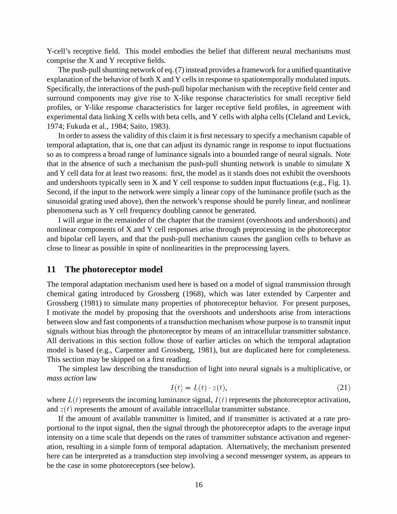
The temporal adaptation mechanism used here is based on a model of signal transmission throughchemical gating introduced by Grossberg (1968), which was later extended by Carpenter andGrossberg (1981) to simulate many properties of photoreceptor behavior. For present purposes,I motivate the model by proposing that the overshoots and undershoots arise from interactionsbetween slow and fast components of a transduction mechanism whose purpose is to transmit inputsignals without bias through the photoreceptor by means of an intracellular transmitter substance.All derivations in this section follow those of earlier articles on which the temporal adaptationmodel is based (e.g., Carpenter and Grossberg, 1981), but are duplicated here for completeness.This section may be skipped on a first reading.

The simplest law describing the transduction of light into neural signals is a multiplicative, ormass action law I(t) = L(t) � z(t), (21)where L(t) represents the incoming luminance signal, I(t) represents the photoreceptor activation,and z(t) represents the amount of available intracellular transmitter substance.

If the amount of available transmitter is limited, and if transmitter is activated at a rate pro-portional to the input signal, then the signal through the photoreceptor adapts to the average inputintensity on a time scale that depends on the rates of transmitter substance activation and regener-ation, resulting in a simple form of temporal adaptation. Alternatively, the mechanism presentedhere can be interpreted as a transduction step involving a second messenger system, as appears tobe the case in some photoreceptors (see below).

16

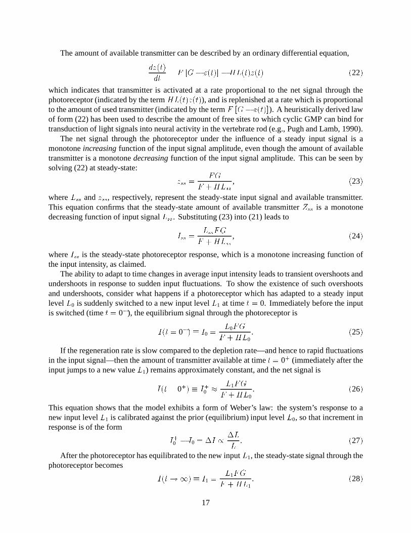
The amount of available transmitter can be described by an ordinary differential equation,dz(t)dt = F �G� z(t)��HL(t)z(t) (22)which indicates that transmitter is activated at a rate proportional to the net signal through thephotoreceptor (indicated by the term HL(t)z(t)), and is replenished at a rate which is proportionalto the amount of used transmitter (indicated by the term F �G� z(t)�). A heuristically derived lawof form (22) has been used to describe the amount of free sites to which cyclic GMP can bind fortransduction of light signals into neural activity in the vertebrate rod (e.g., Pugh and Lamb, 1990).

The net signal through the photoreceptor under the influence of a steady input signal is amonotone increasing function of the input signal amplitude, even though the amount of availabletransmitter is a monotone decreasing function of the input signal amplitude. This can be seen bysolving (22) at steady-state: zss = FGF +HLss , (23)where Lss and zss, respectively, represent the steady-state input signal and available transmitter.This equation confirms that the steady-state amount of available transmitter Zss is a monotonedecreasing function of input signal Lss. Substituting (23) into (21) leads toIss = LssFGF +HLss , (24)where Iss is the steady-state photoreceptor response, which is a monotone increasing function ofthe input intensity, as claimed.

The ability to adapt to time changes in average input intensity leads to transient overshoots andundershoots in response to sudden input fluctuations. To show the existence of such overshootsand undershoots, consider what happens if a photoreceptor which has adapted to a steady inputlevel L0 is suddenly switched to a new input level L1 at time t = 0. Immediately before the inputis switched (time t = 0�), the equilibrium signal through the photoreceptor isI(t = 0�) � I0 = L0FGF +HL0

. (25)If the regeneration rate is slow compared to the depletion rate—and hence to rapid fluctuations

in the input signal—then the amount of transmitter available at time t = 0+ (immediately after theinput jumps to a new value L1) remains approximately constant, and the net signal isI(t = 0+) � I+0 � L1FGF +HL0

. (26)This equation shows that the model exhibits a form of Weber’s law: the system’s response to anew input level L1 is calibrated against the prior (equilibrium) input level L0, so that increment inresponse is of the form I+0 � I0 = �I / �LL . (27)

After the photoreceptor has equilibrated to the new input L1, the steady-state signal through thephotoreceptor becomes I(t!1) � I1 = L1FGF +HL1

. (28)17

(a)

(b)

0

90

180

270

X Y

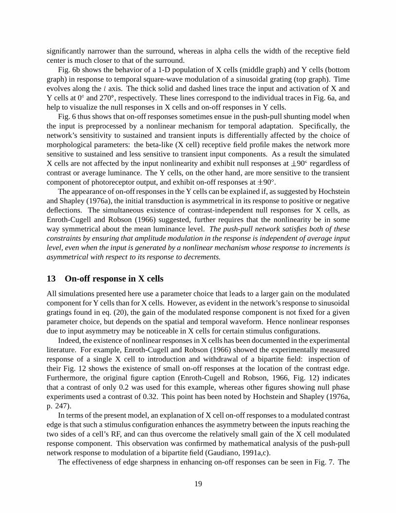
Figure 6: (a): Qualitative reproduction of thenull phase test data of Fig. 1. (b): Input andresponse for 1-D populations of simulated Xand Y cells. See text.

Input

0o

270o

Y RGC Response

X RGC Response

v(x,t)

v(x,t)

L(x,t)

x

x

x

t

t

t

IfL1 > L0, (26) and (28) jointly imply that I+0 > I1, which is indicative of a transient overshoot.A similar analysis shows that an undershoot will occur if L1 < L0.

It is possible through a similar analysis to show that the overshoot attained in switching froma lower steady-state input signal L1 to a higher signal L2 is always larger than the correspondingundershoot attained in switching from the higher steady-state signal L2 to the lower signal L1. Thisproperty of photoreceptor adaptation has been used (Gaudiano, 1991a,c) to show mathematicallythat the push-pull network can sometimes exhibit nonlinear behavior (such as frequency doubling)in response to temporal modulation of spatial stimuli, depending on the input and model parameters.

12 The null test for X and Y cells

I will now present a number of illustrative simulation results to support the claims of previoussections. Fig. 6 shows a qualitative fit of the experimental data in Fig. 1. These results are basedon numerical integration of (7) when the input—consisting of a square-wave modulated sinusoidalgrating—is preprocessed by a layer of the simulated photoreceptors. To emphasize the predictedrelationship between morphological and functional properties in the push-pull network the onlydifference between X and Y cells in these simulations is that the RF center of the X cell is 0.3times as wide as the Y cell RF center. This assumption is based on the experimental observationthat the primary morphological difference between X (beta) and Y (alpha) is not simply overallreceptive field size, but rather the relationship between receptive field center and surround widths:it has generally been noted (e.g., Sterling, 1990) that in the beta cell the receptive field center is

18

significantly narrower than the surround, whereas in alpha cells the width of the receptive fieldcenter is much closer to that of the surround.

Fig. 6b shows the behavior of a 1-D population of X cells (middle graph) and Y cells (bottomgraph) in response to temporal square-wave modulation of a sinusoidal grating (top graph). Timeevolves along the t axis. The thick solid and dashed lines trace the input and activation of X andY cells at 0� and 270�, respectively. These lines correspond to the individual traces in Fig. 6a, andhelp to visualize the null responses in X cells and on-off responses in Y cells.

Fig. 6 thus shows that on-off responses sometimes ensue in the push-pull shunting model whenthe input is preprocessed by a nonlinear mechanism for temporal adaptation. Specifically, thenetwork’s sensitivity to sustained and transient inputs is differentially affected by the choice ofmorphological parameters: the beta-like (X cell) receptive field profile makes the network moresensitive to sustained and less sensitive to transient input components. As a result the simulatedX cells are not affected by the input nonlinearity and exhibit null responses at �90� regardless ofcontrast or average luminance. The Y cells, on the other hand, are more sensitive to the transientcomponent of photoreceptor output, and exhibit on-off responses at �90�.

The appearance of on-off responses in the Y cells can be explained if, as suggested by Hochsteinand Shapley (1976a), the initial transduction is asymmetrical in its response to positive or negativedeflections. The simultaneous existence of contrast-independent null responses for X cells, asEnroth-Cugell and Robson (1966) suggested, further requires that the nonlinearity be in someway symmetrical about the mean luminance level. The push-pull network satisfies both of theseconstraints by ensuring that amplitude modulation in the response is independent of average inputlevel, even when the input is generated by a nonlinear mechanism whose response to increments isasymmetrical with respect to its response to decrements.

13 On-off response in X cells

All simulations presented here use a parameter choice that leads to a larger gain on the modulatedcomponent for Y cells than for X cells. However, as evident in the network’s response to sinusoidalgratings found in eq. (20), the gain of the modulated response component is not fixed for a givenparameter choice, but depends on the spatial and temporal waveform. Hence nonlinear responsesdue to input asymmetry may be noticeable in X cells for certain stimulus configurations.

Indeed, the existence of nonlinear responses in X cells has been documented in the experimentalliterature. For example, Enroth-Cugell and Robson (1966) showed the experimentally measuredresponse of a single X cell to introduction and withdrawal of a bipartite field: inspection oftheir Fig. 12 shows the existence of small on-off responses at the location of the contrast edge.Furthermore, the original figure caption (Enroth-Cugell and Robson, 1966, Fig. 12) indicatesthat a contrast of only 0.2 was used for this example, whereas other figures showing null phaseexperiments used a contrast of 0.32. This point has been noted by Hochstein and Shapley (1976a,p. 247).

In terms of the present model, an explanation of X cell on-off responses to a modulated contrastedge is that such a stimulus configuration enhances the asymmetry between the inputs reaching thetwo sides of a cell’s RF, and can thus overcome the relatively small gain of the X cell modulatedresponse component. This observation was confirmed by mathematical analysis of the push-pullnetwork response to modulation of a bipartite field (Gaudiano, 1991a,c).

The effectiveness of edge sharpness in enhancing on-off responses can be seen in Fig. 7. The

19

(a) (b)

Input

Photoreceptor output

X RGC output

Y RGC output t

t

t

tI(t)

L(t)

v(t)

v(t)

Y RGC Response

Input

L(x,t)

X RGC Response

v(x,t)

v(x,t)

t

t

t

x

x

x

Figure 7: The response of simulated X and Y cells to a square-wave modulated bipartite field. Allparameters are the same as in earlier figures. (a): Response of a photoreceptor, X, and Y celllocated at contrast edge. X cell exhibits small on-off responses. (b): Response of 1-D populationsof X and Y cells to the bipartite field. Thick solid line correspond to individual traces in (a).

activation of individual photoreceptors, X, and Y cells near the contrast edge are shown in Fig. 7a,confirming the existence of small on-off responses in the X cells, and more vigorous ones in Ycells. Note that the input and photoreceptor responses at the position shown in Fig. 7a are constantbecause the input in the middle of the contrast edge remains constant at the average luminance level.The on-off responses at that location arise from the nonlinearity in the activation of photoreceptorson the two sides of the RGC’s receptive field (Gaudiano, 1991a,c).

This result is also illustrated in Fig. 7b, which shows the response of 1-D populations ofsimulated X and Y cells to the same square-wave modulated bipartite field. It is apparent thatY cells at the edge exhibit a large positive-going response at both contrast reversals. It is alsoapparent that, in this example, X cells at the contrast edge also show positive responses at bothcontrast reversals (on-off). All parameters are the same as those used for earlier simulations.

20

14 Spatial frequency and phase dependence of the on-off response

Hochstein and Shapley (1976a,b) extended the null phase test to include analysis of the temporalfrequency components of X and Y cell response. They found that under most stimulus conditions Xcell response is dominated by a fundamental temporal frequency component equal to the modulationfrequency. In contrast, Y cell response exhibits second harmonic distortion, i.e., the responseshows a mixture of fundamental and second harmonic (frequency doubling) components. The Ycell fundamental component exhibits linear spatial phase dependence similar to that of X cells,whereas the on-off, or second harmonic component is largely spatial phase-independent.

In general, the fundamental temporal frequency response component of Y cells falls off morerapidly at high spatial frequencies than that of X cells, owing to the Y cell’s broader RF center.However, the Y cell second harmonic response persists at much higher spatial frequencies. Thus,there exists a range of moderately high spatial frequencies at which X cells exhibit a normal spatialphase-dependent response at the fundamental temporal frequency of modulation, whereas Y cellsexhibit a pure phase-independent on-off (second harmonic) response.

This behavior is predicted by the push-pull shunting network, because the on-off responsedepends on photoreceptor asymmetry, which is propagated through the bipolar receptive fields.Mathematical analyses have shown (Gaudiano, 1991c) that the existence of on-off responsesdepends only partially on the spatial modulation function. For instance, a sinusoidal grating whosespatial frequency is too high for detection by a Y cell’s center and surround RF components, canstill cause asymmetrical responses in the bipolars, so that although unable to detect the spatialmodulation, the Y cell can still exhibit on-off responses at all values of relative spatial phase.

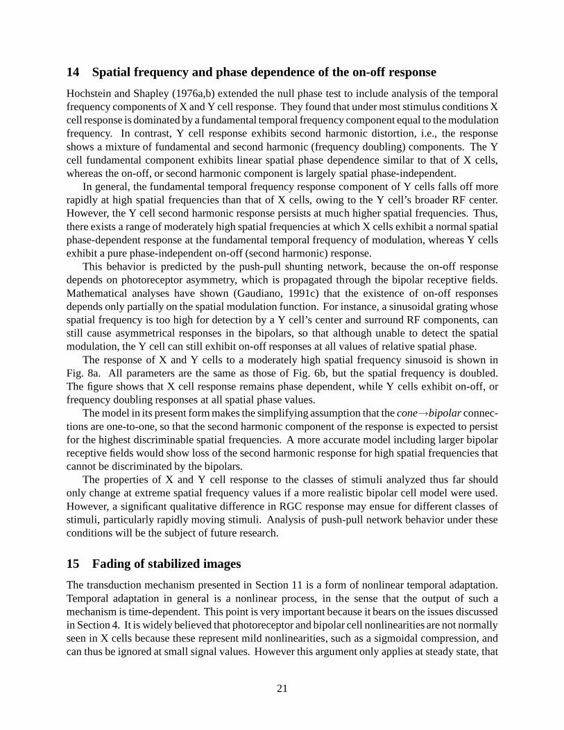
The response of X and Y cells to a moderately high spatial frequency sinusoid is shown inFig. 8a. All parameters are the same as those of Fig. 6b, but the spatial frequency is doubled.The figure shows that X cell response remains phase dependent, while Y cells exhibit on-off, orfrequency doubling responses at all spatial phase values.

The model in its present form makes the simplifying assumption that the cone!bipolar connec-tions are one-to-one, so that the second harmonic component of the response is expected to persistfor the highest discriminable spatial frequencies. A more accurate model including larger bipolarreceptive fields would show loss of the second harmonic response for high spatial frequencies thatcannot be discriminated by the bipolars.

The properties of X and Y cell response to the classes of stimuli analyzed thus far shouldonly change at extreme spatial frequency values if a more realistic bipolar cell model were used.However, a significant qualitative difference in RGC response may ensue for different classes ofstimuli, particularly rapidly moving stimuli. Analysis of push-pull network behavior under theseconditions will be the subject of future research.

15 Fading of stabilized images

The transduction mechanism presented in Section 11 is a form of nonlinear temporal adaptation.Temporal adaptation in general is a nonlinear process, in the sense that the output of such amechanism is time-dependent. This point is very important because it bears on the issues discussedin Section 4. It is widely believed that photoreceptor and bipolar cell nonlinearities are not normallyseen in X cells because these represent mild nonlinearities, such as a sigmoidal compression, andcan thus be ignored at small signal values. However this argument only applies at steady state, that

21

(a) (b)

Input

0o

270o

Y RGC Response

X RGC Response

L(x,t)

v(x,t)

v(x,t)

x

x

x

t

t

t

Photoreceptors

X ganglion cells

Luminance

L(x,t)

I(x,t)

v(x,t)

x

x

x

t

t

t

Figure 8: (a): Response of X and Y cell populations to a high spatial frequency grating thatis square-wave modulated in time. All parameters are the same as in Fig. 6b, but the spatialfrequency is doubled. (b): Responses of populations of photoreceptors and X cells to a sinusoidallymodulated grating. Responses fade quickly when the image is stabilized.

is, once the photoreceptors have had time to adapt. In order to suppress nonlinearities in responseto rapid temporal modulation, such as the square-wave modulation used by Enroth-Cugell andRobson (1966) and other authors, the photoreceptors would have to adapt instantaneously. Suchinstantaneous adaptation, aside from being unlikely in a biological setting, would lead to disastrouseffects: if each photoreceptor were able to instantly adjust its output range in response to inputfluctuations, then each photoreceptor would never be able to signal any temporal changes inluminance. Subsequent processing stages would then receive perfectly constant signals from allphotoreceptors, and would thus be functionally blind!

To clarify this point I will show that the simple photoreceptor adaptation law embodied inequations (21)-(22) predicts that the ratio of photoreceptor activations in response to two distinctillumination levels approaches unity as the photoreceptors approach equilibrium. In other words,stabilized images fade at the photoreceptors. To see this, consider two spatially distinct pointsin a visual scene, one of intensity L1, the other of intensity L2. Let the ratio of these signals be� = L1=L2. Denote the response of two photoreceptors exposed to these signals by I1 and I2. Ifboth photoreceptors have equilibrated to an initial signal L0 when the new pattern is presented,

22

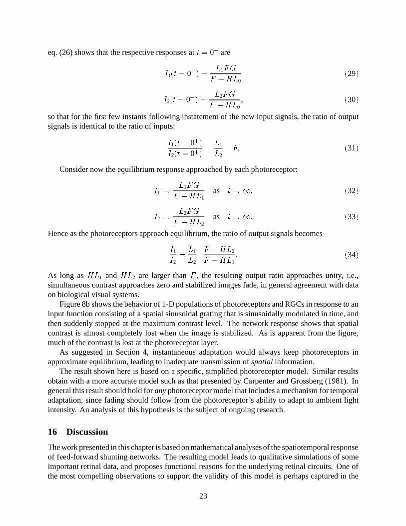
eq. (26) shows that the respective responses at t = 0+ areI1(t = 0+) = L1FGF +HL0(29)I2(t = 0+) = L2FGF +HL0

, (30)so that for the first few instants following instatement of the new input signals, the ratio of outputsignals is identical to the ratio of inputs:I1(t = 0+)I2(t = 0+) = L1L2

= �. (31)Consider now the equilibrium response approached by each photoreceptor:I1 ! L1FGF +HL1

as t!1, (32)I2 ! L2FGF +HL2as t!1. (33)

Hence as the photoreceptors approach equilibrium, the ratio of output signals becomesI1I2= L1L2

� F +HL2F +HL1. (34)

As long as HL1 and HL2 are larger than F , the resulting output ratio approaches unity, i.e.,simultaneous contrast approaches zero and stabilized images fade, in general agreement with dataon biological visual systems.

Figure 8b shows the behavior of 1-D populations of photoreceptors and RGCs in response to aninput function consisting of a spatial sinusoidal grating that is sinusoidally modulated in time, andthen suddenly stopped at the maximum contrast level. The network response shows that spatialcontrast is almost completely lost when the image is stabilized. As is apparent from the figure,much of the contrast is lost at the photoreceptor layer.

As suggested in Section 4, instantaneous adaptation would always keep photoreceptors inapproximate equilibrium, leading to inadequate transmission of spatial information.

The result shown here is based on a specific, simplified photoreceptor model. Similar resultsobtain with a more accurate model such as that presented by Carpenter and Grossberg (1981). Ingeneral this result should hold for any photoreceptor model that includes a mechanism for temporaladaptation, since fading should follow from the photoreceptor’s ability to adapt to ambient lightintensity. An analysis of this hypothesis is the subject of ongoing research.

16 Discussion

The work presented in this chapter is based on mathematical analyses of the spatiotemporal responseof feed-forward shunting networks. The resulting model leads to qualitative simulations of someimportant retinal data, and proposes functional reasons for the underlying retinal circuits. One ofthe most compelling observations to support the validity of this model is perhaps captured in the

23

paradoxical conclusion of Enroth-Cugell and Robson (1966) on the linearity of photoreceptors, aswas discussed in Section 4. The ability to adapt to ambient illumination without the undesirableside effects of nonlinear image processing has obvious ecological value. The push-pull shuntingnetwork overcomes this problem by combining two copies of the incoming signal in such a waythat the net input to the RGCs is always symmetrical about the average output level of a possiblynonlinear transducer, a property that can yield symmetrical null responses in X cells, and on-offresponses in Y cells. The results presented here also explain why X cells are less sensitive than Ycells to nonlinear input transients, but may sometimes exhibit on-off responses.

In addition to simulating and clarifying certain experimental findings on retinal ganglion cells,the model shows that adaptation laws of the form used here lead to loss of perceived contrast inresponse to sustained images. In other words, stabilized images fade. The relationship of thisfinding to the biologically observed fading of stabilized images is the subject of ongoing work.Such loss of contrast appears to be an inescapable side effect of temporal adaptation. Hence, just asthe original shunting network sacrifices temporal resolution in order to achieve spatial adaptation,so the photoreceptors sacrifice spatial resolution in order to achieve temporal adaptation.

Taken together with the results presented here, the above observations suggest that the retinaprovides an efficient means of maintaining high resolution in both space and time by sharing theload between three systems. The photoreceptors are able to optimize sensitivity in the temporaldomain by adjusting their dynamic range in response to changes in local luminance levels, butin doing so they lose much of their ability to process sustained spatial information. Conversely,the center-surround receptive field mechanism and shunting dynamics in the RGCs can extractuseful spatial information, but at least in some cases lead to degraded temporal resolution. Finally,the push-pull bipolar cells allow the RGCs to respond rapidly to increments and decrements of anonnegative input signal, and in so doing they ensure that spatial RGC processing is not affectedby photoreceptor nonlinearities.

The push-pull shunting network in its present form is a lumped model: no explicit equation isprovided for the behavior of the bipolar cells, and no mention is made of horizontal and amacrinecells. However, the lateral interactions that are lumped in the model’s equations must originate inhorizontal and amacrine cells. More accurate, quantitative data fits will require a more detailedphotoreceptor model, and an unlumped model of bipolar, horizontal and amacrine cells. This isparticularly important for simulations that examine spatial and temporal frequency response, as thephotoreceptor and bipolar cell response characteristics may be rate-limiting.

It is unclear at this time whether the transmitter gating law should be associated with photore-ceptor behavior as was done here. From a functional perspective, the temporal adaptation shouldoccur at the first stages of phototransduction. As indicated earlier, an enhanced version of this lawhas been used to model photoreceptor dynamics (Carpenter and Grossberg, 1981), and a heuristi-cally derived law of form (22) has been implicated in the transduction of light into neural signalsfor the vertebrate rod (Pugh and Lamb, 1990). However, the transient overshoots and undershootsobserved at and beyond the bipolar cell layer may be faster and more pronounced than those foundin the photoreceptors. In order to improve response time, the same type of gated transmission lawwith overall faster dynamics may thus also take place at synaptic junctions in the inner and outerplexiform layers. For example, in a related model Ogmen and Gagne (1990) have suggested thatthis type of transmitter dynamics may be found in the synaptic connection from photoreceptors tolarge monopolar cells in the fly.

The push-pull model can be used to make strong predictions about properties of amacrine and

24

horizontal cells, as well as bipolar cells. For example, if any portion of the RGC surround iscarried by amacrine cells, then it is expected that the amacrine cells must also receive push-pullbipolar inputs. Also, the ability to selectively discount sustained input components should onlyarise following the bipolar cell layer. This is one of the strongest predictions of the model, becausethe entire development of this work is based on the assumption that it is the push-pull action atthe bipolar level that allows the system to behave as a linear time-invariant system, and thus toinstantaneously disregard sustained input components even though light is a nonnegative physicalquantity. The model thus predicts that there should exist no classes of bipolar (or horizontal) cellsthat can give purely transient responses, a finding that receives some support in the experimentalliterature (e.g., chapter 4 of Dowling, 1987).

The existence of push-pull bipolar inputs to RGCs as proposed here receives some directexperimental support, though even this limited support has recently been questioned (Sterling,personal conversation). However, regardless of its validity as a model of specific retinal circuitry,the push-pull shunting network forces the conclusion that functional behavior of any cell cannotbe qualitatively inferred by the type and distribution of the inputs it receives. This is clearlydemonstrated by the X cell simulations in this chapter: the response of a simulated X cell appearslinear in spite of nonlinear preprocessing and nonlinear membrane properties of the X cell itself.

By the same token, the nature and distribution of input cells of different types cannot be inferredby observing RGC behavior. For example this model shows that the lack of on-off responses in Xcells does not preclude—but actually requires—the existence of inputs from both depolarizing andhyperpolarizing bipolar cells.

In light of these observations, I suggest that it is possible that push-pull bipolar inputs areubiquitous in the retina, but have not been reported because their existence is functionally elusive.

Note that a constraint similar to the one found for RGCs should also apply to other neuralprocessing stages. For instance, RGC output signals rely on axonal transmission (through actionpotentials) and are thus relegated to nonnegative values. Hence faithful spatiotemporal processingby cortical cells should require convergence of on-center and off-center RGCs. A similar mecha-nism has been suggested to explain the linearity of cortical simple cell responses in spite of floornonlinearities (e.g., thresholds) in RGC output (Emerson et al., 1987). The model presented inthis chapter extends that prediction by allowing for arbitrary preprocessing nonlinearities, and bysuggesting that the same mechanism may apply to other cortical cell classes.

There are still many insights to be gained from the mathematical form of the push-pull network.It is apparent that different choices of dynamical and morphological parameters can significantlyaffect model behavior. I should point out that although simulated X and Y cells were made to onlydiffer by a single parameter, this is obviously an oversimplification. For more accurate results thecenter and surround amplitudes (C and S), and the shunting saturation terms (B and D) shouldbe manipulated in conjunction with the RF center and surround widths (�C and �S ) to achievea desired functional behavior. The single-parameter change is meant to emphasize the ability toaffect RGC function by means of simple parametric changes within a single formal model.

Another unique aspect of this model is that it was not originally derived to simulate RGC data,but was instead formulated as a means of simultaneously achieving accurate spatial and temporalprocessing in feed forward shunting networks. This is a complementary approach to models thatare grounded in experimental data, and often designed to reproduce retinal behavior by joiningmany detailed models of each element or layer of the retina (e.g., Rodieck, 1965; Siminoff, 1991;Sterling et al., 1987; Werblin, 1991). While the present model purports to explain the reason for

25

adopting a certain architecture, the experimentally derived models contain very important data onmany anatomical, physiological, and pharmacological properties of individual cells in the retina.Future research combining the push-pull architecture and details from such experimental modelswill undoubtedly yield more accurate results and a clearer understanding of retinal function.

References

Barlow, H.B. (1953). Summation and inhibition in the frog retina. Journal of Physiology, 119: 69–88.

Boycott, B.B. and Wassle, H. (1974). The morphological types of ganglion cells of the domestic cat’s retina.Journal of Physiology, 240: 397–419.

Bullock, D. and Grossberg, S. (1988). Neural dynamics of planned arm movements: Emergent invariantsand speed-accuracy properties during trajectory formation. Psychological Review, 95, 49-90.

Carpenter, G.A. and Grossberg, S. (1981). Adaptation and trasnsmitter gating in vertebrate photoreceptors.Journal of Theoretical Neurobiology, 1: 1-42.

Cleland, B.G. and Levick, W.R. (1974). Brisk and sluggish concentrically organized ganglion cells in thecat’s retina. Journal of Physiology, 240: 421–456.

Ditchburn, R.W., and Ginsborg, B.L. (1952). Vision with a stabilized retinal image. Nature, 170, 36–37.

Dowling, J.E. (1987). The retina: an approachable part of the brain. Belknap: Cambridge, USA.

Emerson, R.C. Korenberg, M.J., and Citron, M.C. (1989). Identification of intensive nonlinearities incascade models of visual cortex and its relation to cell classification. In Marmarelis, V.Z. (Ed.) Advancedmethods of physiological system modeling. New York: Plenum Press.

Enroth-Cugell, C. and Robson, J.G. (1966). The contrast sensitivity of retinal ganglion cells of the cat.Journal of Physiology, 187: 517–552.

Freed, M.A. and Sterling, P. (1988). The ON-alpha ganglion cell of the cat retina and its presynaptic celltypes. Journal of Neuroscience, 8 (7): 2303–2320.

Fukuda, Y., Hsiao, C.-F., Watanabe, M., and Ito, H. (1984). Morphological correlates of physiologicallyidentified Y, X and W cells in the cat retina. Journal of Neurophysiology, 52: 999–1013.

Furman, G.G. (1965). Comparison of models for subtractive and shunting lateral-inhibition in receptor-neuron fields. Kybernetyk, 2: 257–274.

Gaudiano, P. (1991a). Neural network models for spatio-temporal visual processing and adaptive sensory-motor control. Unpublished doctoral dissertation, Boston University.

Gaudiano, P. (1991b). A Unified Neural Network Model of Spatio-Temporal Processing in X and Y RetinalGanglion Cells. I: Analytical Results. Biological Cybernetics, in press (1992).

Gaudiano, P. (1991c). A Unified Neural Network Model of Spatio-Temporal Processing in X and Y RetinalGanglion Cells. II: Temporal Adaptation and Simulation of Experimental Data. Biological Cybernetics,in press (1992).

Grossberg, S. (1968). Some physiological and biochemical consequences of psychological postulates.Proceedings of the National Academy of Sciences, 60: 758–765.

Grossberg, S. (1970). Neural Pattern Discrimination. Journal of Theoretical Biology, 27: 291–337.

Grossberg, S. (1973). Contour enhancement, short-term memory, and constancies in reverberating neuralnetworks. Studies in Applied Mathematics, 52: 217-257.

26

Grossberg, S. (1980). Intracellular mechanisms of adaptation and self-regulation in self-organizing networks:the role of chemical transducers. Bulletin of Mathematical Biology, 42: 365–396.

Grossberg, S. (1983). The quantized geometry of visual space: The coherent computation of depth, form,and lightness. Behavioral and Brain Sciences, 6: 625–692.

Grossberg, S. (1988). Nonlinear neural networks: Principles, mechanisms, and architectures. Neural Net-works, 1: 17-61.

Hochstein, S. and Shapley, R.M. (1976a). Quantitative analysis of retinal ganglion cell classifications.Journal of Physiology, 262: 237–264.

Hochstein, S. and Shapley, R.M. (1976b). Linear and nonlinear spatial subunits in Y cat retinal ganglioncells. Journal of Physiology, 262: 265–284.

Hodgkin, A.L. (1964). The conduction of the nervous impulse. Liverpool: Liverpool University Press.

Kolb, H., Nelson, R. and Mariani, A. (1981). Amacrine cells, bipolar cells and ganglion cells of the catretina: a Golgi study. Vision Research, 21: 1081–1114.

Kuffler, S.W. (1953). Discharge patterns and functional organization of the mammalian retina. Journal ofPhysiology, 16: 37–68.

McGuire, B.A., Stevens, J.K., and Sterling, P. (1986). Microrcircuitry of beta ganglion cells in cat retina.Journal of Neuroscience, 6: 907–918.

Ogmen, H., and Gagne, S. (1990). Neural models for sustained and ON-OFF units of insect lamina.Biological Cybernetics, 63: 51–60.

Pugh, E.N. Jr, and Lamb, T.D. (1990). Cyclic GMP and calcium: the internal messenger of excitation andadaptation in vertebrate photoreceptors. Vision Research, 30 (12): 1923–1948.

Rodieck, R.W. (1965). Quantitative analysis of cat retinal ganglion cell response to visual stimuli. VisionResearch, 5, 583–601.

Saito, H. (1983). Morphology of physiologically identified X-, Y- and W-type retinal ganglion cells of thecat. Journal of Comparative Neurology, 221: 279–288.

Schiller, P. (1982). Central connections of the retinal On and Off pathways. Nature, 297: 580–583.

Slaughter, M.M, and Miller, R.F. (1982). 2-Amino-4-phosphonobutyric acid: a new pharmacological toolfor retina research. Science, 211, 182–185.

Sperling, G. (1970). Model of visual adaptation and contrast detection. Perc. & Psychophys., 8 (3): 143–157.

Sperling, G. and Sondhi, M.M. (1968). Model for visual luminance discrimination and flicker detection.Journal of the Optical Society of America, 58: 1133–1145.

Sterling, P. (1990). Retina. In Shepherd, G.M. (Ed.) The synaptic organization of the brain. New York:Oxford University Press, third edition. Chapter 6, 170–213.

Werblin, F. (1971). Adaptation in a vertebrate retina: Intracellular recordings in Necturus. Journal ofNeurophysiology, 34: 228–241.

Werblin, F. (1991). Synaptic connections, receptive fields, and patterns of activity in the tiger slamanderretina. Investigative Ophthalmology and Visual Science, 32 (3), 459–483.

Werblin, F. and Dowling, J.E. (1969). Organization of the retina of the mudpuppy, Necturus maculosus. II.Intracellular recording. Journal of Neurophysiology, 32: 339–355.

27