GA–A23542

TOWARD A FULL-RADIUS CONTINUUMGYROKINETIC SIMULATION CODE

byJ. CANDY, R.E. WALTZ, and M.N. ROSENBLUTH

OCTOBER 2000

This report was prepared as an account of work sponsored by an agencyof the United States Government. Neither the United States Governmentnor any agency thereof, nor any of their employees, makes any warranty,express or implied, or assumes any legal liability or responsibility for theaccuracy, completeness, or usefulness of any information, apparatus,product, or process disclosed, or represents that its use would not infringeupon privately owned rights. Reference herein to any specific commercialproduct, process, or service by trade name, trademark, manufacturer, orotherwise, does not necessarily constitute or imply its endorsement,recommendation, or favoring by the United States Government or anyagency thereof. The views and opinions of authors expressed herein donot necessarily state or reflect those of the United States Government orany agency thereof.

GA–A23542

TOWARD A FULL-RADIUS CONTINUUMGYROKINETIC SIMULATION CODE

byJ. CANDY, R.E. WALTZ, and M.N. ROSENBLUTH

This is a preprint of a paper presented at the Joint Varenna-Lausanne International Workshop, August 28–September 1,2000, Varenna, Italy, and to be printed in the Proceedings.

Work supported byU.S. Department of Energy

Grant No. DE-FG03-95ER54309

GENERAL ATOMICS PROJECT 3726OCTOBER 2000

Toward a full-radius continuum gyrokineticsimulation code

J. Candy, R.E. Waltz and M.N. RosenbluthGeneral Atomics, San Diego, CA

May 30, 2001

Abstract

In this paper we detail some first results from the continuum gyrokineticmicroturbulence code, gyro. In addition to standard ITG (ion temperaturegradient) and adiabatic electron physics, gyro includes trapped and passingelectrons with electromagnetic effects in real geometry. These features are incommon with the gs2 code [1]. The novel feature of gyro is the use of a radialgrid rather than a grid in kr = −i ∂/∂r. The real-space grid allows gyro toinclude profile variation effects. When operated with periodic radial boundaryconditions in the vanishing-ρ∗ flux-tube limit, gyro is designed to reproducegs2 results (obtained using a ballooning-mode formalism). gyro results atfinite-ρ∗ (i.e. profile variation) will be reported in future work. To date we havecomplete agreement with finite-β comparisons to the linear gks code [2], andhave also verified the Rosenbluth-Hinton linear decrement of the n=0 zonalflows [3].

1 Introduction

The Gyrokinetic-Maxwell (GKM) equations lay a firm but computationally challeng-ing foundation for the investigation of microinstabilities and anomalous transport infusion plasmas. To this end, we began development of gyro – a nonlinear, electro-magnetic, finite-β gyrokinetic code that incorporates a grid representative of real toka-mak geometry. Eventually, gyro will contain all physics of low-frequency (ω < ωci)plasma turbulence, assuming only that the ion gyroradius is less than the magneticfield gradient length. The decision to pursue a full-radius code was made in orderto (i) quantify avalanches and action-at-a-distance effects; (ii) describe finite-ρ∗ dia-magnetic velocity shear stabilization of turbulence, where ρ∗ ≡ ρ/a; and (iii) captureenough physics so that comparison of thermal diffusivities obtained from simulationcan be directly compared with experiment.

1

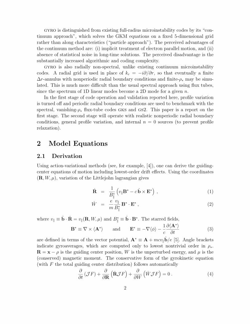
gyro is distinguished from existing full-radius microinstability codes by its “con-tinuum approach”, which solves the GKM equations on a fixed 5-dimensional gridrather than along characteristics (“particle approach”). The perceived advantages ofthe continuum method are: (i) implicit treatment of electron parallel motion, and (ii)absence of statistical noise in long-time solutions. The perceived disadvantage is thesubstantially increased algorithmic and coding complexity.

gyro is also radially non-spectral, unlike existing continuum microinstabilitycodes. A radial grid is used in place of kr = −i∂/∂r, so that eventually a finite∆r-annulus with nonperiodic radial boundary conditions and finite-ρ∗ may be simu-lated. This is much more difficult than the usual spectral approach using flux tubes,since the spectrum of 1D linear modes become a 2D mode for a given n.

In the first stage of code operation and validation reported here, profile variationis turned off and periodic radial boundary conditions are used to benchmark with thespectral, vanishing-ρ∗ flux-tube codes gks and gs2. This paper is a report on thefirst stage. The second stage will operate with realistic nonperiodic radial boundaryconditions, general profile variation, and internal n = 0 sources (to prevent profilerelaxation).

2 Model Equations

2.1 Derivation

Using action-variational methods (see, for example, [4]), one can derive the guiding-center equations of motion including lowest-order drift effects. Using the coordinates(R,W, µ), variation of the Littlejohn lagrangian gives

R =1

B∗‖

(v‖B

∗ − c b× E∗), (1)

W =e

m

v‖B∗‖

B∗ · E∗ , (2)

where v‖ ≡ b · R = v‖(R,W, µ) and B∗‖ ≡ b ·B∗. The starred fields,

B∗ ≡ ∇× 〈A∗〉 and E∗ ≡ −∇〈φ〉 − 1

c

∂〈A∗〉∂t

(3)

are defined in terms of the vector potential, A∗ ≡ A + mcv‖b/e [5]. Angle bracketsindicate gyroaverages, which are computed only to lowest nontrivial order in ρ∗.R = x− ρ is the guiding center position, W is the unperturbed energy, and µ is the(conserved) magnetic moment. The conservative form of the gyrokinetic equation(with F the total guiding center distribution) follows automatically

∂

∂t(JF ) +

∂

∂R

(RJF

)+

∂

∂W

(WJF

)= 0 . (4)

2

In Eq. (4), we have introduced the velocity-space Jacobian J ≡ (v/v‖)B∗‖ . In the

equations of motion, no explicit separation into equilibrium and perturbed quanti-ties fields has been made. To derive the GKM equations for low-β electromagneticperturbations, it is simplest if we proceed by considering a class of vector potentialsA = A0 + A‖b. Here, b is the unit vector along the perturbed field, B0 = ∇×A0 isthe equilibrium magnetic field, and the corresponding perturbed B-field is

δB = ∇A‖ × b + A‖∇× b ∇A‖ × b +A‖B

b×∇B (5)

where the approximate equality is valid in the limit of low-β, with the implicationthat the magnetic perturbation satisfies b · δB = 0. This means that the componentof perturbation parallel to the equilibrium field is negligibly small. Additionally,according to the gyrokinetic ordering [6], the second term in Eq. (5) is smaller thanthe first. It is therefore ignored, as are terms containing ∂b/∂t. Henceforth, weconsider only 〈φ〉 and 〈A‖〉 to be perturbed quantities (with b now taken alongthe equilibrium field). Then, we have

∂F

∂t+ vg ·

∂F

∂R− e

m

(vg · ∇〈φ〉+

v‖c

∂〈A‖〉∂t

)∂F

∂W= 0 (6)

where vg ≡ v‖b + vd + vE + (v‖/B)∇〈A‖〉 × b, with

vd ≡v2‖ + µB

B2b×∇B and vE ≡

c

Bb×∇〈φ〉 (7)

Now, split F into F = F0 +f , where F0 represents the macroscopic equilibrium whichchanges on the transport timescale, and f represents microscopic fluctuations whichare smaller by one order in ρ∗. Also, ignore all nonlinearities connected with the thirdterm on the LHS of (6), which are similarly small by one order in ρ∗. One can showthat the equation describing microscopic fluctuations (for each species) is

∂g

∂t+ (v‖b + vd) ·

∂g

∂R= −∂F0

∂W

∂〈U〉∂t− 1

Bb×∇〈U〉 · ∇(F0 + g) (8)

where

f = 〈φ〉 ∂F0

∂W+ g and U ≡ φ− v‖A‖ . (9)

Eq. (8) is the form of the gyrokinetic equation solved by gyro, and is equivalentto that originally derived by Frieman and Chen [6]. Note that for electrons, thegyroaverage is treated as the identity operation. The field evolution is subsequentlydetermined by a sum over all species (subscript s) in the gyro-Maxwell equations:

−∇2φ(x, t) = 4π∑s

ezs

∫d3v

(zseφ(x)

∂F0s

∂W+ 〈g〉s

), (10)

−∇2A‖(x, t) = 4π∑s

ezs

∫d3v v‖〈g〉s . (11)

3

In Eqs. (10) and (11), all functions including 〈g〉 are evaluated at the plasma positionx. These equations are consistent to lowest nontrivial order in ρ∗ with the work ofHahm [7].

2.2 Coordinate system

gyro uses a real-space coordinate system (r, θ, α), where r is a flux-surface label(b · ∇r = 0), and θ is an angle in the poloidal plane. The toroidal coordinate

α ≡ ζ −∫ θ

0dθ q , (12)

with q ≡ (b · ∇ζ)/(b · ∇θ) the local safety factor, is chosen to be constant alonga field line (b · ∇α = 0). The parallel derivative in these coordinates is simplyb · ∇ = (b · ∇θ)∂θ. In this article, the bare symbol q is reserved for the flux-surface-averaged safety factor.

q ≡ 1

2π

∫ 2π

0dθ q (13)

2.3 Representation of Perturbed Quantities

We expand (φ,A‖, g) as Fourier series in α. For example, the electrostatic potentialis written

φ =∑n

φn(r, θ)e−inα (14)

Although the physical field, φ, is 2π-periodic in θ, this representation has the implica-tion that the Fourier coefficients, φn, are nonperiodic, and satisfy the phase conditionφn(r, π) = φn(r,−π) exp[−2πinq(r)]. Since φ is real, the coefficients satisfy φ∗n = φ−n.

2.4 Normalization

Our choice of units is summarized in Table. 1. Beyond this, we introduce renormalizeddensities and distribution functions ns and gs according to ns = nsne(0) and gs =gsne(0)FM

s , respectively, Here, FMs ≡ e−W/Ts/(π3/2v3

s ) and Ts(r) = msv2s /2. The

equilibrium distribution is just F0s = ns FMs

The velocity integrals in Eqs. (10) and (11) are rewritten in terms of the energy, W ,and pitch angle, λ ≡ µ/W , using the identity

∑σ(2π) dW dλ = (m2v‖/B) d3v , where

σ ≡ sgn(v‖). Then for each species we introduce the operator V , such that

∫d3v FMf =

∑σ

V σ[fσ] with V σ[f ] ≡ 1

2√π

∫ ∞0

dε e−ε√ε

∫ 1

0

d(λB)fσ√1− λB

, (15)

and ε ≡ W/T . It can be verified that∑σ V

σ[1] = 1.

4

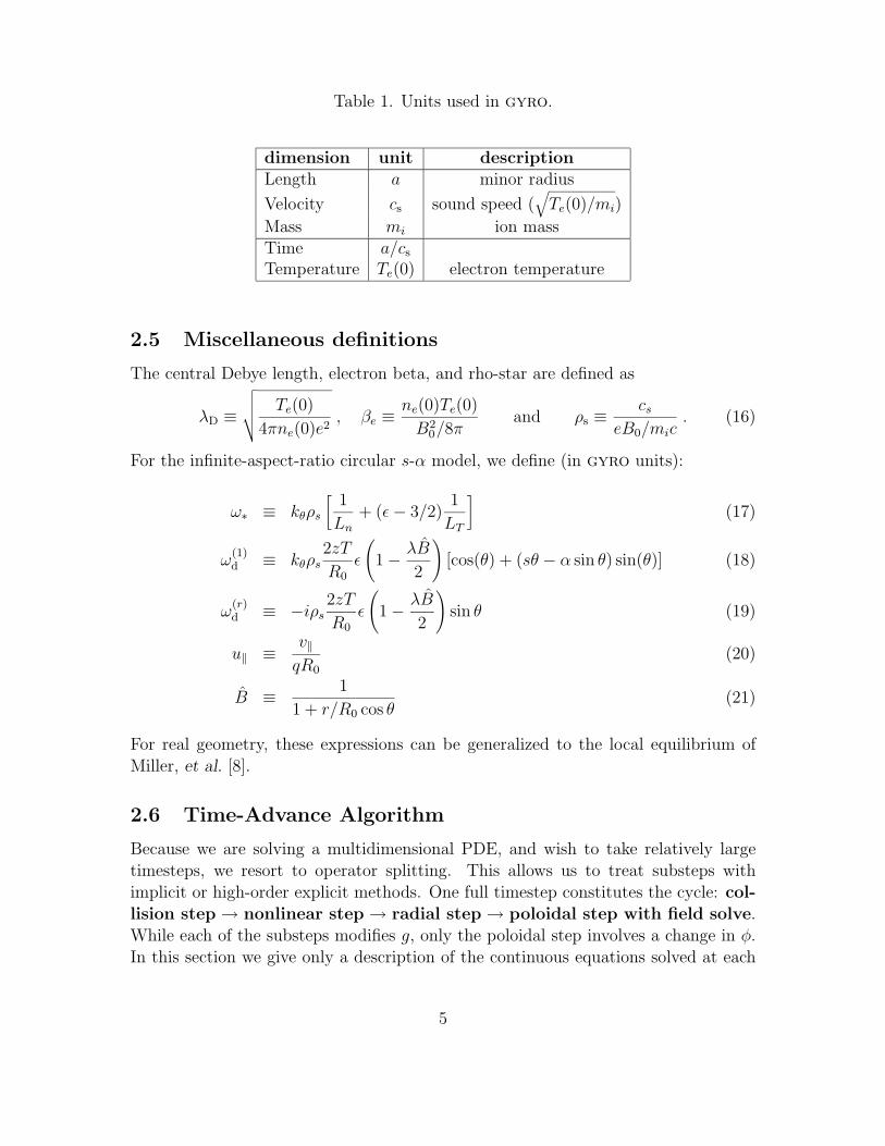
Table 1. Units used in gyro.

dimension unit descriptionLength a minor radius

Velocity cs sound speed (√Te(0)/mi)

Mass mi ion massTime a/cs

Temperature Te(0) electron temperature

2.5 Miscellaneous definitions

The central Debye length, electron beta, and rho-star are defined as

λD ≡√√√√ Te(0)

4πne(0)e2, βe ≡

ne(0)Te(0)

B20/8π

and ρs ≡cs

eB0/mic. (16)

For the infinite-aspect-ratio circular s-α model, we define (in gyro units):

ω∗ ≡ kθρs

[1

Ln+ (ε− 3/2)

1

LT

](17)

ω(1)d ≡ kθρs

2zT

R0

ε

(1− λB

2

)[cos(θ) + (sθ − α sin θ) sin(θ)] (18)

ω(r)d ≡ −iρs

2zT

R0

ε

(1− λB

2

)sin θ (19)

u‖ ≡v‖qR0

(20)

B ≡ 1

1 + r/R0 cos θ(21)

For real geometry, these expressions can be generalized to the local equilibrium ofMiller, et al. [8].

2.6 Time-Advance Algorithm

Because we are solving a multidimensional PDE, and wish to take relatively largetimesteps, we resort to operator splitting. This allows us to treat substeps withimplicit or high-order explicit methods. One full timestep constitutes the cycle: col-lision step → nonlinear step → radial step → poloidal step with field solve.While each of the substeps modifies g, only the poloidal step involves a change in φ.In this section we give only a description of the continuous equations solved at each

5

substep. The collision step, which solves for the response due to pitch-angle scat-tering, is not discussed for the sake of brevity. Moreover, the length of the presentpaper allows only an outline of the numerical methods, discretized equations andparallelization algorithms used in gyro.

Nonlinear Step Here we make a partial advance using the nonlinear terms only, andadapt the method of advance accordingly. In the ballooning limit, and for circularflux surface, the continuous equation to be solved (for each GKE species) can bewritten as

∂tgn =iρsq

r

∑n′

[n〈U〉n′∂rgn−n′ − n′∂r

(gn′〈U〉n−n′

)](22)

The discretization scheme, to a very good approximation, is designed to satisfy thefollowing entropic conservation law:

∂

∂t

∫dα

∫dr |g|2 → ∂

∂t

∑n

∫dr |gn|2 ∼ O(∆t4) (23)

Using centered finite differences in r, we emphasize that use of the conservative formgiven in Eq. (22) is essential to obtain the result of Eq. (23). In practice, at leastfive-point (fourth-order) rules are required. The system of ordinary equations is thenadvanced in time using a fourth-order explicit Runge-Kutta method. The result isthat the change in entropy in one nonlinear step is O(∆t)5.

Radial Step The radial step ignores all but radial derivatives contained in the linearterms. Physically, this accounts for the physics connected with the radial derivative,ω

(r)d ∂r, in the curvature drift, ωd = ω

(1)d + ω

(r)d ∂r

∂tg = iω(r)d ∂rg (24)

In the simplest case where ω(r)d is held fixed at the central radius (i.e., the ballooning

limit), we can solve the equation exactly on a given radial grid at the expense of aforward and backward Fourier transform. This method has the added benefit that atno extra expense we can add hyperviscosity to eliminate the effects of electron Landauresonances in the electron kinetic equation. Banded-diagonal solvers are used in thenonperiodic case where radial variation is accounted for.

Poloidal Step The poloidal step ignores derivatives with respect to pitch angle,energy and radius. Nonlinearities are also neglected. We use a phase-space conserv-ing differencing scheme to avoid passing-particle instability of n = 0 modes. Thenormalized equations are(

∂t + u‖∂θ)g = α∂t〈U〉+ iω

(1)d g − inω∗〈U〉 , (25)

λ2D∇2φ +

∑s

zs

∑σ

V σ[〈g〉σs ] +∑s

zsαsφ = 0 (26)

6

2ρ2s

βe∇2A‖ +

∑s

zs

∑σ

V σ[v‖〈g〉σs ] = 0 , (27)

with α ≡ zn/T . These equations are solved implicitly for both electrons and ionsto yield a partial advance of g and (φ,A‖). We remark that an implicit field-solve isessential for the electron equations to avoid the Courant limit on timestep imposedby the parallel operator

(∂t + u‖∂θ

)g.

with α ≡ zn/T . These equations are solved implicitly for both electrons and ionsto yield a partial advance of g and (φ,A‖). We remark that an implicit field-solve isessential for the electron equations to avoid the Courant limit on timestep imposedby the parallel operator

(∂t + u‖∂θ

)g.

2.7 Radial Grid Specification

For a given choice of equilibrium and reference mode number nref , ballooning modesoscillates at wavelengths kr = (p + ./.∗)k∗, where k∗ ≡ 2πskref

θ and krefθ = nrefq/r.

A given mode has a fixed integer values of ., with 0 ≤ . < .∗, and runs over allintegral values of p. The most unstable mode has . = 0, and more stable modes. > 0. Knowing k∗ and .∗, we set the box length at L = 2π.∗/k∗. Numerically, weretain only a finite number of p-values for each mode (|p| ≤ j∗), since the partialcontribution to the eigenmode drops off rapidly with each successive p. Then, thenumber of radial gridpoints required to describe .∗ ballooning modes at n = nref isnr = 2j∗.∗ + 1.

A value for ρs is also required – typically, we choose krefθ ρs ∼ 0.3. Experience

shows that for s ∼ 1, it is generally sufficient to choose five k’s per ballooning mode(j∗ = 2), or equivalently nr = 4.∗ + 1, where nr is the number of radial gridpoints.A linear calculation of only the most unstable mode requires .∗ = 1. Nonlinear runstypically require .∗ = 24 (and at least ten values of n) for proper saturation. A crucialfeature of the code is that the code timing and storage increase linearly with nr. Thisis a result of banding methods which make use of the localized nature of gyroaveragesand derivatives in a realistic simulation box.

2.8 Numerical problems

We have encountered a number of subtle numerical difficulties associated with thereal-space grid used in gyro. The most troublesome of these was connected withn = 0 field-solve matrix – used in the poloidal step. This matrix has a null eigenvaluefor kr = 0. Although we do not evolve the equilibrium (kr = 0, n = 0), the smallestvalues of kr used in nonlinear simulations are prone to numerical instability whichappears as a result of the split radial and poloidal steps. We have cured this instabilityusing (i) a conservative differencing scheme for Eq. (25) together with (ii) a two-stage

7

(predictor-corrector type) method to improve the accuracy of the total linear step(radial plus poloidal). This ensures to high accuracy the balance between the terms

iω(r)d ∂rg and u‖∂θg for n = 0.

3 Numerical Results

To benchmark gyro for finite-n ballooning modes, it is convenient to use the linearelectromagnetic solver gks [2]. The validity and accuracy of gks have been rigor-ously established. The simulation results presented generally share a common set ofinput parameter values, as summarized in Table 2. When exceptions occur, they areindicated. In Table 2, nε is the number of energy gridpoints, nλ is the number of pitchangle gridpoints, and nθ is the number of gridpoints in poloidal angle. Because wemultipoint methods for radial integration and differentiation, we obtain much higherthan second order accuracy.

Table 2Nominal parameter values for the simulations presented in this paper.

Exceptions are indicated as needed.

parameter value parameter value parameter valueR/a 3.0 r/a 0.5 a/LT 3.0a/LN 1.0 s 1.0 q 2.0nε 5 nλ 26 nθ 32

3.1 Electrostatic adiabatic electron case

For this test, we perform one gyro run with a fine radial grid (nr = 97) and 15toroidal modes (n = 0, 5, 10, . . . , 70). Electrons are held adiabatic. The correspondingky-spectrum is kθρs = 0.0, 0.05, 0.1, . . . , 0.7. The results, shown in Fig. 1, are inagreement with gks.

3.2 Electromagnetic ballooning modes

Although gyro is not a ballooning code (that is, the equations and associated bound-ary conditions are not functions of a ballooning angle), it is possible to reconstruct anequivalent (or nearly equivalent) ballooning-space solution from the real-space gyro

solution. In gyro, the largest kr is damped to mimic the gks boundary condition,which accurately eliminates the small, fine-scale electron Landau layer response.

To obtain an electromagnetic response, we choose βe = 0.004 (note that βcrit =0.055) and kθρs = 0.3. Here we use only enough radial gridpoints (nr = 5) to capture

8

the most unstable mode (.∗ = 1, j∗ = 2, kr = pk∗, p = −2, . . . , 2). gyro findsa frequency (a/cs)(γ, ω) = (0.167,−0.361) versus (0.175,−0.357) from gks. Whenplotted as a function of ballooning angle, as in Fig. 2, the results are essentially thesame as one would obtain from a ballooning code. In addition, going to nr = 97 atthe same radial grid spacing gives the same complex eigenfrequency.

3.3 Electrostatic nonadiabatic electron parameter scan

Now, we try the linear electromagnetic case again, but with the full nonlinear radialgrid (nr = 97) and nn = 15 (kθρs as in Sec. 3.1). The box length, L = 80ρs, is alsothat which is used in nonlinear runs. The results, shown in Fig. 3, compare well withgks runs on case-dependent grids.

3.4 Axisymmetric modes

Keeping the parameters the same as in the previous section, but setting n = 0 (or,equivalently, kθ = 0), we can test the accuracy of axisymmetric poloidal flow decay.That linear collisionless processes do not damp these flows was clearly shown byRosenbluth and Hinton [3]. Their work also gave a prediction for the level of residualflow to be expected. This prediction is completely consistent with gyro results, asillustrated in Fig. 4.

3.5 Nonlinear ITG

By turning on the nonlinear interaction, Eq. (22), we can make runs to determine, forexample, the turbulent thermal diffusivity in the simulation domain. For a benchmarkrun, we set the grid resolution at nr = 97, L = 80ρs, nθ = 16, nλ = 14, nn = 14,kθρs = 0, 0.06, . . . , 0.78 and (cs/a)∆t = 0.05 (with other parameters as in Table 1).Results are shown in Figs. 5 to 9. The overall level of thermal diffusivity (Fig. 5) χi ∼3.25 is comparable with the gs2 value of 4.0 (B. Dorland, private communication).An explanation of the possible sources of this minor discrepancy is a complicatedmatter, and is the subject of ongoing investigation.

A visual illustration of the onset of turbulence given in a sequence of poloidal cross-section plots. Fig. 7 shows radially elongated linear structures (ballooning modes) at(cs/a)t = 50. During this early time, the linear modes are only weakly deformed bythe self-generated n = 0 flow. In Fig. 8, by (cs/a)t = 90, the deformation has becomestronger and is nearing the point where linear modes are sheared apart radially.Finally, in Fig. 9 we show the density fluctuations in the early turbulent stage at(cs/a)t = 300.

9

3.6 Code performance

A domain decomposition algorithm has been devised to deal with the communicationrequirements set by operator splitting, and to minimize as much as possible commu-nication (message-passing) bandwidth limitations. The code in its present form scaleswell up to the current capacity (512 processors) of both the NERSC IBM RS/6000SP and CRAY T3E-900 machines, with slightly higher maximum performance on theIBM. gyro also performs well on the General Atomics Intel Beowulf clusters. Inparticular, the maximum performance on the larger stella cluster averages about1/10th that of the full IBM SP. Quantitative results are given in Fig. 10.

4 Progress and Conclusions

Through a series of numerical benchmarks with existing codes, we have demonstratedthat gyro operates correctly and efficiently in flux-tube mode, while carrying withit the heavy infrastructure required for full-radius operation. In particular, the use ofbanded multi-point methods for gyroaverages, nonlinear derivatives and field-solvesallows linear-in-nr code scaling. Comparisons with gks for the eigenvalues of linear,electromagnetic n > 0 ballooning modes show very good agreement, especially con-sidering differences in boundary conditions. We also find that n = 0 modes behavein accordance with Rosenbluth-Hinton theory [3]. Results from nonlinear simulationsare in rough preliminary agreement with gs2.

5 Acknowledgements

This is a report of work supported by the U.S. Department of Energy under GrantNo. DE-FG03-95ER54309 and the Advanced Computing Initiative.

References

[1] F. Jenko, W. Dorland, M. Kotschenreuther and B.N. Rogers, Phys. Plasmas 7(2000) 1904. Fluids 25 (1982) 502.

[2] M. Kotschenreuther, et al., Comput. Phys. Commun., 88 (1995) 128.

[3] M.N. Rosenbluth and F.L. Hinton, Phys. Rev. Lett. 80 (1998) 724.

[4] R.G. Littlejohn, J. Plasma Phys., 29 (1983) 111.

[5] Morozov, A.I. and Solov’ev, L.S., Reviews of Plasma Physics (Plenum, ed. M.A.Leontovich), vol. 2 (1966) 201.

[6] E.A. Frieman and L. Chen, Phys. Fluids 25 (1982) 502.

[7] T.S. Hahm, Phys. Fluids 31 (1988) 2670; T.S. Hahm, Phys. Plasmas 3 (1996)4658.

10

[8] R.L. Miller, M.S. Chu, J.M. Greene, Y.R. Lin-Liu, and R.E. Waltz, Phys. Plas-mas 5 (1988) 973; R.E. Waltz and R.L. Miller, Phys. Plasmas 6 (1999) 4265.

11

12

0.150.00

0.00 0.10 0.20 0.30 0.40 0.50 0.60

–0.10

–0.20

–0.30

–0.40

–0.50

–0.60

0.10

GYROGKSGYRO

(a) (b)

GKS

0.05

0.000.00 0.10 0.20 0.30

kθρskθρs

(a/c

s)γLI

NEAR

(a/c

s)ωLI

NEAR

0.40 0.50 0.60

Fig 1. Frequency (left) and growth rate (right) comparison for electrostaticmodes with adiabatic electrons. Solid lines show GKS values.

0.041.0

0.5

–0.5

–1.0

0.0

0.02

–0.02

–0.04

–4 –2 0

θ*/π2 4–4

(a) (b)

–2 0

θ*/π2 4

A ll(θ*)

φ(θ *)

0.00

Fig 2. Electrostatic and vector potentials, φ and A || , as functions of theballooning angle, θ* = θ + 2πp. Note that p is defined in Sec. 2.7.

13

0.30

0.5

0.0

–0.5

GYROGKS

GYROGKS

0.25

0.20

0.15

0.10

0.05

0.000.0 0.2

kθρs

0.4 0.6 0.80.0 0.2kθρs

0.4 0.6 0.8

ITG regionITG region TEM regionTEM region

(a/c

s)γLI

NEAR

(a/c

s)ωLI

NEAR

(a) (b)

Fig. 3. Frequency and growth rate comparison for nonadiabatic electron case.Solid lines are GKS values.

1.0 0.50

0.40

0.30

0.20

0.10

0.000 5 10 15 20

GAM period

RH theoryGYRO

RH theory: 1/(1+x)

GYRO (q=1, R/r=6)GYRO (q=1, R/r=12)GYRO (q=1.4, R/r=5)GYRO (q=2, R/r=6)

0.8

0.6

0.4

0.2

0.00 50 100

(cs/a) t150 200

⟨φ(t)

⟩ RMS/⟨φ

(0)⟩ RM

S

RH re

sidu

al

x = 1.6q2(R/r)0.5

(a) (b)

Fig. 4. Axisymmetric poloidal flow dynamics. Left plot shows GYRO dynamicresponse (solid line) decay to Rosenbluth-Hinton theoretical residual. Right plotshows computed versus theoretical residuals for four separate runs.

14

(a) (b)0.04

RMS

fluct

uatio

ns 0.03

0.02

0.01

0.000 200

(cs/a) t400 600 8000

0

1

2

3

4

5

200

Average χi = 3.25

χ i [un

its o

f (c s

/a)ρ

s2 ]

RMS variation in χi = 0.48

(cs/a) t

400 600 800

⟨φ(n≠0)⟩RMS⟨φ(n=0)⟩RMS

Fig. 5. Thermal diffusivity (left). Evolution of the electrostatic potential, φ ,showing separation between the axisymmetric n = 0 and nonaxisymmetric n ≠ 0components (right).

⟨φ(n,ρ)⟩RMS [a.u.]1.00

0.10

0.0160

4020

–20–40–60

0

020

40 n60

80

ρ

Fig. 6. RMS time-averaged spectral content ( kr = pkmin,n) of the turbulentpotential. Note the logarithmic scale.

15

0.6

0.4

0.2

0.0

–0.2

–0.4

–0.6–0.6 –0.4 –0.2 0.0 0.2

x/a

Z/a

0.4 0.6

Fig. 7. Density fluctuations, δne(r,θ ) in the poloidal cross-section ϕ = 0 . Thedynamics, shown here at (cs / a)t = 50 are still dominantly linear.

0.6

0.4

0.2

0.0

–0.2

–0.4

–0.6–0.6 –0.4 –0.2 0.0 0.2

x/a

Z/a

0.4 0.6

Fig. 8. Density fluctuations, δne(r,θ ) , in the poloidal cross-section ϕ = 0 .Linear radial structures are on the verge of being torn apart by (cs / a)t = 90.

16

0.6

0.4

0.2

0.0

–0.2

–0.4

–0.6–0.6 –0.4 –0.2 0.0 0.2

x/a

Z/a

0.4 0.6

Fig. 9. Same as Fig. 8, except at (cs / a)t = 300, showing the early turbulentregime.

512

256

128

64

32

16

8

16

Number of Processors

32 64

IBM RS/6000 SPCRAY–T3E 900PIII–550 Linux–beowulfPIII–350 Linux–beowulf

128 256 512

Spee

dup

Fig. 10. Scaling results for GYRO on different platforms, normalized to per-processor performance of the 64-node T3E case.