MIT - 16.20 Fall, 2002

Unit 12Torsion of (Thin) Closed Sections

Readings:Megson 8.5Rivello 8.7 (only single cell material),

8.8 (Review) T & G 115, 116

Paul A. Lagace, Ph.D.Professor of Aeronautics & Astronautics

and Engineering Systems

Paul A. Lagace © 2001

MIT - 16.20 Fall, 2002

Before we look specifically at thin-walled sections, let us consider the general case (i.e., thick-walled).

Hollow, thick-walled sections: Figure 12.1 Representation of a general thick-walled cross-section

φφφφ = C2 on one boundary

φφφφ= C1 on one boundary

This has more than one boundary (multiply-connected) • dφ = 0 on each boundary • However, φ = C1 on one boundary and C2 on the other (they

cannot be the same constants for a general solution [there’s no reason they should be])

=> Must somehow be able to relate C1 to C2 Paul A. Lagace © 2001 Unit 12 - 2

MIT - 16.20 Fall, 2002

It can be shown that around any closed boundary:

∫ = τds AGk 2 (12-1)

Figure 12.2 Representation of general closed area

ττττ

where: τ = resultant shear stress at boundary A = Area inside boundary k = twist rate = dα

dz Paul A. Lagace © 2001 Unit 12 - 3

MIT - 16.20 Fall, 2002

Notes: 1. The resultant shear stresses at the boundary must be in the

direction of the tangents to the boundary 2. The surface traction at the boundary is zero (stress free), but the

resultant shear stress is not

Figure 12.3 Representation of a 3-D element cut with one face at the surface of the body

To prove Equation (12 - 1), begin by considering a small 3-D element from the previous figure

Paul A. Lagace © 2001 Unit 12 - 4

σσσ

MIT - 16.20 Fall, 2002

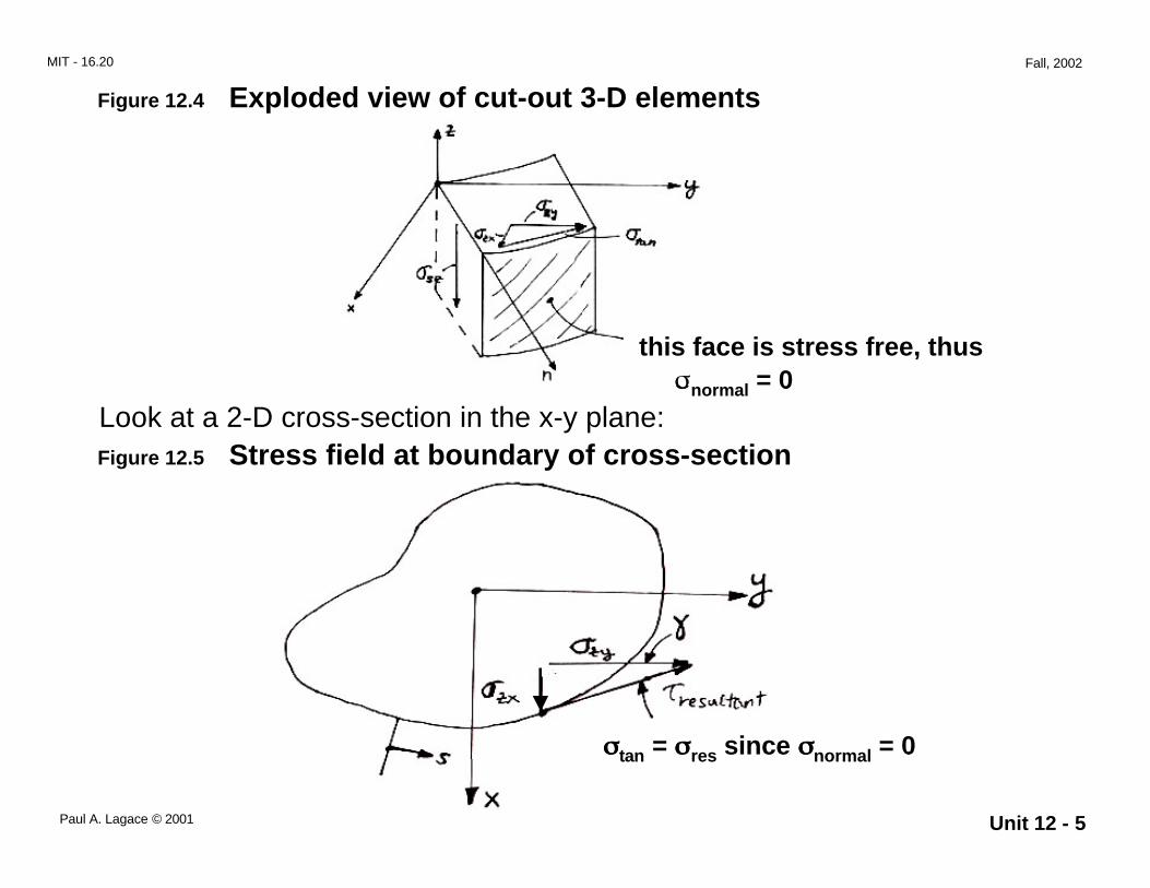
Figure 12.4 Exploded view of cut-out 3-D elements

this face is stress free, thus σnormal = 0

Look at a 2-D cross-section in the x-y plane: Figure 12.5 Stress field at boundary of cross-section

Paul A. Lagace © 2001

σσσσtan = σσσσres since σσσσnormal = 0

Unit 12 - 5

MIT - 16.20 Fall, 2002

τ resul tant = σzy cos γ + σzx sin γ

geometrically: cos γ =dy ds

dxsin γ =

ds

Thus: dx τ ds = ∫

dyds zy σ ds + σzx ds∫ ds

= ∫ σzy dy + σzx dx

We know that:

∂wσzy = G

kx +

∂y

σzx = G −ky + ∂w

∂x Paul A. Lagace © 2001 Unit 12 - 6

MIT - 16.20 Fall, 2002

⇒ = ∫ τ ds ∫ G kx + + ∫dy

∂w G −ky +

∂w dx ∂y ∂x

+ + ∫ dx Gdy k ∫∂w ∂w = G {xdy − ydx}

∂x ∂y

= dw

We further know that:

∫ dw = w = 0 around closed contour

So we’re left with:

∫ τds = Gk ∫ {xdy − ydx}

Paul A. Lagace © 2001 Unit 12 - 7

MIT - 16.20 Fall, 2002

Use Stoke’s Theorem for the right-hand side integral:

∫ ∂N ∂M{Mdx + Ndy} = ∫∫ ∂x

−∂y

dxdy

In this case we have

∂MM = − y ⇒ = − 1

∂y

∂NN = x ⇒ = 1

∂x

We thus get:

Gk ∫ {xdy − ydx} = Gk ∫∫ [1 − − 1)] dxdy(

= Gk ∫∫ 2dxdy

Paul A. Lagace © 2001 Unit 12 - 8

MIT - 16.20 Fall, 2002

We furthermore know that the double integral of dxdy is the planar area:

∫∫ ddxdy = Area = A

Putting all this together brings us back to Equation (12 - 1):

∫ = τds AGk 2Q.E.D.

Hence, in the general case we use equation (12 - 1) to relate C1 and C2. This is rather complicated and we will not do the general case here. For further information

(See Timoshenko, Sec. 115)

We can however consider and do the… Paul A. Lagace © 2001 Unit 12 - 9

τττ

MIT - 16.20 Fall, 2002

Special Case of a Circular Tube

Consider the case of a circular tube with inner diameter Ri and outer diameter Ro

Figure 12.6 Representation of cross-section of circular tube

For a solid section, the stress distribution is thus:

Figure 12.7 Representation of stress “flow” in circular tube

τres is directed along circles

Paul A. Lagace © 2001 Unit 12 - 10

MIT - 16.20 Fall, 2002

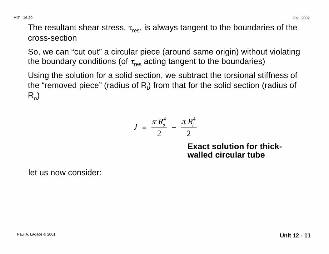
The resultant shear stress, τres, is always tangent to the boundaries of the cross-section

So, we can “cut out” a circular piece (around same origin) without violating the boundary conditions (of τres acting tangent to the boundaries)

Using the solution for a solid section, we subtract the torsional stiffness of the “removed piece” (radius of Ri) from that for the solid section (radius of Ro)

π R4 π R4

J = o − i

2 2

Exact solution for thick-walled circular tube

let us now consider:

Paul A. Lagace © 2001 Unit 12 - 11

MIT - 16.20 Fall, 2002

Thin-Walled Closed Sections

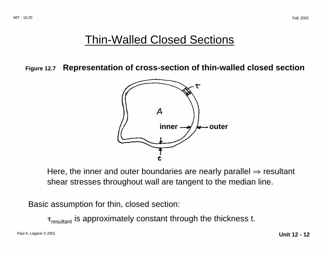
Figure 12.7 Representation of cross-section of thin-walled closed section

outer inner

Here, the inner and outer boundaries are nearly parallel ⇒ resultant shear stresses throughout wall are tangent to the median line.

Basic assumption for thin, closed section:

τresultant is approximately constant through the thickness t.

Paul A. Lagace © 2001 Unit 12 - 12

MIT - 16.20 Fall, 2002

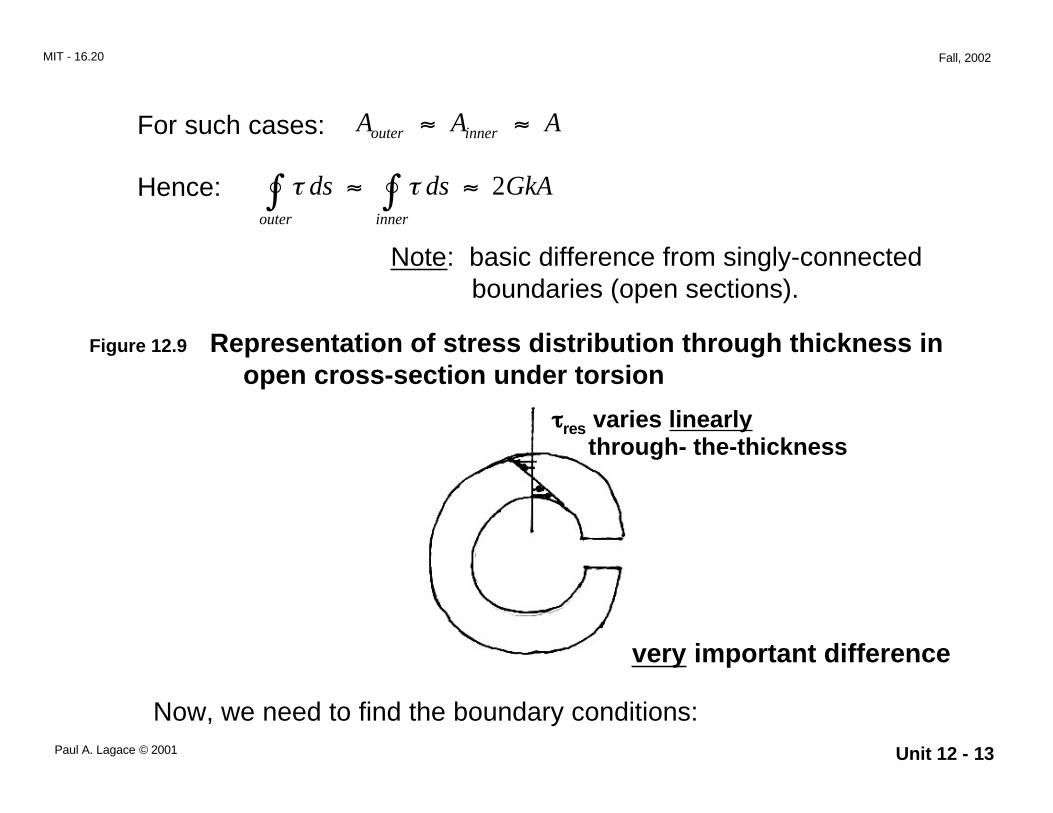
For such cases: Aouter ≈ Ainner ≈ A

Hence: ∫ τ ds ≈ ∫ τ ds ≈ 2GkA outer inner

Note: basic difference from singly-connected boundaries (open sections).

Figure 12.9 Representation of stress distribution through thickness in open cross-section under torsion

very important difference

ττττres varies linearly through- the-thickness

Now, we need to find the boundary conditions: Paul A. Lagace © 2001 Unit 12 - 13

MIT - 16.20 Fall, 2002

Figure 12.10 Representation of forces on thin closed cross-section under torsion

Force: dF = ττττ t ds

contribution to torque:

d T = hτ t ds

(h = moment arm)

Note: h, τ, t vary with s (around section)

Total torque = ∫ d T = ∫ τ t hds

Paul A. Lagace © 2001 Unit 12 - 14

MIT - 16.20 Fall, 2002

But τ t is constant around the section. This can be seen by cutting out a piece of the wall AB.

Figure 12.11 Representation of infinitesimal piece of wall of thin closed section under torsion

z

x-y plane

Use ∑ Fz = 0 to give:

−τ t dz + τ B tB dz = 0A A

⇒ τ tA A = τ B tB

in general: τ t = constant

Paul A. Lagace © 2001 Unit 12 - 15

MIT - 16.20 Fall, 2002

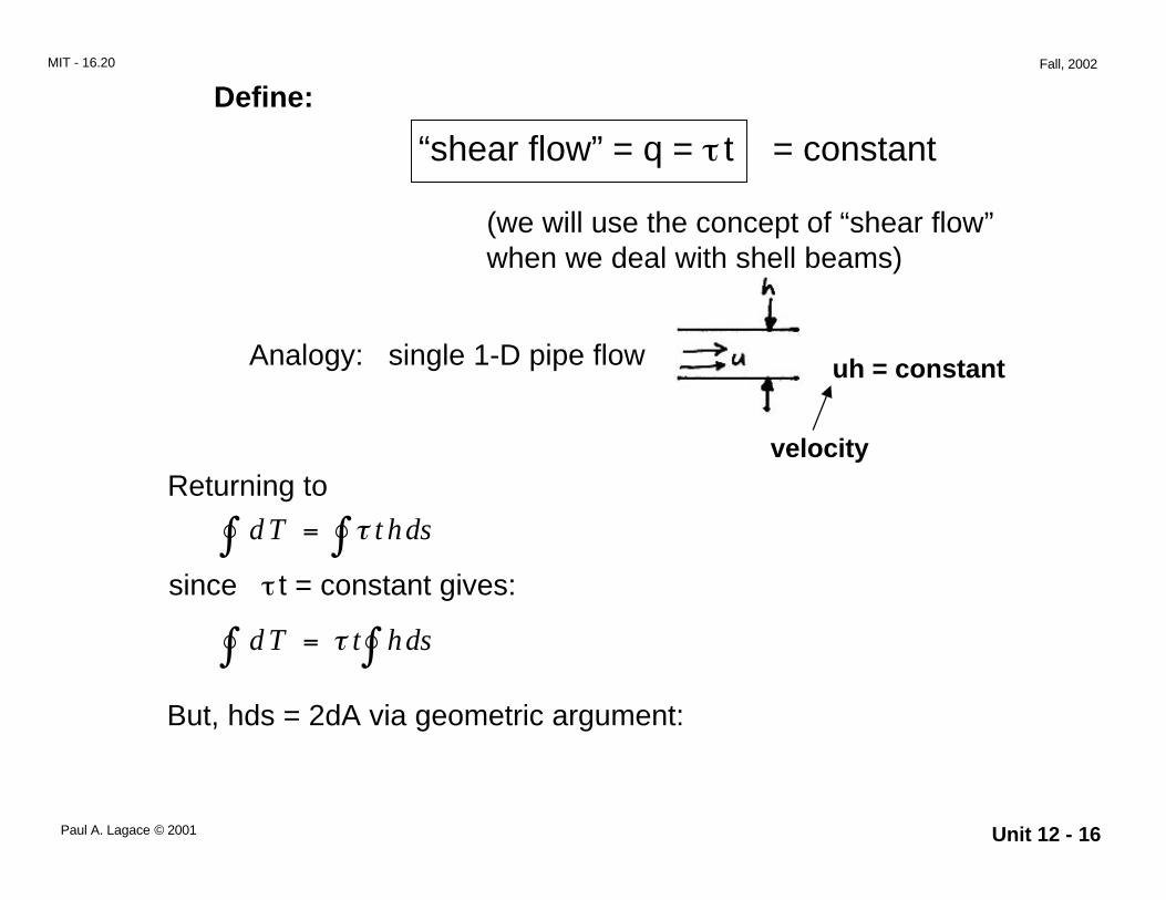
Define:

“shear flow” = q = τ t = constant

(we will use the concept of “shear flow”

Analogy: single 1-D pipe flow

when we deal with shell beams)

uh = constant

velocity Returning to

∫ d T = ∫ τ t hds

since τ t = constant gives:

∫ d T = τ t ∫ h ds

But, hds = 2dA via geometric argument:

Paul A. Lagace © 2001 Unit 12 - 16

MIT - 16.20 Fall, 2002

hdsdA =

2

height2x base

= Area TofTriangle

Finally:

⇒ d T t ∫ = τ ∫ 2 dA

⇒ T = 2τ t A T

⇒ τ resultant = 2At Bredt’s

(12 - 2)

formula Paul A. Lagace © 2001 Unit 12 - 17

MIT - 16.20 Fall, 2002

Now to find the angle of twist, place (12 - 2) into (12 - 1): T

ds = G k 2A 2At∫

T ds ⇒ k = ∫2 4A G t

This can be rewritten in the standard form:

dα Tk = =

dz GJ

4A2

⇒ J =

t

ds ∫

(Note: use midline for calculation)

valid for any shape…..

Paul A. Lagace © 2001 Unit 12 - 18

MIT - 16.20 Fall, 2002

Figure 12.12 Representation of general thin closed cross-section

How good is this approximation?

It will depend on the ratio of the thickness to the overall dimensions of the cross-section (a radius to the center of torsion)

Can explore this by considering the case of a circular case since we have an exact solution:

π R4 − π R4

J = o i

2

versus approximation: 4A2

J ≈ (will explore in home assignment)

t

ds ∫

Paul A. Lagace © 2001 Unit 12 - 19

MIT - 16.20 Fall, 2002

Final note on St. Venant Torsion:

When we look at the end constraint (e.g., rod attached at boundary):

Figure 12.13 Overall view of rod under torsion

Here, St. Venant theory is good

in this local region, violation of assumption of St. Venant theory

Built-in end

At the base, w = 0. This is a violation of the “free to warp” assumption. Thus, σzz will be present.

⇒ resort to complex variables (See Timoshenko & Rivello)

Paul A. Lagace © 2001 Unit 12 - 20