backdrop of this study is the

proposal by Basel Committee

on Banking Supervision to

adopt ES as a market risk

measure as an alternative to

the existing VaR measure.

Continuing on regulatory re-

quirements, the Dutch Cen-

tral Bank (DNB) introduced

the Internal Liquidity Ade-

quacy Assessment Process

(ILAAP) in the Netherlands

beginning June 2011, which is

in addition to the liquidity risk

management tools within

Basel III / CRD IV. Elmo Oli-

eslagers, Bert-Jan Nauta and

Aron Kalsbeek from Double

Effect, present a working pa-

per on Risk/ALM that recom-

mends the Dutch ILAAP as a

liquidity risk management tool

for Europe and a potential

tool to mitigate gaps in the

treatment of liquidity risk

within Basel III Pillar II re-

quirements.

The last article is by Jeroen

Hofman (Front Office Quant,

ING bank), who motivates the

development of a Graphical

Processing Unit (GPU) appli-

cation for estimation of liabili-

ties in a particular class of

variable annuity products,

namely the Single Premium

Variable Annuities (SPVAs).

We hope you will enjoy read-

ing this newsletter and we

look forward to seeing you at

the upcoming TopQuants

event(s).

Aneesh Venkatraman

(on behalf of TopQuants)

Dear Reader,

The TopQuants team is

pleased to present the first

issue of our 2014 newsletter

series. We are happy with the

positive feedbacks received on

our March and September

2013 newsletter issues and the

increased number of contribu-

tions. We encourage you all to

contact us with your ideas and

submissions which can include

technical articles, blogs, sur-

veys, book/article reviews,

opinions (e.g. on newly pro-

posed regulations), coverage

of interesting events, research

results from Masters/PhD

work, job internships etc.

This issue starts with a presen-

tation by De Nederlandsche

Bank (DNB), our host for the

upcoming TopQuants Spring

event in May 2014. Jon Vogel-

zang (Supervisor, Risk/ALM)

and Jantine Koebrugge (Policy

Advisor, Financial Risk Manage-

ment) share their experiences

as being part of the team within

DNB that is involved in the

preparatory work for the Euro-

pean Single Supervisory Mecha-

nism.

Some speakers (Joris van Vel-

sen, Roald Waaijer, Dimphy

Hermans, David Schrager, Tony

de Graaf, Robert Daniels, Cor-

nelis Oosterlee) from the No-

vember 2013 TopQuants Au-

tumn Workshop had enthusias-

tically responded by providing

summaries of their talks and

follow up research work which

have been included in this issue.

The summaries are very much

appreciated as they provide a

good recap of the talks and

also serve as a brief tutorial

on that topic.

This issue also features five

full length articles contrib-

uted by people from acade-

mia and industry. The first

article is by Eric Beutner,

Antoon Pelsser and Janina

Schweizer from the Maas-

tricht University who update

us on their research work in

the area of Least Square

Monte Carlo (LSMC) method

used for pricing complex path

dependent options. This is

an advancement of their

work presented in the first

issue of TopQuants newslet-

ter in March 2013.

The next two articles are

from Deloitte Financial Con-

sultancy Firm. Florian Reuter

and Arjan de Ridder highlight

the results and findings from

the recently conducted

Global Model Practice Survey

(GMPS) 2013, a biannual

initiative from Deloitte that

surveys global model prac-

tices within financial institu-

tions. This study emphasizes

on the increased use of com-

plex models within banks, the

associated model risks in-

volved and the need for ef-

fective Model Validation

teams within banks to man-

age model risk. In another

article, Gerdie Knijp and

Niek Crezée compare the

metrics of Value-at-Risk

(VaR) and Expected Shortfall

(ES) with regard to their ro-

bustness to different model

choices or assumption

changes in the model. The

Editorial

March 2014 Volume 2, Issue 1

TopQuants Newsletter

Inside this issue:

Editorial 1

Complex Financial

Products: The Icing on

the Cake

2

Lévy copulas: Basic

ideas and a new estima-

tion method

4

Replication of a Class

of Variable Annuities

for the Purpose of Eco-

nomic Capital Calcula-

tions

5

Variable Annuities —

Observations on valua-

tions and risk manage-

ment

6

Pension Fund — Asset

Risk Management

7

Stress Testing: A theo-

retical exercise or does

it actually work ?

8

Stochastic Grid Bun-

dling Method: A Tuto-

rial

9

Achieving super-fast

convergence in Least

Squares Monte-Carlo

11

Global Model Practice

Survey 2014: Validation

at Risk

13

Robustness of Expected

Shortfall and Value-at-

Risk in a Filtered

Historical Simulation

15

Liquidity Risk Manage-

ment in Europe: Base-

line Basel III Pillar II by

Dutch ILAAP

18

SPVAs: A Grid GPU

Implementation

24

The national competent authorities

(NCAs) of several countries participate

in this project amongst which is also

the De Nederlandsche Bank (DNB).

Jon Vogelzang is an econometrician and

currently works as financial risk man-

ager for DNB. Prior to that, he worked

for the PGGM pension fund company

and with ABN AMRO bank. Jon is

closely involved in the asset quality

review that DNB performs at the

seven ‘significant’ banks in the Nether-

Jon Vogelzang (Supervisor, Risk

and Asset Liability Management,

DNB) and Jantine Koebrugge

(Policy Advisor, Financial Risk

Management, DNB) are a part of

the team within DNB that is in-

volved in the preparatory work

for the European Single Supervi-

sory Mechanism. Together, they

provide a brief overview of the

work involved and share their

personal experiences as being

a part of this project.

check the valuation of more com-

plex and illiquid products (e.g. level

3 bonds, securitisations etc) and the

pricing models of derivatives. We

do this based on the guidelines set

by the European Central Bank

(ECB). It is an impressive 300-page

document with templates that pre-

scribe, which products have to be

considered and on which basis we

have to assess them.”

Over the past three months, the

Page 2 TopQuants Newsletter

Complex Financial Products: The Icing on the Cake - written by Jon Vogelzang and Jantine Koebrugge (DNB)

The European Banking Union will be-

come effective from November 4th

2014 onwards. To begin with a clean

slate, the balance sheets of all large

banks in the euro zone countries will

be assessed as part of the so-called

Comprehensive Assessment Project.

team of Jon was mostly focussed on

selection of those products and the

pricing models that exhibit the most

valuation risk.

Jon: “We agreed with the ECB on

the selection of products and port-

folios. Next, we can focus on the

lands. This is the part of the compre-

hensive assessment project which is

aimed at assessment of the balance

sheet and capital position of banks.

Jon: “The role of my team in this

project is to assess the fair value port-

folios of the banks. It is our task to

Jantine: ”The stress tests are devel-

oped in close cooperation with the

European Banking Authority (EBA).

This requires a lot of knowledge on

banking regulations and the models

that banks use for the stress tests.”

The scenarios for stress testing are

developed based on the economical

expectations of the European Com-

mission.

Jantine: “An example of a stress sce-

nario would be, increasing unemploy-

ment rates. Banks would use this sce-

nario to calculate the future impact

on their positions, for instance, where

will they possibly be in three years

from now. These scenarios are the

same for each bank in Europe, al-

though the implementation of the

stress test is done individually by the

banks. Every bank develops its own

models for this purpose and uses

their own data.”

Jon: “The Asset Quality Review en-

sures that all banks have valued their

asset in a similar manner, resulting in

the same starting point for each

‘significant’ bank in Europe. In this

way, we avoid comparing apples with

oranges.”

Jantine: “The ECB quality assurance

team benchmarks the results across

countries to ensure quality and con-

sistency of the analysis as much as

possible.”

Jantine: “What I like about this pro-

ject is that, the targets are clearly set

and we know the ‘head’ and ‘tail’ of

it. Further, we encounter many

challenges that we address together

as a team. Working with different

people is another reason why I en-

joy being a part of this project.”

assets and begin the investigation

process. For us, the complex financial

products are the icing on the cake.

These are mostly illiquid products for

which no market values are observed.

Using different models, we try to esti-

mate the market value of these prod-

ucts which is quite challenging. What

makes it more interesting is that,

every product is different and hence

we will have to employ new models

all the time in order to get as close as

possible to its “true” value.”

The ECB had decided that securitisa-

tions, mostly being repackaged mort-

gages, will have to be valued by a third

party. A good valuation team requires

people who are capable of under-

standing the complexities involved in

those products.

Jon: “Our team consists of seven

quants, all from different departments

in DNB. We work closely together

and discuss the possible approaches

which makes this project a great fun.

By the end of June, we hope to have

finalised the Asset Quality Review

(AQR), which will be used as input for

the stress tests.”

Stress testing

The stress test forms the final phase in

the comprehensive assesment project.

Jantine Koebrugge has been involved

from the start in this project. She had

joined DNB three years ago, her first

job in the industry after having ob-

tained her masters in financial mathe-

matics from University of Groningen.

Page 3 Volume 2, Issue 1

Disclaimer

Any articles contained in this newsletter express the views and opinions of their authors as indicated, and not

necessarily that of TopQuants. Likewise, in the summary of talks presented at TopQuants workshop, we strive to

provide a faithful reflection of the speaker's opinion, but again the views expressed are those of the author of the

particular article but not necessarily that of TopQuants. While every effort has been made to ensure correctness of

the information provided within the newsletter, errors may occur in which case, it is purely unintentional and we

apologize in advance. The newsletter is solely intended towards sharing of knowledge with the quantitative

community in the Netherlands and TopQuants excludes all liability which relates to direct or indirect usage of the

contents in this newsletter.

identify loss categories based

on business line and event

type. Next, the loss in each

category is modelled by a

compound Poisson process.

Finally, the annual losses of

different categories are con-

nected by a distributional

copula. The speaker then

explained the advantages of a

Lévy copula over a distribu-

tional copula in the context

of operational risk modelling.

Firstly, with a Lévy copula,

the nature of the model is

invariant with respect to the

level of granularity (i.e. if two

loss categories are merged,

the loss process of the new

category is again a com-

pound Poisson process).

Secondly, a Lévy copula al-

lows for a natural interpreta-

tion of dependence between

loss categories in terms of

common shocks.

Estimation and selection of a

Lévy copula between two

loss categories has been

studied in the literature in

case of known common

shocks (this corresponds to

continuous observation). In

practice, however, this infor-

mation is typically not avail-

able in operational loss data-

bases. The speaker high-

lighted his research work

which had resulted in devel-

oping a method to estimate

and select a Lévy copula of a

discretely observed bivariate

compound Poisson process.

Simulation results indicated

that the method works well

for sample sizes typically

encountered in operational

Distributional copulas play

an important role in finan-

cial modelling, although the

concept of a Lévy copula is

comparatively less well

known. In essence, a Lévy

copula provides the rela-

tionship between the Lévy

measure of a multivariate

Lévy process and the Lévy

measures of the associated

marginal processes. The key

application of a Lévy copula

is to parsimoniously specify

a multivariate Lévy jump

process via a bottom-up

approach.Against this back-

ground, the speaker focus-

sed on presenting the the-

ory of Lévy copulas and

their financial applications.

The presentation consisted

of two parts. Firstly, the

speaker, Joris van Vel-

sen,gave a general introduc-

tion of Lévy copulas and

discussed some important

applicationsfrom literature,

such as multi-asset option

pricing.Secondly, the

speaker presented a new

method to select and esti-

mate a Lévy copula for a

discretely observed com-

pound Poisson process. The

speaker emphasized the

usefulness of this method in

the area of operational risk

modelling.

To motivate his research,

the speaker began by dis-

cussing the industry prac-

tice of operational risk mod-

elling, which is typically

done by adopting a three-

step approach. Firstly, banks

risk modelling. Further, the

method has successfully been

applied to actual loss data.

Technical details about the

method can be found in the

pre-print http://arxiv.org/

pdf/1212.0092.pdf.

The presentation was well

received and resulted in lively

discussions about possible

extensions of the method and

future research. A presenta-

tion on the same subject had

previously been given by the

speaker at the 2012 Analytics

Forum of the Operational

Risk data exchange (ORX)

association, a world-wide

consortium of banks dedi-

cated to advancing the meas-

urement and management of

operational risk. The speaker

performed the research to

conclude a part-time study

Risk Management at the Dui-

senberg school of finance

(DSF) from 2010 to 2012.

For his performance during

the programme, the speaker

received the Best Students

Award for Risk Management.

— summarized by

Joris van Velsen

Lévy copulas: Basic ideas and a new estimation method - based on talk by Joris van Velsen (ABN AMRO)

“A new method to

select and estimate a

Lévy copula for a

discretely observed

compound Poisson

process is presented.

The methodology

enables the Lévy copula

to become a realistic

tool of the advanced

measurement approach

for operational risk.”

— Joris van Velsen

Page 4 TopQuants Newsletter

Replication of a Class of Variable Annuities for

the Purpose of Economic Capital Calculations - based on talk by Roald Waaijer and Dimphy Hermans (Deloitte)

“Allowing path

dependent instruments

in the replicating

portfolio results in a

more intuitive

instrument selection

and replicating

portfolios that better

capture the

sensitivities of variable

annuities”

—- Roald Waaijer and

Dimphy Hermans

Page 5 Volume 2, Issue 1

In recent years, life insurance

companies increas ingly

started using replicating port-

folio techniques for calculat-

ing economic capital. Key

difficulties occur in the repli-

cation of complex insurance

p roduct s w i th p a th -

dependent guarantees, such

as variable annuity products.

The speakers, Roald Waaijer

and Dimphy Hermans from

Deloitte FRM, the depart-

ment of Deloitte that focuses

on financial risk management

solutions for financial institu-

tions, discussed the replica-

tion of complex insurance

products by means of vanilla

instruments using a data min-

ing technique and compared

it with replication using ex-

otic options. This presenta-

tion included a general dis-

cussion on the use of repli-

cating portfolios for eco-

nomic capital calculations and

the difficulties in replicating

variable annuity products, the

visualisation of a data mining

technique and a case study

comparing the results of two

different replication ap-

proaches.

Deloitte has observed that

insurance companies employ-

ing replicating portfolio tech-

niques do manage to repli-

cate the path-independent

cash flow portion of their

portfolio. However, several

difficulties are experienced

when replicating products

with path-dependent cash

flows, for instance in the case

with variable annuities. Sol-

vency II and EIOPA have em-

phasized the difficulty in

replicating these products as

well. Variable annuities are

insurance products that

provide a series of payments

to the policyholder during

the entire fixed term of the

policy or, until the death of

the policyholder in case of a

life annuity. The level of

these payments depends on

the performance of the un-

derlying investment account.

For illustration purposes,

the speakers presented rep-

lication of a specific variable

annuity product, performed

using two different ap-

proaches. In the first ap-

p roach , on ly (pa th -

independent) vanilla instru-

ments were used for the

replication. Using cash flow

analysis, a likely candidate

asset set consisting of plain

vanilla instruments was se-

lected. Due to the mismatch

b e t w e e n t h e p a t h -

independent instruments

and the path-dependent

product, a data mining ap-

proach was required. How-

ever, the difference in risk

profile between the variable

annuity and the path-

independent instruments

still resulted in an imperfect

replication of the cash flows.

The second approach al-

lowed the insurer to use

both vanilla instruments and

path-dependent options for

replication, which resulted

in a more intuitive replicat-

ing portfolio.

The speakers then showed

the outcomes of a case study

in which the two different

approaches were compared. It

was shown that in case the

variable annuity was further

simplified, a perfect replication

could be found using the sec-

ond approach while in case of

no further simplification, no

perfect replication was found.

However, the use of path-

dependent instruments still

resulted in a better in-sample

replication quality and a better

sensitivity match between the

replicating portfolio and the

variable annuity when com-

pared with using only plain

vanilla instruments.

The talk was very well re-

ceived by the audience and led

to a lively discussion, which

included the computational

cost involved in using path-

dependent options for replica-

tion. The overall conclusion

was that, while a closed-form

valuation formula is not avail-

able for every path-dependent

instrument, the approach al-

lowing path-dependent instru-

ments in the replicating port-

folio results in a more intuitive

instrument selection and repli-

cating portfolios that better

capture the sensitivities of

variable annuities.

— summarized by

Roald Waaijer and

Dimphy Hermans

The speaker emphasised on

these two points in a very

lively and interesting manner.

According to him, we can

focus as much as we want on

more and more sophisti-

cated models, but if we can-

not get the simple vanilla

products right, we are al-

ready mispricing things to

such a large extent that the

typical profit margin on such

products quickly evaporates.

An important point to be

kept in mind is that the for-

ward price of assets has to

include the repo rate, as has

been pointed out in many

technical papers that were

written since the crisis, for

instance refer to e.g. Piter-

barg. The widening cross-

currency basis is another

factor to take into account.

Secondly, behavioural or

lapse risk is pivotal to the

valuation of VAs and it

should also be taken into

account in such products. It

is wrong to assume that cli-

ents will walk away from

their variable annuity con-

tracts in a rational manner.

The speaker highlighted his

research work done to-

gether with the co-authors

in which they have at-

tempted to model this lapse

behaviour in a simple manner

based on how much the cur-

rent market levels differ

from the guarantee embed-

ded within the contract.

Based on this functional

form, one can attempt to

structure financial derivatives

(“building blocks”) from

which the value of the vari-

Variable Annuities (VA) have

increasingly become a widely

used instrument in retire-

ment planning, especially in

countries like America and

Japan where it amounts to

billions of euros of premiums

every year. Further, there is

expected to be increasing

demand for VA in the future

as more people, particularly

from developed countries live

longer healthier lives. In

short, VA are the answer to

the demand for private (3rd

pillar) pension products.

Against this background, the

speaker David Schrager, Sin-

gle Premium Variable Annuity

Trading at ING Bank, had

contributed with a presenta-

tion on variable annuities

which included a general in-

troduction to VA, note on

industry practices for their

valuation and hedging and

how to efficiently deal with

policyholder behaviour in the

valuation of these products.

There were few other talks

on VA during the TopQuants

workshop. In particular, the

talk by Roald Waaijer and

Dimphy Hermans focussed

more on how to replicate a

VA using existing instruments

in order to speed up eco-

nomic capital calculations

while David Schrager had

focussed on two important

aspects of the pricing of VAs;

basis risk arising due to

wrong choice of discount

curve and behavioural or

lapse risk arising due to the

client's early surrender.

able annuity can be built. If

values of these building

blocks can be obtained in

the market, it will facilitate

the pricing of VAs. The esti-

mation of the degree of irra-

tionality however remains,

and is an important risk in

these products.

The speaker concluded the

talk by presenting an illustra-

tive case study that involved

hedging of VAs. Overall, the

talk was well received by

the audience and had led to

a lively after discussion.

— summarized by

Roger Lord and

Aneesh Venkatraman

Variable Annuities — Observations on

valuations and risk management - based on talk by David Schrager (ING)

“We can focus as much

as we want on more

and more sophisticated

models, but if we

cannot get the simple

vanilla products right,

we are already

mispricing things to

such a large extent that

the typical profit

margin on such

products quickly

evaporates”

— David Schrager

Page 6 TopQuants Newsletter

idea of how volatile their cov-

erage ratio is: the Coverage

Ratio at Risk (CRaR). This

statistic presents the worst

coverage ratio that the board

can expect within a given cer-

tain horizon and confidence

level. The CRaR can be attrib-

uted to different asset classes

and/or different investment

decisions. Typically an ALM

study comes first followed by

the Strategic Benchmark and

finally the implementation. For

each of these decisions and

each step in the investment

process, the effect on the

CRaR can be determined.

Liquidity and controllability

During the 2008 crisis, some

pension funds were con-

fronted with liquidity con-

straints, especially when they

had implemented large deriva-

tive overlay structures. The

speaker presented a risk

dashboard which shows for a

certain stress scenario, the

required or available liquidity

for each asset class and over-

lay, including the effects of

possible repo market actions

and rebalancing schemes.

Controllability then measures

to what extent the resulting

asset mix can be steered back

to the strategic mix.

Risk attribution

Risk attribution is a useful tool

for risk managers that can be

applied in very different set-

tings. The speaker highlighted

its use in balance sheet risk

management and presented

the mechanics of risk attribu-

tion for widely used risk sta-

Currently, there is an in-

creasing need for pension

fund boards to be ‘in con-

trol’, perhaps much more

than it previously used to

be. They demand, among

many things, transparency,

robust processes and good

governance from their dele-

gated investment managers.

They prescribe detailed

compliance rules and expect

to receive comprehensive

reporting on their invest-

ment portfolios, certainly on

the risk side. The speaker,

Tony de Graaf, had dis-

cussed several popular in-

vestment risk reporting

items and offered some new

ideas, focusing mainly on the

public markets investment

portfolios. A short summary

of these risk reporting ele-

ments is provided, which

should be considered as a

toolbox, but certainly not an

exhaustive set.

Balance sheet risk measure-

ment

Investment managers some-

times have a tendency to

narrow their focus on cer-

tain portfolios, especially

when they manage only part

of the pension assets. How-

ever, pension fund boards

always look first to obtain a

risk report that gives them

immediate insight into the

main risks of their fund.

Coverage ratio is a very

important financial statistic

employed by pension funds

in the Netherlands. In this

regard, the speaker has de-

veloped a dashboard that

gives pension board a good

tistics like Value-at-Risk,

Tracking Error, Expected

Shortfall, in a way that is simi-

lar to the more commonly

used technique of perform-

ance attribution. Risk and

performance attribution

measures complement each

other and together they quan-

tify all investment decisions

made by a portfolio manager,

from both a risk and a return

perspective. The total risk

and performance can be at-

tributed to allocation and

selections decisions, to risk

types, country/region, style,

strategy, instrument type etc.

These attributions can be

calculated either separately or

can also be nested, e.g. first

per forming a l loca t ion /

selection and then attribution

to the different regions where

the portfolio manager invests.

The speaker presented this

for both the classical ap-

proach and a new approach

formulated by himself. This

new method provides more

flexibility and intuitive out-

comes, although being more

computationally intensive.

Other topics discussed in-

clude stress testing, style

analysis, AIFMD. The speaker

engaged with the audience on

topics like technologies used

in these Risk Management

toolkits, calculation run time,

applicability of the tools for

non-linear products, system-

atic risk coverage within the

risk management tool etc.

— summarized by

Tony de Graaf

Pension Fund — Asset Risk Management - based on talk by Tony de Graaf (PGGM)

“Financial risk

measurements within

asset management

only become fully

useful when combined

with methods able to

zoom in, top down,

and show the risk

contributions made by

the various

components and

decisions made in the

investment

management process”

— Tony de Graaf

Page 7 Volume 2, Issue 1

Page 8 TopQuants Newsletter

Stress Testing: A theoretical exercise or does it actually work ? — by Robert Daniels (Partner at Capstone Financial Industry)

Why are we surprised when the outcome of a stress scenario

is far worse than what was predicted? Often we tend to ra-

tionalize the outcome e.g. “it was a four sigma event” or “it

was a black swan”. However, could it be the case that the

applied stress test methodologies are inherently weak? If so,

how can a risk modeler/manager communicate these weak-

nesses to senior management or even on a board level? In

this article an overview is given of commonly applied stress

test methodologies including some practical challenges for risk

modelers and risk managers.

Stress tests are widely performed for many years

so what is new?

This is true. Many organizations are performing stress

tests as part of their standard risk management frame-

work. However during the recent crises the limitations

of these stress tests have been revealed e.g. for several

portfolios a Value-at-Risk of losses under stress tests

were estimated of less than a million, whilst actual losses

exceeded several billions. Therefore, one of the ques-

tions that is on the table is how a framework can be

setup that aims at identifying weaknesses under stressed

circumstances.

Combining macro-economic and risk models for

stress testing: The Holy Grail or a recipe for dis-

aster?

One of the most commonly applied stress test method-

ologies is to relate macro-economic variables to risk

parameters and based on these risk parameters the

stress impact is assessed. Even though this approach

seems logical it is an inherent weak approach. Both

macro-economic and risk models are weak to predict

the impact of stressed circumstances and lead to a situa-

tion as illustrated in this figure below.

But what is driving this disconnect? Macro-economic mod-

els are known for their weak predictiveness, even under

normal circumstances. In addition, there are factors that

play an important role during times of stress for example

hidden (contractual) optionalities, non-linearities in pay-off

structures and behavior of financial markets and market

participants. Surprisingly, these factors are often forgotten

by (quantitative) risk managers even though they drive the

outcome under stress significantly.

The “Risk management please provide one num-

ber for the outcome of a stress test” syndrome

If you often perform stress tests then you know what I am

talking about. Senior management often requires risk man-

agement to provide a clear, one figure impact of a stress

test. From my experience this approach gives a false sense

of security to senior management. Also a one figure impact

does not provide senior management the right tools to

timely mitigate the effects if an event occurs.

A different method would be to define multi-stage stress

tests in which an event occurs in various stages. The bene-

fit of this approach is that the impact for each stage can be

estimated in terms of the balance sheet, P&L, markets and

the business model itself. Besides focusing on the impact, it

leads also to discussion on what to do when an event ma-

terializes. For example, can triggers be defined in an early

stage such that a discussion takes place on the measures

to be taken at that time?

This approach does require a lot of knowledge of course.

Not only regarding risk models, but also from financial

markets and behavior of market participants. The key of

success is therefore in the creativity and knowledge of a

risk manager when defining stress tests. On the other

hand, blaming external factors such as “four-sigma events”

or “black swans” are still tempting as little knowledge and

no action is required.

Robert Daniels holds M.Sc. in financial

econometrics and M. Phil in economics.

He is partner at Capstone Financial

Industry and Daniels Risk Advisory. His

aim is to provide fundamentally sound

solutions to financial institutions in the

field of strategic risk management and

effective decision making.

Page 9 Volume 2, Issue 1

Abstract

This note describes a practical simulation-based algo-

rithm, which we call the Stochastic Grid Bundling Method

(SGBM) for pricing multi-dimensional Bermudan (i.e. dis-

cretely exercisable) options. The method generates a

direct estimator of the option price, an optimal early-

exercise policy as well as a lower bound value for the

option price. An advantage of SGBM is that the method

can be used directly to obtain the Greeks (i.e., derivatives

with respect to the underlying spot prices, such as delta,

gamma, etc) for Bermudan-style options. Computational

results for various multi-dimensional Bermudan options,

presented in [1], demonstrate the simplicity and efficiency

of the algorithm proposed.

Stochastic Grid Bundling Method

A Bermudan option gives the holder the right, but not

obligation, to exercise the option once, on a discretely

spaced set of exercise dates. Pricing of Bermudan options,

especially for multi-dimensional processes is a challenging

problem owing to its path-dependent settings.

Consider an economy in discrete time defined up to a

finite time horizon T . The market is defined by the fil-

tered probability space

Let,

be an -valued discrete time Markov process that

describes the state of the economy, the price of the un-

derlying assets and any other variables that affect the dy-

namics of the underlying. Here, Q is the risk neutral

probability measure. The holder of the Bermudan option

can exercise the option at any of the discrete times

(1.1)

Let represent the cash flow received when the

option is exercised at t , with underlying state being

We define a policy, π, as a set of stopping times τ which

can assume any of the discrete time values in equation

(1.1). The option value is found by solving an optimiza-

tion problem, i.e. to find the optimal exercise policy, π, for which the expected cash flow is maximized. This can

be written as:

(1.2)

In simple terms, equation (1.2) states that of all possible

exercise policies in the given decision horizon, the option

value is the one which maximizes the expected future

cash flows. SGBM solves a general optimal decision time

problem using a hybrid of dynamic programming and

Monte Carlo simulation. The steps involved in the SGBM

algorithm, can be summarized as follows:

Step I: Generating grid points

The grid points in SGBM are generated by simulating in-

dependent copies of sample paths,

of the underlying process and all starting from the

same initial state The grid point at time

is given by:

,

Depending upon the underlying process an appropriate

discretization scheme, e.g. the Euler scheme, is used to

generate sample paths. Sometimes the diffusion process

can be simulated directly, essentially because it appears in

a closed form, as an example, for the regular multi-

dimensional Black-Scholes model.

Stochastic Grid Bundling Method: A Tutorial

— by Cornelis Oosterlee (Delft University of Applied Mathematics)

dR

.tX

Page 10 TopQuants Newsletter

Step II: Option value at terminal time

The option value at terminal time is given by:

.

This relation is used to compute the option value for all

grid points at the final time step. The following steps are

subsequently performed for each time step, with

m ≤ M, recursively, moving backwards in time, starting

from

Step III: Bundling

The grid points at are bundled into

non-overlapping sets or partitions. Three different ap-

proaches for partitioning are considered, they are:

1. K - means clustering algorithm,

2. Recursive bifurcation,

3. Recursive bifurcation of reduced state space.

These techniques are detailed in [1].

Step IV: Mapping high-dimensional state space to

a low-dimensional space

Corresponding to each bundle

,

a parameterized value function,

which assigns values to states is

computed. Here, is a vector of free

parameters. The objective is then to choose, for each

and β, a parameter vector so that

The parameter vector is determined by means of regres-

sion.

Step V: Computing the continuation and option

values at

The continuation values for

are approximated by

The option value is then given by:

This procedure is repeated over all time steps, backward in

time, until the initial time point is reached.

References

[1] Shashi Jain and Cornelis Oosterlee, The Stochastic Grid

Bundling Method: Efficient Pricing of Bermudan Options

and their Greeks(September 4, 2013). Available at SSRN:

http://ssrn.com/abstract=2293942

Page 11 Volume 2, Issue 1

Introduction

The Least Squares Monte Carlo (LSMC) technique is

widely applied in the area of Finance, especially in pricing

high-dimensional Bermudan/American-style options, where

closed-form solutions are not available. Under LSMC the

cross-sectional information inherent in the simulated data

is exploited to obtain approximating functions to condi-

tional expectations through performing least squares re-

gressions on the simulated data. Simulation-based regres-

sion methods are also applied in insurance risk manage-

ment as a technique to estimate the value of (Life and

Health) insurance liabilities. Essentially these techniques are

used to estimate unknown conditional expectations across

time, which in Finance and insurance boils down to esti-

mating the price of a contingent claim, for which closed-

form solutions are not available. In this article we discuss a

particular LSMC estimator, for which convergence in mean

square faster than Ν⁻¹ can be achieved. This article is

based on the key results in Beutner et al. (2013).

The point in time of regression matters!

The majority of the academic literature deals with LSMC

estimators where the conditional expectation function

(pricing function) at time t is estimated through least

squares regression of the value function at a time point T

against basis functions at an earlier time point t, t < T. The approach is known as Regression-Now (Glasserman

and Yu, 2004). An alternative approach, termed Regression

-Later, approximates the value function at time T through

regression on basis functions measurable with respect to

the information available at time T. The estimate for the

price at time t is then obtained by pricing the basis func-

tions. Although similar, Regress-Now and Regress-Later

are fundamentally different.

Regress-Later can achieve a convergence in mean-

square that is faster than Ν⁻¹ which Regress-Now

cannot. The functions to be approximated with regression on

the Monte Carlo simulation set may differ in nature.

In this article we address the first point.

The technical set-up

We consider here a very simple set-up and omit techni-

cal details. This should allow the reader to quickly see

the difference between LSMC with Regress-Now and

with Regress-Later. We restrict attention to contingent

claims with finite second moments. This allows us to

model the contingent claims in a Hilbert space. From

Hilbert space theory we know that an element of a sepa-

rable Hilbert space is expressible in terms of an infinite,

but countable orthonormal basis. As we cannot estimate

infinitely many parameters based on finite samples for

estimation purposes the expression must be truncated.

Thus, we can express X through a finite linear combina-

tion of basis functions plus an approximation error,

which arises from truncating the basis. Now, recall that

in Regress-Now the basis functions refer to an earlier

time point t, t < T. By regressing X against basis func-

tions at time t the conditional expectation with respect

to information at time t is directly estimated. Then, addi-

tional to an approximation error a projection error is

realized arising from the time-difference. Let X be the

payoff at time T of a contingent claim. In a very simple

set-up let Z(T) be the underlying random variable driving

the random payoff X at time T. The basis functions are

denoted by еᵢ .

Regression equation with Regress-Later

Regression equation with Regress-Now

where err₁ and err₂ refer to approximation and pro-

jection error respectively. In estimating the above, the

truncation parameter K is not fixed and finite but grows

with the sample size. Thus, in the limit, the approxima-

tion error vanishes for both Regress-Now and Regress-

Later.

Achieving super-fast convergence in Least Squares Monte-Carlo

— by Eric Beutner, Antoon Pelsser, Janina Schweizer (Maastricht University)

Page 12 TopQuants Newsletter

Super-fast convergence

The convergence rates in mean-square for Regress-Now

and Regress-Later are functions of the sample size, N, and

the number of basis terms, K(N). The explicit conver-

gence rates below are taken from Beutner et al. (2013).

Convergence rate for Regress-Later:

Convergence rate for Regress-Now:

The potential super-fast convergence in Regress-Later is

achieved as the regression problem is non-standard.

From the previous explanations we can see that the ap-

proximation error decreases as the sample size grows.

This follows as the truncation parameter K is an increas-

ing function of the sample size. In Regress-Now also the

approximation error converges to zero as the sample size

grows, but the projection error remains. We can see that

the Regress-Now convergence rate has an additional

term, which arises from the projection error. If the target

function is in the span of finitely many basis functions the

approximation error in Regress-Now vanishes and only

the projection error is left. Then, the Regress-Now esti-

mator converges at rate Ν⁻¹, which is its maximum con-

vergence rate. The ultimate convergence rate of the Re-

gress-Later estimator is given by the convergence rate

stated above and the growth relation of the truncation

parameter and the sample size. Note that intuitively the

growth rate of K in relation to the sample size must be

restricted as for a given sample size only a limited number

of parameters can be estimated.

We illustrate the super-fast convergence with normalized

non-overlapping piecewise linear functions, which are by

construction orthonormal. In the first example we con-

sider a hyperbolic function. In the second example we

consider a stock modelled as a geometric Brownian mo-

tion. The underlying drivers are Brownian motions. In the

first example a convergence rate of Ν⁻² is achieved (see

top figure), in the second case the convergence rate is still

faster than Ν⁻¹ (see bottom figure).

Conclusion

In this short article we discussed two types of LSMC, Re-

gress-Now and Regress-Later, and illustrated that for Re-

gress-Later convergence faster than Ν⁻¹ can be achieved.

This renders Regress-Later a very interesting alternative to

the typically applied Regress-Now estimators in LSMC.

References

Beutner, E., Pelsser, A., and Schweizer, J. (2013). Fast con-

vergence of Regress-Later estimates in Least Squares

Monte Carlo. http://papers.ssrn.com/sol3/papers.cfm?

abstract_id=2328709. Working Paper. Glasserman, P. and Yu, B. (2004). Simulation for American

options: Regression now or regression later? In Monte

Carlo and Quasi-Monte Carlo Methods 2002, pages 213-226.

Springer Berlin Heidelberg.

Page 13 Volume 2, Issue 1

Introduction

Increasing model complexity has given rise to a new type of risk faced by financial institutions: model risk. Both regula-

tory regimes and financial institutions have taken steps to address this type of risk. The cornerstone in managing model

risk is an independent Model Validation function. Model Validation provides an objective review to Model Develop-

ment, hence addressing the issue of model risk. Furthermore, Model Validation plays an important role in assessing the

compliance of models to internal and external regulations. As a result, Model Validation provides comfort to the stake-

holders in the use of the models and thereby improves model-based decision making within an organization. Currently,

the practices of Model Validation activities vary among financial institutions.

Every two years, Deloitte conducts the Global Model Practice Survey (GMPS) a global survey on model practices

within financial institutions. The latest edition of the survey was conducted in the second half of 2013 and focused on

the state of the Model Validation function within financial institutions. The survey was conducted among 96 financial

institutions globally, of which 15 based in The Netherlands. The respondents represent different geographies, indus-

tries, sizes and structures. Based on the completed set of responses we provide insight into the operation of Model

Validation within various organizations. The key findings of the survey are listed below.

Model Validation has become an established practice

The added value of Model Validation for the business is being increasingly recognized, i.e. all survey respondents indi-

cated that Model Validation adds value and the majority of the respondents acknowledge the technical expertise of

Model Validation. Other functions, such as Risk Management and Model Development, also recognize the important

role of Model Validation as mitigant of model risk. On the other hand, the most frequently cited reason for having a

Model Validation function is still regulatory compliance. Figure 1 presents the added value of Model Validation for the

business, as perceived by Model Validation and other roles. Here, we see a misalignment in perception of Model Vali-

dation versus its stakeholders regarding the value added by Model Validation.

Figure 1: Perceived added value of Model Validation for the business

The survey results demonstrate that Model Validation processes are becoming more mature and standardized. Com-

pared to the GMPS 2011, significantly more respondents indicate that the ownership of the model inventory is formal-

ized. This development improves the oversight of the model landscape within the financial institutions and herewith

also the control framework.

Global Model Practice Survey 2014: Validation at Risk

— by Florian Reuter and Arjan de Ridder (Deloitte Financial Risk Management)

Page 14 TopQuants Newsletter

However, it is still not a mature activity

Despite the achievements made over the last two years, there is still significant room for improvement. Many respon-

dents indicate that Model Validation is still at its infant stage. Difficulties are experienced in adhering to the model vali-

dation cycle and the advice of Model Validation to reject or substantially remediate a model, is often not followed. In

addition, defining and documenting roles and responsibilities of Model Validation is considered to be challenging. In

particular, for institutions with a decentralized Model Validation function or financial institutions without an independ-

ent Model Validation function, these roles and responsibilities are often not adequately documented.

The survey results indicate that in many cases Model Validation only covers regulatory models and that these models

require more personnel to cover the desired scope. In addition, in order to be compliant with (future) regulations, a

substantial part of the respondents would like to broaden the scope of activities performed by Model Validation. For

example, by expanding the use of validation tools. Figure 1 shows an overview of validation tools currently used by the

respondents.

Figure 2: Average percentages of validation tools used by the aggregate financial industry

Respondents also indicate that they would like to increase the size of the team. Although respondents repeatedly state

that Model Validation is “an under-staffed function”, it is also frequently considered to be an “expensive function con-

strained by available resources”. Partially due to these (temporary) insufficient resources, about half of the respon-

dents outsource model validation work to external parties.

Finally, the current state of performance assessment of the Model Validation function does not indicate a sufficient

maturity of the function. In particular, a quarter of the respondents indicate to have no Key Performance Indicators

for Model Validation.

Model Validation within banks is more mature than within other industries

Model Validation appears to be more mature at banks than at other institutions. Almost all banks have a centralized

Model Validation function within the domain of Risk Management. Other industries often have a decentralized Model

Validation function where responsibilities are less clearly defined or do not have an independent Model Validation

function at all. Banks also assign on average more FTE resources to Model Validation although the average model vali-

dation working experience is lower for banks. Larger departments (more common for banks) seem to have relatively

fewer seniors and more juniors.

Going forward

We asked the respondents to provide their vision on the development of the Model Validation function in the next

three years. The general consensus is similar to the survey of 2011: the respondents believe the importance and

prominence of Model Validation to continue to increase in the future. Varying reasons for the increasing importance

Page 15 Volume 2, Issue 1

and prominence are provided. One is the continued increase in regula-

tory expectations for Model Validation. The regulation of financial institu-

tions is expected to become even more stringent. Banks today still face

challenges in implementing Basel II whereas Basel III is already imminent.

The European insurers have to comply with Solvency II directive while

upcoming and existing regulation for investment managers, pension funds

and other financial institutions is increasing both in aggregate and with

greater emphasis on quantitative requirements.

Finally, the survey results indicate that the main challenge faced by Model Validation is to move from a predominantly

compliance function into a business partner which proactively manages model risk and ultimately promotes better us-

age of models within an organization. The full report can be found here.

Introduction

One of the objectives of the Basel Committee is ensuring consistency of market risk-weighted asset (mRWA) out-

comes. Recently several regulators (BIS and IMF) have published papers (Basel Committee on Banking Supervision,

2013), (Avramova & Le Leslé, 2012), in which they show that the mRWAs calculated for similar portfolios differ across

countries and banks. These variations are not only due to different risk profiles or different supervisory rules but it is

presumed that a significant part of the variability in mRWAs is caused by different methodology choices of banks. This

negatively affects market confidence and therefore there is need for a revision in the regulatory framework.

At the same time, the Basel Committee on Banking Supervision (BCBS) presents a number of propositions for a revi-

sion of the trading book (Basel Committee on Banking Supervision, 2013), as it is recognised that the old framework

has some significant shortcomings. One of the considerations described in the second consultative document of the

Fundamental Review of the Trading Book, is a change of the market risk metric on which the mRWAs should be de-

termined in an internal model based approach. BCBS proposes the use of expected shortfall (ES) at a 97.5% confidence

interval as an alternative for the widely used value-at-risk (VaR), measured at a 99% confidence interval.

Whereas VaR simply measures the quantile of the loss distribution, ES measures the expected loss of a portfolio given

that the loss has exceeded a certain quantile. It therefore takes tail risk into account. Following the Basel propositions,

we compare a 99% VaR with a 97.5% ES. This comparison stems from the normal distribution, as the two are approxi-

mately equal if the underlying distribution is normal.

Considering the observed variability in mRWAs measured under VaR, we analyse the sensitivities of certain assump-

tions on the VaR and ES measures. Particularly now that ES is proposed as replacement for VaR, we consider it worth-

while to investigate how this transition would affect the consistency of mRWAs among firms with similar risk profiles.

We will analyse the robustness of VaR and ES, where we define robustness as the sensitivity of market risk measures

towards certain model choices or assumption changes in a model.

Filtered Historical Simulation

We use filtered historical simulation (FHS) to calculate VaR and ES. FHS is a widely acknowledged method in

(academic) literature. It is a semi-parametric technique which uses bootstrapping and combines historical simulation

with conditional volatility modelling. FHS takes volatility clustering into account which makes it a more advanced

“The value and importance of model

validation will further rise because of

new regulatory requirements”

Group Manager of Risk Model

Validation department of a bank

Robustness of Expected Shortfall and Value-at-Risk in a Filtered

Historical Simulation Framework — by Gerdie Knijp and Niek Crezée (Deloitte Financial Risk Management)

Page 16 TopQuants Newsletter

method than simple historical simulation. FHS generates scenarios of risk factor returns from which VaR and ES can be

calculated.

We include several conditional volatility models, namely a simple GARCH model, the asymmetric GJR-GARCH model

and an EWMA model, which is used in RiskMetrics, as these models have proven to work well in practice and are

commonly used within financial institutions. These models cover symmetric and asymmetric conditional volatility mod-

els and models with and without mean reversion.

Empirical analysis

We constructed a portfolio consisting of simple equity and fixed income products. Risk factors to which these prod-

ucts are exposed are equity indices, short- and long-term interest rates and short- and long-term credit spreads for

different credit ratings.

The main analysis of robustness of VaR and ES is done by investigating the sensitivity of these risk measures towards

parameter modifications. We perform small modifications towards the different parameters underlying the conditional

volatility models and investigate the effect on VaR and ES using the theory of influence functions (Hampel, et al., 2011).

Influence functions are widely used in robustness analysis and can easily be adapted towards our investigation purpose.

This influence curve is defined by:

where represents a certain estimated parameter in the conditional volatility model, is the empirical loss

function followed from the FHS process and T is a statistic which is in our case VaR or ES.

We calculate approximations of the influence functions with respect to different parameter changes for VaR and ES at

different points in time. This gives us a time series of sensitivity estimates for both VaR and ES for different parame-

ters. We make a distinction in sensitivity effects due to changes in parameters in short-term interest models, long-

term interest models and equity.

Figure 1 shows such a time series of the influence curve, based on a change in in the EWMA model for long term

interest. From the pattern observed, we see that the sensitivity of VaR can become much more extreme than sensitiv-

ity of ES. For other parameters, asset classes and models, similar patterns occur, from which we expect VaR being

more sensitive towards small parameter modifications than ES.

To confirm this hypothesis, we perform simple linear regressions on the difference of the absolute value of the sensi-

tivity parameter of VaR and ES over time. We analysed the effect of changes in different estimated parameters from

the conditional volatility models, namely The estimated parameters for the different conditional

volatility models are: (1) GARCH (1,1) (2) EWMA(1,1):

(3) GJR - GARCH(1,):

We formulated two hypotheses to test for differences in robustness properties of VaR and ES. We first test whether

the difference of the absolute values of the influence function of VaR and ES is equal to zero or not:

Page 17 Volume 2, Issue 1

This is done by regressing the difference of the absolute values of the influence functions of VaR and ES on a constant.

By performing a t-test on the estimated intercept we test whether the estimated difference in absolute values of the

influence functions of both measures is zero or not. We take into account that the residuals are possibly subject to

autocorrelation and heteroskedasticity and therefore we use Newey-West standard errors. We find that this hypothe-

sis can be rejected for all parameters, asset classes and models, meaning that there is enough evidence to state that the

difference between the absolute value of the influence functions of VaR and ES is significantly different from zero. From

the estimated coefficients, the patterns of the influence functions and the corresponding summary statistics, we can

conclude that VaR is more sensitive towards parameter modifications than ES in a FHS framework.

Second, we test for dependence of this difference on conditional volatility, by defining a second hypothesis:

with either the intercept c ≠ 0, the coefficient β ≠ 0, or both. The parameter represents the conditional volatility

at time t. This hypothesis is tested by performing a linear regression where we also regress on the corresponding con-

ditional volatility. By performing both t-tests and an F-test on the estimated coefficients we test whether there is evi-

dence for the difference of the absolute values of VaR and ES being dependent on conditional volatility. From the

regression results regarding we again find that VaR is more sensitive towards small parameter modifications than

ES. Moreover, there is some evidence for the difference in absolute value of the influence functions of the two

Figure 1: Time series of the influence curve of VaR en ES based on modifications in in the

EWMA model for long term interest

Page 18 TopQuants Newsletter

measures being dependent on conditional volatility. However, this effect is not unambiguous for the different parame-

ters, models and asset classes.

Concluding remarks

The result that VaR is less robust than ES is not in line with earlier studies. In literature it is proven that historical ES is

unbounded in terms of the addition of extreme observations and thus more sensitive to extreme outliers than VaR

(Cont, et al., 2010). However, VaR and ES are often compared at the same confidence level. Also, robustness is often

investigated by means of sensitivity analysis where extreme observations are added to a dataset, rather than by means

of modifications in model assumptions. We executed a different, more realistic, approach to test for robustness, since

we constructed a portfolio for which VaR and ES are calculated using historical data of risk factors.

Our analysis showed that ES is less sensitive towards certain model choices, indicating mRWAs are less likely to vary a

lot among banks with similar profiles when ES is used as a market risk metric.

Bibliography

Avramova, V. & Le Leslé, S., 2012. Revisiting risk-weighted assets. International monetary fund (IMF).

Basel Committee on Banking Supervision, 2013. Fundamental review of the trading book: A revised market risk framework.

Basel Committee on Banking Supervision, 2013. Regulatory consistency assessment programme (RCAP): an analysis of risk

weighted of market risk.

Cont, R., Deguest, R. & Scandolo, G., 2010. Robustness and sensitivity analysis of risk measurement procedures. Quan-

titative Finance, 10(6), pp. 593-606.

Hampel, F., Ronchetti, E., Rousseeuw, P. & Stahel, W., 2011. Robust statistics: the approach based on influence functions.

John Wiley & Sons.

Elmo Olieslagers (General Manager, Double Effect Germany,), Bert-Jan Nauta (Current Head of Economic Capital

Modelling at Royal Bank of Scotland and previously Director Risk of Double Effect), Aron Kalsbeek (Risk Consultant,

Double Effect) together present a working paper on Risk/ALM. The authors would like to acknowledge Kirsten Alink,

Martin Koudstaal and Jill Brouwer for their important contributions towards this working paper.

Baseline Basel III Pillar 2 by Dutch ILAAP

The Dutch Central Bank (hereafter “DNB”) has introduced the Internal Liquidity Adequacy Assessment Process

(hereafter “ILAAP”) in the Netherlands in June 2011. ILAAP has been introduced in addition to Basel III / CRD IV and

its Liquidity Coverage Ratio (hereafter “LCR”), Net Stable Funding Ratio (hereafter “NSFR”) and other liquidity risk

management monitoring tools.

DNB requires banks to setup a recurring Internal Liquidity Adequacy Assessment Process whereby the bank thor-

oughly evaluates its liquidity risk management function. The qualitative and quantitative criteria’s of Dutch ILAAP are

based upon guidelines and principles. The guidelines and principles are put forward in various papers and other related

pieces of advice, directives from the Basel Committee on Banking Supervision (hereafter “BCBS”) and the European

Banking Authority (hereafter “EBA”).

Liquidity Risk Management in Europe: Baseline Basel III Pillar II by

Dutch ILAAP — by Elmo Olieslagers, Bert-Jan Nauta, Aron Kalsbeek (Double Effect)

Page 19 Volume 2, Issue 1

The regulatory / mandatory evaluation of the Dutch ILAAP is on top of the Basel III / CRD IV liquidity requirements,

which focusses primarily on liquidity buffers and monitoring tools. The Dutch ILAAP covers 13 liquidity topics that

requires a robust set up of banks liquidity risk management function both at strategic (e.g. governance) level as well as

at operational (e.g. processes / IT architecture) level.

We note that the treatment of liquidity risk in Pillar 2 (also called the “Supervisory Review Process”) is lacking in

Europe. In Pillar 2 there are no specific requirements for management of liquidity risk as there are for other type of

risks (Note that liquidity risk is a far more important risk for a bank than solvency risk (Van der Wielen and Nauta,

2013). Theoretically, Diamond and Rajan (2005) have also emphasized the important interactions between liquidity and

solvency, and how they can cause each other). Since, in Internal Capital Adequacy Assessment Process (hereafter

“ICAAP”) there are no specific requirements for management of liquidity risk as there is for other type of risks. And

the Basel III guidelines for liquidity risk management in “Supervisory Review Evaluation Process” (hereafter “SREP”) do

not go into a very detailed level.

We recommend that the Dutch ILAAP self-assessment and rulebook procedure should function as a base line to miti-

gate a critical gap present in Pillar 2 of the Basel III framework.

Why use Dutch ILAAP as baseline?

Single comprehensive overview of necessary elements to have a robust liquidity risk management function in

place, based upon best practices from BCBS and EBA. This reduces search cost and ambiguity on what to regard

“best practice”.

Mature set of operational liquidity rules that have been continuously improved since 2011 resulting from

valuable interactions between DNB, banks and consultancy firms active in The Netherlands. The discussions are

regarding translating operational implications of BCBS and EBA liquidity principles to concrete functional, technical

and data requirements.

Proven methodology: Financial institutions already report ILAAP to DNB in a similar way as in the context of

the ICAAP/SREP since 2011.

What the Dutch ILAAP is about

In June 2011, the Dutch Central Bank (DNB) introduced the Dutch ILAAP via the Liquidity Policy Rule (Financial Su-

pervision Act) 2011 (Beleidsregel liquiditeit Wft 2011). ILAAP is designed to ensure a robust management of liquidity

risk within Dutch financial institutions.

ILAAP is the Dutch implementation of the September 2008 publication ‘Principles for Sound Liquidity Risk Manage-

ment and Supervision’ and other related pieces of advice, directives of the BCBS and the EBA (formerly known as

CEBS). ILAAP clarifies what can be considered “best practices” (for Dutch banks) with regard to the management of

liquidity risk.

Two crucial elements of ILAAP are:

The rulebook, which describes how the DNB will carry out its evaluation of ILAAP The self-assessment procedure which banks must carry out to assess their liquidity risk management and e.g. the

related procedures, governance, controls, and stress tests

The 86 pages rulebook explains in detail what is expected of banks in the context of ILAAP. The rulebook gives ex-

plicit assessment criteria in order to define what can be expected of banks and supervisory authorities in relation to

managing and supervising liquidity risk.

Page 20 TopQuants Newsletter

The rulebook comprises of two parts, which addresses the qualitative elements (Part I) and the quantitative elements

(Part II) of the ILAAP (see Exhibit 1). The qualitative part is based on the publications of the BCBS and the EBA. This

part elaborates on such aspects as expectations relating to the strategies, procedures and measures and the liquidity

cushions to be maintained by the institution. The quantitative part, which is directly linked to the qualitative part, con-

tains standards for limits, stress tests, maturity calendars, liquidity ratios and monitoring tools.

EXHIBIT 1 – ILAAP qualitative and quantitative principles based upon BCBS and EBA practices

The other crucial element of ILAAP is that banks must carry out a self-assessment of its liquidity risk management and

the related procedures, measures, governance, controls, stress tests etc. In this liquidity self-assessment a Dutch bank

thoroughly evaluates its liquidity risk management (processes) and improves them if necessary. The self-assessment

allows a bank and the regulator to validate the quality of its liquidity risk management function on a bank wide consoli-

dated level.

The self-assessment is a continuous process which is undertaken in The Netherlands. To comply with ILAAP, a bank is

required to submit in-depth information on topics such as the internally required minimum level of liquidity to be

maintained, the suitability of the current liquidity profile for the institution and the level of actual liquidity expressed in

absolute amounts, applied ratios and limit breaches.

Whenever an institution cannot comply with the requirements of ILAAP, the DNB can enforce the following possible

penalties as corrective mechanisms:

More stringent recurring central bank supervision resulting in an increase of effort required from the respective

ALM, Treasury, & Liquidity Risk Management departments,

Steering on liquidity buffer composition,

Increase of liquidity buffer requirements,

Increase of capital requirement

Arguably, the most valuable aspect of ILAAP is that it ensures that a bank reviews its full liquidity risk management

function from strategic to operational level, for all 13 ILAAP principles, on a regular basis. In Exhibit 2, a generic li-

quidity risk framework is shown that can be applied over all ILAAP principles:

Page 21 Volume 2, Issue 1

Why liquidity risk management is underrepresented in Basel III

Traditionally, liquidity risk has been underrepresented in the Basel regulation. However, due to the dangerous role

played by liquidity dry-ups and spirals in the recent financial crisis (see Brunnermeier (2009) for an extensive over-

view), the Bank of International Settlements decided to include liquidity risk explicitly in the Basel III framework. Basel

III is intended to be fully effective as of 2019. In Europe, Basel 3 will be implemented through the introduction of a

Capital Requirements Regulation (CRR) and through changes to the Capital Requirements Directive (CRD IV) .

Exhibit 3 depicts this current Basel III framework along two different themes: firstly it shows regulation in the area of

market, credit and operational risk; secondly it shows regulation in the area of liquidity risk.

Along the three columns one can see the three pillars of Basel III: “Minimum capital requirements” (Pillar 1),

“Supervisory review Process” (Pillar 2) and “Market discipline” (Pillar 3).

EXHIBIT 2 – Generic liquidity framework used to implement ILAA

Pillar 1 deals with regulatory capital calculation in which banks must calculate the amount of regulatory capital for the

risks they face. Pillar 2 describes the mandatory processes for both banks and regulators to fulfil the capital-adequacy

requirements. Banks are required to demonstrate to the regulator that they have an ICAAP procedure in place, in

order to assess their economic capital requirement in relation to their risk profile and capital strategy planning. In addi-

tion, national regulators are required to review and evaluate banks’ ICAAP procedure and risk management processes

in the so-called SREP procedure. Pillar 3 aims to encourage market discipline by developing a set of disclosure require-

ments and additional recommendations.

By examining the two themes of Exhibit 1 it becomes evident that liquidity risk is currently underrepresented and only

managed via the introduction of two liquidity ratios and liquidity monitoring tools in Pillar 1. The treatment of liquidity

risk in Pillar 2 is lacking in Europe. In Pillar 2 there are no specific requirements for management of liquidity risk as

there are for other type of risks. This differs from the treatment of liquidity risk in Pillars 1 and 3. Since, under Pillar 1,

the LCR and NSFR, which are currently being standardised, can be seen as the amount of minimum level of liquidity

banks must hold for the liquidity risks they face from a regulatory perspective. Basel III describes specifically how the

LCR and NSFR can be calculated and what should be the size of liquid asset buffers. And, currently, Pillar 3 is being

standardised with respect to LCR disclosure requirements as this is in the consultation phase.

Page 22 TopQuants Newsletter

Altogether, there is a gap in Pillar 2 between how liquidity risk and credit, market & operational risk is managed and

respectively supervised by banks and national regulators. Exhibit 3 reveals that currently this gap is neither solved in

ICAAP nor SREP. With regards to ICAAP, the Basel committee does not define capital as a method or practice for

banks to attribute capital against liquidity risks they face. In other words, banks do not perform a comprehensive as-

sessment of material liquidity risks by measuring capital. Also, there is not a robust controlling and reporting frame-

work that enables a continuous evaluation of relevant liquidity risk issues. Hence, ICAAP does not result in standard

liquidity risk reports for relevant stakeholders and senior management.

EXHIBIT 3: Status Basel III pillars per October 2013

The Dutch ILAAP ensures a robust liquidity risk management framework.

In order to close the liquidity risk regulatory gap that is present in Basel III Pillar 2, it is recommended to use the

Dutch ILAAP (and its rulebook and self-assessment procedure) as baseline. Overall, ILAAP should be considered as

complementary to ICAAP and SREP, and not as a substitute. For banks, ILAAP is the solution for managing liquidity

risk as ICAAP is for credit risk, market risk, operational risk, business/strategic risk, counterparty credit risk, insurance

risk, real estate risk and model risk.

The implementation of Dutch ILAAP has brought a number of key benefits to the Dutch banking system:

As a first benefit, ILAAP greatly increases consistency between the strategy of the bank (e.g. liquidity risk appe-

tite, funding plan) and operational processes (e.g. collateral management, reporting). The ILAAP liquidity risk man-

agement framework is designed to be implemented from a strategic to operational level. A liquidity risk appetite is

defined on a strategic level and translated into qualitative statements and risk metrics at an operational level. Second, ILAAP makes the expectation of the regulator towards banks in regard of liquidity risk management ex-

plicit. Banks know what to expect with regard to liquidity risk management. The liquidity risk principles of the

BCBS and the EBA do not go into the same level of detail for all aspects. Therefore, the Dutch regulator opted to

introduce ILAAP to answer the question “What is expected of banks and the supervisory authority”. The 86

pages of the ILAAP rulebook provide information on the review and evaluation procedures applied for ILAAP and

gives explicit assessment and evaluation criteria. Third, ILAAP gives an overview of the liquidity risks on a bank-wide consolidated level. For example, the ILAAP

stress tests allow the institution to analyse the impact of stress scenarios on its consolidated, group-wide, liquidity

position and also on its liquidity position of individual entities and business lines.

Page 23 Volume 2, Issue 1

Fourth, ILAAP produces a clear publication for the outside world in order to make the liquidity risks of the bank

transparent to regulators. For example, the Dutch regulator evaluates ILAAP by looking into the degree to which

the institution gives an insight into the role and responsibilities of the relevant committees and the working of the

liquidity risk management framework. Also the Dutch regulator evaluates the degree of centralisation or decen-

tralisation of the treasury function and the liquidity risk management function. Fifth, ILAAP provides a systematic approach to assess liquidity risks and to decide if additional risk controls are

required. The bank can execute an internal assessment of how liquidity risk is managed. The internal assessment is

a way to check if the required minimum level of liquidity is maintained. Also ILAAP evaluates the suitability of the

current liquidity profile of the bank and the level of actual liquidity expressed in absolute amount, ratios and limit

breaches, etc. Sixth, ILAAP initiates an improvement cycle for liquidity risk management within a bank since the Dutch ILAAP

self-assessment procedure is a recurring process. A recurring systematic process to assess whether the liquidity

risk management function is adequate according to the ILAAP standard on a bank-wide consolidated level. Finally, since ILAAP has been implemented since 2011, it has emanated as a proven concept for both Dutch

banks and the DNB.

It is foreseen that ILAAP leads to an overall good risk management at banks and ensures a robust liquidity risk manage-

ment framework

Conclusion

This paper identifies a gap in Pillar 2 of the Basel III framework with respect to liquidity risk. This gap can be mitigated

by regulation based on BCBS and EBA guidelines and principles. One such regulation is the Dutch ILAAP which is con-

sidered to be a viable candidate to fill the Pillar 2 gap, since it well tested in practice and also provides a clear set of

rules. A number of benefits have been identified:

EXHIBIT 4: The 7 benefits of ILAAP for banks and regulators

There is a critical gap in the Basel 3 framework with respect to liquidity risk under Pillar 2. To mitigate this gap in a

timely manner we propose that the Dutch ILAAP should function as a baseline. The European banking system can

benefit from these well-tested practices and clear set of rules in a similar manner as the Dutch banks have benefitted

from Dutch ILAAP by improving their Liquidity Risk Management.

Page 24 TopQuants Newsletter

References

[1] Brunnermeier, M., "Deciphering the Liquidity and Credit Crunch 2007‐2008", Journal of Economic Perspectives 23,

77–100 (2009).

[2] Diamond, D.W., and R.G. Rajan, “Liquidity shortages and banking crisis ", Journal of Finance 60, 615‐647 (2005).

[3] Van der Wielen, L., Nauta, B., “ALM and Risk. From the Financial Markets’ Perspective”, ISBN 978-90-816351-9-6

(2013)

Introduction

Variable annuities are a widely used class of contracts issued mostly by insurers and several big banks. In a typical con-

tract clients invests money in an account and receive (annuitized) returns based on the performance of the account,

hence the term variable annuity. Account performance is usually linked to fund groups, which is linked to performance

of investment assets, e.g. indices or rates. The contract usually provides several guarantees which protects the clients

against poor performance. In this article we focus on a particular set of variable annuity products, namely Single Pre-

mium Variable Annuities (SPVAs) with two types of guarantees, where a single initial investment (the single premium)

is provided by the client at the start of the contract. In the next section we will introduce a typical SPVA product and

describe the liabilities that are attached from the issuers perspective to such a product. For estimation of the liabilities

on a large portfolio of SPVA products we motivate the development of a Graphical Processing Unit (GPU) application,

capable of computing liabilities for a large number of scenarios. We compare performance between a CPU implemen-

tation and a GPU implementation and look at scalability on a grid of GPUs to be able to compute sensitivities (Greeks)

on the value of the liabilities with respect to the underlying market parameters.

Single Premium Variable Annuities

The structure of the product is schematically given in figure 1. An initial premium is paid by the client at the start of

the contract (t = 0), which after deduction of fees is invested in an account. The account balance is distributed among

a number of fund groups, consisting of collections of bonds and equity indices. During the contract lifetime 0 < t < T

the account balance AV(t) changes due to the performance of the underlying funds and guarantees are provided to the

client. We consider two types of guarantees:

MGDB: Minimum Guaranteed Death Benefit. If the client deceases at time 0 < t < T during the contract period they

will receive an amount equal to the greater of the current account balance, the initial single premium or the guarantee

level K(t) (see figure 1). Hence we have:

MGDB(t) = max (AV(t), SP, K(t)) — (1)

MGSB: Minimum Guaranteed Survival Benefit. If the client does not decease or terminate the contract (lapse) prior

to T they will receive an amount equal to the greater of the current account balance, the initial single premium or the

guarantee level K(T). Hence we have:

MGSB(T) = max (AV(T), SP, K(T)) — (2)

SPVAs: A Grid GPU Implementation — by Jeroen Hofman (Front Office Quant, ING )

Page 25 Volume 2, Issue 1

Figure 1: Schematic overview of an SPVA product.

During the life of the contract, the client can terminate the contract (lapse) in which case it will receive the current

account balance. If the contract reaches time T the MGSB guarantee will be triggered and the client has the option of

annuitization of the final account balance. Each year the client is active, contract fees are deducted from the account

balance to compensate the issuer for the cost of the guarantees, the account management and other costs the issuer

might have (e.g. hedging costs).

From the description it is clear that the issuer of these products faces serious risks. There is mortality risk, where death

of the client triggers the MGDB guarantee. If the current account balance is insufficient to pay the full guarantee, the

issuer will have to make additional capital available. Secondly there is lapse risk, where at fixed times the client may or

may not decide to terminate the contract. Although no guarantee is provided in this situation, the issuer sees its future

positive cash-flows reduced (in the form of fees). Coupled to the guarantees there is considerable market risk, as nega-

tive markets may lead to poor fund group performance and low account balances, increasing the gap between account

balance and guarantee, increasing potential losses for the issuer.

The above paragraph makes it clear that there is a need for calculation of the liabilities, in the form of guarantees, faced

by the issuer who is holding a portfolio of SPVA contracts.

Model

To measure the liabilities faced by the issuer on a contract we define the present value on the expected liability for the

MGSB as:

LMGSB = D(T) max (K(T) - AV(T), 0) IF(T) — (3)

where D(T) is the discount factor for time T, K(T) is the guaranteed amount, AV(T) is the account balance and IF(T) is

the expected inforce rate, the probability that the client has neither lapsed nor deceased up to time T. Note that equa-

tion 3 is contract-dependent as mortality rates are dependent on the age of the client and AV(T) is dependent on the

initial single premium. Notice that the liability is only depending on quantities at time T, the maturity of the contract.

Page 26 TopQuants Newsletter

In a similar way we can define for the MGDB:

LMGDB = Ʃ D(t) max(K(t) - AV(t), 0) Q(t, IF(t - 1)) — (4)

where the summation is taken over all times 0 ≤ t ≤ T. We consider the entire maturity of the contract 0 < t < T as

the death benefit can be triggered at any time by death of the client. Q(t, IF(t - 1)) is the expected mortality rate be-

tween t and t + 1, depending on the age of the client and the current inforce rate IF(t), i.e. the probability that the cli-

ent has neither lapsed nor deceased prior to t.

To calculate the liabilities we need the following data:

• Q(t): The mortality rates based on the age of the client. We use mortality tables provided by the statistics bureau of

the country in which the contracts are issued.

• AV(t): The account balance at future time t based on fund group performance. We describe the account value projec-

tion briefly in the following section.

• K(t): The guarantee depends on the initial premium, given in the contract, and the history up to time t of the account

value. If the account value reaches a certain threshold the guarantee 'locks in' at that level, see figure 1.

• IF(t): This variable incorporates information from both Q(t, IF(t - 1)) and the lapse rate L(t, K(t)/AV(t)) where the rates

are empirically estimated based on time t and moneyness K(t)/AV(t).

Using standard Monte-Carlo techniques we can generate scenarios consisting of simulations of the risk-factors under-

lying the account value (see below). A reliable estimate of the liabilities can be computed by averaging the liability as

defined in equations 3 and 4 over all scenarios.

Account Value Process

We can simulate the account value process in the future by simulating the underlying fund groups. Fund groups can

consist of both domestic and foreign equity indices and domestic and foreign bond funds. To model the fund group

process we model the underlying riskfactors as a hybrid Hull-White Black-Scholes model with time-dependent volatil-

ity, where we use discretized processes for the short rates of all the currencies involved, the exchange rates from

foreign currencies to the domestic currency and the equity indices.

Using this hybrid model we model fund groups and bond indices as a basket of underlying risk-factors, e.g. we can have

a fund group with a historical composition of 30% of investments in the EURSTOXX50 index, 30% in the S&P 500 and

40% of investments in USD treasury bonds. The fund group projection together with fee data (specified in the con-

tract) and investment allocation among fund groups (also specified in the contract), allows us to model the account

value and hence also the guarantee K(t) and inforce rate IF(t).

GPU Implementation

We are interested in computing the Monte-Carlo average of the liabilities as described in the previous section. To do

so we need to do the following:

• Compute scenarios for the riskfactors as described above. We need typically around 200,000 scenarios for the liabili-

ties to have a Monte Carlo error of less than 1%.

• Compute account value processes and liabilities for each contract separately, as the initial premium, fees, age and

lapse assumptions are different per contract. A portfolio can easily consist of a number of contracts in the order of

105.

• Ideally we would like to revalue the liabilities of the contracts by bumping market data to obtain sensitivities. Since

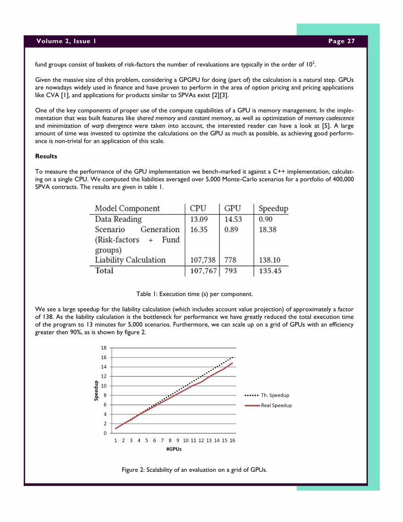
Page 27 Volume 2, Issue 1

fund groups consist of baskets of risk-factors the number of revaluations are typically in the order of 102.

Given the massive size of this problem, considering a GPGPU for doing (part of) the calculation is a natural step. GPUs

are nowadays widely used in finance and have proven to perform in the area of option pricing and pricing applications

like CVA [1], and applications for products similar to SPVAs exist [2][3].

One of the key components of proper use of the compute capabilities of a GPU is memory management. In the imple-

mentation that was built features like shared memory and constant memory, as well as optimization of memory coalescence

and minimization of warp divergence were taken into account, the interested reader can have a look at [5]. A large

amount of time was invested to optimize the calculations on the GPU as much as possible, as achieving good perform-

ance is non-trivial for an application of this scale.

Results

To measure the performance of the GPU implementation we bench-marked it against a C++ implementation, calculat-

ing on a single CPU. We computed the liabilities averaged over 5,000 Monte-Carlo scenarios for a portfolio of 400,000

SPVA contracts. The results are given in table 1.

Table 1: Execution time (s) per component.

We see a large speedup for the liability calculation (which includes account value projection) of approximately a factor

of 138. As the liability calculation is the bottleneck for performance we have greatly reduced the total execution time

of the program to 13 minutes for 5,000 scenarios. Furthermore, we can scale up on a grid of GPUs with an efficiency

greater then 90%, as is shown by figure 2.

Figure 2: Scalability of an evaluation on a grid of GPUs.

Page 28 TopQuants Newsletter

Upcoming Events

1. The next event is the 2014 TopQuants Spring workshop on May 28th. The event will be hosted by De

Nederlandsche Bank (DNB). The official invitation will be mailed soon and further details of the event will be posted in

due course on the TopQuants homepage .

2. The next issue of the TopQuants newsletter will follow in September 2014. Contributions for it are already

welcome. Kindly contact Aneesh Venkatraman, (newsletter@topquants.nl).

The computation time we achieved by using a GPU allows us to do intra-day valuations of a SPVA portfolio, as well as

computing Greeks and other sensitivities on the portfolio by using standardized bump-and-revalue techniques, reduc-

ing the average computation time for Greek calculations back from a scale of days to a scale of hours or minutes.

Acknowledgments

I would like to thank David Schrager and Andy Sklodowski from their support from the SPVA trading desk, further-

more I would like to thank my colleagues Drona Kandhai, Vladislav Sergeev and Tim Wood for their input for my

graduation thesis, where this article is based upon.

References

[1] V. Savickas et al., Super Fast Greeks: An Application to Counterparty Valuation Adjustments, Wilmott magazine, Vol.

2014, No. 69, 76-81, 2014.

[2] D. Bogg, Standard Life Canada adopts Aon Benfield's PathWise TM platform, April 27, 2011, source:

http://aon.mediaroom.com/index.php?s=25776&item=64210

[3] People Like VAs Like GPUs, Wilmott magazine, Vol. 2012, No. 60, 10-13, 2012.

[4] Algorithm of prefix sum scan using CUDA, http://http.developer.nvidia.com/GPUGems3/gpugems3_ch39.html

[5] CUDA Toolkit Documentation, http://docs.nvidia.com/cuda/