Embed Size (px)
Citation preview

IN DEGREE PROJECT MECHANICAL ENGINEERING,SECOND CYCLE, 30 CREDITS
, STOCKHOLM SWEDEN 2017
Topology Optimization in a Multi Disciplinary framework for a Turbine Rear Structure
TIMI OJO RUS
KTH ROYAL INSTITUTE OF TECHNOLOGYSCHOOL OF ENGINEERING SCIENCES

1
KTH Royal Institute of Technology
This thesis corresponds to the degree project of the Master’s programme in Aerospace Engineering trac
ight eight tr ct res at KTH Royal Institute of Technology.
The author takes full responsibility for opinions, conclusions and findings presented.
Industrial supervisor: Petter Andersson, GKN Aerospace Sweden
Academic supervisor: Per Wennhage, Royal Institute of Technology
Examiner: Per Wennhage, Royal Institute of Technology
Scope: 30 ECTS

2
KTH Royal Institute of Technology
Abstract
This thesis represents a research effort for the implementation of a structural optimization method known as
Topology Optimization (TO) in a multi disciplinary work environment. This application is tested in a platform
developed at GKN Aerospace Sweden named Engineering Workbench (EWB). The platform allows optimization of
aerospace structures for several disciplines including thermo-mechanics, aerodynamics and producibility. It utilizes
Knowledge-Based Engineering (KBE) tools to follow a Set-Based Concurrent Engineering (SBCE) and Design Of
Experiments (DOE) approach. Consequently, this enables obtaining results from different disciplines for a large
amount of design cases with limited human intervention.
The implementation is performed taking a Turbine Rear Structure (TRS) as a use case. This is a component from
a jet-engine which has been previously subject of study in EWB. The procedure already in use is extended in order
to obtain TO results for a desired number of design alternatives automatically. This extension is done while
considering the constraints imposed by the different disciplines. In addition, the positive contributions of the new
procedure to the structural design of components are analyzed.

3
KTH Royal Institute of Technology
Acknowledgments
I would like to thank the people at GKN in Trollhättan for their warm welcome and nice work environment.
They made me feel part of the team and kept me motivated throughout the whole project. Special gratitude to Petter
Andersson, who did not only provide me with this opportunity, but also guided me in the work and made my stay
much more enjoyable.
Great recognition to my family, who supported me during this time. Specially, thanks to my mother, who has
been always there for me, and to Charlie, who accompanied me during my studies but unfortunately could not be
there for the end.

4
KTH Royal Institute of Technology
List of Acronyms
AI = Artifitial Intelligence
CAA = Computer Aided Analysis
CAD = Computer Aided Design
CAE = Computer Aided Engineering
CAM = Computer Aided Manufacturing
DOE = Design Of Experiments
DRM = Design Research Methodology
DS-I = Descriptive Study-I
DS-II = Descriptive Study-II
EWB = Engineering Workbench
FE = Finite Element
GUI = Graphical User Interface
HM = HyperMesh
KBE = Knowledge-Based Engineering
KBS = Knowledge-Based System
KF = Knowledge Fusion
MDO = Multi-Disciplinary Optimization
MMG = Multi Model Generator
MOB = Mulltidisciplinary Optimization of a Blended wing body
MOO = Multi-objective Optimization
NLP = Nonlinear Programming
OO = Object-Oriented
OTM = Over-Turning Moment
PS = Prescriptive Study
RC = Research Clarification
RSM = Response Surface Methodology
SBCE = Set-Based Concurrent Engineering
SIMP = Solid Isotropic Microstructure with Penalization
SOO = Single-objective Optimization
TCL = Tool Command Language
TO = Topology Optimization
TRS = Turbine Rear Structure
VB = Visual Basic
XML = Extensive Markup Language

5
KTH Royal Institute of Technology
Table of Contents Abstract 2
Acknowledgments 3
List of Acronyms 4
I. Introduction 6
1. Research Questions 6
II. Frame of Reference 6
1. Theoretical Background 6
A. Multi-Disciplinary Optimization 6
B. Knowledge-Based Engineering 7
C. Set-Based Concurrent Engineering 8
D. Design Of Experiments 9
E. Topology Optimization 10
2. Industrial Context 11
A. GKN Aerospace Research Center Trollhättan 11
B. Software 12
C. Use case 13
III. Methodology 15
1. Design Research Methodology 15
2. Methodology implementation 16
A. Research Clarification 16
B. Descriptive Study I 16
C. Prescriptive Study 17
D. Descriptive Study II 17
IV. Findings 17
1. Description 17
A. Engineering Workbench 17
B. Topology Optimization 26
2. Implementation 30
A. Topology Optimization in Engineering Workbench 30
3. Validation 36
V. Discussion 39
VI. Conclusions 40
VII. Further Work 40
References 41
Appendix 43
Example I 43
Example II 45
Example III 47
List of Figures 50
6
KTH Royal Institute of Technology
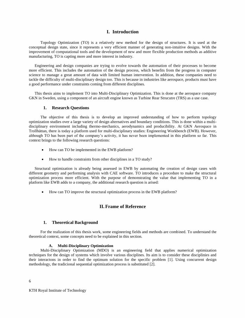
I. Introduction
Topology Optimization (TO) is a relatively new method for the design of structures. It is used at the
conceptual design state, since it represents a very efficient manner of generating non-intuitive designs. With the
improvement of computational tools and the development of new and more flexible production methods as additive
manufacturing, TO is capting more and more interest in industry.
Engineering and design companies are trying to evolve towards the automation of their processes to become
more efficient. This includes the automation of the design process, which benefits from the progress in computer
science to manage a great amount of data with limited human intervention. In addition, these companies need to
tackle the difficulty of multi-disciplinary design too. This is because in industries like aerospace, products must have
a good performance under constraints coming from different disciplines.
This thesis aims to implement TO into Multi-Disciplinary Optimization. This is done at the aerospace company
GKN in Sweden, using a component of an aircraft engine known as Turbine Rear Strucutre (TRS) as a use case.
1. Research Questions
The objective of this thesis is to develop an improved understanding of how to perform topology
optimization studies over a large variety of design alternatives and boundary conditions. This is done within a multi-
disciplinary environment including thermo-mechanics, aerodynamics and producibility. At GKN Aerospace in
Trollhättan, there is today a platform used for multi-disciplinary studies: Engineering Workbench (EWB). However,
although TO has been part of the company’s activity, it has never been implemented in this platform so far. This
context brings to the following research questions:
How can TO be implemented in the EWB platform?
How to handle constraints from other disciplines in a TO study?
Structural optimization is already being assessed in EWB by automating the creation of design cases with
different geometry and performing analysis with CAE software. TO introduces a procedure to make the structural
optimization process more efficient. With the purpose of demonstrating the value that implementing TO in a
platform like EWB adds to a company, the additional research question is arised:
How can TO improve the structural optimization process in the EWB platform?
II. Frame of Reference
1. Theoretical Background
For the realization of this thesis work, some engineering fields and methods are combined. To understand the
theoretical context, some concepts need to be explained in this section.
A. Multi-Disciplinary Optimization
Multi-Disciplinary Optimization (MDO) is an engineering field that applies numerical optimization
techniques for the design of systems which involve various disciplines. Its aim is to consider these disciplinies and
their interactons in order to find the optimum solution for the specific problem [1]. Using concurrent design
methodology, the tradicional sequential optimization process is substituted [2].

7
KTH Royal Institute of Technology
Traditionally in industry, MDO has found its application mostly at the detail design stage of a project, but its
used has progressively been moving towards the preliminary design stage. Thanks to the advantage provided by
advanced computational analysis tools, this more early utilization of MDO has the potential of reducing the time and
cost of the design cycle [3].
The beginning of MDO comes from its application in structural optimization and Schmit was the first using
Nonlinear Programming (N P) formalism in this discipline. N P’s general form lation is fo nd in ( 1 ).
( 1 )
In that formulation, f is the objective function to minimize, x is a vector composed of n design variables whose
values are between an upper and lower bound, p is a non-arbitrary vector affecting the system, and g an h are
constraints [3].
After a time, more disciplines apart of structural optimization were included in the optimization, as
aerodynamics, aircraft performance and propulsion in case of the aerospace industry. In this way, design variables
may be related to either one single discipline or to several ones at the same time. Moreover, within this frame, all
disciplines may have one common objective (Single-objective Optimization - SOO) or multiple objectives can come
from different disciplines (Multi-objective Optimization - MOO) [2].
MDO has the capacity of decomposing and coordinating the different disciplines so as to obtain a better design
overall in a relatively short time. To success in reaching this objective, special attention must be paid on choosing
the right organization of the disciplinary analysis models, approximation models and optimization software with
respect to the problem formulation [1].
The aerospace industry was the one beginning to use MDO, with applications like aircraft wing design, where
aerodynamics, structures and controls are strongly coupled disciplines. Furthermore, aerospace is still the industry
where MDO is most commonly used, but its application has been extended to others as well [4]. For instance, in the
automotive industry, MDO has been easier to apply in design phase, since the disciplines are less coupled than in
aerospace [3].
B. Knowledge-Based Engineering
Knowledge-Based Engineering (KBE) is an engineering method combining the disciplines object-oriented (OO)
programming, artificial intelligence (AI) and computed aided design (CAD) technologies. It constitutes a great
advanatage for computer-aided engineering (CAE), since it introduces customization for automated design. For
many years, this method has been only used by some highly competitive industries as aerospace and automotive [5].
From a managerial perspective, KBE give the opportunity to reduce product development time and engineering
costs. Moreover, from the point of view of knowledge management, KBE is a tool to keep knowledge of a company
and effectively use it in the future. On the other hand, engineers can make use of specific software tools, known as
KBE systems, to automatise repetitive and non-creative design tasks, and to aid the application of MDO during the
design process.
The relation between KBE and AI comes from the Knowledge Based Systems (KBS), computer applications
using stored knowledge for problem solving. They use reasoning mechanisms, which imply problem data and stored
knowledge, to provide solutions to the problems. This stored information, which is domain specific, is represented in
a symbolic way, most commonly in rules and frames forms. The rules form is constructed with the IF-THEN
structure, while the frames form uses attributes and/or operations related to an object and that appear described in

8
KTH Royal Institute of Technology
slots. The slots are simultaneously owning default values, pointer to other frames, or sets or fules and procedures
providing a value for the slot [5].
According to S. Quintana-Amate, P. Bermell-Garcia, A. Tiwari, C.J. Turner [6], after an experiment observing
engineers at work, 45% of their time was invested in the engineering design process and 21% in tasks related to
management of engineering knowledge. Consequently, it can be conlcuded that the engineering design process may
be represented as a group of knowledge intense activities.
The KBE systems combine the knowledge storing and representation ability of KBS with the potential of CAD
and Computer Aided Analysis (CAA) tools for geometry definition and data processing and computation. These
systems allow creating 3D designs, with the assistance of product and process-based data and relates them to rules,
requiremens, product attributes, features and even material selection and manufacturing capability [7]. They often
contain CAD system functionalities built-in, otherwise they are integrated to commertial CAD software.
Furthermore, it is possible to define on them the algorithms to implement analysis in external CAA tools. All this is
done in a rule-based design environment that save time from the engineering design process. Consequently, the use
of KBE applications is highly encouraged in case of design cases that are multidisciplinary, repetitive, highly rule-
driven or it requires geometry manipulation or product reconfiguration.
Within the aerospace industry, KBE applications have been used to produce Multi Model Generators (MMG).
They automatically create models of a specific family of products and the data needed for the analysis software
corresponding to the different disciplines under study.
A good example of MMG is found in the European project Mulltidisciplinary Optimization of a Blended wing
body (MOB), where more than 50 aircraft variants were studied with low and high precision analysis tools of
different disciplines by an automatic process and within only two days. If no KBE application would have been
used, this task would have lasted for months [5].
Another important feature available in KBE systems is the possibility of performing processes in batch mode,
hence greatly reducing the human intervention. This is very important when working with optimization [5].
C. Set-Based Concurrent Engineering
In product development business, the goal is to deliver products at a low cost earlier than the competitors.
Recycling reliable designs and knowledge and use them in new products is a way to reach this objective. In
industries where there is a constant demand for product evolution, reusing parts is not a good solution. Instead, a
better option is to reuse technologies, requirements and concepts from previous activities [8].
Set-Based Concurrent Engineering (SBCE) faces a product development problem taking into consideration a set
of alternative desing solutions from which knowledge is built along the way to obtain a more detailed product
specification. In the very last moment that a design decision is to be taken, the range of design solutions is narrowed
down systematically until one final solution is eventually selected. Solutions are discarded once there is enough
information to demonstrate that they are not as good as the others, that they are incompatible with coexisting partial
solutions or that their technology readiness level is too low. This gathered information is the one that is stored by a
company and reused for future products. An illustration of the SBCE method is shown in Figure 1.

9
KTH Royal Institute of Technology
Figure 1: SBCE method for an aircraft engine component development
This method can be compared to other common product development approaches as platform-based design and
point-based development. In the former, the main difference is that the range of options is not narrowed down to a
final design, but kept in order to produce a product family. The latter targets only a single solution that is iteratively
modified until requirements are fulfilled, hence, highly increasing lean times.
In Toyota’s prod ct development system, there is a special attention dedicated to system compatibility. They
study the interaction of every design in the system in which they are to be implemented before the completion of the
product. This compatibility study, which includes lean manufacturing too, greatly decreases the amount of design
modifications during the development process [9].
SBCE allows engineers and designers to work in parallel and relatively independently. Additionally, IT tools and
specific software have the chance to enhance collaboration and automation in the concurrent engineering work [10].
Lastly, a very relevant part of SBCE is the utilization of trade-off curves to map the design space. These curves
represent the relationship between two requirements mapped against each other according to the characteristics of all
possible solutions. Therefore, they allow to consider many design alternatives simultaneously [8].
D. Design Of Experiments
A Design Of Experiements (DOE) refers to a plan for experiements from which relevant data can be extracted
and then used to derive information through statistical analysis. It is a method which helps to find correlation
between a number of input variables and arbitrarily selected outcomes of the object under study. As a DOE allows
the modification of many variables simultaneously, statistics can also be used to study the influence of their
interactions on the ouput. The estimation of these dependencies should be achieved at minimial cost, which greatly
limits the number of samples [11]. Figure 2 illustrates a DOE, where output data is obtained from a system or
process after input data (or factors) is introduced. Unvoluntarily, some variables of which the experimentalist do not
have control are also introduced.

10
KTH Royal Institute of Technology
Figure 2: DOE structure [12]
To perform a DOE, the objectives of study must be formulated. These are the output parameters, which should
be able to be expressed quantitatively in order to take part in the statistical model. From them, a single response is to
be selected. This one has to be determinant for achieving the goal of the study, measurable and the product of a
single-value function.
Since the output is dependent of the input data, the right factors have to be taken in order to subtract appropriate
conclusions. All fundamental factors must be taken into consideration, as the error in the results increases for each
of those that are non included. However, the amount of factors should be as low as possible, since a higher number
requires a greater cost of the study in terms of time and resources. Moreover, the factors have to be under control of
the experimentalist either if they are qualitative or quantitative and they should be indepentend from other factors
[12].
Deciding on the right inputs requires of experience, enough information and expert knowledge. Commercial
software can be a help in the process [13].
The DOE method may be used to apply the Response Surface Methodology (RSM). This is used to model a
problem by representing the relationship between parameters and their responses, and optimize it. This optimization
process consists in moving from point to point in the response surfaces until the optimum is found.
E. Topology Optimization
TO is a mathematical method for structural optimization which is still relatively new. Even though its origin
dates from 1904, its main development came with the possibility of using powerful computers in the mid-80’s [14].
The method considers an initial design with a big structural domain refered as design space from which material
is removed after a number of iterations. After the optimization process, the design is supposed to have the best
material distribution according to the problem objective and constraints. The selection of the volume used as design
space depends on the interfacing surfaces with other components or on the requirements set by other disciplines as
aerodynamics or production. This volume should cover all space with likelihood of owning a load path, but it should
also be as small as possible to reduce the computational work time [15].
TO is commonly used upwards in the design process previous to other more detailed optimization methodologies
as shape or size optimization. It is a method with a lot of potential, as it can offer a view of how the design should
look like to be the most lightweight and still fulfil the structural requirements. However, the output of the
optimization cannot be directly taken as a final design for manufacturing. Instead, engineering expertise is needed to
build a final model from the interpretation of the results.
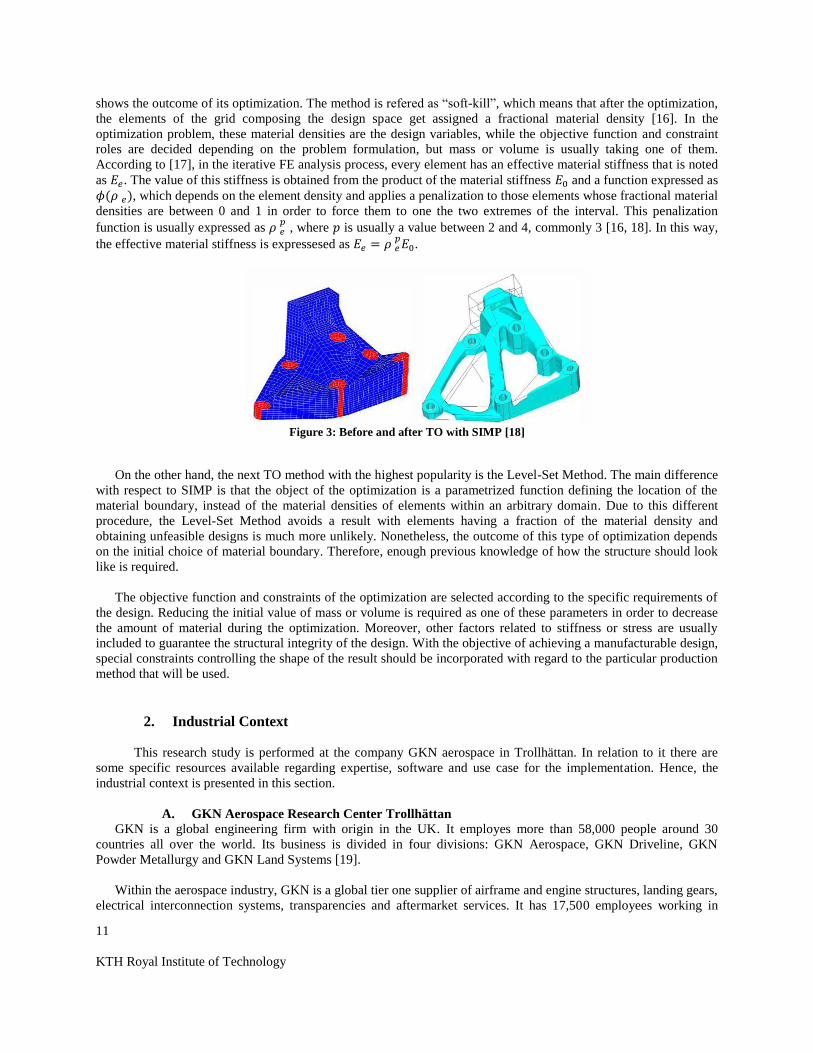
Within TO, there has been several methods under study. The most used one, which is found in most commercial
software, is called Solid Isotropic Microstructure with Penalization (SIMP). An example is illustrated in Figure 3,
where the left side shows the initial design of a compoenent whose design space appears in blue and the right side
11
KTH Royal Institute of Technology
shows the outcome of its optimization. The method is refered as “soft- ill”, which means that after the optimization,
the elements of the grid composing the design space get assigned a fractional material density [16]. In the
optimization problem, these material densities are the design variables, while the objective function and constraint
roles are decided depending on the problem formulation, but mass or volume is usually taking one of them.
According to [17], in the iterative FE analysis process, every element has an effective material stiffness that is noted
as . The value of this stiffness is obtained from the product of the material stiffness and a function expressed as
, which depends on the element density and applies a penalization to those elements whose fractional material
densities are between 0 and 1 in order to force them to one the two extremes of the interval. This penalization
function is usually expressed as , where is usually a value between 2 and 4, commonly 3 [16, 18]. In this way,
the effective material stiffness is expressesed as .
Figure 3: Before and after TO with SIMP [18]
On the other hand, the next TO method with the highest popularity is the Level-Set Method. The main difference
with respect to SIMP is that the object of the optimization is a parametrized function defining the location of the
material boundary, instead of the material densities of elements within an arbitrary domain. Due to this different
procedure, the Level-Set Method avoids a result with elements having a fraction of the material density and
obtaining unfeasible designs is much more unlikely. Nonetheless, the outcome of this type of optimization depends
on the initial choice of material boundary. Therefore, enough previous knowledge of how the structure should look
like is required.
The objective function and constraints of the optimization are selected according to the specific requirements of
the design. Reducing the initial value of mass or volume is required as one of these parameters in order to decrease
the amount of material during the optimization. Moreover, other factors related to stiffness or stress are usually
included to guarantee the structural integrity of the design. With the objective of achieving a manufacturable design,
special constraints controlling the shape of the result should be incorporated with regard to the particular production
method that will be used.
2. Industrial Context
This research study is performed at the company GKN aerospace in Trollhättan. In relation to it there are
some specific resources available regarding expertise, software and use case for the implementation. Hence, the
industrial context is presented in this section.
A. GKN Aerospace Research Center Trollhättan
GKN is a global engineering firm with origin in the UK. It employes more than 58,000 people around 30
countries all over the world. Its business is divided in four divisions: GKN Aerospace, GKN Driveline, GKN
Powder Metallurgy and GKN Land Systems [19].
Within the aerospace industry, GKN is a global tier one supplier of airframe and engine structures, landing gears,
electrical interconnection systems, transparencies and aftermarket services. It has 17,500 employees working in

12
KTH Royal Institute of Technology
more than 55 manufacturing locations in 14 countries worldwide. At GKN, they maintain a strong cooperation with
universities and research centers in order to keep the lead in new technology development for lower costs weight
and emissions of aircrafts. Some recent examples of vehicles using GKN products are Airbus A350XWB, A380,
Boeing 737 and Ariane 5 [20].
In Sweden, GKN has two location belonging to the sub-division GKN Aerospace Engine Systems since Volvo
Aero was boutght in 2012. There, the work is mostly dedicated to develop composites and advanced metallic
technologies for jet-engines, and to nozzles and turbines for the European space program [21, 22].
The headquarters of GKN Aerospace are located in Trollhättan, Sweden. The R&T centre in this location
currently employes more than 70 people and is divided in three departments that cooperate one to each other. The
work performed during this thesis takes place at the department Design Engineering, focus in concept design and
definition of new technology in aero engine modules, and in developing new product concepts and implementing
new design tools.
B. Software
The software used during this thesis is described for a better comprehension of the subsequently development of
work.
Siemens NX
Siemens NX is a CAD/CAM/CAE software package developed by Siemens PLM Software. It allows
collaborative design engineering work thanks to its tight integrations with Teamcenter, a product lifecycle
management platform [23].
An important advantage that this software offers to the development of this thesis work is the possibility of using
customization and programming tools, making it a KBE system. Knowledge Fusion is an interpreted, object-oriented
language allowing to work on a design for automation environment [24], where DOE can be applied with very
efficient results.
HyperMesh
HyperMesh is a high-performance finite element pre- and post-processor belonging to HyperWorks, a CAE
simulation platform developed by Altair Engineering. It supports direct use of the CAD geometry produced in
Siemens NX providing robust interoperability, as with the extraction of CAD metadata. This software also contains
a big number of automation tools, including geometry corrections and meshing. In addition, it has an easy to utilize
user-interface, but it also gives the possibility of customization by writing TCL (Tool Command Language) scripts.
The implementation of these scripts gives the chance to automate the pre-processing of FE models, which can
subsequently be exported in several kinds of formats for its analysis in different solvers [18].
OptiStruct
OptiStruct, within the HyperWorks package, is a finite element solver for linear and non-linear structural design
problems of a wide range, from preliminary to detailed design. It was mainly developed for optimization purposes,
being Topology Optimization one of the possibilities. The main TO method in OptiStruct is SIMP, and it is the one
used in the development of this thesis. This solver requires a file of .fem format to be executed and it produces as
output log and result visualization files, among others [18].
HyperView
HyperView, also from HyperWorks, is a complete post-processing and visualization environment for different
studies, including finite element analysis. It can read the visualization files created in OptiStruct and show the results
of the analysis with 3D graphics [18].
13
KTH Royal Institute of Technology
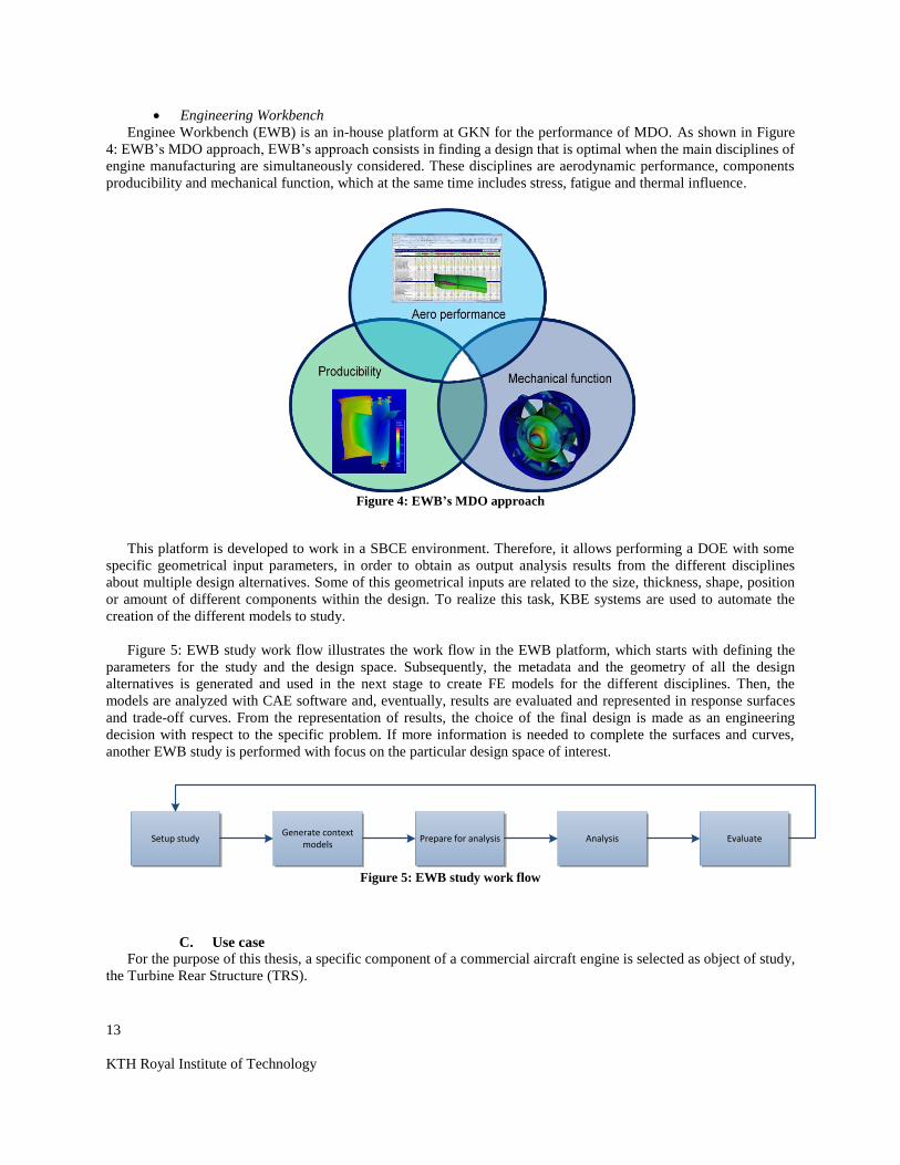
Engineering Workbench
Enginee Workbench (EWB) is an in-house platform at GKN for the performance of MDO. As shown in Figure
4: EWB’s MDO approach, EWB’s approach consists in finding a design that is optimal when the main disciplines of
engine manufacturing are simultaneously considered. These disciplines are aerodynamic performance, components
producibility and mechanical function, which at the same time includes stress, fatigue and thermal influence.
Figure 4: EWB’s MDO approach
This platform is developed to work in a SBCE environment. Therefore, it allows performing a DOE with some
specific geometrical input parameters, in order to obtain as output analysis results from the different disciplines
about multiple design alternatives. Some of this geometrical inputs are related to the size, thickness, shape, position
or amount of different components within the design. To realize this task, KBE systems are used to automate the
creation of the different models to study.
Figure 5: EWB study work flow illustrates the work flow in the EWB platform, which starts with defining the
parameters for the study and the design space. Subsequently, the metadata and the geometry of all the design
alternatives is generated and used in the next stage to create FE models for the different disciplines. Then, the
models are analyzed with CAE software and, eventually, results are evaluated and represented in response surfaces
and trade-off curves. From the representation of results, the choice of the final design is made as an engineering
decision with respect to the specific problem. If more information is needed to complete the surfaces and curves,
another EWB study is performed with focus on the particular design space of interest.
Figure 5: EWB study work flow
C. Use case
For the purpose of this thesis, a specific component of a commercial aircraft engine is selected as object of study,
the Turbine Rear Structure (TRS).
Setup study Generate context
modelsPrepare for analysis Analysis Evaluate
Setting up the EWB environment
Perform EWB MDO study
List of documents

14
KTH Royal Institute of Technology
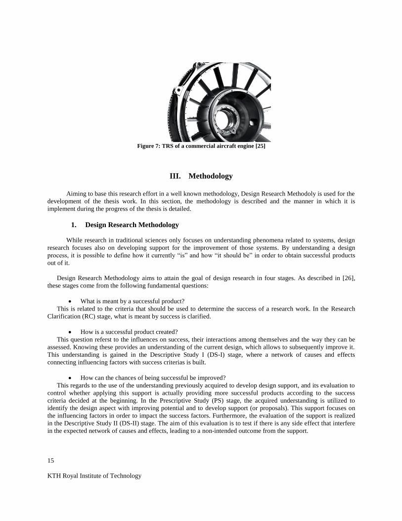
As illustrated in Figure 6: Commercial aircraft engine with the TRS highlighted and Figure 7: TRS of a
commercial aircraft engine , this part is located at the engine exit, it supports the back end of the low-pressure
turbine rotor and contains the rear engine mounts. It incorporates exit guide vains which carry the load to support the
bearing chamber, whose roller bearings transfer radial load. These vanes contain instrumentation cables and oil and
air pipes for lubrication and cooling. The shape of these vains is simplier than those of the turbine stators because
they need to provide less turning of the airflow. However, a proper aerodynamic design is essential for a good
performance of the engine.
Furthermore, the rear bearing chamber needs to allow a protected environment for the lower-pressure shaft rear
roller bearings and the low-pressure turbine over-speed probe.
Regarding production, since the TRS is exposed to high temperatures at the end of the exit of approximately
600ºC, super-alloys are required as materials for manufacturing. Usually, the chosen material is a nickel-based alloy
and the productions method varies from full casting to fabrication. On the ther hand, the bearing chamber housing is
made of either cast steel alloy or cast nickel alloy [25].
The aim of performing a topology optimization study of this component is to obtain the most lightweight design
under the constraints presented by the structural, thermal and aerodynamic requirements, and the state-of-the-art
manufacturing methods.
Figure 6: Commercial aircraft engine with the TRS highlighted [25]
15
KTH Royal Institute of Technology
Figure 7: TRS of a commercial aircraft engine [25]
III. Methodology
Aiming to base this research effort in a well known methodology, Design Research Methodoly is used for the
development of the thesis work. In this section, the methodology is described and the manner in which it is
implement during the progress of the thesis is detailed.
1. Design Research Methodology
While research in traditional sciences only focuses on understanding phenomena related to systems, design
research focuses also on developing support for the improvement of those systems. By understanding a design
process, it is possible to define ho it c rrently “is” and ho “it sho ld be” in order to obtain successful products
out of it.
Design Research Methodology aims to attain the goal of design research in four stages. As described in [26],
these stages come from the following fundamental questions:
What is meant by a successful product?
This is related to the criteria that should be used to determine the success of a research work. In the Research
Clarification (RC) stage, what is meant by success is clarified.
How is a successful product created?
This question referst to the influences on success, their interactions among themselves and the way they can be
assessed. Knowing these provides an understanding of the current design, which allows to subsequently improve it.
This understanding is gained in the Descriptive Study I (DS-I) stage, where a network of causes and effects
connecting influencing factors with success criterias is built.
How can the chances of being successful be improved?
This regards to the use of the understanding previously acquired to develop design support, and its evaluation to
control whether applying this support is actually providing more successful products according to the success
criteria decided at the beginning. In the Prescriptive Study (PS) stage, the acquired understanding is utilized to
identify the design aspect with improving potential and to develop support (or proposals). This support focuses on
the influencing factors in order to impact the success factors. Furthermore, the evaluation of the support is realized
in the Descriptive Study II (DS-II) stage. The aim of this evaluation is to test if there is any side effect that interfere
in the expected network of causes and effects, leading to a non-intended outcome from the support.

16
KTH Royal Institute of Technology
If eventually, the results are not acceptable, the support should be modified in the PS stage. In case of the result
not being acceptable yet, the understanding of success and design phenomena should be improved at the DS-I or RC
stage.
A diagram explaining the stages of the Design Research Methodolody appears in Figure 8.
Figure 8: Stages in Design Research Methodology [26]
2. Methodology implementation
A. Research Clarification
As previously mentioned, the aim of this thesis work consists on developing an improved knowledge of
Topology Optimization in EWB, the MDO platform at GKN. For this, the work is developed over a use case that is
represented by the Turbine Rear Structure of a jet-engine, which has already been object of study within EWB. With
the objective of defining a success criteria, the TO study to implement is assessed under the same constraints as the
ones used for previous structural analysis. Moreover, the main load cases, including load magnitudes, are those that
have been also used in these previous studies, that are easier to implement in TO and whose results are easier to
evaluate compared to those of TO. These load cases are related to linear static studies of force and bending moment,
and they are known as x-stiffness and Over-Turning Moment (OTM) respectively. The results provided from the TO
implementation in EWB is a certain number of design cases with its optimized material distribution and the
corresponding stress and displacement distribution. These results can be compared to their equivalents from the
other studies in order to estimate the success of the solution.
In addition, since the work is performed within EWB, the TO study process should be as automatic as for the
other studies performed in the same platform. The amount of human interventions from the Set up stage to the
Evaluation can be compared to the one of previous structural analysis as measure of success.
B. Descriptive Study I
Since TO has been used at GKN previously, but it has never been implemented in EWB before, it is necessary to
start investigating separately the work flow in EWB and the implementation of TO in single design studies. Once a
good understading has been reached about these two, the possibility of combining them into a single system can be
assessed in order to create an engineering practice.
On the one hand, the understanding of the EWB work flow starts with an introduction from the thesis supervisor,
who is also the technology leader in MDO. The supervisor gives an explanation about the general process,
introduces the needed software, the working files and directories in the computer, and provides the internal

17
KTH Royal Institute of Technology
documents describing in more detail the multiple steps involved. Thereafter, independent review of these documents
is done to obtain a deeper insight. The latter is complemented with the attendance to several presentations about
EWB directed to both internal and external audience, and to meetings of teams working in the development of this
platform. Furthermore, in meetings with experts in the different stages of the process, the understanding of more
detailed information is reached through discussions and test runs for demonstration. Lastly, independent test runs are
executed to corroborate the acquired undertsanding.
On the other hand, the means to understand the work in TO with the chosen software begins with literature
review about the theory behind it and about previous applications on projects. Much valuable knowledge is also
obtained through the tutorials and the user guide provided in the HyperWorks package. Moreover, discussions with
colleagues having worked on the topic for many years provided very relevant input. These colleagues also shared
some of their documents from previous projects as examples. Additionally, far from an automation environment,
simple TO studies are carried out using the Graphical User Interface (GUI) in the used software in order to support
the understanding of the method.
The understanding reached in this stage is described in detail in section IV.1.
C. Prescriptive Study
The implementation of TO in the EWB platform is mainly based on two considerations. First is having a model
in which TO can be applied and which is adapted to the automation environment of EWB. Second consideration is
dividing the TO process in the different stages that compose the work flow of the platform and making all these
steps automatic. In order to do that, the work performed in the various software applications cannot be done through
the GUI, but running scripts written in the language recognized by each software. These scripts are obtained by
modifying existing ones or creating new ones. Therefore, an intense study of the current scripts and the software
guides is required. The motivation for such considerations is that TO should take part in EWB as one more
discipline study, requiring the minimum amount of additional inputs and providing results in parallel to the other
studies for global evaluation of the design. This method should allow meeting the success criteria defined before.
The development of the previous method is elaborated in section IV.2.
D. Descriptive Study II
Aiming to assess the developed method, this is regarded with respect to the success criteria defined in the RC
stage. A way to scrutinize the effectiveness of the implementation of TO for the linear studies mentioned formerly is
comparing the results coming from test runs of the new process to the ones obtained from previous structural
analysis in EWB. The stress and displacement distributions obtained on the new topology should be similar enough
to the other ones in order to validate the success of the implementation. The magnitude of the difference between the
results demonstrate the reliability of the new method and hence, the extent until which it can be used in the design
process of new products. Conjointly, in order to examine the automation level of the solution, several TO test runs
can be executed for a number of design cases. Then, other EWB studies for the same design cases can be performed
too, and the amount of times that human intervention is needed during the whole process can be compared.
IV. Findings
1. Description
A. Engineering Workbench
As explained before in this text, the EWB work flow is divided in several stages. Each stage is important for the
implementation of multi-disciplinary studies. Therefore, they are detailed below for the application on the TRS.
a) Setup study
In this stage, the purpose of the study and the expected results are defined. Accordingly, the input files for all
disciplines involved in the study are set. The current available disciplines are Product definition, CAD, Mesh, Stress
and Fatigue, Thermodinamics, Aerodynamics and Producibility.

18
KTH Royal Institute of Technology
The CAD assembly for the TRS is created in Siemens NX as a shell model and is shown in Figure 9. The KBE
tools mentioned in II.2.B are integrated in this software and they allow introducing a considerable amount of
information in the model automatically. This information includes geometrical data, materials and reference names
to divide the model in compoonents. Using the KBE tools, features defined in the model can be assigned to rules or
be linked to data in an Excel file.
Figure 9: CAD assembly of TRS
When setting up the targeted study, the design configuration regarding the TRS model and the baseline
parameters is selected. The design features that will not change for the different design cases are defined with fixed
values. Moreover, the baseline values for the parameters of the design that are modified during the study, referred to
as design variables, are also specified. Examples of these geometrical inputs, of both fixed or changing values, can
be number of vanes, sheet thicknesses, bearing flange position or geometry of the outer case. All these inputs are
stored in an Excel file as Geometrical Expressions and Face Attributes. Every input is introduced in a table with its
required information, as its name and value (number or string). The values of this table are linked to the geometrical
features in the CAD model by the KBE tools.
In order to set up a DOE, commercial software is used to generate a distribution of values for the design
variables that eventually creates a uniform space of design case alternatives. This is done by selecting an upper and
lower value for the variance of the distribution and then, filling the design space using a space-filler methodology
like the latin hypercube, described in [11]. Every design case of the study and their corresponding design variables
are listed in a table and stored in the same Excel file as before. This information is also linked to the CAD model,
using the KBE tools.
The faces of the model are divided in different components and they are assigned their own Face Attribute input
in the Excel file. When defining this attribute, component and material names are introduced in the table together
with the thicknesses. This allows including this information in the CAD model.

19
KTH Royal Institute of Technology
Similarly as with the Face Attributes, Edge Attributes and Point Attributes are defined in the same Excel file and
linked to existing edges and points in the CAD model. This is to define the edges that represent welds and the mass
center points for application of loads, which are used later in the process.
Lastly, special geometrical information is required from aerodynamic studies to define the profile of the vanes.
An additional attribute is introduced in the Excel file and a link pointing to an external file is included. This
procedure connects automatically the geometry dictated by aerodynamic analysis to the CAD model.
The flowchart in Figure 10 represents the connections between the DOE Excel file and the CAD model as it has
been described above.
Figure 10: Connections between DOE Excel file and CAD model
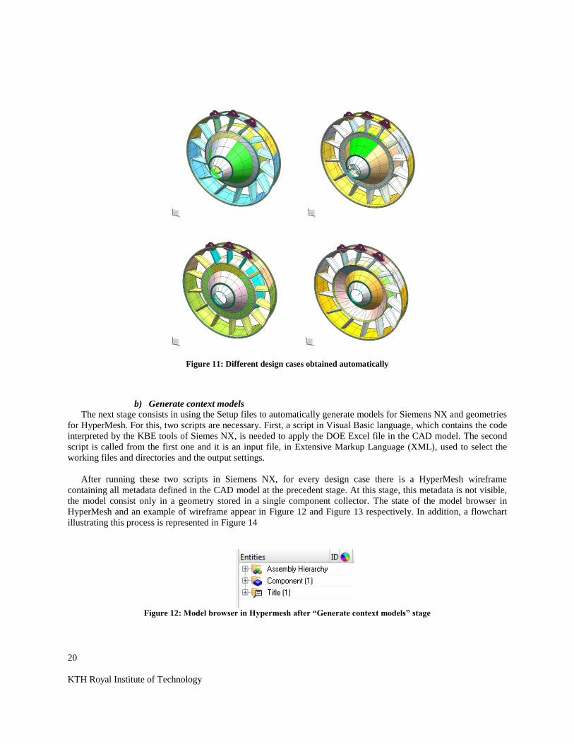
Once all of the above is implemented, all design cases can be automatically obtained from the original CAD
assembly by selecting it from the settings in Siemens NX. An example of how the geometry can be variated is
shown in Figure 11.
20
KTH Royal Institute of Technology
Figure 11: Different design cases obtained automatically
b) Generate context models
The next stage consists in using the Setup files to automatically generate models for Siemens NX and geometries
for HyperMesh. For this, two scripts are necessary. First, a script in Visual Basic language, which contains the code
interpreted by the KBE tools of Siemes NX, is needed to apply the DOE Excel file in the CAD model. The second
script is called from the first one and it is an input file, in Extensive Markup Language (XML), used to select the
working files and directories and the output settings.
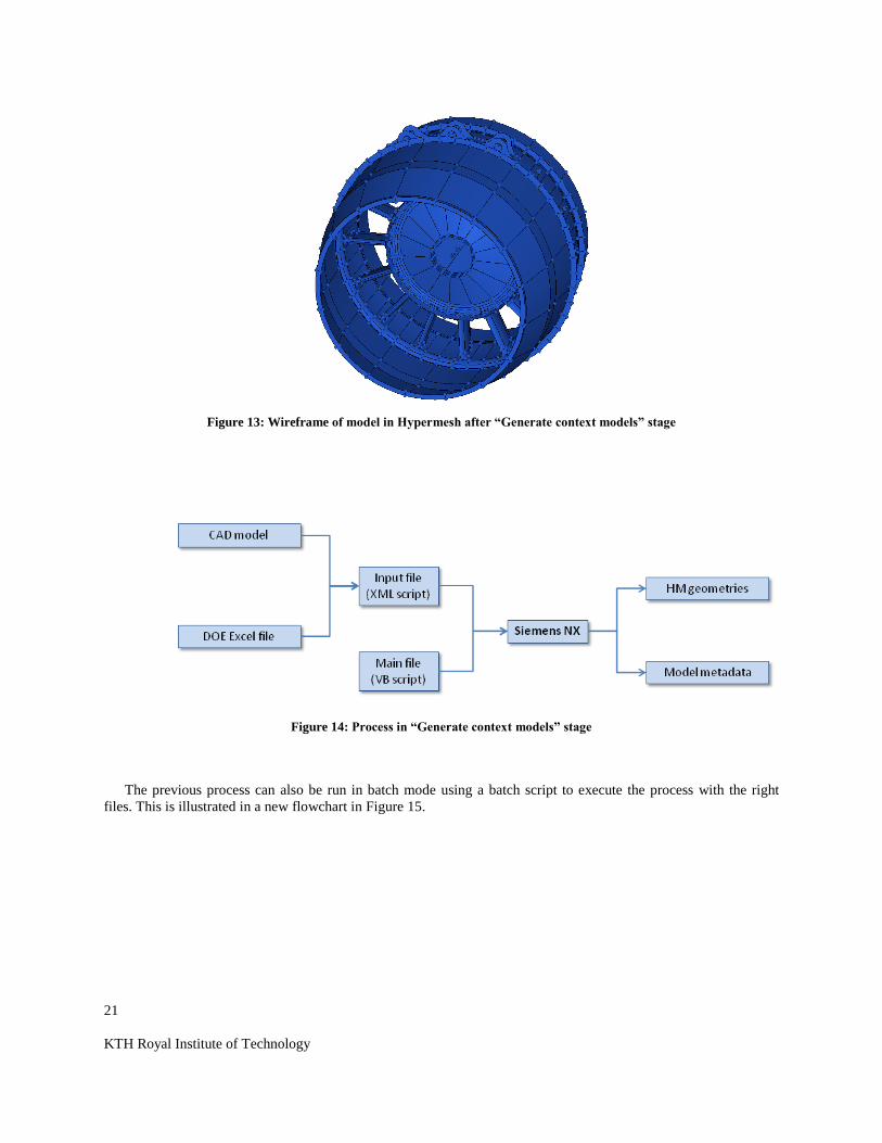
After running these two scripts in Siemens NX, for every design case there is a HyperMesh wireframe
containing all metadata defined in the CAD model at the precedent stage. At this stage, this metadata is not visible,
the model consist only in a geometry stored in a single component collector. The state of the model browser in
HyperMesh and an example of wireframe appear in Figure 12 and Figure 13 respectively. In addition, a flowchart
illustrating this process is represented in Figure 14
Figure 12: Model browser in Hypermesh after “Generate context models” stage
21
KTH Royal Institute of Technology
Figure 13: Wireframe of model in Hypermesh after “Generate context models” stage
Figure 14: Process in “Generate context models” stage
The previous process can also be run in batch mode using a batch script to execute the process with the right
files. This is illustrated in a new flowchart in Figure 15.

22
KTH Royal Institute of Technology
Figure 15: Process in “Generate context models” stage when run in batch mode
c) Prepare for analysis
The preparation for the analysis involves creating an FE model from the HyperMesh wireframe and the metadata
coming from the CAD model. Many operations have to be performed in this stage automatically. Therefore, a script
in TCL format should be written and run in HyperMesh. The more relevant operations for the study of this thesis are
as follow:
Execute metadata.
The first operation to command in the script is interpreting the metadata transferred from the CAD model so
it can be used to perform the rest of the operations.
Divide faces and points of geometry in component collectors.
According to the names associated to the faces and points of the geometry in the first stage, component
collectors are created for each of them.
Create property collectors.
For each component containing a face, a property collector is created and connected to it. Metadata is read
to assign a thickness value to the component and store it in the property. These thickness values are those
defined in the Excel file. Moreover, a card image PSHELL is defined so the component can be analyzed as a
shell in the OptiStruct solver. For structural analysis in another solver, like Ansys, the card image has to be
different.
Create material collectors.
For each component containing a face, a material collector is created and connected to it and its property.
The materials are those defined in the Excel file.
Mesh surfaces.
Every surface of the geometry is meshed using an automatic mesh tool in HyperMesh. Two options are
provided, one providing a fast mesh and another one which runs for longer time but provides better mesh
quality. The element size and type is defined in the script.
Create interpolation constraint elements.
The points of the model are used as center mass points for load application. Interpolation constraint
elements are created to be used to transfer loads and moments from the points to the faces. For OptiStruct,
RBE3 elements are used.
Creat set collectors for weld interfaces and thermal zones.
Edges and faces that were tagged in the first stage are gathered in set collectors that are used for weld life
and thermal analysis, respectively.

23
KTH Royal Institute of Technology
Save and export model.
At the end of all operations, the FE model is complete and can be saved. With the purpose of running
structural analysis in other softwares, like Ansys, the model is exported in the corresponding format.
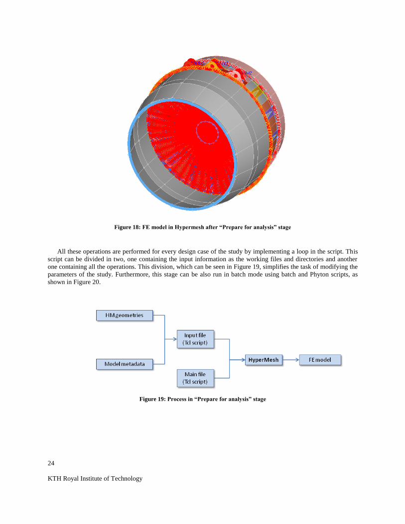
The new state of the model browser at the end of this stage appears in Figure 16 and an example of the information
contained in a property collector is found in Figure 17. Moreover, the FE model generated at this stage is illustrated
in Figure 18.
Figure 16: Model browser in Hypermesh after “Prepare for analysis” stage
Figure 17: Property collector information in HyperMesh
24
KTH Royal Institute of Technology
Figure 18: FE model in Hypermesh after “Prepare for analysis” stage
All these operations are performed for every design case of the study by implementing a loop in the script. This
script can be divided in two, one containing the input information as the working files and directories and another
one containing all the operations. This division, which can be seen in Figure 19, simplifies the task of modifying the
parameters of the study. Furthermore, this stage can be also run in batch mode using batch and Phyton scripts, as
shown in Figure 20.
Figure 19: Process in “Prepare for analysis” stage

25
KTH Royal Institute of Technology
Figure 20: Process in “Prepare for analysis” stage when run in batch mode
d) Analysis
Once the FE model is ready in the format required by the different solvers involved in the study, the analysis can
be run for all design cases. In the case of stress and fatigue analysis, Ansys is the solver used. OptiStruct is not used
in EWB yet, therefore, there is not very useful knowledge that can be used from this stage.
e) Evaluate
Results of the analysis from all disciplines are stored and organized in different formats of data representation.
An example of contour plots created for a number of design cases after a structural analysis appears in Figure 21.
Figure 21: Structural analysis results obtained in Ansys for a number of design cases
Since neither OptiStruct or TO are part of the EWB platform at this moment, there is no relevant information to
substract from this stage of the process.

26
KTH Royal Institute of Technology
B. Topology Optimization
a) Preparing the model
As mentioned in II.1.E, TO requires the definition of a design space which contains all the design variables. This
design space can be a sheet or a solid body, depending on the component and target of the study. In general, as TO
of sheet bodies does not account for changes through the thickness, when a design wants to be explored with the
fewest constraints as possible, the design space is a 3D domain. However, if the model contains areas that are not
part of the design space, they may be still considered as sheet bodies, making the model hybrid. The fact of working
with sheet bodies may represent an advantage when meshing the body, since they are easier to mesh than solid
bodies.
Another important factor to consider in the geometry modeling stage is the division of the whole model in
bodies. This process, when performed in the CAD model, saves time in manual geometry corrections afterwards. If
the CAD model has properly selected division boundaries, when the geometry is imported in HyperMesh, automatic
meshing tools can be directly applied. Otherwise, body divisions have to be corrected, or more time have to be
invested in obtaining a good mesh. Both activities decrease the automation potential of the meshing operation.
When focusing on the creation of the FE model, there are four main points to take into consideration:
Mesh connectivity node-to-node:
To obtain good results from the simulation, a right connectivity has to be assured between nodes. Special
attention must be paid in the interface between different bodies, since automatic meshing tools do not
always guarantee a proper connection. Figure 22 shows an example of bad connectivity. As said
previously, a good division of the geometry prior to meshing helps the software to provide the required
connectivity.
Figure 22: Bad connectivity between mesh in two adyacent components
Element size
The size of the mesh elements has a considerable effect in TO. Firstly, a coarse mesh requires much less
computation time than a fine one, due to the lower amount of design variables to consider in the
optimization. Secondly, TO is affected by mesh-dependency. Since the physical description of the problem
is ill-posed, a finer mesh provides solutions with thiner members, risking of being a non-manufacturable
solution [17]. On the other hand, coarser mesh loses resolution in the results.
Element order
Using elements of first order instead of second order ones greatly reduces the simulation time. Nevertheless,
this makes the analysis less accurate, giving rise to a problem known as checkerboarding. This
27
KTH Royal Institute of Technology
phenomenom, where the optimized structure alternates solid and void elements, is a consequence of the load
transfer between elements, which gives to the model a higher stiffness than it really has, affecting the
continuity of element density. One of the best approaches to solve this problem is known as node-based
formulation, which aims to obtain a continuous density field [17].
Element quality
In a stess analysis, the quality of the elements has to be over a threshold that ensures accurate results. In TO,
the requirements for accuracy are not as high and the threshold is much more tolerant. OptiStruct has a
quality threshold that depends of the feasibility of the mathematical calculations.
b) Preparing optimization
Regarding the type of studies that can be part of TO, the linear static analysis are the most common and easy to
evaluate, hence they have been the focus of this thesis work. However, OptiStruct presents the possibility of
introducing heat transfer, fatigue and dynamic/non-linear analysis as well.
For linear static studies, forces or bending moments and constraints have to be defined. Every combination
creates a load case that can be analysed individually or in combination with the others.
When it is time to set up the optimization, the parameters of interest have to be selected as responses. From
them, the objective and the constraints of the optimization are defined. They may be related to independent load
cases or to all of them simultaneously. The main responses to obtain from a linear static analysis are the following:
Mass or volume fraction
The mass or the volume of the structure are the most important responses of TO. It is a response that takes
into account all load cases. It may be more practicle to measure it as a fraction, so it measures the lost of
material of the whole structure or of selected components with a value between 0 and 1. The volume
fraction considers the proportion between the volume of the design space before and after the optimization,
while the mass fraction also takes the non-design space into account.
Weighted compliance
The compliance is the inverse of the stiffness, hence the lower the compliance, the higher the stiffness. The
weighted compliance is the weighted sum of the compliance of all load cases on the whole structure.
Therefore, it is possible to choose the load cases that are more important for the optimization.
Static displacement
The displacement of arbitrarily selected nodes can be measured for one load case.
Static stress (DRESP1)
It is possible to measure the stress in selected components or elements for the combination of load cases.
This stress can be Von Misses, normal, shear or principal, and it is calculated according to the Stress
NORM method, described in [18].
Static stress (DTPL)
There is another type of stress response that can only be used as constraint. It is related to the whole
structure and measures only the Von Misses stress.
From all these responses, those related to stresses present some complications and there is not much information
in the literature about how to handle them. One of the problems is that the stress response is only global, thus when
it is used as constraint, the local stresses are not controlled and have to be studied in a separate size or shape
optimization. Another difficulty is associated to the elements affected by the constraint. Since eliminating an
element also supresses its constraint, the constraint should not be applied only in the domain of the design space.
The topology solutions are different depending on which responses are used as objective function and as
constraints. This selection affects the topology result and the computation time. As seen in [15, 27, 28] and in
company projects, some common alternatives are the following:

28
KTH Royal Institute of Technology
Objective function: minimize compliance / Constraint: maximum volume fraction
It is one of the most common alternatives in literature. It helps to optimize for stiffness and to identify load
paths in the structure. In order to obtain the lowest possible weight of the structure, the optimization has to
be repeated while lowering the constraint iteratively.
Objective function: minimize volume fraction / Constraint: maximum compliance
It is not common in literature. It provides the minimum weight directly, but it requires setting a constraint
for the compliance, which is not obvious.
Objective function: minimize volume fraction / Constraint: maximum displacement
A very common procedure that provides directly the lowest weight, but which requires a good knowledge of
the structure. This is because the nodes where the displacement constraint is applied are arbitrarily selected
and the more nodes are selected, the more time is required to run the optimization.
Objective function: minimize volume fraction / Constraint: maximum displacement and stress
This is similar to the previous alternative, but it includes a stress constraint to ensure the strength of the
structure.
In addition to the previous parameters of the optimization, it is possible to include constraints that help obtaining
a topology solution that can be manufactured by the methods available. The manufacturing constraints currently
available in OptiStruct [18] are:
Minimum member size control
This constraint defines the minimum diameter of the members of the resultant topology. It is used to avoid
too thin structural elements, but attention must be paid in not decreasing too much the flexibility of the
design. Therefore, a diameter of between 3 and 12 times the average element size is recommended. An
example to show the effect of this constraint is found in Figure 23.
Figure 23: TO result without manufacturing constraints (left) and with minimum member size control (right)
Draw direction
This constraint is made when the intended production method is casting. A draw direction is imposed so the
structure cavities are lined up with the sliding direction of the die. There are two options available,
depending if the intention is to use a single die or two dies. Moreover, there is also an option to avoid
through-holes and another one to create a sheet of uniform thickness as optimized shape.
Extrusion
When it is desired to have a structure with constant cross-section over a specific path, this constraint can be
applied. Whether the cross-sections twist or not along the path can be defined in the settings.
Pattern repetition
It is a technique that link structural components so they have a similar shape. A scale factor determines the
relation of one to each other.
Symmetry
This constraint gives the possibility of forcing the layout of the structure to be symmetric with respect to a
plane or to a central axis.
Uniform element density

29
KTH Royal Institute of Technology
Lastly, it is also possible to maintain the shame element density for defined components.
Some of those constraints can be combined together in order to adapt TO to the desired manufacturing method.
c) Interpreting results
After running the optimization in OptiStruct, the results can be visualized in HyperView. The optimized shape of
the structure can be visualized for every iteration with ISO and contour plots. In the ISO plot, it is possible to show
only the elements of the structure that are above a specific threshold. By adding a contour plot, colors identify
elements that have higher density than others. This is illustrated in Figure 24, where the ISO plots are visualized for
element density thresholds 0.2, 0.5 and 0.8.
Figure 24: ISO plot with element density thresholds 0.2 (up and left), and combination of ISO and contour plots with
element density thresholds 0.2 (up and right), 0.5 (down and left) and 0.8 (down and right)
HyperView also provides the stress and displacement distribution in the structure for every load case at the first
and last iterations. This is useful to examine the validity of the solution.

30
KTH Royal Institute of Technology
In addition, looking into the log file created by OptiStruct it is possible to obtain the value that the responses
have and the total mass of the model after every iteration.
Finally, from the topologies it is possible to extract that the elements with higher density are more important for
the structure than those with lower density. Therefore, the results need to be interpreted with engineering judgement
and experience in order to realize modifications in the initial design. In case of planning to create a new design as
faithful as possible to the optimized shape, the HyperMesh tool OSSmooth allows to export the geometry or a FE
model of the shape at the desired density threshold. Consequently, it is possible to work on that model and to
prepare it for a new analysis that will confirm its validity.
2. Implementation
A. Topology Optimization in Engineering Workbench
Once the EWB process and the TO methodology are understood in detail, it is possible to integrate the latter into
the former in every of the stages described in IV.1.A.
a) Setup study
First of all, it is necessary to modify the current CAD shell model in order to have a volume domain used as
design space, where TO is applied. As subject of study for this thesis work, it is decided to work on the hub of the
TRS. Hence, a solid version of the hub is created inside the whole TRS assembly, substituting the parts
corresponding to the current design. The new assembly is illustrated in Figure 25.
Figure 25: CAD assembly of TRS with solid hub
With the purpose of automating the choice between performing a regular analysis with a full shell model or
performing a TO with this hybrid model, KBE tools can be used. A rule is created to select either shell hub or solid
hub. Then, in the DOE Excel file a new Expression can be added to choose the baseline version of the hub and if
desired, the choice can also be added as design variable in the DOE study. The two alternatives are shown in Figure
26.

31
KTH Royal Institute of Technology
Figure 26: Section of the two hub alternatives for the TRS model
It is very important to check that the modification of the assembly to include the solid hub is robust enough to
work with all geometry combinations of the DOE.
b) Generate context models
To create the multiple geometries with metadata, no major changes to the original process are needed. Once the
new DOE Excel file is obtained from the previous stage, just the new directories and working files have to be
referenced in the XML input file, while the Visual Basic script does not need any modification.
c) Prepare for analysis
The next stage, consisting in generating the FE models, requires writing a great amount of new code to the
precedent TCL scripts. The reason for this is that using a hybrid model implies adding many new operations, from
which the following ones are highlighted:
Organize solids in components
Since the original script uses metadata in faces to split the model in components, a code must be written to
create components for solids using their metadata.
Remove solid and substitute by surfaces
Aiming to keep as much of the original code as possible, the solid geometries are substituted by its surfaces
in the same component. Consequently, most of the operations already defined for surfaces can still be used.
Equivalence geometry
Although already existing in the previous code, this operation is highlighted here for its importance to get a
proper mesh. Equivalencing the geometry of the model permits fixing the non-desired free edges of the
geometry. Otherwise, the mesh connectivity between the hub and the other components would not work.
Adding mesh control as new meshing method
In order to have a higher control over the quality of the mesh, a third meshing option is added. The Mesh
Control tool in HyperMesh allows setting several parameters that are executed when the automatic meshing
process begins. Hence, these parameters can be written in the script.
Mesh solids
As the existing code only meshes surfaces, an additional operation needs to be included to execute a solid
mesh from the closed 2D mesh created for the hub. After the creation of the solid elements, the shell
elements from the surfaces need to be deleted.

32
KTH Royal Institute of Technology
Create property and material for solids
A property and a material collector are assigned to the hub component. This property needs to use the card
image PSOLID so the solid elements can be exported to OptiStruct. The information required for the
property collector in HyperMesh can be seen in Figure 27.
Figure 27: Property collector information for the solid hub component in HyperMesh
The FE model generated at the end of this stage is illustrated in Figure 28.
Figure 28: FE model in Hypermesh after “Prepare for analysis” stage for TO

33
KTH Royal Institute of Technology
d) Analysis
The last stage provided a FE model where the hub is composed of solid elements and the rest is composed of
shell elements. Every element has a property collector assigned through its component and every property has a
defined material collector. However, the data of the material is not defined yet. Furthermore, the load cases and the
settings of the optimization mentioned in IV.1.B.b) need to be included as well. All these information had to be
added using a new TCL script and, as in the previous scripts, these operations have to be executed for every design
case of the study. Therefore, a loop needs to be implemented in this script too. This script needs to contain the
following operations:
Import the FE model
The model created in the previous stage is imported in the new script to execute the new operations.
Define material data
To perform TO the module of elasticity E, Poisson’s ratio ν and density ρ must be known. The value of
these parameters needs to be assigned to the already created material collectors.
Define loads and constraints
For this study, the x-stiffness and OTM loads are applied in one of the RBE3 elements, while a constraint is
defined on a flange for the six degrees of freedom.
Define load steps
Two load cases, known as load steps in HyperMesh, are created. One contains the x-stiffness load and the
constraint, while the other one is defined for the OTM load and the constraint.
Define design variable
The design variable is defined as the hub.
Define manufacturing constraints
For this study, the only manufacturing constraint included is the minimum member size, chosen as three
times the average element size.
Define responses
The responses selected for this study are the compliance and the volume fraction.
Define objective function
The objective of this TO is minimizing compliance.
Define response constraints
The optimization constraint for this study is an upper limit for the volume fraction of 20%.
Save and export to .fem file
After all parameters for the optimization are defined, the model can be saved and then, it has to be exported
so as to create a file in .fem format, which is interpreted by OptiStruct.
The new state of the model browser and the FE model after the application of all the previous operations appear
in Figure 29 and Figure 30 respectively.

34
KTH Royal Institute of Technology
Figure 29: Model browser in Hypermesh after “Analysis” stage for TO
Figure 30: FE model in Hypermesh after “Analysis” stage for TO
At the end of this stage, a script in .fem format exist for every design case. Subsequently, OptiStruct can be
executed and read all those files one per one to generate the results. This process is expressed as a flowchart in
Figure 31.

35
KTH Royal Institute of Technology
Figure 31: Process in “Analysis” stage for TO
e) Evaluate
As explained in IV.1.B.c), for every of the performed analysis, ISO and contour plots are generated together
with stress and displacement distributions in a file that can be open with HyperView. It is possible to explore the
different topologies according to the chosen element density threshold using the GUI. On the other hand, the
response and mass data can be found in the log file.
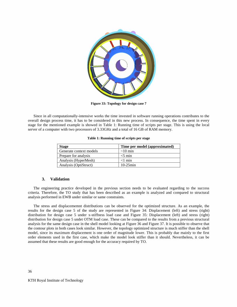
As an example, the first seven design cases of the DOE are run and the results are analyzed. Figure 32: Topology
for design case 5 and Figure 33: Topology for design case 7 show the resultant topology for two design cases. The
results for the other five cases appear in Example I of the appendix. Other examples with different constraints
appear in Example II and Example III.
Figure 32: Topology for design case 5
36
KTH Royal Institute of Technology
Figure 33: Topology for design case 7
Since in all computationally-intensive works the time invested in software running operations contributes to the
overall design process time, it has to be considered in this new process. In consequence, the time spent in every
stage for the mentioned example is showed in Table 1: Running time of scripts per stage. This is using the local
server of a computer with two processors of 3.33GHz and a total of 16 GB of RAM memory.
Table 1: Running time of scripts per stage
Stage Time per model (approximated)
Generate context models ~10 min
Prepare for analysis <5 min
Analysis (HyperMesh) <1 min
Analysis (OptiStruct) 10-25min
3. Validation
The engineering practice developed in the previous section needs to be evaluated regarding to the success
criteria. Therefore, the TO study that has been described as an example is analyzed and compared to structural
analysis performed in EWB under similar or same constraints.
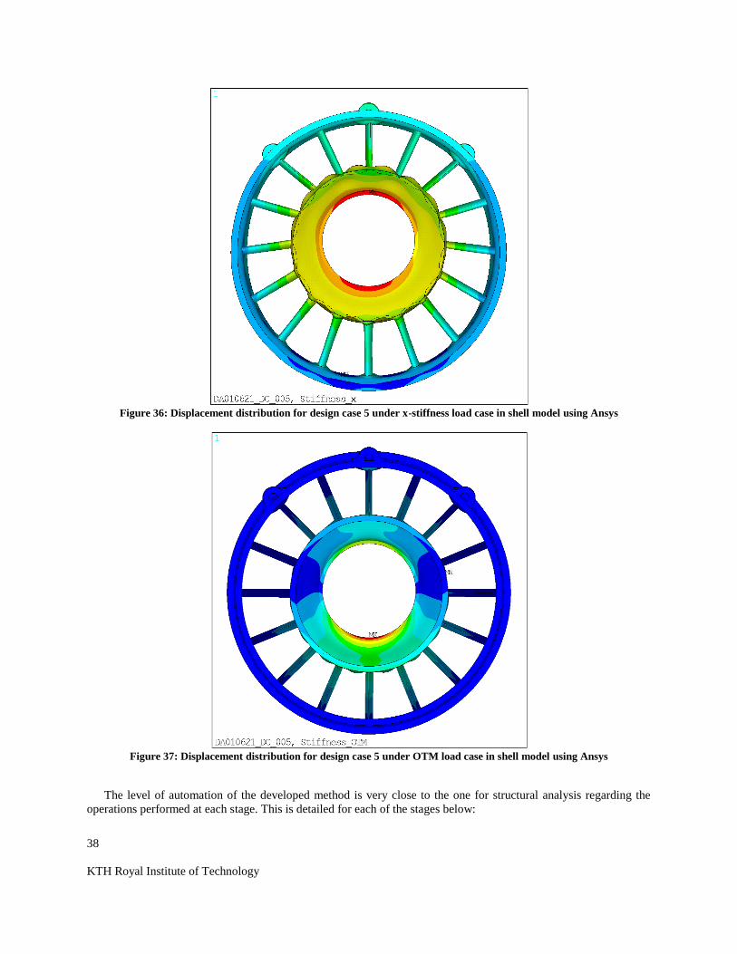
The stress and displacememnt distributions can be observed for the optimized structure. As an example, the
results for the design case 5 of the study are represented in Figure 34: Displacement (left) and stress (right)
distribution for design case 5 under x-stiffness load case and Figure 35: Displacement (left) and stress (right)
distribution for design case 5 undet OTM load case. These can be compared to the results from a previous structural
analysis for the same design case in the shell model looking at Figure 36 and Figure 37. It is possible to observe that
the contour plots in both cases look similar. However, the topology optimized structure is much stiffer than the shell
model, since its maximum displacement is one order of magnitude lower. This is probably due mainly to the first
order elements used in the first case, which make the model look stiffer than it should. Nevertheless, it can be
assumed that these results are good enough for the accuracy required by TO.

37
KTH Royal Institute of Technology
Figure 34: Displacement (left) and stress (right) distribution for design case 5 under x-stiffness load case in optimized
structure using HyperView
Figure 35: Displacement (left) and stress (right) distribution for design case 5 undet OTM load case in optimized
structure using HyperView
38
KTH Royal Institute of Technology
Figure 36: Displacement distribution for design case 5 under x-stiffness load case in shell model using Ansys
Figure 37: Displacement distribution for design case 5 under OTM load case in shell model using Ansys
The level of automation of the developed method is very close to the one for structural analysis regarding the
operations performed at each stage. This is detailed for each of the stages below:

39
KTH Royal Institute of Technology
Setup study
This stage requires work on the CAD model, creating the DOE of the study and scripting the input files for
the desired studies. These are the most manual intensive tasks in the process for the TO and the other older
studies.
Generate context model
Since the DOE and the CAD model can be set so either a shell model or a hybrid one can be selected
automatically, the level of automation of this stage is maintained. Moreover, it can be run in batch mode, as
in the case of the other discipline studies.
Prepare for analysis
Using the developed script for metadata execution and meshing, the FE model is generated as automatically
as before. It only requires selecting the settings previous to be run. Then, as when a structural study is
performed in Ansys, to obtain the final model for analysis, another script is used. This is because the settings
required in it are of different nature. Therefore, it is convenient to be able to modify this script without
modifying the other one. In addition, these scripts may also be run in batch mode, although this has not been
done within this thesis work.
Analysis
To perform the analysis, the scripts automatically generated in the previous stage is simply run in OptiStruct
and results are obtained. These scripts are selected in the solver and they are solved in queue. Consequently,
no additional human interventions are required.
Evaluate
Finally, as usually in EWB, once the results are obtained, they are examined by hand.
V. Discussion
The EWB process’ division into stages stages appears to be pretty convenient for the implementation of TO,
since the main steps of work corresponding to this method follow a very similar structure. The first three stages of
EWB are used to prepare the model, while the “Analysis” stage prepares the optimization. Then, the results are
interpreted in the “Eval ate” stage.
A good knowledge of the work performed in Siemens NX and HyperMesh for the existing structural analysis is a
good starting point for the implementation of TO, since same tools and type of scripts can be used. Nevertheless,
additional knowledge is required to be able to work with solids in the model. This is beacuse new metadata is
provided to the CAD model and many additional operations must be included in the scripts for HyperMesh. On the
other hand, as the structural analysis in EWB is always performed in Ansys, there is no reference to create the
required scripts. However, the reference guide in HyperMesh represents an important help for the task. Overall,
good knowledge of TCL scripting needs to be achieved, but basic understanding of the other coding languages is
enough for this work.
Automating the choice of hub type between the old sheet bodies and the new solid body is a good way of
implementing the MDO study. DOE can be set so some design cases are destinated to TO and others to structural
analysis without the need of repeating the stages where the FE models are created.
Another finding is that a deep understanding of the way to work in TO is fundamental for its implementation in
the EWB platform. The characteristics of the FE model generated previous to the optimization have a big influence
in the results and in the simulation time. Moreover, the selection of the parameters of the optimization as the
objective function, the optimization constraints and the manufacturing constraints have a great impact as well. Due
to time constraints, this thesis work only presents the development of the process for one combination of settings,
but a comparison between results coming from different combinations is recommended.
A great advantage of TO is that resulting optimized structures can be obtained with regard to several load cases
simultaneously. Some responses as the compliance even allow to give weight to the influence of each load case.
Thus, when the objective is to design a component that is exposed to many different load conditions, they should all
40
KTH Royal Institute of Technology
be applied in the study with the constraints that suit the best to each of them. At the current stage of development of
this implementation only linear static loads are applied. Nevertheless, there is potential for combining them with
other studies like heat transfer, which has not been done in this occasion because of time limitations.
After evaluating the results of stress and displacement from the TO, it is obvious that the accuracy of the method
is not very good from the point of view of the structural analysis. Nonetheless, the objective of this method is to
identify the locations in the design space that are more important for the structural integrity of the component. For
this, not very precise measurements of stress and displacement are required, the identification of the load paths is
sufficient. These values and the contour plots are helpful to confirm that there was no error during implementation.
The visualization of the element densities in ISO and contour plots is good for the understanding of the more
important areas of the structure. Experience and judgement are then used to decide design modifications. Exporting
the topology as a new geometry or FE model is pretty limited due to the very complex shapes obtained. This makes
difficult to work directly on it to create a new design. On the other hand, the information about mass received as
outcome of the study is only useful to give an approximated idea of the possible weight reduction. The mass is
actually calculated considering the fractions of the density corresponding to each element. Therefore, in a new
design, where the elements either have full density or they are removed, the mass would be different.
It is also relevant to mention that the time invested in simulations is relativey short for the example considered in
this thesis, which is very positive for the design process. However, as said before, changing settings in the process
might increment largely this time.
Finally, the level of automation of the solution can be considered acceptable. Nevertheless, due to lack of time,
the execution of all scripts in batch mode has not been implemented yet. Therefore, HyperMesh and OptiStruct need
to be open so as to run these scripts.
VI. Conclusions
A method for the implementation of TO in the MDO platform EWB has been presented. The automation
level of the method corresponds to other disciplines of the platform and the procedure has been developed starting
from the existing ones in order to avoid the need of many additional files and tools. The implementation of thermal,
producibility and aerodynamic aspects in TO has been regarded, although it has not been totally implemented. Some
requirements of producibility can be tackled through the use of manufacturing constraints available in OptiStruct.
Thermal boundary conditions may be applied through heat transfer load cases to add in the optimization, but this
thesis work did not study deeply this possibility. Furthermore, for components whose outer geometry has
requierements from aerodynamics, the choice of the design space needs of special attention. All parts of the structure
that should keep the external shape are assigned to a component designated as non-design space.
TO can improve the design process when combined with regular DOE approach in the EWB platform. While the
structural analysis contains a limited number of parameters regarding geometry variations, TO offers a great
flexibility in possible geometries. The optimized topologies can be used to derive conclusions about what parts of
the component are less important to carry the load of the structure. Hence, with the objective of reducing weight,
these parts may be removed or modified respecting constraints from other disciplines. Conjointly, completely new
design suggestions can be substracted as well. In any case, regular structural analysis should always be performed
for a new design to accurately prove that it fulfils the requirements.
VII. Further Work
As a consequence of the explorative work realized for this thesis and the time constraint, several suggestions
for further work are proposed in this section.

41
KTH Royal Institute of Technology
As mentioned formerly, the selection of settings to generate the FE model and to perform the optimization have a
considerable effect in the result. Therefore, to completely understand this effect, many studies with variation of
settings should be performed. In addition, in this thesis only seven design cases and two load cases have been
presented, since the objective was only to validate the implementation of the method. However, for a real use of the
method, many more design cases should be studied and all the load cases considered in the TRS should be applied.
The latter includes the heat transfer study, whose implementation should still be explored in detail. Moreover,
extending the design space to other componenets of the structure apart of the hub is also recommended to complete
the study.
On the other hand, since the execution of scripts in batch mode has not been totally implemented, this task
should be finished in the next steps after this thesis.
To conclude, for a more global validation of the scripts, the developed process should be applied to a different
component from the TRS. This would allow to add the necessary corrections and to create a procedure that works
for any study.
References
[1] Joaquim R.R.A. Martins, Andrew B. Lambe, "Multidisciplinary Design Optimization: Survey of
Architectures," AIAA Journal, 2013.
[2] Ding Yang, M. Turrin, S. Sariyildiz, Yimin Sun , "Sports building envelope optimization using multi-objective
multidisciplinary design optimization (M-MDO) techniques: Case of indoor sports building project in China,"
in IEEE Congress on Evolutionary Computation, 2015.
[3] Jeremy Agte, Olivier de Weck, Jaroslaw Sobieszczanski-Sobieski, Paul Arendsen, Alan Morris, Martin Spieck,
"MDO: assessment and direction for advancement—an opinion of one international group," in 2006 European-
U.S. Multidisciplinary Optimization (MDO) Colloquium in Goettingen, 2009.
[4] Melissa Gardenghi, Margaret M. Wiecek, "Efficiency for multiobjective multidisciplinary optimization
problems with quasiseparable subproblems," Springer Science+Business Media, LLC, 2011.
[5] G. L. Rocca, "Knowledge based engineering: Between AI and CAD. Review of a language based technology to
support engineering design.," Advanced Engineering Informatics Journal, vol. Vol. 26, pp. 159-179, 2012.
[6] S. Quintana-Amate, P. Bermell-Garcia, A. Tiwari, C.J. Turner, "A new knowledge sourcing framework for
knowledge-based engineering: An aerospace industry case study," Computers & Industrial Engineering, vol.
104, pp. 35-50, 2016.
[7] Vibhor Trehan, Craig Chapman, Pathmeswaran Raju, "Informal and formal modeling of engineering processes
for design automation using knowledge based engineering," Zhejiang University-SCIENCE A (Applied Physics
& Engineering), vol. 16(9), pp. 706-723, 2015.
[8] C. E. Levandowski, "PhD thesis: Platform Lifecycle Support using Set-Based Concurrent Engineering,"
Chalmers University of Technology, Gothenburg, Sweden, 2014.
[9] James M. Morgan, Jeffrey K. Liker, The Toyota Product Development System, New York, USA: Productivity
Press, 2006.
[10] Christoffer Levandowski, Marcel T Michaelis, Hans Johannesson, "Set-based development using an integrated
product and manufacturing system platform.," Concurrent Engineering: Research and Applications, vol. 22(3),
pp. 234-252, 2014.
[11] Nestor V. Queipo, Raphael T. Haftka, Wei Shyy, Tushar Goel, Rajkumar Vaidyanathan, P. Kevin Tucker,
"Surrogate-based analysis and optimization," Progress in Aerospace Sciences, vol. 41, pp. 1-29, 2005.
[12] J. Paulo, Design of Experiments in Production Engineering. Management and Industrial Engineering, vol. 1,
Springer, 2016, pp. 3-4.
[13] Veli-Matti Tapani Taavitsainen, "Experimental Optimization and Response Surfaces," in Chemometrics in
Practical Applications, InTech, 2012, pp. 91-138.

42
KTH Royal Institute of Technology
[14] Gilbert Chahine, Pauline Smith, Radovan Kovacevic, "Application of Topology Optimization in Modern
Additive Manufacturing," in Solid Freeform fabrication Symposium, Austin, Texas, 2010.
[15] A. Freeman, "Topology Optimisation and Additive Manufacturing of Formula Student Uprights - Final
Report," GKN Aerospace & University of Bath, 2014.
[16] Razvan Cazacu, Lucian Grama, "Overview of Structural Topology Optimization Methods for Plane and Solid
Structures," Annals of the Oradea University: Fascicle Management and Technological Engineering, 2014.
[17] K. James, "Aerostructural Shape and Topology Optimization of Aircraft Wings," University of Toronto, 2012.
[18] "HyperWorks Online Help," Altair, [Online]. Available: http://www.altairhyperworks.com. [Accessed 2017].
[19] "GKN at a Glance," GKN, [Online]. Available: http://www.gkn.com/en/about-gkn/. [Accessed 12 06 2017].
[20] "About GKN Aerospace," GKN, [Online]. Available: http://www.gkn.com/en/our-divisions/gkn-
aerospace/about-gkn-aerospace/. [Accessed 12 06 2017].
[21] "GKN in Europe," GKN, [Online]. Available: http://www.gkn.com/en/about-gkn/locations/gkn-in-europe/.
[Accessed 12 06 2017].
[22] "Om GKN Aerospace Sweden," GKN, [Online]. Available:
http://www.gkngroup.com/GKNSweden/aerospace/om-gkn-aerospace-sweden/Pages/default.aspx. [Accessed
12 06 2017].
[23] "About NX Software," Siemens PLM Software, [Online]. Available:
https://www.plm.automation.siemens.com/en_us/products/nx/about-nx-software.shtml. [Accessed 12 06 2017].
[24] "Programming Tools," Siemens PLM Software, [Online]. Available:
https://docs.plm.automation.siemens.com/tdoc/nx/10/nx_api/#uid:index. [Accessed 12 06 2017].
[25] The Jet Engine, Rolls-Royce, 2005.
[26] Amaresh Chakrabarti, "A course for teaching design research methodology. Artificial Intelligence for
Engineering Design," Artificial Intelligence for Engineering Design, Analysis and Manufacturing, vol. 24, pp.
pp 317-334, 2010.
[27] Pierre Duysinx, Michael Bruyneel, "Recent Progress in Preliminary Design of Mechanical Component with
Topology Optimization," University of Liège, Mechanical Institute, Liège, Belgium.
[28] M. Johansson, "Topology Optimization using OptiStruct," GKN Aerospace Sweden AB, Trollhättan, Sweden,
2016.
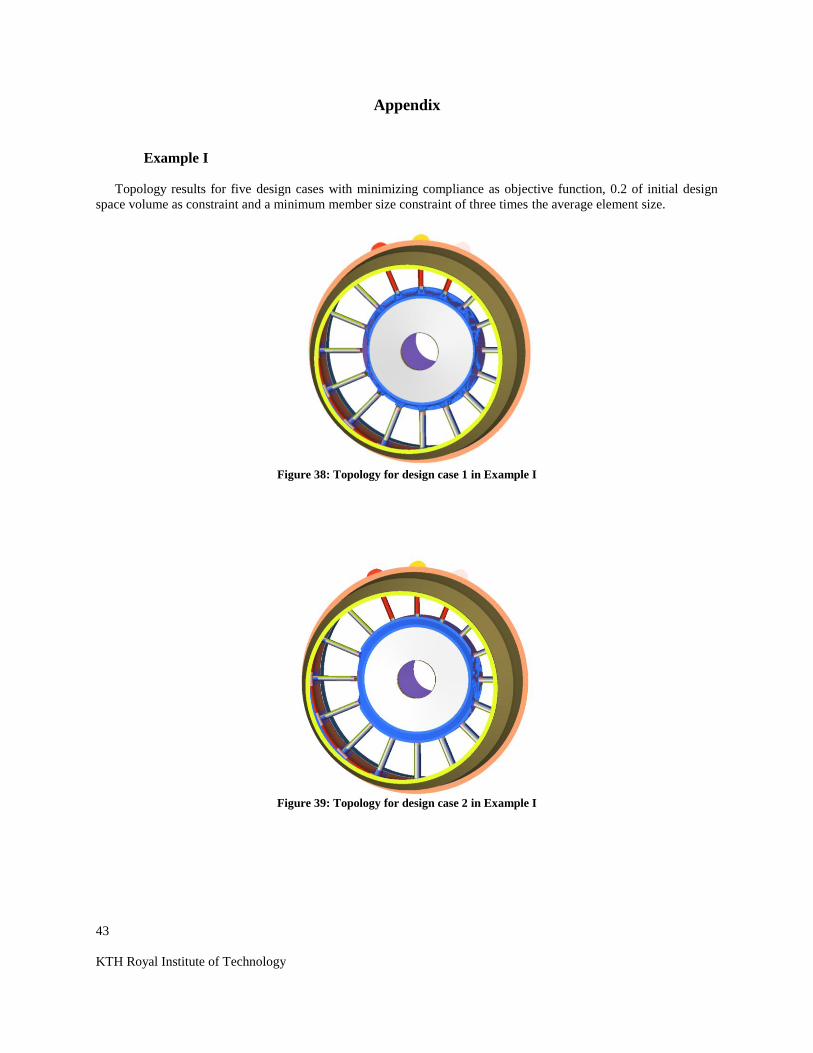
43
KTH Royal Institute of Technology
Appendix
Example I
Topology results for five design cases with minimizing compliance as objective function, 0.2 of initial design
space volume as constraint and a minimum member size constraint of three times the average element size.
Figure 38: Topology for design case 1 in Example I
Figure 39: Topology for design case 2 in Example I

44
KTH Royal Institute of Technology
Figure 40: Topology for design case 3 in Example I
Figure 41: Topology for design case 4 in Example I
Figure 42: Topology for design case 6 in Example I

45
KTH Royal Institute of Technology
Example II
Topology results for seven design cases with minimizing compliance as objective function, 0.1 of initial design
space volume as constraint and a minimum member size constraint of three times the average element size.
Figure 43: Topology for design case 1 in Example II
Figure 44: Topology for design case 2 in Example II
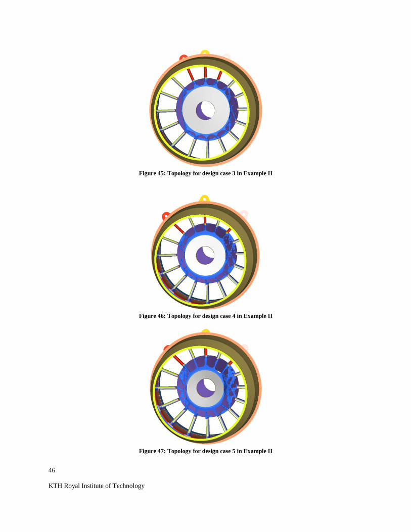
46
KTH Royal Institute of Technology
Figure 45: Topology for design case 3 in Example II
Figure 46: Topology for design case 4 in Example II
Figure 47: Topology for design case 5 in Example II
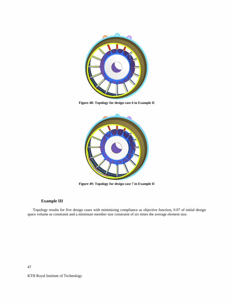
47
KTH Royal Institute of Technology
Figure 48: Topology for design case 6 in Example II
Figure 49: Topology for design case 7 in Example II
Example III
Topology results for five design cases with minimizing compliance as objective function, 0.07 of initial design
space volume as constraint and a minimum member size constraint of six times the average element size.
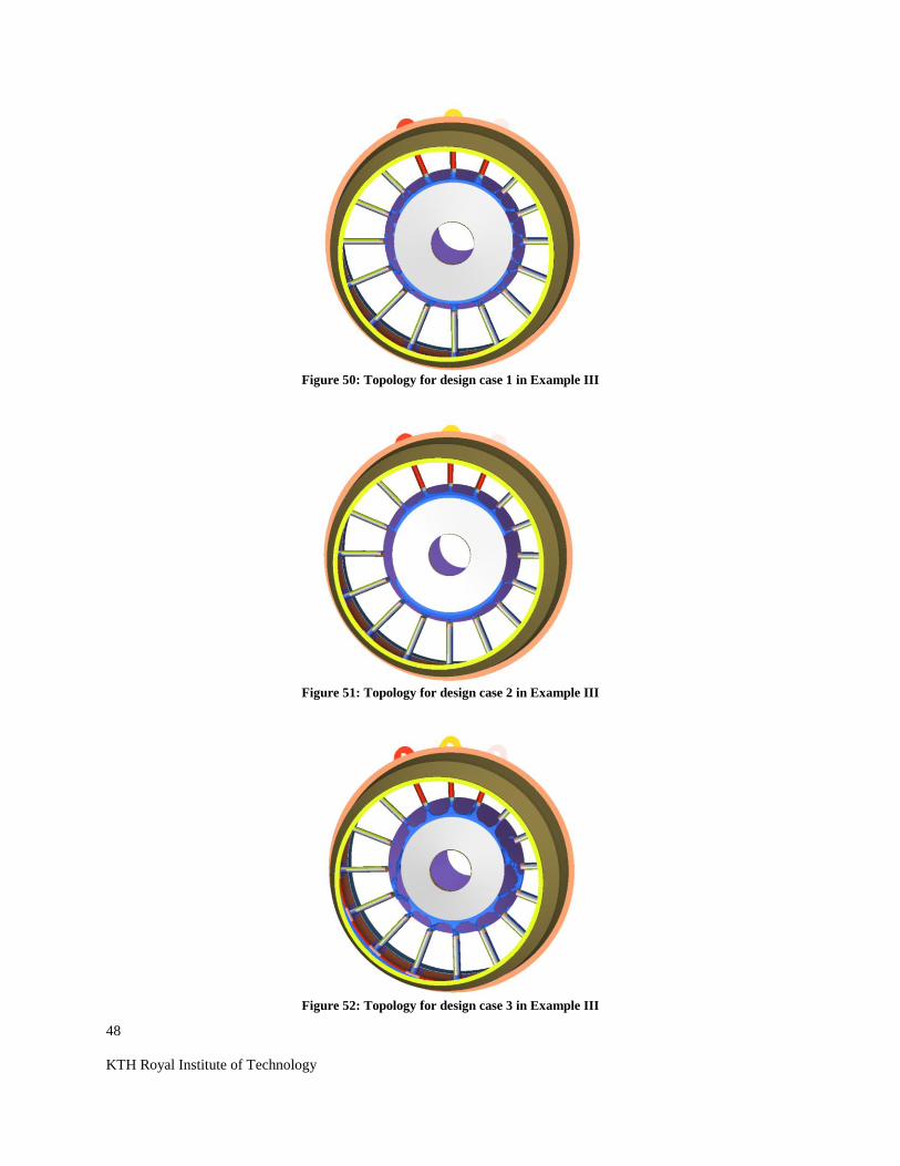
48
KTH Royal Institute of Technology
Figure 50: Topology for design case 1 in Example III
Figure 51: Topology for design case 2 in Example III
Figure 52: Topology for design case 3 in Example III

49
KTH Royal Institute of Technology
Figure 53: Topology for design case 4 in Example III
Figure 54: Topology for design case 5 in Example III
Figure 55: Topology for design case 6 in Example III

50
KTH Royal Institute of Technology
Figure 56: Topology for design case 7 in Example III
List of Figures
Figure 1: SBCE method for an aircraft engine component development ...................................................................... 9 Figure 2: DOE structure [12] ....................................................................................................................................... 10 Figure 3: Before and after TO with SIMP [18] ............................................................................................................ 11 Fig re 4: EWB’s MDO approach ................................................................................................................................ 13 Figure 5: EWB study work flow .................................................................................................................................. 13 Figure 6: Commercial aircraft engine with the TRS highlighted [25] ......................................................................... 14 Figure 7: TRS of a commercial aircraft engine [25] .................................................................................................... 15 Figure 8: Stages in Design Research Methodology [26] ............................................................................................. 16 Figure 9: CAD assembly of TRS ................................................................................................................................. 18 Figure 10: Connections between DOE Excel file and CAD model ............................................................................. 19 Figure 11: Different design cases obtained automatically ........................................................................................... 20 Fig re 12: Model bro ser in Hypermesh after “Generate context models” stage ....................................................... 20 Figure 13: Wireframe of model in Hypermesh after “Generate context models” stage .............................................. 21 Fig re 14: Process in “Generate context models” stage .............................................................................................. 21 Fig re 15: Process in “Generate context models” stage hen r n in batch mode ....................................................... 22 Fig re 16: Model bro ser in Hypermesh after “Prepare for analysis” stage ............................................................... 23 Figure 17: Property collector information in HyperMesh ........................................................................................... 23 Figure 18: FE model in Hypermesh after “Prepare for analysis” stage ....................................................................... 24 Fig re 19: Process in “Prepare for analysis” stage ...................................................................................................... 24 Fig re 20: Process in “Prepare for analysis” stage hen r n in batch mode ............................................................... 25 Figure 21: Structural analysis results obtained in Ansys for a number of design cases ............................................... 25 Figure 22: Bad connectivity between mesh in two adyacent components ................................................................... 26 Figure 23: TO result without manufacturing constraints (left) and with minimum member size control (right) ........ 28 Figure 24: ISO plot with element density thresholds 0.2 (up and left), and combination of ISO and contour plots with
element density thresholds 0.2 (up and right), 0.5 (down and left) and 0.8 (down and right) ..................................... 29 Figure 25: CAD assembly of TRS with solid hub ....................................................................................................... 30 Figure 26: Section of the two hub alternatives for the TRS model .............................................................................. 31 Figure 27: Property collector information for the solid hub component in HyperMesh .............................................. 32 Fig re 28: FE model in Hypermesh after “Prepare for analysis” stage for TO ........................................................... 32 Figure 29: Model browser in Hypermesh after “Analysis” stage for TO .................................................................... 34 Fig re 30: FE model in Hypermesh after “Analysis” stage for TO ............................................................................. 34

51
KTH Royal Institute of Technology
Fig re 31: Process in “Analysis” stage for TO ............................................................................................................ 35 Figure 32: Topology for design case 5 ........................................................................................................................ 35 Figure 33: Topology for design case 7 ........................................................................................................................ 36 Figure 34: Displacement (left) and stress (right) distribution for design case 5 under x-stiffness load case in
optimized structure using HyperView ......................................................................................................................... 37 Figure 35: Displacement (left) and stress (right) distribution for design case 5 undet OTM load case in optimized
structure using HyperView .......................................................................................................................................... 37 Figure 36: Displacement distribution for design case 5 under x-stiffness load case in shell model using Ansys ....... 38 Figure 37: Displacement distribution for design case 5 under OTM load case in shell model using Ansys ............... 38 Figure 38: Topology for design case 1 in Example I ................................................................................................... 43 Figure 39: Topology for design case 2 in Example I ................................................................................................... 43 Figure 40: Topology for design case 3 in Example I ................................................................................................... 44 Figure 41: Topology for design case 4 in Example I ................................................................................................... 44 Figure 42: Topology for design case 6 in Example I ................................................................................................... 44 Figure 43: Topology for design case 1 in Example II.................................................................................................. 45 Figure 44: Topology for design case 2 in Example II.................................................................................................. 45 Figure 45: Topology for design case 3 in Example II.................................................................................................. 46 Figure 46: Topology for design case 4 in Example II.................................................................................................. 46 Figure 47: Topology for design case 5 in Example II.................................................................................................. 46 Figure 48: Topology for design case 6 in Example II.................................................................................................. 47 Figure 49: Topology for design case 7 in Example II.................................................................................................. 47 Figure 50: Topology for design case 1 in Example III ................................................................................................ 48 Figure 51: Topology for design case 2 in Example III ................................................................................................ 48 Figure 52: Topology for design case 3 in Example III ................................................................................................ 48 Figure 53: Topology for design case 4 in Example III ................................................................................................ 49 Figure 54: Topology for design case 5 in Example III ................................................................................................ 49 Figure 55: Topology for design case 6 in Example III ................................................................................................ 49 Figure 56: Topology for design case 7 in Example III ................................................................................................ 50

TRITA AVE 2017:62
ISSN 1651-7660
www.kth.se