Topology optimization analysis based on the direct

ORIGINAL RESEARCH

Topology optimization analysis based on the direct couplingof the boundary element method and the level set method

Paulo Cezar Vitorio Jr.1 • Edson Denner Leonel1

Received: 20 March 2017 / Accepted: 9 October 2017 / Published online: 24 October 2017

� The Author(s) 2017. This article is an open access publication

Abstract The structural design must ensure suit-

able working conditions by attending for safe and eco-

nomic criteria. However, the optimal solution is not easily

available, because these conditions depend on the bodies’

dimensions, materials strength and structural system con-

figuration. In this regard, topology optimization aims for

achieving the optimal structural geometry, i.e. the shape

that leads to the minimum requirement of material,

respecting constraints related to the stress state at each

material point. The present study applies an evolutionary

approach for determining the optimal geometry of 2D

structures using the coupling of the boundary element

method (BEM) and the level set method (LSM). The pro-

posed algorithm consists of mechanical modelling, topol-

ogy optimization approach and structural reconstruction.

The mechanical model is composed of singular and hyper-

singular BEM algebraic equations. The topology opti-

mization is performed through the LSM. Internal and

external geometries are evolved by the LS function eval-

uated at its zero level. The reconstruction process concerns

the remeshing. Because the structural boundary moves at

each iteration, the body’s geometry change and, conse-

quently, a new mesh has to be defined. The proposed

algorithm, which is based on the direct coupling of such

approaches, introduces internal cavities automatically

during the optimization process, according to the intensity

of Von Mises stress. The developed optimization model

was applied in two benchmarks available in the literature.

Good agreement was observed among the results, which

demonstrates its efficiency and accuracy.

Keywords Boundary element method � Topology

optimization � Level set function

Introduction

The structural engineer aims at attaching two targets that

are normally, opposite: safety and economy. In the most

part of structural designs, the optimal solution, i.e. the

solution that couples perfectly such targets, is not easily

available because it depends on the material characteristic

strengths, structural dimensions and structural system

adopted. To solve consistently such engineering challenge

problem, special theories/techniques have recently

emerged (Bendsøe and Kikuchi 1988; Rozvany et al. 1992;

Maute and Ramm 1995). Among them, it is worth men-

tioning the topology optimization. This domain aims for

designing the geometry of structural components with

proper safety level accounting for the minimum require-

ment of material. Thus, this type of optimization achieves

the optimal structural geometry, the shape that leads to the

minimum requirement of material, respecting constraints

related to the stress state at each material point.

The mechanical modelling of structures may be

accomplished through analytical approaches, which are

normally based on the theory of elasticity. However, the

solutions provided by this theory are limited to simplified

geometries, boundary conditions and material constitutive

relations. Thus, to enable a general mechanical modelling

numerical methods are required. The present study utilized

the boundary element method (BEM), which is recognized

& Edson Denner Leonel

[email protected]

1 School of Engineering of Sao Carlos, Department of

Structural Engineering, University of Sao Paulo,

Av. Trabalhador Sao Carlense, 400, Sao Carlos,

SP 13566-590, Brazil

123

Int J Adv Struct Eng (2017) 9:397–407

https://doi.org/10.1007/s40091-017-0175-8

http://crossmark.crossref.org/dialog/?doi=10.1007/s40091-017-0175-8&domain=pdf

http://crossmark.crossref.org/dialog/?doi=10.1007/s40091-017-0175-8&domain=pdf

https://doi.org/10.1007/s40091-017-0175-8

as a robust and efficient numerical technique. The BEM is

capable for handling accurately several types of mechani-

cal problems. Due to its mesh dimension reduction and

accuracy in determining stress concentration fields, the

BEM becomes well adapted for solving topology opti-

mization problems.

The topology optimization was initially proposed in the

end of 1980s by Bendsøe (1989), which analysed the

material distribution into a fixed domain. The optimal

structural geometry was achieved through the definition of

a material density, which may vary from a void until the

full presence of material. An intermediate material density

may be also assumed. The bubble method was introduced

by Eschenauer et al. (1994), which is based on the insertion

of cavities in the structure and the subsequent use of the

shape optimization method for determining the optimal

structural size and shape. The simpler evolutionary struc-

tural optimization (ESO) method, presented by Xie and

Steven (1993), removes material progressively from low

stress regions based on a given acceptation/rejection cri-

teria. This technique was widely applied with finite ele-

ment models due to the domain mesh required in such

models.

Topology optimization analyses in two- and three-di-

mensional structures using the BEM are presented in

Cervera and Trevelyan (2005a, b). In their ESO approach,

the moving structural geometry was represented explicitly

through the NURBS, in which the spline control points is

moved according to the response of local stress values. The

boundary element-based topological derivatives concept

was used for the first time by Marczak (2007), for the

topology optimization of thermally conducting solids. The

proposed formulation was based on introducing an iterative

material removal procedure in a BEM framework. Topol-

ogy optimization in 2D elastic structures through the BEM

is presented in Neches and Cisilino (2008). Linear

boundary elements were adopted and small cavities are

inserted around internal points with the lowest values of the

topological derivative. The topology optimization in a 3D

BEM elastostatic framework taking into account the

topological shape sensitivity method for the direct calcu-

lation of topological derivatives from stress fields is

introduced in Bertsch et al. (2010). The shape derivatives

were combined with topological derivatives by Allaire and

Jouve (2008), to propose a level set-based optimization

method capable for automatic hole insertion.

An efficient approach in the topology optimization

domain consists of the level set method (LSM). This

method was proposed, initially, to model the movement of

curves (Osher and Sethian 1988; Sethian 1999). When the

LSM is applied in the structural context, the mentioned

curves represent the structural boundary and its movement/

evolution characterizes the new/optimized structural

geometry. The LSM is based on the solution of Hamilton–

Jacobi differential equations. The LSM represents the

structural geometry as well as its evolution through the

zero level of an important function denominated level set

(LS) (Osher and Sethian 1988; Sethian 1999; Shichi et al.

2012; Yamada et al. 2013; Osher and Fedkiw 2003).

In the present study, the topology optimization analysis

is developed accounting for the direct coupling of BEM–

LSM. The proposed algorithm consists of three parts:

mechanical modelling, topology optimization procedure

and structural reconstruction. The mechanical modelling is

accomplished through the BEM algebraic equations, in

which singular and hyper-singular integral representations

may be applied.

The singular integral equation represents accurately the

mechanical material behaviour in the most part of elasto-

static problems. However, the application of this integral

equation for source points nearly positioned may lead to

the singularities on the final system of algebraic equations

due to the singular nature of the fundamental solutions.

Such singularities are avoided using the hyper-singular

integral equation in addition to the first mentioned integral

equation. During the topology evolution process, complex

geometries may appear leading to nearly positioned source

points. Thus, in this study, the singular and hyper-singular

integral equations are utilized into the discretization in

order to provide numerical stability, which is one contri-

bution of this study.

The topology optimization procedure is performed using

the LSM approach. The structural geometry is described by

the LS function evaluated at its zero level. The velocities of

moving boundaries are determined according to the Von

Mises stress intensity at each boundary node. The coupling

between the LSM and the Von Mises stresses provided by

BEM is direct. Thus, velocity extension scheme is not

required, which is another contribution of this study.

Finally, the reconstruction process concerns the

remeshing procedure. Because the boundary moves at each

iteration, the structural geometry change and a new mesh

has to be constructed. The new mesh is proposed

accounting for the source points position. Then, singular

and hyper-singular integral equations are proper applied.

During the topology optimization process, internal cavities

may be introduced automatically, in order to accelerate the

numerical convergence. The internal cavities are punctu-

ally included where the Von Mises stress is lower than an

established threshold. The boundaries of such cavities may

grow or collapse according to the Von Mises stress. This is

one advantage of LSM, in which material may be removed

or include in automatic and in consistent form.

Two applications are presented in the present study to

illustrate the relevance of the presented framework. The

398 Int J Adv Struct Eng (2017) 9:397–407

123

results obtained by the presented scheme are in good

agreement with the responses provided by the literature.

The boundary element method

The BEM has been widely utilized in engineering fields

such as contact mechanics and fracture mechanics due to

its high accuracy and robustness in modelling strong stress

concentration. In addition to this inherent ability of the

BEM, its mesh dimension reduction makes this numerical

method well adapted to solve topology optimization

problems. The integral equations required by the BEM are

obtained from the equilibrium equation. Considering a 2D

homogeneous elastic domain, X, with boundary, C, the

equilibrium equation, written in terms of displacements, is

given by

ui;jj þ1

1 � 2tuj;ji þ

bi

l¼ 0 ð1Þ

in which l is the shear modulus, t is the Poisson’s ratio, uiare the components of the displacement field, and bi are the

body forces.

Afterwards, the Betti’s theorem is utilized and the sin-

gular integral representation, written in terms of displace-

ments, is obtained (without body forces) as follows:

cijðs; f ÞujðsÞ þZ

C

P�ijðs; f Þujðf ÞdC ¼

Z

C

U�ijðs; f Þpj fð ÞdC

ð2Þ

in which pj and uj are tractions and displacements at the

field points f , respectively, the free term cij is equal to dij�2

for smooth boundaries and P�ij and U�

ij are the fundamental

solutions for tractions and displacements written for the

source point s (Brebbia and Dominguez 1992; Hong and

Chen 1988).

The Eq. (2) has to be differentiated with respect to the

directions x, y, in order to obtain an integral equation

written in terms of strains. Then, the use of the generalized

Hooke’s law leads to the integral representation of stresses

for a boundary source point. Finally, the Cauchy formula

has to be applied for obtaining the hyper-singular integral

equation, which is written in terms of tractions as follows:

1

2pjðsÞ þ gi

Z

C

S�ijkðs; f Þukðf ÞdC ¼ gi

Z

C

D�ijkðs; f Þpkðf ÞdC

ð3Þ

in which S�ijk and D�ijk contain the new kernels computed

from P�ij and U�

ij, respectively, (Brebbia and Dominguez

1992; Hong and Chen 1988) and gk is the outward normal

vector.

To assemble the system of BEM equations, as usual,

Eq. (2) or Eq. (3) are transformed into algebraic relations

by discretizing the structural boundary into elements over

which displacements and tractions are approximated. In the

present study, only linear discontinuous boundary elements

are applied. The regular integrals were calculated using

Gauss–Legendre quadrature whereas the singularity sub-

traction technique was applied in the integration over sin-

gular boundary elements. The discretization of external

boundary into boundary elements leads to the following

system of algebraic equations:

Hu ¼ Gp ð4Þ

where u and p are vectors that contain displacements and

tractions at the boundary source points, respectively. The

matrix H contains the terms evaluated numerically from

the kernels P�ij or S�ijk whereas G is composed by the terms

calculated from the kernels U�ij or D�

ijk.

After determining the displacement and traction fields at

the boundary, internal values for displacements, stresses

and strains are achieved. Internal displacements are deter-

mined through the integral equation Eq. (2) with the source

point positioned at the domain. In such case, the free term

cij becomes dij. On the other hand, the stress field at

internal nodes is obtained through the integral representa-

tion of stresses (Brebbia and Dominguez 1992; Hong and

Chen 1988).

The level set method

The LSM is a robust technique for simulating and for

determining the movement of curves in different physical

scenarios. Such method represents a particular curve (or

surface) C as well as its movement/evolution along time as

the zero level of a major function U, which is denominated

Fig. 1 Level Set Function. Circle evolution due to a conical surface

Int J Adv Struct Eng (2017) 9:397–407 399

123

level set (LS) function. Figure 1 illustrates a classical

example of one LS function. This figure illustrates the

movement/evolution of a circle, which LS function is

conical. The LS equation and its evolutions, for general

cases, are represented in the following form:

Ut þ V!�rU ¼ 0 ð5Þ

in which Ut is the partial time derivative, V!

is the velocity

field at the grid points and rU is the gradient of the Ufunction, which represents the gradient of the partial

derivatives according to x and y directions.

By solving Eq. (5), through the finite differences for

instance, the values of U are determined for all points that

belong to the domain analysed. Therefore, based on the Uvalues, the new structural boundaries are achieved. The

LSM is capable of eliminating complexities of movement

of curves such as singularities, weak solutions, shocks

formation, non-stable conditions of entropy and topology

changes that involve interfaces. In the context of numerical

analysis, the LSM utilizes natural and accurate computa-

tional procedures. The method represents accurately cor-

ners and geometry ends as well as topology discontinuities.

Topology optimization by the direct couplingof BEM–LSM

As previously mentioned, the topology optimization anal-

ysis is developed based on the direct coupling of BEM–

LSM. The developed numerical procedure consists of three

parts: mechanical modelling, topology optimization pro-

cedure and structure reconstruction.

The mechanical modelling is accomplished by the BEM.

The BEM requires the structural boundaries discretization

by nodes and elements in order to determine stresses and

displacements at the structural boundaries into the struc-

tural domain. The structural boundaries geometries are

described through the LS function evaluated at its zero

level. Then, the curve delimited by the LS function at its

zero level is discretized into linear discontinuous boundary

elements.

When the source points are nearly positioned into the

BEM mesh, singularities at the final system of algebraic

equations may appear. Such singularities occur due to the

singular nature of the fundamental solutions required by

the BEM. Thus, to avoid these types of singularities, sin-

gular and hyper-singular integral equations are utilized in

the presented model. These integral equations are alter-

nately utilized along the boundary mesh when the distance

between a given source point and its closest source point is

lower than 10% of the boundary element length that con-

tains the given source point. It is worth mentioning that

nearly positioned source points often appear in this prob-

lem, because the topology evolution procedure leads to the

intermediate complex geometries before the convergence.

Thus, the proposed scheme leads to the stable and accurate

BEM responses.

An Eulerian mesh is required for solving the topology

optimization problem, which is defined by a rectangular

grid, Fig. 2. This mesh is responsible for approximating the

LS function values along the entire design domain.

Therefore, nil values for the LS function are observed at

the structural boundaries. The LS values at the Eulerian

grid points are evolved along the topology optimization

procedure, similarly as presented in Yamasaki et al. (2012).

The velocity criterion for evolving the structural bound-

aries is presented below. Then, the structural geometry is

immersed into the Eulerian grid and the structural geo-

metrical coordinates, which introduce nil LS values,

become a part of such mesh. It is worth mentioning that the

structural boundaries do not coincide, necessarily, with the

Eulerian grid points because the structure is immersed into

this grid. Thus, for each grid point, the LS function is

determined. Initially, such function is defined as the ori-

entated distance between the grid points and the structural

boundary.

The Eulerian grid points positioned inside the boundary

are represented by negative values of U. On the other hand,

the positive values of U indicate points positioned outside

the boundary. Finally, nil value of U defines the zero LS

and, consequently, the structural boundary. Thus, the sign

for U function is written as presented in Eq. (6).

Fig. 2 Eulerian mesh and structural immersion


123

U[ 0 outer design domain points

U ¼ 0 boundary design points

U\0 inner design domain points

ð6Þ

In this study, Eq. (5) is solved using the upwind differ-

ences method (Sethian 1999). This method calculates the

partial derivatives of the LS function in relation to x and y

directions. The time interval required by the method is

considered as fictitious and the number of evolutions carried

out at each iteration must be defined. BecauseUt�1 andU are

known at each Eulerian grid point, a velocity functionV!

must

be defined to enable the LS evolution process. The velocity

function depends of the Von Mises stress values at each

Eulerian grid point. Such dependence is consistent because

the topology optimization is applied in solid mechanics

problems (in potential problems the flux could derive the

moving boundaries velocity, for instance). Thus, the objec-

tive of the topology optimization performed in this study is

the determination of the structural geometry in which all

structural material points have the same Von Mises stress

values. As a result, the optimized structural material has the

same stress state, which defines the fully stressed design

approach and the maximum use of the mechanical material

capacity. The Von Mises stress is presented in Eq. (7), which

has to be evaluated for each Eulerian grid point.

rvm ¼ 1ffiffiffi2

pffiffiffiffiffiffiffiffiffiffiffiffiffiffiffiffiffiffiffiffiffiffiffiffiffiffiffiffiffiffiffiffiffiffiffiffiffiffiffiffiffiffiffiffiffiffiffiffiffiffiffiffiffiffiffiffiffiffiffiffiffiffiffiffiffiffiffiffiffiffiffiffiffiffiðr1 � r2Þ2 þ ðr2 � r3Þ2 þ ðr3 � r1Þ2

qð7Þ

in which r1, r2 and r3 indicate the principal stresses.

The Von Mises stress is evaluated by the BEM at each

grid point. Therefore, inefficient structural material is pro-

gressively removed as well as required structural material is

added where necessary. Such regions are determined natu-

rally through the evolution of the LS function. To define the

velocity function for moving boundaries according to the

intensity of the Von Mises stress, stress intervals are

required. Thus, a heuristic approach is utilized for govern-

ing the moving boundaries velocity. Such intervals are

expressed as a function of rvm, RR, ry and rmax, which are

the Von Mises stress, the removal rate, yield stress and

maximum Von Mises stress, respectively. The velocity

criteria adopted in this study, Vn, and recommended by

Ullah et al. (2014), are presented in Eq. (8).

rvm 2 0; rt1½ �:rt1 ¼ 0:5RRrmax Vn ¼ �1

rvm 2 rt1; rt2½ �:rt2 ¼ 0:9RRrmax Vn 2 �1; 0½ �rvm 2 rt2; rt3½ �:rt3 ¼ 0:95minðrmax; ryÞ Vn ¼ 0

rvm 2 rt3; rt4½ �:rt4 ¼ minðrmax; ryÞ Vn 2 0; 1½ �rvm 2 rt4;1½ �: Vn ¼ 1

ð8Þ

The negative velocities indicate point movement in the

inner boundary direction. Thus, negative velocities are

related to the removing material condition. Similarly, the

point movement in the outer direction is related to positive

velocities. In such condition, structural material is added.

Nil velocity indicates non-movement for the points. The

criterion presented in Eq. (8) is illustrated in Fig. 3.

Therefore, the moving boundaries are governed by the

criterion described in Eq. (8). To improve the convergence

rate, internal cavities are automatically introduced during

the topology evolution. Such cavities are included in points

where the Von Mises stress reaches a threshold value. The

analyst defines the threshold value and just one cavity per

iteration is allowed. In the present study, the cavity inclu-

sion obeys the criterion defined in Eq. (9).

rvm\RR rmax ð9Þ

The cavity radius is equal to the minimum value

between Dx and Dy, which are illustrated in Fig. 2. The

cavity inclusion allows for faster convergence as the

material is removed in regions with very low stress state.

Then, the removing procedure is improved with the cavities

inclusion. The cavity inclusion procedure is inspired in the

classical ESO approaches. However, the scheme proposed

in this study enables for adding material condition, when

the material is removed in a non-proper region. This is an

improvement over the classical ESO approaches in which

hard-kill conditions are often utilized.

The direct coupling BEM–LSM requires an update mesh

procedure. Because of the structural boundary change at

each LSM iteration, the boundary mesh considered in the

previous iteration must be eliminated and a new boundary

mesh must be constructed at the new zero LS. Thus, a

complex remeshing procedure must be performed. The

developed remeshing algorithm is capable of recognizing

the amount of curves present in the structure (outer and

inner boundaries) and to achieve the zero LS as the final

Fig. 3 Variation of Von Mises stress versus velocity


123

boundary. Such mapping procedure accounts for the LS

values at each Eulerian grid point. Then, the zero LS is

discretized into nodes and linear discontinuous boundary

elements for further analysis of the BEM. This process is

repeated until the desired optimal geometry be reached. To

assist computational implementation by the reader, a

flowchart is introduced and presented in Fig. 4.

Examples

The direct BEM–LSM formulation presented in this study

is applied in the topology optimization analysis of two

structures. One tensile case and one bending case were

chosen. In both analyses, the results obtained agree with

the responses available in the literature.

Two bar truss problem

The first application of the presented direct BEM–LSM

formulation concerns the topology optimization of the

plane structure illustrated in Fig. 5. This structure is

Fig. 4 BEM–LSM scheme for 2D topology optimization

Fig. 5 Structure analysed. Dimensions in metre

Fig. 6 Geometry evolution process

Fig. 7 Structural area evolution during the numerical procedure


123

clamped along two regions at its left end and is subjected to

a pointed load positioned at the middle of its right end. The

material properties utilized for this analysis are the fol-

lowing: Young’s modulus E ¼ 210 GPa, Poisson ratio t ¼0; 3 and material yield stress ry ¼ 280 MPa.

The reduction factor utilized in this analysis is equal to

RR ¼ 0:10. Moreover, 10 evolutions for each time step

into the upwind difference method were applied. The fic-

titious time used is Dt ¼ 0:003. The Eulerian mesh adopted

for solving the problem is composed of a grid with 67 �

45 points. Thus, 3015 points compose the grid. The values

of Dx and Dy are equal to Dx ¼ Dy ¼ 0:10 m.

In this analysis, one aims to obtain the structural

geometry that, after optimized, contains 40% of the initial

structural volume. Thus, the application of the direct

BEM–LSM formulation leads to the geometry evolution

presented in Fig. 6, which resembles a two-bar truss

structure. The internal cavities were included during the

evolution process and it accelerated the convergence pro-

cess. Moreover, the symmetric aspects were kept and the

Fig. 8 LS functions and its evolutions during the optimization process


123

result obtained agrees with classical references (Yamada

et al. 2013; Ullah et al. 2014).

The evolutional behaviour of the structural area values

during the iterative process is illustrated in Fig. 7.

According to this figure, a smooth convergence is observed.

It indicates the numerical stability of the developed proce-

dure. Moreover, the horizontal parts in this figure, in iter-

ations 12, 24 and 39, indicate the cavities insertion.

The LS functions obtained during the evolution process

are illustrated in Fig. 8. It is worth mentioning the geo-

metrical complexity involved in such functions.

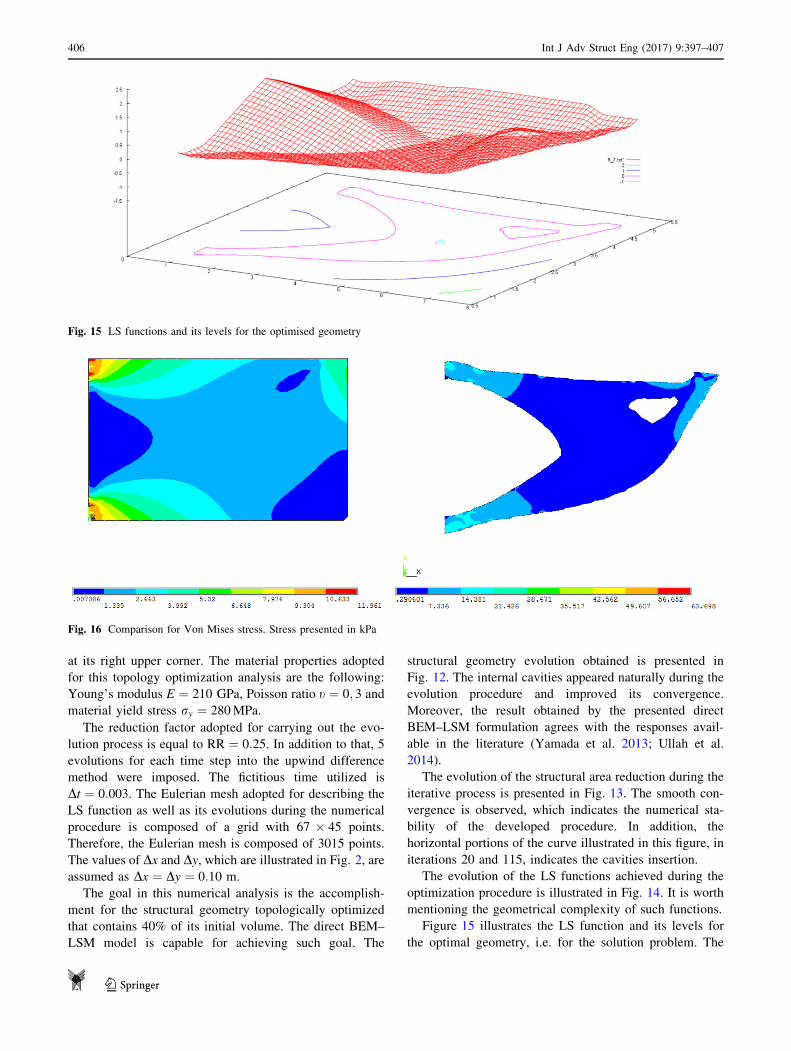
Fig. 9 LS functions and its levels for the optimised geometry

Fig. 10 Comparison for Von Mises stress. Stress presented in kPa

Fig. 11 Structure analysed. Dimensions in metre

Fig. 12 Geometry evolution process


123

Finally, the LS function as well as its levels for the

optimal geometry is illustrated in Fig. 9. The geometrical

complexity involved in this LS must be mentioned, even

for this simple application.

In addition, the stress state in the initial and the opti-

mized structural geometries was analysed. Figure 10 pre-

sents the comparison, in which the Von Mises stresses are

illustrated. One observes the better stress distribution in the

optimized structural geometry, as expected.

Cantilever beam problem

The last application of the present study deals the topology

optimization of the plane structure illustrated in Fig. 11.

This is a cantilever beam, which is clamped at two regions

along its left end and subjected to a vertical load positionedFig. 13 Structural area evolution during the optimization procedure

Fig. 14 LS functions and its evolutions during the optimization procedure


123

at its right upper corner. The material properties adopted

for this topology optimization analysis are the following:

Young’s modulus E ¼ 210 GPa, Poisson ratio t ¼ 0; 3 and

material yield stress ry ¼ 280 MPa.

The reduction factor adopted for carrying out the evo-

lution process is equal to RR ¼ 0:25. In addition to that, 5

evolutions for each time step into the upwind difference

method were imposed. The fictitious time utilized is

Dt ¼ 0:003. The Eulerian mesh adopted for describing the

LS function as well as its evolutions during the numerical

procedure is composed of a grid with 67 � 45 points.

Therefore, the Eulerian mesh is composed of 3015 points.

The values of Dx and Dy, which are illustrated in Fig. 2, are

assumed as Dx ¼ Dy ¼ 0:10 m.

The goal in this numerical analysis is the accomplish-

ment for the structural geometry topologically optimized

that contains 40% of its initial volume. The direct BEM–

LSM model is capable for achieving such goal. The

structural geometry evolution obtained is presented in

Fig. 12. The internal cavities appeared naturally during the

evolution procedure and improved its convergence.

Moreover, the result obtained by the presented direct

BEM–LSM formulation agrees with the responses avail-

able in the literature (Yamada et al. 2013; Ullah et al.

2014).

The evolution of the structural area reduction during the

iterative process is presented in Fig. 13. The smooth con-

vergence is observed, which indicates the numerical sta-

bility of the developed procedure. In addition, the

horizontal portions of the curve illustrated in this figure, in

iterations 20 and 115, indicates the cavities insertion.

The evolution of the LS functions achieved during the

optimization procedure is illustrated in Fig. 14. It is worth

mentioning the geometrical complexity of such functions.

Figure 15 illustrates the LS function and its levels for

the optimal geometry, i.e. for the solution problem. The

Fig. 15 LS functions and its levels for the optimised geometry

Fig. 16 Comparison for Von Mises stress. Stress presented in kPa


123

geometrical complexity involved in such an LS function

must be mentioned.

The stress state in the initial and the optimized structural

geometries was also analysed. Figure 16 illustrates this

comparison, in which the Von Mises stresses are presented.

As expected, the better stress distribution is observed in the

optimized structural geometry.

Conclusion

In this study, the topology optimization analysis was

accomplished in 2D structures through the direct coupling

of BEM–LSM. In such coupled numerical model, the

advantages of each method were utilized for obtaining the

optimal structural geometry. Therefore, each method is

utilized in an efficient and accurate manner. The BEM is

applied accurately for determining stress values at the

Eulerian grid points. In addition, the BEM requires only

boundary discretization. Thus, this numerical model is well

adapted for solving topology optimization problems, as

both approaches (BEM and topology optimization) require

information over the boundary for the moving boundaries

solution problem. On the other hand, the LSM enables

robustly for the curve motion modelling. Such approach is

capable of handling accurately complex curve movements,

which involves singularities, weak solutions, topology

changes and interfaces.

Two applications were considered in this study. The

results obtained in both cases are in good agreement with

the solutions presented in the literature, which indicates the

accuracy of the direct BEM–LSM formulation presented.

Moreover, smooth and stable numerical convergence were

observed, which indicates the numerical stability of the

presented optimization scheme.

In spite of its accuracy and robustness, some develop-

ments are due in course in order to improve the developed

model. Among them, it is worth mentioning the paral-

lelization of the computational code. This development

aims at improving the computational time consuming,

which at this moment may restrict large industrial

applications.

Acknowledgements Sponsorship of this research project by the Sao

Paulo Research Foundation (FAPESP), Grant number 2014/18928-2

is greatly appreciated.

Open Access This article is distributed under the terms of the

Creative Commons Attribution 4.0 International License (http://crea

tivecommons.org/licenses/by/4.0/), which permits unrestricted use,

distribution, and reproduction in any medium, provided you give

appropriate credit to the original author(s) and the source, provide a

link to the Creative Commons license, and indicate if changes were

made.

References

Allaire G, Jouve F (2008) Minimum stress optimal design with the

level set method. Eng Anal Bound Elem 32(11):909–918

Bendsøe MP (1989) Optimal shape design as a material distribution

problem. Struct Optim 1:193–202

Bendsøe MP, Kikuchi N (1988) Generating optimal topologies in

structural design using a homogenization method. Computer

Methods Appl Mech Eng 71(2):197–224

Bertsch C, Cisilino A, Calvo N (2010) Topology optimization of

three-dimensional load-bearing structures using boundary ele-

ments. Adv Eng Softw 41(5):694–704

Brebbia CA, Dominguez J (1992) Boundary elements: and introduc-

tory course. Comput Mech Publ, London

Cervera E, Trevelyan J (2005a) Evolutionary structural optimization

based on boundary representation of NURBS. Part I: 2D

algorithms. Comput Struct 83(23):1902–1916

Cervera E, Trevelyan J (2005b) Evolutionary structural optimization

based on boundary representation of NURBS. Part II: 3D

algorithms. Comput Struct 83(23):1917–1929

Eschenauer H, Kobelev V, Schumacher A (1994) Bubble method for

topology and shape optimization of structures. Struct Multidiscip

Optim 8(1):42–51

Hong HK, Chen JT (1988) Derivations of Integral equations of

elasticity. J Eng Mech 114(6):1028–1044

Marczak JR (2007) Topology optimization and boundary elements: a

preliminary implementation for linear heat transfer. Eng Anal

Bound Elem 31(9):793–802

Maute K, Ramm E (1995) Adaptive topology optimization. Struct

Multidiscip Optim 10(2):100–112

Neches CL, Cisilino A (2008) Topology optimization of 2D elastic

structures using boundary elements. Eng Anal Bound Elem

32(7):533–544

Osher S, Fedkiw RP (2003) Level set methods and dynamic implicit

surface. Springer, New York

Osher S, Sethian J (1988) Fronts propagating with curvature-

dependent speed: algorithms based on Hamilton–Jacobi formu-

lations. J Comput Phys 79:12–49

Rozvany G, Zhou M, Birker T (1992) Generalized shape optimization

without homogenization. Struct Multidiscip Optim 4(3):250–252

Sethian J (1999) Level set methods and fast marching methods:

evolving interfaces in geometry, fluid mechanics, computer

vision, and material science, 2nd edn. Cambridge University

Press, Cambridge

Shichi S, Yamada T, Suzuki A, Matsumoto T, Takahashi T (2012) A

level set-based topology optimization method using boundary

element method in three dimension. Jpn Soc Mech Eng

78:228–239

Ullah B, Trevelyan J, Matthews PC (2014) Structural optimization

based on the boundary element and level set methods. Comput

Struct 137:14–30

Xie Y, Steven G (1993) A simple evolutionary procedure for

structural optimization. Comput Struct 49(5):885–896

Yamada T, Shichi S, Matsumoto T, Takahashi T, Isakari H (2013) A

level set-based topology optimization method using 3D BEM.

Adv Bound Elem Tech XIV 1:432–437

Yamasaki S, Yamada T, Matsumoto T (2012) An immersed boundary

element method for level-set based topology optimization. Int J

Numer Methods Eng 93(8):960–988

Publisher’s Note

Springer Nature remains neutral with regard to jurisdictional claims in

published maps and institutional affiliations.


123

http://creativecommons.org/licenses/by/4.0/

http://creativecommons.org/licenses/by/4.0/

Documents

Topology optimization analysis based on the direct