Embed Size (px)
Citation preview

TitleTopological insulators and superconductors: classification oftopological crystalline phases and axion phenomena(Dissertation_全文 )
Author(s) Shiozaki, Ken
Citation 京都大学
Issue Date 2015-03-23
URL https://doi.org/10.14989/doctor.k18779
Right
Type Thesis or Dissertation
Textversion ETD
Kyoto University
Thesis
Topological insulators and superconductors:classification of topological crystalline phases
and axion phenomena
Ken Shiozaki
Department of Physics, Kyoto University
December, 2014


Abstract
This thesis presents two topics of topological insulators and superconductors. One is a classificationof topological crystalline insulators and superconductors which are topological phases protected byspace group symmetries. Another topic is a study of axion phenomena in topological phases.
Chap. 1 is an overview of topological insulators and superconductors. Topological insulators andsuperconductors are classes of topological phases of free fermions. The momentum space topologyof the Bloch and Bogoliubov de Gennes Hamiltonian characterizes topologically stable propertiesof the ground state against perturbation, leading robust low-energy gapless excitations localized atboundaries and defects of insulators and superconductors. The exploration of axion phenomena isa significant application of topological phases in which the band topology plays an essential role.
Chap. 2 gives a self-contained introduction of the band topology. We review a usual band theorywith a careful description of symmetries, which include the time-reversal symmetry, the particle-holesymmetry, and space group symmetries. The existence of an energy gap in a band structure inducesa classification of band insulators and superconductors: there are distinct classes characterized bytopological invariants that remain unchanged against smooth variations of the band structure withpreserving the energy gap.
Chap. 3 provides the complete classification of topological crystalline phases with order-twopoint group symmetries. Those symmetries include Z2 global spin flip, reflection, two-fold rotation,inversion, and their magnetic symmetries. Bulk topological insulators and superconductors, defectgapless states, and topological semimetals are discussed in a unified framework. We find that thetopological periodic table shows a periodicity in the number of flipped coordinates under the order-two spatial symmetry, in addition to the Bott periodicity in the space dimensions. We give a numberof concrete examples in Chap. 4.
The theme of Chap. 5 is about a physical implication of topological invariants. In the caseof chiral symmetric systems in odd spatial dimensions such as time-reversal invariant topologicalsuperconductors and topological insulators with sublattice symmetry, the relation between bulktopological invariants and experimentally observable physical quantities has not been well under-stood. We clarify that the winding number which characterizes the bulk Z nontriviality of thesesystems can appear in electromagnetic and thermal responses in a certain class of heterostructuresystems. It is also found that the Z nontriviality can be detected in a certain polarization inducedby magnetic field.
In Chap. 6, we argue dynamical axion phenomena in superconductors and superfluids in termsof the gravitoelectromagnetic topological action, in which the axion field couples with mechanicalrotation under finite temperature gradient. The dynamical axion is induced by relative phase fluc-tuations between topological and s-wave superconducting orders. We show that an antisymmetricspin-orbit interaction which induces parity-mixing of Cooper pairs enlarges the parameter regionin which the dynamical axion fluctuation appears as a low-energy excitation. We propose that the
1

dynamical axion increases the moment of inertia, and in the case of ac mechanical rotation, i.e. ashaking motion with a finite frequency ω, as ω approaches the dynamical axion fluctuation mass,the observation of this effect becomes feasible.
2

Contents
Abstract 1
List of publications 5
Chapter 1 Overview: topological phases of free fermions 61 Topological phases of matter . . . . . . . . . . . . . . . . . . . . . . . . . . . . . . . 62 Topological insulators and superconductors . . . . . . . . . . . . . . . . . . . . . . . 73 Topological crystalline insulators and superconductors . . . . . . . . . . . . . . . . . 84 Boundary gapless states . . . . . . . . . . . . . . . . . . . . . . . . . . . . . . . . . . 105 Defect gapless states . . . . . . . . . . . . . . . . . . . . . . . . . . . . . . . . . . . . 116 Topological fermi point . . . . . . . . . . . . . . . . . . . . . . . . . . . . . . . . . . . 157 Adiabatic pump . . . . . . . . . . . . . . . . . . . . . . . . . . . . . . . . . . . . . . . 168 Axion physics . . . . . . . . . . . . . . . . . . . . . . . . . . . . . . . . . . . . . . . . 189 Experimental realizations . . . . . . . . . . . . . . . . . . . . . . . . . . . . . . . . . 1810 Classification of topological crystalline phases with order-two point group symmetry 2011 Chiral topological phases and winding number . . . . . . . . . . . . . . . . . . . . . 2112 Dynamical axion in superconductors and superfluids . . . . . . . . . . . . . . . . . . 22
Chapter 2 Band topology 241 Bloch Hamiltonian . . . . . . . . . . . . . . . . . . . . . . . . . . . . . . . . . . . . . 242 Symmetry . . . . . . . . . . . . . . . . . . . . . . . . . . . . . . . . . . . . . . . . . . 273 Topology of gapped Hamiltonian . . . . . . . . . . . . . . . . . . . . . . . . . . . . . 354 Altland-Zirnbauer symmetry class and extension problem of Clifford algebra . . . . . 425 Dimensional shift of Hamiltonians . . . . . . . . . . . . . . . . . . . . . . . . . . . . 446 Defect Hamiltonians and dimensional hierarchy of AZ classes . . . . . . . . . . . . . 477 Topological invariants . . . . . . . . . . . . . . . . . . . . . . . . . . . . . . . . . . . 51
Chapter 3 Topological phases with order-two point group symmetry 591 Order-two point group symmetries . . . . . . . . . . . . . . . . . . . . . . . . . . . . 602 K-group in the presence of additional symmetry: additional symmetry class . . . . . 623 Dimensional hierarchy with order-two additional symmetry . . . . . . . . . . . . . . 664 Classifying space of AZ classes with additional symmetry . . . . . . . . . . . . . . . 685 Properties of K-group with an additional order-two point group symmetry . . . . . . 716 Weak crystalline topological indices . . . . . . . . . . . . . . . . . . . . . . . . . . . . 737 Topological classification of Fermi points with additional order-two point group sym-
metry . . . . . . . . . . . . . . . . . . . . . . . . . . . . . . . . . . . . . . . . . . . . 74
3

8 Conclusion . . . . . . . . . . . . . . . . . . . . . . . . . . . . . . . . . . . . . . . . . 78
Chapter 4 Periodic table in the presence of additional order-two symmetry 801 Z2 global family (δ∥ = 0) . . . . . . . . . . . . . . . . . . . . . . . . . . . . . . . . . . 802 Reflection family (δ∥ = 1) . . . . . . . . . . . . . . . . . . . . . . . . . . . . . . . . . 873 Two-fold rotation family (δ∥ = 2) . . . . . . . . . . . . . . . . . . . . . . . . . . . . . 934 Inversion family (δ∥ = 3) . . . . . . . . . . . . . . . . . . . . . . . . . . . . . . . . . . 101
Chapter 5 Electromagnetic and thermal responses of chiral topological insulatorsand superconductors 1051 Chiral symmetry and winding number . . . . . . . . . . . . . . . . . . . . . . . . . . 1052 Z2 characterization of winding number . . . . . . . . . . . . . . . . . . . . . . . . . . 1063 Bulk winding number and magnetoelectric polarization in chiral symmetric TIs . . . 1064 Case of time-reversal invariant topological superconductors . . . . . . . . . . . . . . 1085 Chiral polarization and the winding number . . . . . . . . . . . . . . . . . . . . . . . 1106 Conclusion . . . . . . . . . . . . . . . . . . . . . . . . . . . . . . . . . . . . . . . . . 111A Appendix . . . . . . . . . . . . . . . . . . . . . . . . . . . . . . . . . . . . . . . . . . 111
Chapter 6 Dynamical axion phenomena in superconductors and superfluids 1181 Introduction . . . . . . . . . . . . . . . . . . . . . . . . . . . . . . . . . . . . . . . . . 1182 Gravitational topological action term for topological superconductors . . . . . . . . . 1193 Basic features of class DIII topological superconductors . . . . . . . . . . . . . . . . 1224 Dynamical axion in TSCs with s-wave pairing interaction . . . . . . . . . . . . . . . 1245 Dynamical axion phenomena in topological superconductors . . . . . . . . . . . . . . 1306 Conclusion . . . . . . . . . . . . . . . . . . . . . . . . . . . . . . . . . . . . . . . . . 131
Chapter 7 Conclusion 132
Bibliography 134
Acknowledgment 142
4

List of publications
Published papers related to the thesis
1. Ken Shiozaki and Masatoshi SatoTopology of crystalline insulators and superconductorsPhys. Rev. B 90, 165114 (2014).
2. Ken Shiozaki and Satoshi FujimotoElectromagnetic and Thermal Responses of Z Topological Insulators and Superconductors inodd Spatial DimensionsPhys. Rev. Lett. 110, 076804 (2013).
3. Ken Shiozaki and Satoshi FujimotoDynamical axion in topological superconductors and superfluidsPhys. Rev. B 89, 054506 (2014).
Published papers not included in the thesis
4. Ken Shiozaki and Satoshi FujimotoGreen’s function method for line defects and gapless modes in topological insulators: Beyondthe semiclassical approachPhys. Rev. B 85, 085409 (2012).
5. Ken Shiozaki, Takahiro Fukui, and Satoshi FujimotoIndex theorem for topological heterostructure systemsPhys. Rev. B 86, 125405 (2012).

Chapter 1
Overview: topological phases of freefermions
In this Chapter, before presenting a detailed discussion of topological insulators and supercon-ductors, we give a basic concept of “topological phases of matter”. Topological insulators andsuperconductors are classes of topological phases of free fermions. We give an overview of the topo-logical band theory by using concrete examples in Sec. 4 - Sec. 7. The topological band theory offersa systematic description of gapless boundary states, gapless states localized at defects, topologicalfermi points, and adiabatic pumps. They are related closely to each other. Realization of the axionphysics is a significant feature of topological phases, which is briefly explained in Sec. 8. We collectsome experimental realizations of topological insulators and superconductors in Sec. 9. The lastthree sections, Sec. 10- Sec. 12 are devoted to short introductions of Chap. 3 - Chap. 6.
1 Topological phases of matter
Phases of matter are usually characterized by symmetry breaking and order parameters. Magnetism,superconductivity, and superfluidity provide fundamental examples. Consider a magnetic phasetransition with broken Z2 symmetry. In the high temperature disordered phase, the Z2 symmetryin the spin space is not broken. At the critical temperature Tc, the Z2 symmetry is spontaneouslybroken, and the system shows magnetism associated with a finite Z2 breaking order parameter.
However, there are distinguishable phases with the same symmetry and without (local) orderparameters. Such phases occur in gapped quantum phases at zero temperature. Integer quantumHall states and fractional quantum Hall states offer typical examples. Those phases indicate differ-ent characters from ordinarily phases such as existences of boundary gapless states, ground statedegeneracy depending on real-space topology, and bulk low-energy excitation with fractional chargeand statistics. [1]
A possible definition of such unusual phases is an operational one described as follows. Weconsider a family of Hamiltonians H(λ)λ∈Λ where λ represents all possible parameters in givendegrees of freedom and symmetries. The parameter space Λ is categorized into three types on aviewpoint of ground state property of H(λ) as: 1
(i-a) gapped phases without breaking symmetry,
1 Here we consider bulk quantum phases, where the energy gap from the finite size effect is neglected.
6

Figure 1.1: [a] A example of a topological phase diagram. λ1, λ2 represent the parameters ofHamiltonian. White regions A, B, C represent distinct topological phases. Red regions representgapped symmetry-broken phases or gapless phases. [b] The effect of symmetry attachment totopological phases. Topological phases may be divided into more multiple phases (A and C), ordisappeared (B).
(i-b) gapped phases with breaking symmetry,
(ii) gapless phases.
We can define an equivalence relation in (i-a) phases as follows: H1 and H2 are equivalent if and onlyif H1 can be continuously deformed into H2 without breaking the symmetry or closing the energygap. Then the gapped phases without breaking symmetry are divided into some equivalent classeswhich are separated by the gapless phases or symmetry breaking phases. The equivalent classes arereferred to as topological phases. In Fig. 1.1 [a] we show a schematic picture of a topological phasediagram.
In topological phases, symmetry plays an important role. Symmetries restrict possible formsof Hamiltonians, which gives a finer classification of topological phases. Let us consider the effectof symmetry attachment. Assume that there are topological phases A,B,C, . . . in a symmetryclass S0. Then, in the symmetry class S1 = S0 + S′, due to the restriction on parameters by thesymmetry S′, the topological phases may be divided into different phases: A 7→ A-a,A-b, A-c, . . . ,or forbidden: A 7→ empty. In Fig. 1.1 [b] we show a schematic picture of the role of symmetry intopological phases.
2 Topological insulators and superconductors
Topological insulators and superconductors [2, 3] are topological phases of free fermions, in otherwords, topological phases of one-particle states. Band insulators, superconductors and superfluids(within a mean field approximation) belong to this category. Topological insulators and supercon-ductors are the main topic of this thesis.
7

If there is the lattice translational symmetry, Hamiltonians are characterized by the BlochHamiltonians H(k) with the Bloch momentum k which is a good quantum number. Then, thecharacterization of topological phases is simplified to the homotopy classification of the map H(k)from Brillouin zone (BZ) to matrix space with a finite energy gap. [4, 5, 6] We can apply mathemat-ical tools of topology, especially the K-theory, [7, 8, 9] to the classification of topological insulatorsand superconductors. 2
Since the bulk has a finite energy gap from the ground state a signature of nontrivial topologycannot be seen in the bulk. All possible signatures of nontrivial topology occur only at real spaceboundaries of matters or interfaces between topologically distinct phases. 3 On the boundary oftopologically nontrivial insulators and superconductors there should be gapless states which arerobust against disorder and perturbation. Topological defects such as vortex and monopole defectsand edge and screw dislocations also provide gapless states which are robust against disorder. [10, 11]Also, even if there is no gapless state at the boundary due to symmetry breaking (for example, thetime-reversal symmetry breaking perturbation at the boundary, or obviously breaking of crystallinesymmetries from the existence of the boundary), some topological nontrivialities may be capturedin the variation of the charge polarization and the magnetoelectric polarization near the boundary,which leads to topologically robust electromagnetic and thermal responses. [12, 13]
Some topological invariants characterizing topological phases are directly related to experi-mentally observable quantities. For example, the Chern (TKNN) number, which characterizes2-dimensional time-reversal symmetry-broken topological phases, is nothing but the (thermal)Hall conductivity. [14, 15, 16] The 3-dimensional Chern-Simons invariant, which characterizes 3-dimensional time-reversal or inversion symmetric topological insulators, gives the topological mag-netoelectric coefficient. 4 [13] However, not all topological invariants are related to some physicalobservable quantities.
A common physical meaning of topological invariants is the “bulk-boundary correspondence”:If a bulk insulating phase shows some nontrivial topology, there should be gapless states localized atthe real space boundary. Moreover, the structure of the boundary gapless states is characterized bythe bulk topological invariant. Thus the bulk topological data are entirely reflected in the boundarygapless states. We give a concrete example in Sec. 4.
3 Topological crystalline insulators and superconductors
Crystalline symmetries are distinguished from global symmetries in topological phases. Here, crys-talline symmetries are space group symmetries which consist of spatially non-local transformation.Global symmetries are spatially local symmetries such as the time-reversal symmetry, the particle-hole symmetry, and the on-site spin SU(2) symmetry. Topological insulators and superconductors
2 The full translational symmetry is not essential for topological insulators and superconductors. The analysis of theAnderson delocalization of the boundary of topological insulators and superconductors shows the same classificationas the homotopy classification of bulk Bloch Hamiltonian H(k). [4] The present thesis does not deal with disordereffect and assume the translational symmetry when we consider a classification of topological phases.
3 For topologically ordered states (i.e., topological phases with a long-range entanglement), the bulk can show asignature of nontrivial topology via low-energy excitations with a fractional charge and statistics, which is essentiallymany-particle physics. [1] Free fermion topological phases we consider in this thesis does not show such bulk topologicalsignatures.
4 The 3-dimensional Chern-Simons invariant is also referred to as the magnetoelectric polarization or the axiontheta angle.
8

Figure 1.2: Boundary gapless states on the topological crystalline insulators. [a] For mirror reflectionsymmetry Myz, symmetry respected surfaces are y = const. and z = const. surfaces. x = const.surface is not closed under the reflection transformation. [b] For Cn rotation symmetry along z-axis,the z = const. surface is only possible symmetry respected surface.
protected by crystalline symmetries are called the “topological crystalline insulators and supercon-ductors”. [17, 18]
A physical difference between global and crystalline symmetries is stability against the disordereffects such as existence of impurities, lattice defects, and boundaries. It is naively expected that thegapless boundary modes in topological crystalline insulators and superconductors are fragile againstdisorders because these specific symmetries are microscopically sensitive to small perturbations. Butrecent studies of topological crystalline insulators have shown that if the symmetries are preservedon average, then for some symmetry classes the existence of gapless boundary states is ratherrobust. [19, 20, 21, 22] Moreover, surface gapless states protected by the mirror reflection crystalsymmetry have been observed experimentally. [23, 24, 25, 26] Such recent developments motivateus to classify the topological crystalline insulators and superconductors, and reveal their low-energyphysics.
It is required for the existence of boundary gapless states that the boundary does not breakthe crystalline symmetry. For example, consider the mirror reflection symmetry Myz : (x, y, z) →(−x, y, z). The symmetry respecting surfaces are parallel to x-axis (Fig. 1.2 [a]). Another exampleis the Cn rotation symmetry along the z-axis. The symmetry respecting surface is the z = const.plane (Fig. 1.2 [b]). The allowed space group symmetries which are compatible with the existenceof the boundary are the 2-dimensional space group symmetries in 3-dimensional materials (and sothe 1-dimensional space group symmetries in 2-dimensional materials). 5
5 The entanglement spectrum can detect topological nontrivialities for the boundary non-respecting space groupsymmetries. See, for example, [27].
9

4 Boundary gapless states
As stated previously, topological insulators and superconductors show the boundary gapless stateswhich reflect nontrivial topology of the bulk.
4.1 Example: anomalous Hall insulator
Let us illustrate the relation between bulk topology and boundary gapless states by an concretemodel known as the anomalous Hall insulator. [28] Consider a two band model in 2-dimensions,
H(kx, ky) = ε(kx, ky) +R(kx, ky) · σ, (1.4.1)
where σ = (σx, σy, σz) are the Pauli matrices. (kx, ky) stand on the 2-dimensional BZ torus T 2 =S1 × S1. The energy eigenvalues of (1.4.1) are given by
E±(kx, ky) = ε(kx, ky)± |R(kx, ky)|. (1.4.2)
We assume a finite energy gap in the overall BZ, which implies R(kx, ky) = 0 for all (kx, ky) ∈ T 2.Then we can introduce a unit vector n(kx, ky) := R(kx, ky)/|R(kx, ky)| which is not singular inT 2. The topology of the two band model is evaluated by the homotopy classification of the mapn : T 2 → S2, 6 which is characterized by the winding number
N =1
8π
∫T 2
d2kϵµνρϵijnµ∂kinν∂kjnρ. (1.4.3)
N counts how many times T 2 winds S2, 7 and is invariant under a continuous change of theHamiltonian H(k) until the bulk energy gap is closed. Hence, two band models show Z topologicalphases.
If N is a nonzero integer, there should be N chiral gapless states at the boundary. To see this,let us consider the following two orbital square lattice model with the hopping that flips the orbitals(For example, see [13]),
H =∑i
[c†i+x
σz + iσx2
ci + c†i+y
σz + iσy2
ci + h.c.]+m
∑i
c†iσzci. (1.4.4)
The Bloch Hamiltonian of (1.4.4) is
H(kx, ky) = sin kxσx + sin kyσy + (m+ cos kx + cos ky)σz, (1.4.5)
and the winding number is given by
N =
1 for − 2 < m < 0−1 for 0 < m < 20 for |m| > 2
(1.4.6)
We consider an infinite plane geometry for y > 0 as shown in Fig. 1.3 [a]. kx is a good quantumnumber since the lattice translational symmetry along x-direction is remained. In Fig. 1.3 [b-e],we show the energy eigenvalues with respect to kx for distinct values of m. In Fig. 1.3 [c] ([d]),there is a right (left) mover chiral gapless state localized at the boundary, which reflects the bulktopological invariant N = 1(−1). 8 9
6 The potential term ε(kx, ky) merely contributes an energy shift, and does not affect the topology.7 There is no winding from a sub circle S1 ⊂ T 2 to S2 since S1 cannot wind in S2.8 The right and left mover are determined by the group velocity ∂E(kx)/∂kx of the gapless states.9Strictly speaking, the bulk topology protects the difference of the number between right and left mover chiral
10
-Π Π
kx
EHkxL
-Π Π
kx
EHkxL
-Π Π
kx
EHkxL
-Π Π
kx
EHkxL
x
TI
Vacuum
[a] [b] [c]
[d] [e]
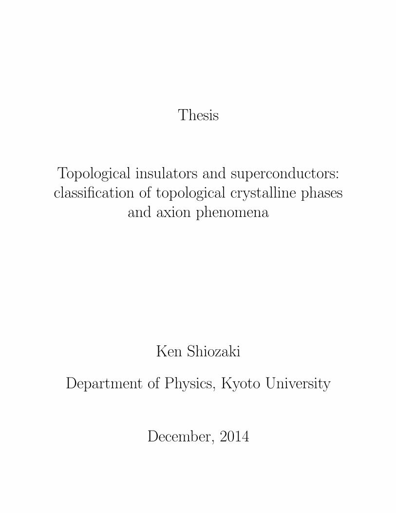
Figure 1.3: [a] The anomalous Hall insulator for y > 0 and the vacuum for y < 0. [b-e] The energyeigenvalues for the infinite plane geometry [a] with [b] m = −3, [c] m = −1, [d] m = 1, and [d]m = 3. Thick blue lines in [c] and [d] are chiral gapless boundary states localized at the interfacebetween the anomalous Hall insulator and the vacuum.
4.2 Bulk-boundary correspondence
In previous subsection, we saw the relation between the bulk topology (homotopy of H(kx, ky)) andthe existence of the chiral gapless states at the boundary. This is an example of the bulk-boundarycorrespondence, which states:
• If a bulk Hamiltonian H(k) has nontrivial topology, then there should be gapless states local-ized at the boundary which reflect the bulk topological invariant.
There are many papers about the bulk-boundary correspondence. See, [29, 30, 31], for example.
5 Defect gapless states
Topological band theory is also applied to gapless states localized at defects. Here the defects includetopological defects such as domain wall, vortex, monopole defects, and also lattice dislocations.
gapless excitations.
11

5.1 Example: Jackiw-Rossi vortex zero mode
We start up with a concrete example known as the Jackiw-Rossi model. Consider a 2-dimensionalDirac model with a single vortex: [32, 33]
H = −iγ1∂x − iγ2∂y +∆(r) cosϕ γ3 ±∆(r) sinϕ γ4 (1.5.1)
where γµ-s are Dirac matrices satisfying γµ, γν = δµν , ϕ is the azimuth angle, and we assume∆(r → ∞) → ∆0 > 0. The prefactor of the fourth term ± corresponds to the chirality of thevortex. We set γ5 = iγ1γ2γ3γ4. Due to the finite mass gap ∆0, there is no low-energy excitation farfrom the vortex, i.e., “insulator”. Near the vortex there may be discrete in-gap excitations. It isknown that the Hamiltonian (1.5.1) has a zero energy state ϕ0(x, y) localized at the vortex of whichthe wave function is
ϕ0(x, y) ∝ ξ±e±iϕe−
∫ r0 dr′∆(r′) (1.5.2)
with the fixed chirality of γ5: γ5ξ± = ±ξ± (or γ5ξ± = ∓ξ±). 10
The zero energy state ϕ0 is shifted from the zero under the perturbation such as Hpert = V orV ′γ5. If we assume the “chiral symmetry” H, γ5 = 0, those perturbations are forbidden, and weexpect the zero energy states are stable under perturbations preserving the chiral symmetry. This istrue from the following reason: Noticing [H, γ5] = 0 on the subspace spanned by zero energy statesunder the chiral symmetry, we can find that an zero energy state are also an eigen state of γ5.
11
A pair of zero energy states with positive and negative chiralities |ϕ+0 ⟩ , |ϕ−0 ⟩ can be gapped out
without breaking the chiral symmetry because of the existence of the chiral symmetry preservingperturbation α |ϕ+0 ⟩ ⟨ϕ
−0 |+ h.c., α |ϕ+0 ⟩ ⟨ϕ
−0 |+ h.c., γ5 = 0. Thus,
Ind(H) := N+ −N−, (1.5.3)
the difference between the number of positive and negative chiral zero modes, may be stable underperturbations with the chiral symmetry. Ind(H) is referred to as the analytic index of H. Morestrictly, the index theorem for the open infinite system [34, 35] states that the analytic index iscompletely determined by an certain topological index as
Ind(H) =1
2πi
∮|r|→∞
dΦ(ϕ) (1.5.4)
where the r.h.s is the total phase winding of the gap function ∆(r)eiΦ(ϕ) at the infinite regionr → ∞. 12 Thus, the number of zero energy states near the vortex does not depend on micro-scopic structure, determined only by the topological information far away from the vortex, which
10 The sign of chirality of the zero energy state depends on the definition of the gamma matrices. The essentialpoint is the one-to-one correspondence between the chirality of the phase winding ± in Eq. (1.5.1) and the chiralityof the zero energy states.
11 If |ϕ⟩ is a zero energy state, we get [H, γ5] |ϕ⟩ = −2γ5H |ϕ⟩ = 0.12 The assumptions on the index theorem (1.5.4) are
• (i) The Dirac theory
• (ii) The existence of the chiral symmetry H,Γ = 0
• (iii) |∆(r)| > 0 for r → ∞However, the condition (iii) can be weaken to
12

is symbolically written as
Analytic index = Topological index. (1.5.5)
This is the same spirit as the bulk-boundary correspondence.
5.2 Bulk-defect correspondence
It is suggested that the index theorem (1.5.4) is generalized to non Dirac systems such as latticesystems or Hamiltonians including higher order derivatives, and also for any symmetry classes.The generalized conjecture is known as the “bulk-defect correspondence” [10] explained below. LetH(k, r) be a Hamiltonian describing a defect. The momentum and position operators k and r donot commute because the translation symmetry is broken due to the defect. We assume that thereis no gapless excitation far from the defect. We set a closed sphere SD surrounding the defect,where (D+ 1) is the defect co-dimensions. For example, in the case of the point defect in 2-spatialdimensions as given by (1.5.1), the defect surrounding sphere is the circle S1. Without loss ofgenerality, we can assume that ξvar, which is the characteristic length of the spatial variation of thedefect Hamiltonian on the sphere SD, is sufficiently slower than ξgap: ξvar ≪ ξgap, where ξgap is thecharacteristic length determined by the finite energy gap far from the defect. This simplificationimplies that the semiclassical Hamiltonian on the sphere H(k, s) := H(k, r(s)) is fully gapped. 13
The semiclassical Hamiltonian H(k, s) defines the map from the base space T d×SD to the “space ofgapped Hamiltonian matrices”, which is a similar situation to the bulk-boundary correspondence.The bulk-defect correspondence says:
• If a semiclassical Hamiltonian H(k, s) is topologically nontrivial, then there should be gaplessstates localized at the defect. Also, the structure of the gapless states reflects the topologicalinvariants of the semiclassical Hamiltonian H(k, s).
5.3 Defect gapless state as a boundary gapless state
Actually, the topological classification of defect gapless states is reduced to the classification ofboundary gapless states. 14
For example, let us consider the classification of zero energy bound states localized at a pointdefect in 3-dimensions with a symmetry class S. The topological classification is determined by thehomotopy classification of symmetry compatible Hamiltonians H3D(kx, ky, kz, θ, ϕ) where (θ, ϕ) arethe parameters for a sphere S2 surrounding a point defect. The K-theory classification shows thetopological classification ofH3D(kx, ky, kz, θ, ϕ) is the same as that of the one-lower dimensional sub-system; i.e. the classification of zero energy states localized at a point defect in 2-dimensions with
• (iii’) There is no gapless excitation at r → ∞,
which allows the vortex Hamiltonian H to be more complicated systems such as heterostructure systems. [35, 36]Moreover, any systems satisfying the condition (iii’) is adiabatically (i.e., without closing the finite energy gap atr → ∞) changed into a Hamiltonian satisfying the condition (iii). As a result, without loss of generality, we canassume the condition (iii) for defect gapless states. [11, 36]
13 Even if the condition ξvar ≪ ξgap is not satisfied, the Hamiltonian H(k, r) can be adiabatically changed intothat satisfying this condition. This is justified by a way similar to the footnote 12. The Hamiltonian on the sphereH(k, s) is also referred to as the adiabatic Hamiltonian. [11]
14 Strictly speaking, this reduction is true for so called “strong indices” which represent topological nontrivialityover the base space of the one-point compactification T d × SD → Sd+D.
13

t
t
D=1
D=0
D=2
d=1 d=2 d=3[a] [b]
××
Vortex zero modes
Phase winding at far from vortices
Figure 1.4: [a] The number of vortex zero modes is determined by the phase winding at far fromthe vortices. [b] Various defect gapless states. d is the space dimensions and (D + 1) is the defectcodimensions. A defect with codimension (D + 1) is enclosed by a D-dimensional sphere SD. Thesame background color regions (the same defect dimensions d−D−1) indicate the same topologicalclassifications. [6, 11]
the same symmetry class S, of which the semiclassical Hamiltonian is H2D(kx, ky, ϕ) where ϕ is theparameter for a circle S1 surrounding the defect. Furthermore, the classification of H2D(kx, ky, ϕ)is the same as the classification of zero energy states localized at a point defect in 1-dimension withthe same symmetry class S, i.e., boundary gapless states of 1-dimensional insulators, H1D(kx).
We can always iterate such reduction to a lower-dimensional sub-system up to a boundarystate of a (D + 1) dimensional insulator with the same symmetry class S. In other words, thetopological classification of defect gapless states with a defect dimension (d,D), where d is a spatialdimension and (D + 1) is a defect co-dimension, is determined only by the defect dimension itselfδ − 1 = d−D − 1. [6, 11]
We summarize the above discussion by the following statement dubbed “a defect gapless stateas a boundary state”: [37]
• The topological classification of defect gapless states localized at a (δ− 1)-dimensional defectis the same as the topological classification of boundary gapless states of a δ-dimensionalinsulator with the same symmetry class. 15
15 If a symmetry class S includes a crystalline symmetry, it is required for the topological protection of gaplessstates that the δ-dimensional insulator, of which the boundary composes the (δ − 1)-dimensional defect, is invariantunder the crystalline symmetry transformations. [38] Note that the invariance of the (δ− 1)-dimensional defect underthe crystalline symmetry does not imply topological protection of the gapless states. We will discuss this point indetail in Sec. 5.2 of Chap. 3.
14

Figure 1.5: Fermi singularities (red regions) and each subspaceM surrounding the fermi singularity.[a] A fermi surface and two points M ∼= Z2. [b] A line node and M ∼= S1. [c] A point node andM ∼= S2.
6 Topological fermi point
The idea of band topology is also applicable to gapless phases with a nontrivial topological chargein the momentum space. [39, 10] Fermi points, lines, and surfaces are singularities of a HamiltonianH(k) in the BZ. Here the singularity means det[H(k)] = 0. At the singular point, the energy gapof the Hamiltonian H(k) should be closed, which breaks the construction of topological invariantsover all around the BZ. However, we can define topological invariants over a closed subspace Mwhich surrounds the fermi point, or general singular regions 16 where the Hamiltonian H(k) is non-singular on M . Nontrivial topology over the closed subspace M indicates the existences of a stablefermi point inner-side, and also outer-side regions of M . 17 Fig. 1.5 shows a fermi surface ([a]), aline node ([b]), a point node ([c]), and their corresponding subspaces M .
6.1 Example: Weyl semimetal
A famous example is the Weyl semimetal or the Weyl superconductor of which the fermi pointis protected by the first Chern number ch1 over the sphere S2 surrounding the fermi point. Thelow-energy effective model around the fermi point of the Weyl fermions is written as
H(k) = kxσx + kyσy + kzσz (1.6.1)
The closed sphere S2 surrounding the fermi point (k = 0) is given by |k| = k. On the sphere S2,the Hamiltonian H(k)||k|=k is fully gapped, thus we can define the first Chern number
ch1 =i
2π
∫S2
trF , (1.6.2)
16 In the presence of symmetries, the subspace M have to be closed under the symmetry group transformations.17 This is essentially the Nielsen-Ninomiya no go theorem. [39] On the other hand, if a momentum space is open,
the nontrivial topology on M indicates the existence of a stable fermi point only inner-side of M . An example wherethe momentum space is open is the Dirac theory of which the Bloch Hamiltonian is given by H(k) = γ1k1+ · · ·+γdkd.
15

where F is the Berry curvature of the occupied state of the Hamiltonian H(k) on S2. We can showch1 = −1 for the Weyl fermion (1.6.1), which implies the existence of a stable fermi point inner-sideof S2, i.e. the Weyl point.
7 Adiabatic pump
Consider a time-dependent Hamiltonian H(t) which has a finite energy gap ∆ between the groundstate and the first excited state. If the time dependence of H(t) is much slower than 1/∆, we cantake the adiabatic approximation for time evolution of the ground state. Let L = ℓ(s) ∈ Λ|0 ≤s ≤ 1, ℓ(0) = ℓ(1) be a loop in the parameter space Λ of the Hamiltonian. Correspondingly, we geta time-dependent Hamiltonian H(t) := H(ℓ(t/T )) (0 ≤ t ≤ T ) with H(T ) = H(0). The adiabaticcycle is defined by a limit T → ∞ for the fixed loop L.
The Thouless adiabatic charge pump [40] is the integrated conserved current during an adia-batic cycle. The adiabatic charge pump is quantized into an integer value and it is topologicallyrobust against perturbation. The topological band theory provides the classification of such topo-logical adiabatic charge pump in insulators. The fermion parity pump during an adiabatic cycle insuperconductors are also characterized by the topological band theory. [11]
In this thesis, we do not deal with the adiabatic pump. However, the adiabatic pump is asignificant notion in topological phases since the adiabatic charge pump is related to the bulk-boundary correspondence (Ex. [13]), and the adiabatic fermion parity pump is related to the non-abelian statistics of the Majorana fermions. [11] In the following, we briefly illustrate the adiabaticcharge pump by using a concrete example.
7.1 Example: adiabatic charge pump
We give an example of the adiabatic charge pump. [40] Consider the following 1-dimensional spinlessmodel as shown in Fig 1.6 [a], 18
H =∑i
( t2a†iai+1 +
δ
2(−1)ia†iai+1 + h.c.
)+∑i
∆(−1)ia†iai. (1.7.1)
In the bulk with the translational symmetry, the Bloch Hamiltonian is written by
H(kx) = t cos(kxa)σx − δ sin(kxa)σy +∆σz, kx ∈ [− π
2a,π
2a] (1.7.2)
with the boundary condition in the BZ H(π/2a) = σzH(−π/2a)σz. Here t is the hopping, δ is thebond order, ∆ is the staggered potential, σ = (σx, σy, σz) are the Pauli matrices for even and oddsites, and a = xi+1 − xi.
19 The energy eigenvalues of (1.7.2) are given by
E±(kx) = ±√t2 cos2(kxa) + δ2 sin2(kxa) + ∆2. (1.7.4)
18This model is known as the Rice-Mele model. [41]19 Here we chose the Fourier transformation as
a2i =∑
− π2a
<kx< π2a
ae,kxeikxx2i , a2i+1 =
∑− π
2a<kx< π
2a
ao,kxeikx(x2i+a).
(1.7.3)
16
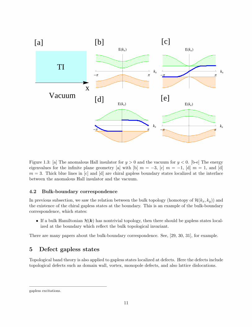
Figure 1.6: [a] The Rice-Mele model. [b] An adiabatic cycle which indicates a topological chargepump.
Thus the gapless parameter regions in the space (t, δ,∆) are given by (t, 0, 0) and (0, δ, 0). Notethat the spatial parameters (t, δ = ±t,∆ = 0) and (0, 0,∆) show the flat bands composed of thelocalized orbitals.
Let us consider the following adiabatic cycle (i) → (ii) → (iii) → (iv) → (i) as shown in Fig. 1.6[b]:
(i) t = δ = 0, ∆ > 0: localized at the even site.
(ii) t+ δ = 0,∆ = 0: localized at the (2i− 1)− (2i) bond.
(iii) t = δ = 0, ∆ < 0: localized at the odd site.
(iv) t− δ = 0,∆ = 0: localized at the (2i)− (2i+ 1) bond.
Under the above cycle, the system returns to the initial, but there is a charge pumping from theleft to the right unit cell, as shown in Fig 1.6 [b]. More generally, a pumped fermion number iscomputed by the integral of the adiabatic current [42, 40, 43]
Jad(τ) = 2a
∫BZ
dkx2π
jad(kx, τ) =2a
2π
∫ π2a
− π2π
dkx
[∂E−(kx, τ)
~∂kx− iFkxτ (kx, τ)
](1.7.5)
where τ is the adiabatic parameter labeling the adiabatic process and Fkxτ is the Berry curvatureof the occupied bands of the adiabatic Hamiltonian H(kx, τ). The pumped fermion number par an
17

adiabatic cycle is
N =1
2a
∮dτJad(τ) = − i
2π
∫dkxdτFkxτ (kx, τ) = −ch1. (1.7.6)
Here ch1 is the first Chern number which is a topological invariant and does not depend on mi-croscopic structure of the adiabatic cycle. The first Chern number ch1 reflects the topology of theadiabatic Hamiltonian H(kx, τ), and determines the pumped fermion number at the adiabatic cycle.
8 Axion physics
The axion was introduced as a hypothetical particle to resolve the strong CP problem in quan-tum chromodynamics. The axion field θ is a pseudoscalar under the time-reversal and the paritytransformation, and may couples to the electromagnetic field via the action,
Stop =α
4π2
∫d3xdtθ(x, t)E ·B. (1.8.1)
Here α = e2/~c is the fine structure constant. Because α4π2~
∫d3xdtE · B = N is a topological
invariant which does not depend on a detail of the electromagnetic field, the axion field θ(x) takesvalues in a circle S1, 20 and a constant axion field θ(x, t) = θ0 cannot contribute dynamics. Aspatially or temporally inhomogeneous background axion field or a fluctuation of the axion fieldshow meaningful effects. The electrodynamics associated with the axion field is called the axionelectrodynamics. [44]
Some topological insulators provide the axion electrodynamics. In the bulk we can define thestatic axion field θ for a given insulator by
θ =1
4π
∫tr[AdA+
2
3A3]
(mod 2π) (1.8.2)
where A(k) is the Berry connection of the Bloch Hamiltonian H(k). The time-reversal symmetryor the inversion symmetry quantizes θ by 0 or π because the axion field θ is a pseudoscalar. Infact, in the presence of these symmetries the axion field θ is nothing but the topological invariantcharacterizing the topological phases of the bulk insulators. Consider an interface between θ = 0and θ = π phases. If there is no gapless excitation at the interface due to symmetry breakingperturbation, θ is changed from 0 to π without singularity, which leads to the quantum Hall effectand the Kerr rotation from the action (1.8.1). [13]
Thermal and quantum fluctuations of the axion field θ also yield various interesting phenomena.It is proposed that some magnetic fluctuations induce the dynamical axion field, which leads to theaxionic polariton under an applied magnetic field [45] and a magnetic instability under an appliedelectrostatic field. [46]
9 Experimental realizations
In this section we collect experimental realizations of topological insulators and superconductorsand gapless topological phases.
20Note that exp(
i~Stop[θ + 2π]
)= exp
(i~Stop[θ]
).
18

9.1 Integer quantum Hall effect
A familiar example of topological insulators is the integer quantum Hall effect, [47] where the Hallconductivity σH shows plateaus along increasing an applied magnetic field, and is quantized intointeger values σH = e2
h N . The quantized σH is nothing but the topological invariant characterizingthe ground states.
9.2 Quantum spin Hall effect
After the theoretical discovery of the quantum spin Hall effect by Kane and Mele [48, 49], it wasproposed that a HgTe quantum well shows the quantum spin Hall effect [50], and experimentallyobserved. [51]
9.3 Time-reversal symmetric Z2 topological insulators
The parity criterion of time-reversal symmetric Z2 topological insulators with the inversion symme-try [52] provides a useful way to determine Z2 topological invariant for various realistic materials,and a good scenario of topological phase transition, i.e., a band inversion at symmetric points. Aftera theoretical proposal, [52] a surface Dirac fermion is observed by the Angle-resolved photo emissionspectroscopy (ARPES) measurement in Be1−xSbx. Various materials have been confirmed to be3-dimensional Z2 topological insulators. See, for example, Ando [53].
9.4 Time-reversal symmetric topological superconductor and superfluid
3-dimensional time-reversal symmetric superconductors and superfluids are classified by Z. A non-trivial phase with n ∈ Z topological invariant shows n number of surface Majorana fermions. It isknown that 3He-B phase is a topological superfluid with n = 1. [54, 4] The CuxBe2Se3 supercon-ductor is a candidate for a topological superconductor [55, 56]
9.5 Time-reversal broken topological superconductor in 2D
Topological nontriviality in 2-dimensional superconductors requires the broken time-reversal sym-metry. A topologically nontrivial phase shows chiral gapless Majorana fermions at the boundary.More interestingly, vortex zero modes of topological superconductors with the odd Chern numberindicates non-abelian braiding statistics [37, 57] which may serve as qubits for quantum computa-tion. [58, 59] Sr2RuO4 is a promising candidate for a 2-dimensional chiral superconductor. [60]
9.6 Topological crystalline insulator with mirror symmetry
3-dimensional Z2 topological insulators have odd number of surface Dirac fermions. Even number ofsurface Dirac fermions are not stable against nonmagnetic disorder which may induce a scatteringbetween a pair of Dirac fermions. However, crystalline symmetry may forbid such gap-generatingscattering term. In fact, the mirror symmetry with the time-reversal symmetry shows Z topologicalclassification, and a n ∈ Z phase indicates stable 2n number of surface Dirac fermions. [17] This isan example of topological crystalline insulators. [18]
After the proposal that SeTe shows a nontrivial topological crystalline insulator with the mirrorsymmetry [23], a pair of surface Dirac fermions is experimentally observed [24, 25, 26].
19

9.7 Dirac semimetals
Dirac semimetals are 3-dimensional analog of graphene. There is a gapless Dirac fermion in thebulk which has a nontrivial topological charge and is stable against disorder. The Dirac semimetalsoffer a platform for engineering other exotic phases such as Weyl semimetals, axion insulators, andtopological superconductors. Recently, Na3Bi [61] and Cd3As2 [62, 63, 64] were experimentallyconfirmed as the Dirac semimetals.
9.8 Weyl superconductor and superfluid
Weyl semimetals and superconductors/superfluids have a pair of stable point nodes with the firstChern number in the BZ. Weyl semimetals have not yet been found experimentally. The 3He-Aphase is known as a Weyl superfluid. [10] A superconducting phase of URu2Si2 is a candidate fora time-reversal broken chiral superconductor, [65, 66] indicating a Weyl superconductor with thetopological charge ch1 = 2 for each point node.
10 Classification of topological crystalline phases with order-twopoint group symmetry
The classification of topological crystalline insulators and superconductors for general space groupsymmetries is a difficult issue. There are 230 distinct space group symmetries in three spatial dimen-sions, which implies 230 distinct problems in the topological classification. Moreover, by combiningwith the time-reversal symmetry and the particle-hole symmetry, possible symmetry classes increasein each element of space group symmetries. The 1651 magnetic space group symmetries are partsof possible symmetry classes. An algorithmic way to classify the topological phases for generalcrystalline symmetries is not yet known.
In the cases of order-two (magnetic) point group symmetries, we can systematically classifytopological phases. [38] In Chap. 3, we give a detailed description of this topic. The order-twopoint group symmetries include Z2 global, mirror reflection, two-fold rotation, inversion, and theirmagnetic point group symmetries. See Fig. 1.7. A peculiarity of the order-two point group symme-tries is that Hamiltonians which are compatible with the order-two point group symmetries can berepresented by the Dirac Hamiltonians,
H(k1, . . . , kd) =
d∑µ=1
kµγµ +mγd+1, (1.10.1)
as explained below. Let us consider an order-two point group transformation U which flips d∥coordinates:
U : (x1, . . . , xd∥ , xd∥+1, . . . , xd) 7→ (−x1, . . . ,−xd∥ , xd∥+1, . . . , xd). (1.10.2)
If there is an additional Dirac matrix Γ which satisfies the following conditions:
Γ, γµ = 0, (µ = 1, . . . , d∥),
[Γ, γµ] = 0, (µ = d∥, . . . , d+ 1),(1.10.3)
20

Figure 1.7: Order-two point group symmetries: [a] global Z2, [b] reflection, [c] two-fold rotation, [d]inversion.
the order-two point group symmetry U is represented by the Dirac Hamiltonian as
ΓH(k1, . . . , kd∥ , kd∥+1, . . . , kd)Γ−1 = H(−k1, . . . ,−kd∥ , kd∥+1, . . . , kd). (1.10.4)
The above observation suggests that the classification problem of topological phases with order-twopoint group symmetries can be replaced by a problem only in terms of the Dirac matrices. In fact,this expectation is true, which is explained in Chap. 3. The replaced problem can be systematicallysolved as the extension problem of the Clifford algebras. [5, 67, 68, 38]
We find that the topological periodic table shows a novel periodicity in the number of flippedcoordinates under the order-two point group symmetry, in addition to the Bott-periodicity in thespace dimensions. Various symmetry protected topological phases and gapless modes will be identi-fied and discussed in a unified framework. In addition, we also present a topological classification ofFermi points in the crystalline insulators and superconductors. The bulk topological classificationand the Fermi point classification show the bulk-boundary correspondence in terms of the K-theory:
Classification of bulk topological phases in (d+ 1) dimensions
⇐⇒ Classification of stable fermi point in d dimensions.(1.10.5)
In Chap. 4, we give the periodic tables with an additional order-two point group symmetry, andillustrate how the topological tables work by using concrete examples.
11 Chiral topological phases and winding number
The relation between bulk topological invariants and experimentally observable physical quantitiesis a fundamental issue of topological phases. For instance, the first Chern number appears asthe quantized Hall conductivity in the quantum Hall effect [14], and the Z2 invariant of a time-reversal invariant topological insulator in 3-dimensions can be detected in axion electromagneticresponses [13].
21

However, for the case of topological phases characterized by Z invariants in odd spatial dimen-sions, this point has not yet been fully understood. These classes include time-reversal symmetrybroken topological insulators with sublattice symmetry in one and 3-dimensions (class AIII), time-reversal invariant topological superconductors in 3-dimensions (class DIII, e.g. 3He, CuxBi2Se3 [69,56], Li2Pt3B [70]), and time-reversal invariant topological insulators and superconductors of spin-less fermions in 1-dimension (class BDI, e.g. Su-Schrieffer-Heeger model [71], Kitaev Majoranachain model [72]). It is noted that all of these classes possess the chiral symmetry (the sublatticesymmetry); i.e. the Bloch and BdG Hamiltonian H(k) satisfies the relation
ΓH(k)Γ−1 = −H(k) (1.11.1)
with Γ a unitary operator. This implies that if |ψ(k)⟩ is an eigen state of H(k) with an energyE(k), then, Γ|ψ(k)⟩ is also an eigen state with an energy −E(k). The chiral symmetry is indeedthe origin of the bulk Z topological invariant referred to as the winding number:
N1 =1
4πi
∫BZ
tr Γ[H−1dH], for 1 dimension,
N3 =1
48π2
∫BZ
tr Γ[H−1dH]3, for 3 dimensions.
(1.11.2)
A chiral symmetric topological insulator with the winding number N possesses N flavors of gaplessDirac (Majorana) fermions at the boundary, which are stable against impurity scatterings as longas the chiral symmetry is preserved. A general framework which relates the winding number toelectromagnetic or thermal responses is still lacking, and desired.
In Chap. 5, we present two approaches for the solution of this issue. One is based on the ideathat the winding number can be detected in electromagnetic and thermal responses of a certain classof heterostructure systems. We clarify the condition for the heterostructure systems in which theZ non-trivial character of the bulk systems can appear. The other one is to introduce a novel bulkphysical quantity which can be directly related to the winding number. This quantity is referred toas “chiral charge polarization”. We show that for 3-dimensional class AIII topological insulators,the chiral charge polarization is induced by an applied magnetic field, which is an analogy withtopological magnetoelectric effect.
12 Dynamical axion in superconductors and superfluids
In Chap. 6, we argue a possibility of dynamical axion phenomena in superconductors and superfluids.The dynamical axion is fluctuating field which varies the (thermal) magnetoelectric polarization(1.8.2) of the BdG Hamiltonian HBdG(k). To vary the magnetoelectric polarization θ, both thetime-reversal symmetry and the inversion symmetry have to be broken. For example, in the case ofa 3He-B phase like time-reversal invariant p-wave topological superconductor, the imaginary s-wavesuperconducting fluctuation induces the dynamical axion field. [73] For centrosymmetric crystals,such an inversion-symmetry-breaking fluctuation survives only in the narrow parameter region wherethe magnitude of the even and odd parity channel attractive interactions are close to each other.If there is an inversion-symmetry-breaking spin-orbit interaction from noncentrosymmetric crystalstructure, the dynamical axion is more feasible since the parity-mixing of Cooper pairs enables arelative phase fluctuation (Leggett mode [74]) between the even and odd parity superconductingorders.
22

In the case of superconductors and superfluids, since charge is not conserved, it is difficult todetect topological characters in electromagnetic responses. However, thermal responses can be goodprobes for topological nontriviality because energy is still conserved. A proposed action describingthe thermal axion phenomena is the following gravitoelectromagnetic θ term, [75, 76]
Sθ =πk2BT
2
12h
∫d3xdtθ(t,x)EE ·BE , (1.12.1)
where EE and BE couple with the “energy polarization” [76] and the “energy magnetization” [77],respectively. The topological action (1.12.1) describes a thermal topological magnetoelectric effect,
i.e., the energy magnetization induced by the gravitational field: ME = θπk2BT 2
12h EE , and the energy
polarization induced by the gravitomagnetic field; PE = θπk2BT 2
12h BE . [76]We consider dynamical axion phenomena in superconductors and superfluids in three spatial
dimensions in terms of the gravitoelectromagnetic topological action (1.12.1), in which the axionfield couples with mechanical rotation under finite temperature gradient. [76] We propose that thedynamical axion increases the moment of inertia, and in the case of ac mechanical rotation, i.e. ashaking motion with a finite frequency ω, as ω approaches the dynamical axion fluctuation mass,the observation of this effect becomes feasible.
23

Chapter 2
Band topology
In this chapter, we collect some mathematical formulations and basic results of the classification offree fermion topological phases. We introduce the Bloch and Bogoliubov-de Gennes (BdG) Hamil-tonian for free fermions. Symmetry plays a central role for topological classifications. We formulatesymmetry transformations of the time-reversal symmetry (TRS), the particle-hole symmetry (PHS),the chiral symmetry (CS), and space group symmetries. We illustrate the K-theory [7, 8, 9] de-scription of the band topology for class A (no symmetry) systems, and comment on the K-theorywith symmetries. We give the topological classification for the Altland-Zirnbauer (AZ) symmetryclasses (TRS, PHS, and CS) [78] by using the Clifford algebra and the suspension isomorphism ofthe K-theory. Finally, we give the topological periodic table and analytic formulae for topologicalinvariants.
1 Bloch Hamiltonian
1.1 Free fermion
Let |i⟩i∈I be a basis of a one-particle Hilbert space, and ψ†i /ψi be the associate complex fermion
creation/annihilation operators of one-particle states |i⟩. A general Hamiltonian H is written as
H =∑ij∈I
ψ†iHijψj +
1
4
∑ijkl∈I
ψ†iψ
†jVij,klψlψk + · · · . (2.1.1)
Our interest is free fermions. A Hamiltonian of free fermions is described by a quadratic form:
H =∑ij∈I
ψ†iHijψj , (2.1.2)
where Hij satisfies the hermite condition H∗ij = Hji. We also consider superconductors and super-
fluids. Within the mean field approximation, a Hamiltonian is given by
H =∑ij∈I
ψ†iHijψj +
1
2
∑ij∈I
ψ†i∆ijψ
†j +
1
2
∑ij∈I
ψi∆∗jiψj (2.1.3)
with ∆ij the gap function. ∆ij satisfies ∆ij = −∆ji from the fermion anticommutation relation
ψi, ψj = ψ†i , ψ
†j = 0. If we introduce the Nambu spinor Ψi by
Ψi =
(ψi
ψ†i
), (2.1.4)
24

Figure 2.1: Degrees of freedom within a unit cell. α, β, . . . represent the positions of atoms.i, j, . . . represent the internal degrees of freedom inner-side of an atom.
the Hamiltonian is written as
H =1
2
∑ij∈I
Ψ†i [HBdG]ijΨj + const. (2.1.5)
where
[HBdG]ij =
(Hij ∆ij
∆∗ji −Hji
)=
(Hij ∆ij
[∆†]ij −[HT ]ij
)(2.1.6)
is the BdG Hamiltonian.
1.2 Bloch and BdG Hamiltonian
Let us move on to crystalline systems. Let |Rαi⟩ be one-particle states of a crystal. R ∈ BL ∼= Zd
represents a center of unit cells which are elements of the Bravais lattice (BL). Here d is the spacedimensions. Concretely, R =
∑dµ=1 nµaµ with nµµ=1,...d ∈ Zd and aµ the lattice vectors. α labels
a localized position of atoms in a unit cell, and i expresses internal degrees of freedom inner-side ofa α-atom, such as spin, orbital, and Nambu degrees of freedom. See Fig. 2.1. The quadratic formH is a matrix in the space spanned by the basis |Rαi⟩. The lattice translation symmetry of thecrystal means Hαi,βj(R,R
′) = Hαi,βj(R+a,R′ +a) with the lattice vector a ∈ BL, which impliesHαi,βj(R,R
′) = Hαi,βj(R−R′). The good quantum number associated with the lattice translationsymmetry is called the Bloch wave number or momentum k.
To transform into the momentum space we introduce the Fourier transformation as
|kαi⟩ =∑
R∈BL
eik·(R+xα) |Rαi⟩ , (2.1.7)
where xα is localized position of the α-atom in a unit cell. |kαi⟩ is periodic in Brillouin zone (BZ)up to a phase factor depending on α:
|k +Gαi⟩ = eiG·xα |kαi⟩ (2.1.8)
25

whereG is a reciprocal lattice vector which is generated by the basis Gµµ=1,...,d satisfyingGµ·aν =2πδµν . Correspondingly, the Hamiltonian is
H = Ω
∫BZ
ddk
(2π)dψ†αi(k)Hαi,βj(k)ψβj(k), (2.1.9)
where Hαi,βj(k) is the Bloch Hamiltonian which satisfies the following periodicity in the BZ,
Hαi,βj(k +G) = e−iG·xαHαi,βj(k)eiG·xβ . (2.1.10)
The BZ is the d-dimensional torus for the Bravais lattice BL. Ω =∏d
µ=1 aµ, (aµ = |aµ|) is thevolume of a unit cell.
For superconductors and superfluids, we introduce the Nambu spinor of the momentum space,
Ψαi(k) =∑R∈Π
Ψαi(R)e−ik·(R+xα) =∑R∈Π
(ψαi(R)
ψ†αi(R)
)eik·R =
(ψαi(k)
ψ†αi(−k)
). (2.1.11)
The BdG Hamiltonian is written as
HBdG(k) =
(H(k) ∆(k)∆†(k) −HT (−k)
). (2.1.12)
1.2.1 Periodic basis
For dealing with the band topology, it is sometimes useful to introduce the periodic basis |kαi⟩′defined by
|kαi⟩′ =∑
R∈BZ
eik·R |Rαi⟩ . (2.1.13)
Of course, this basis does not take into account localized positions of α-atoms. More concretely,(2.1.13) corresponds to a different system S′ from the original system. The system S′ is given bythe translations of the position of α-atoms as xα 7→ 0. In the momentum space, this translationsare written by the following k-dependent unitary transformation
Hαi,βj(k) = e−ik·xαH′αi,βj(k)e
ik·xβ . (2.1.14)
By definition, the periodic basis |kαi⟩′ satisfies the periodicity condition
|k +Gαi⟩′ = |kαi⟩′ , (2.1.15)
H′αi,βj(k +G) = H′
αi,βj(k). (2.1.16)
Hamiltonians have the same form as (2.1.9),
H = Ω
∫BZ
ddk
(2π)dψ′†αi(k)H
′αi,βj(k)ψ
′βj(k). (2.1.17)
The classification of band topology is given by the (stable) homotopy classification of maps H(k)from the BZ (or a closed subspace) to some matrix space. Since the homotopy classification doesnot change under the unitary transformation (2.1.15), it is useful to choose the periodic basis |kαi⟩′in advance.
26

2 Symmetry
Symmetry plays an essential role in band topology. Symmetries restrict the forms of the BlochHamiltonians H(k), which changes the homotopy classifications. Symmetries are divided into globaland crystalline symmetries. The global symmetries are non-spatial symmetries which act only onlocal internal degrees of freedom i and do not act on R and α. Examples of the global symmetriesinclude the time-reversal symmetry (TRS), the particle-hole symmetry (PHS), and the global spinSU(2) symmetry. On the other hand, the crystalline symmetries are spatial symmetries whichtransform localized positions, i.e., R and α. The crystalline symmetries are specified by the spacegroup symmetries or magnetic space group symmetries. 1
2.1 Altland-Zirnbauer symmetry class
The existence of global symmetry divides a Hilbert space into the direct sum of irreducible represen-tations of the symmetry group. Here we assume the global unitary symmetries, such as the SU(2)spin symmetry, are already diagonalized, and we consider remaining symmetries in irreducibleblocks. The remaining symmetries are antiunitary symmetry or anti-symmetry which exchangesthe occupied and unoccupied states. Those symmetries form the Altland-Zirnbauer (AZ) ten-foldsymmetry classes, as explained below. [78, 79]
2.1.1 Time-reversal symmetry
A time-reversal transformation is defined in the second quantized formalism by an antiunitarytransformation
TψiT† = [UT ]ijψj , T iT
† = −i (2.2.1)
with a unitary matrix [UT ]ij , UTU†T = U †
TUT = 1. Here we suppressed the degrees of freedom R, αbecause the time-reversal transformation does not change them. TRS is an order-two symmetry,which implies that T 2 is a pure phase factor T 2 = z = eiθ in the Fock space. Due to the anti-linearityof T , we give
zT = T 3 = T z = z∗T, (2.2.2)
thus z is real z = ±1. The existence of the TRS means T HT † = H. For free fermions, the TRS iswritten as U †
TH∗UT = H. In the Bloch basis ψαi(k) =∑
R ψαi(R)e−ik·(R+xα), the momentum k is
flipped by anti-linearity of T , so we get
TH(k)T−1 = H(−k), T = UTK, T 2 = ±1. (2.2.3)
Basic examples of T 2 = ±1 are a half integer spin system and an integer spin systems. For aspin 1/2 system the time-reversal transformation is T = isyK where sy is the y-component of thePauli matrices for the spin space and K represents the complex conjugate. For a spinless systemthe time-reversal transformation is T = K.
1 The magnetic space group symmetries are combined symmetries with the time-reversal transformation and aspace group transformation
27

2.1.2 Particle-hole symmetry
The PHS is associated with the BdG Hamiltonians. First, we argue the properties of the PHS forthe Hamiltonians without pairing terms, i.e., H =
∑ψ†iHijψj . The particle-hole transformation is
defined in the second quantized formalism as a unitary transformation that changes creation andannihilation operators as
CψiC† = [UC ]
∗ijψ
†j , CiC† = i (2.2.4)
with a unitary matrix [UC ]ij , UCU†C = U †
CUC = 1. A successive transformation gives C2ψi[C†]2 =
[UC ]∗ij [UC ]jkψk, and the order-two of PHS means U∗
CUC is a pure phase U∗CUC = z = eiθ. Then, in
the same way as the TRS,
UCz = UCU∗CUC = UCz
∗ (2.2.5)
implies z = ±1. The PHS means CHC† = H. For free fermions we get
U †cHTUc = −H. (2.2.6)
The BdG Hamiltonians are always accompanied by the PHS since the Nambu spinor Ψi =(ψi, ψ
†i ) satisfies Ψ = τxΨ
† by definition, where τ is the Pauli matrix for the Nambu space. Thus,the PHS for the BdG Hamiltonian is
τxHTBdGτx = −HBdG, (2.2.7)
which is a realization of U∗CUC = 1.
Some additional symmetries allow another type of the PHS. Consider the SU(2) symmetric BdGHamiltonian
HBdG =
(εσ0 δiσy
−iσyδ† −εTσ0
)(2.2.8)
with the Nambu spinor Ψ = (ψ↑, ψ↓, ψ†↑, ψ
†↓), the Hamiltonian is recast into
H =∑
(ψ†↑ ψ↓)
(ε δδ† −εT
)(ψ↑ψ†↓
)+ const. (2.2.9)
The reduced BdG Hamiltonian HBdG =
(ε δδ† −εT
)satisfies the PHS
τyHTBdGτy = −HBdG. (2.2.10)
This is an realization of U∗CUC = −1.
For the Bloch basis ψαi(k) =∑
R ψαi(R)e−ik·(R+xα), the momentum k is flipped because of the
definition of Nambu spinor Ψαi(k) = (ψαi(k), ψ†αi(−k)). General PHSs take the following form:
CH(k)C† = −H(−k), C = UCK, C2 = ±1. (2.2.11)
28

Table 2.1: AZ symmetry classes. The top two rows are complex AZ classes, and the bottom eightrows are real AZ classes. The first column represents the names of the AZ classes. The second tofourth columns indicate the absence (0) or the presence (±1) of TRS, PHS and CS, respectively,where ±1 means the sign of T 2 = ±1 and C2 = ±1. The fifth column shows examples of physicalrealizations.
AZ class TRS PHS CS Physical realizations
A 0 0 0 No symmetry, superconductors with Sz conservationAIII 0 0 1 Sublattice symmetry, superconductors with TRS and Sz conservation
AI +1 0 0 Time reversal symmetry for integer spin systemsBDI +1 +1 1 Spinless superconductors with TRSD 0 +1 0 Superconductors
DIII −1 +1 1 Superconductors with TRSAII −1 0 0 Time reversal symmetry for half integer spin systemsCII −1 −1 1C 0 −1 0 Superconductors with SU(2) symmetryCI +1 −1 1 Superconductors with TRS and SU(2) symmetry
2.1.3 Chiral symmetry
The chiral symmetry (CS) is a unitary anti-symmetry of the one-particle Hamiltonian,
ΓH(k)Γ† = −H(k). (2.2.12)
The CS emerges in the combined symmetry with TRS and PHS, Γ = TC. A pure CS does notrealize as a global transformation in condensed matter context.
However, a CS approximately emerges as the sublattice symmetry of which the transformationacts as Γ : (ψA, ψB) → (ψA,−ψB) where A and B are labels for the two-sublattice. The chiralsymmetry implies
H =∑
(ψ†A ψ†
B)
(0 VV † 0
)(ψA
ψB
), (2.2.13)
i.e., the absence of the terms within the same sublattice like as Vijψ†A,iψA,j + h.c.
2.1.4 Tenfold way
As a result, we get the tenfold symmetry classes, which is called the Altland-Zirnbauer (AZ) sym-metry classes. Table 2.1 shows AZ symmetry classes and possible condensed matter realizations.
2.2 Space group symmetry
In this subsection we introduce space group symmetry and its representation on the Bloch basis.In this thesis, we do not deal with the topological classification of all the space group symmetric
29

topological crystalline insulators and superconductors. We only classify the topological crystallinephases protected by order-two point group symmetries in the Chap. 3. However, it is useful tosummarize the relation between space group symmetry and the classification problem of topolog-ical crystalline insulators and superconductors, since the classification of space group symmetrictopological crystalline insulators and superconductors is unsolved yet.
2.2.1 Symmorphic and nonsymmorphic space group
Let C be a given crystalline structure. The crystal C determines the Bravais lattice BL(C), thespace group G(C), and the point group P (C). The Bravais lattice BL(C) is identified with theabelian group for the lattice transformation symmetry. The space group G(C) is the symmetrygroup that does not change the crystal C. The point group P (C) is the projection from G(C) by“forgetting” the translations, and those element p ∈ P (C) does not change the Bravais Lattice:R ∈ BL(C) ⇒ pR ∈ BL(C).
An element of the space group g ∈ G(C) consists of a point group element p ∈ P (C) and antranslation a. g ∈ G(C) is written by the Seitz notation g = p|a:
p|a : x 7→ px+ a. (2.2.14)
The group structure of the space group G(C) is written as
p|a · p′|a′ = pp′|a+ pa′. (2.2.15)
The inverse of p|a is
p|a−1 = p−1| − p−1a. (2.2.16)
By using the lattice translation BL(C), we can restrict a in the unit cell torus Tu(C) =Rd/BL(C) 2 for each p ∈ P (C), which gives a one-to-one correspondence between the point groupP (C) and the translation by p 7→ ap ∈ Tu(C) as a set. So we get representative elements of thespace group G(C) by p|ap. However, p|ap does not preserve the group structure in general:
p|ap · p′|ap′?= pp′|app′, or equivalently,
ap + pap′?= app′ . (2.2.17)
If it is possible to choose ap for all p ∈ P (C) satisfying ap + pap′ = app′ , the space group G(C) issymmorphic. If not, i.e., there is a pair p, p′ ∈ P (C) such that
ν(p, p′) := ap + pap′ − app′ ∈ Π(C) with ν(p, p′) = 0, (2.2.18)
the space group G(C) is nonsymmorphic. 3
2Note that the unit cell torus Tu(C) is different from the BZ.3 The space group can be considered as the following group extension,
1 → BL(C) → G(C) → P (C) → 1. (2.2.19)
p 7→ p|ap ∈ G(p) gives a section as a set. The symmorphic space group corresponds to that the above short exactsequence is split (split means an existence of a section preserving the group structure). The nonsymmorphic spacegroup corresponds to a non-split group extension.
30

Let us consider the meaning of ν(p, p′) ∈ BL(C). Under the space group transformation byp|ap, an α-atom localized at R+ xα is mapped into p(R+ xα) + ap. There should be a β-atomat the mapped position, which implies
∆βα(p) := pxα + ap − xβ ∈ BL(C). (2.2.20)
The mapped unit cell is specified by pR+∆βα(p) because
p(R+ xα) + ap = pR+ xβ +∆βα(p). (2.2.21)
For the successive transformation p|ap · p′|ap′, the α-atom is mapped into
p(p′R+ xβ +∆βα(p′)) + xγ +∆γβ(p) = pp′R+ xγ +∆γα(pp
′) + ν(p, p′), (2.2.22)
where the unit cell is mapped to R 7→ pp′R + ∆γα(pp′) + ν(p, p′). This can be compared with
the single transformation by pp′|app′ where the unit cell is mapped to R 7→ pp′R + ∆γα(pp′).
Thus ν(p, p′) indicates the difference of the mapped unit cell between the successive transformationp|ap · p′|ap′ and the single transformation pp′|app′.
2.2.2 Internal degrees of freedom
The space group is the symmetry group associated with the pattern of the crystal. But realisticmaterials have internal degrees of freedom such as spin and orbital, which induces an additionalstructure in the space group action.
Let |Rαi⟩ be the one-particle basis of a crystal C. The action of p|ap on the basis |Rαi⟩,which is denoted by U(p), is written as
U(p) |Rαi⟩ =∑βj
|pR+∆βα(p)βj⟩Uβj,αi(p). (2.2.23)
Here the unitary matrix Uβj,αi(p) represents the transformation of the internal degrees of freedombetween α and β atoms. The successive transformation p|ap · p′|ap′ shows
U(p)U(p′) |Rαi⟩ =∑γβlj
|pp′R+∆γα(pp′) + ν(p, p′)γl⟩Uγl,βj(p)Uβj,αi(p
′). (2.2.24)
On the other hand, the single transformation by pp′|app′ shows
U(pp′) |Rαi⟩ =∑γl
|pp′R+∆γα(pp′)γl⟩Uγl,αi(pp
′). (2.2.25)
Now, there are two sources that may generate an obstruction of group structure. The first onecomes from ν(p, p′) which was previously explained. The second one comes from the transformationsof the internal degrees of freedom Uαi,βj(p): A representation of the point group may be projective:∑
βj
Uαi,βj(p)Uβj,γl(p′) = eiϕ(p,p
′)Uαi,γl(pp′). (2.2.26)
31

Here eiϕ(p,p′) satisfies the 2-cocycle condition from the associativity (U(p1)U(p2))U(p3) = U(p1)(U(p2)U(p3)),
eiϕ(p1,p2)eiϕ(p1p2,p3) = eiϕ(p1,p2p3)eiϕ(p2,p3). (2.2.27)
A redefinition of the phases Uαi,βj(p) 7→ eiθ(p)Uαi,βj(p) gives the equivalence relation (coboundarycondition)
eiϕ(p1,p2) ∼ eiϕ(p1,p2)eiθ(p1)eiθ(p1)e−iθ(p1p2). (2.2.28)
The above conditions (2.2.27) and (2.2.28) imply that the projective representation is classified bythe second group cohomology H2(P (C), U(1)) where the group action on U(1) is trivial: P (C) ∋p : eix 7→ eix.
A familiar example of the nontrivial projective representation for internal degrees of freedomis the rotation transformation with a spin-orbit interaction. Consider the point group C2v =1, C2,mx,my ∼= Z2 × Z2 where the mirror reflection transformations U(mx) and U(my) flipthe spin: U(mx) = sx, U(my) = sy. We choose U(C2 = mxmy) = −iσz. Then we observeU(mx)U(my) = −U(my)U(mx) = −U(C2), in which the relative phase factor cannot be removedby any redefinition of the U(p).
In summary, general forms of successive transformations are
U(p)U(p′) |Rαi⟩ = eiϕ(p,p′)∑βj
|pp′R+∆βα(pp′) + ν(p, p′)βj⟩Uβj,αi(pp
′)
= eiϕ(p,p′)U(pp′)
∣∣R+ (pp′)−1ν(p, p′)αi⟩.
(2.2.29)
For the second quantized formalism, the space group action on the fermion creation/annihilation
operators is given by the replacement |Rαi⟩ by ψ†αi(R),
U(p)ψ†αi(R)U †(p) =
∑βj
ψ†βj(pR+∆βα(p))Uβj,αi(p),
U(p)ψαi(R)U †(p) =∑βj
U †αi,βj(p)ψβj(pR+∆βα(p)).
(2.2.30)
The successive transformations are
U(p)(U(p′)ψ†αi(R)U †(p′))U †(p) = eiϕ(p,p
′)U(pp′)ψ†αi(R+ (pp′)−1ν(p, p′))U †(pp′),
U(p)(U(p′)ψαi(R)U †(p′))U †(p) = e−iϕ(p,p′)U(pp′)ψαi(R+ (pp′)−1ν(p, p′))U †(pp′).(2.2.31)
2.2.3 Bloch state representation
The space group action on the Bloch basis is immediately given by (2.2.23) and (2.2.29):
U(p) |kαi⟩ = e−ipk·ap∑βj
|pkβj⟩Uβj,αi(p), (2.2.32)
U(p)U(p′) |kαi⟩ = eiϕ(p,p′)e−ipp′k·ν(p,p′)U(pp′) |kαi⟩ . (2.2.33)
The obtained representation can be labeled by the point group P (C) only, and may be projectivein the cases where
32

(i) the transformation of internal degrees of freedom is projective.
(ii) the space group is nonsymmorphic.
The former obstruction is characterized by the second group cohomology [eiϕ(p,p′)] ∈ H2(P (C), U(1)).The latter obstruction is described by ν(p, p′) ∈ BL(C), and it is also characterized by the groupcohomology H1(P (C), Tu(C)) = H2(P (C), BL(C)) where the point group P (C) acts on the unitcell torus Tu(C) and the Bravais lattice BL(C) in the natural way. (See, for example [80].) 4 5
The representation of the space group on the Bloch basis is
[U(p,k)]αi,βj := e−ipk·apUαi,βj(p) (2.2.34)
which is not periodic in BZ in general. For topological classification, the periodic Bloch basis(2.1.13) may be useful. On the basis (2.1.13), the space group is represented as
U(p) |kαi⟩′ =∑βj
|pkβj⟩′ e−ipk·∆βα(p)Uβj,αi(p), (2.2.35)
and the successive transformation is the same form as the usual Bloch basis,
U(p)U(p′) |kαi⟩′ = eiϕ(p,p′)e−ipp′k·ν(p,p′)U(pp′) |kαi⟩′ . (2.2.36)
Here
[U ′(p,k)]αi,βj := e−ipk·∆αβ(p)Uαi,βj(p) (2.2.37)
is periodic over BZ because ∆βα(p) ∈ BL(C).For the second quantized formalism, the space group actions on the fermion creation/annihilation
operators are given by the replacement |kαi⟩ by ψ†αi(k),
U(p)ψ†αi(k)U
†(p) =∑βj
ψ†βj(pk)Uβj,αi(p,k),
U(p)ψαi(k)U†(p) =
∑βj
U †αi,βj(p,k)ψβj(pk).
(2.2.38)
The successive transformations shows
U(p, p′k)U(p′,k) = eiϕ(p,p′)e−ipp′k·ν(p,p′)U(pp′,k). (2.2.39)
2.3 Symmetry of Bloch and BdG Hamiltonian
Let us compute the space group symmetry for the Bloch Hamiltonian. We observe
U(p)HU †(p) = Ω
∫ddk
(2π)d
∑αiβj
ψ†αi(pk)[U(p,k)H(k)U †(p,k)]αi,βjψ
†βj(pk). (2.2.40)
4 Note that an element of the Bravais lattice BL(C) can be identified with a map from the Brillouin zone torus
BZ to U(1). We can show e−ipp′k·ν(p,p′)p,p′∈P (C) is a representative element of the second group cohomologyH2(P (C), BL(C)).
5The existence of a nontrivial phase eiϕ(p,p′)e−ipp′k·ν(p,p′) induces some twisting to the K-theory. [81, 82]
33

The space group symmetry U(p)HU †(p) = H implies
U(p,k)H(k)U †(p,k) = H(pk), (2.2.41)
with
U(p, p′k)U(p′,k) = eiϕ(p,p′)e−ipp′k·ν(p,p′)U(pp′,k). (2.2.42)
The BdG Hamiltonian has a gap function part
∆ =1
2Ω
∫ddk
(2π)d
∑αiβj
ψ†αi(k)∆αi,βj(k)ψ
†βj(−k) + h.c. (2.2.43)
The space group transformation on ∆ is given by
U(p)∆U †(p) =1
2Ω
∫ddk
(2π)d
∑αiβj
ψ†αi(pk)[U(p,k)∆(k)UT (p,−k)]αi,βjψ
†βj(−pk) + h.c., (2.2.44)
which implies that the gap function is transformed as
∆(k) 7→ ∆(k), ∆(pk) := U(p,k)∆(k)UT (p,−k). (2.2.45)
If the gap function does not break the space group symmetry: ∆(k) = ∆(k), the BdG Hamiltonianpreserves the space group symmetry:
UBdG(p,k)HBdG(k)U†BdG(p,k) = HBdG(pk). (2.2.46)
Here we introduced
UBdG(p,k) =
(U(p,k) 0
0 U∗(p,−k)
)(2.2.47)
with satisfying
UBdG(p, p′k)UBdG(p
′,k) = eiτzϕ(p,p′)e−ipp′k·ν(p,p′)UBdG(pp
′,k), (2.2.48)
where τz is the z-component of the Pauli matrix for the Nambu space. Note that the spacegroup transformation UBdG(p,k) commutes with the particle-hole transformation: UBdG(p,−k)C =CUBdG(p,k) with C = τxK.
Pairing order parameters may spontaneously break the space group symmetry: ∆(k) = ∆(k).However, in special cases we can restore the space group symmetry of the BdG Hamiltonian, [83]which is explained in the next subsection.
2.4 Restore the space group symmetry of the BdG Hamiltonian
Consider the cases when the gap function ∆(k) shows a k-independent 1-dimensional representationof the space group such as
∆(pk) = U(p,k)∆(k)UT (p,−k) = eiθ(p)∆(pk) (2.2.49)
34

with eiθ(p)eiθ(p′) = eiθ(pp
′). With respect to the phase factor eiθ(p), we introduce a global U(1) phasetransformation
U(θ(p)/2)ψ†αi(R)U †(θ(p)/2) = ψ†
αi(R)e−iθ(p)/2, (2.2.50)
then the combined transformation U(θ(p)/2)U(p) preserves the gap function:
(U(θ(p)/2)U(p))∆(U(θ(p)/2)U(p))† = ∆. (2.2.51)
Correspondingly, we introduce the combined space group transformation on the BdG Hamiltonian,
UBdG(p,k) =
(U(p,k) 0
0 eiθ(p)U∗(p,−k)
). (2.2.52)
We can restore the space group symmetry of the BdG Hamiltonian
UBdG(p,k)HBdG(k)U†BdG(p,k) = HBdG(pk). (2.2.53)
An important point is that the phase factor eiθ(p) in UBdG(p,k) changes the commutation relationwith the particle-hole transformation as
CUBdG(p,k) = eiθ(p)UBdG(p,−k)C, (2.2.54)
which induces a twisting of the group action.
2.4.1 Example: spin-singlet superconductors with C4 symmetry
Assume normal state has the C4 symmetry C4 : (x, y, z) 7→ (−y, x, z). Here we restrict spin-singletsuperconductors.
For s-wave, ∆(k) = ∆0 is invariant under the C4 transformation.For (dzx ± idzy)-wave, ∆(k) = kzkx ± ikzky breaks the the C4 transformation as ∆(k) =
∆(C−14 k) = ∓i∆(k), which implies eiθ(C4) = ∓i and shows CUBdG(p,k) = ∓iUBdG(p,−k)C.
For (dx2−y2 + idxy)-wave, ∆(k) = k2x − k2y + ikxky break the C4 transformation as ∆(k) =
∆(C−14 k) = −∆(k), which implies eiθ(C4) = −1 and shows CUBdG(p,k) = −UBdG(p,−k)C.
3 Topology of gapped Hamiltonian
Now we arrived at the position where the most essential factor for band topology is introduced.That is a projection onto sub energy bands, which is well-defined for the gapped structure ofinsulators and superconductors. There are some stages where topological classification is acted.The homotopy classification, the vector bundle classification, and theK-theory classification provideslightly distinct classifications of band topology in a mathematical and physical sense. The most“stable” one is the K-theory classification, which is also the most calculable. We illustrate thetopological classification for class A systems, and only briefly comment on the cases with symmetry.
35

3.1 Energy gap and projection
Let |ua(k)⟩ be the eigen states of a Hamiltonian H(k):
H(k) |ua(k)⟩ = Ea(k) |ua(k)⟩ . (2.3.1)
Index a runs over 1, . . . , N where N is the number of all the degrees of freedom within a unitcell. |ua(k)⟩ is called as the Bloch state. We label a such that Ea ≤ Ea+1.
Let X be a subspace of the Brillouin zone BZ. X may be BZ itself. If there is a finite gap inthe energy spectrum between lower n bands and higher (N − n) bands on the subspace X,
Ea(k) < Eb(k), (a = 1, . . . n, b = n+ 1, . . . N,k ∈ X), (2.3.2)
then the total Hilbert space CN is decomposed into the two subspace on X as
CN = CN−n ⊕ Cn = (1− P (k))CN ⊕ P (k)CN , (k ∈ X). (2.3.3)
where P (k) is the projection onto the lower energy states,
P (k) :=
n∑a=1
|ua(k)⟩ ⟨ua(k)| , (k ∈ X). (2.3.4)
Such a situation is naturally realized in band insulators and fully gapped superconductors withX = BZ, or stable fermi points or nodes where X is a closed subspace surrounding the fermi pointsor nodes.
The decomposition (2.3.3) may induce a nontrivial classification under the equivalence relationH1(k) ∼ H2(k) if and only if H1(k) can be smoothly deformed into H2(k) with preserving the finiteenergy gap on X. Notice that if we do not impose the gapped condition in the energy spectrum ofH(k), there is no classification in the Hamiltonians H(k) since any Hamiltonian can be smoothlydeformed into an atomic insulator.
The projection P (k) on X defines the rank n complex vector bundle E → X by
E := ∪k∈XP (k)CN . (2.3.5)
E is a sub bundle of the trivial bundle X × CN .
3.2 Homotopy classification
Let us consider a classification of gapped Hamiltonians H(k) over X. We fix N the number ofdegrees of freedom in a unit cell, and also fix n the number of occupied states. Without lossof generality, we can assume flat band Hamiltonians in which the energy eigenvalues are ±1. AHamiltonian H(k) is diagonalized by a N ×N unitary matrix U(k) ∈ U(N) as
H(k) = U(k)
(1(N−n)×(N−n) 0
0 −1n×n
)U †(k). (2.3.6)
There is redundancy in U(k) from a redefinition as
U(k) 7→ U(k) ·(V (k) 00 W (k)
), V (k) ∈ U(N − n), W (k) ∈ U(n). (2.3.7)
36

Then, the Hamiltonians H(k) with n occupied states in N total bands are uniquely characterizedby a map X → Gn(CN ) where Gn(CN ) is the complex Grassmannian
Gn(CN ) =U(N)
U(n)× U(N − n)(2.3.8)
which is a topological space for the way of selections of a (N−n)-dimensional sub vector space in thetotal vector space CN . The topological classification of Hamiltonians H(k) over X with n occupiedstates and (N − n) unoccupied states is evaluated by the set of homotopy classes [X,Gn(CN )].
For example, consider 2-band insulators over 2-dimensional sphere X = S2, the set of thehomotopy classes of the Hamiltonians is given by
[S2, G1(C2)] = Z. (2.3.9)
Z is characterized by the winding number. Note that G1(C2) = CP 1 = S2.The following two examples are instructive. Consider 2-band insulators over 3-dimensional
sphere X = S3. The homotopy class is given by
[S3, G1(C2)] = [S3, S2] = Z. (2.3.10)
A generator of Z is the Hopf map S3 → S2. [84] On the other hand, 3-band insulators with a oneoccupied state over 3-dimensional sphere X = S3 do not show the nontrivial band,
[S3, G1(C3)] = [S3, CP 2] = 0. (2.3.11)
Compared with (2.3.10), the Hopf map insulator, which belongs to an nontrivial homotopy class of[S3, S2], is unstable under adding unoccupied states.
To give the stable classification under adding unoccupied states, we move on to the vector bundleclassification.
3.3 Vector bundle classification
As explained previously, the occupied states of n bands determine a rank n complex vector bundleover X by E = ∪k∈XP (k)CN . Let VextnC(X) be the set of isomorphic classes of rank n complexvector bundles. We denote the vector bundles E1 and E2 are isomorphic by E1 ≈ E2. The stableclassification of rank n complex vector bundles against adding unoccupied states is given by thehomotopy classification of maps X → Gn(CN ) with a sufficiently large N , which is called theclassifying space for U(n),
BU(n) = limN→∞
Gn(CN ). (2.3.12)
The classifying space BU(n) corresponds to the Hamiltonian H(k) with n-occupied states and asufficiently large number of unoccupied states. There is a bijection
VextnC(X) ∼= [X,BU(n)]. (2.3.13)
Let VextC(X) = ⊔∞n=0Vext
nC(X) be the set of isomorphic classes of vector bundles over X. The
Whitney sum of vector bundles E1 ⊕ E2 induces an abelian semigroup structure in VextC(X) via
37

[E1] + [E2] = [E1 ⊕E2]. For the Hamiltonian notation, the Whitney sum corresponds to the direct
sum of Hamiltonians H1 ⊕H2 =
(H1(k) 0
0 H2(k)
).
Note that VectC(X) does not have its inverse because there is no meaning of a “rank (−n) vectorbundle” or “(−n) number of occupied states”. We introduce a notion of “stable equivalence” in thenext subsection, which induces an inverse in VectC(X) and gives an abelian group structure.
3.4 K-theory classification
The vector bundle classification gives the classification of isomorphic classes of occupied states.However, in realistic cases, there may be other occupied states E′ in a low energy region which canmix with occupied states E under a smooth deformation. So it is natural to weaken the equivalencerelation to the “stable equivalence” ∼ defined by
E1 ∼ E2def⇐⇒ E1 ⊕ E′ ≈ E2 ⊕ E′ for some E′. (2.3.14)
The complex K-theory over X, KU(X), is the abelian group of the equivalence classes in VectC(X)under ∼,
KU(X) := (E1, E2) ∈ VectC(X)×VectC(X)/(E1, E2) ≈ (E1 ⊕ E′, E2 ⊕ E′). (2.3.15)
The unit of the abelian group KU(X) is given by the same pair of E, (E,E) ∼ 0. The inverse of a[(E1, E2)] is given by [(E1, E2)]
−1 = [(E2, E1)] because [(E1, E2)]+[(E2, E1)] ∼ [(E1⊕E2, E2⊕E1)] ∼0. Now KU(X) is the abelian group of formal differences [E1]− [E2]
Physical implication of [E1] − [E2] ∈ KU(X) is obvious. [E1] − [E2] represents the differencebetween the two occupied states E1 and E2, which is stable against adding occupied states.
From the Swan’s theorem: every vector bundle E is a summand of a trivial bundle, 6 we have
[E1]− [E2] = [E1 ⊕ E2]− [E2 ⊕ E2] = [E1 ⊕ E2]− [n]. (2.3.16)
Thus an element of KU(X) can be always described by [E]− [n] the difference between an occupiedstates E and trivial vacuum n, which provides an interpretation that an element [E]− [n] ∈ KU(X)corresponds to the difference between the occupied states E and vacuum.
It is useful to introduce the reduced K-theory over X, KU(X). The rank of vector bundle,E 7→ rank(E) ∈ Z, induces a homomorphism KU(X) → Z by [E1]− [E2] 7→ rank(E1)− rank(E2).
KU(X) is defined by the kernel of the rank:
KU(X) := ker[rank : KU(X) → Z
]. (2.3.17)
The element of KU(X) is represented by the formal difference [E] − [n] where rank(E) = n, i.e.,the K-theory for the same number of the occupied states.
6 I.e., for a vector bundle E, there is a vector bundle E such that the Whitney sum is the trivial bundle, E⊕E ≈ n.
38

3.4.1 Stabilization
Let us see an implication of the stable equivalence. Consider two different isomorphic classes E1
and E2 in VectC(X). From the stable equivalence, E1 and E2 may be not distinguished in theK-theory KU(X). We give an example.
To see a simple example, we consider the real K-theory KO(X) which is defined for real vectorbundles in which the structure group is the orthogonal group O(n). 7 We denote isomorphic classesof real vector bundles over X by VectR(X). Consider the base space is X = S2. It is known that thetangent bundle over S2, [TS2] ∈ VectR(X) is not isomorphic to the trivial bundle S2×R2. There isan obvious isomorphism TS2 ⊕NS2 ≈ S2 × R3 where NS2 ≈ S2 × R is the cotangent bundle overS2 which is isomorphic to the trivial line bundle. We denote the isomorphic class of the trivial linebundle by [1] and its n multiple by [n]. TS2 ⊕NS2 ≈ S2 × R3 leads to an equivalence relation ofthe real K-theory
[TS2]− [2] = [TS2 ⊕NS2]− [3] = [3]− [3] = 0. (2.3.18)
Thus the tangent bundle over S2, which is a nontrivial bundle, is stably equivalent to the trivialbundle S2 ×R2. The K-theory does not distinguish between the tangent bundle TS2 and the rank2 trivial bundle S2 × R2.
3.4.2 Hamiltonian and homotopy representation
We constructed the K-theory by stable classes of vector bundles. But it is useful to reformulate byusing Hamiltonians. We follow the Kitaev’s [5] approach. From (2.3.13) and (2.3.14), the K-theoryclassification provides the classification stable against adding both unoccupied and occupied states:For gapped Hamiltonian matrices H1(k),H2(k) with the same rank, the stable equivalence ∼ forH1(k),H2(k) is defined as
H1(k) ∼ H2(k)def⇔ H1(k)⊕H′(k) ≈ H2(k)⊕H′(k) for some H′(k). (2.3.19)
where ⊕ is direct sum of the matrix and ≈ is the homotopy equivalence. The K-theory over X isdefined as the same manner as (2.3.20),
KU(X) := Set of pairs (H1(k),H2(k))/ ∼ . (2.3.20)
An element of KU(X) is a formal difference [H1(k)]− [H2(k)].Let us consider a homotopy representation ofKU(X). Consider rank s two HamiltoniansH1,H2.
Let ni and mi (i = 1, 2) be the number of the occupied and unoccupied states, respectively. Notethat n1 +m1 = n2 +m2 = s. The stable equivalent index is k = n1 − n2(= −m1 +m2) only. Since[H1]− [H2] = [H1⊕ (−H2)]− [H2⊕ (−H2)] it is sufficient to consider pairs where the second matrixis trivial. The space of the KU(X) is given by the first matrix H1 ⊕ (−H2) where the total rank is2s and s+ k occupied states,
C0 = ∪k∈Z lims→∞
U(2s)
U(s+ k)× U(s− k). (2.3.21)
7 Similarly, the K-theory for the quaternionic vector bundle, in which the structure group is the symplectic groupSp(n), is the quaternionic K-theory KSp(X).
39

(2.3.21) is called the classifying space C0. lims→∞ corresponds the stable equivalence. k ∈ Zcharacterizes disconnected parts of C0. We obtain the homotopy representation of KU(X):
KU(X) ∼= [X,C0]. (2.3.22)
Especially, the K-theory over point is given by
KU(pt) = [pt, C0] = π0(C0) = Z. (2.3.23)
3.5 Band topology with symmetry
So far, we did not consider symmetry in band topology. Symmetries include the TRS, PHS, CS,and space group symmetries, and magnetic space group symmetries. Symmetries restrict the formof Hamiltonians H(k) explained in Subsection 2.3, and induce some group actions on the complexvector bundle and the K-theory.
Here we briefly sketch the symmetry group action on the vector bundle picture. The symmetryof Hamiltonian is written as
U(p,k)H(k)U−1(p,k) = H(pk) (2.3.24)
where U(p,k) is unitary or anti-unitary. 8 The above equation implies the symmetry of theprojection
U(p,k)P (k)U−1(p,k) = P (pk), (2.3.25)
then we get the group action on the fiber between k and pk: Ek ∋ v 7→ U(p,k)v ∈ Epk. This mapis well-defined since
Epk = P (pk)CN = U(p,k)P (k)U−1(p,k)CN = U(p,k)Ek. (2.3.26)
Thus we get the vector bundle with the group action. And also we get the K-theory with groupaction. In Fig. 2.2 we show a picture of the group action on the vector bundle.
Some physical symmetries fit into well knownK-theory. In the following, we give some examples.
3.5.1 Symmorphic space group and equivariant K-theory
First, we introduce a notion of G-space X. Let G be a group and X be a topological space that Gacts on. The G-space X is a topological space X with group action
g : x 7→ g · x, (g ∈ G, x ∈ X) (2.3.27)
with satisfying
1 · x = x, (g1 · g2) · x = g1 · (g2 · x). (2.3.28)
8We omit the anti-symmetry U(p,k)H(k)U−1(p,k) = −H(pk) such as the PHS and CS, for simplicity. To dealwith the anti-symmetry we have to introduce a grading of vector bundle E− ⊕ E+ where E± represents the vectorbundle consists of the unoccupied/occupied states.
40

Figure 2.2: The symmetry group action on the vector bundle.
A G-vector bundle π : E → X is a G-space E with group action G preserving the projection, i.e.,gπ = πg. The G-vector bundle is referred to as the G-equivariant vector bundle. And its stableequivalence version is the G-equivariant K-theory. [85, 86]
Let us consider a topological insulator with a symmorphic space group symmetry. And also weassume the group transformation of the internal degrees of freedom is trivial. In this set up, thecompatibility of group action is satisfied:
U(p, p′k)U(p′,k) = U(pp′,k) (2.3.29)
where U(p,k) is unitary and p ∈ P is an element of the point group P . The above property fitsinto the G-equivariant vector bundle. The isomorphic classes of the G-equivariant vector bundleis denoted by VectG(X), and its stable equivalent version is denoted by KG(X), the G-equivariantK-theory over X.
On the other hand, If the space group is nonsymmorphic, or the transformation of internaldegrees of freedom shows a nontrivial projective representation, the group action on the fiber Ek →Epk does not satisfy the compatibility condition:
U(p, p′k)U(p′,k) = eiϕ(p,p′)e−pp′k·ν(p,p′)U(pp′,k). (2.3.30)
The corresponding K-theory is the twisted equivariant K-theory. [81, 82]
3.5.2 Time-reversal symmetry and ‘Real’ and ‘Quaternionic’ K-theory
Consider the TRS
TH(k)T−1 = H(−k), T 2 = ±1. (2.3.31)
Here T is antiunitary. T 2 = 1 is class AI TRS and T 2 = −1 is class AII TRS. The above TRSinduces an Z2 group action on the BZ:
Ek ∋ v 7→ Tv ∈ E−k. (2.3.32)
41

The corresponding K-theory is so called the Atiyah’s ‘Real’ K-theory KR(X, τ) for class AI [87],and the ‘Quaternionic’ K-theory KQ(X, τ). [88] Here (X, τ) is a space with involution τ2(x) = x. 9
3.5.3 Twisted equivariant K-theory
Topological insulators and superconductors protected by general symmetries are formulated bythe twisted equivariant K-theory over BZ. [81, 82] In this formulation, the symmetries besidesthe symmorphic space group without nontrivial projective representations for internal degrees offreedom are accompanied with some twisting of group actions. The twisting informations aredetermined by ([81])
(i) U(p,k) is unitary or antiunitary. Let us label it by the homomorphism ϕ : P → ±1:
U(p,k)z =
zU(p,k), ϕ(p) = 1 (unitary)z∗U(p,k), ϕ(p) = −1 (antiunitary)
(2.3.33)
(ii) U(p,k) is symmetry or anti-symmetry. Let us label it by the homomorphism c : P → ±1:
U(p,k)H(k)U−1(p,k) = c(p)H(pk), (2.3.34)
(iii) The nontrivial phase in the successive symmetry group action:
U(p1, p2k)U(p2,k) = eiΦ(p1,p2;k)U(p1p2,k). (2.3.35)
where the phase eiϕ(p1,p2,k) satisfies
eiΦ(p1,p2;p3k)eiΦ(p1p2,p3;k) = eiϕ(p1)Φ(p2,p3;k)eiΦ(p1,p2p3;k) (2.3.36)
from the associativity condition
U(p1, p2p3k)U(p2, p3k)U(p3,k) = U(p1, p2p3k)U(p2, p3k)U(p3,k). (2.3.37)
For many symmetry classes, especially, nonsymmorphic space group and its combination withthe TRS and PHS, the classification of topological insulators and superconductors have not yetbeen completed.
4 Altland-Zirnbauer symmetry class and extension problem ofClifford algebra
In this section, we consider the classification of 0-dimensional systems with the AZ symmetries.The symmetry constraints are represented by the Clifford algebra. The degrees of freedom ofthe symmetry-allowed 0-dimensional Hamiltonians H can be considered as the extension problemof the Clifford algebra, which counts how many ways the Clifford generators add to. [5, 67, 68]The extension problem defines the classifying spaces Cp and Rp, which will be explained below.Disconnected parts of the classifying spaces give the classification of the topological insulators andsuperconductors in 0-dimension.
9 Note that the ‘Real’ and ‘Quaternionic’ K-theory is different from the ordinary real K-theory KO(X) andquaternionic K-theory KSp(X) where the TRS locally act on the BZ: TH(k)T−1 = H(k).
42

4.1 Complex AZ class
The complex Clifford algebra Clp is the algebra with C coefficient, and is generated by a set ofgenerators e1, e2, . . . , ep with anticommutation relation
ei, ej = eiej + ejei = 2δij . (2.4.1)
The basis as a vector space are spanned by
en11 e
n22 . . . e
npp , ni = 0, 1. (2.4.2)
Thus the dimension as a vector space is 2p. 10
Symmetry operators in complex AZ classes, namely no operator in class A and the chiral operatorΓ in class AIII, can be considered as generators of the complex Clifford algebra, Cl0 and Cl1,respectively. Since a flattened Hamiltonian H satisfies H2 = 1, and it also anticommutes with Γ inclass AIII, it extends the Clifford algebra as
Clp = e1, e2, . . . , ep → Clp+1 = H, e1, e2, . . . , ep, (2.4.3)
where p = 0 for class A and p = 1 for class AIII. (Cl0 = ∅, Cl1 = e1 = Γ.) The set of possiblemaps from Clp to Clp+1 defines the classifying space Cp, which obeys the Bott periodicity
Cp ≃ Cp+2. (2.4.4)
Let us see some examples of the extension problem.For 0-dimensional class A systems, a HamiltonianH has no symmetry, so the space C0 is the same
as the space of Hamiltonians, this is nothing but the classifying space C0 = ∪m∈Z limn→∞U(2n)
U(n+m)×U(n−m)
previously introduced. We have π0(C0) = Z which counts the difference of the occupied states be-tween a pair of Hamiltonians [H1] − [H2] ∈ KU(pt). So the 0-dimensional class A insulators areclassified by Z.
For 0-dimensional class AIII system, a Hamiltonian H has the CS, ΓHΓ = −H. The space C1
is the same as the space of Hamiltonians preserving the CS. We can choose Γ = σz =
(1 00 −1
),
then Hamiltonians have the following forms,
H =
(0 Un×n
U †n×n 0
)(2.4.5)
with Un×n ∈ U(n). The space C1 is the same as the infinite unitary group C1 = U = limn→∞ U(n).C1 does not have disconnected parts: π0(C1) = 0, which means there is no nontrivial classificationin 0-dimensional class AIII systems.
We can see an example of the Bott periodicity C2∼= C0. Assume the Hamiltonian has two
chiral symmetry ΓiHΓi = −H, (i = 1, 2) where Γ1 and Γ2 anticommute, Γ1,Γ2 = 0. The spaceof symmetry preserving Hamiltonians is classifying space C2 which is the degrees of freedom of theextension
Γ1,Γ2 → H,Γ1,Γ2. (2.4.6)10Note that the basis en1
1 en22 . . . e
npp must be independent. For Cl3 case, e1 = σx, e2 = σy, e3 = σz satisfy the
anticommutation relation, but is not independent because of e1e2 = iσz = ie3. An appropriate basis are e1 =σx ⊗ 1, e2 = σy ⊗ 1, e3 = σz ⊗ σx.
43

We can choose Γ1 = 1⊗σx,Γ2 = 1⊗σy with σx, σy = 0, then the symmetry preserving Hamiltonianhas the form
H = H ⊗ σ0. (2.4.7)
Thus, the space of symmetry preserving Hamiltonian H is the same as the space of the HamiltonianH which has no symmetry, i.e., the classifying space C0.
In the same way, we can show the Bott periodicity Cn+2∼= Cn.
4.2 Real AZ class
The real Clifford algebra Clp,q is the algebra with R coefficient, and is generated by a set of generatorse1, e2, . . . , ep; ep+1, . . . ep+q with ei, ej = 2δij(i = j), e2i = −1(i = 1, . . . , p), and e2i = 1(i =p+ 1, . . . , p+ q). The basis as a vector space are spanned by
en11 e
n22 . . . e
np+q
p+q , ni = 0, 1. (2.4.8)
Thus the dimension of the vector space is 2p+q.Since the symmetry operators of the real AZ classes can be considered as generators of the
real Clifford algebra, the classifying spaces of real AZ classes are derived by the counting thedistinct symmetry-allowed 0-dimensional Hamiltonians H, which defines the extension problem ofthe Clifford algebra:
Clp,q = e1, . . . , ep; ep+1, . . . , ep+q → Clp+1,q = iH, e1, . . . , ep; ep+1, . . . , ep+q, (2.4.9)
or
Clp,q = e1, . . . , ep; ep+1, . . . , ep+q → Clp,q+1 = e1, . . . ep;H, ep+1, . . . , ep+q. (2.4.10)
The classifying space obtained in the former case is Rp+2−q, and that obtained in the latter case isRq−p. The Bott periodicity implies Rp ≃ Rp+8.
In a way similar to the complex Clifford algebra, we can identify the classifying space Rp(p =0, . . . , 7) for the eight real AZ classes. The Tab. 2.2 show the extension problem and the classifyingspaces for the AZ classes, and disconnected parts of the classifying spaces.
5 Dimensional shift of Hamiltonians
As explained in the last section, the 0-dimensional Hamiltonian with AZ symmetries are described asthe extension problem of the Clifford algebra and classification is given by the counting disconnectedpart of the corresponding classifying space. In the next step, we would like to know topologicalclassification of finite dimensional systems.
For general symmetry class and space dimensions, the topological classification may be veryhard task. However, for some symmetry classes, we can construct a K-group isomorphism betweendifferent space dimensions. The following discussion is based on the Teo and Kane [11].
44

Table 2.2: AZ symmetry classes and their classifying spaces. The top two rows are complex AZclasses, and the bottom eight rows are real AZ classes. The first column represents the names of theAZ classes. The second and third columns indicate the extension of Clifford algebras. The fourthcolumn shows classifying spaces Cs or Rs which is concretely written in the fifth column. [8, 9] Thesixth column shows disconnected parts of the classifying spaces.
AZ class Generator Extension Cs/Rs classifying space π0(Cs)/π0(Rs)
A ∅ → H Cl0 → Cl1 C0 ∪m∈Z limn→∞U(2n)
U(n+m)×U(n−m)Z
AIII Γ → H,Γ Cl1 → Cl2 C1 limn→∞ U(n) 0
AI ∅;T, iT → iH;T, iT Cl0,2 → Cl1,2 R0 ∪m∈Z limn→∞O(2n)
O(n+m)×O(n−m)Z
BDI iCT ;C, iC → iCT ;H, C, iC Cl1,2 → Cl1,3 R1 limn→∞ O(n) Z2
D ∅;C, iC → ∅;H, C, iC Cl0,2 → Cl0,3 R2 limn→∞O(2n)U(n)
Z2
DIII ∅;C, iC, iCT → ∅;H, C, iC, iCT Cl0,3 → Cl0,4 R3 limn→∞U(2n)Sp(n)
0
AII T, iT ; ∅ → iH, T, iT ; ∅ Cl2,0 → Cl3,0 R4 ∪m∈Z limn→∞Sp(2n)
Sp(n+m)×Sp(n−m)2Z
CII C, iC, iCT ; ∅ → C, iC, iCT ;H Cl3,0 → Cl3,1 R5 limn→∞ Sp(n) 0
C C, iC; ∅ → C, iC;H Cl2,0 → Cl2,1 R6 limn→∞Sp(n)U(n)
0
CI C, iC; iCT → C, iC;H, iCT Cl2,1 → Cl2,2 R7 limn→∞U(n)O(n)
0
5.1 Dimension-raising map
First we introduce the suspension which creates a one-higher dimensional space from a give spaceX. The suspension SX of the space X is defined by the quotient space
SX := (X × I)/(x1, 0) ∼ (x2, 0) and (x1, 1) ∼ (x2, 2) for all x1, x2 ∈ X, (2.5.1)
where I = [0, 1] is the unit interval. Thus, X is stretched into a cylinder X × I and then both ends(0, 1 ∈ I) are collapsed to points. See the Fig. 2.3 [a].
For a sphere X = Sd, the suspension is the one-higher dimensional sphere
SSd = Sd+1 (d ≥ 0) (2.5.2)
as shown in Fig. 2.3 [b]. Here S0 is considered as two points ±1 which correspond to 0-dimensionalsystems. So we can construct any dimensional sphere by iteration of suspension from two pointsS0 = ±1.
Let us introduce a map from a Hamiltonian on X, H(x) (x ∈ X), to a Hamiltonian on thesuspension SX. If the original Hamiltonian H(x) supports the CS Γ, then the map is
Hnc(x, θ) = sin θHc(x) + cos θΓ, θ ∈ [0, π] , (2.5.3)
and if not, it is
Hc(x, θ) = sin θHnc(x)⊗ σz + cos θ1⊗ σy, θ ∈ [0, π] . (2.5.4)
45
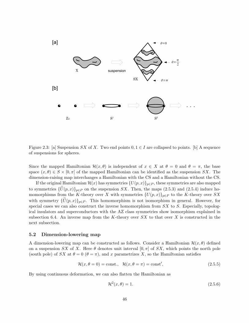
Figure 2.3: [a] Suspension SX of X. Two end points 0, 1 ∈ I are collapsed to points. [b] A sequenceof suspensions for spheres.
Since the mapped Hamiltonian H(x, θ) is independent of x ∈ X at θ = 0 and θ = π, the basespace (x, θ) ∈ S × [0, π] of the mapped Hamiltonian can be identified as the suspension SX. Thedimension-raising map interchanges a Hamiltonian with the CS and a Hamiltonian without the CS.
If the original HamiltonianH(x) has symmetries U(p, x)p∈P , these symmetries are also mapped
to symmetries U(p, x)p∈P on the suspension SX. Then, the maps (2.5.3) and (2.5.4) induce ho-momorphisms from the K-theory over X with symmetries U(p, x)p∈P to the K-theory over SX
with symmetry U(p, x)p∈P . This homomorphism is not isomorphism in general. However, forspecial cases we can also construct the inverse homomorphism from SX to S. Especially, topolog-ical insulators and superconductors with the AZ class symmetries show isomorphism explained insubsection 6.4. An inverse map from the K-theory over SX to that over X is constructed in thenext subsection.
5.2 Dimension-lowering map
A dimension-lowering map can be constructed as follows. Consider a Hamiltonian H(x, θ) definedon a suspension SX of X. Here θ denotes unit interval [0, π] of SX, which points the north pole(south pole) of SX at θ = 0 (θ = π), and x parametrizes X, so the Hamiltonian satisfies
H(x, θ = 0) = const., H(x, θ = π) = const′, (2.5.5)
By using continuous deformation, we can also flatten the Hamiltonian as
H2(x, θ) = 1. (2.5.6)
46

The above parametrization (x, θ) provides a natural dimensional reduction SX → X by fixing θ,say θ = π/2. This procedure, however, does not ensure providing the inverse map of Eqs.(2.5.3)and (2.5.4), because the flattened Hamiltonian does not have the form of the right hand side ofEqs.(2.5.3) or (2.5.4) in general.
To fix the form of the flattened Hamiltonian, following Teo and Kane [11], we introduce anartificial “action” S[H] of the Hamiltonian,
S[H] =
∫dxdθ Tr[∂θH∂θH]. (2.5.7)
By continuous deformation of the Hamiltonian, the value of action can reduce to reach its minimalvalue, whereH satisfies the saddle point equation with the constraint of H2 = 1, i.e. ∂2θH+H = 0. 11
Imposing the boundary condition (2.5.5), we can fix the form of the Hamiltonian as the saddle pointsolution,
H(x, θ) = sin θH1(x) + cos θH2, (2.5.8)
where the flatness condition H2(x, θ) = 1 implies
H21(x) = 1, H2
2 = 1, H1(x),H2 = 0. (2.5.9)
Then, by fixing θ = π/2, we have a dimensional reduction from H(x, θ) to H1(x).The last relation of Eq.(2.5.9) means that H2 act as CS on H1(x). Therefore, if the original
Hamiltonian H(x) does not support CS, Eq.(2.5.8) defines a dimensional reduction from non-chiralto chiral Hamiltonians. On the other hand, if the original Hamiltonian has CS Γ, then H1(x) hosts acouple of CSs, Γ and H2, with Γ, H2 = 0. Hence, H1(x) has redundancy due to the commutationrelation [H1(x),ΓH2] = 0. In the basis where Γ = 1 ⊗ σx and H2 = 1 ⊗ σy, the redundancy ofH1(x) is resolved as H1(x) = H3(x)⊗ σz, and thus we obtain
H(x, θ) = sin θH3(x)⊗ σz + cos θ1⊗ σy (2.5.10)
In this manner, a chiral Hamiltonian H(x, θ) is mapped to a non-chiral one H3(x).
6 Defect Hamiltonians and dimensional hierarchy of AZ classes
As explained in Sec. 5, topologically protected defect gapless states are classified by an adiabaticHamiltonian
H(k, r). (2.6.1)
Here the base space of the Hamiltonian is composed of momentum k, defined in the d-dimensionalBrillouin zone T d, and real-space coordinates r of a D-dimensional sphere SD surrounding a defect.For instance, the Hamiltonian of a point defect in 3-dimensions is given byH(kx, ky, kz, r1, r2), where(r1, r2) are the coordinates of a 2-dimensional sphere S2 surrounding the point defect. Anotherexample is a line defect in 3-dimensions, in which the Hamiltonian is H(kx, ky, kz, r1) where r1 isa parameter of a circle S1 enclosing the line defect. The case of D = 0 corresponds to a uniformsystem.
11 This procedure is known as the Morse theory. [89]
47

As mentioned above, the exact base space is T d × SD, but instead we consider a simpler spaceSd+D in the following. This simplification does not affect on “strong” topological nature of thesystem. Although the difference of the base space may result in “weak” topological indices of thesystem, they can be obtained as“strong” topological indices in lower dimensions, as will be arguedin section 6 in Chap. 3. Therefore, generality is not lost by the simplification.
6.1 Altland-Zirnbauer Symmetry Classes
The AZ symmetries, TRS, PHS, and CS, imply
TH(k, r)T−1 = H(−k, r),
CH(k, r)C−1 = −H(−k, r),
ΓH(k, r)Γ−1 = −H(k, r), (2.6.2)
respectively, where T and C are anti-unitary operators and Γ is a unitary operator.Below, we choose a convention that T and C commutes with each other, i.e. [T,C] = 0: Because
Eq.(2.6.2) yields [TCT−1C−1,H(k, r)] = 0 for any Hamiltonians with TRS and PHS, the unitaryoperator TCT−1C−1 should be proportional to the identity, TCT−1C−1 = eiβ1. The phase β canbe removed by a re-definition of the relative phase between T and C without changing the sign ofT 2 and C2, which leads to [T,C] = 0.
We denote the K-group over Sd+D with the AZ symmetries (2.6.2) by
KC(s, d,D) (s = 0, 1 mod 2) (2.6.3)
for complex AZ classes and
KR(s, d,D) (s = 0, . . . 7 mod 8) (2.6.4)
for real AZ classes. 12 Here s represents the AZ classes.
6.2 Dimension-raising map for defect Hamiltonians
Here we introduce a map from a Hamiltonian on a (d + D)-dimensional sphere (k, r) ∈ Sd+D toa Hamiltonian on Sd+D+1 by suspension (2.5.3) and (2.5.4). If the original Hamiltonian H(k, r)supports CS Γ, then the map is
Hnc(k, r, θ) = sin θHc(k, r) + cos θΓ, θ ∈ [0, π] , (2.6.5)
and if not, it is
Hc(k, r, θ) = sin θHnc(k, r)⊗ σz + cos θ1⊗ σy, θ ∈ [0, π] .
ΓH(k) = 0, Γ = σx.(2.6.6)
The dimension-raising map interchanges a Hamiltonian with CS and a Hamiltonian without CS.
12 Strictly speaking, the K-groups (2.6.3) and (2.6.4) are the reduced K-theory introduced in (2.3.17) which omitsobvious 0-dimensional K-group.
48

6.3 Dimension-lowering map for defect Hamiltonians
A dimension-lowering map Sd+D+1 → Sd+D can be constructed by the way in subsection 5.2:
H(k, r, θ) = sin θH1(k, r) + cos θH2, (2.6.7)
with
H21(k, r) = 1, H2
2 = 1, H1(k, r),H2 = 0. (2.6.8)
Then, by fixing θ = π/2, we have a dimensional reduction from H(k, r, θ) to H1(k, r)If the original Hamiltonian H(k, r) does not support CS, Eq.(2.6.7) defines a dimensional re-
duction from non-chiral to chiral Hamiltonians. If the original Hamiltonian has CS Γ = 1⊗ σx, weobtain
H(k, r, θ) = sin θH3(k, r)⊗ τz + cos θ1⊗ τy, (2.6.9)
and a chiral Hamiltonian H(k, r, θ) is mapped to a non-chiral one H3(k, r).
6.4 Dimensional hierarchy of AZ classes
In this section, we review the topological classification for AZ symmetry classes.[4, 5, 11] We providethe periodic table for the topological insulator and superconductor by using the K-group isomorphicmap between different dimensions and symmetries. Following Teo and Kane [11], we argue thedimensional hierarchy of the K-groups,
KC(s, d,D) = KC(s+ 1, d+ 1, D) = KC(s+ 1, d,D + 1) (2.6.10)
for complex AZ classes and
KR(s, d,D) = KR(s+ 1, d+ 1, D) = KR(s− 1, d,D + 1) (2.6.11)
for real AZ classes. We prove (2.6.10) and (2.6.11) below. For topological insulators and supercon-ductors in ten AZ symmetry classes, the following relations summarize their classification [5, 6, 11]
KC(s; d,D) = KC(s− d+D; 0, 0) = π0(Cs−d+D), (s = 0, 1 (mod 2)) (2.6.12)
KR(s; d,D) = KR(s− d+D; 0, 0) = π0(Rs−d+D), (s = 0, 1, · · · , 7 (mod 8)) (2.6.13)
where Cs (Rs) is the classifying space of s complex (real) AZ class in Table 2.2. The case of D = 0corresponds to the bulk topological classification, and the presence of topological defects shifts thedimension of the system. (2.6.12) and (2.6.13) provide the periodic table of topological insulatorsand superconductors (Tab. 2.4). [4, 5, 6, 11]
6.4.1 Complex AZ classes
The complex AZ classes consist of two symmetry class, class A for Hamiltonians with no symmetryand class AIII for those with the presence of CS. The symmetry classes are labeled by s = 0, 1 (mod2) as in Table 2.2. For the complex AZ classes, because of the absence of antiunitary symmetry,momentum k and coordinates r are not distinguished from each other, and thus KC(s, d,D) =KC(s, d+D, 0).
49

The dimensional raising maps, Eqs. (2.6.5) and (2.6.6), interchange Hamiltonians with CS andthose without CS, and thus they define a K-group homomorphismKC(s, d+D, 0) 7→ KC(s+1, d+D+1, 0), where s is also shifted by 1. At the same time, the dimensional lowering maps, Eqs. (2.6.7) and(2.6.9) define the inverse of the K-group homomorphism, i.e. KC(s+1; d+D+1, 0) 7→ KC(s; d+D, 0).Consequently, we obtain the K-group isomorphism Eq.(2.6.10).
6.4.2 Real AZ classes
The real AZ classes consist of eight symmetry classes which specified by the presence of TRS and/orPHS. The eight symmetry classes are labeled by s = 0, . . . , 7 (mod 8) as shown in Table 2.2. In thispaper, we take a convention that T and C commute with each other: [T,C] = 0. In this rule, thechiral operator Γ (that is a Hermitian matrix) is given by
Γ =
TC (s = 1, 5)iTC (s = 3, 7)
, (2.6.14)
where the following relation holds,
TΓT−1 = CΓC−1 =
Γ (s = 1, 5)−Γ (s = 3, 7)
. (2.6.15)
For real AZ classes hosting CS (s = 1, 3, 5, 7), one can raise the dimension of the base space byusing Eq.(2.6.5). The mapped Hamiltonian H(k, r, θ) supports either TRS or PHS, but does nothave both. The remaining symmetry depends on the type of θ one considers: If one increases thedimension d of the momentum space, the parameter θ should transform as θ → π − θ under TRSand PHS. In contrast, if one raises the dimension D of the position space, θ does not transformunder these symmetries. We call the former θ as k-type, and the latter as r-type. The differencein the transformation law of θ results in the difference of the remaining symmetry. For instance,consider the BDI class (s = 1) and k-type θ. In this case, because of Eq.(2.6.15), one finds thatthe mapped Hamiltonian, H(k, r, θ) = sin θH(k, r) + cos θ(TC), supports PHS. For real AZ classeswithout CS (s = 0, 2, 4, 6), the dimensional raising map is provided by Eq.(2.6.6). The mappedHamiltonian H(k, r, θ) has the CS, 1 ⊗ σx,H(k, r, θ) = 0. It also realizes TRS or PHS of theoriginal Hamiltonian H(k, r), in the form of T ⊗ σa or C ⊗ σa, where the choice of σa (a = 0, z)depends on the type of θ. The mapped Hamiltonian also has the rest of AZ symmetries, which isobtained by combination of these symmetries.
We summarize the AZ symmetries of the mapped Hamiltonian for each real AZ class in thelower part of Table 2.3. From this table, one finds that the dimensional raising maps, Eqs. (2.6.5)and (2.6.6), shift the label s of AZ classes by ±1, and thus they define K-group homomorphic maps,KR(s, d,D) 7→ KR(s+ 1, d+ 1, D) and KR(s, d,D) 7→ KR(s− 1, d,D + 1).
In a manner similar to complex AZ classes, the dimensional lowering maps, Eqs. (2.6.7) and(2.6.9), define the inverse of the K-group homomorphism, KR(s + 1, d + 1, D) 7→ KR(s, d,D) andKR(s − 1, d,D + 1) 7→ KR(s, d,D): Here note that Eqs. (2.6.7) and (2.6.9) determine uniquelyhow TRS and/or PHS of higher dimensional Hamiltonians act on the lower dimensional ones. As aresult, we have the K-group isomorphism, Eq.(2.6.11).
50

Table 2.3: Isomorphism from KR(s, d,D) to KF(s+1, d+1, D) and KF(s−1, d,D+1), (F = C,R).
AZ class Hamiltonian mapping Type of θ Mapped AZ class TRS PHS Chiral
A sin θH(k, r)⊗ σz + cos θ1⊗ σy k/r AIII 1⊗ σx
AIII sin θH(k, r) + cos θΓ k/r A
AI/AII sin θH(k, r)⊗ σz + cos θ1⊗ σyk BDI/CII T ⊗ σ0 T ⊗ σx 1⊗ σx
r CI/DIII T ⊗ σz T ⊗ σy 1⊗ σx
BDI/CII sin θH(k, r) + cos θ(TC)k D/C C
r AI/AII T
D/C sin θH(k, r)⊗ σz + cos θ1⊗ σyk DIII/CI C ⊗ σy C ⊗ σz 1⊗ σx
r BDI/CII C ⊗ σx C ⊗ σ0 1⊗ σx
DIII/CI sin θH(k, r) + cos θ(iTC)k AII/AI T
r D/C C
7 Topological invariants
In this section, we summarize the notation and the definition of topological invariants used in thisthesis.
7.1 Topological invariants in zero-dimension
Here, we introduce topological invariants in zero dimension. A Hamiltonian H in zero dimension ismerely a constant matrix, so adding extra trivial bands to the Hamiltonian makes any change of theHamiltonian possible. This means that no well-defined topological number of a single Hamiltonianis possible in the meaning of the stable-equivalence. We need a couple of Hamiltonians (H+,H−) todefine a topological number. We say that two coupled Hamiltonians, (H1+,H1−) and (H2+,H2−),are stable equivalent if they are continuously deformed into each other by adding the same extrabands to the coupled Hamiltonian. In other words, the stable equivalence implies (H+,H−) ∼(H+ ⊕Hext,H− ⊕Hext) with an extra band Hext.
7.1.1 Z (2Z) invariant
First, consider non particle-hole symmetric Hamiltonians. We assume here that H+ and H− havethe same matrix dimension. Denoting the numbers of empty (occupied) states of H± by n± (m±),the topological nature of the coupled Hamiltonians can be characterized by n+ −m+ and n− −m−since there appears a band crossing the Fermi level when these numbers are changed. Adding trivialp empty bands and q occupied ones to the coupled Hamiltonian, we also have the stable equivalence
51

Table 2.4: Topological periodic table for topological insulators and superconductors.[4, 5, 11] Thesuperscripts on Z and Z2 specify the integral representation of the corresponding topological indices.Z(Ch) and Z(W) are given by the Chern number Eq.(2.7.7) and the winding number Eq.(2.7.12),
respectively. Z(CS)2 and Z(CST)
2 represent the Chern-Simons integral Eq.(2.7.18) without and with the
time-reversal constraint Eq.(2.7.22), respectively. Z(FK)2 denotes the Fu-Kane invariant Eq.(2.7.21).
The Z2 invariants without any superscript are not expressed by these integrals, but they can bedefined operationally by the dimensional reduction or the Moore-Balents argument.
AZ class TRS PHS CS Cs or Rs δ = 0 δ = 1 δ = 2 δ = 3 δ = 4 δ = 5 δ = 6 δ = 7
A 0 0 0 C0 Z(Ch) 0 Z(Ch) 0 Z(Ch) 0 Z(Ch) 0
AIII 0 0 1 C1 0 Z(W) 0 Z(W) 0 Z(W) 0 Z(W)
AI 1 0 0 R0 Z(Ch) 0 0 0 2Z(Ch) 0 Z(FK)2 Z(CS)
2
BDI 1 1 1 R1 Z2 Z(W) 0 0 0 2Z(W) 0 Z2
D 0 1 0 R2 Z2 Z(CS)2 Z(Ch) 0 0 0 2Z(Ch) 0
DIII −1 1 1 R3 0 Z(CST)2 Z(FK)
2 Z(W) 0 0 0 2Z(W)
AII −1 0 0 R4 2Z(Ch) 0 Z(FK)2 Z(CS)
2 Z(Ch) 0 0 0
CII −1 −1 1 R5 0 2Z(W) 0 Z2 Z2 Z(W) 0 0
C 0 −1 0 R6 0 0 2Z(Ch) 0 Z2 Z(CS)2 Z(Ch) 0
CI 1 −1 1 R7 0 0 0 2Z(W) 0 Z(CST)2 Z(FK)
2 Z(W)
between these numbers,
(n+ −m+, n− −m−) ∼ (n+ −m+ + p− q, n− −m− + p− q). (2.7.1)
Therefore, the topological number in zero dimension is defined as
Ch0 :=n+ −m+ − n− +m−
2, (2.7.2)
because it should be invariant under the stable equivalence. Whereas Ch0 can take any integerfor class A and AI Hamiltonians, it takes only an even integer for class AII due to the Kramersdegeneracy of the spectrum.
7.1.2 Z2 invariant
For Hamiltonians with PHS satisfying C2 = 1, the following Z2 invariant can be introduced
ν0 = sgn [Pf(H+τx)] sgn [Pf(H−τx)] , (2.7.3)
with C = τxK: First, PHS implies H±τx = −(H±τx)T , which enables us to define the Pfaffian of
H±τx. Then, from the relation
[Pf(H±τx)]∗ = Pf(H∗
±τx) = Pf(τTx (H±τx)T τx) = Pf(H±τx) (2.7.4)
52

the sign of Pf(H±τx) is quantized as ±1. Taking into account the stable equivalence, we find thateach of Pf(H±τx) does not give a Z2 invariant, but their product ν0 defines it.
In AZ classes, BDI and D in zero dimension support this Z2 invariant. Class DIII also has PHSwith C2 = 1, but ν0 becomes trivial in this case because of the Kramers degeneracy.
7.2 Chern number and winding number
Here we summarize the analytic expressions of integer Z topological invariants, i.e. the Chernnumbers in even-dimensions, and the winding numbers in odd-dimensions.
7.2.1 Q-function
It is useful to introduce the so called “Q-function”[4] defined by
Q(k, r) =∑
Eα(k,r)>EF
|uα(k, r)⟩ ⟨uα(k, r)| −∑
Eα(k,r)<EF
|uα(k, r)⟩ ⟨uα(k, r)| , (2.7.5)
where |uα(k, r)⟩ is an eigenstate ofH(k, r) with an eigen energy Eα(k, r). The Q-function is nothingbut the flattened Hamiltonian of H(k), and it has the following properties:
Q2(k, r) = 1, Q(k, r) |uα(k, r)⟩ =
|uα(k, r)⟩ , (Eα(k, r) > EF)− |uα(k, r)⟩ , (Eα(k, r) < EF)
. (2.7.6)
The symmetry of the Q-function is the same as the original Hamiltonian H(k, r).
7.2.2 Chern number
In the 2n-dimensional base space, the n-th Chern number Chn is defined by
Chn =1
n!
(i
2π
)n ∫trFn, (2.7.7)
with F = dA + A ∧ A. Here Aαβ = ⟨uα duβ⟩ is the connection of occupied states |uα(k, r)⟩ ofH(k, r), and the trace is taken for all occupied states. The Chern number is rewritten as
Chn = − 1
22n+1
1
n!
(i
2π
)n ∫trQ(dQ)2n. (2.7.8)
It is also useful to express the Chern number in terms of the Green function,[90] G(ω,k, r) =[iω −H(k, r)]−1, when we discuss the electromagnetic and/or heat responses. The Chern numberis recast into
Chn = − n!
(2πi)n+1 (2n+ 1)!
∫tr[GdG−1
]2n+1. (2.7.9)
Although the Chern number can be defined in any even dimensions, symmetry of the systemsometimes prohibits a non-zero Chern number. For example, consider an antiunitary symmetry
AH(k∥,k⊥)A−1 = H(k∥,−k⊥). (2.7.10)
53

Since the Q-function has the same symmetry, AQ(k∥,k⊥)A−1 = Q(k∥,−k⊥), we find
Chn = − 1
22n+1
1
n!
(i
2π
)n ∫tr[A−1Q(k∥,−k⊥)dQ(k∥,−k⊥)
2nA]
= − 1
22n+1
1
n!
(i
2π
)n ∫tr[Q∗(k∥,−k⊥)dQ
∗(k∥,−k⊥)2n]
= −(−1)2n−d∥
22n+1
1
n!
(i
2π
)n ∫tr[Q∗(k)dQ∗(k)2n
]= (−1)n−d∥Ch∗n.
= (−1)n−d∥Chn, (2.7.11)
where we have used the fact that Chn is an integer in the last line. The above equation yieldsChn = 0 if n = d∥ + 1 (mod 2).
7.2.3 Winding number
In the 2n+ 1-dimensional base space, the winding number is defined by,
N2n+1 =n!
2(2πi)n+1(2n+ 1)!
∫trΓ(H−1dH
)2n+1, (2.7.12)
if the Hamiltonian H(k, r) has CS, ΓH(k, r)Γ−1 = −H(k, r). Equivalently, the winding number(2.7.12) is expressed by the Q-function,
N2n+1 =(−1)nn!
2(2πi)n+1(2n+ 1)!
∫trΓQ (dQ)2n+1 . (2.7.13)
In the diagonal base of Γ = diag(1,−1), the Q-function is off-diagonal,
Q(k, r) =
(0 q(k, r)
q†(k, r) 0
), (2.7.14)
so the winding number N2n+1 is simplified as
N2n+1 =n!
(2πi)n+1(2n+ 1)!
∫tr[qdq†
]2n+1. (2.7.15)
In a manner similar to the Chern numbers, symmetry of the system sometimes prohibits anon-zero winding number. For example, the antiunitary symmetry in Eq.(2.7.10) leads
N2n+1 =(−1)nn!
2(2πi)n+1(2n+ 1)!
∫tr[ΓA−1Q(k∥,−k⊥)dQ(k∥,−k⊥)
2n+1A]
=ηΓ(−1)nn!
2(2πi)n+1(2n+ 1)!
∫tr[ΓQ∗(k∥,−k⊥)dQ
∗(k∥,−k⊥)2n+1
]=
ηΓ(−1)2n+1−d∥(−1)nn!
2(2πi)n+1(2n+ 1)!
∫tr[ΓQ∗(k)dQ∗(k)2n+1
]= (−1)n−d∥ηΓN
∗2n+1
= (−1)n−d∥ηΓN2n+1, (2.7.16)
where ηΓ = ± specifies the commutation(+) or anti-commutation(-) relation between Γ and A.Hence, N2n+1 = 0 when n = d∥ + (ηΓ − 1)/2 (mod 2).
54

7.2.4 2Z topological invariant
In the real AZ classes, there are two integer K-groups, KR(s; d,D) = Z for s = d − D (mod 8)and KR(s; d,D) = 2Z for s = d−D + 4 (mod 8), where “2Z” means that the corresponding Chernnumber defined by Eq.(2.7.7) or the winding number defined by Eq.(2.7.12)) takes an even integer.Here, we outline the proof why the topological number becomes even when s = d−D + 4 (mod 8)and d ≥ 1.
Consider a Hamiltonian H(k, r) in real AZ class with s = d−D + 4 (mod 8). Choosing one ofthe momenta as the polar angle θ of the base space Sd+D and denoting the rest momenta by k′,AZ symmetries are expressed as TH(θ,k′, r)T−1 = H(π − θ,−k′, r), CH(θ,k′, r)C−1 = −H(π −θ,−k′, r), and ΓH(θ,k′, r)Γ−1 = −H(θ,k′, r). Thus, the Hamiltonian on the equator, H(θ =π/2,k′, r), retains all the AZ symmetries that the original Hamiltonian H(k, r) has. Furthermore,the equator Hamiltonian is found to be topologically trivial, since its K-group is given as KR(s; d−1, D) = KR(s− d+1+D; 0, 0) = π0(R5) = 0 when s = d−D+4 (mod 8). This means that we canpinch the (d+D)-dimensional sphere Sd+D on the equator by deforming the equator Hamiltonianinto a constant Hamiltonian without breaking the symmetries.
After the pinching, the north and south hemispheres turn into a couple of (d+D)-dimensionalspheres Sd+D, and the original Hamiltonian reduces to a couple of Hamiltonians in complex AZ classwith the same s = d−D+4 (mod 8). Since their K-groups obey KC(s; d,D) = KC(s−d+D; 0, 0) =π0(C4) = Z, the couple of Hamiltonian have definite integer topological numbers Nnorth and Nsouth,which are defined by Eq. (2.7.7) or Eq. (2.7.12). These topological numbers, however, are notindependent. Because TRS and/or PHS in the original Hamiltonian exchange the north and southhemispheres, Nnorth and Nsouth must be the same. Consequently, the topological number of theoriginal Hamiltonian, which is given by the sum of Nnorth and Nsouth, must be even,
7.3 Z2 topological invariant
In this appendix we summarize various arguments and formulas to define Z2 invariants. i.e. thedimensional reduction,[13, 6] the Moore-Balents argument, [91] and the integral formulas.
7.3.1 Dimensional reduction
In our topological periodic tables, a sequence of Z2 indices follows a Z index as the dimension ofthe system decreases. This structure makes it possible to define the corresponding Z2 invariants bydimensional reduction:[13, 6] Let us consider a (d+2)-dimensional Hamiltonian H(k, kd+1, kd+2, r)that is characterized by the Z index mentioned in the above. Then, we can construct maps fromthis Hamiltonian to one and two lower dimensional Hamiltonians, by considering H(k, kd+1, 0, r)and H(k, 0, 0, r), respectively. These maps define surjective homomorphic maps from Z to Z2. Asa result, the first and second descendant Z2 invariants , ν1st and ν2nd, of the lower dimensionalHamiltonians are obtained as
(−1)ν1st = (−1)ν2nd = (−1)N , (2.7.17)
where N is the integer topological invariant ofH(k, kd+1, kd+2, r). N is the Chern number Eq.(2.7.7)for non-chiral class or the winding number Eq. (2.7.12) for chiral class.
55

7.3.2 Moore-Balents argument for second descendant Z2 index
For the second descendant Z2 index (d = s + D − 2) of Table 2.4 with d ≥ 1, there is anotheroperational definition of the Z2 invariant, which was first discussed by Moore and Balents.[91]Consider a Hamiltonian H(k, r) in real AZ class with d = s+D− 2. Choosing one of the momentaas the polar angle θ of the base sphere Sd+D and denoting the rest by k′, the AZ symmetriesare expressed as TH(θ,k′, r)T−1 = H(π − θ,−k′, r), CH(θ,k′, r)C−1 = −H(π − θ,−k′, r), andΓH(θ,k′, r)Γ−1 = −H(θ,k′, r). Then, take only the north hemisphere (0 ≤ θ ≤ π/2) of the system.Although TRS and/or PHS cannot be retained only on the north hemisphere, they are retained at itsboundary, i.e. the equator. Indeed the Hamiltonian on the equator H(θ = π/2,k′, r) has the samesymmetry of the original HamiltonianH(k, r), and thus its K-group isKR(s; d−1, D) = π0(R3) = 0.
To define the topological number, we introduce another hemisphere in the following man-ner. As mentioned in the above, the K-group of the equator Hamiltonian is trivial. There-fore the equator Hamiltonian can smoothly shrink into a point H0 with keeping the AZ sym-metry of the (d − 1)-dimensional momentum space. This deformation defines a HamiltonianH(θ,k′, r) on a new hemisphere, say, a new south hemisphere, where the new Hamiltonian in-terpolates H(θ = π/2,k′, r) at the equator (θ = π/2) to H0 at the south pole (θ = π). Notehere that θ of H(θ,k′, r) is just an interpolating parameter, and thus it transforms trivially un-der the AZ symmetries as T H(θ,k′, r)T−1 = H(θ,−k′, r), CH(θ,k′, r)C−1 = −H(θ,−k′, r), andΓH(θ,k′, r)Γ−1 = −H(θ,k′, r).
Now define the topological number. Sewing the new south and the original north hemispherestogether, we have a Hamiltonian on a sphere. In contrast to the original Hamiltonian, the resultantHamiltonian no longer has TRS and/or PHS since θ transforms differently in the north hemisphereand the south hemisphere. It belongs to a complex AZ class (A or AIII), so it can host a nonzerointeger topological number N given by the Chern number Ch(d+D)/2 or the winding number Nd+D.
Its value, however, depends on the choice of the interpolating Hamiltonian H(θ,k′, r) in general.Therefore, N itself does not characterize the topological nature of the original Hamiltonian. Never-theless, its parity (−1)N is uniquely determined: Take another interpolating Hamiltonian H′(θ,k′, r)which may give a different integer N ′. The difference between N and N ′ can be evaluated as thetopological number of the Hamiltonian that is obtained by sewing the hemispheres of H(θ,k′, r)and H′(θ,k′, r) together. In this case, the combined Hamiltonian keeps TRS and/or PHS whichare the same as those of the original Hamiltonian except the r-type transformation of θ. Therefore,its K-group is KR(s, d − 1, D + 1) = π0(R4) = 2Z, which implies that N −N ′ must be even. As aresult, the parity (−1)N is unique, i.e. (−1)N = (−1)N
′. The parity defines the Z2 invariant of the
original Hamiltonian.
7.3.3 Chern-Simons invariant for first descendant Z2 index in odd-dimensional non-chiral real class
The integral representation of the first descendant Z2 invariant in non-chiral real class is given bythe Chern-Simons form. [13] Consider a Hamiltonian H(k, r) on the base space Sd+D with oddd+D. The Z2 topological invariant is given by
ν =2
((d+D + 1)/2)!
(i
2π
)(d+D+1)/2 ∫Sd+D
CSd+D (mod 2). (2.7.18)
56

Here CSd+D is the Chern-Simons (d+D)-form given by [92]
CS2n+1 = (n+ 1)
∫ 1
0dttr
(A(tdA+ t2A2)n
)(2.7.19)
where Aαβ(k, r) = ⟨uα(k, r) duβ(k, r)⟩ is the connection defined by occupied states |uα(k, r)⟩.Some of lower dimensional Chern-Simons forms are
CS1 = trA,
CS3 = tr
(AdA+
2
3A3
),
CS5 = tr
(A(dA)2 +
3
2A3dA+
3
5A5
).
(2.7.20)
Here phases of the occupied states should be globally defined on the overall parameter manifoldSd+D so as the connection A is non-singular. The Z2 nontriviality of this integral is ensured by thedimensional reduction discussed in Sec.7.3.1.
The Chern-Simons invariant characterizes the real AZ classes with (s, δ) = (2n, 2n− 1) (mod 8)in Table 2.4.
7.3.4 Fu-Kane invariant for first and second descendant Z2 indices in even-dimensionalTRS class
In the presence of TRS, the Z2 invariant can be introduced as [93]
ν =1
((d+D)/2)!
(i
2π
)(d+D)/2[∫
Sd+D1/2
trF (d+D)/2 −∮∂Sd+D
1/2
CSd+D−1
](mod 2), (2.7.21)
where Sd+D1/2 is a (north) hemisphere of Sd+D and ∂Sd+D
1/2∼= Sd+D−1 is the equator. We suppose here
that the north hemisphere and the south one are exchanged by TRS, but the equator is invariant.The valence band wave functions of the Chern-Simons form in Eq.(2.7.21) must be smoothly definedon the equator ∂Sd+D
1/2 (not on the hemisphere Sd+D1/2 ). An appropriate gauge condition is needed to
obtain the Z2 nontriviality, and thus we impose the time-reversal constraint for the valence bandBloch wave functions |un(k, r)⟩ as [93]
wmn(k, r) = ⟨um(−k, r) Tun(k, r)⟩ ≡ const. (2.7.22)
on the equator (k, r) ∈ ∂Sd+D1/2 . The Z2 invariant Eq.(2.7.21) picks up an obstruction to choosing
the gauge satisfying (2.7.22) on overall Brillouin zone.In Table 2.4, the Fu-Kane invariant characterizes the real AZ classes with (s, δ) = (4n+3, 4n+2)
(mod 8) and those with (s, δ) = (4n + 4, 4n + 2) (mod 8). Note that the Fu-Kane invariant is notapplicable to class BDI and CII, since the presence of CS that commutes with TRS makes theintegral Eq.(2.7.21) trivial.
7.3.5 Constrained Chern-Simons invariant for second descendant Z2 index in odd-dimensional chiral TRS class
Consider a Hamiltonian H(k, r) on the base space Sd+D with odd d +D. If the Hamiltonian hasCS and TRS that anti-commute with each other, then the Z2 invariant of the Hamiltonian can be
57

given in a form of the Chern-Simons integral: To see this, first consider the dimension raising mapin Eq.(2.6.5),
H(k, r, θ) = sin θH(k, r) + cos θΓ. (2.7.23)
Since the mapped Hamiltonian on Sd+D+1 has TRS and is even-dimensional, we can define theFu-Kane Z2 invariant of H(θ,k, r) as
ν =1
((d+D + 1)/2)!
(i
2π
)(d+D+1)/2[∫
Sd+D+11/2
trF (d+D+1)/2 −∮∂Sd+D+1
1/2
CSd+D
](mod 2).
(2.7.24)
It is convenient to choose a k-type θ and take the equator as θ = π/2. Then, we can show that thefirst term of Eq.(2.7.24) is identically zero due to TRS and CS of H(k, r).[11] Also the equator isnothing but the original base space Sd+D, Eq.(2.7.24) is recast into
ν =1
((d+D + 1)/2)!
(i
2π
)(d+D+1)/2 ∫Sd+D
CSd+D (mod 2), (2.7.25)
with the time-reversal constraint Eq.(2.7.22) on (k, r) ∈ Sd+D.[11] Note here that Eq.(2.7.25) isa half of Eq.(2.7.18) so the additional gauge constraint Eq.(2.7.22) is necessary to obtain the Z2
nontriviality.The constrained Chern-Simons invariant characterizes the real AZ classes with (s, δ) = (4n +
3, 4n+ 1) (mod 8) in Table 2.4.
58

Chapter 3
Topological phases with order-twopoint group symmetry
In this chapter, we provide the complete classification of topological crystalline insulators and su-perconductors with an additional order-two point group symmetry. The symmetry we consideris general, and it includes global Z2 symmetry, reflection, two-fold rotation, inversion, and theirmagnetic point group symmetries. In the cases of the order-two symmetries, the topological classi-fication is replaced by the extension problem of the Clifford algebras. The topological classificationindicates that topological defect gapless states can be considered as boundary gapless states in lowerdimensional systems. The resultant topological periodic table shows a novel periodicity in the num-ber of the flipped coordinates under the order-two additional spatial symmetry, in addition to theBott-periodicity in the space dimensions. Using the new topological periodic table, various symme-try protected topological gapless modes at topological defects are identified in a unified manner. Inaddition, we also present a topological classification of Fermi points (for example, Weyl semimetalsand superconductors, and Dirac semimetals) in the crystalline insulators and superconductors. Thebulk topological classification and the Fermi point classification show the bulk-boundary correspon-dence in terms of the K-theory.
The organization of this chapter is as follows. In Sec. 1, we introduce the order-two point groupsymmetries and their representations of defect Hamiltonians. Our main results are summarized inSec. 2. We show relations between K-groups with different order-two additional spatial symmetriesand dimensions. The derivation and proof are given in Sec. 3. The classifying spaces of AZ classeswith additional order-two symmetry are summarized in Sec. 4. In Sec. 5, we discuss properties ofthe obtained K-groups in the presence of additional symmetry. A novel periodicity in the num-ber of flipped coordinates under the additional symmetry is pointed out. We also find that theK-groups naturally implement topological defects as boundaries of lower dimensional crystallineinsulators/superconductors. Crystalline weak topological indices are argued in Sec. 6. We alsoapply our formalism to a classification of Fermi point protected by additional order-two symmetryin Sec. 7. By combing the results in Secs. 2 and 7, the bulk-boundary correspondence of K-groupsare presented. We conclude the present chapter with some discussions in Sec. 8.
59

1 Order-two point group symmetries
In addition to the Altland-Zirnbauer (AZ) symmetries, i.e. time-reversal symmetry (TRS), particle-hole symmetry (PHS), and chiral symmetry (CS), we assume an additional symmetry of Hamiltoni-ans. As an additional symmetry, we consider general order-two (magnetic) point group symmetry.Order-two point group symmetry S implies that the symmetry operation in twice trivially acts onspatial coordinate,
S : (x∥,x⊥) 7→ (−x∥,x⊥) (3.1.1)
with x∥ = (x1, x2, · · · , xd∥) and x⊥ = (xd∥+1, xd∥+2 · · · , xd). The order-two point group symmetryincludes reflection, two-fold spatial rotation and inversion. It also permits global Z2 symmetrysuch as a two-fold spin rotation. The anti-unitary case admits order-two magnetic point groupsymmetries. Under an order-two spatial symmetry, the momentum k in the base space of theHamiltonian transforms as
k →
(−k∥,k⊥), for S = U
(k∥,−k⊥), for S = A, (3.1.2)
with k∥ = (k1, k2, · · · , kd∥) and k⊥ = (kd∥+1, kd∥+2 · · · , kd). Here S can be either unitary U oranti-unitary A. Note that like time-reversal operator, the anti-linearity of A results in the minussign of the transformation law of k.
In contrast to non-spatial AZ symmetries, the spatial coordinate r of the D-dimensional spheresurrounding a topological defect also transforms non-trivially under order-two spatial symmetry. Todetermine the transformation law, we specify the coordinate r of the D-dimensional sphere. First,to keep the additional symmetry, the topological defect should be invariant under S. Therefore, theadditional symmetry S maps the D-dimensional sphere (with a radius a > 0) given by
n2 = a2, n = (n1, n2, · · · , nD+1), (3.1.3)
into itself, inducing the transformation
n → (−n∥,n⊥), (3.1.4)
with n∥ = (n1, n2, · · · , nD∥) and n⊥ = (nD∥+1, nD∥+2 · · · , nD+1). When D∥ ≤ D, we can introducethe coordinate r of the D-dimensional sphere by the stereographic projection of n as shown in Fig.3.1,
ri =ni
a− nD+1, (i = 1, · · ·D), (3.1.5)
which gives a simple transformation law of r as
r → (−r∥, r⊥), (3.1.6)
with r∥ = (r1, r2, · · · , rD∥) and r⊥ = (rD∥+1, rD∥+2 · · · , rD). Below, we assume D∥ ≤ D, sincethe bulk-boundary correspondence for topological defects works only in this case. The assumptionD∥ ≤ D implies that there is at least one unchanged coordinate, i.e. xD+1, against the order-twopoint group transformation.
60

Figure 3.1: A stereographic projection of the sphere SD.
Now the order-two unitary symmetry is expressed as
UH(k, r)U−1 = H(−k∥,k⊥,−r∥, r⊥), (3.1.7)
and the order-two anti-unitary symmetry is
AH(k, r)A−1 = H(k∥,−k⊥,−r∥, r⊥). (3.1.8)
Here H(k, r) is the defect Hamiltonian introduced in the previous chapter (eq. (2.6.1)). We supposethat
S2 = ϵS = ±1, (S = U or A), (3.1.9)
and S commutes or anticommutes with coexisting AZ symmetries,
ST = ηTTS, SC = ηCCS, SΓ = ηΓΓS. (3.1.10)
where ηT = ±1, ηC = ±1, and ηΓ = ±1. For a faithful representation of order-two symmetry,the sign ϵS of S2 must be 1, but a spinor representation of rotation makes it possible to obtainϵS = −1. For instance, two-fold spin rotation S = eiπsi/2 (i = 1, 2, 3) obeys S2 = −1. Note thatwhen S = U , we can set ϵS = 1 by multiplying S by the imaginary unit i, but this changes the(anti-)commutation relations with T and/or C at the same time.
Our classification framework also works even for order-two anti-symmetry S defined by
UH(k, r)U−1 = −H(−k∥,k⊥,−r∥, r⊥), (3.1.11)
AH(k, r)A−1 = −H(k∥,−k⊥,−r∥, r⊥), (3.1.12)
where S can be either unitary U or anti-unitary A. Such an anti-symmetry can be realized bycombining any of order-two symmetries with CS or PHS. In a similar manner as S, we define ϵ
S,
ηT , ηC and ηΓ by
(S)2 = ϵS, ST = ηTTS, SC = ηCCS, SΓ = ηΓΓS. (3.1.13)
The existence of an order-two spatial symmetry S gives additional constraints on the classifyingspace. In the subsequent sections, we provide the resulting K-group of the homotopy classification.
61

2 K-group in the presence of additional symmetry: additionalsymmetry class
In this section we present the results of topological classification of topological crystalline insulatorsand superconductors and their topological defects protected by an additional order-two point groupsymmetry. The derivation and proof are given in the appended paper (Ref. [38]). We briefly sketcha proof in the subsection 3.
The topological classification for order-two point group symmetries is divided into the threepieces:
(i) Complex AZ classes with additional order-two unitary symmetry
(ii) Complex AZ classes with additional order-two antiunitary symmetry
(iii) Real AZ classes with additional order-two symmetry
We give their topological classification classification below. We introduce a useful parameter t refer-eed to as “additional symmetry class” which is an analogy to AZ symmetry classes, and characterizestypes of additional symmetries.
2.1 Complex AZ classes with additional order-two unitary symmetry
The complex AZ classes consist of class A and class AIII. In class AIII Hamiltonians are imposed byCS, ΓH(k, r)Γ−1 = −H(k, r). Now we impose an additional order-two symmetry/antisymmetry,
UH(k, r)U−1 = H(−k∥,k⊥,−r∥, r⊥), (symmetry)
UH(k, r)U−1 = −H(−k∥,k⊥,−r∥, r⊥), (antisymmetry)(3.2.1)
on complex AZ classes. Since there is no anti-unitary symmetry, a phase factor of U and U do notchange the topological classification, and thus the sign of U2 and (U)2 can be fixed to be 1. Forclass AIII, we specify the commutation/anti-commutation relation between U and Γ (U and Γ) byUηΓ (UηΓ). Note that UηΓ in class AIII is essentially the same as UηΓ because they can be convertedto each other by the relation
UηΓ = ΓUηΓ . (3.2.2)
We denote the obtained K-group by
KUC (s, t; d, d∥, D,D∥). (3.2.3)
Here d (D) is the total space dimension (defect co-dimension), and d∥ (D∥) is the number of theflipping momenta (defect surrounding parameters) under the additional symmetry transformation,as was introduced in Sec.1. The label s = 0, 1 (mod 2) indicates the AZ class (s = 0 for class A ands = 1 for class AIII) to which the Hamiltonian belongs, and t = 0, 1 (mod 2) specifies the coexistingadditional unitary symmetry as in Table. 3.1.
We can prove the following relation: [38]
KUC (s, t; d, d∥, D,D∥) = KU
C (s− d+D, t− d∥ +D∥; 0, 0, 0, 0). (3.2.4)
62

Table 3.1: Possible types (t = 0, 1 (mod 2)) of order-two additional unitary symmetries in complexAZ class (s = 0, 1 (mod 2)). U and U represent symmetry and antisymmetry, respectively. Thesubscript of UηΓ and UηΓ specifies the relation ΓU = ηΓUΓ. Symmetries in the same parenthesisare equivalent because of Eq. (3.2.2).
s AZ class t = 0 t = 1
0 A U U
1 AIII (U+, U+) (U−, U−)
This relation implies that topological natures of the system can be deduced from those in 0-dimension. As we show in the section 4, the classifying spaces of the 0-dimensional K-group reduceto complex Clifford algebra, and we can obtain [68, 38]
KUC (s, t = 0; 0, 0, 0, 0) = π0(Cs × Cs) = π0(Cs)⊕ π0(Cs),
KUC (s, t = 1; 0, 0, 0, 0) = π0(Cs+1).
(3.2.5)
where Cs(s = 0, 1) represents the classifying space of complex AZ classes. (See Table 2.2.)
2.2 Complex AZ classes with additional order-two antiunitary symmetry
Next, we consider order-two anti-unitary symmetry A or A as an additional symmetry:AH(k, r)A−1 = H(k∥,−k⊥,−r∥, r⊥), (symmetry)
AH(k, r)A−1 = −H(k∥,−k⊥,−r∥, r⊥), (antisymmetry)(3.2.6)
As listed in Table 3.2, two different order-two anti-unitary symmetries A± and their correspondinganti-symmetries A± are possible in class A, depending on the sign of A2 or (A)2, i.e. (AϵA)2 = ϵA,(AϵA)2 = ϵA. In a similar manner, class AIII have two different types of additional anti-unitarysymmetries, AϵA
ηΓ(ϵA = ±1, ηA = ±1), and their corresponding anti-symmetries, AϵA
ηΓ(ϵA = ±1, ηA =
±1), where ϵA represents the sign of A2 or (A)2 and ηΓ indicates the commutation (ηΓ = 1) or theanti-commutation (ηΓ = −1) relation between A and Γ or those between A and Γ. Note that AϵA
ηΓ
and AϵAηΓηΓ are equivalent in class AIII since they can be related to each other as
AϵAηΓ
= ΓAϵAηΓηΓ
. (3.2.7)
The existence of the anti-unitary symmetry introduces real structures in complex AZ classes.Actually, in Eq. (3.2.6) by regarding (k⊥, r∥) as “momenta”, and (k∥, r⊥) as “spatial coordinates”, A
and A can be considered as usual TRS and PHS in AZ classes, respectively. From this identification,a system in complex AZ class with an additional anti-unitary symmetry can be mapped into a realAZ class, as summarized in Table 3.2. As a result, the K-group of Hamiltonians with the symmetrys (s = 0, 1, 2, . . . , 7 (mod 8)) of Table 3.2
KAC (s; d, d∥, D,D∥), (3.2.8)
reduces to the K-group of real AZ classes in Eq. (2.6.13), [38]
KAC (s; d, d∥, D,D∥) = KR(s; d− d∥ +D∥, D −D∥ + d∥). (3.2.9)
63

Table 3.2: Possible types (s = 0, 1, . . . , 7 (mod 8)) of order-two additional anti-unitary symmetriesin complex AZ class. A and A represent symmetry and anti-symmetry, respectively. The superscriptof AϵA and AϵA
ηΓrepresent the sign of the square A2 = ϵA, and the subscript of AϵA
ηΓspecifies the (anti-
)commutation relation ΓA = ηΓAΓ. Symmetries in the same parenthesis are equivalent because ofEq. (3.2.7).
s AZ class Coexisting symmetry Mapped AZ class
0 A A+ AI
1 AIII (A++, A
++) BDI
2 A A+ D
3 AIII (A−−,A
+−) DIII
4 A A− AII
5 AIII (A−+, A
−+) CII
6 A A− C
7 AIII (A+−, A
−−) CI
where d (D) is the total space dimension (defect co-dimension), and d∥ (D∥) is the number of theflipping momentum (defect surrounding parameter) under the additional symmetry transformation.From Eq. (2.6.13), we have
KAC (s; d, d∥, D,D∥) = KA
C (s− d+D + 2(d∥ −D∥); 0, 0, 0, 0), (3.2.10)
with
KAC (s; 0, 0, 0, 0) = π0(Rs). (3.2.11)
2.3 Real AZ classes with additional order-two symmetry
Hamiltonians in eight real AZ classes are invariant under TRS, TH(k, r)T−1 = H(−k, r), and/orPHS, CH(k, r)C−1 = −H(−k, r). In addition to TRS and/or PHS, we enforce one of order-twounitary/antiunitary spatial symmetries, U , U , A, and A on the Hamiltonians,
UH(k, r)U−1 = H(−k∥,k⊥,−r∥, r⊥), ( unitary symmetry )
UH(k, r)U−1 = −H(−k∥,k⊥,−r∥, r⊥), ( unitary antisymmetry )
AH(k, r)A−1 = H(k∥,−k⊥,−r∥, r⊥), ( antiunitary symmetry )
AH(k, r)A−1 = −H(k∥,−k⊥,−r∥, r⊥). ( antiunitary antisymmetry )
(3.2.12)
In class AI and AII, which support TRS, we have the following equivalence relations between theadditional symmetries,
U ϵUηT
= iU−ϵU−ηT
= TAηT ϵT ϵUηT = iTAηT ϵT ϵU
−ηT,
U ϵUηT
= iU−ϵU−ηT
= TAηT ϵT ϵUηT = iTAηT ϵT ϵU
−ηT,
(3.2.13)
where the superscript ϵS = ± of S (S = U,U,A,A) denotes the sign of S2, and the subscript ηT ofS specifies the commutation (ηT = +) or anti-commutation (ηT = −) relation between S and T . In
64

Table 3.3: Possible types (t = 0, 1, 2, 3 (mod 4)) of order-two additional symmetries in real AZ class(s = 0, 1, . . . , 7 (mod 8)). U and U represent unitary symmetry and anti-symmetry, respectively,and A and A represent anti-unitary symmetry and anti-symmetry, respectively. The superscript of S(S = U, U, A, A) indicates the sign of S2, and the subscript of S specifies the commutation(+)/anti-commutation(-) relation between S and TRS and/or PHS. For BDI, DIII, CII and CI, where bothTRS and PHS exist, S has two subscripts, in which the first one specifies the (anti-)commutationrelation between S and T and the second one specifies that between S and C. Symmetries in thesame parenthesis are equivalent because of Eqs. (3.2.13), (3.2.14) and (3.2.15).
s AZ class t = 0 t = 1 t = 2 t = 3
0 AI(U+
+ , U−− ) (U+
− , U−+ ) (U+
− , U−+ ) (U+
+ , U−− )
(A++, A
+−) (A−
+, A−−) (A−
−, A−+) (A+
+, A+−)
1 BDI(U+
++, U−−−, U
+++, U
−−−) (U+
+−, U−−+, U
+−+, U
−+−) (U+
−−, U−++, U
+−−, U
−++) (U+
−+, U−+−, U
++−, U
−−+)
(A+++, A
+−−, A
+++, A
+−−) (A+
+−, A+−+, A
−−+, A
−+−) (A−
−−, A−++, A
−−−, A
−++) (A−
−+, A−+−, A
++−, A
+−+)
2 D(U+
+ , U−− ) (U+
+ , U−− ) (U+
− , U−+ ) (U+
− , U−+ )
(A++, A
+−) (A+
+, A+−) (A−
−, A−+) (A−
+, A−−)
3 DIII(U+
++, U−−−, U
−++, U
+−−) (U+
−+, U−+−, U
+−+, U
−+−) (U+
−−, U−++, U
−−−, U
+++) (U+
+−, U−−+, U
++−, U
−−+)
(A−++, A
−−−, A
+++, A
+−−) (A+
−+, A++−, A
+−+, A
++−) (A+
−−, A+++, A
−−−, A
−++) (A−
+−, A−−+, A
−+−, A
−−+)
4 AII(U+
+ , U−− ) (U+
− , U−+ ) (U+
− , U−+ ) (U+
+ , U−− )
(A−+, A
−−) (A+
−, A++) (A+
−, A++) (A−
+, A−−)
5 CII(U+
++, U−−−, U
+++, U
−−−) (U+
+−, U−−+, U
+−+, U
−+−) (U+
−−, U−++, U
+−−, U
−++) (U+
−+, U−+−, U
++−, U
−−+)
(A−++, A
−−−, A
−++, A
−−−) (A−
+−, A−−+, A
+−+, A
++−) (A+
−−, A+++, A
+−−, A
+++) (A+
−+, A++−, A
−+−, A
−−+)
6 C(U+
+ , U−− ) (U+
+ , U−− ) (U+
− , U−+ ) (U+
− , U−+ )
(A−+, A
−−) (A−
+, A−−) (A+
−, A++) (A+
−, A++)
7 CI(U+
++, U−−−, U
−++, U
+−−) (U+
−+, U−+−, U
+−+, U
−+−) (U+
−−, U−++, U
−−−, U
+++) (U+
+−, U−−+, U
++−, U
−−+)
(A+++, A
+−−, A
−++, A
−−−) (A−
−+, A−+−, A
−−+, A
−+−) (A−
−−, A−++, A
+−−, A
+++) (A+
+−, A+−+, A
++−, A
+−+)
a similar manner, in class D and C, PHS leads to the following equivalence relationsU ϵUηC
= iU−ϵU−ηC
= CAηCϵCϵUηC = iCAηCϵCϵU
−ηC,
U ϵUηC
= iU−ϵU−ηC
= CAηCϵCϵUηC = iCAηCϵCϵU
−ηC,
(3.2.14)
where the superscript ϵS = ± denotes the sign of S2 and the subscript ηC = ± denotes thecommutation (ηC = +) or anti-commutation (ηC = −) relation between S and C. Finally, in classBDI, DIII, CII and CI, we obtain
U ϵUηT ,ηC
= iU−ϵU−ηT ,−ηC
= TAηT ϵT ϵUηT ,ηC = iTAηT ϵT ϵU
−ηT ,−ηC= CAηCϵCϵU
ηT ,ηC = iCAηCϵCϵU−ηT ,−ηC
,
U ϵUηT ,ηC
= iU−ϵU−ηT ,−ηC
= TAηT ϵT ϵUηT ,ηC = iTAηT ϵT ϵU
−ηT ,−ηC,= CAηCϵCϵU
ηT ,ηC = iCAηCϵCϵU−ηT ,−ηC
.(3.2.15)
These equivalence relations classify order-two symmetries into four families (t = 0, 1, 2, 3), as sum-marized in Table 3.3. Here one should note that unitary symmetries can be converted into to
65

anti-unitary ones by multiplying TRS or PHS. Therefore, the presence of a unitary symmetry forreal AZ classes gives the same K-groups as those with an additional anti-unitary symmetry.
We denote the K-group for real AZ class (s = 0, 1, . . . , 7 (mod 8)) with additional order-twounitary (anti-unitary) symmetry (t = 0, 1, 2, 3 (mod 4)) as
KUR (s, t; d, d∥, D,D∥), (KA
R (s, t; d, d∥, D,D∥)), (3.2.16)
where d (D) is the total space dimension (defect co-dimension), and d|| (D||) is the number of theflipping momentum (defect surrounding parameter) against the additional symmetry transforma-tion. The equivalence between unitary and anti-unitary symmetries for real AZ classes implies
KUR (s, t; d, d∥, D,D∥) = KA
R (s, t; d, d∥, D,D∥). (3.2.17)
We can show the following relation: [38]
KU/AR (s, t; d, d∥, D,D∥) = K
U/AR (s− d+D, t− d∥ +D∥; 0, 0, 0, 0). (3.2.18)
In the section 4, we show [68, 38]K
U/AR (s, t = 0; 0, 0, 0, 0) = π0(Rs ×Rs) = π0(Rs)⊕ π0(Rs),
KU/AR (s, t = 1; 0, 0, 0, 0) = π0(Rs−1),
KU/AR (s, t = 2; 0, 0, 0, 0) = π0(Cs),
KU/AR (s, t = 3; 0, 0, 0, 0) = π0(Rs+1),
(3.2.19)
where Rs (s = 0, 1, . . . , 7 (mod 8)) and Cs (s = 0, 1 (mod 2)) represent the classifying spaces of thereal and complex AZ classes.
3 Dimensional hierarchy with order-two additional symmetry
In this section, we briefly illustrate a proof of Eqs. (3.2.4) and (3.2.18) which establish the relationsbetween the K-groups of topological crystalline insulators and superconductors with order-twoadditional symmetry in different dimensions.
For simplicity, we only consider the cases of the complex AZ classes (3.2.4). For the real AZclasses, we can show (3.2.18) in a way similar to that of the complex AZ classes. [38] For the complexclasses, due to the absence of antiunitary symmetry, the momentum k and coordinate parametersr cannot be distinguished from each other. Therefore, we have
KUC (s, t; d, d∥, D,D∥) = KU
C (s, t; d+D, d∥ +D∥, 0, 0). (3.3.1)
We can also derive the following dimensional hierarchy,
KUC (s, t; d, d∥, 0, 0) = KU
C (s+ 1, t; d+ 1, d∥, 0, 0)
= KUC (s+ 1, t+ 1; d+ 1, d∥ + 1, 0, 0),
(3.3.2)
which leads to Eq.(3.2.4).To prove Eq.(3.3.2), we use the dimension-raising maps, Eqs. (2.6.5) and (2.6.6), and their
inverses, Eqs. (2.6.7) and (2.6.9). These maps determine uniquely how order-two unitary symmetry
66

of an original Hamiltonian acts on the mapped Hamiltonian, and as a result, we can obtain therelation between the K-groups. For instance, a Hamiltonian HA(k) in class A (s = 0) is mappedinto a Hamiltonian HAIII(k, θ) in class AIII (s = 1) with CS Γ = 1 ⊗ τx by the dimension-raisingmap
HAIII(k, θ) = sin θHA(k)⊗ τz + cos θ1⊗ τy,ΓHAIII(k, θ)Γ
−1 = −HAIII(k, θ), Γ = 1⊗ τx.(3.3.3)
If the class A Hamiltonian HA(k) has an additional unitary symmetry U , which is labeled by(s, t) = (0, 0) in Table 3.1,
UHA(k)U−1 = HA(−k∥,k⊥), (s = 0, t = 0), (3.3.4)
then the mapped class AIII Hamiltonian HAIII(k, θ) also has the corresponding symmetries,
(U ⊗ τ0)HAIII(k, θ)(U ⊗ τ0)−1 = HAIII(−k∥,k⊥, θ), (3.3.5)
(U ⊗ τz)HAIII(k, θ)(U ⊗ τz)−1 = HAIII(−k∥,k⊥, π − θ). (3.3.6)
The former (latter) symmetry U ⊗ τ0 (U ⊗ τz) defines U+ (U−) in Table 3.1, which belongs to(s, t) = (1, 0) [(s, t) = (1, 1)] in Table 3.1, because it (anti-)commutes with the chiral operatorΓ = 1 ⊗ τx.
1 Also, in the former (latter) case, the trivial (non-trivial) transformation of θ underthe mapped symmetry implies that θ must be considered as a k⊥-type (k∥-type) variable for themapped symmetry. Therefore, Eq.(3.3.3) provides the K-group homomorphisms
KUC (0, 0; d, d∥, 0, 0) →
KU
C (1, 0; d+ 1, d∥, 0, 0) for U ⊗ τ0KU
C (1, 1; d+ 1, d∥ + 1, 0, 0) for U ⊗ τz(3.3.7)
for the mapped additional symmetry (3.3.6). Note that it is not obvious that the homomorphisms(3.3.7) show isomorphisms. In such cases, we also find that the dimension-lowering maps Eqs.(2.6.7)and (2.6.9) provide the inverse of these mappings. 2 Thus, (3.3.7) is a K-group isomorphism.
In a similar manner, one can specify how other unitary symmetries in Table 3.1 are mapped,and how θ transforms under the mapped symmetries, as summarized in Table 3.4. Consequently,we have isomorphism between Hamiltonians with different (s, t)s’ of Table 3.1, in the meaning ofstable equivalence, which establishes the K-group isomorphism of Eq.(3.3.2).
Also, we can show the dimensional hierarchy for real AZ classes with order-two point groupsymmetry as [38]
KU/AR (s, t; d, d∥, D,D∥) = K
U/AR (s+ 1, t; d+ 1, d∥, D,D∥)
= KU/AR (s− 1, t; d, d∥, D + 1, D∥)
= KU/AR (s+ 1, t+ 1; d+ 1, d∥ + 1, D,D∥)
= KU/AR (s− 1, t− 1; d, d∥, D + 1, D∥ + 1),
(3.3.8)
which leads Eq.(3.2.18).1 Note that the antisymmetries U⊗τx and U⊗τy are equivalent to the symmetries U⊗τ0 and U⊗τz, respectively.2 A simple criterion of the existence of an inverse homomorphism for order-two symmetries is that a order-two
symmetry has fixed point in the base space Sd. An exception is an inversion symmetry n 7→ −n (n ∈ Sd) where theinversion transformation has no fixed point.
67

Table 3.4: The isomorphism from KUC (s, t, d, d∥, 0, 0) to K
UC (s+1, t, d+1, d∥, 0, 0) and K
UC (s+1, t+
1, d+ 1, d∥ + 1, 0, 0).
AZ Class t Symmetry Hamiltonian mapping Type of θ Mapped AZ class Γ Mapped t Mapped symmetry
A
0 U
sin θHA(k)⊗ τz + cos θ1⊗ τy
k⊥
AIII 1⊗ τx
0 U+ = U ⊗ τ0
1 U k⊥ 1 U− = U ⊗ τy0 U k∥ 1 U− = U ⊗ τz
1 U k∥ 0 U+ = U ⊗ τx
AIII
0 U+
sin θHAIII(k) + cos θΓ
k⊥
A
0 U = U+
1 U− k⊥ 1 U = iΓU−
0 U+ k∥ 1 U = ΓU+
1 U− k∥ 0 U = U−
4 Classifying space of AZ classes with additional symmetry
To specify the topological classification with an additional symmetry, we have to determine theclassifying spaces of 0-dimensional Hamiltonians with an additional symmetry, which leads to theK-groups as (3.2.5) and (3.2.19). The classifying spaces of the AZ classes without additionalsymmetry were given in Table 2.2. In this section, we show classifying spaces in the presence ofadditional symmetry. [68]
Here we need to consider only additional unitary symmetries: For complex AZ classes, theclassifying spaces in the presence of an antiunitary symmetry are obtained as those of real AZ classeswithout additional symmetry, as is shown in Sec.2.2. For real AZ classes, antiunitary symmetriesare converted into unitary symmetries (See Table 3.3).
4.1 Complex AZ classes with additional order-two unitary symmetry
In complex AZ classes, the presence of an additional unitary symmetry affects on the extension intwo possible manners:
• (t = 0) Decoupling of the Clifford algebra
• (t = 1) Adding another generator of the Clifford algebra
Here t represents the additional symmetry class introduced in Table 3.1. We summarize the exten-sions and classifying spaces of complex AZ classes with an additional unitary symmetry in Table3.5. The effect of an additional symmetry in complex AZ classes is summarized as follows:
Cs →
Cs × Cs (t = 0)Cs+1 (t = 1)
(3.4.1)
For example, let us consider class AIII. The additional symmetry class t = 0 is represented bythe U+ symmetry:
ΓHΓ−1 = −H, U+HU−1+ = H, [U+,Γ] = 0. (3.4.2)
68

U+ commutes with both H and Γ, which implies representation of the Hamiltonian H follows theextension of the Clifford algebra
Γ ⊗ U+ → H,Γ ⊗ U+, (3.4.3)
of which classifying space is given by a double C1, C1 × C1. On the other hand, the additionalsymmetry class t = 1 is represented by the U− symmetry:
ΓHΓ−1 = −H, U−HU−1− = −H, U−,Γ = 0. (3.4.4)
U− anticommutes with both H and Γ, which implies representation of the Hamiltonian H followsthe extension of the Clifford algebra
Γ, U− → H,Γ, U−, (3.4.5)
oh which classifying space is given by shifting C1 by 1, C2 ∼= C0.
4.2 Real AZ classes with additional order-two symmetry
In real AZ classes, the presence of an additional unitary symmetry affects on the extension in fourpossible manners:
• (t = 0) Decoupling of the Clifford algebra
• (t = 1) Adding another generator e with e2 = −1
• (t = 2) Inducing a complex structure
• (t = 3) Adding another generator e with e2 = 1
Here t represents the additional symmetry class introduced in Table 3.3. We summarize the ex-tensions and classifying spaces of ral AZ classes with an additional unitary symmetry in Table 3.5.The effect of an additional symmetry in real AZ classes is summarized as follows:
Rs →
Rs ×Rs (t = 0)Rs−1 (t = 1)Cs (t = 2)Rs+1 (t = 3)
(3.4.6)
Let us comment on the complexification which occurs in the additional symmetry class witht = 2. In this case, the additional symmetry U is labeled by U−
+ /U−++ for TRS or/and PHS AZ
classes, i.e., U commutes with all the real AZ symmetry operators and Hamiltonian, and U2 = −1,which implies that U plays a role of the imaginary constant in the real algebra. Thus, we get anisomorphism
Clp,q ⊗R Cl1,0 ∼= Clp+q, (3.4.7)
where Clp+q is the complex Clifford algebra.
69

Table 3.5: Classifying spaces of AZ classes with additional order-two symmetry. [68, 38] In the fifthcolumn, J is the pure imaginary constant.
AZ class t Symmetry Generator Extension Classifying space
A 0 U U → H ⊗ U Cl1 → Cl1 ⊗ Cl1 C0 × C0A 1 U U → H,U Cl1 → Cl2 C1
AIII 0 U+ Γ ⊗ U+ → H,Γ ⊗ U+ Cl1 ⊗ Cl1 → Cl2 ⊗ Cl1 C1 × C1AIII 1 U− Γ, U− → H,Γ, U− Cl2 → Cl3 C0
AI 0 U++ ∅;T, JT ⊗ U+
+ → JH;T, JT ⊗ U++ Cl0,2 ⊗ Cl0,1 → Cl1,2 ⊗ Cl0,1 R0 ×R0
AI 1 U+− ∅;T, JT, U+
− → JH;T, JT, U+− Cl0,3 → Cl1,3 R7
AI 2 U−+ ∅;T, JT ⊗ U−
+ → JH;T, JT ⊗ U−+ Cl0,2 ⊗ Cl1,0 → Cl1,2 ⊗ Cl1,0 C0
AI 3 U−− U−
− ;T, JT → JH,U−− ;T, JT Cl1,2 → Cl2,2 R1
BDI 0 U+++ JCT ;C, JC ⊗ U+
++ → H, JCT ;C, JC ⊗ U+++ Cl1,2 ⊗ Cl0,1 → Cl1,3 ⊗ Cl0,1 R1 ×R1
BDI 1 U−+− JCT,U−
+−;C, JC → JCT,U−+−;H,C, JC Cl2,2 → Cl2,3 R0
BDI 2 U−++ JCT ;C, JC ⊗ U−
++ → H, JCT ;C, JC ⊗ U−++ Cl1,2 ⊗ Cl1,0 → Cl1,3 ⊗ Cl1,0 C1
BDI 3 U++− JCT ;C, JC,U+
+− → JCT ;H,C, JC,U++− Cl1,3 → Cl1,4 R2
D 0 U++ ∅;C, JC ⊗ U+
+ → ∅;H,C, JC ⊗ U++ Cl0,2 ⊗ Cl0,1 → Cl0,3 ⊗ Cl0,1 R2 ×R2
D 1 U−− U−
− ;C, JC → U−− ;H,C, JC Cl1,2 → Cl1,3 R1
D 2 U−+ ∅;C, JC ⊗ U−
+ → ∅;H,C, JC ⊗ U−+ Cl0,2 ⊗ Cl1,0 → Cl0,3 ⊗ Cl1,0 C0
D 3 U+− ∅;C, JC,U+
− → ∅;H,C, JC,U+− Cl0,3 → Cl0,4 R3
DIII 0 U+++ ∅;C, JC, JCT ⊗ U+
++ → ∅;H,C, JC, JCT ⊗ U+++ Cl0,3 ⊗ Cl0,1 → Cl0,4 ⊗ Cl0,1 R3 ×R3
DIII 1 U−+− U−
+−;C, JC, JCT → U−+−;H,C, JC, JCT Cl1,3 → Cl1,4 R2
DIII 2 U−++ ∅;C, JC, JCT ⊗ U−
++ → ∅;H,C, JC, JCT ⊗ U−++ Cl0,3 ⊗ Cl1,0 → Cl0,4 ⊗ Cl1,0 C1
DIII 3 U++− ∅;C, JC, JCT, U+
+− → ∅;H,C, JC, JCT, U++− Cl0,4 → Cl0,5 R4
AII 0 U++ T, JT ; ∅ ⊗ U+
+ → JH, T, JT ; ∅ ⊗ U++ Cl2,0 ⊗ Cl0,1 → Cl3,0 ⊗ Cl0,1 R4 ×R4
AII 1 U+− T, JT ;U+
− → JH, T, JT ;U+− Cl2,1 → Cl3,1 R3
AII 2 U−+ T, JT ; ∅ ⊗ U−
+ → JH, T, JT ; ∅ ⊗ U−+ Cl2,0 ⊗ Cl1,0 → Cl3,0 ⊗ Cl1,0 C0
AII 3 U−− T, JT, U−
− ; ∅ → JH, T, JT, U−− ; ∅ Cl3,0 → Cl4,0 R5
CII 0 U+++ C, JC, JCT ; ∅ ⊗ U+
++ → C, JC, JCT ;H ⊗ U+++ Cl3,0 ⊗ Cl0,1 → Cl3,1 ⊗ Cl0,1 R5 ×R5
CII 1 U−+− C, JC, JCT, U−
+−; ∅ → C, JC, JCT, U−+−;H Cl4,0 → Cl4,1 R4
CII 2 U−++ C, JC, JCT ; ∅ ⊗ U−
++ → C, JC, JCT ;H ⊗ U−++ Cl3,0 ⊗ Cl1,0 → Cl3,1 ⊗ Cl1,0 C1
CII 3 U++− C, JC, JCT ;U+
+− → C, JC, JCT ;H,U++− Cl3,1 → Cl3,2 R6
C 0 U++ C, JC; ∅ ⊗ U+
+ → C, JC;H ⊗ U++ Cl2,0 ⊗ Cl0,1 → Cl2,1 ⊗ Cl0,1 R6 ×R6
C 1 U−− C, JC,U−
− ; ∅ → C, JC,U−− ;H Cl3,0 → Cl3,1 R5
C 2 U−+ C, JC; ∅ ⊗ U−
+ → C, JC;H ⊗ U−+ Cl2,0 ⊗ Cl1,0 → Cl2,1 ⊗ Cl1,0 C0
C 3 U+− C, JC;U+
− → C, JC;H,U+− Cl2,1 → Cl2,2 R7
CI 0 U+++ C, JC; JCT ⊗ U+
++ → C, JC;H, JCT ⊗ U+++ Cl2,1 ⊗ Cl0,1 → Cl2,2 ⊗ Cl0,1 R7 ×R7
CI 1 U−+− C, JC,U−
+−; JCT → C, JC,U−+−;H, JCT Cl3,1 → Cl3,2 R6
CI 2 U−++ C, JC; JCT ⊗ U−
++ → C, JC;H, JCT ⊗ U−++ Cl2,1 ⊗ Cl1,0 → Cl2,2 ⊗ Cl1,0 C1
CI 3 U++− C, JC; JCT,U+
+− → C, JC;H, JCT,U++− Cl2,2 → Cl2,3 R0
70

5 Properties of K-group with an additional order-two point groupsymmetry
5.1 Periodicity in flipped dimensions
The K-groups (3.2.4), (3.2.10), and (3.2.18) have common general properties. First, the K-groupsdo not depend on d, D, d∥ and D∥ separately, but they depend on their differences δ = d − Dand δ∥ = d∥ − D∥. [38] Second, in addition to the mod 2 or mod 8 Bott-periodicity in spacedimension δ, there exists a novel periodic structure in flipped dimensions δ∥, due to two-fold orfourfold periodicity in type t of additional symmetries. [38] Consequently, the presence of order-twoadditional symmetry provides four different families of periodic tables for topological crystallineinsulators and superconductors and their topological defects:
• (i) δ∥ = 0 family: The additional symmetry in this family includes non-spatial unitary sym-metry such as two-fold spin rotation, where no spatial parameter is flipped in the bulk.
• (ii) δ∥ = 1 family: This family includes bulk topological phases protected by reflection sym-metry, where one direction of the momenta is flipped.
• (iii) δ∥ = 2 family: Bulk topological phases protected by two-fold spatial rotation are catego-rized into this family.
• (iv) δ∥ = 3 family: Inversion symmetric bulk topological phases are classified into this family.
Note that the correspondence between these additional symmetries and the families is shifted by D∥in the presence of topological defects. In the next chapter, we give periodic tables for those familiesand some concrete examples.
5.2 Defect gapless states as boundary gapless states
The differences δ = d−D and δ∥ = d∥−D∥ have simple graphical meanings: First, we notice that a
topological defect surrounded by SD in d-dimensions defines a (δ−1)-dimensional submanifold, sinceD is the defect codimension. For instance, a line defect in three dimensions has δ = 2 (d = 3,D = 1),and thus it defines one-dimensional submanifold. Then, we also find that δ∥ indicates the number offlipped coordinates of the submanifold under the additional symmetry. For instance, see topologicaldefects in δ∥ = 0 family, illustrated in Fig. 4.1. Although the surrounding parameters of thetopological defects transform nontrivially under the additional reflection or two-fold rotation, wefind that the defects themselves are unaffected by the additional symmetries. In a similar manner,for topological defects of δ∥ = 1 (δ∥ = 2) family in Fig. 4.2 (Fig. 4.3), one-direction (two-directions)in the defect submanifold is (are) flipped under additional symmetries. In other words, additionalsymmetries in δ∥ = 1 (δ∥ = 2) family act on defect submanifolds in the same manner as reflection(two-fold rotation) whatever the original transformations are.
These graphical meanings provide a natural explanation why the K-groups depend solely onδ and δ∥: As first suggested by Read and Green,[37] the (δ − 1)-dimensional defect submanifoldcan be considered as a boundary of a δ-dimensional insulator/superconductor. Then, the abovegeometrical observation implies that additional symmetries induce an effective symmetry with δ∥flipped directions in the (δ − 1)-dimensional defect submanifold, and thus also induce the sameeffective symmetry in the δ-dimensional insulator/superconductor. Consequently, the K-group of
71

Figure 3.2: Line defects with additional order-two point group symmetry.
the topological defect reduces to that of the δ-dimensional crystalline insulator/superconductor withthe δ∥ flipped additional symmetry.
For example, let us consider (δ, δ∥) = (2, 1) family which represents topological gapless stateslocalized at line defects with a reflection-like symmetry on the defect. Fig. 3.2 [a-c] show examplesof gapless states belonging to this family in lower-dimensions:
• [a] A boundary gapless state with refection symmetry (d = 2, D = 0, d∥ = 1, D∥ = 0)
• [b] A vortex gapless state with refection symmetry where the reflection plane is parallel tothe vortex (d = 3, D = 1, d∥ = 1, D∥ = 0)
• [c] A vortex gapless state with two-fold rotation symmetry where the rotation axis is perpen-dicular to the vortex (d = 3, D = 1, d∥ = 2, D∥ = 1)
On the 2-dimensional planes in the upper figures in Fig. 3.2 [a-c], all the point group symmetriesact on their planes as an effective reflection symmetry. If such effective symmetries obey the samerepresentation, their topological classifications are the same, which is a physical meaning of thedimensional hierarchies (3.2.4), (3.2.10), and (3.2.18).
Also, It turns out that for topological protection of defect gapless states it is required that thecondition D∥ ≤ D is satisfied, i.e., inversion symmetry-like point group symmetries on the defect
surrounding sphere SD does not protect gapless states. Since there is no δ-dimensional insulatorsin which their boundaries does not break the point group symmetry. 3 For example, let us consider
• [d] A vortex with two-fold rotation symmetry where the rotation axis is parallel the vortex
• [e] A vortex with inversion symmetry
as shown in Fig. 3.2 [d], [e]. The upper figures of [d], [e] show that the 2-dimensional planes with theboundary do not close under the point group transformations, which implies the such symmetriesdo not protect defect gapless states.
3 In fact, we can prove isomorphisms (3.2.4), (3.2.10) and (3.2.18) only for the cases of D∥ ≤ D.
72

6 Weak crystalline topological indices
Up to now, we have treated the base space of Hamiltonians as a (d+D)-dimensional sphere Sd+D.For band insulators, however, the actual base space is a direct product of a d-dimensional torus T d
and a D-dimensional sphere SD, i.e. T d × SD, because of the periodic structure of the Brillouinzone. The torus manifold gives rise to an extra topological structure. For example, the K-group ofd-dimensional topological band insulators (D = 0) in the real AZ class s (s = 0, 1, · · · , 7) is givenas[5]
KR(s;Td) ∼= π0(Rs−d)
d−1⊕q=1
(dq
)π0(Rs−d+q), (d ≥ 1). (3.6.1)
The first term reproduces theK-group of the Hamiltonians on Sd, i.e. KR(s; d,D = 0), but there areextra terms that define weak topological indices. Here Eq. (3.6.1) does not include 0-dimensionalindices π0(Rs) since the base space d-dimensional torus T d does not have Z2 distinct parts.[94]
The extra terms in the presence of additional symmetry are more complicated than those ofthe above case because there are two different choices of lowering dimension, i.e. the parameterswhich is flipped by the additional symmetry transformation or not. The complete K-group fortopological crystalline band insulators and superconductors in complex AZ classes with additionalunitary symmetry is given by
KUC (s, t;T d)
∼=⊕
0≤q⊥≤d−d∥,0≤q∥≤d∥,0≤q⊥+q∥≤d−1
(d− d∥q⊥
)(d∥q∥
)KU
C (s, t; d− q⊥ − q∥, d∥ − q∥, 0, 0), (d ≥ 1)
(3.6.2)
where s = 0, 1 and t = 0, 1 denote the AZ class and the unitary symmetry in Table 3.1. Similarresults are obtained for those with additional antiunitary symmetry and those in real AZ classes.
To illustrate weak crystalline topological indices, consider an odd-parity superconductor in 3-dimensions. The full K-group on the torus T 3 is given by
KUR (s = 2, t = 2; d = 3, d∥ = 3, 0, 0;T 3)
= KUR (s = 2, t = 2; d = 3, d∥ = 3, 0, 0;S3)(= Z)3⊕
i=1
KUR (s = 2, t = 2; d = 2, d∥ = 2, 0, 0;S2
i )
(=
3⊕(Z⊕ Z)
)3⊕
i=1
KUR (s = 2, t = 2; d = 1, d∥ = 1, 0, 0;S1
i )
(=
3⊕Z
)
=
10⊕Z, (3.6.3)
where S2i and S1
i denote 2-dimensional and 1-dimensional spheres that are obtained as high sym-metric submanifolds of the torus. This equation implies that there are ten Z crystalline topologicalindices. Among them, three indices are the weak first Chern numbers defined at fixed ki plane T
2i
73

(i = x, y, z) in the Brillouin zone,
Chi1 =i
2π
ϵijk2
∫T 2i
trFjk(k) (i = x, y, z). (3.6.4)
The other seven Z indices are defined at the eight symmetric points Γi (i = 1, . . . 8) of inversion,which satisfy k = −k + G with a reciprocal vector G. In the cubic lattice, these Γi are Γ1 =(0, 0, 0),Γ2 = (π, 0, 0),Γ3 = (0, π, 0),Γ4 = (0, 0, π),Γ5 = (π, π, 0),Γ6 = (π, 0, π),Γ7 = (0, π, π), andΓ8 = (π, π, π). The seven Z indices are
[Γi,8] = #Γ+i −#Γ+
8 = −(#Γ−i −#Γ−
8 ), (i = 1, . . . , 7), (3.6.5)
where #Γ±i is the number of negative energy states with parity P = ± at Γi. Here we have used
the relation #Γ+i +#Γ−
i = #Γ+j +#Γ−
j for full gapped systems.
7 Topological classification of Fermi points with additional order-two point group symmetry
7.1 K-group of Fermi points
So far, we have argued topological classification of crystalline insulators and superconductors andtheir topological defects in the presence of an additional order-two symmetry. In this section, wewill show that a similar but a slightly different argument works for classification of topological stableFermi points in the momentum space.
The topological classification of Fermi points is done by the homotopy classification of Hamil-tonians H(κ) where κ = (κ1, κ2, · · · , κd) is coordinates of a d-dimensional sphere Sd surroundingFermi points in the momentum space. Since the Hamiltonian H(κ) defines a map from Sd to aclassifying space like classification of topological insulators, a similar K-group argument applies tothe classification of Fermi points eventually. However, as is shown below, the application is notstraightforward but a careful treatment of symmetry is needed.
The obstruction encountered here is non-trivial transformation of κ ∈ Sd under symmetry:Consider a Fermi point located at the origin in (d + 1)-dimensions. A d-dimensional sphere Sd,which is defined as k2 = k21 + k22 + · · · k2d+1 = ϵ2, encloses the Fermi point. Although k transforms
as k → −k under TRS and/or PHS, any d-dimensional coordinates κ = (κ1, . . . , κd) of Sd doesnot transform such a simple way. Therefore, one cannot directly apply our arguments so far to theFermi points.
The key to resolve this difficulty is the dimension-raising map introduced in Sec.6.2 in Chap. 2:Formally, one can raise the dimension of the surrounding d-dimensional sphere, and map isomor-phically a Hamiltonian H(κ) on Sd into H(κ, κd+1) on S
d+1. Then, topological classification of theoriginal Hamiltonian H(κ) reduces to that of the mapped Hamiltonian H(κ, κd+1), which is foundto be done in the framework developed so far.
The map fromH(κ) toH(κ, κd+1) is constructed as follows. If the original Hamiltonian supportsCS Γ, then the map is
Hnc(κ, κd+1 = θ) = sin θHc(κ) + cos θΓ, θ ∈ [0, π] (3.7.1)
and if not, then
Hc(κ, κd+1 = θ) = sin θHnc(κ)⊗ τz + cos θ1⊗ τy, θ ∈ [0, π] (3.7.2)
74

where the subscripts c and nc of H denote the presence and absence of CS, respectively. (The chiraloperator of the latter Hamiltonian Hc(κ, κd+1) is given by 1 ⊗ τx.) Since H(κ, κd+1) = const. atκd+1 = 0 and κd+1 = π, the d-dimensional sphere κ ∈ Sd can be contracted into a point eitherat κd+1 = 0 and κd+1 = π. The resultant space of (κ, κd+1) is identified as a (d + 1)-dimensionalsphere Sd+1 where κ ∈ Sd and κd+1 parametrize the “circles of latitude” and the “meridian” of the(d+1)-dimensional sphere, respectively, and κd+1 = 0 and κd+1 = π point to the “north and southpoles”. Because the inverse map also can be constructed in the meaning of stable equivalence, asexplained in Sec.6.3 in Chap. 2, the topological nature of the mapped Hamiltonian is the same asthat of the original one.
Let us now define TRS and/or PHS in the mapped Hamiltonian. To define them, we need todetermine the transformation law of the new variable κd+1 under these symmetries, since κd+1 isan artificial variable, and thus no a priori transformation law is given. A convenient way is to treatthe new variable κd+1 as r-type, which means that κd+1 is invariant under TRS and/or PHS.
From the construction, it is evident that the TRS and/or PHS for the original Hamiltonianinduce a two fold rotation of the (d+1)-dimensional sphere: If one represents the (d+1)-dimensionalsphere Sd+1 as k21 + k22 · · · + k2d+1 + k2d+2 = ϵ2, TRS and/or PHS act as (k1, k2, · · · , kd+1, kd+2) →(−k1,−k2, · · · ,−kd+1, kd+2) in a suitable basis. Then, the following new reparametrization of Sd+1
κi =ki
ϵ+ kd+2, (i = 1, · · · , d+ 1), (3.7.3)
simplifies the transformation law of (κ, κd+1) as (κ, κd+1) → (−κ,−κd+1). Therefore, the mappedHamiltonian is categorized as a Hamiltonian discussed in Sec. 2.
Here note that the mapped Hamiltonian H(κ, κD+1) supports a different set of AZ symmetriesthan the original one since it loses or obtains CS. With a careful analysis of the symmetry, wefind that the dimension-raising map shifts s of the K-groups of the original Hamiltonians by −1.Therefore, denoting the K-group of the Fermi point in AZ class s as KFP
F (s, d), we obtain
KFPF (s, d) = KF(s− 1, d+ 1), (F = C,R), (3.7.4)
where the right hand side is the K-group of topological insulator and superconductors in AZ classs. This relation reproduces the previous classification of the Fermi points by Horava [95] andZhao-Wang. [96, 97]
We can also classify Fermi points stabilized by an additional symmetry besides AZ symmetries:Under the assumption that the Fermi points are enclosed by a d-dimensional sphere Sd and theyare invariant under the symmetries we consider, the K-groups for the Fermi points can be relatedto the K-groups for (d + 1) dimensional topological crystalline insulators and superconductors inthe presence of an additional symmetry:
KU ;FPC (s, t; d, d∥) = KU
C (s− 1, t; d+ 1, d∥, 0, 0),
KA;FPC (s; d, d∥) = KA
C (s− 1; d+ 1, d∥, 0, 0),
KU/A;FPR (s, t; d, d∥) = K
U/AR (s− 1, t; d+ 1, d∥, 0, 0), (3.7.5)
where d∥ is the number of flipped momenta under the additional symmetry.
75

Classification of bulk topological phases K(s,t;d+1,d||,0,0)
d-dimensional boundary
(d+1)-dimensional bulk
Sd-1KFP(s,t;d-1,d||)Classification of boundary stable fermi points
Sd+1
Figure 3.3: Bulk-boundary correspondence of topological crystalline phases with order-two pointgroup symmetry.
7.2 Bulk-boundary correspondence of K-groups
Equations (3.7.4) and (3.7.5) provide a novel realization of the bulk-boundary correspondence,[29, 10, 98, 99, 97] in terms of the K-theory. First, consider Eq.(3.7.4). From the dimensionalhierarchy in Eqs. (2.6.10) and (2.6.11), Eq.(3.7.4) is recast into
KFPF (s, d) = KF(s, d+ 2). (3.7.6)
The relation (3.7.6) is nothing but the bulk-boundary correspondence: While the right hand sideprovides a bulk topological number of a (d + 2)-dimensional insulator or superconductor, the lefthand side ensures the existence of topologically stable surface Fermi points enclosed by a sufficientlylarge Sd in the (d+ 1)-dimensional surface momentum space.
In a similar manner, we can obtain the bulk-boundary correspondence of the K-group in thepresence of an additional symmetry. From the dimensional hierarchy Eqs. (3.3.2) and (3.3.8) in thepresence of additional symmetry, we obtain
KU ;FPC (s, t; d, d∥) = KU
C (s, t; d+ 2, d∥, 0, 0),
KA;FPC (s; d, d∥) = KA
C (s; d+ 2, d∥, 0, 0),
KU/A;FPR (s, t; d, d∥) = K
U/AR (s, t; d+ 2, d∥, 0, 0), (3.7.7)
where the right hand sides represent bulk (d + 2)-dimensional topological numbers of topologicalcrystalline insulators and superconductors and the left hand sides give d-dimensional topologicalnumbers of the corresponding (d + 1)-dimensional surface states as shown in Fig. 3.3. Both topo-logical numbers ensure the stability of topological crystalline phases.
76

Note that the number of the flipped momentum d∥ is the same in the both sides of Eq.(3.7.7).Otherwise, the boundary breaks the additional symmetry in the bulk, and thus the bulk-boundarycorrespondence does not hold anymore.
7.3 Inversion symmetric Fermi points
To obtain the bulk-boundary correspondence, at least one-direction in the bulk should not be flippedunder the additional symmetry. Indeed, if this happens, surfaces normal to the non-flipped directionpreserve the additional symmetry. This condition implies that Eq.(3.7.7) holds only when d∥ ≤ d+1.
Here note that the possible d∥ can be larger than d, i.e. d∥ = d+1. In this case, the left hand side
of Eq.(3.7.7) implies that the number of flipped coordinates of Sd surrounding Fermi points becomeslarger than the total dimension d of Sd. This can be understood as follows. As was mentioned above,the bulk-boundary correspondence holds only for the surface normal to a non-flipped direction ofthe additional symmetry. Therefore, when d∥ = d+ 1, the additional symmetry flips all directionsparallel to the surface. In other words, the additional symmetry induces inversion k → −k onthe surface. In a manner similar to TRS and PHS, while the d-dimensional sphere surroundingFermi points, k2 ≡ k21 + k22 + · · ·+ k2d+1 = ϵ2, preserves the inversion symmetry, any d-dimensional
coordinates κ of Sd transforms nontrivially under the inversion. This makes it possible to realized∥ > d. As well as TRS and PHS, the dimension-raising is needed to obtain a simple transformationlaw of the surrounding coordinates.
We notice that such an inversion symmetric Fermi point may support a topological number ina unusual manner. For example, consider an inversion symmetric Fermi point in class AIII withd = 0, d∥ = 1 and U+. From Eq.(3.7.7), the relevant K-group KU ;FP
C (1, 0; 0, 1) is evaluated as
KUC (1, 0; 2, 1, 0, 0) = π0(C0) = Z. Therefore, the Fermi point can be topologically stable. Indeed,
such a topologically stable Fermi point is realize in the following model
H(k) = σxk, (3.7.8)
with the chiral operator Γ = σz and inversion operator U = σz,
Γ,H = 0, UH(k)U † = H(−k). (3.7.9)
The energy of this model is given by E(k) = ±k, and thus there exists an inversion symmetricFermi point at k = 0. Although the Fermi point can be gapped by the mass terms mσy and m′σz,these terms are not allowed by the chiral and inversion symmetries. Therefore, the Fermi point issymmetry-protected. The Hamiltonian of the Fermi point is given by
H(κ0 = ±) = ±σz, (3.7.10)
where the “sphere” surrounding the Fermi point consists of just two points κ0 = ± in the presentcase.
To calculate the topological number of this class of model, we use the Hamiltonian mapped bythe dimension raising,
H(κ0 = ±, κ1 = θ) = sin θH(κ0 = ±) + cos θΓ, θ ∈ [0, π]. (3.7.11)
Inversion of the original Hamiltonian induces the following additional symmetry,
UH(+, θ)U † = H(−, θ). (3.7.12)
77

Since the mapped Hamiltonian commutes with U at the high-symmetric points of this symmetry,i.e. at θ = 0, π, the energy eigenstates at these points are decomposed into two subsets with differenteigenvalues of U . Then, we can introduce a topological number by
N =(N+(0)−N−(0))− (N+(π)−N−(π))
2= N+(0)−N+(π), (3.7.13)
where N± is the number of negative energy states with the eigenvalue U = ±. We find that N = 1in the above model (3.7.8), which ensures topological stability of the Fermi point at k = 0.
Here note that at the high-symmetric points, the mapped Hamiltonian reduces to the chiraloperator ±Γ of the original Hamiltonian. Therefore, in contrast to ordinary topological numbers,the topological number of the inversion symmetric Fermi point is not directly evaluated from theoriginal Hamiltonian H(κ0 = ±), but it is implicitly encoded in the chiral operator Γ.
Now let see how the topological number of the chiral operator stabilizes the Fermi points. Ingeneral, a Fermi point of this class is described by the following Dirac Hamiltonian
H = γk, (3.7.14)
with the chiral operator Γ and the inversion U
Γ,H = 0, UH(k)U † = H(−k), [U,Γ] = 0. (3.7.15)
If the Fermi point at k = 0 is topologically unstable, then there exists a mass term M consistentwith Eq.(3.7.15). As the mass term satisfies
γ,M = 0, Γ,M = 0, [U,M ] = 0, (3.7.16)
it defines an extra CS Γ′ by Γ′ = M/√M2. The existence of the extra CS, however, implies that
N of Γ must be zero. Actually, using Γ′, one can interpolate Γ(0) = Γ and Γ(π) = −Γ smoothly byΓ(t) = Γ cos t+ Γ′ sin t, which means N = 0 since Γ and −Γ have an opposite topological number.As a result, we can conclude that the topological number must be zero to obtain a gap of the Fermipoint.
Recently, topological fermi points protected by chiral symmetry Γ and inversion symmetry Uwith [Γ, U ] = 0 were fully developed in Ref. [100].
8 Conclusion
In this chapter, we present a topological classification of crystalline insulators and superconductorsand their topological defects that support order-two additional symmetry, besides AZ symmetries.The additional symmetry includes spin-rotation, reflection, π-rotation, and inversion. Their mag-netic point group symmetries are also included. Using the dimensional hierarchy of K-groups, wecan reduce the topological classification of Hamiltonians into that of simple matrices in 0-dimension.The obtained results are summarized in Eqs. (3.2.4), (3.2.10) and (3.2.18). These K-groups suggestthat defect zero modes can be considered as boundary states of lower-dimensional crystalline insu-lators and superconductors. We also classify Fermi points stabilized by the additional symmetry,and derive the K-theory version of the bulk-boundary correspondence. Various symmetry protectedtopological phases and gapless modes are identified and discussed in a unified framework.
78

While we have completed a topological classification of crystalline insulators and superconduc-tors with order-two additional symmetry, the full classification of topological crystalline insulatorsand superconductors has not been yet done. General crystalline symmetries admit higher-ordersymmetries such as Cn-rotation (n = 3, 4, 6), which are also responsible for non-trivial topologicalphases. [18, 101, 101, 102, 103, 104, 105, 106, 100] Even for these higher-order symmetries, thedimensional hierarchy of K-groups may hold as Thom isomorphism, and thus a similar K-theoryapproach is applicable,[85, 86, 81, 82] but we need a more sophisticated representation theorybeyond the Clifford algebra in order to clarify these topological structures systematically.
79

Chapter 4
Periodic table in the presence ofadditional order-two symmetry
In the previous chapter, we have presented the K-groups for topological crystalline insulators andsuperconductors and their topological defects protected by order-two additional symmetry. The K-groups give exhaustive topological periodic tables for the symmetry protected topological phases.We clarify the Abelian group structures such as Z or Z2. Whereas we do not give all of the explicitexpressions of the corresponding topological invariants, we illustrate how the topological tables workby using concrete examples. In the following sections, we focus on additional unitary and antiuni-tary symmetries. We omit here classification tables for additional antisymmetries because most ofantisymmetries reduce to unitary or antiunitary symmetries by the symmetry equivalence relation.1
Also, we omit antiunitary symmetry in the time-reversal symmetric AZ classes because antiunitarysymmetry naturally realizes as a combination of time-reversal and point group symmetries, i.e.magnetic point group symmetry, in TRS broken systems.
Due to the 4-fold periodicity in the number of the flipped coordinates under the order-twoadditional point group symmetry, topological periodic tables are divided into four families: Z2
global (δ∥ = 0), reflection (δ∥ = 1), two-fold rotation (δ∥ = 2), and inversion (δ∥ = 3). The resultantdistinct symmetry classes consist of the (27×4)-fold classes for an additional order-two point groupsymmetry and the (10×4)-fold classes for an additional order-two magnetic point group symmetry.
1 Z2 global family (δ∥ = 0)
In this section, we consider additional symmetries with δ∥ = 0 (mod 4). In condensed mattercontexts, relevant symmetries include order-two global symmetry such two-fold spin rotation (d∥ =D∥ = 0), reflection with a line and point defect in the mirror plane (d∥ = D∥ = 1), two-fold spatialrotation with a point defect on the rotation axis (d∥ = D∥ = 2), as illustrated in Fig. 4.1. Wesummarize the classification table for δ∥ = 0 (mod 4) with order-two unitary symmetries in Table4.1 and that with antiunitary symmetries in Table 4.2, respectively.
1 An unitary antisymmetry in class A, AI, and AII does not reduce to a conventional symmetry, but the realizationof such antisymmetry is difficult in the condensed matter systems.
80

Figure 4.1: Topological defects and adiabatic pump protected by order-two additional symmetrieswith δ∥ = d∥ − D∥ = 0. The additional symmetries are (a) global Z2 symmetry, (b) reflectionsymmetry and (c) π-rotation symmetry, respectively. The spatial position of topological defects isunchanged under the symmetry transformation of δ∥ = 0 family. [38]
81

Table 4.1: Classification table for topological crystalline insulators and superconductors and theirtopological defects in the presence of order-two additional unitary symmetry with flipped parametersδ∥ ≡ d∥ −D∥ = 0 (mod 4). Here δ = d−D.
Symmetry Class Cq or Rq δ = 0 δ = 1 δ = 2 δ = 3 δ = 4 δ = 5 δ = 6 δ = 7
U A C0 × C0 Z⊕ Z 0 Z⊕ Z 0 Z⊕ Z 0 Z⊕ Z 0
U+ AIII C1 × C1 0 Z⊕ Z 0 Z⊕ Z 0 Z⊕ Z 0 Z⊕ ZU− AIII C0 Z 0 Z 0 Z 0 Z 0
U++ , U−
− , U+++, U
−−−
AI R0 ×R0 Z⊕ Z 0 0 0 2Z⊕ 2Z 0 Z2 ⊕ Z2 Z2 ⊕ Z2
BDI R1 ×R1 Z2 ⊕ Z2 Z⊕ Z 0 0 0 2Z⊕ 2Z 0 Z2 ⊕ Z2
D R2 ×R2 Z2 ⊕ Z2 Z2 ⊕ Z2 Z⊕ Z 0 0 0 2Z⊕ 2Z 0
DIII R3 ×R3 0 Z2 ⊕ Z2 Z2 ⊕ Z2 Z⊕ Z 0 0 0 2Z⊕ 2ZAII R4 ×R4 2Z⊕ 2Z 0 Z2 ⊕ Z2 Z2 ⊕ Z2 Z⊕ Z 0 0 0
CII R5 ×R5 0 2Z⊕ 2Z 0 Z2 ⊕ Z2 Z2 ⊕ Z2 Z⊕ Z 0 0
C R6 ×R6 0 0 2Z⊕ 2Z 0 Z2 ⊕ Z2 Z2 ⊕ Z2 Z⊕ Z 0
CI R7 ×R7 0 0 0 2Z⊕ 2Z 0 Z2 ⊕ Z2 Z2 ⊕ Z2 Z⊕ ZU+
+−, U−−+ BDI R0 Z 0 0 0 2Z 0 Z2 Z2
U+−+, U
−+− DIII R2 Z2 Z2 Z 0 0 0 2Z 0
U++−, U
−−+ CII R4 2Z 0 Z2 Z2 Z 0 0 0
U+−+, U
−+− CI R6 0 0 2Z 0 Z2 Z2 Z 0
U+− , U−
+ AI, D, AII, C C0 Z 0 Z 0 Z 0 Z 0
U+−−, U
−++ BDI, DIII, CII, CI C1 0 Z 0 Z 0 Z 0 Z
U+−+, U
−+− BDI R2 Z2 Z2 Z 0 0 0 2Z 0
U++−, U
−−+ DIII R4 2Z 0 Z2 Z2 Z 0 0 0
U+−+, U
−+− CII R6 0 0 2Z 0 Z2 Z2 Z 0
U++−, U
−−+ CI R0 Z 0 0 0 2Z 0 Z2 Z2
1.1 Spin Chern insulator (U−+ in class AII)
The simplest example of the symmetry protected topological phases is a quantum spin Hall insulatorpreserving the z-component of spin. [107] The system has TRS, and it is also invariant under thetwo-fold spin rotation along the z-axis,which is generated by U = isz. Since the additional symmetryU = isz commutes with T , the system is categorized into class AII with U−
+ in 2-dimensions. Thusthe topological nature is characterized by Z, as is seen in Table 4.1.
The corresponding topological number is known as the spin Chern number: In the presenceof non-spatial unitary symmetry U = isz, the Hamiltonian H(kx, ky) of the system can be block-diagonal in the eigen basis of U with the eigenvalue U = ±i. The anti-unitarity of T implies thatTRS do not close in the each eigen sector, so each block of the Hamiltonian loses a real structurecaused by TRS. In other words, U = isz plays a role of the imaginary unit i. Such an effect iscalled as complexification, which induces a complex structure in real AZ class. As a result, changeof symmetry class, AII → A, occurs. The class A Hamiltonian is obtained by forgetting the realstructure,
H(kx, ky) :=1
2Trs [szH(kx, ky)] , (4.1.1)
82

and the topological invariant is given by the 1st Chern character,
Ch1 =i
2π
∫trF , (4.1.2)
where F is the Berry curvature of the complexified Hamiltonian H(kx, ky). The topological invariantEq. (4.1.2) is the spin Chern number.
To illustrate the complexification and the spin Chern number, consider the model Hamiltoniangiven by
H(kx, ky) = m(kx, ky)σz + vkxσxsz + vkyσy,
m(kx, ky) = m0 −m2(k2x + k2y), (4.1.3)
where m0 is the a mass, and v is a velocity. Here we have also introduced a cut-off m2. In termsof U = isz, the Hamiltonian is rewritten as H(k) = m(k)σz − ivkxσxU + vkyσy, and thus thecomplexified Hamiltonian, H(k) = m(k)σz + vkxσx + vkyσy, is given by replacing U with i. Thespin Chern number Ch1 of this model is sgn(m0m2).
1.2 Mirror-odd two-dimensional topological superconductor (U−− in class D)
Consider a time-reversal broken (class D) superconductor in 2 dimensions:
HBdG(kx, ky) =
(ϵ(kx, ky) ∆(kx, ky)∆†(kx, ky) −ϵT (−kx,−ky)
)(4.1.4)
As an additional symmetry, we assume here the mirror reflection symmetry with respect to thexy-plane. The reflection symmetry implies Mϵ(k)M † = ϵ(k) with M = isz, but the gap function∆(k) can be mirror-even, M∆(k)MT = ∆(k), or mirror-odd, M∆(k)MT = −∆(k). Even inthe latter case, the BdG Hamiltonian can be invariant under the mirror reflection by performingsimultaneously the U(1) gauge symmetry ∆(k) → ∆(k)eiθ with θ = π.
First, examine the mirror odd case. In this case, the BdG Hamiltonian HBdG(k) commutes withM = iszτ0. Since M anticommutes with PHS, C = τxK, the additional symmetry M is identifiedwith U−
− in class D. From Table 4.1, the topological index is Z⊕ Z.The Z ⊕ Z structure can be understood as a pair of spinless class D superconductors: From
the commutation relation [H(k), M ] = 0, the BdG Hamiltonian can be block-diagonal into a pairof spinless systems with different eigen values of M = ±i. The anti-unitarity of C and the anti-commutation relation C, M = 0 imply that each spinless system retains PHS, and thus it can beconsidered as a spinless class D superconductor. Since each 2-dimensional class D superconductoris characterized by the 1st Chern number, we obtain the Z⊕ Z structure.
The model Hamiltonian is given by
HBdG(kx, ky) =
(k2
2m − µ− hzsz∆p
kF(kxsx + kysy)isy
−isy∆p
kF(kxsx + kysy) − k2
2m + µ+ hzsz
)
=
(k2
2m− µ
)τz − hzszτz −
∆p
kFkxszτx −
∆p
kFkyτy, (4.1.5)
where we have introduced the Zeeman term hzsz in order to break TRS. In the diagonal basis withM = ±i, we have
H±BdG(kx, ky) =
(k2
2m− µ∓ hz
)τz ∓
∆p
kFkxτx −
∆p
kFkyτy, (4.1.6)
83

where each of H±BdG(kx, ky) supports PHS, i.e. CH±
BdG(k)C−1 = −H±
BdG(−k). The topologicalinvariant for each sector is
Ch±1 =i
2π
∫trF±, (4.1.7)
where F± is the Berry curvature of H±BdG(kx, ky). The Abelian group Z⊕Z is characterized by the
two integers (Ch+1 , Ch−1 ). Note that Ch+1 and Ch−1 can be different from each other by adjusting
hz, which also confirms the direct sum structure of Z⊕ Z.The presence of a vortex shifts δ as δ = 1. From Table 4.1, the topological index of the vortex
is given by Z2 ⊕ Z2. In a thin film of 3He-A under perpendicular Zeeman fields, one can create aninteger quantum vortex, in which a pair of Majorana zero mode exist due to the mirror symmetry.The mirror protected Majorana zero mode gives rise to non-Abelian statistics of integer quantumvortices.[108]
1.3 Mirror-even two-dimensional topological superconductor (U−+ in class D)
Now consider the mirror even case, where the mirror reflection operator for the BdG Hamiltonianis given by M = iszτz. From the commutation relation between M and C, M is identified as U−
+
in class D. The topological index is Z.Again the BdG Hamiltonian HBdG(k) can be block-diagonal in the eigen basis of M . However,
in contrast to the mirror odd case, each spinless sector does not support PHS, and thus it belongsto class A. Moreover, because the spinless sectors are exchanged by C to keep PHS in the wholesystem, they cannot be independent, and thus they should have the essentially same structure.Hence, the topological index is not a direct sum, Z⊕ Z, but a single Z.
The model Hamiltonian is given by
HBdG(kx, ky) =
(k2
2m − µ− hzsz i∆p
kF(kx + iky)szsy
−isy∆p
kF(kx − iky)sz − k2
2m + µ+ hzsz
)
=
(k2
2m− µ
)τz − hzszτz +
∆p
kFkxsxτx −
∆p
kFkysxτy. (4.1.8)
In the diagonal basis of MBdG = ±i, we obtain
H±BdG(kx, ky) =
(k2
2m− µ
)τz ± hzτ0 +
∆p
kFkxτx −
∆p
kFkyτy. (4.1.9)
Contrary to the mirror odd case, the Zeeman field hz merely shifts the origin of energy, so the firstChern numbers Ch±1 of the two sectors coincide, i.e. Ch+1 = Ch−1 .
1.4 Superconducting nanowire with Rashba SO interaction and Zeeman fields(A+
+, A+− in class D)
Consider a time-reversal broken (class D) superconductor with the spin-orbit interaction in 1-dimension,[109, 110]
HBdG(kx) =
(k2x2m − µ+ λkxsy + h · s ∆isy
−isy∆ − k2x2m + µ− λkxsy − h · sT
)(4.1.10)
=
(k2x2m
− µ
)τz + λkxsyτz −∆syτy + hxsxτz + hysy + hzszτz, (4.1.11)
84

Table 4.2: Classification table for topological crystalline insulators and superconductors and theirtopological defects in the presence of order-two additional antiunitary symmetry with flipped pa-rameters δ∥ = d∥ −D∥ = 0 (mod 4). Here δ = d−D.
Symmetry Class Cq or Rq δ = 0 δ = 1 δ = 2 δ = 3 δ = 4 δ = 5 δ = 6 δ = 7
A+ A R0 Z 0 0 0 2Z 0 Z2 Z2
A− A R4 2Z 0 Z2 Z2 Z 0 0 0A+
+ AIII R1 Z2 Z 0 0 0 2Z 0 Z2
A−− AIII R3 0 Z2 Z2 Z 0 0 0 2Z
A−+ AIII R5 0 2Z 0 Z2 Z2 Z 0 0
A+− AIII R7 0 0 0 2Z 0 Z2 Z2 Z
A++, A
+− D R1 Z2 Z 0 0 0 2Z 0 Z2
A−+, A
−− C R5 0 2Z 0 Z2 Z2 Z 0 0
A−+, A
−− D R3 0 Z2 Z2 Z 0 0 0 2Z
A++, A
+− C R7 0 0 0 2Z 0 Z2 Z2 Z
where λkxsyτz is the Rashba spin-orbit interaction term, ∆ is an s-wave pairing, and h is theZeeman field. Equation (4.1.11) is the low-energy effective Hamiltonian describing a 1-dimensionalnanowire with the Rashba spin-orbit interaction and a proximity induced s-wave superconductiv-ity. In the absence of the Zeeman field, TRS, T = isyK, and mirror reflection symmetry withrespect to zx-plane, Mzx = isy, are preserved. The Zeeman field breaks both TRS and the mirrorreflection symmetry, however, if hy = 0 it retains an antiunitary symmetry which is obtained astheir combination A = MzxT = K:[111] AH(−kx)A−1 = H(kx). This system hosts topologicalsuperconductivity when |h| >
√∆2 + µ2. [112, 113]
As the symmetry operator A commutes with the particle-hole transformation C = τxK, it islabeled as A+
+ in class D of Table 4.2. The anti-symmetry A = K defines an emergent spinless TRS[114, 115, 111] because of A2 = 1, which changes the AZ symmetry class effectively as D → BDI.The topological number Z in Table 4.2 ( A+
+ in class D with δ = 1) is the winding number of theemergent class BDI,
N1 =1
4πi
∫tr[τxH−1dH
], (4.1.12)
with the chiral operator τx = CA. Note that since the emergent class BDI is not accidental but itis originated from the symmetry of the configuration, the same topological characterization workseven for multi-band nanowires as far as the wire configuration respects the symmetry [111].
In the above, we have assumed an s-wave pairing, but even for other unconventional pairings,[116,117] one can obtain a similar topological characterization if the gap function has a definite parityunder the mirror reflection with respect to the zx plane: If the pairing is even under the mirrorreflection Mzx, the same antiunitary symmetry A+
+ characterizes the system, but even if the pair-ing is mirror-odd, a similar emergent TRS is obtained as A = τzK by combining TRS and themirror operator of this case Mzx = isyτz [83]. Because the particle-hole transformation C = τxKanti-commutes with the latter A, it is labeled as A+
− in class D of Table 4.2. The correspondingtopological number is Z again in 1-dimension.
85

1.5 Vortex in two-dimensional superconductors with magnetic in-plane reflec-tion symmetry (A+
+, A+− in class D)
Consider a 2-dimensional time-reversal invariant superconductor,
HBdG(kx, ky) =
(ϵ(kx, ky) ∆(kx, ky)∆†(kx, ky) −ϵT (−kx,−ky)
), (4.1.13)
with in-plane mirror reflection symmetry that flips the x-direction. The mirror symmetry implies
Mxϵ(kx, ky)M†x = ϵ(−kx, ky), Mx = isx, (4.1.14)
in the normal part, but in a manner similar to Sec. 1.2, two different realizations (mirror even andmirror odd) are possible in the gap function
Mx∆(kx, ky)MTx = ±∆(−kx, ky), (4.1.15)
due to the U(1) gauge symmetry. The mirror symmetry is summarized as
MxHBdG(kx, ky)M†x = HBdG(−kx, ky), (4.1.16)
with Mx = isxτz (Mx = isxτ0) for the mirror even (odd) gap function.Now explore topological properties of a vortex in this system. Applying a magnetic field normal
to the system, one can create a vortex. The adiabatic (semiclassical) BdG Hamiltonian with avortex is given by
HBdG(kx, ky, ϕ) =
(ϵ(kx, ky) ∆(kx, ky, ϕ)
∆†(kx, ky, ϕ) −ϵT (−kx,−ky)
), (4.1.17)
where ϕ denotes the angle around the vortex measured from the y-axis. Since ϕ transforms asϕ→ −ϕ under the mirror reflection, the vortex configuration ∆(kx, ky, ϕ) ∼ ∆(kx, ky)e
iϕ breaks themirror reflection symmetry as well as TRS, but the combination of these two symmetries remains,
AxHBdG(kx, ky, ϕ)A−1x = HBdG(kx,−ky,−ϕ) (4.1.18)
with Ax = TMx. The magnetic in-plane reflection symmetry Ax is labeled as A+− or A+
+ in class Dof Table 4.2, and thus the topological index of the vortex (δ = 1, δ∥ = 0) is given by Z.
A vortex in 2-dimensional chiral px + ipy superconductors also has the same magnetic in-planereflection symmetry. Although chiral px + ipy gap functions explicitly break TRS as well as the in-plane reflection symmetry, they preserve the magnetic in-plane reflection symmetry up to the U(1)gauge symmetry. Consequently, a vortex also preserves the magnetic in-plane reflection symmetry,and thus the topological index of the vortex is also given by Z.
In the mirror-symmetric subspace defined by kx = 0, ϕ = 0 or kx = 0, ϕ = π, the magneticin-plane reflection symmetry in class D implies the presence of CS,
ΓxH(0, ky, ϕ)Γ−1x = H(0, ky, ϕ), (ϕ = 0, π) (4.1.19)
where Γx = CAx with the particle-hole operator C. Using CS, one can define two 1-dimensionalwinding numbers as
Nϕ=0,π1 =
1
4πi
∫tr[ΓxH−1
BdG(0, ky, ϕ)dkyHBdG(0, ky, ϕ)]∣∣ϕ=0,π
. (4.1.20)
86

Among these two Z indices, only the difference is relevant to topologically stable zero modes in thevortex. Indeed if they are the same, i.e. N0
1 = Nπ1 , the vortex can be smoothly deformed into the
bulk without a topological obstruction, and thus vortex zero modes, even if they exist, disappear.This means that the Z index of the vortex, which ensures the topological stability of vortex zeromodes, is proportional to N0
1 −Nπ1 .
To determine the proportional constant, consider a representative Hamiltonian with the samemagnetic in-plane reflection symmetry,
H1 =
(k2
2m − µ i∆eiϕ(kx + iky)
−i∆e−iϕ(kx − iky) − k2
2m + µ
), (4.1.21)
where the particle-hole transformation and the magnetic reflection are given by C = τxK andA = τzK, respectively. This model supports a single zero mode localized at the vortex,[118] and itstopological index is
(N01 , N
π1 )∣∣H1
= (1,−1). (4.1.22)
Therefore, in order for the Z index of the vortex, Nvortex1 , to be equal to the number of vortex zero
modes, the proportional constant should be 1/2,
Nvortex1 =
N01 −Nπ
1
2. (4.1.23)
2 Reflection family (δ∥ = 1)
In this section, we consider additional symmetries with δ∥ = 1 (mod 4). In condensed mattercontexts, relevant symmetries include reflection symmetry (d∥ = 1, D∥ = 0) and π-rotation sym-metry with one flipping defect surrounding parameter (d∥ = 2, D∥ = 1) as shown in Fig. 4.2. Acommon nature of the δ∥ = 1 family is that the additional symmetries act on defect submanifoldsas reflection. We summarize the classification table for δ∥ = 1 (mod 4) with additional unitarysymmetry in Table 4.3 and that with antiunitary symmetry in Table 4.4, respectively. A completeclassification of the bulk topological phase with reflection symmetry was given by Chiu et al. [119],and Morimoto-Furusaki [68]. New results are the classification of topological defects, and that withantiunitary symmetry. In the following sections, we illustrate some examples.
2.1 Topological number Z⊕ Z
First, we give a concrete expression of the topological number Z⊕ Z in Table 4.3. This number isdenoted by “Z1” in the classification table by Chiu, et. al. [119] The topological number consists oftwo topological invariants. For odd (even) spatial dimensions d, one is the winding number N2n+1
(the Chern character), and the other is the mirror Chern number (the mirror winding number).While the former topological invariant can be defined without the additional symmetry, the lattercannot.
For example, we consider class AIII system with a U− additional symmetry in 3 dimensions.The Hamiltonian has the following symmetry:
ΓH(kx, ky, kz)Γ−1 = −H(kx, ky, kz), (4.2.1)
87

Figure 4.2: Topological defects protected by order-two additional symmetries with δ∥ = d∥−D∥ = 1.The additional symmetries are (a) reflection symmetry and (b) π-rotation symmetry, respectively.The spatial position of topological defects is transformed as reflection under the symmetry trans-formation of δ∥ = 1 family. [38]
UH(kx, ky, kz)U−1 = H(−kx, ky, kz), U,Γ = 0. (4.2.2)
The winding number is defined as
N3 =1
48π2
∫S3
trΓ[H−1dH
]3. (4.2.3)
Note that reflection symmetry U− does not eliminate the winding number because UΓU−1 = −Γ
and U[H−1dH
]3U−1 = −
[H−1dH
]3.
In addition to N3, we can introduce the first Chern number on the mirror invariant plane withkx = 0: On the mirror invariant plane, the Hamiltonian H(0, ky, kz) can be block diagonal in thebasis of eigenstates of U = ± since it commutes with U , i.e. [U,H(0, ky, kz)] = 0. Then the firstChern number is defined as
Ch±1 =i
2π
∫S2
trF±, (4.2.4)
where F± is the Berry curvature of the HamiltonianH(0, ky, kz) in the U = ± sector. Here note thatthe two Chern numbers Ch+1 and Ch−1 are not independent. In fact, the total first Chern numbershould be trivial in the sense of strong topological index in three dimensions, Ch+1 +Ch−1 = 0 [120].Hence the meaningful topological invariant is only the difference between Ch+1 and Ch−2 ,
NMZ =Ch+1 − Ch−1
2. (4.2.5)
88

Table 4.3: Classification table for topological crystalline insulators and superconductors and theirtopological defects in the presence of order-two additional unitary symmetry with flipped parametersδ∥ = d∥ −D∥ = 1 (mod 4). Here δ = d−D.
Symmetry Class Cq or Rq δ = 0 δ = 1 δ = 2 δ = 3 δ = 4 δ = 5 δ = 6 δ = 7
U A C1 0 Z 0 Z 0 Z 0 ZU+ AIII C0 Z 0 Z 0 Z 0 Z 0
U− AIII C1 × C1 0 Z⊕ Z 0 Z⊕ Z 0 Z⊕ Z 0 Z⊕ Z
U++ , U−
− , U+++, U
−−−
AI R1 Z2 Z 0 0 0 2Z 0 Z2
BDI R2 Z2 Z2 Z 0 0 0 2Z 0
D R3 0 Z2 Z2 Z 0 0 0 2ZDIII R4 2Z 0 Z2 Z2 Z 0 0 0
AII R5 0 2Z 0 Z2 Z2 Z 0 0
CII R6 0 0 2Z 0 Z2 Z2 Z 0
C R7 0 0 0 2Z 0 Z2 Z2 ZCI R0 Z 0 0 0 2Z 0 Z2 Z2
U++−, U
−−+ BDI R1 ×R1 Z2 ⊕ Z2 Z⊕ Z 0 0 0 2Z⊕ 2Z 0 Z2 ⊕ Z2
U+−+, U
−+− DIII R3 ×R3 0 Z2 ⊕ Z2 Z2 ⊕ Z2 Z⊕ Z 0 0 0 2Z⊕ 2Z
U++−, U
−−+ CII R5 ×R5 0 2Z⊕ 2Z 0 Z2 ⊕ Z2 Z2 ⊕ Z2 Z⊕ Z 0 0
U+−+, U
−+− CI R7 ×R7 0 0 0 2Z⊕ 2Z 0 Z2 ⊕ Z2 Z2 ⊕ Z2 Z⊕ Z
U+− , U−
+ , U+−−, U
−++
AI R7 0 0 0 2Z 0 Z2 Z2 ZBDI R0 Z 0 0 0 2Z 0 Z2 Z2
D R1 Z2 Z 0 0 0 2Z 0 Z2
DIII R2 Z2 Z2 Z 0 0 0 2Z 0
AII R3 0 Z2 Z2 Z 0 0 0 2ZCII R4 2Z 0 Z2 Z2 Z 0 0 0
C R5 0 2Z 0 Z2 Z2 Z 0 0
CI R6 0 0 2Z 0 Z2 Z2 Z 0
U+−+, U
−+− BDI, CII C1 0 Z 0 Z 0 Z 0 Z
U++−, U
−−+ DIII, CI C1 0 Z 0 Z 0 Z 0 Z
Consequently, the K-group is characterized by N3 and NMZ:
(N3, NMZ) ∈ Z⊕ Z. (4.2.6)
2.2 Mirror reflection symmetric vortex in three-dimensional superconductors(U−
− in class D)
Mirror reflection symmetry may protect Majorana gapless modes propagating a vortex in 3 dimen-sions. Consider a superconductor in 3 dimensions,
HBdG(k) =
(ϵ(k) ∆(k)∆†(k) −ϵT (−k)
). (4.2.7)
As was mentioned in Sec. 1.2, mirror reflection symmetry with respect to the xy-plane implies thatthe normal part is invariant under the mirror reflection
Mxyϵ(kx, ky, kz)M†xy = ϵ(kx, ky,−kz), Mxy = isz (4.2.8)
89

Table 4.4: Classification table for topological crystalline insulators and superconductors and theirtopological defects in the presence of order-two additional antiunitary symmetry with flipped pa-rameters δ∥ = d∥ −D∥ = 1 (mod 4). Here δ = d−D.
Symmetry Class Cq or Rq δ = 0 δ = 1 δ = 2 δ = 3 δ = 4 δ = 5 δ = 6 δ = 7A+ A R2 Z2 Z2 Z 0 0 0 2Z 0A− A R6 0 0 2Z 0 Z2 Z2 Z 0A+
+ AIII R3 0 Z2 Z2 Z 0 0 0 2ZA−
− AIII R5 0 2Z 0 Z2 Z2 Z 0 0A−
+ AIII R7 0 0 0 2Z 0 Z2 Z2 ZA+
− AIII R1 Z2 Z 0 0 0 2Z 0 Z2
A++, A
+− D R2 ×R2 Z2 ⊕ Z2 Z2 ⊕ Z2 Z⊕ Z 0 0 0 2Z⊕ 2Z 0
A−+, A
−− C R6 ×R6 0 0 2Z⊕ 2Z 0 Z2 ⊕ Z2 Z2 ⊕ Z2 Z⊕ Z 0
A−+, A
−− D C0 Z 0 Z 0 Z 0 Z 0
A++, A
+− C C0 Z 0 Z 0 Z 0 Z 0
but the gap function can be either mirror even or mirror odd
Mxy∆(kx, ky, kz)MTxy = ±∆(kx, ky,−kz). (4.2.9)
When the gap function is mirror even (mirror odd), HBdG(k) obeys
MxyHBdG(kx, ky, kz)M†xy = HBdG(kx, ky,−kz), (4.2.10)
with Mxy = diag(Mxy,M∗xy) = iszτz (Mxy = diag(Mxy,−M∗
xy) = iszτ0).A straight vortex extended in the z-direction does not break the mirror reflection symmetry.
For the adiabatic BdG Hamiltonian with the vortex, the mirror symmetry is expressed as
MxyHBdG(kx, ky, kz, ϕ)M†xy = HBdG(kx, ky,−kz, ϕ), (4.2.11)
where ϕ is the angle around the vortex. For mirror even gap superconductors, Mxy = iszτz is labeledas U−
+ in class D, while for mirror odd superconductors, Mxy = iszτ0 is labeled as U−− in class D.
Since δ = 2 and δ∥ = 1, the topological index of the vortex is 0 for mirror even gap functions andZ2 for mirror odd gap functions. See Table 4.3.
The Z2 index in the mirror odd case is given in the following manner. On the mirror symmetricsubspace with kz = 0, the BdG Hamiltonian commutes with Mxy, and thus it is decomposed intotwo mirror eigensectors with Mxy = ±i,
HBdG(kx, ky, 0, ϕ) =
(Hi
BdG(kx, ky, 0, ϕ)
H−iBdG(kx, ky, 0, ϕ)
). (4.2.12)
Each mirror subsector is mapped to itself by the particle-hole transformation due to the anticom-mutation relation C, Mxy = 0 in the mirror odd case. Therefore it supports its own PHS, whichenables us to define the mirror Z2 numbers by
ν±i = 2 · 12
(i
2π
)2 ∫Q±i
3 (mod 2). (4.2.13)
90

Here Q±3 is the Chern-Simons 3-form, Q3 = tr
[AdA+ 2
3A3], of the Mxy = ±i sector, and the
integral is performed on the 3-dimensional sphere of (kx, ky, ϕ). We can also show that the sum ofthe mirror Z2 numbers is trivial, i.e. νi + ν−i = 0 (mod 2): First of all, the sum of the mirror Z2
numbers coincides with the integral of the Chern-Simon 3-form of the total Hamiltonian, which canbe defined on any 3-dimensional sphere of (kx, ky, ϕ) even with a nonzero kz. Moreover, the latterintegral is also quantized to be 0 or 1 (mod.2) and is independent of kz because of the combinedsymmetry of PHS and the mirror reflection symmetry. Its value, however, should be zero, since theHamiltonian is smoothly connected into a topologically trivial one by taking kz → ∞. As a result,the sum of the mirror Z2 numbers is also zero. This means that we have only a single independentZ2 number.
We can also show that when the Z2 number is nontrivial, there are a pair of Majorana gaplessmodes propagating the vortex. For instance, consider a vortex (o-vortex) in 3He-B phase.[121, 122]The adiabatic Hamiltonian describing the o-vortex is
HBdG(kx, ky, kz, ϕ) =
(k2
2m − µ ∆eiϕ
kFk · sisy
−isy∆e−iϕ
kFk · s − k2
2m + µ
), (4.2.14)
which reduces to
H±iBdG(kx, ky, 0, ϕ) =
(k2
2m − µ ∆eiϕ
kF(∓kx + iky)
∆e−iϕ
kF(∓kx − iky) − k2
2m + µ
). (4.2.15)
when kz = 0. Since each mirror subsector is nothing but a spinless chiral p-wave superfluid with avortex, it supports a zero mode, which gives a pair of propagating modes totally. The topologicalinvariant is νi = 1 (mod 2). We also find that our Z2 number ensures the existence of similarvortex gapless modes [123, 124] in an odd-parity superconducting states of UPt3[125, 126, 127] andCuxBi2Se3.[69, 55, 56, 128, 23, 129]
2.3 2Z chiral doublet edge modes protected by the antiunitary reflection sym-metry (A− in class A)
From Table 4.4, 2-dimensional class A insulators with an antiunitary reflection symmetry A− aretopologically characterized by an even integer 2Z, which implies that topologically protected edgemodes appear in a pair. This can be understood by quasi Kramers degeneracy originated from theantiunitary reflection symmetry.
To illustrate this, consider an antiunitary reflection symmetry
AH(kx, ky)A−1 = H(kx,−ky). (4.2.16)
Note here that it corresponds to reflection of x, x → −x since anti-unitarity changes the sign ofmomentum k. An edge parallel to the x-direction preserves the reflection symmetry, and thus ifthe first Chern number of the system is non-zero, there exists a chiral edge state akx described bythe effective Hamiltonian,
H =∑kx
vkxa†kxakx . (4.2.17)
91

In a manner similar to the Kramers theorem, one can prove that the antiunitary reflection symmetrywith A2 = −1 results in degeneracy of the edge state, but in contrast to TRS, the resultantdegenerate states bkx have the same energy dispersion, since the antiunitary reflection A acts as
akx → bkx , bkx → −akx . (4.2.18)
Indeed, the antiunitary invariance of H leads to double chiral edge modes with the same energydispersion:
H =∑kx
vkx
(a†kxakx + b†kxbkx
). (4.2.19)
Correspondingly, the first Chern number of the system should be an even integer.
2.4 Z⊕Z superconductor protected by emergent spinless reflection TRS (A++, A
+−
in class D)
2-dimensional class D superconductors with an antiunitary reflection symmetry with A2 = 1 arecharacterized by a set of topological numbers Z ⊕ Z. (See A+
−, A+− in class D with δ = 2 of Table
4.4.) The PHS and the antiunitary symmetry are expressed as
CH(−kx,−ky)C−1 = −H(kx, ky),
AH(kx,−ky)A−1 = H(kx, ky), A2 = 1, (4.2.20)
where the reflection in the x-direction has been assumed. One of the topological numbers is the 1stChern character Ch1, which can be nonzero even in the presence of the antiunitary reflection. Theother is the winding number N1 defined on the high-symmetric line kx = 0, where the HamiltonianH(0, ky) effectively supports the class BDI symmetry if one identifies A with TRS. The K-groupZ ⊕ Z is spanned by the basis e1 = (Ch1 = 1, N1 = 1) and e2 = (Ch1 = −1, N1 = 1) where therepresentative Hamiltonians H(Ch1,N1) are given by
H(±1,1)(kx, ky) = ±kxτy + kyτx + [m− ϵ(k2x + k2y)]τz, (4.2.21)
with C = τxK, A = τzK, and m, ϵ > 0.Combining the representative Hamiltonians in the above,(
H(1,1)(kx, ky) 0
0 H(−1,1)(kx, ky)
), (4.2.22)
one obtains the system with (Ch1 = 0, N1 = 2). This system hosts a helical gapless Majorana stateprotected by the reflection symmetry A.
2.5 Vortex in 3-dimensional superconductors with magnetic π-rotation symme-try (A+
+, A+− in class D)
Consider a 3-dimensional time-reversal invariant superconductor (or superfluid) with an additionalπ-rotation symmetry. If one creates a vortex in this system, it breaks TRS, but if the vortex isstraight and perpendicular to the rotation axis of the π-rotation, as illustrated in Fig.4.2 (b), thesystem can be invariant under the combination of time-reversal and the π-rotation.
92

Supposing a vortex extended in the z-direction and the magnetic π-rotation around the x-axis,the magnetic π-rotation symmetry A is expressed as
AHBdG(kx, ky, kz, ϕ)A−1 = HBdG(−kx, ky, kz,−ϕ), A = τzszK, (4.2.23)
where HBdG(kx, ky, kz, ϕ) is the BdG Hamiltonian with a vortex, and ϕ is the angle around thevortex measured from the x-axis. Since A anticommutes with C = τxK, it is labeled as A+
− withδ = 2 and δ∥ = 1 (d = 3, D = 1, d∥ = 2 and D∥ = 1) in class D. From Table 4.4, the topologicalindex is Z⊕ Z. One of the Z indices is the second Chern number
Ch2 =1
2
(i
2π
)2 ∫trF2 (4.2.24)
where F = F(k, ϕ) is the Berry curvature of HBdG(kx, ky, kz, ϕ), and the trace is taken for allnegative energy states. The other Z index is defined on the kz = 0 plane. On the kz = 0 plane, themagnetic π-rotation coincides with the magnetic in-plane reflection, and thus the BdG Hamiltonianis topologically the same as that in Sec. 1.5. Consequently, the BdG Hamiltonian is chiral symmetricat ϕ = 0, π, and zero modes with kz = 0 localized at the vortex are characterized by
N strong1 =
N01 −Nπ
1
2, (4.2.25)
where N0/π1 is given by
N0/π1 =
1
4πi
∫trΓH−1
BdG(kx, 0, 0, 0/π)dHBdG(kx, 0, 0, 0/π), (4.2.26)
with the chiral operator Γ = szτy.When these Z indices are nonzero, the bulk-boundary correspondence implies that there exist
1-dimensional gapless Majorana modes propagating the vortex. These gapless modes propagateupward or downward, and we call the former mode as right mover and the latter as left mover.Also, thanks to the CS above, each gapless state has a definite chirality of Γ at kz = 0. Hence, agapless state localized at the vortex has two characters (α,Γ), where α(= R,L) denotes the directionof the movement and Γ denotes the chirality of Γ at kz = 0. If we express the number of vortexgapless states with (α,Γ) by N(α,Γ), then, Ch2 and N strong
1 are related to N(α,Γ) as
Ch2 = N(R,+) +N(R,−)−N(L,+)−N(L,−),
N strong1 = N(R,+)−N(R,−) +N(L,+)−N(L,−). (4.2.27)
Such a magnetic π-rotation symmetric vortex can be realized in 3He-B phase[121] or CuxBi2Se3.[69,55, 56, 128, 23, 129]
3 Two-fold rotation family (δ∥ = 2)
In this section, we discuss topological phases protected by additional symmetries with δ∥ = 2(mod 4). Relevant systems are π-rotation symmetric insulators and their surface defects (d∥ = 2,D∥ = 0) illustrated in Fig. 4.3. We summarize the classification table for d∥ = 2 (mod 4) withadditional unitary symmetry in Table 4.5 and that with additional antiunitary symmetry in Table4.6, respectively.
93

Figure 4.3: Topological defects protected by order-two additional symmetry with δ∥ = d∥−D∥ = 2.The additional symmetry is (a) π-rotation symmetry. The spatial position of topological defects istransformed as π-rotation under the symmetry transformation of δ∥ = 2 family. [38]
3.1 π-rotation Chern number and π-rotation winding number
In a manner similar to the mirror Chern number and the mirror winding number, we can definethe π-rotation Chern number and the π-rotation winding number in the presence of two-fold (π)rotation symmetry.
To define these topological numbers, we first introduce π-rotation subsectors. The presence ofπ-rotation symmetry implies
UH(kx, ky,k⊥)U−1 = H(−kx,−ky,k⊥). (4.3.1)
On the symmetric subspace kx = ky = 0 of π-rotation, the Hamiltonian is decomposed into twoπ-rotation subsectors which are eigenstates of U ,
H(0, 0,k⊥) = H+(0, 0,k⊥)⊕H−(0, 0,k⊥), (4.3.2)
since the Hamiltonian commutes with U on the π-rotation invariant subspace.In even 2n-dimensions, we can define the π-rotation Chern number by
ChΠn−1 :=Ch+n−1 − Ch−n−1
2, (4.3.3)
where Ch±n−1 is the (n − 1)-th Chern number of H±(0, 0,k⊥). Since the original Chern number isidentically zero in the presence of TRS or CS in (4p− 2)-dimensions, or in the presence of PHS in4p-dimensions, the meaningful π-rotation Chern number can be obtained only when H±(0, 0,k⊥)does not have such symmetries. For example, consider a π-rotation symmetric class DIII systemin 4 dimensions. There are four types of π-rotation with U2 = 1: U+
++, U+−−, U
++−, U
+−+. In
the former two cases, U+++, U
+−−, the π-rotation Chern number is identically zero because the π-
rotation subsectors support CS in 2 dimensions, i.e. [Γ,H±(0, 0,k⊥)] = 0 with Γ = CT . U++− also
forbids a non-zero π-rotation Chern number because TRS in 2 dimensions remains in the π-rotation
94

Table 4.5: Classification table for topological crystalline insulators and superconductors and theirtopological defects in the presence of order-two additional unitary symmetry with flipped parametersδ∥ = d∥ −D∥ = 2 (mod 4). Here δ = d−D.
Symmetry Class Cq or Rq δ = 0 δ = 1 δ = 2 δ = 3 δ = 4 δ = 5 δ = 6 δ = 7
U A C0 × C0 Z⊕ Z 0 Z⊕ Z 0 Z⊕ Z 0 Z⊕ Z 0
U+ AIII C1 × C1 0 Z⊕ Z 0 Z⊕ Z 0 Z⊕ Z 0 Z⊕ ZU− AIII C0 Z 0 Z 0 Z 0 Z 0
U++ , U−
− AI, D, AII, C C0 Z 0 Z 0 Z 0 Z 0
U+++, U
−−− BDI, DIII, CII, CI C1 0 Z 0 Z 0 Z 0 Z
U++−, U
−−+ BDI R2 Z2 Z2 Z 0 0 0 2Z 0
U+−+, U
−+− DIII R4 2Z 0 Z2 Z2 Z 0 0 0
U++−, U
−−+ CII R6 0 0 2Z 0 Z2 Z2 Z 0
U+−+, U
−+− CI R0 Z 0 0 0 2Z 0 Z2 Z2
U+− , U−
+ , U+−−, U
−++
AI R0 ×R0 Z⊕ Z 0 0 0 2Z⊕ 2Z 0 Z2 ⊕ Z2 Z2 ⊕ Z2
BDI R1 ×R1 Z2 ⊕ Z2 Z⊕ Z 0 0 0 2Z⊕ 2Z 0 Z2 ⊕ Z2
D R2 ×R2 Z2 ⊕ Z2 Z2 ⊕ Z2 Z⊕ Z 0 0 0 2Z⊕ 2Z 0
DIII R3 ×R3 0 Z2 ⊕ Z2 Z2 ⊕ Z2 Z⊕ Z 0 0 0 2Z⊕ 2ZAII R4 ×R4 2Z⊕ 2Z 0 Z2 ⊕ Z2 Z2 ⊕ Z2 Z⊕ Z 0 0 0
CII R5 ×R5 0 2Z⊕ 2Z 0 Z2 ⊕ Z2 Z2 ⊕ Z2 Z⊕ Z 0 0
C R6 ×R6 0 0 2Z⊕ 2Z 0 Z2 ⊕ Z2 Z2 ⊕ Z2 Z⊕ Z 0
CI R7 ×R7 0 0 0 2Z⊕ 2Z 0 Z2 ⊕ Z2 Z2 ⊕ Z2 Z⊕ ZU+
−+, U−+− BDI R0 Z 0 0 0 2Z 0 Z2 Z2
U++−, U
−−+ DIII R2 Z2 Z2 Z 0 0 0 2Z 0
U+−+, U
−+− CII R4 2Z 0 Z2 Z2 Z 0 0 0
U++−, U
−−+ CI R6 0 0 2Z 0 Z2 Z2 Z 0
subsectors, because of [U, T ] = 0. A nonzero π-rotation Chern number is possible only in the lastcase U+
−+ since no AZ symmetry remains in π-rotation subsectors.On the other hand, the π-rotation winding number can be defined in odd (2n+ 1)-dimensions.
In order to define the π-rotation winding number, we need CS that commutes with π-rotation,[U,Γ] = 0 . In this case, CS remains even in the π-rotation subsectors. Then, the winding numberN±
2n+1 for each π-rotation subsector is given by
N±2n−1 =
n!
(2πi)n(2n)!
∫trΓ[H−1
± dH±]2n−1
, (4.3.4)
with H± = H±(0, 0,k⊥). The π-rotation winding number NΠ2n−1 is defined as the difference between
N+2n−1 and N−
2n−1:
NΠ2n−1 :=
N+2n−1 −N−
2n−1
2. (4.3.5)
3.2 Z2 topological insulator protected by the magnetic π-rotation symmetry (A+
in class A)
Here we demonstrate a topologically nontrivial phase which is protected by the combined symmetryof time-reversal and a π-rotation. The combined antiunitary symmetry we consider is A = −iUT =
95

Table 4.6: Classification table for topological crystalline insulators and superconductors and theirtopological defects in the presence of order-two additional antiunitary symmetry with flipped pa-rameters δ∥ = d∥ −D∥ = 2 (mod 4). Here δ = d−D.
Symmetry Class Cq or Rq δ = 0 δ = 1 δ = 2 δ = 3 δ = 4 δ = 5 δ = 6 δ = 7
A+ A R4 2Z 0 Z2 Z2 Z 0 0 0A− A R0 Z 0 0 0 2Z 0 Z2 Z2
A++ AIII R5 0 2Z 0 Z2 Z2 Z 0 0
A−− AIII R7 0 0 0 2Z 0 Z2 Z2 Z
A−+ AIII R1 Z2 Z 0 0 0 2Z 0 Z2
A+− AIII R3 0 Z2 Z2 Z 0 0 0 2Z
A++, A
+− D R3 0 Z2 Z2 Z 0 0 0 2Z
A−+, A
−− C R7 0 0 0 2Z 0 Z2 Z2 Z
A−+, A
−− D R1 Z2 Z 0 0 0 2Z 0 Z2
A++, A
+− C R5 0 2Z 0 Z2 Z2 Z 0 0
sxK where U = isz is the π-rotation around the z-axis and T = isyK is time-reversal. In 3dimensions, the antiunitary symmetry implies
AH(kx, ky, kz)A−1 = H(kx, ky,−kz). (4.3.6)
The antiunitary symmetry A is categorized as A+ because of A2 = 1, and thus the topological indexis Z2 in 3 dimensions, as is shown in Table 4.6 of class A with A+. The Z2 topological invariant isdefined by the Chern-Simons 3-form,
ν = 2 · 12
(i
2π
)2 ∫tr
(AdA+
2
3A3
)(mod 2). (4.3.7)
The model Hamiltonian of this topological phase is given by
H(kx, ky, kz) = sxσ0(kx − h) + syσ0ky + szσzkz + szσym(k), m(k) = m0 − ((kx − h)2 + k2y + k2z),(4.3.8)
where we have introduced orbital degrees of freedom σµ, and the antiunitary operator A acts onthe orbital space trivially as A = sxσ0K. The sign of m0 provides the Z2 number of the abovemodel: When m0 is positive (negative), the system is topologically non-trivial (trivial). Indeed,the non-trivial Z2 number implies the existence of a gapless Dirac fermion on a surface parallel tothe z-axis, which preserves the π-rotation symmetry above. The wave function of the surface Diracfermion localized at z = 0 is solved as
φ(z) = (eκ+z − eκ−z)
(1−1
)σ
⊗ us(kx, ky) (4.3.9)
with the boundary condition φ(0) = φ(−∞) = 0, where κ± = 1/2±√
−m0 + (kx − h)2 + k2y + 1/4
and (1, 1)Tσ is the spinor in the orbital space. The spinor us=± in the spin space satisfies
HD(kx, ky)u± = ±√
(kx − h)2 + k2yu± (4.3.10)
96

where HD(kx, ky) is the low energy effective Hamiltonian of the Dirac fermion.
HD(kx, ky) = sx(kx − h) + syky, (4.3.11)
Here note that m0 needs to be positive in order to satisfy the boundary condition φ(0) = φ(−∞) =0. Otherwise, κ− becomes negative even for small kx − h and ky, and thus φ(z) never convergeswhen z → −∞.
The Z2 character of this phase is also evident in the surface state. From the additional symmetryof the low energy effective surface Hamiltonian
AHD(kx, ky)A−1 = HD(kx, ky), A = sxK, (4.3.12)
the Berry phase γ(C), which is defined as a line integral along the path C enclosing a degeneratepoint of a surface state
γ(C) = i
∮CtrA, (4.3.13)
is quantized as eiγ(C) = ±1. The Berry phase defines a Z2 number of the surface state. Using theBerry curvature A of the Dirac fermion,
A = u†−du−, (4.3.14)
with u− in Eq.(4.3.10), we find that the surface Dirac fermion supports a non-trivial Z2 number, i.e.eiγ(C) = −1, and thus it cannot be gapped into a topologically trivial state as far as the additionalsymmetry is preserved.
3.3 3He-B slab with parallel magnetic fields (A++ in class D)
In superfluid 3He-B, the gap function ∆ = i(∆/kF)k·ssy preserves the SOL+S(3) rotation symmetryas well as TRS. [130] The presence of a surface partially breaks the SOL+S(3) rotation symmetry,but it still preserves the SOL+S(2) rotation normal to the surface, say the spin-orbit rotation aroundz-axis.
If we apply magnetic field parallel to the surface (say in the y-direction), both TRS and theSOL+S(2) symmetry are broken. However, the magnetic π-rotation symmetry, which operator actsas combination of time-reversal and the π-rotation of SO(2)L+S , remains. It defines the antiunitarysymmetry
AHBdG(kx, ky,−kz)A−1 = HBdG(kx, ky, kz), (4.3.15)
for the BdG Hamiltonian
HBdG(kx, ky, kz) =
(k2
2m − µ+ hxsx + hysy∆kF
k · sisy− ∆
kFisyk · s − k2
2m + µ− hxsx + hysy
), (4.3.16)
where A = TU(π) = isxτzK with T = isyτ0K and U(π) = iszτz ∈ SOL+S(2). Considering the signof A2 and the commutation relation between A and PHS, we find that the additional symmetry islabeled as A+
+ in the class D of Table 4.6. In 3 dimensions, the topological index of this system isZ.
97

The Z index is the 1-dimensional π-rotation winding number.
N1 =1
4πi
∫tr[ΓH−1
BdG(0, 0, kz)dHBdG(0, 0, kz)], (4.3.17)
with Γ = −AC = sxτy. For the BdG Hamiltonian (4.3.16) with small hy, N1 = −2sgn(∆). Thenon-trivial value of N1 explains the reason why helical surface Majorana fermions in 3He-B canstay gapless under magnetic fields parallel to the surface:[131] Although the class DIII topologicalsuperconductivity of 3He-B is lost by magnetic fields breaking TRS, the additional magnetic π-rotation symmetry gives an extra topological superconductivity to 3He-B.
3.4 Inversion symmetric quantum (spin) Hall states (U in class A, U++ in class
AII)
Here we consider inversion symmetric quantum Hall states which satisfy
PH(kx, ky)P−1 = H(−kx,−ky), P 2 = 1. (4.3.18)
Since the inversion P is labeled as U in class A of Table 4.5, its topological index is Z ⊕ Z. Oneof the Z indices is the first Chern number Ch1 = i/(2π)
∫trF , which is directly related to the
Hall conductance σxy of the system as σxy = (e2/h)Ch1.[14, 15] The other Z index is defined atsymmetric points of inversion, i.e. k = (0, 0) ≡ Γ0 and k = ∞ ≡ Γ∞: As the Hamiltonian H(Γi) atΓi (i = 0,∞) commutes with P , it can be block-diagonal into two subsectors with different parityP = ±
H(Γi) = HP=+(Γi)⊕HP=−(Γi) (4.3.19)
Now let us denote #Γ±i to be the number of occupied states of HP=±(Γi). Although a set of
numbers #Γ±i characterizes the Hamiltonian, there are some constraints. First, for a full gapped
system, the total number of occupied states is momentum-independent, so we have
#Γ+0 +#Γ−
0 = #Γ+∞ +#Γ−
∞ (4.3.20)
Furthermore, by adding p± trivial bands with P = ±, we find that two sets of numbers, #Γ±i and
#Γ±i + p±, specify the same stable-equivalent Hamiltonian. Consequently, the topological index,
which should be unchanged under the stable equivalence, is given by
[Γ0,∞] = #Γ+0 −#Γ+
∞ = −(#Γ−0 −#Γ−
∞). (4.3.21)
It has been known that the following formula holds between Ch1 and [Γ0,∞][132, 133, 134],
(−1)Ch1 = (−1)[Γ0,∞]. (4.3.22)
We find that the K-theory simplifies the derivation of this formula: Let us consider two represen-tative Hamiltonians of quantum Hall states
H1 = kxσx + kyσx + (1− k2x − k2y)σz,
H2 = kxσx − kyσx + (1− k2x − k2y)σz,(4.3.23)
98

with P = σz, which topological indices are (Ch1, [Γ0,∞])|H1 = (1,−1) and (Ch1, [Γ0,∞])|H2 =(−1,−1), respectively. Then, because any inversion symmetric quantum Hall state H is stable-equivalent to a direct sum of H1 and H2,
[H] = l1[H1]⊕ l2[H2], (4.3.24)
its topological numbers, (Ch1, [Γ0,∞])|H = (l1 − l2,−l1 − l2), obey Eq.(4.3.22) as (−1)Ch1 =(−1)l1−l2 = (−1)−l1−l2 = (−1)[Γ0,∞].
If we consider an inversion symmetric quantum spin Hall state, instead of a quantum Hall state,the system also supports TRS. In this case, P is labeled as U+
+ in class AII of Table 4.5. Now thetopological index reduces to Z, since TRS makes Ch1 to be zero. In a manner similar to Eq.(4.3.21),the remaining topological index is given by
[Γ0,∞] =#Γ+
0 −#Γ+∞
2= −#Γ−
0 −#Γ−∞
2. (4.3.25)
Here, in comparison with Eq.(4.3.21), the Z index in Eq.(4.3.25) is divided by 2, in order to removethe trivial factor 2 caused by the Kramers degeneracy.
Like ordinary quantum spin Hall states, we can also introduce the Kane-Mele Z2 invariant(−1)ν [48], but it is written by [Γ0,∞],
(−1)ν = (−1)[Γ0,∞]. (4.3.26)
as was shown by Fu and Kane[52]. Again, the K-theory provides a simple derivation of this formula:Using a representative Hamiltonian of inversion symmetric quantum spin Hall states
H1 = kxsxσx + kysyσx + (1− k2x − k2y)σz, T = isyK, P = σz, (4.3.27)
with the topological indices ((−1)ν , [Γ0,∞])|H1 = (−1,−1), the K-theory implies that any inversionsymmetric quantum spin Hall state H is stable-equivalent to a direct sum of H1,
[H] = l1[H1]. (4.3.28)
Therefore, the topological indices of H is given by ((−1)ν , [Γ0,∞])|H = ((−1)l1 ,−l1), and thusEq.(4.3.26) holds. This parity formula is useful to evaluate the Z2 invariant of real materials [135].
3.5 Odd parity superconductors in two dimensions (U+− in class D)
Now consider topological properties of odd parity superconductors in 2 dimensions,[136, 132] wherethe normal dispersions are inversion symmetric, Pϵ(−k)P † = ϵ(k), and the pairing functions areodd under inversion, P ∆(−k)P T = −∆(k), with a unitary matrix P . Combining with U(1) gaugesymmetry, the inversion symmetry of the BdG Hamiltonian
HBdG(k) =
(ϵ(k) ∆(k)
∆†(k) −ϵT (−k)
)(4.3.29)
is expressed as
PHBdG(−k)P † = HBdG(k), P = diag(P,−P ∗). (4.3.30)
99

Because P 2 = 1 and P, C = 0, P is labeled as U+− in class D. From Table 4.5, its topological index
is Z⊕ Z in 2 dimensions. Like an inversion symmetric quantum Hall state, one of the Z⊕ Z indexis the first Chern number Ch1 = i/(2π)
∫trF , and the other is defined at the symmetric points
k = (0, 0) ≡ Γ0 and k = ∞ ≡ Γ∞ of inversion. Denoting the number of negative energy states withparity ± at Γi as #Γ±
i , the latter topological index is given by
[Γ0,∞] = #Γ+0 −#Γ+
∞ = −(#Γ−0 −#Γ−
∞). (4.3.31)
Furthermore, we can also show
(−1)Ch1 = (−1)[Γ0,∞], (4.3.32)
in a manner similar to Eq.(4.3.22).[132]For ordinary odd-parity superconductors, the gap functions at Γi are often identically zero or
they are much smaller than the energy scale of the normal part. The energy hierarchy betweenthe normal and superconducting states simplifies the evaluation of [Γ0,∞]:[136, 132] Under thesesituations, without closing the bulk gap, ∆(Γi) can be neglected in H(Γi),
H(Γi) =
(ϵ(Γi) 00 −ϵT (Γi)
), (4.3.33)
and thus the normal dispersion ϵ(Γi) determines the BdG spectrum at Γi: By using an eigenstate|φi⟩ of ϵ(Γi), a negative energy state of H(Γi) is given by (|φi⟩, 0)t [(0, |φ∗
i ⟩)t] if the state |φi⟩ isbelow (above) the Fermi level. Therefore, we obtain
#Γσi = #ϵσ−(Γi) + #ϵ−σ
+ (Γi) (4.3.34)
where #ϵσ−(Γi) [#ϵσ+(Γi)] denotes the number of P = σ bands in the normal state below (above)the Fermi level. Consequently, [Γ0,∞] is recast into
[Γ0,∞] = #ϵ+−(Γ0) + #ϵ−+(Γ0)−#ϵ+−(Γ∞)−#ϵ−+(Γ∞)
= #ϵ+−(Γ0)−#ϵ+−(Γ∞)− [#ϵ−−(Γ0)−#ϵ−−(Γ∞)]
= [ϵ+−(Γ0,∞)]− [ϵ−−(Γ0,∞)] (4.3.35)
where [ϵσ−(Γ0,∞)] ≡ #ϵσ−(Γ0) − #ϵσ−(Γ∞), and we have used the relation #ϵσ−(Γ0) + #ϵσ+(Γ0) =#ϵσ−(Γ∞)+#ϵσ+(Γ∞). From Eqs. (4.3.32) and (4.3.35), the parity of the first Chern number is alsoevaluated as [136, 132]
(−1)Ch1 = (−1)[ϵ+−(Γ0,∞)]+[ϵ−−(Γ0,∞)] = (−1)NF , (4.3.36)
where NF is the number of the Fermi surfaces enclosing Γ0.The Fermi surface formula (4.3.36) enables us to predict topological superconductivity of odd
parity superconductors without detailed knowledge of the gap function. In particular, remember-ing that when (−1)Ch1 = −1 a vortex hosts a single Majorana zero mode so to obey the non-Abelian anyon statistics[37, 137], Eq.(4.3.36) provide a simple criterion for non-Abelian topologicalorder:[132] If NF is odd, then the odd-parity superconductor is in non-Abelian topological phase.
If odd parity superconductors support TRS, P is labeled as U++− in class DIII of Table 4.5, and
thus the topological index reduces to a single Z in 2 dimensions. This is because Ch1 vanishes due
100

to TRS. Removing the trivial factor 2 caused by the Kramers degeneracy, the remaining topologicalindex is given by
[Γ0,∞] =#Γ+
0 −#Γ+∞
2= −#Γ−
0 −#Γ−∞
2. (4.3.37)
We can also introduce the Kane-Mele Z2 invariant (−1)ν as in the case of quantum spin Hall states.In a manner similar to Eq.(4.3.36), for weak coupling odd-parity Cooper pairs, it is evaluated bythe number NF of the Fermi surfaces enclosing Γ0,[132]
(−1)ν = (−1)NF/2, (4.3.38)
where the Kramers degeneracy in NF is taken into account. This formula is also useful to clarifythe topological superconductivity of time-reversal invariant odd parity superconductors.
4 Inversion family (δ∥ = 3)
Here we consider additional symmetries with δ∥ = 3 (mod 4). In condensed matter systems, relevantsymmetry is inversion. We summarize the classification table for δ∥ = 3 with order-two unitarysymmetry in Table 4.7 and that with order-two antiunitary symmetry in Table 4.8, respectively.
4.1 Inversion symmetric topological insulators (U in class A, U++ in class AII)
Class A systems in 3 dimensions cannot host a strong topological phase in general. However, thepresence of inversion symmetry admits a strong crystalline Z topological index. [27, 133, 134] Theinversion symmetry is expressed as
PH(−k)P−1 = H(k) (4.4.1)
with a unitary matrix P . Since P is labeled as U in class A of Table 4.7, its topological index is givenby Z in 3 dimensions. The Z index is defined at symmetric points of inversion, k = (0, 0, 0) ≡ Γ0
and k = ∞ ≡ Γ∞ in a manner similar to the 2-dimensional case discussed in Sec.3.4. Since theHamiltonian commutes with P at k = Γi (i = 0,∞), the Hamiltonian is decomposed into twoeigensectors of P = ± as H(Γi) = HP=+(Γi) ⊕ HP=−(Γi). Then, the Z index is defined by thenumber #Γ±
i of occupied states with parity P = ± at Γi. Using the same argument in Sec.3.4, wehave #Γ+
0 +#Γ−0 = #Γ+
∞+#Γ−∞, and the stable equivalence implies that the index Z depends only
on the difference (#Γ+0 −#Γ−
0 )− (#Γ+∞ −#Γ−
∞). In 3 dimensions, however, there exists an extraglobal constraint: By regarding kz in H(k) as a parameter, one can define the first Chern numberCh1(kz), but for a full gapped system in S3, it must be zero since the 2-dimensional system, whichis obtained by fixing kz of S3 in the momentum space, smoothly goes to a topologically trivialstate as kz → ∞. This means that Ch1(kz = 0) = 0 on the inversion symmetric 2-dimensionalplane at kz = 0. Therefore, from Eq.(4.3.22), #Γ+
0 −#Γ+∞ must be even. Taking into account this
constraint, the Z index is defined as
[Γ0,∞] =#Γ+
0 −#Γ+∞
2. (4.4.2)
For inversion symmetric insulators, the magnetoelectric polarizability,
P3 =−1
8π2
∫tr
(AdA+
2
3A3
)(mod. 1) (4.4.3)
101

Table 4.7: Classification table for topological crystalline insulators and superconductors and theirtopological defects in the presence of order-two additional unitary symmetry with flipped parametersδ∥ = d∥ −D∥ = 3 (mod 4). Here δ = d−D.
Symmetry Class Cq or Rq δ = 0 δ = 1 δ = 2 δ = 3 δ = 4 δ = 5 δ = 6 δ = 7
U A C1 0 Z 0 Z 0 Z 0 ZU+ AIII C0 Z 0 Z 0 Z 0 Z 0
U− AIII C1 × C1 0 Z⊕ Z 0 Z⊕ Z 0 Z⊕ Z 0 Z⊕ Z
U++ , U−
− , U+++, U
−−−
AI R7 0 0 0 2Z 0 Z2 Z2 ZBDI R0 Z 0 0 0 2Z 0 Z2 Z2
D R1 Z2 Z 0 0 0 2Z 0 Z2
DIII R2 Z2 Z2 Z 0 0 0 2Z 0
AII R3 0 Z2 Z2 Z 0 0 0 2ZCII R4 2Z 0 Z2 Z2 Z 0 0 0
C R5 0 2Z 0 Z2 Z2 Z 0 0
CI R6 0 0 2Z 0 Z2 Z2 Z 0
U++−, U
−−+ BDI, CII C1 0 Z 0 Z 0 Z 0 Z
U+−+, U
−+− DIII, CI C1 0 Z 0 Z 0 Z 0 Z
U+− , U−
+ , U+−−, U
−++
AI R1 Z2 Z 0 0 0 2Z 0 Z2
BDI R2 Z2 Z2 Z 0 0 0 2Z 0
D R3 0 Z2 Z2 Z 0 0 0 2ZDIII R4 2Z 0 Z2 Z2 Z 0 0 0
AII R5 0 2Z 0 Z2 Z2 Z 0 0
CII R6 0 0 2Z 0 Z2 Z2 Z 0
C R7 0 0 0 2Z 0 Z2 Z2 ZCI R0 Z 0 0 0 2Z 0 Z2 Z2
U+−+, U
−+− BDI R1 ×R1 Z2 ⊕ Z2 Z⊕ Z 0 0 0 2Z⊕ 2Z 0 Z2 ⊕ Z2
U++−, U
−−+ DIII R3 ×R3 0 Z2 ⊕ Z2 Z2 ⊕ Z2 Z⊕ Z 0 0 0 2Z⊕ 2Z
U+−+, U
−+− CII R5 ×R5 0 2Z⊕ 2Z 0 Z2 ⊕ Z2 Z2 ⊕ Z2 Z⊕ Z 0 0
U++−, U
−−+ CI R7 ×R7 0 0 0 2Z⊕ 2Z 0 Z2 ⊕ Z2 Z2 ⊕ Z2 Z⊕ Z
with the Berry connection A of H(k), also defines a topological invariant: Because P3 is definedmodulo integer and P3 → −P3 under inversion, the value of P3 is quantized to be 0, 1/2 for inversionsymmetric insulators, which means that (−1)2P3 defines a Z2 invariant. This Z2 invariant, however,is not independent of [Γ0,∞]. It holds that
(−1)2P3 = (−1)[Γ0,∞]. (4.4.4)
Therefore, the Z index [Γ0,∞] fully characterizes the topological phase of 3-dimensional inversionsymmetric insulators, as indicated by Table 4.7.
If we impose TRS on inversion symmetric insulators, P is labeled as U++ in class AII of Table
4.7. The topological index in 3 dimensions is Z, which is defined in a manner similar to Eq.(4.4.2).
[Γ0,∞] =#Γ+
0 −#Γ+∞
2. (4.4.5)
Note here that in contrast to the 2-dimensional case in Sec.3.4, the Kramers degeneracy does notimpose an extra constraint because of the global constraint mentioned in the above.
102

Table 4.8: Classification table for topological crystalline insulators and superconductors and theirtopological defects in the presence of order-two additional antiunitary symmetry with flipped pa-rameters δ∥ = d∥ −D∥ = 3 (mod 4). Here δ = d−D.
Symmetry Class Cq or Rq δ = 0 δ = 1 δ = 2 δ = 3 δ = 4 δ = 5 δ = 6 δ = 7A+ A R6 0 0 2Z 0 Z2 Z2 Z 0A− A R2 Z2 Z2 Z 0 0 0 2Z 0A+
+ AIII R7 0 0 0 2Z 0 Z2 Z2 ZA−
− AIII R1 Z2 Z 0 0 0 2Z 0 Z2
A−+ AIII R3 0 Z2 Z2 Z 0 0 0 2Z
A+− AIII R5 0 2Z 0 Z2 Z2 Z 0 0
A++, A
+− D C0 Z 0 Z 0 Z 0 Z 0
A−+, A
−− C C0 Z 0 Z 0 Z 0 Z 0
A−+, A
−− D R2 ×R2 Z2 ⊕ Z2 Z2 ⊕ Z2 Z⊕ Z 0 0 0 2Z⊕ 2Z 0
A++, A
+− C R6 ×R6 0 0 2Z⊕ 2Z 0 Z2 ⊕ Z2 Z2 ⊕ Z2 Z⊕ Z 0
Like an ordinary topological insulator, TRS also admits to define the 3-dimensional Z2 invariant.[91, 135, 138] However, it is not independent of [Γ0,∞] again. Indeed, the Z2 invariant can beexpressed in terms of the magnetoelectric polarizability,[139]
(−1)ν = (−1)2P3 , (4.4.6)
and thus Eq.(4.4.4) leads to
(−1)ν = (−1)[Γ0,∞]. (4.4.7)
By using the relation #Γ+0 +#Γ−
0 = #Γ+∞+#Γ−
∞ that holds for full gapped systems, this equationis recast into
(−1)ν = (−1)(#Γ−0 +#Γ−
∞)/2. (4.4.8)
This is the Fu-Kane’s parity formula for the Z2 invariant.[52]
4.2 Odd parity superconductors in three dimensions (U+− in class D, U+
+− in classDIII)
We examine here topological phases in 3-dimensional odd parity superconductors. As in 2 dimen-sions discussed in Sec.3.5, the inversion P of the BdG Hamiltonian anticommutes with C = τxK,and thus it is labeled as U+
− in class D of Table 4.7. In 3 dimensions, the topological index is Z.The Z index is defined at symmetric points, k = (0, 0, 0) ≡ Γ0 and k = ∞ ≡ Γ∞, in a mannersimilar to that for 3-dimensional inversion symmetric topological insulators discussed in Sec.4.1,
[Γ0,∞] =#Γ+
0 −#Γ+∞
2. (4.4.9)
where #Γ±i is the number of negative energy states with parity P = ± at Γi. As well as inversion
symmetric topological insulators, we can also introduce a Z2 index (−1)2P3 with the gravitomagne-toelectric polarizability P3 defined by Eq.(4.4.3) for the BdG Hamiltonian, but it is not independent
103

of [Γ0,∞], again. The relation
(−1)2P3 = (−1)[Γ0,∞] (4.4.10)
holds, and thus the present topological phase is fully characterized by [Γ0,∞]. The formula Eq.(4.4.10)is useful to discuss the heat response of odd-parity superconductors by using the axion-type lowenergy effective Hamiltonian. [75, 140, 76, 73]
Using an argument given in Sec. 3.5, for weak pairing odd parity superconductors, one canevaluate [Γ0,∞] by the electron spectrum in the normal state,
[Γ0,∞] =[#ϵ+−(Γ0)−#ϵ+−(Γ0)]− [#ϵ+−(Γ∞)−#ϵ+−(Γ∞)]
2(4.4.11)
where #ϵ±−(Γi) denotes the number of P = ± bands in the normal state below the Fermi level atΓi. (P is the inversion operator acting on electron in the normal state. See Sec. 3.5.)
If an odd parity superconductor has TRS as well, then P is labeled as U++− in class DIII. As is
seen in Table 4.7, its topological number is enriched as Z⊕Z in 3 dimensions. One of the Z indicesis [Γ0,∞] in Eq.(4.4.9), and the additional Z index is the 3-dimensional winding number N3 in classDIII. Although the parity of N3 is equal to the parity of [Γ0,∞] [132, 55],
(−1)N3 = (−1)[Γ0,∞], (4.4.12)
a full description of the present topological phase needs both of [Γ0,∞] and N3. We can also relatethe parity of N3 to the gravitomagnetoelectric polarization P3 as (−1)2P3 = (−1)N3 .[6, 73]
In a weak pairing odd parity superconductor, from Eq.(4.4.11), the formula Eq.(4.4.12) is recastinto
(−1)N3 = (−1)[∑
σ=± #ϵσ−(Γ0)−∑
σ=± #ϵσ−(Γ∞)]/2 = (−1)NF/2, (4.4.13)
where NF is the number of the Fermi surfaces enclosing Γ0.[132, 55] Note here that NF is even dueto the Kramers degeneracy. This formula means that an odd parity superconductor automaticallyrealizes topological superconductivity with non-zero N3 if it has the Fermi surface with odd NF/2.Although a boundary breaks inversion symmetry, the Fermi surface criterion for topological odd-parity superconductivity predicts the existence of surface helical Majorana fermions since N3 itselfis well-defined even in the presence of boundary.
4.3 Z2 topological phase protected by antiunitary inversion symmetry in three-dimensional class AIII system (A+
− in class AIII)
Finally, we examine a three-dimensional class AIII system with an additional antiunitary in-version symmetry A+
−. As a class AIII system, the winding number N3 can be introduced byN3 = 1/(48π2)
∫tr[Γ(H−1dH)3], but the presence of A+
− makes N3 identically zero because it im-poses the constraint AΓ(H−1dH)3A−1 = −Γ(H−1dH)3 on the integral. Alternatively, one canintroduce the following Z2 topological invariant: Because the additional antiunitary inversion
AH(k)A−1 = H(k), A,Γ = 0, A2 = 1, (4.4.14)
acts in the same way as the time-reversal in the coordinate space, the system can be identified withthose in class CI with three coordinate parameters. Therefore, the alternative topological numbercan be introduced as the third homotopy group of the classifying space of class CI, i.e. π3(R7) = Z2,which reproduces the topological index in Table 4.8.
104

Chapter 5
Electromagnetic and thermalresponses of chiral topologicalinsulators and superconductors
The physical implication of the winding number, which characterizes topological insulators andsuperconductors with the chiral symmetry in odd spatial dimensions, is discussed. We clarify thatthe winding number can appear in electromagnetic and thermal responses in a certain class ofheterostructure systems. It is also proposed that the Z non-triviality can be detected in the bulk”chiral polarization”, which is induced by magnetic field.
1 Chiral symmetry and winding number
The relation between topological invariants and physical observable quantities is a fundamentalissue of topological phases. For instance, the Chern number appears as the quantized Hall con-ductivity in the quantum Hall effect [14], and the Z2 invariant of a time-reversal invariant (TRI)topological insulator (TI) in 3 dimensions can be detected in axion electromagnetic responses [13].The correspondence between bulk topological invariants and electromagnetic (or thermal) responsesnaturally arises from the existence of underlying low-energy effective topological field theories [13].
However, it is not clear that the physical meaning of other topological invariants. Especially, forthe case of topological phases characterized by Z invariants in odd spatial dimensions, this pointhas not yet been fully understood. These classes include 3-dimensional TRI superconductors and3-dimensional (3D) chiral-symmetric (CS) TIs which have the sublattice symmetry. It is noted thatall of these classes possess the chiral symmetry:
ΓH(k)Γ−1 = −H(k) (5.1.1)
with Γ a unitary operator, which enable to define a topological invariant referred to as the windingnumber,
N3 =1
48π2
∫BZ
tr Γ[H−1dH]3. (5.1.2)
A general framework which relates the winding number to electromagnetic or thermal responses isstill lacking, and desired.
105

2 Z2 characterization of winding number
We would like to comment about Z2 characterization of the winding number. The Z2 part of thewinding number is captured in the axion field theory as in the case of TRI Z2 TIs, the action ofwhich is given by [13, 75],
Saxion =e2
2π~c
∫dtd3xP3E ·B, (5.2.1)
where
P3 =1
8π2
∫BZ
tr
[AdA− 2i
3A3
](5.2.2)
is the magnetoelectric polarization expressed by the Chern-Simons 3-form with Berry connectionAnm(k) = i ⟨un(k) dum(k)⟩ for occupied states |un(k)⟩. Because of chiral symmetry, P3 takes onlytwo values, i.e. P3 = N3
2 (mod 1) where N3 is the integer-valued winding number [6]. Thus, theabove field theory captures only Z2 part of the winding number, and fails to describe the Z nontrivialcharacter [141]. The same problem also occurs for class DIII topological superconductors (TSCs),as previously noticed by Wang and his coworkers [140]. For this case, Wang et al. presented anargument based on an effective theory for surface Majorana fermions.
3 Bulk winding number and magnetoelectric polarization in chiralsymmetric TIs
We, first, consider the approach based on heterostructure systems. To explain our approach ina concrete way, we consider 3D chiral-symmetric TIs, i.e. a class AIII systems. The followingargument is straightforwardly extended to the case of class DIII TSCs. A key idea is to consider aheterostructure system which consists of the 3D CS TI and a chiral-symmetry-broken (CSB) trivialinsulator with the Hamiltonian, as depicted in FIG. 5.1(a). Here, the trivial insulator means thatP3 = 0 in the bulk. 1 For instance, we can consider the CSB trivial insulator with inversion symmetryin the bulk which ensures P3 = 0. To deal with spatially varying heterostructure systems, we utilizean adiabatic approach. That is, as long as there is a finite energy gap which separates the groundstate and the first excited states, the interface structure can be smoothly deformed to the slowlyvarying one. In the slowly varying structure, the position operator z in the Hamiltonian can betreated as a parameter (adiabatic parameter) independent of 3D momentum k, which parametrizesthe spatial inhomogeneity of the heterostructure. Then, the magnetoelectric polarization P3(z)is constructed from the adiabatic Hamiltonian of the heterostructure system, H(k, z). H(k, z)interpolates between the bulk Hamiltonian of the CS TI,H(k), and that of the CSB trivial insulator,HCSB(k), when z is varied; i.e. H(k, z) = H(k) when z is a point in the bulk of the CS TI, andH(k, z) = HCSB(k) when z in the bulk of the CSB trivial insulator. The adiabatic approach wasexploited before to derive electromagnetic responses of the TRI Z2 TIs from the axion field theory[13, 11]. Our strategy is to extend the adiabatic argument for the Z2 non-triviality to the Z nontrivialelectromagnetic responses. We, first consider the quantum anomalous Hall effect. We note that in
1 Generally, it is possible that P3 = 0 even for a trivial insulator when both time-reversal symmetry and inversionsymmetry are broken. We do not consider such a specific case in our scenario.
106

the heterostructure junction system, the anomalous Hall effect caused by surface Dirac fermions isobtained by integrating z-direction under a z-independent electromagnetic field,
Ssurf [A(t, x, y)] =e2
2π~c
(∫ z1
z0,CdzdP3(z)
dz
)∫dtd2xϵµνρAµ∂νAρ. (5.3.1)
Here z0 (z1) is a point in the CS TI (CSB trivial insulator), and C is a path of z-integral. Hencethe Hall conductivity is given by,
σH =e2
2π~
∫ z1
z0,CdzdP3(z)
dz=e2
h
∫ z1
z0,CdP3(z). (5.3.2)
There are two important remarks. First, although the magnetoelectric polarization P3 is gauge-invariant only for mod 1, the line integral of a small difference of P3(z) is fully gauge-invariant.Second, σH is determined not only by the bulk magnetoelectric polarization at the point z0 andthat at the point z1, but also by a homologous equivalence class of the path C. This means thatσH depends on the microscopic structure of the interface, and is not protected solely by the bulktopology. The concrete path C is determined by the signs of the mass gaps of Dirac fermionson the surface of the CS TI. In our system, the mass gaps are generated by the chiral-symmetrybreaking field induced by the CSB trivial insulator at the surface. 2 Here, we consider the casethat the sign of the chiral-symmetry breaking field, and hence, that of the induced mass gaps areuniform on the interface between the CS TI and the CSB trivial insulator. More precisely, theHamiltonian HCSB(k) satisfying this condition is generally expressed as HCSB(k) = H0(k) +α(k)Γwhere α(k) > 0 (or < 0) for any k, and Γ is the chiral symmetry operator mentioned before,and H0(k) does not generate mass gaps of the surface Dirac fermions. It is noted that Γ itselfplays the role of a chiral-symmetry breaking field. Then the winding number N3 for H(k) andthe magnetoelectric polarization P3(z) for the adiabatic Hamiltonian H(k, z) satisfies the followingrelation, ∫ z1
z0,CdP3(z) = ±N3
2. (5.3.3)
This relation is one of our central new findings. The derivation of Eq. (5.3.3) is presented inAppendix A.1.
Using Eqs.(5.3.3) and (5.3.2) together, we can readily obtain the remarkable result that thewinding number N3 can appear in the quantized Hall conductivity for the heterostructure systemdepicted in FIG.5.1(a),
σH = ± e2
2hN3. (5.3.4)
Hence, the Z non-triviality of CS TIs can be detected experimentally in this electromagnetic re-sponse.
We can also apply the formula (5.3.3) to the investigation on topological magnetoelectric effectswhich are characterized not by the Z2 invariant, but by the Z invariant N3. Let us consider the
2 HCSB may contain terms proportional to an identity matrix in the sublattice space, which break chiral symmetry,but do not generate mass gaps of the surface Dirac fermions. Since such terms merely shift the chemical potential,and do not affect our argument, we neglect them.
107

Figure 5.1: Heterostructure composed of a CS TI (or a CS TSC) and trivial insulators (or super-conductors) with Hamiltonian H = ±Γ. Red arrows represent charge (or energy) currents. In (b)and (c), we assume CS TI (TSC) is coated by a CSB trivial insulator (SC) so that the interfacestructure has a finite energy gap anywhere. [73]
heterostructure system depicted in FIG.5.1(b) and (c), which consists of a cylindrical CS TI withits surface coated by a CSB trivial insulators. From Eq. (5.3.3), the magnetoelectric polarizationof the CS TI coated by the CSB trivial insulator is given by P3 = P3(z = z1)−
∫ z1z0,C
dP3(z) = ∓N32 ,
which leads the magnetoelectric effect, P = − e2
hcP3B and M = − e2
hcP3E, [13] i.e.,
P = ± e2
2hcN3B, M = ± e2
2hcN3E. (5.3.5)
Here, E and B are an electric field and a magnetic field applied parallel to the axis of the cylinder.The winding number successfully appears in the above magnetoelectric responses. It is notedthat if the system is extended without open boundaries and possesses translational symmetry,magnetoelectric polarization (5.2.2) is gauge-dependent under large gauge transformation so thatP3 7→ P3 + n where n is integer. P3 = ∓N3
2 in Eq. (5.3.5) implies that the particular choice of theconfiguration of the heterostructure as depicted in FIG.5.1(b) and (c) corresponds to the particularchoice of the gauge that can extract the winding number of the TI in the heterostructure system.
4 Case of time-reversal invariant topological superconductors
The above argument is also applicable to class DIII TRI TSCs in 3 dimensions. In the case ofTSCs with spin-triplet pairing, since both charge and spin are not conserved, it is difficult to detectthe topological character in electromagnetic responses. However, instead, thermal responses canbe a good probe for the topological nontriviality, because surface Majorana fermions still preserveenergy. An effective low energy theory for the thermal responses of TSCs is the gravitational axion
108

field theory described by the action [75, 76], 3
S =πk2BT
2
12~v
∫dtd3xP3(x)Eg ·Bg (5.4.1)
where Eg is a gravitoelectric field which play the same role as temperature gradient −∇T/T , andBg is a gravitomagnetic field, which is in analogy with a magnetic field of electromagnetism, andv is the fermi velocity. Because of time-reversal symmetry, P3 in the above action (5.4.1), takesonly two values, i.e. 0 or 1/2, implying the Z2 non-triviality, and hence Eq.(5.4.1) is an incompletedescription for the Z nontrivial TSCs. However, as in the case of class AIII TIs discussed above,the winding number N3 can be detected as thermal responses in a certain class of heterostructuresystem. In the case of class AIII TIs, an important role is played by the chiral-symmetry-breakingfield Γ. Similarly, also in the case of TRI TSCs, the winding number appears in the heterostructuresystem composed of a TRI TSC and a trivial phase with broken chiral-symmetry. For a p-wave TSCwhich is realized in 3He, CuxBi2Se3 and Li2Pt3B, the chiral-symmetry-breaking field is nothing butan s-wave pairing gap with broken time reversal symmetry. This is easily seen from the fact thatthe s-wave pairing term of the Hamiltonian is expressed as Re∆sτyσy + Im∆sΓ where ∆s is thes-wave gap, and τµ (σµ) is the Pauli matrix for particle-hole (spin) space, and the chiral symmetryoperator Γ is expressed as Γ = τxσy. When the imaginary part of ∆s is nonzero, this term breakschiral-symmetry. Thus, Eq.(5.3.3) is applicable for the heterostructure system composed of a TRITSC and a trivial s-wave SC with broken time-reversal symmetry, as long as the real part of the s-wave gap does not yield gap-closing. For the system depicted in FIGs.1(a), (b) and (c) the quantumanomalous thermal Hall effect and the topological gravitomagetoelectric effects associated with thewinding number are realized. Combining the gravitational axion field theory (5.4.1) and the relation(5.3.3), we obtain the quantum anomalous thermal Hall conductivity,
κxy =π2k2BT
12hN3, (5.4.2)
realized for the system shown in FIG.1(a). This result essentially coincides with that obtained byWang et al. from the argument based on surface Majorana fermions [140]. We can also obtain thegravitomagnetoelectric effects,
Pg = ±π2k2BT
2
12hvN3Bg, Mg = ±
π2k2BT2
12hvN3Eg, (5.4.3)
realized for the system shown in FIG.1(b) and (c). The first equation of Eq.(5.4.3) implies thatcirculating energy current flows surrounding the axis of the cylinder induces the energy (or ther-mal) polarization, resulting in nonzero temperature gradient along the axis. The winding numberexplicitly appears in this thermal response.
3 The derivation of the gravitoelectromagnetic axion action (8) by Nomura et al. [76] is based on the anomalousthermal Hall effect on the surface of TSC with a finite energy gap. On the other hand, Stone pointed out that theuniform gravitational field cannot produce a nontrivial Riemann curvature in the gravitational instanton term whichis the source of the anomalous thermal Hall current [142]. Thus, it is not yet clear how the axion action (8) can berelated to the gravitational anomaly in (3 + 1) dimensions discussed in [75, 140]. However, a recent careful analysis[77, 143] which includes energy magnetization corrections revealed that bulk thermal Hall currents in 2-dimensionalgapped systems can be induced by temperature gradient, supporting the argument in [76]. Thus, we believe that, asdone in the main text, it is legitimate to discuss the thermal Hall effect and gravitomagnetoelectric effects as bulkeffects in gapped systems on the basis of Eq. (8), though the clarification of the topological origin of (8) needs furtherinvestigation. Also, we note that Hidaka et al. [144] proposed another origin of the gravitational axion action, whichis based on the Nier-Yahn term [145].
109

5 Chiral polarization and the winding number
Hitherto, we have explored the Z topological responses in heterostructure junction systems inwhich the winding number successfully emerges as the quantum Hall effect and the topologicalmagnetoelectric effect. However, it is still desirable to establish a direct connection between thewinding number and the bulk physical quantities, as in the case of the quantum Hall effect ina 2-dimensional electron gas and Z2 TIs. We pursue this possibility here. For this purpose, weintroduce the chiral polarization defined by,
P 5 =e
Vc
∑n∈occupied
⟨wn|X5|wn⟩, (5.5.1)
where |wn⟩ is the Wannier function, Vc is the unit cell volume, and X5 is the projected chiralposition operator defined by X5
µ = PΓrµP with r a position operator and P the projection tothe occupies states. Generally, to construct the Wannier function localized exponentially in realspace, we need the absence of gauge obstruction of the Bloch wave function, i.e., vanishing ofChern number Cij/(2πi) =
∫BZ d
3k/(2π)3trFij = 0 [146]. In chiral symmetric systems, the Chernnumbers Cij are zeroes, 4 and hence the exponentially localized Wannier functions are always welldefined. Eq. (5.5.1) is similar to charge polarization, but an important difference is that the chiralsymmetry operator Γ is inserted in (5.5.1). For the class AIII TIs and the class BDI TIs with twosub-lattice structures, P 5 represents a difference of charge polarization between two sub-lattices.It is noted that in contrast to charge polarization which depends on the choice of gauge, P 5 isgauge-invariant, since the gauge ambiguity cancels out between the two sub-lattice contributionsexplained in Appendix. As will be shown below, P 5 is a key bulk quantity which can be related tothe winding number. Actually, in the case of 1-dimensional (1D) systems, P 5 is expressed by the1D winding number N1 as,
P 5 = −N1e
2, (5.5.2)
which is shown in Appendix. For instance, for the 1D BDI class TIs such as the Su-Schrieffer-Heegermodel of polyacetylene, Eq.(5.5.2) represents fractional charges which appear at open edges of thesystem. Eq.(5.5.2) is derived from non-trivial algebraic properties satisfied by X5, which can beregarded as a generalization of the commutation relation of the projected position operator P rP(See Appendix). In the 3D case, this algebra also yields an interesting result that the windingnumber N3 is expressed by the Nambu three bracket of X5[147], which recently attracts muchattentions in connection with the density algebra in 3D TIs [148, 149]. However, we have not yetsucceeded to relate the Nambu bracket to any physical quantities in condensed matter systems.Thus, we here take a different approach for the 3D case. In fact, in the case of 3D AIII TIs,on the assumption that the occupied and unoccupied Wannier states satisfy the chiral symmetry|wn⟩ = Γ |wn⟩ (n ∈ unoccupied, n ∈ occupied ), a more remarkable and useful relation between P 5
and the winding number N3 can be derived; P 5 can be induced by an applied magnetic field, in
4 From the chiral symmetry, we can choose the unoccupied states |n⟩ = Γ |n⟩, then the Chern number of the
unoccupied state, Chij is identical with one of the occupied state Chij : Chij = Chij because trF (n)ij = i ⟨∂in|∂j n⟩ −
(i ↔ j) = i ⟨∂in|∂jn⟩ − (i ↔ j) = trF (n)ij . On the other hand, the sum of the Chern number for all bands is zero:
Chij + Chij = 0 because∑
n trF (n) =∑
n i ⟨∂in|∂jn⟩ − (i ↔ j) = −i∑
mn[⟨n|∂jm⟩ ⟨m|∂jn⟩ − (i ↔ j)] = 0. HenceChij = 0.
110

analogy with the topological magnetoelectric effect, and furthermore, N3 appears in the responsefunction. From the first-order perturbative calculation with respect to a magnetic field, we obtain,
P 5 = − e2
2hcN3B. (5.5.3)
This is proved in Appendix. Thus, the winding number can be detected as the chiral polarizationinduced by a magnetic field. This is another main result of this paper.
It is expected that an analogous effect may be realized in 3D TRI TSCs. In the case of TSCs,to explore topological characters, we need to consider thermal responses, instead of electromagneticones. However, we have not yet succeeded to obtain thermal analogue of Eq.(5.5.3). Furthermore,it is highly non-trivial what P 5 means for the case of superconductors. These are important openissues which should be addressed in the near future.
6 Conclusion
We have clarified that the Z non-triviality of 3D TRI TSCs and TIs with sub-lattice symmetry canappear in electromagnetic and thermal responses of heterostructure systems which consist of theTSCs or TIs and CSB trivial s-wave superconductors or band insulators. We have also establishedthe relation between the bulk winding number and the bulk chiral polarization, which may beutilized for experimental detection of the Z non-triviality.
A Appendix
A.1 The derivation of Eq. (5.3.3)
In this section, we present a detailed derivation of Eq. (5.3.3). We calculate the continuous changeof the magnetoelectric polarization P3(z) between the chiral-symmetric topological insulator H(k)with winding number N3 and chiral-symmetry-broken trivial insulator HCSB(k) = H0(k) + α(k)Γwith a trivial magnetoelectric polarization P3 = 0. As noted in the main text, we assume thatα(k) > 0 (or < 0) for any k, and H0(k) does not generate mass gaps. Thus all of the signs ofthe mass gaps of the surface Dirac fermions are determined by the sign of α(k). Since the valueof∫ z1z0,C
dP3(z) is adiabatically protected against smooth deformation of surface structure whichdoes not close the energy gap, it is sufficient for our purpose to consider a flat band system, andassume, without loss of generality, that the spatial inhomogeneity of the heterostructure system issufficiently slow, allowing the semiclassical treatment of the spatially varying parameter. Then, theHamiltonian of our system is expressed by
H(k, θ) = cos θQ(k)± sin θΓ, (5.A.1)
where Q(k) is the ”Q-function” defined by Q(k) = 1− 2P (k) with P (k) the projection to occupiedbands of H(k). The continuous change of the magnetoelectric polarization P3(z) is given by,∫ z1
z0,CdP3(z) =
∫ π2
0dθdP3(θ)
dθ=
1
8π2
∫ θ=π2
θ=0
∫BZ
trF2(k, θ), (5.A.2)
where P3(θ) is the magnetoelectric polarization of H(k, θ), F = dA+A∧A is the Berry curvature,and A(k, θ) = i ⟨u(k, θ) du(k, θ)⟩ is the Berry connection for the occupied states |u(k, θ)⟩ of thesemiclassical Hamiltonian H(k, θ).
111

Note that the Q-function of H(k, θ) is equivalent to H(k, θ) itself as shown below. The occupiedstates |u(k, θ)⟩ of H(k, θ) are given by
|u(k, θ)⟩ = cosθ
2|u(k)⟩ ∓ sin
θ
2Γ |u(k)⟩ (5.A.3)
with |u(k)⟩ the occupied states of Q(k), Q(k) |u(k)⟩ = − |u(k)⟩. Then the Q-function of H(k, θ) is
Q(k, θ) = 1− 2P (k, θ) = 1− 2∑
u∈occupied(|u(k, θ)⟩ ⟨u(k, θ)|) = cos θQ(k)± sin θΓ. (5.A.4)
Here, we have used the relation ΓP (k) + P (k)Γ = Γ obtained from the chiral symmetry.We now calculated the right-hand side of (5.A.2). Generally, the Chern form trFn can be written
in terms of the gauge invariant Q-function. In the case of n = 2, we have,
trF2(k, θ) =1
25tr
[Q(k, θ)
(dQ(k, θ)
)4]. (5.A.5)
Dividing the external differential d into (dk, dθ) = (dkx , dky, dkz , dθ), and using Eq.(5.A.4), we rewritethe right-hand side of Eq.(5.A.5) as,
tr
[Q(dQ)4]
= ±4 tr
[ΓQ(k)
(dkQ(k)
)3]∧ cos3 θdθ. (5.A.6)
For the basis in which Γ is represented as Γ =
(1 00 −1
), Q(k) is expressed asQ(k) =
(0 q(k)
q†(k) 0
)with a unitary matrix q(k). Then, from Eqs. (5.A.5) and (5.A.6), we have
1
8π2trF2(k, θ) = ± 1
32π2tr[q†(k)dkq(k)
]3∧ cos3 θdθ. (5.A.7)
Hence the change of the magnetoelectric polarization (5.A.2) is given by∫ z1
z0,CdP3(z) = ± 1
32π2
∫BZ
tr[q†(k)dkq(k)
]3 ∫ θ=π2
θ=0cos3 θdθ = ±1
2N3, (5.A.8)
where N3 =1
24π2
∫BZ tr
[q†(k)dkq(k)
]3is the winding number characterizing the ground state topol-
ogy of the chiral symmetric topological insulator.
A.2 The derivation of Eq. (5.5.2) and some algebraic properties of projectedchiral position operator
In this section, we will derive Eq. (5.5.2). For this purpose, we, first, explain some impor-tant features of the projected chiral position operator X5
µ which hold both in 1D and 3D sys-
tems. X5µ has some similarity with the projected position operator Xµ = P rµP where P =∑
n∈occupied∑
k∈BZ |ϕnk⟩ ⟨ϕnk| is a projector on the occupied bands. It is useful for the follow-
ing argument to summarize some basic properties of Xµ here. On the basis of Bloch states |ϕnk⟩,Xµ is represented as ⟨
ϕnk Xµ ϕmk′
⟩=
(iδnm
∂
∂kµ+Anm,µ(k)
)δk,k′ , (5.A.9)
112

where Anm,µ(k) = i⟨nk
∂mk∂kµ
⟩with |nk⟩ = e−ik·r |ϕnk⟩ is the Berry connection. Then the non-
commutativity of the projected position operator Xµ yields⟨ϕnk
[Xµ, Xν
]ϕmk′
⟩= iFnm,µν(k)δk,k′ , (5.A.10)
where Fµν(k) = ∂µAν − ∂νAµ + [Aµ,Aν ] is the non-Abelian Berry curvature arising in multi-bandsystems. Under a gauge transformation of the occupied Bloch states
Ψ(k) = |nk⟩ , |mk⟩ , · · · n,m,···∈occ 7→ Ψ(k)U(k) (5.A.11)
with a unitary matrix U(k), the Berry curvature F is transformed as F 7→ U †FU , hence a nontrivialgauge dependence do not exist.
We now apply a similar argument to the projected chiral position operator defined by
X5µ := PΓrµP. (5.A.12)
The representation of X5µ on the basis of Bloch states is given by⟨
ϕnk X5µ ϕmk′
⟩= i
⟨nk Γ
∂mk
∂kµ
⟩δk,k′ . (5.A.13)
Note that ⟨ϕnk Γ ϕmk′⟩ vanishes when both |ϕnk⟩ and |ϕmk′⟩ are occupied states, because of the
chiral symmetry. We denote X5nm,µ(k) := i
⟨nk Γ ∂mk
∂kµ
⟩or X5
µ(k) := iΨ†(k)Γ∂µΨ(k) in matrix
representation, Hereafter, X5µ(k) is referred to as the projected chiral position. Under a gauge
transformation Ψ(k) 7→ Ψ(k)U(k), X5µ(k) transforms as
X5µ(k) 7→ iU †(k)Ψ†(k)Γ∂µ Ψ(k)U(k) = U †(k)X5
µ(k)U(k). (5.A.14)
Thus, Here, we used ⟨nk Γ mk⟩ = 0 for the n,m occupied bands. Hence, in the chiral symmetricsystems, the projected chiral position X5
µ(k) is gauge invariant in the same way as the Berry cur-vature Fµν(k), in sharp contrast to the projected position which is gauge-dependent. Furthermore,the commutator of the projected chiral position yields the Berry curvature,[
X5µ, X
5ν
]= −Ψ†Γ∂µΨΨ†Γ∂νΨ− (µ↔ ν) = −iFµν . (5.A.15)
Here we used 1 = ΨΨ† + ΓΨΨ†Γ.We also remark that the winding number is written as the integral of the (2n + 1)-bracket of
the projected chiral position over the Brillouin zone :
N2n+1 =−in
πn+1(2n+ 1)!!
∫BZ
tr[X5
1 , X52 , · · · , X5
2n+1
](5.A.16)
where [X1, X2, · · · , X2n+1] = ϵµ1µ2···µ2n+1Xµ1Xµ2 · · ·Xµ2n+1 is the (2n + 1)-bracket, and µi runover 1, 2, · · · , 2n + 1. Note that when n = 1 (i.e. N3), [X1, X2, X3] is the Nambu bracket. Thisexpression of the winding number is analogous to the relation between the Chern number and non-commutativity of the projected position operator. Eq.(5.A.16) directly follows from (2.7.13). The
113

matrix element of dQ = d(1− 2
∑n∈occupied |n⟩ ⟨n|
)= −2
∑n∈occupied (|dn⟩ ⟨n|+ |n⟩ ⟨dn|) on the
basis of the occupied states |n⟩ and unoccupied states |n⟩ = Γ |n⟩ are
dQ→(⟨n dQ n′⟩ ⟨n dQ n′⟩⟨n dQ n′⟩ ⟨n dQ n′⟩
)=
(0 2 ⟨n Γ dn′⟩
−2 ⟨n Γ dn′⟩ 0
)= −2iτ2
⟨n Γ dn′
⟩= −2τ2X
5nn′,µ dkµ
(5.A.17)
where τ = (τ1, τ2, τ3) is the Pauli matrices in the occupied-unoccupied space. In the same way, Γand Q is written as
Γ →(⟨n Γ n′⟩ ⟨n Γ n′⟩⟨n Γ n′⟩ ⟨n Γ n′⟩
)=
(0 δnn′
δnn′ 0
)= τ1δnn′ , (5.A.18)
Q→(⟨n Q n′⟩ ⟨n Q n′⟩⟨n Q n′⟩ ⟨n Q n′⟩
)=
(−δnn′ 00 δnn′
)= −τ3δnn′ . (5.A.19)
By using (5.A.17), (5.A.18) and (5.A.19), we can write the winding number (2.7.13) as
N2n+1 =(−1)n
(2πi)n+12n+1(2n+ 1)!!
∫BZ
tr ΓQ(k) [dQ(k)]2n+1
=(−1)n
(2πi)n+12n+1(2n+ 1)!!
∫BZ
tr[τ1(−τ3)
(−2τ2X
5µ1dkµ2
)∧ · · · ∧
(−2τ2X
5µ2n+1
dkµ2n+1
)]=
(−1)n+1
(πi)n(2n+ 1)!!
∫BZ
tr[X5
µ1X5
µ2· · · X5
µ2n+1
]dkµ1 ∧ · · · ∧ dkµ2n+1
(5.A.20)
Thus, we arrive at (5.A.16).In the case of the 1-dimensional systems, the winding number
N1 = − 1
π
∫BZ
tr X5(k) (5.A.21)
is directly related to the chiral polarization defined by (5.5.1). For the Wannier function localizedat the site R, (5.5.1) is
P 5 =e
VcNc
∑n∈occupied
∑k,k′
⟨ϕnk e
ikRΓxe−ik′R ϕnk′⟩=
e
2π
∫BZ
dk tr X5(k) = −N1e
2, (5.A.22)
where Nc is the number of unit cell. Thus we obtain Eq.(5.5.2).To close this section, we would like to comment on an implication of (5.A.16) to the 3D case.
In this case, from Eq.(5.A.16), the winding number N3 is expressed in terms of the Nambu bracket.This implies that N3 may be related to a physical quantity described by the Nambu dynamics [147].However, we do not know any examples in condensed matter systems which are described by theNambu mechanics, and also quantum version of the Nambu mechanics is not well understood. Wehave not yet succeeded to obtain any insight from the study in this direction. Thus, we consider adifferent approach to relate the 3D winding number N3 to a physical quantity, as explained in themain text and the following section.
114

A.3 The derivation of Eq. (5.5.3)
In this section, we derive Eq.(5.5.3) on the assumption that the occupied and unoccupied Wan-nier states satisfy the chiral symmetry |wnR⟩ = Γ |wnR⟩ (n ∈ unoccupied, n ∈ occupied ). This isequivalent to the gauge fixing condition |ϕnk⟩ = Γ |ϕnk⟩ for unoccupied and occupied Bloch states.Our derivation of Eq.(5.5.3) is based on the perturbation formalism developed by Kita-Arai [150]for the Wannier function under the magnetic field. Generally, to construct the exponentially local-ized Wannier function, we need the absence of gauge obstruction of the Bloch wave function, i.e.,vanishing of Chern number Cij/(2πi) =
∫BZ d
3k/(2π)3trFij = 0. In chiral symmetric systems, theChern numbers Cij are zeroes, and hence the exponentially localized Wannier functions are alwayswell defined.
The chiral charge polarization in the case with no magnetic field introduced in the main text is
P 5(B=0) =
e
Vc
∑n∈occ
⟨wnR Γr wnR⟩ , (5.A.23)
where |wnR⟩ is the Wannier function localized at a site R constructed from the n-th occupied band,
|wnR⟩ = 1√Nc
∑k
e−ik·R |ϕnk⟩ , (5.A.24)
where Nc is the number of unit cells. Now, we will calculate the first order perturbative correctionsto P 5 with respect to an applied uniform magnetic field B. First, we introduce modified Wannierstates |w′
nR⟩ defined by [151]
w′nR(r) = eiIrRwnR(r), (5.A.25)
where IrR is the Peierls phase
IrR =e
~c
∫ r
Rdr′ ·A(r′) (5.A.26)
with dr′ the straight line path from R to r. The modified Wannier states |w′nR⟩ form a complete set,
though they are not orthonormal for the case with a finite magnetic field. To orthonormalize them,we need to include corrections from other sites and other bands to |w′
nR⟩. Then, the orthonormalmodified Wannier function is expressed as,
|φnR⟩ =∑n′R
|w′n′R′⟩Sn′R′,nR, (5.A.27)
for which ⟨φnR|φn′R′⟩ = δnn′δRR′ is satisfied. Thus, the chiral charge polarization under an appliedmagnetic field is given by
P 5 =e
Vc
∑n∈occ
⟨φnR Γr φnR⟩ . (5.A.28)
From Ref. [150], in the cases of a uniform magnetic field, Sn′R′,nR is expanded up to the first orderin B:
Sn′R′,nR = δnn′δRR′ − ie
4~cBiϵijl
eiIR′R
Nc
∑k
eik·(R′−R) ⟨∂jn′k|∂lnk⟩ , (5.A.29)
115

where |nk⟩ = e−ik·r |ϕnk⟩. We denote |φnR⟩ = |w′nR⟩ + |δw′
nR⟩. Then, the correction term of thechiral polarization is
δP 5 =e
Vc
∑n∈occ
[⟨w′nR Γr w′
nR
⟩− ⟨wnR Γr wnR⟩
]+
e
Vc
∑n∈occ
[⟨w′nR Γr δw′
nR
⟩+ c.c.
]. (5.A.30)
The first term vanishes since the Peierls phases of |w′nR⟩ are canceled out in ⟨w′
nR Γr w′nR⟩. The
second term is recast into the following form with the use of (5.A.29),⟨w′nR Γr δw′
nR
⟩= − ie
4~cBiϵijl
∑n′R′
⟨wnR Γr wn′R′⟩ 1
Nc
∑k
eik·(R′−R) ⟨∂jn′k|∂lnk⟩ . (5.A.31)
Here, we omitted the Peierls phases since they are higher order corrections. On the other hand, thefactor ⟨wnR Γr wn′R′⟩ is expressed as,
⟨wnR Γr wn′R′⟩ = 1
Nc
∑k,k′
eik·R ⟨ϕnk Γr ϕn′k′⟩ e−ik′·R′
= Rδnn′δR,R′ +1
Nc
∑k
eik·(R−R′)i ⟨nk|Γ|∇n′k⟩ ,(5.A.32)
where n is a label for an unoccupied state and we fixed the gauge of |ϕn⟩ satisfying |ϕn⟩ = Γ |ϕn⟩with |ϕn⟩ an occupied state. From (5.A.31) and (5.A.32), we have,
⟨w′nR Γr δw′
nR
⟩= − ie
4~cBiϵijl
1
Nc
∑k
[R ⟨∂jn′k|Γ|∂lnk⟩+
∑n′
i ⟨nk|Γ|∇n′k⟩ ⟨∂jn′k|∂lnk⟩
].
(5.A.33)
The first term vanishes because it is the total derivative : ϵijl ⟨∂jnk|Γ|∂lnk⟩ = ϵijl∂j ⟨nk|Γ|∂lnk⟩.Hence we obtain,
δP 5 =e2
4~cBiϵijl
1
NcVc
∑n∈occ
∑n′k
⟨nk|Γ|∇n′k⟩ ⟨∂jn′k|∂lnk⟩+ c.c.
=e2
2~cBiϵijl
∫d3k
(2π)3tr[Ψ†Γ∇Ψ∂jΨ
†∂lΨ+Ψ†∇Ψ∂jΨ†Γ∂lΨ
],
(5.A.34)
where Ψ = |n1⟩ , |n2⟩ , · · · ni∈occ and we omit the parameter k.
From this expression, we find that αij =δP 5
iδBj
is proportional to δij . For instance, we consider
an off-diagonal component,
αxy =e2
2~cϵyjl
∫d3k
(2π)3tr[Ψ†Γ∂xΨ∂jΨ
†∂lΨ+Ψ†∂xΨ∂jΨ†Γ∂lΨ
]=
e2
2~c
∫d3k
(2π)3tr[Ψ†Γ∂xΨ∂zΨ
†∂xΨ−Ψ†Γ∂xΨ∂xΨ†∂zΨ+Ψ†∂xΨ∂zΨ
†Γ∂xΨ−Ψ†∂xΨ∂xΨ†Γ∂zΨ
].
(5.A.35)
We see that on the interior of the trace in Eq.(5.A.35),
(1st) + (4th) = tr[−∂xΨ∂xΨ†Γ∂zP
], (5.A.36)
116

and
(2nd) + (3rd) = tr[−∂xΨ∂xΨ†∂zPΓ
]. (5.A.37)
Thus, we can show
αxy =e2
2~c
∫d3k
(2π)3tr[−∂xΨ∂xΨ† (Γ∂zP + ∂zPΓ)
]= 0, (5.A.38)
where, P =∑
n∈occ |n⟩ ⟨n| is a projector to occupied bands, and we have used dΨΨ† +ΨdΨ† = dP ,and Γ∂zP + ∂zPΓ = ∂zΓ = 0. Hence,
αij = δije2
24π3~c
∫tr[Ψ†ΓdΨdΨ†dΨ
], (5.A.39)
The integrand of this expression is gauge-invariant under gauge transformation Ψ → ΨU with aunitary matrix U except for total derivative. This is seen as follows.
tr[Ψ†ΓdΨdΨ†dΨ
]7→ tr
[U †Ψ†Γd(ΨU)d(U †Ψ†)d(ΨU)
]= tr
[Ψ†ΓdΨdΨ†dΨ
]− d tr
[Ψ†ΓdΨUdU †
],
(5.A.40)
where, we have used ΨΨ†Γ + ΓΨΨ† =∑
n∈occ (|n⟩ ⟨n|Γ + Γ |n⟩ ⟨n|) = Γ. Hence the integral over
the Brillouin zone is gauge-invariant. Now, we choose the basis, Ψ = 1√2
(q−1
), where, q is the off
diagonal part of Q-function Q =
(0 qq† 0
). Then
αij = −δij
e2
96π3~
∫tr(q†dq)3 = −δij
e2
4π~N3, (5.A.41)
where N3 =1
24π3
∫tr(q†dq)3 is the winding number. Thus we arrive at Eq. (5.5.3).
Note that the magnetic induced chiral polarization represented by the first line of (5.A.34)generally depends on the gauge of the unoccupied Bloch states |ϕnk⟩, so the gauge fixing condition|ϕnk⟩ = Γ |ϕnk⟩ is crucial for our results.
117

Chapter 6
Dynamical axion phenomena insuperconductors and superfluids
In this chapter, we argue dynamical axion phenomena in superconductors and superfluids in termsof the gravitoelectromagnetic topological action. The dynamical axion is induced by relative phasefluctuations between topological and s-wave superconducting orders. We show that an antisymmet-ric spin-orbit interaction (SOI) which induces parity-mixing of Cooper pairs enlarges the parameterregion in which the dynamical axion fluctuation appears as a low-energy excitation.
The organization of this chapter is as follows. First, we give a background material and moti-vation in Sec. 1. In Sec. 2, we give topological θ terms that may be related to the axion physics inthermal (or gravitational) responses. In Sec. 4, we consider a concrete microscopic model of a topo-logical superconductor (TSC) in which the dynamical action appears at a sufficiently low-energyscale compared to the bulk superconducting gap, and clarify the effect of the SOI raised by brokeninversion symmetry, which makes low-energy dynamical axion more feasible. In Sec. 5, we discussexperimentally observable phenomena driven by the dynamical axion in TSC. We conclude in Sec.6with some remarks.
1 Introduction
The topological θ term of electromagnetic fields,
Saxion =α
4π2
∫d3xdtθ(x)E ·B (6.1.1)
describes axion electrodynamics of insulators. [13] Here α = e2/~c is the fine structure constant.θ(x) is a magnetoelectric polarization which reflects the nontrivial momentum space topology ofband insulators. Because E ·B is a total derivative, physical phenomena associated with Ltop ariseonly when θ is spatially or temporally inhomogeneous. A domain wall of θ leads to the anomalousHall effect and the image monopole effect. [152] Thermal or quantum fluctuations of the axion fieldθ also yield various interesting phenomena. For example, in a time-reversal invariant Z2 topologicalinsulator in 3 dimension, inter-orbital antiferromagnetic fluctuations induce the dynamical axionfield, which couples with electromagnetic fields, leading to an axionic polariton under an appliedmagnetic field [45] and magnetic instability under an applied electrostatic field. [46]
118

In the case of TSCs, since charge, and also spin if the SOI presents, are not conserved, it isdifficult to detect topological characters in electromagnetic responses. However, thermal responsescan be good probes for topological nontriviality because energy is still conserved. TSCs with time-reversal symmetry (class DIII) in 3-spatial dimensions are classified by an integer Z, i.e. the so-calledwinding number, [4] and the TSC characterized by the topological invariant N possesses N gaplessMajorana fermions at open boundaries. If mass gaps are induced in surface gapless Majoranafermions, the (2+1)-dimensional surface exhibits the thermal Hall effect, which can be interpretedin the context of the thermal axion physics where the axion field θ equals to Nπ. [75, 140, 76] Fromanalogy to the dynamical axion in the topological insulators, [45] one can deduce that for TSCs, thedynamical axion field in TSCs can be provided by imaginary s-wave superconducting fluctuations,which break quantization of magnetoelectric polarization and lead to dynamics of θ. [73]
In the present chapter, we discuss the axion physics in TSCs mainly focusing on its dynamicaleffects, i.e. fluctuations of the axion field in TSCs. We investigate low-energy excitations of thedynamical axion using a concrete model of a p-wave TSC with an s-wave channel attractive interac-tion which is necessary for inducing dynamics of axion. We also discuss the effect of the SOI in thecase with noncentrosymmetric crystal structures, and show that the inversion-symmetry-breakingSOI enhances significantly dynamical axion fluctuations. We also discuss some implications forexperimentally observable phenomena involving dynamical axion.
2 Gravitational topological action term for topological supercon-ductors
In this section, we briefly review previous argument on topological action terms and effective internalenergy related with thermal responses in TSCs, which are the basis for dynamical axion phenomena.In TSCs, a conserved quantity is energy, and hence thermal responses can be used for probing thetopological nontriviality. For translational invariant superfluids, momentum is also a conservedcurrent. Probe fields which couple with energy-momentum tensor are metric. Here we considertopological action terms which are constructed from the metric degrees of freedom, These actionterms are known as the gravitational instanton term in (3+1) dimensions and the gravitationalChern-Simons (CS) term in (2+1) dimensions. Also, we introduce another type of a topologicalterm which is related with the gravitoelectromagnetism and the torsional anomaly. [144, 153]
2.1 (2+1) dimensions
In 2-dimensional systems, TSCs characterized by the nontrivial Chern number have the gravitationalCS 3 form as a low-energy effective theory, [10, 37]
SCS =1
4π
c
24
∫d3xϵµνρtr
(ωµ∂νωρ +
2
3ωµωνωρ
)(6.2.1)
with x = (c0t, r) where c0 is the Fermi velocity, ωµ the spin connections determined by the metricand c = 1/2, which is the central charge of the Ising conformal field theory. It has been discussedthat there should be an edge channel with the central charge c = 1/2, which raises the thermal Halleffect in Hall-bar geometry. [37] It is important to note that the gravitational CS term (6.2.1) doesnot directly lead to the thermal Hall effect in (2+1) dimension, because (6.2.1) yields the energycurrent proportional to gradient of the Ricci tensor which corresponds to a spatially second order
119

differential of a temperature field. [142] In this respect, the gravitational CS action differs from theelectromagnetic CS action SCS = c α
4π
∫d3xϵµνρAµ∂νAρ, which yields the Hall current proportional
to electric field via a functional derivative, jy = c(e2/h)Ex.On the other hand, a careful calculation of the thermal Hall effect including a contribution of the
dia-thermal current (a change of the local thermal current operator due to an applied gravitationalfield), [154, 76] or equivalently, a contribution from the thermal magnetization current, [77, 143]provides the generalized Wiedemann-Franz low at low temperature, which suggests the thermalHall effect in the (2+1) dimensional bulk system with a topological thermal coefficient defined byjHy = κH∂xT ,
κH = cπ2k2BT
3h. (6.2.2)
This thermal Hall conductivity agrees with the result obtained from the (1+1) dimensional edgetheory. Here, we would like to note that an important role of the energy magnetization contributioncan be seen in various systems. For instance, let us consider massive Weyl fermions described bythe bulk Hamiltonian H = σ1kx + σ2ky + mσ3. In this system, the standard Kubo formula forenergy current correlation functions gives no contribution, and the thermal Hall conductivity κHstems only from the energy magnetization.
The topological thermal Hall conductivity (6.2.2) from the (2+1) dimensional bulk calculationsuggests an alternative low energy effective action describing the thermal Hall effect,
SCS = cπ2k2BT
2
6h
∫dtd2rϵµνρAE,µ∂νAE,ρ (6.2.3)
where AEµ = (A0E ,AE) couple with an energy density h(x) and an energy current density jE(x)via Hc =
∫d2x (h(x)AE0 − jE(x) ·AE). In the action (6.2.3), an overall coefficient has a dimen-
sion of the square of energy, which is the same as the the torsional anomaly. [153] The relationbetween the thermal Hall effect and the torsional anomaly was discussed by Hidaka et al. at zerotemperature.[144] Also, Shi and Cheng discussed [155] the gauge invariance for AE within a firstorder of AEµ by using the scaling relation for the energy current density under gravitational po-tential. [156, 77] We could not derive the action (6.2.3) directly from microscopic Hamiltonian ofelectron systems coupled with gravitoelectromagnetic fields. However, we deduce it from the anal-ogy with the relation between the (2+1) dimensional electromagnetic CS action and the electricHall conductivity. It is still an important open issue to establish the low-energy effective field theoryof the thermal Hall effect.
2.2 (3+1) dimensions
For (3+1) dimensional TSCs with time-reversal symmetry classified by the topological invariant N ,a low-energy gravitational effective theory is described by the gravitational instanton term,
Sθ =θ
1536π2
∫d4xϵµνρσRα
βµνRβαρσ (6.2.4)
with θ = π (mod 2π). Thus, Eq. (6.2.4) provides a Z2 characterization of the TSCs classified bythe parity of the integer topological invariant N . For heterostructure geometry composed of theTSC and a trivial insulator (here, “trivial” means the zero axion angle), when interface Majorana
120

fermions are completely gapped out, the action (6.2.4) leads to the interface half integer gravitationalCS action
SCS =1
2
1
4π
c
24
∫d3xϵµνρtr
(ωµ∂νωρ +
2
3ωµωνωρ
)(6.2.5)
with c = (N+2M)/2 whereM is an integer depending on the microscopic structure of the interface,and determined by the signs of mass gaps of N Majorana fermions. [140, 73] It is noted that as inthe case of the pure (2+1) gravitational CS action (6.2.1), the action (6.2.5) does not directly leadto the bulk thermal Hall effect.
A more preferable action describing the interface thermal Hall effect is the following gravito-electromagnetic θ term, [76]
Sθ = θπk2BT
2
12h
∫dtd3rEE ·BE , (6.2.6)
where EE and BE couple with the energy polarization and the energy magnetization, respectively.The topological action (6.2.6) describes a thermal topological magnetoelectric effect, i.e., the energy
magnetization induced by the gravitational field: ME = θπk2BT 2
12h EE , and the energy polarization
induced by the gravitomagnetic field; PE = θπk2BT 2
12h BE . [76] If there is a U(1) gauge structure inEE ,BE , as in the case of the axion electrodynamics, [13] a low-energy effective action for Majoranafermions at the interface between the TSC and the trivial insulator is given by,
SCS =c
2
π2k2BT2
6h
∫d3xϵµνρAE,µ∂νAE,ρ, (6.2.7)
where c = (N + 2M)/2.Here we sketch the derivation of the gravitoelectromagnetic topological internal energy presented
by Nomura et al. [76] The time reversal symmetric (class DIII) TSC classified by topologicalinvariant N possesses N gapless Majorana modes localized at the boundary of the system. If massgaps are induced in Majorana modes, each Majorana fermion gives rise to the half-integer thermal
Hall effect described by the Hall conductivity κH = sgn(m)π2k2BT12h wherem is the mass. They proved
that the topological part of the internal energy for a TSC in a cylindrical geometry with a surfaceperturbation inducing mass gaps of the Majorana fermions is expressed as,
Utop = −∫d3r
k2BT
12~v2θ∇T ·Ω. (6.2.8)
Here v is a velocity of surface Majorana fermion and θ is a constant determined by the sign ofmass gaps of the surface Majorana fermions. They obtained this result from the calculations ofthe cross-correlated type response on the surface quasi-Lorentz symmetric system: (i) an angularmomentum induced by the temperature gradient along z-axis, and (ii) heat population induced bymechanical rotation.
Eqs. (6.2.4), (6.2.6) and (6.2.8) imply that dynamics of the axion field θ give rise to dynamicalthermal (gravitational) responses. We investigate such dynamical axion effects of TSCs in thefollowing.
121

3 Basic features of class DIII topological superconductors
3.1 Z characterization of class DIII topological superconductors and gravitomagnetoelectric polarization
In this section, we summarize some basic properties of class DIII TSCs relevant to the followingargument. The topological classification of class DIII TSCs is given by integers Z. However, thegravitational instanton term (6.2.4) describes only Z2 part, i.e., the parity of topological invariant.Also, the internal energy (6.2.8) is derived by assuming a priori the existence ofN Majorana fermionson the surface. As in the case of the magnetoelectric polarization in topological insulators [13], in realsystems, a non-topological even integer part of θ depends on the energy gap structure of the surfaceMajorana fermions. Hence it is possible to obtain the thermal conductivity exactly proportional totopological invariant N by using a specific perturbation which generates mass gap mi of the i-thMajorana fermion satisfying
∑i sgn(mi) = N . For this perturbation, the (gravito) magnetoelectric
polarization θ = Nπ. Actually, class DIII TSCs inherently have the appropriate perturbation thatcan be constructed from a chiral symmetric structure of class DIII TSCs: ΓHBdGΓ
−1 = −HBdG
where Γ is determined by the combination of a time-reversal transformation and a particle-holetransformation. This perturbation is expressed as
VΓ =γ
2
∫d3xΨ†(x)ΓΨ(x) (6.3.1)
where Ψ(x) is the Nambu spinor. The perturbation (6.3.1) induces the thermal Hall conductivity
characterized by the topological invariant N as κH = Nπ2k2BT12h . [140, 73] To see the physical meaning
of (6.3.1), let us consider a time-reversal symmetric superconductor. If we choose the Nambu repre-
sentation Ψ = (ψ↑, ψ↓, ψ†↓,−ψ
†↑)
T , the time-reversal transformation Ψ 7→ ΘΨ is given by Θ = iσ2Kand the particle-hole transformation Ψ 7→ ΞΨ is given by Ξ = τ2σ2K whereK is a complex conjugateoperator. In this Nambu bases, Γ = τ2 (overall sign is arbitrary), then V = −iγ
∫d3x(ψ↑ψ↓−ψ†
↓ψ†↑).
Hence V is the imaginary s-wave pairing order. [140, 73] Here, we have assumed that the globalphase of the bulk pairing gap is fixed to be zero. From an effective description of the surface
Majorana fermions under the perturbation of VΓ, we can get κH = Nπ2k2BT12h .
Also,∑
i sgn(mi) = N can be derived from the surface jump of (gravito) magnetoelectric polar-ization defined by the Chern-Simons 3 form,
θCS = 2π
∫CS3(A) =
1
4π
∫tr
(AdA+
2
3A3
), (6.3.2)
where A = Anm(k) = ⟨un(k) dkum(k)⟩ is the Berry connections determined by quasiparticle statesof a bulk Bogoliubov-de Gennes (BdG) Hamiltonian HBdG(k) |un(k)⟩ = −En(k) |un(k)⟩. An adi-abatic treatment of the surface structure between the TSC and the VΓ perturbation yields anadiabatic Hamiltonian HBdG(k, λ) = (1−λ)HBdG(k)+λγΓ (λ ∈ [0, 1]), and gives the surface jump
of (gravito) magnetoelectric polarization by∫ λ=1λ=0 dθCS(λ) = sgn(γ)Nπ. [73] Although the magne-
toelectric polarization θCS is gauge invariant only modulo 2π, the line integral of a small differenceof θCS(λ) is fully gauge invariant. The derivation of the topological internal energy (6.2.8) given byNomura et al. is based on the surface half-integer thermal Hall effect, which limits the applicabilityof (6.2.8) to the case with a quantized value of θ. However, the above observation that the Z-part ofθ coincides with the surface jump of the (gravito) magnetoelectric polarization θCS defined by (6.3.2)
122

strongly suggests that non-quantized θ is given by θCS as in the case of the axion electrodynamics.In this chapter, we assume the topological action
Stop = −∫dt
∫d3x
k2BT
12~v2θCS∇T ·Ω (6.3.3)
for non-quantized value of θCS, and consider phenomena raised by the dynamical axion in TSCs.Later, we identify θ with θCS.
Here, it is worth while mentioning the physical meaning of the non-quantized value of θ. If the
surface jump of θ is ∆θ, then the surface thermal Hall conductivity κH is given by κH = ∆θπk2BT12h .
In the case that ∆θ/π is an integer, the surface thermal Hall conductivity can be understood as
contributions of surface massive Majorana fermions which gives κH = sgn(m)2
π2k2BT6h , respectively.
However, non-quantized values of κH cannot be derived from a pure (2+1)-dimensional surfaceeffective theory. In fact, this comes from (3+1)-dimensional bulk wave functions.
3.2 Preliminary for dynamical axion : non-quantized axion angle for a p-waveTSC with an imaginary s-wave pairing order
As mentioned previously, the imaginary s-wave pairing order in spin-1/2 systems, or generally, theΓ-perturbation (6.3.1) induces the change of the axion angle by a quantized value θ = Nπ. Hence,thermal and quantum fluctuations of the imaginary s-wave superconducting order δ∆Im
s may giverise to dynamical axion δθ in TSCs. One may naively expect that the opposite may be also possible,i.e., the fluctuation of the imaginary topological superconducting order δ∆Im
p in the ordinary s-wavesuperconductor raises the dynamical axion. However, actually, dynamical axion in the latter caseis much suppressed compared to the former case. To see this, here, we consider a concrete example,the axion angle for the topological p-wave superconducting order coexisting with the imaginarys-wave order described by
∆ = ∆pk
kF· σ(iσ2) + i∆Im
s (iσ2), (6.3.4)
where ∆p and ∆Ims are real constants. The corresponding bulk BdG Hamiltonian is
HBdG =
(k2
2m− µ
)τ3 + τ1∆p
k
kF· σ − τ2∆
Ims = ϵF
[(k2
k2F− 1
)τ3 + τ1
∆p
ϵF
k
kF· σ − τ2
∆Ims
ϵF
],
(6.3.5)
where we choose the Nambu spinor as Ψ = (ψ↑, ψ↓, ψ†↓,−ψ
†↑)
T . As shown in the second line of
(6.3.5), the axion angle depends on the two parameters(∆p/ϵF ,∆
Ims /ϵF
)since the axion angle
defined by (6.3.2) is independent of an overall factor of the BdG Hamiltonian and a scale of thewave number k for continuum models. It is noted that the latter simplification is not applicable tolattice systems. Parameterizing (∆, ϕ) by
(∆p,∆
Ims
)= (∆cosϕ,∆sinϕ), we calculate the change
of θ as a function of ϕ with a fixed value of ∆,
dθ
dϕ=
1
16π
∫d3k ϵµνρσtr [Fµν(k, ϕ)Fρσ(k, ϕ)] =
∫ ∞
0dk
3α4k2 cos2 ϕ3k2 + 1−
(k2 − 1
)cos(2ϕ)
2(α2 sin2 ϕ+ α2k2 cos2 ϕ+ (k2 − 1)2
)5/2(6.3.6)
123

Π
4Π
2
ΦΠ
3 Π2
2 Π
Θ
0
0
Π
2
Π
4
Figure 6.1: The axion angle θ as a function of ϕ for fixed gap amplitudes ∆/ϵF = 0.003, 0.01, 0.1.The three lines almost overlap each other. [157]
with α = ∆/ϵF . In Fig.6.1, we show the axion angle θ as a function of ϕ for some different fixedgap amplitudes ∆/ϵF = 0.003, 0.01, 0.1. ϕ ∼ 0 corresponds to the imaginary s-wave pairingfluctuation in the TSC and ϕ ∼ π/2 corresponds to the imaginary topological pairing fluctuationin the ordinary s-wave superconductor. In this model, for a realistic value of the gap amplitude∆/ϵF = o(10−1), fluctuations of the imaginary s-wave pairing order in the TSC induce dynamicalaxion, while dynamical axion due to fluctuations of the imaginary topological pairing order in thetrivial superconductor is strongly suppressed. Because of this distinctive behavior of axion angle,we only consider the fluctuation of the imaginary s-wave pairing order in the TSC in the followingsections. The ratio between the fluctuation ∆Im
s and the dynamical axion δθ is
δθ = 2πc∆Im
s
∆p(6.3.7)
with c = O(1).The consideration in this section is based on the mean-field Hamiltonian (6.3.5). The s(p)-wave
order parameter field in (6.3.5) should be regarded as a fluctuating field in the case of the TSC(trivial superconductor), In the next section, we present more accurate and reliable calculations fororder parameter fluctuations.
4 Dynamical axion in TSCs with s-wave pairing interaction
As mentioned in the previous section, for spin-1/2 superconducting systems, the imaginary s-wavesuperconducting fluctuation in the TSC gives rise to (gravitational) dynamical axion field in con-densed matter systems. In this section, we explore properties of dynamical axion fluctuations. Theaction of the dynamical axion is written by
Saxion[δθ] = Jg2∫ β
0dτ
∫d3x
[(∂τδθ)
2 + v2F (∇δθ)2 +m2θ(δθ)
2]
(6.4.1)
up to the second order of the fluctuation field δθ, which amounts to the random-phase approximation(RPA). A parameter g relates the dynamical axion field δθ and the superconducting fluctuation
124

field δψ, i.e. δθ = gδψ. Here, δψ may be the fluctuation of the amplitude, or the phase ofthe superconducting order, or the mixture of them. g can be derived by expanding Eq.(6.3.2) interms of δψ up to the 1st order. The expressions of J , and the axion mass mθ for a particularmicroscopic model are given in Appendix. The axion mass mθ controls fluctuation of the dynamicalaxion. For the realization of dynamical axion, it is required that mθ is smaller than the bulksuperconducting gap ∆. As a concrete example, we consider a p-wave TSC system similar to theB-phase of 3He. We also assume that there is an s-wave-channel pairing interaction Us which yieldss-wave superconducting fluctuations. 1 In the case with inversion symmetry, pairing states withdifferent parity cannot be mixed with each other. Thus, in the p-wave pairing state, the s-wavesuperconducting order cannot develop even when Us is nonzero. However, fluctuation of s-wavepairing order is still possible. On the other hand, in the case with broken inversion symmetry(i.e. noncentrosymmetric crystal structure), parity-mixing of p-wave pairing and s-wave pairingis induced by the antisymmetric SOI. [159] In this case, the imaginary s-wave pairing fluctuationis not independent of the p-wave pairing fluctuation. Actually, dynamical axion emerges as afluctuation of a phase difference between s-wave and p-wave superconducting orders a la the Leggettmode. [74, 160] Generally, in the presence of two mean field superconducting order ∆1, ∆2, there aretwo superconducting fluctuations ∆1e
iθ1 , ∆2eiθ2 . Intensity of the phase fluctuations is determined
by a Coulomb interaction, which couples with the total phase fluctuation θ1 + θ2, and a scatteringchannel between two Cooper pairs, which couples with the relative phase fluctuation (Leggett mode)θ1 − θ2. It is noted that the Leggett mode has an advantage for the realization of dynamical axionbecause the relative phase avoids to get a plasma gap from a long-range Coulomb interaction, andthus dynamical axion can survive in the low-energy region. In the following, we consider two caseswith and without the SOI, and compare properties of dynamical action for these two cases. Wewill find that the SOI induced by broken inversion symmetry dramatically enlarges the parameterregion in which dynamical axion appears as a low-energy excitation.
4.1 Model Hamiltonian
We consider a toy model which has contact attractive interactions in both the s-wave and p-wavechannels, and also the antisymmetric SOI. The Hamiltonian is
H = H0 +Hs +Hp, (6.4.2)
H0 =∑k
[(k2
2m− µ
)δαβ + λk · σαβ
]c†kαckβ, (6.4.3)
Hs = − Us
4V
∑kk′q
(iσ2)αβ (iσ2)α′β′ c†k+ q
2αc†−k+ q
2βc−k′+ q
2β′ck′+ q
2α′ , (6.4.4)
Hp = −Up
4V
∑kk′q
(k · σiσ2
)αβ
(−iσ2σ · k′
)α′β′
c†k+ q
2αc†−k+ q
2βc−k′+ q
2β′ck′+ q
2α′ , (6.4.5)
where λ is the SOI strength, Us and Up < 0 are, respectively, the s-wave and p-wave attractive
interactions, and k = k/kF with kF the Fermi wave number for λ = 0. We assume that the d-vectorof the p-wave pairing is the same as that of the B-phase of 3He, which is a typical example of a classDIII TSC. For simplicity, we ignore scatterings between the s-wave and p-wave pairs, though such
1 We note that dynamical axion in a similar model without SOI was also studied in [158].
125
processes are generally allowed in the case without inversion symmetry. This treatment is justifiedbecause scattering processes mixing different parity are higher order in terms of a parameter ϵSO/ϵFwhere ϵSO is the energy scale of the SOI, and ϵF is the Fermi energy, satisfying ϵSO/ϵF ≪ 1 formost of real materials. [159] The mean field order parameter is written in the following form,
∆(k) = ∆siσ2 +∆pk · σiσ2. (6.4.6)
|∆p| > |∆s| corresponds to the TSC (N = ±1) and |∆p| < |∆s| corresponds to the trivial supercon-ductor (N = 0). The Hubbard-Stratonovich transformation leads to the partition function in theform,
Z =
∫D∆D∆∗e−S[∆,∆∗], (6.4.7)
S[∆,∆∗] =
∫ β
0dτ
∫d3x
∑l=s,p
|∆l(x)|2
Ul− 1
2TrlnG−1[∆,∆∗], (6.4.8)
where
G−1αβ(k1τ1,k2τ2;∆,∆
∗)
=
(−∂τ1δk1k2δαβ −Hαβ(k1,k2) −
∑l=s,p
∑q ∆l(τ1, q)φl,q([(k1α)(−k2β)])
−∑
l=s,p
∑q ∆
∗l (τ1, q)φ
∗l,q([(k2β)(−k1α)]) −∂τ1δk1k2δαβ +Hβα(−k2,−k1)
)δ(τ1 − τ2),
(6.4.9)
with the normal part of the Hamiltonian,
Hαβ(k1,k2) =(εk1δαβ + λk1 · σαβ
)δk1k2 , (6.4.10)
and the s-wave and p-wave pairing channel bases
φs,q([(k1α)(k2β)]) = δq,k1+k2(iσ2)αβ , (6.4.11)
φp,q([(k1α)(k2β)]) = δq,k1+k2
(k1 − k2
2kF· σiσ2
)αβ
, (6.4.12)
where q is a momentum of center-of-mass motion of a Cooper pair. Here, we choose the Nambuspinor as Ψ = (ψ↑, ψ↓, ψ
∗↑, ψ
∗↓)
T , and define the Fourier transformation of the superconducting
fluctuations ∆l(τ,x) by ∆l(τ, q) =1V
∫d3x∆l(τ,x)e
−iq·x.
4.2 Case without spin-orbit interaction
First, we consider the case without the SOI, i.e., λ = 0, which corresponds to the case with inversionsymmetry. The mean field free energy is obtained by setting ∆l(τ,x) = ∆l = const.:
F [∆,∆∗]/V
=|∆s|2
Us+
|∆p|2
Up− 1
2
1
βV
∑ωnk
ln[(ω2n + ε2k + |∆s|2 + (k/kF )
2|∆p|2)2 − (k/kF )
2(∆∗
s∆p +∆s∆∗p
)2].
(6.4.13)
126

From this expression, it is found that the cases of the π/2 relative phase between ∆s and ∆p, i.e.,∆∗
s∆p + ∆s∆∗p = 0, have the lowest free energy, which means the imaginary s-wave fluctuation
is larger than the real s-wave fluctuation in the bulk p-wave superconducting phase. Within ap-proximation of k ∼ kF in the sum of k in the third term in (6.4.13), we search for the free-energyminimum. We find that for Us > Up, the s-wave order trivial phase ∆s = 0,∆p = 0 is stabilized,while for Us < Up, the topological phase with the p-wave order, i.e. ∆s = 0,∆p = 0, realizes. Asmentioned in the previous section, here, we only consider fluctuations of s-wave pairing in the bulkp-wave superconductor in the case of Up > Us. The gap equation for ∆p(T ) is derived from the free
energy minimum∂F [∆p,∆s=0]
∂∆∗p
= 0,
1
Up=
1
βV
∑ωn,k
(k/kF )2
ω2n + εk + (k/kF )2∆2
p(T ). (6.4.14)
The action of the imaginary s-wave fluctuation is obtained by expanding (6.4.8) in terms of theimaginary part of the s-wave gap ∆Im
s within the Gaussian approximation:
S[∆Ims ]
= J
∫ β
0dτ
∫d3x
[(∂τ∆
Ims )2 + v2F (∇∆Im
s )2 +m2θ(∆
Ims )2
] (6.4.15)
where vF = ∂kεk|k=kF is the Fermi velocity and the definition of J and mass gap mθ is given inAppendix. At zero temperature T = 0, mθ is
mθ(T = 0) = |∆p|
√2
ρ0
(1
Us− 1
Up
)(6.4.16)
with ρ0 = 2mkF /(2π)2 the density of state per spin. The axion mass gap is determined by the
distance from the topological phase transition point Us = Up. In Fig.6.2, we show the bulk su-perconducting gap ∆p and the axion mass gap mθ at zero temperature for a fixed ρ0Up = 0.3. Itis noted that fluctuations of dynamical axion survive only in the very narrow parameter region invicinity of the topological transition point Us = Up. Thus, the dynamical axion scenario is unlikelyto realize for centrosymmetric systems with no SOI , i.e. λ = 0.
4.3 Case with spin-orbit interaction
Next, let us consider the case with the finite SOI λ = 0. We fix λ > 0. Due to the parity mixing,the s-wave and the p-wave superconducting orders coexist. The mean field free energy is derivedby setting ∆l(τ,x) = ∆l = const.,
F [∆,∆∗]/V =|∆s|2
Us+
|∆p|2
Up
− 1
2
1
βV
∑ωnk
ln(ω2n + (εk + λk)2 + |∆s + (k/kF )∆p|2
)− 1
2
1
βV
∑ωnk
ln(ω2n + (εk − λk)2 + |∆s − (k/kF )∆p|2
).
(6.4.17)
The second and third terms correspond to the contribution from the inner Fermi surface and theouter Fermi surface, respectively. The gap equation is derived from a free energy minimum condition
127

0 0.1 0.2 0.3 0.40
0.05
0.1
0.15
0.2
Ρ0 Us
mΘ
Dp
DsU
nit o
f Ω
c
Figure 6.2: The bulk superconducting gap ∆p/∆s and the axion mass gap mθ in a unit of cutoffenergy ωc at zero temperature for a fixed value of Up plotted against ρ0Us. The region 0 ≤ ρ0Us < 0.3is the p-wave topological superconducting state, while the region 0.3 ≤ ρ0Us is the trivial s-wavepairing state. The first order topological phase transition occurs at ρ0Us = 0.3 point. [157]
∂F∂∆∗
s= ∂F
∂∆∗p= 0, which leads to
∆s
Us=
1
2βV
∑ωn,k
∆s + (k/kF )∆p
ω2n + (εk + λk)2 + |∆s + (k/kF )∆p|2
+1
2βV
∑ωn,k
∆s − (k/kF )∆p
ω2n + (εk − λk)2 + |∆s − (k/kF )∆p|2
,
∆s
Up=
1
2βV
∑ωn,k
∆s + (k/kF )∆p (k/kF )ω2n + (εk + λk)2 + |∆s + (k/kF )∆p|2
− 1
2βV
∑ωn,k
∆s − (k/kF )∆p (k/kF )ω2n + (εk − λk)2 + |∆s − (k/kF )∆p|2
.
(6.4.18)
We denote the Fermi wave numbers for the inner/outer Fermi surface as kF± where ± representthe k-dependent helicities for the spin degrees of freedom, i.e. k ·σ = ±k. When the normal energy
dispersion is εk = k2
2m − ϵF , then kF±/kF =
√1 +
(λvF
)∓ λ
vFwith kF =
√2mεF and vF = kF
m . The
bulk superconducting gaps for each Fermi surface are given by ∆s + kF+/kF∆p for the inner Fermisurface and ∆s − kF−/kF∆p for the outer Fermi surface. In Fig.6.3, we show the superconductinggap as a function of the SOI strength λ for a fixed value of Us < Up at zero temperature. The small λregion corresponds to a topological phase since this region adiabatically connects to the pure p-wavetopological phase. There is a topological phase transition point λc at which the superconductinggap for the inner Fermi surface ∆s+kF+/kF∆p closes. At the phase transition point, the magnitudeof the s-wave pairing interaction Us and that of the effective p-wave interaction (kF+/kF )Up are thesame. The region for λ > λc is the topologically trivial state since this region adiabatically connectsto the ordinary s-wave superconductor ∆p = 0. To investigate properties of the dynamical axioninduced by superconducting fluctuations, we only consider the topological region λ < λc.
In the case with the SOI, because of the mixing of ∆s and ∆p, the imaginary s-wave fluctuationis not independent of the p-wave superconducting fluctuation. As a matter of fact, the fluctuation
128

0.1 0.2 0.3 0.4 0.5 0.6
Λ
vF
-0.4
-0.3
-0.2
-0.1
0.1
0.2
Uni
t of Ω
c
mΘ
Ds + kF+ kF Dp
Ds - kF- kF Dp
Λc
Figure 6.3: The bulk superconducting gaps ∆s ± kF±/kF∆p for inner/outer band and the axionmass gap mθ in a unit of cut off energy ωc at zero temperature for a fixed values of ρ0Us = 0.2 andρ0Up = 0.3. λ = λc is the topological phase transition point. [157]
inducing the dynamical axion is a relative phase fluctuation between ∆s and ∆p. We define therelative phase θr by
∆s(τ,x) = ∆MFs e
i2θr(τ,x),
∆p(τ,x) = ∆MFp e−
i2θr(τ,x).
(6.4.19)
The action of the relative phase fluctuation is given by (6.4.8) up to the Gaussian fluctuation aroundthe mean field solution and within the long wave-length approximation,
S[θr] = J
∫ β
0dτ
∫d3x
[(∂τθr)
2 + v2F (∇θr)2 +m2
θ(θr)2]
(6.4.20)
where vF = ∂kεk|k=kF is Fermi velocity and the definition of J and mass gap mθ is given inAppendix. In Fig.6.3, we show the axion mass gap mθ as a function of λ at zero temperature. Forsufficiently small and realistic values of λ/vF , mθ is much smaller than the superconducting gap,and hence, the dynamical axion realizes as a low-energy excitation. Here, we have ignored paritynon-conserving pairing interactions such as the scattering between s-wave Cooper pairs and p-waveCooper pairs. Such channels induce an additional gap in the relative phase fluctuation. However,they are higher order in terms of the SOI,[159] and thus, the effect on the axion mass gap is small.
Here we remark some important features which are different from the case without the SOI.As shown in Fig.6.2, in the absence of the SOI, the axion mass gap mθ increases quite rapidly asthe distance from the topological phase transition point Us = Up increases. Thus, in this case,the realization of the dynamical axion requires a fine tuning of the interaction strength Us andUp. On the other hand, in the case with the SOI, due to the finite gaps of both s-wave and p-wavesuperconducting orders, the relative phase can fluctuate, and for sufficiently small λ, the axion massgap is smaller than the bulk superconducting gaps. The region where the dynamical axion survivesalways exists for any interaction strength satisfying Us < Up. Moreover the relative phase doesnot couple with a long-range Coulomb interaction. Therefore, it is free from acquiring a plasma
129

gap. Hence, noncentrosymmetric superconductors with the antisymmetric SOI are significantlypromising systems for the realization of dynamical axion in TSCs.
5 Dynamical axion phenomena in topological superconductors
In this section, we discuss the physically observable phenomena raised by the dynamical axion viathe gravitoelectromagnetic θ term (6.3.3). In the condensed matter context, in the case with theU(1) particle number conservation, the dynamical axion θ couples with electromagnetic fields via thetopological θ term Sθ =
α32π2
∫dtd3xθϵµνρσFµνFρσ, which induces novel phenomena such as axionic
polariton under an applied uniform magnetic field [45] and magnetic instability under an applieduniform electrostatic field [46]. An important question is, then, what dynamical axion phenomenaare in topological superconductors or superfluids for which U(1) symmetry is broken.
We discuss the dynamical axion phenomena on the basis of the topological action (6.3.3), inwhich mechanical rotation couples with dynamical axion. Let us consider an increase of the momentof inertia raised by the dynamical axion fluctuation under finite temperature gradient. The realtime action per unit volume for the rotation Ω = ϕ and dynamical axion δθ is given by
S[ϕ, δθ] =
∫dt1
2Iϕ2 + Jg2
∫dt(
˙δθ2 −m2θδθ
2)−k2BT∇T12~v2
∫dtϕδθ, (6.5.1)
where I is the inertia moment per unit volume, and we assume that the temperature gradient ∇Tis parallel to Ω. Integrating out the dynamical axion fluctuation, we get an effective action forrotation only,
Seff [ϕ] =
∫dω
2π
Ieff(ω)
2ω2|ϕ(ω)|2 (6.5.2)
with
Ieff(ω) = I +1
2Jg2m2θ
(k2BT∇T12~v2
)21
1− (ω/mθ)2. (6.5.3)
The result implies that the mechanical rotation excites the dynamical axions via the topologicalcoupling (6.3.3), which increase the inertia moment for a low-frequency region ω < mθ. Let usestimate the order of the increase of the inertia moment. We approximate J , g, and v by
J ∼ ρ =k3F
8π3ϵF, g ∼ π, v ∼ ∆
~kF, (6.5.4)
and the bare inertia moment per unit volume by
I ∼M/Lz (6.5.5)
with M the system total mass and Lz the system size in the direction parallel to the temperaturegradient. Then we obtain,
Ieff(ω)− I
I∼ π
36
(kBT
∆
)2(kBLz∇T∆
)2( ~mθ
)2 ϵFkFMLz
1
1− (ω/mθ)2. (6.5.6)
The prefactor of Eq.(6.5.6) is extremely small. However, in the case of ac mechanical rotation, i.e.a shaking motion with a finite frequency ω, as ω approaches the resonance frequency mθ, this effectbecomes observable.
130

6 Conclusion
In this chapter, we discussed dynamical axion in topological superconductors and superfluids interms of the gravitoelectromagnetic-type topological action (6.3.3), in which the axion and mechan-ical rotation are coupled under finite temperature gradient. Here, we stress that the microscopicderivation of the topological action (6.3.3) for non-quantized axion angle θ and its fluctuation δθis still an open issue. We have assumed the topological action (6.3.3) and θ is determined by theChern-Simons 3 form, θ = 2π
∫CS3(A). Under this assumption, the superconducting fluctuations
which shift axion angle defined by the Chern-Simons 3 form give rise to the dynamical axion. Thesuperconducting fluctuations inducing the dynamical axion in the topological superconductors arethe time-reversal broken s-wave fluctuations in the absence of the antisymmetric SOI, and the rel-ative phase fluctuation (Leggett mode) between p-wave and s-wave orders in the presence of theantisymmetric SOI. We found that the SOI breaking inversion symmetry enlarges the parameterregion in which the dynamical axion fluctuation appears as a low-energy excitation, since the mag-nitude of the relative phase fluctuation is determined by the coupling strength between s-wave andp-wave Cooper pairs, i.e., the strength of the SOI. We proposed that the dynamical axion fluctu-ation increases the moment of inertia. If the rotation frequency ω is close to the dynamical axionfluctuation mass mθ, this effect is observable.
131

Chapter 7
Conclusion
This thesis reported some theoretical studies on topological insulators and superconductors.In Chap. 1, we introduced a basic concept of topological phases of matter. Topological phases
are the gapped quantum phases which cannot adiabatically connect to a trivial phase. Topologi-cal insulators and superconductors are classes of topological phases of free fermions. Within thesingle particle approximation, the bulk shows no low-energy excitation because of a finite energygap, thus, all physically observable phenomena can occur at their boundaries or topological de-fects. The topological nontriviality of bulk reflects an existence of robust gapless excitations at theboundaries or defects. The topological periodic table shows the fact that a defect gapless statecan be considered as a boundary gapless state. The gapless excitation itself also has topologicalimplication: stable fermi points are topological defects in momentum space. The topological clas-sification of gapped topological phases and gapless topological phases provide a realization of thebulk-boundary correspondence in terms of the K-theory.
A space group symmetry originated from a crystalline structure gives a finer classification oftopological phases, which enable some trivial phases without crystalline symmetries to be topolog-ically nontrivial phases. The topological band theory, which was developed in Chap. 2, is a unifiedframework of the classification of topological crystalline insulators and superconductors. The spacegroup symmetries besides the time-reversal symmetry and the particle-hole symmetry define somevariety of the K-theory. [81, 82] The K-theory naturally provides the concept of the dimensionalhierarchy: equivalent relations between different space dimensions and different symmetries, lead-ing to the periodic table of topological insulators and superconductors, for example. To this datewe wrote this thesis, there is no knowledge of an algorithmic method of the classification of topo-logical crystalline phases for general space group symmetries. Topological crystalline phases withsome simple point group symmetries have been classified. However, there are many unclassifiedsymmetry classes, for example, topological crystalline insulators with nonsymmorphic space groupsymmetries, and topological superconductors with point group symmetries that do not commutewith the particle-hole transformation. Sometimes, a topological classification is argued only bysearching possible well-defined topological invariants. However, such strategies may have a riskthat the true topological classification is missed. On the other hand the K-theory provides theexhaustive classification.
For order-two point group symmetries, we can successfully classify all the topological phasesof free fermions, which was explained in Chap. 3. The order-two point group symmetries includeZ2 global spin flip, reflection, two-fold rotation, inversion, and their magnetic symmetries. Hamil-
132

tonians with any order-two point group symmetries are represented by the Dirac Hamiltonians,which enable us to classify the topological phases by using the Clifford algebras. Each eight (two)classifying space of the real (complex) Altland-Zirnbauer classes is changed by adding a generatorof the Clifford algebra from the Z2 additional symmetry, [68] which leads to the (4+32)-fold wayof the classification table of the crystalline topological phases with an additional order-two pointgroup symmetry. Obtained K-groups satisfy that defect zero modes can be considered as bound-ary states of lower-dimensional crystalline insulators and superconductors. We also classify Fermipoints stabilized by the additional symmetry, and derive the K-theory version of the bulk-boundarycorrespondence. Various symmetry protected topological phases and gapless modes are identifiedand discussed in a unified framework.
The periodic tables with an additional order-two point group symmetry were presented inChap. 4. The 10-fold symmetry classes of the periodic table [4, 5] were extended into the 27-fold symmetry classes with an additional reflection symmetry [119, 68]. These symmetry classeshave been further extended into 148-fold symmetry classes with an additional order-two (magnetic)point group symmetry. [38] We illustrated how the topological tables work by using various concreteexamples.
Revealing relations between bulk topological invariants and experimentally observable physicalquantities is a fundamental issue of topological phases. In Chap. 5, we clarified this relation inthe case of chiral symmetric topological phases in odd spatial dimensions such as time-reversalinvariant topological superconductors and topological insulators with sublattice symmetry, wherethose relations had not been well understood. The winding number which characterizes the bulk Znontriviality of these systems can appear in electromagnetic and thermal responses in a certain classof heterostructure systems. It is also found that the Z nontriviality can be detected in a certainpolarization, “chiral polarization,” which is induced by magnetic field.
A dynamical aspect of band topology has not been well understood. The dynamical axion is atopic of this. In Chap. 6, we argued a possibility of realizing dynamical axion in superconductors andsuperfluids, where the dynamical axion is induced by relative phase fluctuations between topologicaland s-wave superconducting orders. We showed that if there is an inversion-symmetry-breaking spin-orbit interaction from noncentrosymmetric crystal structure, the dynamical axion is more feasiblesince the parity-mixing of Cooper pairs enables a relative phase fluctuation (Leggett mode) betweenthe even and odd parity superconducting orders.
133

Bibliography
[1] X.-G. Wen, Quantum Field Theory of Many-body Systems (Oxford University Press, 2004),ISBN 019922725X.
[2] M. Z. Hasan and C. L. Kane, Reviews of Modern Physics 82, 3045 (2010), arXiv:1002.3895.
[3] X.-L. Qi and S.-C. Zhang, Reviews of Modern Physics 83, 1057 (2011), arXiv:1008.2026.
[4] A. Schnyder, S. Ryu, A. Furusaki, and A. Ludwig, Physical Review B 78, 195125 (2008),arXiv:0803.2786.
[5] A. Kitaev, AIP Conference Proceedings 22, 22 (2009), arXiv:0901.2686.
[6] S. Ryu, A. P. Schnyder, A. Furusaki, and A. W. W. Ludwig, New Journal of Physics 12,065010 (2010), arXiv:0912.2157.
[7] M. F. Atiyah and D. W. Anderson, K-Theory (W. A. Benjamin (New York and Amsterdam),1967).
[8] H. B. Lawson and M.-L. Michelsohn, Spin geometry (Oxford Univ Press, 1989), ISBN0691085420.
[9] M. Karoubi, K-Theory: An Introduction (Springer, 2008), ISBN 3540798897.
[10] G. E. Volovik, The universe in a helium droplet (Clarendon Press, 2003), ISBN 0199564841.
[11] J. C. Y. Teo and C. L. Kane, Physical Review B 82, 115120 (2010), arXiv:1006.0690.
[12] J. Goldstone and F. Wilczek, Physical Review Letters 47, 986 (1981).
[13] X.-L. Qi, T. L. Hughes, and S.-C. Zhang, Physical Review B 78, 195424 (2008),arXiv:0802.3537.
[14] D. Thouless, M. Kohmoto, M. Nightingale, and M. den Nijs, Physical Review Letters 49, 405(1982).
[15] M. Kohmoto, Annals of Physics 160, 343 (1985).
[16] Q. Niu, D. Thouless, and Y.-S. Wu, Physical Review B 31, 3372 (1985).
[17] J. Teo, L. Fu, and C. Kane, Physical Review B 78, 045426 (2008).
[18] L. Fu, Physical Review Letters 106, 106802 (2011), arXiv:1010.1802.
134
[19] R. S. K. Mong, J. H. Bardarson, and J. E. Moore, Physical Review Letters 108, 076804(2012), arXiv:1109.3201.
[20] Z. Ringel, Y. E. Kraus, and A. Stern, Physical Review B 86, 045102 (2012), arXiv:1105.4351.
[21] L. Fu and C. L. Kane, Physical Review Letters 109, 246605 (2012), arXiv:1208.3442.
[22] I. C. Fulga, B. van Heck, J. M. Edge, and A. R. Akhmerov, Physical Review B 89, 155424(2014), arXiv:1212.6191.
[23] T. H. Hsieh, H. Lin, J. Liu, W. Duan, A. Bansil, and L. Fu, Nature communications 3, 982(2012).
[24] Y. Tanaka, Z. Ren, T. Sato, K. Nakayama, S. Souma, T. Takahashi, K. Segawa, and Y. Ando,Nature Physics 8, 800 (2012), arXiv:1206.5399.
[25] P. Dziawa, B. J. Kowalski, K. Dybko, R. Buczko, A. Szczerbakow, M. Szot, E. Lusakowska,T. Balasubramanian, B. M. Wojek, M. H. Berntsen, et al., Nature materials 11, 1023 (2012),arXiv:1206.1705.
[26] S.-Y. Xu, C. Liu, N. Alidoust, M. Neupane, D. Qian, I. Belopolski, J. D. Denlinger, Y. J.Wang, H. Lin, L. a. Wray, et al., Nature communications 3, 1192 (2012).
[27] A. M. Turner, Y. Zhang, and A. Vishwanath, Physical Review B 82, 241102 (2010).
[28] F. D. M. Haldane, Physical Review Letters 61, 2015 (1988).
[29] Y. Hatsugai, Physical Review Letters 71, 3697 (1993).
[30] S. Ryu and Y. Hatsugai, Physical Review Letters 89, 077002 (2002), arXiv:cond-mat/0112197.
[31] X.-L. Qi, Y.-S. Wu, and S.-C. Zhang, Physical Review B 74, 045125 (2006), arXiv:cond-mat/0604071.
[32] R. Jackiw and P. Rossi, Nuclear Physics B 190, 681 (1981).
[33] L. Fu and C. Kane, Physical Review Letters 100, 096407 (2008), arXiv:0707.1692.
[34] E. Weinberg, Physical Review D 24, 2669 (1981).
[35] A. Niemi and G. Semenoff, Nuclear Physics B 269, 131 (1986).
[36] K. Shiozaki, T. Fukui, and S. Fujimoto, Physical Review B 86, 125405 (2012),arXiv:1203.2086.
[37] N. Read and D. Green, Physical Review B 61, 10267 (2000), arXiv:cond-mat/9906453.
[38] K. Shiozaki and M. Sato, Physical Review B 90, 165114 (2014), arXiv:1403.3331.
[39] H. Nielsen and M. Ninomiya, Nuclear Physics B 193, 173 (1981).
[40] D. Thouless, Physical Review B 27, 6083 (1983).
[41] M. J. Rice, Physical Review Letters 49, 1455 (1982).
135

[42] D. Xiao, M.-C. Chang, and Q. Niu, Reviews of Modern Physics 82, 1959 (2010),arXiv:0907.2021.
[43] R. King-Smith and D. Vanderbilt, Physical Review B 47, 1651 (1993).
[44] F. Wilczek, Physical Review Letters 58, 1799 (1987).
[45] R. Li, J. Wang, X.-L. Qi, and S.-C. Zhang, Nature Physics 6, 284 (2010), arXiv:0908.1537.
[46] H. Ooguri and M. Oshikawa, Physical Review Letters 108, 161803 (2012), arXiv:1112.1414.
[47] K. Klitzing, G. Dorda, and M. Pepper, Physical Review Letters 45, 494 (1980).
[48] C. L. Kane and E. J. Mele, Physical Review Letters 95, 146802 (2005), arXiv:cond-mat/0506581.
[49] C. L. Kane and E. J. Mele, Physical Review Letters 95, 226801 (2005), arXiv:cond-mat/0411737.
[50] B. A. Bernevig, T. L. Hughes, and S.-C. Zhang, Science (New York, N.Y.) 314, 1757 (2006),arXiv:cond-mat/0611399.
[51] M. Konig, S. Wiedmann, C. Brune, A. Roth, H. Buhmann, L. W. Molenkamp, X.-L. Qi, andS.-C. Zhang, Science (New York, N.Y.) 318, 766 (2007), arXiv:0710.0582.
[52] L. Fu and C. Kane, Physical Review B 76, 045302 (2007), arXiv:cond-mat/0611341.
[53] Y. Ando, Journal of the Physical Society of Japan 82, 102001 (2013), arXiv:1304.5693.
[54] P. G. Grinevich and G. E. Volovik, Journal of Low Temperature Physics 72, 371 (1988).
[55] L. Fu and E. Berg, Physical Review Letters 105, 097001 (2010), arXiv:0912.3294.
[56] S. Sasaki, M. Kriener, K. Segawa, K. Yada, Y. Tanaka, M. Sato, and Y. Ando, PhysicalReview Letters 107, 217001 (2011), arXiv:1108.1101.
[57] D. a. Ivanov, Physical Review Letters 86, 268 (2001), arXiv:cond-mat/0005069.
[58] A. Kitaev, Annals of Physics 303, 2 (2003), arXiv:quant-ph/9707021.
[59] C. Nayak, A. Stern, M. Freedman, and S. Das Sarma, Reviews of Modern Physics 80, 1083(2008), arXiv:0707.1889.
[60] A. P. Mackenzie and Y. Maeno, Reviews of Modern Physics 75, 657 (2003).
[61] Z. K. Liu, B. Zhou, Y. Zhang, Z. J. Wang, H. M. Weng, D. Prabhakaran, S.-K. Mo, Z. X.Shen, Z. Fang, X. Dai, et al., Science (New York, N.Y.) 343, 864 (2014), arXiv:1310.0391.
[62] M. Neupane, S.-Y. Xu, R. Sankar, N. Alidoust, G. Bian, C. Liu, I. Belopolski, T.-R. Chang,H.-T. Jeng, H. Lin, et al., Nature communications 5, 3786 (2014).
[63] Z. K. Liu, J. Jiang, B. Zhou, Z. J. Wang, Y. Zhang, H. M. Weng, D. Prabhakaran, S.-K. Mo,H. Peng, P. Dudin, et al., Nature materials 13, 677 (2014).
136

[64] S. Borisenko, Q. Gibson, D. Evtushinsky, V. Zabolotnyy, B. Buchner, and R. J. Cava, PhysicalReview Letters 113, 027603 (2014), arXiv:1309.7978.
[65] Y. Kasahara, T. Iwasawa, H. Shishido, T. Shibauchi, K. Behnia, Y. Haga, T. Mat-suda, Y. Onuki, M. Sigrist, and Y. Matsuda, Physical Review Letters 99, 116402 (2007),arXiv:0708.1042.
[66] K. Yano, T. Sakakibara, T. Tayama, M. Yokoyama, H. Amitsuka, Y. Homma, P. Miranovic,M. Ichioka, Y. Tsutsumi, and K. Machida, Physical Review Letters 100, 017004 (2008),arXiv:0712.1376.
[67] G. Abramovici and P. Kalugin, International Journal of Geometric Methods in Modern Physics09, 1250023 (2012), arXiv:1101.1054.
[68] T. Morimoto and A. Furusaki, Physical Review B 88, 125129 (2013), arXiv:1306.2505.
[69] Y. S. Hor, A. J. Williams, J. G. Checkelsky, P. Roushan, J. Seo, Q. Xu, H. W. Zandber-gen, A. Yazdani, N. P. Ong, and R. J. Cava, Physical Review Letters 104, 057001 (2010),arXiv:0909.2890.
[70] H. Yuan, D. Agterberg, N. Hayashi, P. Badica, D. Vandervelde, K. Togano, M. Sigrist, andM. Salamon, Physical Review Letters 97, 017006 (2006), arXiv:cond-mat/0512601.
[71] W. Su, J. Schrieffer, and A. Heeger, Physical Review B 22, 2099 (1980).
[72] A. Y. Kitaev, Physics-Uspekhi 44, 131 (2001), arXiv:cond-mat/0010440.
[73] K. Shiozaki and S. Fujimoto, Physical Review Letters 110, 076804 (2013), arXiv:1210.2825.
[74] A. J. Leggett, Progress of Theoretical Physics 36, 901 (1966).
[75] S. Ryu, J. E. Moore, and A. W. W. Ludwig, Physical Review B 85, 045104 (2012),arXiv:1010.0936.
[76] K. Nomura, S. Ryu, A. Furusaki, and N. Nagaosa, Physical Review Letters 108, 026802(2012), arXiv:1108.5054.
[77] T. Qin, Q. Niu, and J. Shi, Physical Review Letters 107, 236601 (2011), arXiv:1108.3879.
[78] A. Altland and M. R. Zirnbauer, Physical Review B 55, 1142 (1997), arXiv:cond-mat/9602137.
[79] P. Heinzner, A. Huckleberry, and M. Zirnbauer, Communications in Mathematical Physics257, 725 (2005), arXiv:math-ph/0411040.
[80] H. Hiller, American Mathematical Monthly 93, 765 (1986).
[81] D. S. Freed and G. W. Moore, Annales Henri Poincare 14, 1927 (2013), arXiv:1208.5055.
[82] G. C. Thiang, arXiv:1406.7366.
[83] Y. Ueno, A. Yamakage, Y. Tanaka, and M. Sato, Physical Review Letters 111, 087002 (2013),arXiv:1303.0202.
137

[84] J. Moore, Y. Ran, and X.-G. Wen, Physical Review Letters 101, 186805 (2008),arXiv:0804.4527.
[85] G. Segal, Publications mathematiques de l’IHES 34, 129 (1968).
[86] M. F. Atiyah and G. B. Segal, J. Differential Geom. 3, 1 (1969).
[87] M. F. ATIYAH, The Quarterly Journal of Mathematics 17, 367 (1966).
[88] J. L. Dupont, Mathematica Scandinavica 24, 27 (1969).
[89] J. W. Milnor, Morse Theory (Princeton university press, 1963), ISBN 9780691080086.
[90] K. Ishikawa and T. Matsuyama, Zeitschrift fur Physik C Particles and Fields 33, 41 (1986).
[91] J. Moore and L. Balents, Physical Review B 75, 121306 (2007), arXiv:cond-mat/0607314.
[92] M. Nakahara, Geometry, topology, and physics (CRC Press, 2003), ISBN 0750306068.
[93] L. Fu and C. Kane, Physical Review B 74, 195312 (2006), arXiv:cond-mat/0606336.
[94] Y. Ran, arXiv:1006.5454.
[95] P. Horava, Physical Review Letters 95, 016405 (2005), arXiv:hep-th/0503006.
[96] Y. X. Zhao and Z. D. Wang, Physical Review Letters 110, 240404 (2013), arXiv:1211.7241.
[97] Y. X. Zhao and Z. D. Wang, Physical Review B 89, 075111 (2014).
[98] A. M. Essin and V. Gurarie, Physical Review B 84, 125132 (2011), arXiv:1104.1602.
[99] M. Sato, Y. Tanaka, K. Yada, and T. Yokoyama, Physical Review B 83, 224511 (2011),arXiv:1102.1322.
[100] M. Koshino, T. Morimoto, and M. Sato, Physical Review B 90, 115207 (2014),arXiv:1406.3094.
[101] C. Fang, M. J. Gilbert, and B. A. Bernevig, Physical Review B 86, 115112 (2012),arXiv:1207.5767.
[102] J. C. Y. Teo and T. L. Hughes, Physical Review Letters 111, 047006 (2013), arXiv:1208.6303.
[103] X.-j. Liu and K. T. Law, arXiv:1310.5685.
[104] W. A. Benalcazar, J. C. Y. Teo, and T. L. Hughes, Physical Review B 89, 224503 (2014),arXiv:1311.0496.
[105] R.-x. Zhang and C.-x. Liu, arXiv:1401.6922.
[106] A. Alexandradinata, C. Fang, M. J. Gilbert, and B. A. Bernevig, Physical Review Letters113, 116403 (2014), arXiv:1402.6323.
[107] B. A. Bernevig and S.-C. Zhang, Physical Review Letters 96, 106802 (2006), arXiv:cond-mat/0504147.
138

[108] M. Sato, A. Yamakage, and T. Mizushima, Physica E: Low-dimensional Systems and Nanos-tructures 55, 20 (2014), arXiv:1305.7469.
[109] R. M. Lutchyn, J. D. Sau, and S. Das Sarma, Physical Review Letters 105, 077001 (2010),arXiv:1002.4033.
[110] Y. Oreg, G. Refael, and F. von Oppen, Physical Review Letters 105, 177002 (2010),arXiv:1003.1145.
[111] T. Mizushima and M. Sato, New Journal of Physics 15, 075010 (2013), arXiv:1302.4341.
[112] M. Sato, Y. Takahashi, and S. Fujimoto, Physical Review Letters 103, 020401 (2009),arXiv:0901.4693.
[113] M. Sato, Y. Takahashi, and S. Fujimoto, Physical Review B 82, 134521 (2010),arXiv:1006.4487.
[114] M. Sato and S. Fujimoto, Physical Review B 79, 094504 (2009), arXiv:0811.3864.
[115] S. Tewari and J. D. Sau, Physical Review Letters 109, 150408 (2012), arXiv:1111.6592,.
[116] C. L. M. Wong and K. T. Law, Physical Review B 86, 184516 (2012), arXiv:1211.0338.
[117] F. Zhang and C. L. Kane, Physical Review B 90, 020501 (2014), arXiv:1310.5281.
[118] N. Kopnin and M. Salomaa, Physical Review B 44, 9667 (1991).
[119] C.-k. Chiu, H. Yao, and S. Ryu, Physical Review B 88, 075142 (2013), arXiv:1303.1843.
[120] J. E. Avron, R. Seiler, and B. Simon, Physical Review Letters 51, 51 (1983).
[121] M. Salomaa and G. Volovik, Reviews of Modern Physics 59, 533 (1987).
[122] M. A. Silaev, JETP Letters 90, 391 (2009), arXiv:0907.5341.
[123] Y. Tsutsumi, M. Ishikawa, T. Kawakami, T. Mizushima, M. Sato, M. Ichioka, and K. Machida,Journal of the Physical Society of Japan 82, 113707 (2013), arXiv:1307.1264.
[124] Y. Nagai, H. Nakamura, and M. Machida, Journal of the Physical Society of Japan 83, 064703(2014), arXiv:1211.0125.
[125] G. R. Stewart, Z. Fisk, J. O. Willis, and J. L. Smith, Physical Review Letters 52, 679 (1984).
[126] Y. Machida, A. Itoh, Y. So, K. Izawa, Y. Haga, E. Yamamoto, N. Kimura, Y. Onuki, Y. Tsut-sumi, and K. Machida, Physical Review Letters 108, 157002 (2012), arXiv:1107.3082.
[127] Y. Tsutsumi, K. Machida, T. Ohmi, and M.-a. Ozaki, Journal of the Physical Society of Japan81, 074717 (2012), arXiv:1202.1894.
[128] L. Hao and T. K. Lee, Physical Review B 83, 134516 (2011).
[129] A. Yamakage, K. Yada, M. Sato, and Y. Tanaka, Physical Review B 85, 180509 (2012).
[130] D. Vollhardt and P. Wolfle, The superfluid phases of 3He (Francis and Taylor, London, 1990).
139

[131] T. Mizushima, M. Sato, and K. Machida, Physical Review Letters 109, 165301 (2012),arXiv:1204.4780.
[132] M. Sato, Physical Review B 81, 220504 (2010), arXiv:0912.5281.
[133] T. L. Hughes, E. Prodan, and B. A. Bernevig, Physical Review B 83, 245132 (2011),arXiv:1010.4508.
[134] A. M. Turner, Y. Zhang, R. S. K. Mong, and A. Vishwanath, Physical Review B 85, 165120(2012).
[135] L. Fu, C. Kane, and E. Mele, Physical Review Letters 98, 106803 (2007), arXiv:cond-mat/0607699.
[136] M. Sato, Physical Review B 79, 214526 (2009), arXiv:0806.0426.
[137] R. Roy, Physical Review Letters 105, 186401 (2010), arXiv:1001.2571.
[138] R. Roy, Physical Review B 79, 195322 (2009), arXiv:cond-mat/0607531.
[139] Z. Wang, X.-L. Qi, and S.-C. Zhang, New Journal of Physics 12, 065007 (2010),arXiv:0910.5954.
[140] Z. Wang, X.-L. Qi, and S.-C. Zhang, Physical Review B 84, 014527 (2011), arXiv:1011.0586.
[141] P. Hosur, S. Ryu, and A. Vishwanath, Physical Review B 81, 045120 (2010), arXiv:0908.2691.
[142] M. Stone, Physical Review B 85, 184503 (2012), arXiv:1201.4095.
[143] H. Sumiyoshi and S. Fujimoto, Journal of the Physical Society of Japan 82, 023602 (2013),arXiv:1211.5419.
[144] Y. Hidaka, Y. Hirono, T. Kimura, and Y. Minami, Progress of Theoretical and ExperimentalPhysics 2013, 13A02 (2012), arXiv:1206.0734.
[145] H. Nieh and M. Yan, Annals of Physics 138, 237 (1982).
[146] C. Brouder, G. Panati, M. Calandra, C. Mourougane, and N. Marzari, Physical Review Letters98, 046402 (2007), arXiv:cond-mat/0606726.
[147] Y. Nambu, Physical Review D 7, 2405 (1973).
[148] T. Neupert, L. Santos, S. Ryu, C. Chamon, and C. Mudry, Physical Review B 86, 035125(2012), arXiv:1202.5188.
[149] B. Estienne, N. Regnault, and B. A. Bernevig, Physical Review B 86, 241104 (2012),arXiv:1202.5543.
[150] T. Kita and M. Arai, Journal of the Physical Society of Japan 74, 2813 (2005), arXiv:cond-mat/0510381.
[151] J. Luttinger, Physical Review 84, 814 (1951).
140

[152] X.-l. Qi, R. Li, J. Zang, and S.-c. Zhang, Science (New York, N.Y.) 323, 1184 (2009).
[153] T. L. Hughes, R. G. Leigh, and O. Parrikar, Physical Review D 88, 025040 (2013),arXiv:1211.6442.
[154] L. Smrcka and P. Streda, Journal of Physics C: Solid State Physics 10, 2153 (1977).
[155] J. Shi and Z. Cheng, arXiv:1211.3633.
[156] N. R. Cooper, B. I. Halperin, and I. M. Ruzin, Physical Review B 55, 2344 (1997), arXiv:cond-mat/9607001.
[157] K. Shiozaki and S. Fujimoto, Physical Review B 89, 054506 (2014), arXiv:1310.4982.
[158] P. Goswami and B. Roy, Physical Review B 90, 041301 (2014), arXiv:1307.3240.
[159] E. Bauer and M. Sigrist, Non-centrosymmetric superconductors: introduction and overview(Springer, 2012).
[160] S. Sharapov, V. Gusynin, and H. Beck, The European Physical Journal B 30, 45 (2002),arXiv:cond-mat/0205131.
141

Acknowledgment
First of all, I would like to thank my mentor, Satoshi Fujimoto, for his help and support during myfive years graduate course. I would like to express my gratitude to him for guidance, education, andpatience in explaining or discussing physical topics. He always took time off for sharing valuableproblems and insights of research projects. Due to his broad knowledge of condensed matter physics,I have been able to study whatever I wanted to do. I have been impressed by his point of view andvision during discussions, which formed the ways to tackle a research problem for me.
Also I would like to thank Masatoshi Sato a lot. Through the collaboration with him, I havelearned many aspects of topological crystalline phases from him. His explanations have been veryinstructive, simple, and suggestive. His insights of our crude results have given a friendly picture,which always took me to next step.
I am deeply grateful to Takahiro Morimoto for many fruitful and stimulating discussions on thetopological crystalline insulators. His valuable comments have been important for me to completethe work.
I would like to acknowledge Shinsei Ryu for helping me in my postdoctoral application andcollaboration. I am indebted to his creativity and deep knowledges of physics.
I would like to thank Takahiro Fukui on the early stage of my research. Through the projectswith him, I acquired basic insight and questions on topological phases of matter, which was thegood starting point of my study.
I would also like to thank Kiyonori Gomi for introducing me to topological K-theory. There hadbeen very few references connecting physical problems and mathematical knowledge. His adviseshave been very helpful for me and will be good guidance for my future study.
I would like to thank the faculty in the condensed matter theory group at Kyoto, NorioKawakami, Ryusuke Ikeda, Hiroaki Ikeda, Masaki Tezuka, and Kazushi Aoyama for their helpin various academic matters. Also I benefited from discussions and interactions with many inspir-ing colleagues and friends in the condensed matter theory group. I am especially grateful to FuyukiMatsuda, Masaya Nakagawa, Kazuto Noda, Takuya Nomoto, Jun-ichi Ozaki, Masaru Sakaida,Atsuo Shitade, Hiroaki Sumiyoshi, Yasuhiro Tada, Rina Takashima, Shun Uchino, Suguru Ueda,Yasuhiro Yamada, and Tsuneya Yoshida for everyday discussions about physics and others. Thefive years I spent here were very enjoyable for them.
My graduate course owed to continuous interactions with many physicists around Japan. I wouldlike to thank Yohei Fuji, Shunsuke Furukawa, Akira Furusaki, Taro Kimura, Shingo Kobayashi, ShoNakosai, Muneto Nitta, Kentaro Nomura, Masahiro Sato, Shintaro Takayoshi, and Akihiro Tanaka.
I would also like to acknowledge financial support I have received over the past two years fromthe Japan Society for the Promotion of Science (JSPS), without which the work reported in thisdissertation would not have been possible. Also I would like to thank the Grant-in-Aid for ScientificResearch on innovative Areas, MEXT, Japan, “Topological Quantum Phenomena in CondensedMatter with Broken Symmetries” for my visiting at the Nagoya university for the research projectwith Masatoshi Sato, and many conferences in which I got many opportunities of discussion withmany good physicists and encounters with inspired good rivals.
At last, I wish to express my gratitude to my parents, Shigeo Shiozaki and Chieko Shiozaki. Ireally benefited from their support and patience for my decision to study physics.
142