Topics in Dynamic Spectrum Access

Topics in DynamicSpectrum Access

Market Based Sharing and Secondary UserAccess in Radar Bands

MIUREL ISABEL TERCERO VARGAS

Licentiate Thesis inCommunication SystemsStockholm, Sweden 2011

Topics in Dynamic Spectrum Access

Market Based Sharing and Secondary User Access in Radar Bands

MIUREL ISABEL TERCERO VARGAS

Licentiate Thesis inCommunication SystemsStockholm, Sweden 2011

TRITA ICT-COS-1105ISSN 1653-6347ISRN KTH/COS/R--11/05--SE

KTH Communication SystemsSE-100 44 Stockholm

SWEDEN

Akademisk avhandling som med tillstånd av Kungl Tekniska högskolan framlägges till of-fentlig granskning för avläggande av teknologie licentiatexamen i radiosystemteknik freda-gen den 15 June 2011 klockan 14.00 i sal C2, Electrum1, Kungliga Tekniska Högskolan,Isafjordsgatan 26, Kista.

© Miurel Isabel Tercero Vargas, June 2011

Tryck: Universitetsservice US AB

Abstract

The steady growth in demand for spectrum has increased research interest in dynamicspectrum access schemes. This thesis studies some challenges in dynamic spectrum ac-cess based on two strategies: open sharing and hierarchicalaccess. (1) In the open sharingmodel, the channels are allocated based on an auction process, taking into account the prop-agation characteristics of the channels, termed aschannel heterogeneity. Two distributeddynamic spectrum access schemes are evaluated, sequentialand concurrent. We show thatthe concurrent access mechanism performs better in terms ofchannel utilization and energyconsumption, especially in wireless cellular network withan energy constraint. (2) In thehierarchical model, we assess the opportunities for secondary access in the radar band at5.6GHz. The primary user is a meteorological radar and WLANsare the secondary users.The secondary users implement an interference protection mechanism to protect the radar,such that the WLAN’s transmission is regulated by an interference threshold. We evalu-ate the aggregate interference caused to the radar from multiple WLANs transmitting. Wederive a mathematical model to approximate the probabilitydistribution function of the ag-gregate interference at the primary user, considering two cases: when secondary users arehomogeneously distributed, and when they are heterogeneously distributed. The hetero-geneous distribution of secondary users is modeled using anannulus sector with a higherdensity, called ahot zone. Finally, we evaluate opportunities for secondary access whenWLANs employ an interference protection mechanism that considers the radar’s antennapattern, such that temporal opportunities for transmission exist. The analytical probabilitydistribution function of the interference is verified showing a good agrement with a MonteCarlo simulation. We show that the aggregate interference is sensitive to the propagationenvironment, thus in the rural case interference is more severe when compared to the urbancase. In the evaluation of the hot zone model, we observe thatthe heterogenous distributionof secondary users has impact on the aggregate interferenceif the hot zone is near to theradar. The mathematical framework presented in this thesiscan easily be adapted to assessinterference to other types of primary and secondary users.

i

Acknowledgements

I have to say that I am quite happy but also sad at the end of thisLicentiate. Happy becauseI am finishing one goal in my life but sad because I am leaving many people that havebeen filling up my days with a lot of good moments. I have many people to thank for theirhelp but first of all, I would like to thank God for giving me strength and wisdom duringthese studies. Many gratitudes to Prof. Jens Zander for being not only my advisor but alsoa good friend who have always listened me and encouraged me tocontinue. I am verythankful to Dr. Muhammad Imadur Rahman (Ericsson) for reviewing my Licentiate thesisproposal and Prof. Svante Signell for reviewing my Licentiate thesis. I also would like tothank Dr. Mikael Prytz (Ericsson) for accepting the role as opponent on my defense, andto Prof. Gerald Maguire for the valuable feedback on my thesis.

I am in debt to my colleague Dr. Ki Won Sung for all the good discussions on researchideas and assessments. Many thanks to Dr. Ömer Ileri and Pamela Gonzáles who haveclosely worked with me during my first article. I thank to my colleagues, former colleaguesand personal at the communication system department for allthe good moments together(friday seminar, coffee break, planning conference, ski trip, etc): Ali Özyagci, SaltanatKhamit, Tafzeel ur Rehman Ahsin, Evanny Obregon, Lei Shi, Sibel Tombaz, Du Ho Kang,Dr. Luca Stabellini, Dr. Bogdan Timus, Dr. Aurelian Bria, Dr. Pietro Lungaro, Dr. JohanHultell, Dr. Jan Markendahl, Prof. Claes Beckman, Dr. ÖstenMäkitalo, Prof. Ben Slimane,Prof. Seong-Lyun Kim, Jan-Olof Åkerlund, Göran Andersson,Anders Västberg and to myfriends Cristian Mendoza, Islam Alyafawi, Luis Martínez, and Cristobal Viedma.

I am grateful to Irina Radulescu, Ulla Eriksson, Anna Barkered, and Adriana Floresfor helping with the administrative issues and to Robin Gehrke for the support with com-puter issues. I would like to thank to some of my colleagues atthe National Universityof Engineering in Nicaragua for the good moments together atthe beginning of my stayin Sweden: Pamela Gonzáles, Oscar Somarriba, Dr. Marvin Sánchez, Raúl Rodríguez,Anayanci López, Johnny Flores just to mention some of them. Also to the Swedish Inter-national Development Cooperation Agency (SIDA) for founding my research.

Finally, many thanks to my family (Israel, Griselda, Jarisma, and Katia) in Nicaraguafor all the support when I decided to study in Sweden; it was sad but worth it because I wona family in Sweden (Bengt, Karin, Klas, Frida and Jonna). Especial thanks to my husbandAndreas Granström for being patient, understanding and motivated me when I needed.

iii

Contents

Abstract i

Acknowledgements iii

Contents iv

List of Figures vi

List of Acronyms & Abbreviations ix

1 Introduction 11.1 Background . . . . . . . . . . . . . . . . . . . . . . . . . . . . . . . . . 11.2 Problem Formulation . . . . . . . . . . . . . . . . . . . . . . . . . . . . 41.3 Overview of Thesis Contributions . . . . . . . . . . . . . . . . . . .. . 41.4 Thesis Outline . . . . . . . . . . . . . . . . . . . . . . . . . . . . . . . . 6

2 Market Based Dynamic Spectrum Access with Heterogeneous Channels 72.1 Introduction . . . . . . . . . . . . . . . . . . . . . . . . . . . . . . . . . 72.2 System Model . . . . . . . . . . . . . . . . . . . . . . . . . . . . . . . . 92.3 Mechanism Description . . . . . . . . . . . . . . . . . . . . . . . . . . . 102.4 Results . . . . . . . . . . . . . . . . . . . . . . . . . . . . . . . . . . . . 11

3 Secondary Spectrum Access to Meteorological Radar Band 133.1 Introduction . . . . . . . . . . . . . . . . . . . . . . . . . . . . . . . . . 133.2 System Model . . . . . . . . . . . . . . . . . . . . . . . . . . . . . . . . 153.3 Aggregate Interference Model . . . . . . . . . . . . . . . . . . . . . .. 173.4 Impact of the Aggregate Interference to Radar . . . . . . . . .. . . . . . 183.5 Results . . . . . . . . . . . . . . . . . . . . . . . . . . . . . . . . . . . . 21

4 Temporal Secondary Spectrum Access to Meteorological Radar Band 254.1 Introduction . . . . . . . . . . . . . . . . . . . . . . . . . . . . . . . . . 254.2 Modeling of the heterogeneous secondary user density . .. . . . . . . . 264.3 Part I. Aggregate Interference Model . . . . . . . . . . . . . . . .. . . . 27

iv

CONTENTS v

4.4 Part II. “Temporal" opportunities for secondary access. . . . . . . . . . 304.5 Numerical Results . . . . . . . . . . . . . . . . . . . . . . . . . . . . . . 32

5 Conclusions and Future Work 375.1 Concluding Remarks . . . . . . . . . . . . . . . . . . . . . . . . . . . . 375.2 Future Directions . . . . . . . . . . . . . . . . . . . . . . . . . . . . . . 38

Bibliography 39

Paper Reprints 43

Paper 1 45

Paper 2 51

Paper 3 59

Paper 4 63

Paper 5 69

List of Figures

1.1 Global Information and Communication Technologies (ICT) developments.We can see the rapidly increase in mobile cellular telephonesubscriptions inthe last decade. Source: [1]. . . . . . . . . . . . . . . . . . . . . . . . . . .. 2

1.2 Spectrum utilization measurement from 1.5 to 3 GHz band.It can be observethat some bands are heavily used while other are are idle. Source: RWTHAachen University measurement. . . . . . . . . . . . . . . . . . . . . . . .. 2

2.1 Comparison of different spectrum allocation mechanisms from two dimen-sions (performance,complexity). . . . . . . . . . . . . . . . . . . . . .. . . 8

2.2 The scenario considered in this work.. . . . . . . . . . . . . . . . . . . . . . . 92.3 Channel Occupancy in the system versus number of users. Notice that the

homogeneous mechanism gives less than 30% channel occupancy, while se-quential and concurrent mechanisms approach centralized performance. . . . 12

2.4 Power expended per each served user. . . . . . . . . . . . . . . . . .. . . . 12

3.1 DFS operational requirement. Notice that when the WLAN transmitter detects the radarit should leave the channel.. . . . . . . . . . . . . . . . . . . . . . . . . . . . 14

3.2 Deployment Scenario. The exclusion region has an irregularshape. . . . . . . . . . 163.3 Deployment Scenario. Radar is the primary users rotating with a sharp beamwidth

θMB. Notice that the exclusion (the green dotted line) region has an irregular shape.. 193.4 CDF of aggregate interference. . . . . . . . . . . . . . . . . . . . . .. . . . 213.5 CDF ofξj andIj for differentIthr. . . . . . . . . . . . . . . . . . . . . . . . 223.6 Effect of the path loss exponent on the aggregate interference when the individual

interference thresholdIthr = Athr=-109dBm. . . . . . . . . . . . . . . . . . . . 233.7 Probability of transmission as a function of the distance from the radar, with adjustable

Ithr such thatIa ≤ Athr. . . . . . . . . . . . . . . . . . . . . . . . . . . . . . 23

4.1 Representation of the scenario. The hot zone model is modeled as an annulussector. . . . . . . . . . . . . . . . . . . . . . . . . . . . . . . . . . . . . . . 26

4.2 The transmission region with the current DFS mechanism is not dependent onthe radar’s antenna pattern compared with figure 4.3. . . . . . .. . . . . . . 31

4.3 The transmission region with DFS using antenna scan pattern. . . . . . . . . 31

vi

List of Figures vii

4.4 Impact of the distance between the center of the hot zone and the primaryuserrH in ITa , with the hot zone parameters∆rH=5Km, AreaH=78.5Km2,ρB=1/Km2, andρH=20/Km2. The operatorP95[ITa ] denotes the 95th per-centile ofITa . . . . . . . . . . . . . . . . . . . . . . . . . . . . . . . . . . . 33

4.5 Impact of the variation of∆rH onITa , whenNH=1,500 users, andρB=1/Km2.The operatorP95[ITa ] denotes the 95th percentile ofITa . . . . . . . . . . . . . 33

4.6 Probability of transmission for a given WLAN at distancerj from the radar. . 354.7 Probability of transmission depending on time for a WLANat 4km from the

radar. . . . . . . . . . . . . . . . . . . . . . . . . . . . . . . . . . . . . . . 35

List of Acronyms & Abbreviations

Athr Aggregate Interference Threshold

CDF Cumulative Distribution Function

CR Cognitive Radio

dB Decibel

dBi The forward gain of an antenna compared with the hypothetical isotropicantenna in dB

dBm Power relative to 1 milliwatt in dB

DFS Dynamic Frequency Selection

DSA Dynamic Spectrum Access

ETSI European Telecommunications Standards Institute

G,Gr, Gw Gains, Radar antenna gain, WLAN antenna gain

GHz Gigahertz

Ia Aggregate Interference

IBi Interference from WLANi at the Background

IHi Interference from WLANi at the hot zone

IEEE Institute of Electrical and Electronics Engineers

INR Interference to Noise Ratio

ISM The Industrial, Scientific and Medical radio bands

ITU International Telecommunications Union

Ithr Interference threshold

K Energy Cost inmonetary unit/power unit

ix

x Chapter 0. List of Acronyms & Abbreviations

Km Kilometers

L(d) Propagation Path Loss dependent on distanced

ln Natural logarithm or logarithm to the basee

MAC Multiple Access Protocol

MB Main Beam

MHz Megahertz

NB Number of secondary users in the Background

NH Number of secondary users in the hot zone

OSA Opportunistic Spectrum Access

OT On-tune rejection factor

P(r,i,j) Required power for service providerr to reach useri on channelj

P95 95th percentile

Pt Power transmission for WLAN

PDF Probability Distribution Function

PIMRC Personal, Indoor, Mobile and Radio Communications

R Radius of an area

R1 Inner radius of an annulus sector

R2 Outer radius of an annulus sector

RB Radius of Background area

RH Radius of hot zone area

rH Distance between the center of the hot zone and the primary user

rj Distance between secondary userj and the primary user

RLAN Radio Local Area Network

RV Random Variable

RWTH Rheinisch-Westfälische Technische Hochschule Aachen

SNR Signal to Noise Ratio

SP Service Provider

xi

SP Service Providers

SPr Service Providerr

SU Secondary User

U(r, i, j) Utility for operatorr when useri is served on channelj

U.S United Stated

WAS Wireless Access System

WCNC Wireless Communications and Networking Conference

WiFi A trademark of the Wi-Fi Alliance

WINNER Wireless World Initiative New Radio

WLAN Wireless Local Area Network

Xj Shadow fading for userj

Chapter 1

Introduction

1.1 Background

A revolution in wireless communication started in the early20th century, when GuglielmoMarconi developed wireless radio communication. Europeancountries and the U.S. unitedto regulate the spectrum, especially for maritime communications. This was the beginningof spectrum management with the objective of enabling the reuse of spectrum, but at thesame time protecting users from harmful interference. The traditional spectrum manage-ment mechanism allocates different services to different frequency bands, each of whichare further assigned to a specific user for a period of time [2].

In the last decade, the demand for wireless services has beengrowing rapidly, due tothe need of people to communicate, and play an important rolein our daily life. A goodexample of this growth is the Indian telecommunication industry; the number of mobilesubscribers has grown from 5 million subscribers in 2001 to 635 million in June 2010, anincrease of more than 100 times [3]. This explosive growth indemand for mobile servicesnot only happens in India, but is a worldwide phenomenon. This growth is occurring notonly for voice communication, but also by the intercommunication with Internet leading tomobile broadband, as presented in Fig. 1.1, with data from the International Telecommu-nications Union (ITU) [1]. The service revenue of the globaltelecommunications industrywas estimated to be $1.7 trillion in 2008, and is expected to reach $2.7 trillion by 2013 [4].

Telecommunication has become an important for the world economy. The increasingdemand for existing communication technologies, as well asemerging innovations in thisfield, is creating a constantly growing demand for radio spectrum. Such a demand can notbe met with the traditional way of managing spectrum, because once all the bands would beassigned, there would be not spectrum for new operators. On the other hand, measurementindicate that the currently allocated spectrum is being under-utilized [5–9]. Fig. 1.2 showsmeasurements taken by RWTH Aachen University, confirming that the actual lack of radiospectrum is not due to the scarcity of the spectrum, but rather to its inefficient assigment

1

2 Chapter 1. Introduction

policy.

Figure 1.1: Global Information and Communication Technologies (ICT) developments.We can see the rapidly increase in mobile cellular telephonesubscriptions in the lastdecade. Source: [1].

Figure 1.2: Spectrum utilization measurement from 1.5 to 3 GHz band. It can be observethat some bands are heavily used while other are are idle. Source: RWTH Aachen Univer-sity measurement.

As a solution to the lack of spectrum a new paradigm called cognitive radio (CR) [10]has emerged, which envisions dynamic spectrum access (DSA)or opportunistic spectrumaccess (OSA) schemes. CR is a technology for the next generation of wireless networks

1.1 Background 3

that promises to alleviate the problem of low spectrum utilization. To exploit existingwireless spectrum opportunities through CR, devices need to be capable of operating atmultiple frequencies. Since most of the spectrum is alreadyassigned, the most importantchallenge is to share the licensed spectrum without interfering with the transmission of thelicensed users. A licensed user is the user that obtain the right to transmit in a spectrumband through the regulatory bodies, the contrary case is called unlicensed user.

In order to enable the massive adoption of CR, we need to overcome a series of chal-lenges that require multidisciplinary knowledge including signal processing, optimization,economic theory, regulation, and law. According to [11] theresearch challenges in cogni-tive radio are within the following areas:

1. Spectrum sensingdetects the status of the spectrum, i.e., whether it is idle or occu-pied. This gives rise to several physical and medium access control (MAC) layerresearch issues.

2. Spectrum managementobserves and controls access of the unlicensed user to theidle spectrum. The research issues in spectrum management are related to spectrumanalysis and spectrum access decisions.

3. Spectrum mobilityallows an unlicensed user to switch between frequency bandsdy-namically based on spectrum conditions. The switching between frequency bandswithout interruption to higher layer applications and services is an important re-search challenge.

4. Network layer and transport layerrequire a well-designed routing protocol inte-grated with spectrum management. The research issue is the design of routing pro-tocol for multihop cognitive radio networks.

5. Cross-layer designexploits information flow between components in the differentlayers. The research problem is to design a good cross-layerprotocol implementa-tion which improves the optimization of decision variablesand parameters in differ-ent layers simultaneously.

6. Artificial intelligence approachesstem from the need for learning and making thebest decisions.

7. Location-awareness.The challenge is to develop a dynamic spectrum access schemethat utilizes location information of spectrum allocation. It is important for the un-licensed user to know its own location as well as the locationof the licensed user,because then the unlicensed user can identify available bands, i.e., those that can beused without interfering with the licensed service.

This thesis presents our contributions to address the challenges within the area ofspectrummanagement. DSA is a dynamic and flexible way to manage the spectrum. In general DSAcan be categorized into three models: (1) Dynamic exclusiveuse, (2) Open sharing, and


(3) Hierarchical access [12].

These three models differ in how the spectrum is shared. In the dynamic exclusiveuse model the license holder is allowed to rent out their spectrum, such that at any giventime there is only one user. The open sharing model is based upon the philosophy that thespectrum is a common resource which all the users have the right to use, but only if theycan do so without interfering each other. Hierarchical access, as the name suggests, hastwo classes of users: the primary user and the secondary users. The primary user is thelicense holder, and therefore this use is given first priority. A secondary user is allowedto access the spectrum provided that it does not cause harmful interference to the primaryuser. In this thesis we deal with two of these models: open sharing and hierarchical access.

1.2 Problem Formulation

Due to the increasing demand for spectrum, if we continue using the current (and tradi-tional) spectrum management model, two things may happen: (1) The increasing demandwill not be satisfied and (2) There will not be an incentive forfurther innovation in wirelesstechnology.

To avoid either of these scenarios DSA has emerged as a new spectrum managementmodel which promises to meet the increasing demand of spectrum while motivating inno-vations in wireless technology. However, DSA still has manychallenges that need solu-tions. The two specific challenges that we address in this thesis are:

1. In the open sharing model, market based mechanisms have been used to allocatespectrum, but without considering the propagation characteristics of the specific al-located frequencies. This is an important issue given the increased awareness aboutenergy consumption, as a good solution can help to save energy in communicationsystems.

2. Hierarchical access models or secondary access is a problem that we face today. TheITU allowed Wireless Local Area Network (WLAN) devices to access the spectrumprimarily assigned to radars in the 5 GHz frequency band, butthere is lack of studiesthat measure the impact of this decision in term of total interference to the radar andopportunities for secondary access.

1.3 Overview of Thesis Contributions

This thesis is a compilation of four conference papers and one journal article. Each chapterbriefly describes the contribution of the studies presentedin the paper reprint section.

Chapter 2 This chapter shows the performance of different spectrum allocationmechanisms (centralized, distributed sequential, and distributed concurrent) when

1.3 Overview of Thesis Contributions 5

the propagations characteristic of the channels are taken into account. The findingsof this study are presented in:

• Paper 1: M. Tercero, P. González S., Ö. Ileri and J. Zander, “Distributed Spec-trum Access with Energy Constraint for Heterogeneous Channels", Crown-Com, 2010.

In Paper 1 the problem formulation was done in group by all theauthor. The simu-lation, programming and writing of the paper were done by theauthor of this thesisand Pamela González Sánchez. Jens Zander and Ömer Ileri provided insight for thedirection of the paper.

Chapter 3 In this chapter we propose an analytical framework to statistically com-pute the probability density function of the aggregate interference caused to a pri-mary receiver. This aggregate interference is caused by thetransmission of multiplesecondary users. The analytical framework is also applied to the case when the pri-mary receiver is a meteorological radar and WLAN is the secondary user. Differentpropagation environments and interference thresholds areevaluated in order to findthe appropriate setting for WLANs to access the primary user’s spectrum. The re-sults from this study are published in:

• Paper 2: M. Tercero, K. W. Sung, and J. Zander, “Impact of Aggregate Inter-ference on Meteorological Radar from Secondary Users," IEEE WCNC, 2011.

• Paper 3: K. W. Sung, M. Tercero, and J. Zander, “Aggregate Interference inSecondary Access with Interference Protection," IEEE Communications let-ters, 2011, accepted for publication.

Chapter 4 The analytical framework presented in Chapter 3 is developed furtherin this chapter, by considering a heterogeneous distribution of the secondary users.The concentration of secondary users is modeled as an annulus sector with higheruser density, and is called ahot zone. In the second part of this chapter, we studya scenario where the radar is the primary user and WLAN is the secondary user.We quantify the temporal opportunities that WLAN has with dynamic frequencyselection and knowledge of the radar’s antenna pattern in order to take the decisionof transmitting. The contributions of this chapter can be found in:

• Paper 4: M. Tercero, K. W. Sung, and J. Zander, “Aggregate Interference fromSecondary Users with Heterogeneous Density" submitted to IEEE PIMRC,2011.

• Paper 5: M. Tercero, K. W. Sung, and J. Zander, “Temporal Secondary AccessOpportunities for WLAN in a Radar Bands," submitted to IEEE WPMC, 2011.


Papers 2,3,4, and 5 are a sequence of articles that came up as aresults of several dis-cussions among all authors. In paper 2,4, and 5 the author of this thesis executed thesimulation to obtain the results and also wrote the papers. Ki Won Sung supported in themathematical derivations. Jens Zander and Ki Won Sung provided valuable insight for thedirection of the papers. On the other hand, the simulation and writing in Paper 3 weredone by Ki Won Sung. The author of this thesis contributed supporting the mathematicalderivation and Jens Zander provided insight for the direction of the paper.

1.4 Thesis Outline

The rest of the thesis is organized as follow: Chapter 2 evaluates different dynamic spec-trum access mechanism considering the different propagation characteristics of the chan-nels. In Chapter 3 we propose a analytical framework to compute the aggregate interfer-ence at the primary receiver coming from multiple secondaryusers. Consideration of aheterogeneous secondary user distribution in the aggregate interference model is presentedin Chapter 4, which also presents a mechanism to exploit temporal opportunities for trans-mission by WLAN secondary users. Finally, the conclusion and suggestions for furtherresearch work can be found in Chapter 5.

Chapter 2

Market Based Dynamic SpectrumAccess with Heterogeneous Channels

2.1 Introduction

The continuous innovation in wireless technology is creating a need for more availablespectrum resources. From a frequency assignment point of view it looks as if the spectrumis crowded, but measurement shows the opposite [8, 9, 13]. While some bands are heavilyutilized, other bands are idle most of the time. This suggests that the current spectrum al-location is inefficient in terms of spectrum utilization. This is especially true since there isconstantly a variation in spectrum demand. A solution for this has been proposed recently,dynamic spectrum access (DSA), which is flexible enough to balance the spectrum demandwith the available spectrum resource.

The DSA mechanisms can be classified, according to their architecture, ascentralizedor distributed. The centralized mechanism has aspectrum brokerwhich is an entity incharge of the spectrum allocation and access procedures, having full knowledge of the en-tire system which makes this broker complex. On the other hand, in the distributed mecha-nism each node participates in the control of spectrum allocation. We categorize spectrumallocation mechanisms into different levels of complexityand performance as is shown inFig. 2.1. The complexity of a dynamic spectrum access systemis likely to increase as thesystems require more coordination, resulting in greater overhead due to control signalling.Such increased complexity, however, will bring improvements in spectrum utilization effi-ciency.

DSA uses market-based mechanisms, such as auctions, as a tool to allocate spectrum.We know from economic theory that auctions balance demand with supply. However, thisraises the question: What is the value for a given portion of spectrum? The spectrum isdivided into different bands and we know they are not equal intheir propagation char-acteristics. The low frequency bands are favorable for longrange communications, and

7

8 Chapter 2. Market Based Dynamic Spectrum Access with Heterogeneous Channels

high frequency bands are better for short range but high speed communications. A dis-criminatory price model can be applied for different bands,such that some bands are moreexpensive than other according to its propagation characteristics.

The work presented in this chapter evaluates the performance of two distributed DSAschemes (concurrent and sequential) when bands or channelsare considered to be differ-ent in propagation characteristic, which is termedheterogenous channels. The results arecompared withcentralizedandhomogeneousschemes which give the higher and lowerbenchmark, respectively.

Performance

DSA

Concurrent

Centralized

DSA

Complexity

Performance

Homogeneous

Sequential

ConcurrentDSA

Distributed

Static

Allocation

Figure 2.1: Comparison of different spectrum allocation mechanisms from two dimensions(performance,complexity).

Related work

The design of dynamic spectrum access mechanisms is an active research topic today.The work presented in [14–17] contributed to the development of DSA schemes, focusingon scenarios where the channels are considered identical resources(homogeneous), sinceall the channels are assumed to have the same propagation characteristics. However, inCR networks the set of channels available may be within different frequency bands, thuspresenting significant heterogeneity in propagation characteristics. Besides that, the usershave different requirements for their transmission ranges. As a result, different frequen-cies are more suitable for different user locations and power limitations, suggesting thatthere should be variation in the price for different channels. For example, frequency bandswith good propagation conditions should be more expensive given that the energy spentfor transmission will be lower, reducing the transmitter’senergy requirement. As energy

2.2 System Model 9

consumption is frequently a major concern in wireless systems, hence the propagationcharacteristics of the available channels should be considered while making spectrum al-location decisions.

A few works on DSA schemes have studied heterogeneous channel settings, where theyconsidered channels that have the same bandwidth but different propagation characteris-tics. Kyasanur and Viadya [18] focused on the description ofhow channel heterogeneitycan be addressed for DSA. Ma and Tsang [19] present a cross-layer optimization frame-work with channel heterogeneity. However, they did not evaluate the effect of channelheterogeneity considering energy consumption as a constraint.

Similar schemes to sequential and concurrent have also beeninvestigated in [16], whereSengupta and Chatterjee considered ahomogeneouschannel setting. The channels areassigned based on an auction process. The advantage of usingauctions is that it distributesmultiple channels at once to those who value them the most, creating a competitive marketwhere it is most likely that the spectrum will be used efficiently.

2.2 System Model

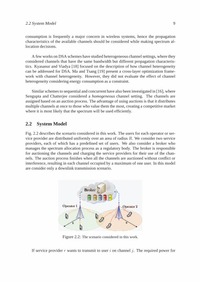
Fig. 2.2 describes the scenario considered in this work. Theusers for each operator or ser-vice provider are distributed uniformly over an area of radiusR. We consider two serviceproviders, each of which has a predefined set of users. We alsoconsider a broker whomanages the spectrum allocation process as a regulatory body. The broker is responsiblefor auctioning the channels and charging the service providers for their use of the chan-nels. The auction process finishes when all the channels are auctioned without conflict orinterference, resulting in each channel occupied by a maximum of one user. In this modelare consider only a downlink transmission scenario.

Figure 2.2:The scenario considered in this work.

If service providerr wants to transmit to useri on channelj. The required power for


service providerr to reach useri, with a fixed signal to noise (SNR) that guarantees thequality of the link, is given as:

P(r,i,j) = Co (dr,i)α (fj)

2 , (2.1)

whereCo is a constant computed from the SNR threshold, noise power, and the speed oflight; dr,i is the distance between the base station of service providerr and the useri; andfj is the frequency of channelj. Note, the the propagation loss model used is free spacepropagation.

We defineU(r,i,j), as the utility that service providerr achieves by serving useri onchannelj, by:

U(r,i,j) = xuser − Ccost(j) −K P(r,i,j), (2.2)

wherexuser is a fixed price that each user pays for the service,Ccost(j) is the cost for usingchannelj in monetary unitsand,K is the cost for energy inmonetary unit/power unit.

The utility function is a decision-taking tool that the service providerr uses to chooseif a user can be served, such that for a useri to be served thenU(r,i,j) > 0. The utilityfunction capturesK as a parameter in order to represent two scenarios: a situations whereservice providers have limited coverage due to expensive energy (highK) and when ser-vice providers have high coverage due to inexpensive energy(low K), in the last case theservice providers are not restricted to serve only near by users.

2.3 Mechanism Description

In this work, we consider two distributed DSA mechanisms,sequentialandconcurrentspectrum access, that take into account the different propagation characteristics and powerrequirements of different channels.

Thesequentialspectrum access mechanism is based on a sequential ascending auction.The broker offers the channels one by one on an individual basis, raising the price of thechannel until no more than one operator is willing to pay the price. The competition isexecuted for one channel without any information about the likely price for the followingchannels.

The concurrentspectrum access mechanism is carried out by iterative combinatorialauction. The operators bid for a set of different channels, computing the bestuser-channelcombinations, solving the optimization problem defined in equation 2.3, wherea(r,i,j) is 1if useri gets channelj, andzero otherwise.

Max

I,J∑

i,j

a(r,i,j)U(r,i,j). (2.3)

2.4 Results 11

This optimization problem has the constraint that for any user i a maximum of one channelshould be assigned

R,J∑

r,j

a(r,i,j) ≤ 1, (2.4)

and that any channelj cannot be allocated to more than one user,

I∑

i

a(r,i,j) ≤ 1. (2.5)

The performance of the two considered mechanisms is compared with; (i) the central-ized allocation scheme which provides the upper bound; and (ii) the distributed homoge-neous channels scheme which provides the lower bound regarding spectrum utilization.

2.4 Results

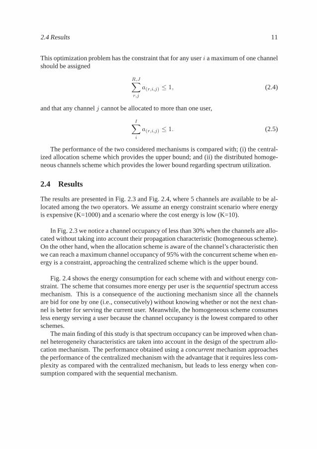
The results are presented in Fig. 2.3 and Fig. 2.4, where 5 channels are available to be al-located among the two operators. We assume an energy constraint scenario where energyis expensive (K=1000) and a scenario where the cost energy islow (K=10).

In Fig. 2.3 we notice a channel occupancy of less than 30% whenthe channels are allo-cated without taking into account their propagation characteristic (homogeneous scheme).On the other hand, when the allocation scheme is aware of the channel’s characteristic thenwe can reach a maximum channel occupancy of 95% with the concurrent scheme when en-ergy is a constraint, approaching the centralized scheme which is the upper bound.

Fig. 2.4 shows the energy consumption for each scheme with and without energy con-straint. The scheme that consumes more energy per user is thesequentialspectrum accessmechanism. This is a consequence of the auctioning mechanism since all the channelsare bid for one by one (i.e., consecutively) without knowingwhether or not the next chan-nel is better for serving the current user. Meanwhile, the homogeneous scheme consumesless energy serving a user because the channel occupancy is the lowest compared to otherschemes.

The main finding of this study is that spectrum occupancy can be improved when chan-nel heterogeneity characteristics are taken into account in the design of the spectrum allo-cation mechanism. The performance obtained using aconcurrentmechanism approachesthe performance of the centralized mechanism with the advantage that it requires less com-plexity as compared with the centralized mechanism, but leads to less energy when con-sumption compared with the sequential mechanism.


1 2 3 4 5 6 7 8 9 10 11 12 1310

20

30

40

50

60

70

80

90

100

Sequential K=10Concurrent K=10Centralized K=10Sequential K=1000Concurrent & Centralized K=1000Homogeneous K=10Homogeneous K=1000

Cha

nnel

Occ

upan

cy[%

]

Number of users

Figure 2.3: Channel Occupancy in the system versus number ofusers. Notice that thehomogeneous mechanism gives less than 30% channel occupancy, while sequential andconcurrent mechanisms approach centralized performance.

1 2 3 4 5 6 7 8 9 10 11 12 13

10−2

10−1

100

Sequential K=10Concurrent K=10Centralized K=10Sequential K=1000Concurrent & Centralized K=1000Homogeneous K=10Homogeneous K=1000

Nor

mal

ized

Pow

erpe

rac

tive

user

Number of users

Figure 2.4: Power expended per each served user.

Chapter 3

Secondary Spectrum Access toMeteorological Radar Band

3.1 Introduction

We have previously discussed that there is a need for utilizing radio spectrum more effi-ciently. We discussed dynamic spectrum access (DSA) based on the open sharing modelas one possible solution to utilize the allocated spectrum more efficiently. In this chapter,we examine another DSA strategy based on secondary spectrumaccess (also called the hi-erarchical access model) which is envisioned by cognitive radio [10]. This strategy allowssecondary users to access the spectrum that has already beenassigned to primary users.The basic idea is that the secondary users should be capable of detecting opportunities forusing the allocated spectrum without causing harmful interference to the primary users.

It has been shown that the creation of unlicensed bands stimulate competition in themarket, allowing the entrance of more equipment vendors. Anexample is the unlicensedindustrial, scientific, and medical (ISM) radio band. The almost free use of this bandwith few restrictions for access, has created many personalwireless technologies such asBluetoothr, Wi-Fir, and other forms of WLAN, which are all quite popular. As result ofthis popularity, the ISM band is crowded and the current and emerging unlicensed tech-nologies are looking for others bands, as is the case for WLAN1. After a long period ofpreparation, the ITU at the World Radio Conference 2003 (WRC2003) [20] agreed thatWLAN devices can have access to the spectrum primarily assigned to radio detection andranging systems (radars) in the 5 GHz frequency band (5150-5350 MHz and 5470-5725MHz), but the radar should be protected from interference.

Therefore, some initiatives for avoiding harmful interference to the radars have emergedsuch as the ETSI standard 301 893 V1.5.1 [21] which specifies the thresholds and require-ments for WLANs as secondary devices, and the IEEE 802.11h standard which specifies

1This is also termed as radio local area network (RLAN) and wireless access system (WAS) in the literature.

13

14 Chapter 3. Secondary Spectrum Access to Meteorological Radar Band

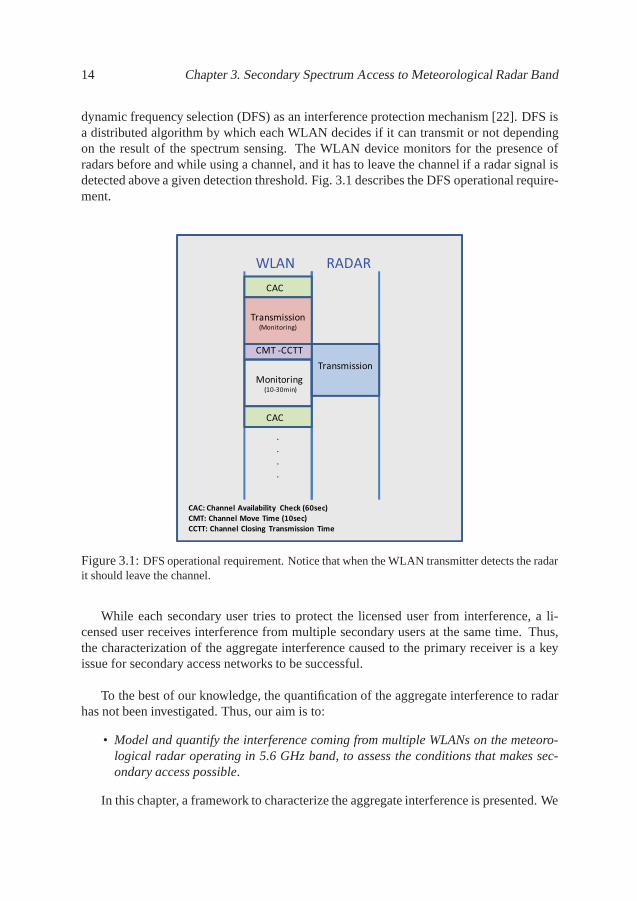
dynamic frequency selection (DFS) as an interference protection mechanism [22]. DFS isa distributed algorithm by which each WLAN decides if it can transmit or not dependingon the result of the spectrum sensing. The WLAN device monitors for the presence ofradars before and while using a channel, and it has to leave the channel if a radar signal isdetected above a given detection threshold. Fig. 3.1 describes the DFS operational require-ment.

WLAN RADAR

CAC

Transmission(Monitoring)

Transmission

CMT -CCTT

Monitoring(10-30min)

CAC

.

.

.

.

CAC: Channel Availability Check (60sec)

CMT: Channel Move Time (10sec)

CCTT: Channel Closing Transmission Time

Figure 3.1:DFS operational requirement. Notice that when the WLAN transmitter detects the radarit should leave the channel.

While each secondary user tries to protect the licensed userfrom interference, a li-censed user receives interference from multiple secondaryusers at the same time. Thus,the characterization of the aggregate interference causedto the primary receiver is a keyissue for secondary access networks to be successful.

To the best of our knowledge, the quantification of the aggregate interference to radarhas not been investigated. Thus, our aim is to:

• Model and quantify the interference coming from multiple WLANs on the meteoro-logical radar operating in 5.6 GHz band, to assess the conditions that makes sec-ondary access possible.

In this chapter, a framework to characterize the aggregate interference is presented. We

3.2 System Model 15

consider a meteorological radar2 as the primary or licensed user and WLAN as secondaryusers. However, the analytical framework can be adapted forother types of primary andsecondary users.

Related work

The quantification of opportunities for secondary access depends on the aggregate inter-ference created to the radar. Thus, a model to approximate the aggregate interference is animportant problem that we addressed.

In the related work to this problem, the authors of [23, 24] collected data from fieldexperiments, showing the degradation of the radar imagery caused due to the interferenceby WLAN. They concluded that enough protection can be provided by using dynamic fre-quency selection (DFS) for meteorological radar in 5.6 GHz.However, the measurementsdid not consider multiple interferers to characterize theaggregateinterference.

Various researchers in [25–28] have presented a mathematical model for the aggregateinterference in secondary access, where an exclusion region of a circle with a fixed radiusoffers the protection to the primary user from detrimental interference. However, the ex-isting models are not adequate for radar applications because the DFS mechanism is notproperly described by a circular exclusion regionin the presence of fading.

3.2 System Model

We consider a region of interference to the radar of radiusR, whereN uniformly dis-tributed secondary users in the region desire to transmit. The primary user is located at themiddle of the region. An illustration of the scenario is given in Fig. 3.2.

For each secondary transmitter to detect the primary receiver, we assume that eachsecondary transmitter can accurately estimate the propagation loss to the primary receiver.This is a reasonable assumption when a radar is the primary user, but can also be reason-able when the secondary users are assisted by a beacon signalfrom the primary receiver,in which case modifications of the primary receiver become necessary.

An individual secondary transmitter protects the primary receiver from interference byconsidering an interference thresholdIthr such that its transmission is prohibited if it wouldgenerate an interference higher thanIthr at the primary receiver. This is a distributed in-terference protection mechanism, similar to the DFS schemeemployed by WLAN devicesin 5GHz radar spectrum [22].

2From now on, thought the rest of the thesis, when we mentionedthe word “radar", we refer to the ground-based meteorological radar.


RB

-> Primary receiver -> Secondary transmi!er

*

**

**

*

** *

* *

*

*

*

*

*

*

*

*

*

*

** *

*

*

**

**

**

*

*

** *

**

*

**

*

* *

*

*

****

Figure 3.2:Deployment Scenario. The exclusion region has an irregularshape.

The probability density function (pdf) of the distributionof secondary users is given inequation 3.1, where a secondary userj is located at a distancerj from the primary user.

frj (y) =2y

R2, 0 < y ≤ R. (3.1)

Let us defineξj as the interference that the primary user would receive fromthe userj if itwere to transmit. Then,ξj is given by

ξj = G Pt L(rj) Xj , (3.2)

wherePt denotes the transmit power of the secondary user,Xj is a random variable(RV) modeling fading effect, andL(rj) is the distance-dependent path loss modeled asL(rj) = Crj

−α whereC is a constant andα is an exponent. The other gains and lossesare accounted for byG.

Let Ij be the interference from the userj which implements interference protection,thus the interferenceIj is regulated such that

Ij =

ξj , ξj ≤ Ithr,0, otherwise.

(3.3)

The aggregate interference model that we present is based onan interference threshold con-straint rather than in a exclusion region. Nevertheless, the interference threshold indirectlycreates an irregular exclusion region. Notice that the exclusion region model representsa situation where the secondary users know their distance from the primary receiver, butare ignorant of the propagation loss, e.g. they make use of a geo-location database of pri-mary users. Overall, it can be noted that the models based on interference threshold andexclusion region portray different levels of knowledge about the primary receiver.

3.3 Aggregate Interference Model 17

3.3 Aggregate Interference Model

Interference from an arbitrary secondary user

We focus first on finding the pdf ofξj . Observe from equation 3.2 thatξj is a functionof two random variables,rj andXj . Let us introduce a random variableUj denotingGPtL(rj) such thatξj = UjXj. The pdf ofUj is given by using equation 3.1, as:

fUj (u) =2

R2α

(

1

GPtC

)−2

α

u−2

α−1, Q ≤ u <∞, (3.4)

whereQ = GPtL(R). (3.5)

As for the fading effect, we consider shadow fading such thatXj follows a log-normaldistribution. By denoting the standard deviation of the shadowing byσdBXj using a dBscale, we have

fXj (x) =1

x√

2πσ2Xj

exp

[

−(lnx)2

2σ2Xj

]

, 0 < x <∞, (3.6)

whereσXj = σdBXj ln(10)/10.We assume the shadow fading does not depend on the location ofthe secondary user,

i.e. thatXj andUj are independent of each other. Then, the pdf ofξj can be expressed bythe following formula [29]:

fξj (z) =

∫

1

|x|fXj (x)fUj

( z

x

)

dx. (3.7)

The range ofx is obtained from (3.4). Thus, we have

fξj (z) =

∫ z/Q

0

Ψ

x2√

2πσ2Xj

exp

[

−(ln x)2

2σ2Xj

]

( z

x

)−2

α−1

dx. (3.8)

With a few mathematical manipulations, equation 3.8 can be simplified by using the Gaus-sian error function:

fξj (z) = Ωz−2

α−1

1 + erf

ln(z/Q)− 2σ2Xj/α

√

2σ2Xj

, (3.9)

where

Ω =1

R2α

(

1

GPtC

)−2

α

exp[

2σ2Xj/α

2]

. (3.10)

When interference protection is applied to equation (3.9),the transmission is allowedonly if ξj ≤ Ithr . This means there will be a portion of secondary users who arelimited to


zerotransmission power. That portion is given by1− Fξj (Ithr), whereFY (·) denotes thecumulative distribution function (CDF) of a random variableY . Thus, the pdf ofIj is:

fIj (z) =

1− Fξj (Ithr), z = 0,fξj (z), 0 < z ≤ Ithr,0, otherwise.

(3.11)

Aggregate interference

Let us defineIa as the aggregate interference fromN secondary users, which is given by:

Ia =

N∑

j=1

Ij . (3.12)

We employ a cumulant-based approach to approximate the pdf of Ia. Cumulants have anattractive property that theith cumulant of the sum of independent random varibles is equalto the sum of the individualith cumulants [28]. Also that the first and second cumulants ofa random variable correspond to the mean and variance. WhileEdgeworth expansion andshifted log-normal distribution have been proposed for theapproximation in the exclusionregion model [25], we found that a simple log-normal distribution describesIa well underthe considered interference protection.

Let κIa(i) be theith cumulant ofIa. Then,

κIa(i) =

N∑

j=1

κIj (i), (3.13)

whereκIj (i) is theith cumulant ofIj which can be easily computed from equation 3.11.By using the first two cumulants ofIa, the pdf ofIa can be approximated by the followinglog-normal distribution:

fIa(z) =1

z√

2πσ2Ia

exp

[

−(ln z − µIa)2

2σ2Ia

]

, (3.14)

where the parametersµIa andσ2Ia

can be computed from:

κIa(1) = exp[

µIa + σ2Ia/2

]

, (3.15)

κIa(2) =(

exp[

σ2Ia

]

− 1)

exp[

2µIa + σ2Ia

]

. (3.16)

3.4 Impact of the Aggregate Interference to Radar

Radar as a primary system

Some characteristics of radars create a propitious environment for sharing spectrum. Forexample, the low spatial utilization and narrow main beamwidth, allow secondary users

3.4 Impact of the Aggregate Interference to Radar 19

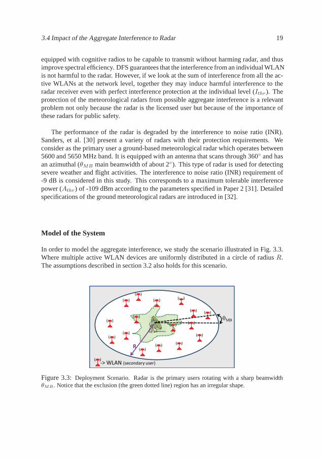
equipped with cognitive radios to be capable to transmit without harming radar, and thusimprove spectral efficiency. DFS guarantees that the interference from an individual WLANis not harmful to the radar. However, if we look at the sum of interference from all the ac-tive WLANs at the network level, together they may induce harmful interference to theradar receiver even with perfect interference protection at the individual level (Ithr). Theprotection of the meteorological radars from possible aggregate interference is a relevantproblem not only because the radar is the licensed user but because of the importance ofthese radars for public safety.

The performance of the radar is degraded by the interferenceto noise ratio (INR).Sanders, et al. [30] present a variety of radars with their protection requirements. Weconsider as the primary user a ground-based meteorologicalradar which operates between5600 and 5650 MHz band. It is equipped with an antenna that scans through 360 and hasan azimuthal (θMB main beamwidth of about 2). This type of radar is used for detectingsevere weather and flight activities. The interference to noise ratio (INR) requirement of-9 dB is considered in this study. This corresponds to a maximum tolerable interferencepower (Athr) of -109 dBm according to the parameters specified in Paper 2 [31]. Detailedspecifications of the ground meteorological radars are introduced in [32].

Model of the System

In order to model the aggregate interference, we study the scenario illustrated in Fig. 3.3.Where multiple active WLAN devices are uniformly distributed in a circle of radiusR.The assumptions described in section 3.2 also holds for thisscenario.

θMB

R

-> WLAN (secondary user)

(( ))

(( ))

(( ))(( ))

(( ))(( ))

(( ))

(( ))

(( ))

(( ))

(( ))

(( ))

(( ))

(( ))

(( ))

(( ))

(( ))

Figure 3.3: Deployment Scenario. Radar is the primary users rotating with a sharp beamwidthθMB . Notice that the exclusion (the green dotted line) region has an irregular shape.


Aggregate Interference model when radar is the primary receiver

The pdf ofξj andIj , can be computed using equations 3.9 and 3.11 with the differencethat:

G = GrGwOTR, (3.17)

whereGr is the radar’s maximum antenna gain,Gw is WLAN’s antenna gain, andOTRis the on-tune rejection factor defined as the ratio between the bandwidth of radarBr andthe bandwidth of WLANBw.

Now we express the aggregate interferenceIa fromN WLAN devices to the radar asfollows:

Ia =

N∑

j=1

Ijψ(θj), (3.18)

whereψ(·) is the antenna gain function of the radar andθj denotes the angle betweenWLAN j and the main beam of the radar antenna. We employ a simple antenna patternmodel of the radar. The maximum antenna gain of the radarGr is applied to WLANs thatare located within the main beamwidth denoted byθMB . A gain of zero dBi is applied toWLANs that are not insideθMB . In spite of its simplicity, our antenna pattern model givessimilar results those one suggested by ITU recommendation M.1652 [33]. We formallydefine the antenna pattern as:

ψ(θj) =

1, if θj < θMB1Gr, otherwise. (3.19)

The value ofθMB is approximated using the expressionθMB = 50[0.25Gr+7]0.5/10[Gr/20].The antenna elevation beamwidth is not used for simplicity,which lead to conservative re-sults.

As previously described, to approximate the PDF ofIa, we employed a cumulant-basedapproach. LetkIj (i) andkIa(i) denote theith cumulant ofIj andIa, respectively. Then,from equation 4.10 the following relationship is established for the first two cumulants:

kIa(1) =N∑

j=1

ψ(θj)kIj (1), (3.20)

kIa(2) =

N∑

j=1

ψ(θj)2kIj (2). (3.21)

A log-normal approximation is used to find the PDF ofIa as in equation 3.22, describedby the mean and the variance ofIj which can be easily calculated from equation 3.9.

fIa(z) =1

z√

2πσ2Ia

exp

(

ln(z)− µIa2σ2Ia

)

. (3.22)

3.5 Results 21

The parametersµIa andσ2Ia

of the PDF can be obtained from the first and second cumulantcomputation as shown is equations 3.15 and 3.16.

3.5 Results

The results presented in this section are from the scenario where WLAN shares spectrumwith a radar in the 5.6GHz band. We considered the radius of the interference regionRas 150Km. The antenna gain for radar is 40dBi and0 dBi for WLAN, also the bandwidthfor radar is 4MHz and 20MHz for WLAN. The standard deviation of the shadow fadingσdBXj is 8dB. We considered the radar’s antenna height to be 30 meters and 1.5 meters forWLAN’s antenna height. The aggregate interference threshold Athr is set to -109dBm toguarantee an INR=-9dB at the radar.

Verification of the Model

The mathematical framework is verifying by Monte Carlo simulation using the simulationtool MathWorks MATLAB. Fig. 3.4 shows the CDF of the aggregate interference whenthe WLAN user density is 1 per km2 andIthr = −109 dBm. Notice that the analysis hasa good match with the simulation, meaning that we can use a log-normal distribution tocharacterize Ia.

−95 −94.5 −94 −93.5 −93 −92.5 −92 −91.5 −910

0.1

0.2

0.3

0.4

0.5

0.6

0.7

0.8

0.9

1

SimulationAnalysis

Aggregate interference powerIa [dBm]

Cum

ulat

ive

Dis

trib

utio

nF

unct

ion

(CD

F)

Figure 3.4: CDF of aggregate interference.

Impact of the Ithr

In Fig. 3.5 we can see how different values forIthr affect the transmitting user. ForIthr=-120dBm about 36% of the users are not allowed to transmit, while this percentage increases


with higher thresholdsIthr.

−160 −150 −140 −130 −120 −110 −100 −900

0.1

0.2

0.3

0.4

0.5

0.6

0.7

0.8

0.9

1

ξj

Ij when I

thr=−109 dBm

Ij when I

thr=−120 dBm

Interference Power of a secondary user [dBm]

Cum

ulat

ive

Dis

trib

utio

nF

unct

ion

(CD

F)

Figure 3.5: CDF ofξj andIj for differentIthr.

Impact of the environment on the aggregate interference

Fig. 3.6 and Fig. 3.7 show the main results obtained in this study. In Fig. 3.6 we observethat the aggregate impact of multiple interferers is severein rural areas (as the path lossexponent of 2.5), thus we have two choices in order to keepIa below its threshold; eitherthe WLAN density has to be much lower than 1 per km2 or a margin for the individualinterference thresholdIthr has to be put in place. Meanwhile, an adverse impact of aggre-gate interference does not appear in urban environment (dueto a path loss exponent of 3.5)until the density of simultaneously transmitting WLANs reaches 10 WLANs per km2.

Fig. 3.7 presents the probability of transmission of a WLAN which is at a certain dis-tance from the radar. We observe that if the radar is placed inrural environment, less than0.15% of WLANs have access to the radar band when the distancefrom the radar is 50kmeven with the density of 1 per km2. In the case of an urban environment, a separation of5km from the radar is sufficient to prevent harmful interference even for 10 WLAN perkm2.

We investigated the impact of aggregate interference on ground-based meteorologicalradar operating in 5.6 GHz. We found that in an urban environment WLANs can accessradar bands without harming radar in contrast to the rural case. However, we should takeinto account that the aggregate interference greatly depends on the propagation environ-ment and WLAN density. This implies that accurate estimation of propagation loss iscrucial in determining the individual interference threshold for WLAN. Also, the value ofthe individual interference threshold should be adjusted according to the environment.

3.5 Results 23

2.2 2.4 2.6 2.8 3 3.2 3.4 3.6 3.8 4−130

−120

−110

−100

−90

−80

−70

Ithr

=−109 dBm

Density=1 user/Km2

Density=10 user/Km2

Density=20 user/Km2

Path loss exponent (α)

Agg

rega

teIn

terf

eren

ce[d

Bm

]

Figure 3.6: Effect of the path loss exponent on the aggregate interference when the individualinterference thresholdIthr = Athr=-109dBm.

1 5 10 15 20 25 30 35 40 45 50

0

0.1

0.2

0.3

0.4

0.5

0.6

0.7

0.8

0.9

1

Density=1 WLAN/Km2 α=2.5 Ithr

=−127.6dBm


=−109dBm


=−134.5dBm


=−111.3dBm

WLAN distance from the Radar [km]

Pro

babi

lity

oftr

ansm

issi

on

Figure 3.7:Probability of transmission as a function of the distance from the radar, with adjustableIthr such thatIa ≤ Athr.

Chapter 4

Temporal Secondary Spectrum Accessto Meteorological Radar Band

4.1 Introduction

In our work presented in Chapter 3, we explained a model that estimates the aggregateinterference from multiple secondary users uniformly spread over a large area. The modelquantifies the opportunity for a WLAN to access the 5GHz band without harming the radar.Thus, the concept of an adjustable individual interferencethreshold is introduced. A con-cern arises when we take into account the fact that in realityusers tend to gather morein some places than in other. For example, towns and cities have higher secondary usersdensity than rural areas.

In the scenario when multiple secondary users are spread over a large area, it is likelythat they are more concentrated in some areas than in others,simulating cities orhot zones.It is expected that the aggregate interference under heterogeneous distributions of sec-ondary users is different from that with uniformly distributed users particularly when theradar rotates with sharp beam width. But also, the interference to the radar will be differentdepending on the direction of the radar’s main beam. Thus, when the radar is not facinga hot zone it is possible to have more secondary users transmitting if the secondary usersuse a sensing mechanism that considers the radar’s antenna pattern. This idea leads to theterm temporal access opportunities, meaning that a WLAN has a temporal opportunity totransmit that may be at a higher rate while the radar is not facing it. Thus, the followingresearch questions are addressed:

• How is the aggregate interference affected if heterogeneous densities of secondaryusers are considered?

• How much transmission opportunity can be obtained for the secondary user by con-sidering radar’s antenna pattern in the sensing?

25

26 Chapter 4. Temporal Secondary Spectrum Access to Meteorological Radar Band

The modeling of the aggregate interference gets more challenging in the heterogeneousdistribution scenario because we have to model the variation of user density over a largearea, and also the variation in propagation loss. This chapter is divided into two part.First, we will explore the case when a hot zone (representinga city) with higher densityis located at a certain distance from the radar. We will also investigate the impact ofshaping parameters of the hot zone such as the distance from the primary receiver, densitydifference from the background, and size of the hot zone. In the second part, we quantifythe temporal opportunities for secondary user when radar’santenna pattern is consideredin the sensing.

4.2 Modeling of the heterogeneous secondary user density

A model to describe heterogeneous user distribution considering a large area consisting ofcities, towns, and rural areas is not easy. But to start this modeling, we can consider thatthe city’s population density is much higher than that of rural area, and that the numberof secondary users is proportional to the population density. Moreover, that the secondaryusers are homogeneously distributed within each city with it own density. Then, the hotzone or city can be modeled as an annulus sector, as shown in Fig. 4.1.

θH

RB

-> Primary receiver

2∆rH

-> Secondary transmi!er

*

**

**

*

** *

* *

*

*

*

*

*

*

*

*

*

*

** *

*

*

**

*

**

**

**

***

*

rH

**

*

** *

* **

***

**

**

**

***

*

*

*

Figure 4.1: Representation of the scenario. The hot zone model is modeled as an annulussector.

In this chapter, we investigate one hot zone and its impact onthe aggregate interfer-ence, given that extending the work to several hot zones withdifferent densities is trivial.The consideration of annulus sector to represent the hot zone, in the field of secondaryspectrum access, has already been studied. Rabbachin, et al. [34] consider a non-circulararea by aggregation of infinitesimal annulus sectors, and Aljuaid and Yanikomeroglu [35]

4.3 Part I. Aggregate Interference Model 27

investigate the impact of secondary field size by assuming anannulus sector area. Theadvantage of using the annulus sector is that the hot zone canbe molded to various shapesaccording to the three shaping parameters:rH , ∆rH , andθH , shown in Fig. 4.1. The dis-tance between the center of the hot zone and the primary user is rH , the length of the hotzone (depth) is2∆rH , and the central angle (width) is given byθH . The hot zone is thencharacterize by the distance, depth, width, and the density.

In our system model, we assume thatNB secondary users are homogeneously dis-tributed in a circle of radiusRB (background) andNH secondary users are homogeneouslydistributed within a hot zone. The densities of secondary users in the background and thehot zone areρB andρH , respectively, with (ρH > ρB). The primary receiver is located atthe middle of the background circle.

The basic propagation loss model used in this study is the C1-Suburban WINNERmodel proposed for 5GHz band by WINNER project [36]. The parameters of the propaga-tion model in dB scale are:

L(d) = 41.2036 + 3.5225 log10(d[meter]). (4.1)

4.3 Part I. Aggregate Interference Model

Distribution of the secondary users

Let us consider an annulus sector with inner radiusR1, outer radiusR2, and central angleθc. A circle can be regarded as a special case of the annulus sector. Thus, it can representboth the background area and the hot zone. For the case of the background area, thefollowing parameters are applied:R1 = 0, R2 = RB, andθc = 2π. As for the hot zone,the parameters areR1 = rH −∆rH ,R2 = rH +∆rH , andθc = θH . Note that the primaryuser is located at the origin of the background circle.

The location of an arbitrary secondary userj is denoted by(rj , θj), where the randomvariablerj is the distance from the primary user to the userj, and the random variableθjis the its angle. Since the userj is assumed to have the uniform distribution, the pdf theuser’s location is given by:

frj,θj (y, θ) =2y

(R22 −R

21)θ

, R1 < y ≤ R2, 0 ≤ θ ≤ θc. (4.2)

By assuming the primary and secondary users have omnidirectional antennas, equa-tion 4.2 can be simplified as

frj (y) =2y

(R22 −R

21), R1 < y ≤ R2. (4.3)



Note thatξj is defined as the interference that the primary user will receive from the trans-mission of secondary userj. Then,ξj is given by:

ξj = GPtL(rj)Xj , (4.4)

wherePt denotes the transmit power of the secondary user,Xj is a random variable mod-eling fading effects, andL(rj) is the distance depend path loss model defined as:

L(rj) = Crj−α, (4.5)

whereC andα are the path loss constant and exponent, respectively. The other gain andlosses are accounted byG.

We consider a log-normal shadow fading forXj and assume thatXj is independent ofrj . From the result in Paper 3 [37] and the pdf of the secondary userj in equation 4.3, it isstraightforward to show that the pdf ofξj , fξj (z), is derived as follows:

fξj (z) = h(z,R2)− h(z,R1), (4.6)

where

h(z, y) = Ωz−2

α−1

1 + erf

ln(

zGPtL(y)

)

−2σ2

Xj

α√

2σ2Xj

. (4.7)

In equation 4.16,σdBXj denotes the standard deviation of the shadowing in dB scale,and theconstantΩ is given by:

Ω =1

(R22 −R

21)α

(

1

GPtC

)−2

α

exp(

2σ2Xj/α

2)

. (4.8)

In order to obtain the pdf ofIj from fξj (z), we follow the steps in Paper 3 [37].WhenIthr is applied to userj, it stops transmission ifξj exceedsIthr. This means that aportion of secondary users havezerotransmission power. That portion of users is given as1−Fξj(Ithr) whereFξj (.) denote the cumulative distribution function (CDF) ofξj . Thus,the pdf ofIj is:

fIj (z) =

1− Fξj (Ithr), if z = 0fξj (z), 0 < z ≤ Ithr0, otherwise.

(4.9)

The derivedfIj (z) can be directly applied to both the background and the hot zonesecondary users by adjusting the parametersR1 andR2 as discussed in section 4.3.

4.3 Part I. Aggregate Interference Model 29

The pdf of the aggregate interference

Let us defineIBj andIHi as the interference from the secondary userj in the backgroundand the secondary useri in the hot zone, respectively. The pdf ofIBj andIHi are given inequation 4.9. Since we assume thatNB secondary users are uniformly distributed withinthe background area andNH uniform secondary users are within the hot zone, the totalinterference received at the primary user from the all secondary usersITa is computed as thesum of the aggregate interference from the users in the backgroundIBa and the aggregateinterference from the users in the hot zoneIHa .

ITa = IBa + IHa =

NB∑

j=1

IBj +

NH∑

i=1

IHi , (4.10)

We employ a cumulant-based approach to approximate the pdf of ITa . LetkIBa (m) andkIHa (m) denote themth cumulant ofIBa andIHa , respectively. Then,

kITa (m) = kIBa (m) + kIHa (m) (4.11)

=

NB∑

j=1

kIBj

(m) +

NH∑

i=1

kIHi

(m).

From the cumulants of theITa , the pdf ofITa can be approximated as a known distribu-tion by employing the method of moments. We use a log-normal distribution to approxi-mate the pdf ofITa as in equation 4.12.

fITa (z) =1

z√

2πσ2ITa

exp

(

ln(z)− µITa2σ2ITa

)

. (4.12)

The parametersµITa andσ2ITa

of the PDF can be obtained from the first and second cumulantcomputations as:

kITa (1) = E[ITa ] = exp[µITa + σ2ITa/2], (4.13)

kITa (2) = V ar[ITa ] = (exp[σ2ITa

]− 1) exp[2µITa + σ2ITa

]. (4.14)


4.4 Part II. “Temporal" opportunities for secondary access

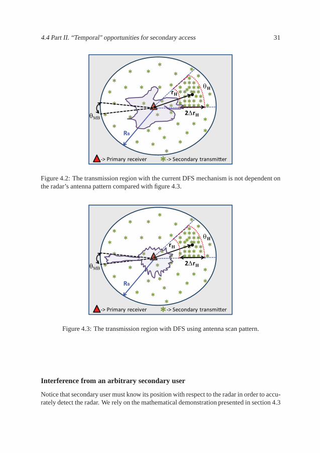
Introduction

The protection of the radar from detrimental interference is a constraint, in order for sec-ondary users to access radar’s band. The need to protect the radar led to the creation of theIEEE 802.11h standard which specifies dynamic frequency selection (DFS) as an interfer-ence protection mechanism. DFS is a distributed algorithm by which each WLAN decidesif it can transmit or not depending on the results of the spectrum sensing. Each WLANdevice monitors for the presence of a radar before and while using a channel, and it has toleave the channel if a radar signal is detected above a given detection threshold.

Fig. 4.2 shows the scenario when multiple WLANs are heterogeneously distributed.Each WLAN uses DFS in order to decide if it can transmit, without considering the radar’santenna pattern. Thus, the exclusive region remains the same independent of the radar’sscan pattern. Also, observe that the area where secondary users can not transmit is irregu-lar due to the fading effect. When a WLAN uses DFS as sensing mechanism and does notknow where the radar’s antenna is facing, it takes the decision on whether to transmit or notconsidering that the radar is facing it, even when may be not.This is not fair for the WLANwhich may has opportunity to transmits when the radar is not facing it. In contrast, Fig. 4.3shows that when DFS is applied including the radar’s antennapattern, termedtemporalDFS, the region where secondary users can not transmit is shapedaccording to the antennapattern, such that there is a larger exclusion region insidethe radar main beamwidth and ashorter exclusion region outside the main beamwidth. When the radar is not looking at thehot zone there would be greater use of the spectrum, because more users may be allowedto transmit with a higher data rate during that time. We note that there are temporal oppor-tunities for transmit if WLAN is aware of the radar’s antennapattern.

In this study we will compute the aggregate interference receive at the radar from thetransmission of multiple WLAN and quantify the number of active users. Two scenarioswill be studied: (1) Secondary users are uniformly spread over a large area and (2) Sec-ondary users gather creating heterogeneous user density. We note that when secondaryusers gather, the aggregate interference received at the radar increases, and even more soif the radar is facing the secondary users’ concentration. Therefore, in this part of ourwork, we implement a DFS mechanism which takes into account the radar antenna pat-tern, termedtemporal DFS. The basic idea is that each WLAN makes its own decision onwhether to transmit or not considering the current status, i.e., if it is facing the radar (max-imum interference) or not. A similar idea is proposed by Horváth and Varga [38], where achannel allocation technique is used by the WLAN users in order to eliminate interferenceto radars, but the study lacks a model and quantification of the aggregate interference andquantification of the spectrum utilization.

Our aim is to: Analyze and quantify how much transmission opportunity can be ob-tained for the secondary users for the four different cases?

4.4 Part II. “Temporal" opportunities for secondary access 31

θH

RB

-> Primary receiver

2∆rH


*

**

**

*

** *

* *

*

*

*

*

*

*

*

*

*

*

** *

*

*

**

*

**

**

**

***

***

*

** *

* **

***

**

**

**

***

*

*

*

*

*

* *****

***

rH

θMB

Figure 4.2: The transmission region with the current DFS mechanism is not dependent onthe radar’s antenna pattern compared with figure 4.3.

θH

RB

-> Primary receiver

2∆rH


*

**

**

*

** *

* *

*

*

*

*

*

*

*

*

*

*

** *

*

*

**

*

**

**

**

***

*

rH

**

*

** *

* **

***

**

**

**

***

*

*

*θMB

**

* **

***

Figure 4.3: The transmission region with DFS using antenna scan pattern.


Notice that secondary user must know its position with respect to the radar in order to accu-rately detect the radar. We rely on the mathematical demonstration presented in section 4.3


to directly compute the pdf ofξj as:

fξj (z) = h(z,R2, θj)− h(z,R1, θj), (4.15)

where

h(z, y, θj) = Ω(θj)z−2

α−1

1 + erf

ln(

zGr(θj)GwPtL(y)

)

−2σ2

Xj

α√

2σ2Xj

. (4.16)

In (4.16) the constantΩ(θj) is given by:

Ω(θj) =1

(R22 −R

21)α

(

1

Gr(θj)GwPtC

)−2

α

exp(

2σ2Xj/α

2)

. (4.17)

Equations 4.16 and 4.17 are dependent on the radar’s antennagainGr(θj) expressedas:

Gr(θj) =

Gmaxr , if 0 < θj ≤ θMB ,Gminr , otherwise.

(4.18)

whereGmaxr andGmaxr are the radar’s maximum and minimum antenna gain,θMB is theradar’s main beamwidth.

The pdf of the aggregate interference can be computed as shown in section 4.3.

4.5 Numerical Results

Part I

Notice that in section 4.3, we introduced a general mathematical framework to calculatethe aggregate interference, nevertheless when it comes to the simulation part we need todefine specific primary receiver and secondary users. Thus, we have specified a meteoro-logical radar as a primary receiver and WLANs as secondary transmitters. However, weassume that the primary receiver or the radar both have an omnidirectional antenna. Thisis because we do not compute the aggregate interference by snapshots (when the radar isfacing a portion of the total area), but assume the interference is independent of the direc-tion the radar is actually looking. This assumption leads toconservative results.

The next two simulations presented in Fig. 4.4 and Fig. 4.5 show the impact of thehot zone’s parameters(rH , and ∆rH ) on the aggregate interference. Two differentIthrare presented, one with a lower requirement for interference protectionIthr=-80dBm cre-ates a higher aggregate interference because 99.9% of the secondary users are allowedto transmit. The second simulation with a higher requirement for interference protectionIthr=-140dBm induces less aggregate interference to the primary receiver because only94.7% of the secondary users can transmit.

4.5 Numerical Results 33

5 10 15 20 25 30 35−105

−100

−95

−90

−85

−80

−75

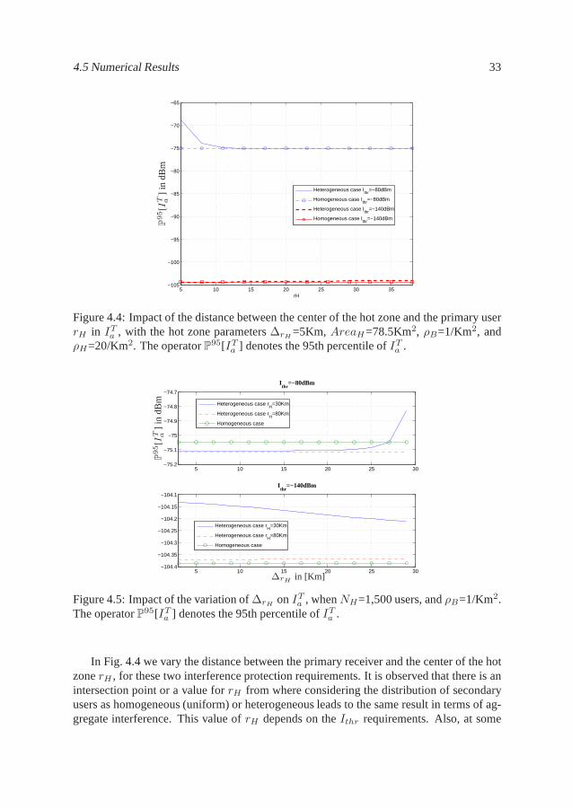
−70

−65

rH

Heterogeneous case Ithr

=−80dBm

Homogeneous case Ithr

=−80dBm

Heterogeneous case Ithr

=−140dBm

Homogeneous case Ithr

=−140dBm

P9

5[IT a

]in

dBm

Figure 4.4: Impact of the distance between the center of the hot zone and the primary userrH in ITa , with the hot zone parameters∆rH=5Km,AreaH=78.5Km2, ρB=1/Km2, andρH=20/Km2. The operatorP95[ITa ] denotes the 95th percentile ofITa .

5 10 15 20 25 30−75.2

−75.1

−75

−74.9

−74.8

−74.7

Ithr

=−80dBm

5 10 15 20 25 30−104.4

−104.35

−104.3

−104.25

−104.2

−104.15

−104.1

Ithr

=−140dBm

Heterogeneous case rH

=30Km


=80Km

Homogeneous case


=30Km


=80Km

Homogeneous case

∆rH in [Km]

P9

5[IT a

]in

dBm

Figure 4.5: Impact of the variation of∆rH onITa , whenNH=1,500 users, andρB=1/Km2.The operatorP95[ITa ] denotes the 95th percentile ofITa .

In Fig. 4.4 we vary the distance between the primary receiverand the center of the hotzonerH , for these two interference protection requirements. It isobserved that there is anintersection point or a value forrH from where considering the distribution of secondaryusers as homogeneous (uniform) or heterogeneous leads to the same result in terms of ag-gregate interference. This value ofrH depends on theIthr requirements. Also, at some


point of rH and highIthr considering the homogeneous distribution of secondary trans-mittersoverestimatesthe aggregate interference.

In Fig. 4.5 we show simulation results with different valuesfor the depth of the hotzone, but keepingrH fixed. This shows how the distribution of dispersion in the hot zone,rH − ∆rH < y ≤ rH + ∆rH , affects the aggregate interference when differentIthr arerequired. If the center of the hot zone is 80 Km away from the primary receiver, then avariation in∆rH does not affecting the aggregate interference. The opposite happens whenthe center of the hot zone is only 30Km away from the primary user. Then, the aggregateinterference increases or decreases (according toIthr) with an increment of∆rH . Thissuggests that the impact on the aggregate interference willdepend on the givenIthr, rH ,and∆rH .

Part II

In this section we present the results that quantify the number of WLAN that can accessthe radar band considering the four cases described in section 4.4. The heterogeneous dis-tribution is modeled considering a hot zone at 15 km from the radar, with∆rH=5Km andθH=10. The hot zone and background density areρH=20/Km2 andρH=1/Km2, respec-tively. Thus, in this work we consider 8,378 WLAN in total distributed within an area withradiusRB=50Km.

The temporal spectrum access opportunity for secondary users is quantify by measur-ing the percentage of active WLANs. Table. 4.1 presents the percentage of active WLANwhen DFS or Temporal DFS is used. When WLANs are heterogeneously distributed wecan observed a maximum difference in the percentage of active WLAN when DFS or Tem-poral DFS mechanism is considered, up to 5% more active WLAN when Temporal DFS isconsidered. The difference become smaller (0.83%) when a homogeneous distribution isconsidered. Notice that in general advance DFS mechanism allows more secondary usersto take advantage of the highly directional antenna that radar has by transmitting while theradar is not facing the WLAN.

Table 4.1: Percentage of Active WLANs

DFS Temporal DFSHomogeneous 99.15% 99.98%Heterogeneous 95% 99.76%-99.95%

The probability of transmission for a WLAN depending on the distance from the radaris shown in Fig. 4.6. We evaluated DFS and temporal DFS as interference protectionsmechanism. Observe that the users near to the radar have higher probability to transmitwhen the radar is not facing them and temporal DFS is used compared with the case whenDFS is used. When secondary users are heterogeneously distributed we can notice a dif-

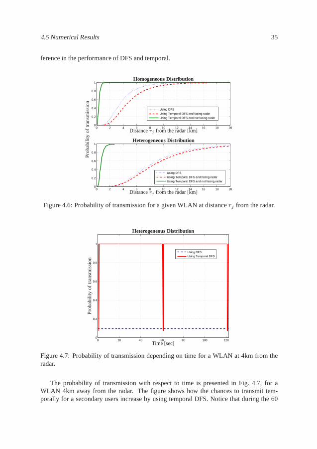
4.5 Numerical Results 35

ference in the performance of DFS and temporal.

0 2 4 6 8 10 12 14 16 18 200

0.2

0.4

0.6

0.8

1

Using DFSUsing Temporal DFS and facing radarUsing Temporal DFS and not facing radar

0 2 4 6 8 10 12 14 16 18 200

0.2

0.4

0.6

0.8

1

Using DFSUsing Temporal DFS and facing radarUsing Temporal DFS and not facing radar

Distancerj from the radar [km]

Distancerj from the radar [km]

Pro

babi

lity

oftr

ansm

issi

on

Homogeneous Distribution

Heterogeneous Distribution

Figure 4.6: Probability of transmission for a given WLAN at distancerj from the radar.

0 20 40 60 80 100 1200

0.2

0.4

0.6

0.8

1

Using DFSUsing Temporal DFS

Time [sec]

Pro

babi

lity

oftr

ansm

issi

on

Heterogeneous Distribution

Figure 4.7: Probability of transmission depending on time for a WLAN at 4km from theradar.

The probability of transmission with respect to time is presented in Fig. 4.7, for aWLAN 4km away from the radar. The figure shows how the chances to transmit tem-porally for a secondary users increase by using temporal DFS. Notice that during the 60


seconds that takes for the radar to rotate 360, the WLAN can transmit 99.45% of the timewith probability 1 when temporal DFS is used for heterogeneous distribution. Meanwhile,this probability is fixed all the time to 0.09 in the DFS case.

Chapter 5

Conclusions and Future Work

5.1 Concluding Remarks

The increasing demand for spectrum is forcing a change in thecurrent spectrum manage-ment model. Dynamic spectrum access models have been proposed as a solution. In thisthesis we address some challenges in the design of dynamic spectrum access models.

In Chapter 2 we considered an open sharing scenario which allocated the channels us-ing a market based mechanism. The channels are traded takingin to account each channel’spropagation characteristics, thus channels are considered heterogeneous. We used energyconsumption as a constraint. We evaluated two distributed mechanisms sequential andconcurrent access as in terms of channel usage and energy consumption. The main findingof the first part is that the channel occupancy increases whenchannel heterogeneity is con-sidered. Also we found that in wireless networks with energyconstraints the concurrentaccess mechanism consumes less power.

In Chapters 3 and 4 described a scenario where the spectrum isshared using hierarchi-cal access. The primary user is a radar and WLANs are secondary users. We demonstratean analytical framework to calculate the aggregate interference at the radar. We also presenta way to model the heterogeneous distribution of secondary users, termed hot zones. Fi-nally, we evaluated the temporal opportunities that WLANs have to access the radar’s band.From the analysis we found that: (1) The analytical approximation of the aggregate inter-ference, with homogeneous secondary user distribution andwith heterogeneous secondaryuser distribution, presents a good agreement with the simulation results. The frameworkcan help us easily calculate the probability of harmful interference generated by multiplesecondary users. (2) We also show that the aggregate interference at the radar is highlydependent on the propagation environment, being severe in rural areas. This suggests anaccurate estimation of the propagations loss is important.The value of individual interfer-ences threshold for WLAN is of importance, as a higher individual threshold prevents thisnode from transmitting. (3) The aggregate interference at the primary user is also greatly

37

38 Chapter 5. Conclusions and Future Work

affected by the heterogeneous density or concentration of secondary users when the hotzone is close to the primary receiver. Away from the primary receiver we can simplifythe model by not considering secondary user heterogeneity.(4) Finally, we show a incre-ment in the number of WLANs transmitting if Temporal DFS is employed as interferenceprotection mechanism which takes in to account the radar’s antenna pattern.

5.2 Future Directions

Possible directions for future work as an extension of this work include:

• In the aggregate interference model, the impact of fast fading remains interesting forfurther studies.

• In the hot zone model, an examination considering practical geographical regionsshould be done, to learn how the model can reflect the real environment. Also, theimpact of multiple hot zones could be investigated.

• We assume the WLANs can detect the radar and estimated the propagation lossaccurately. Thus, the evaluation of probability of miss detection and probability offalse alarm is still missing.

Bibliography

[1] ITU Report, “World Telecommunication/ICT DevelopmentReport (WTDR) 2010:Monitoring the WSIS Targets: A mid-term review,”International TelecommunicationUnion (ITU), 2010.

[2] J. A. Stine and D. L. Portigal, “Spectrum 101: An Introduction to Spectrum Man-agement,” MITRE CORP MCLEAN VA WASHINGTON C3I DIV, Tech. Rep., Mar2004.

[3] “Information Note to the Press (Press Release No. 28 /2010),” TELECOM REGULA-TORY AUTHORITY OF INDIA, Jun 2010.

[4] “Worldwide telecommunications industry revenues,”Internet Engineering TaskForce, Jun 2010.

[5] D. Cabric, I. O’Donnell, M.-W. Chen, and R. Brodersen, “Spectrum Sharing Radios,”IEEE Circuits and Systems Magazine, vol. 6, no. 2, pp. 30–45, 2006.

[6] M. A. McHenry, P. A. Tenhula, D. McCloskey, D. A. Roberson, and C. S. Hood,“Chicago spectrum occupancy measurements & analysis and a long-term studies pro-posal,” inTAPAS ’06: Proceedings of the first international workshop on Technologyand policy for accessing spectrum. New York, NY, USA: ACM, 2006, p. 1.

[7] V. Valenta, R. Marsalek, G. Baudoin, M. Villegas, M. Suarez, andF. Robert, “Survey on Spectrum Utilization in Europe: Measurements,Analyses and Observations,”INRIA a CCSD electronic archive serverbased on P.A.O.L [http://hal.inria.fr/oai/oai.php] (France). [Online]. Available:http://hal.archives-ouvertes.fr/hal-00492021/en/

[8] Federal Communications Commission Spectrum Policy Task Force, “Report of thespectrum efficency working group,” Tech. Rep., Nov. 2002, [Online]. Available:http://www.fcc.gov/sptf/reports.html.

[9] M. Wellens and P. Mähönen, “Lessons Learned from an Extensive SpectrumOccupancy Measurement Campaign and a Stochastic Duty CycleModel,” MobileNetworks and Applications, Springer Netherlands, vol. 15, pp. 461–474, 2010.[Online]. Available: http://dx.doi.org/10.1007/s11036-009-0199-9

39

40 BIBLIOGRAPHY

[10] J. Mitola III and G. Q. Maguire Jr, “Cognitive Radio: Making Software Radios MorePersonal,”IEEE Personal Communications, vol. 6, no. 4, pp. 13–18, Aug. 1999.

[11] E. Hossain, D. Niyato, and Z. Han,Dynamic Spectrum Access and Management inCognitive Radio Networks, 1st ed. Cambridge University Press, 2009.

[12] Q. Zhao and B. M. Sadler, “A Survey of Dynamic Spectrum Access: Signal Process-ing, Networking, and Regulatory Policy,”IEEE Signal Processing Magazine, vol. 24,no. 3, pp. 79–89, May 2007.

[13] M. A. McHenry, P. A. Tenhula, D. McCloskey, D. A. Roberson, and C. S. Hood,“Chicago Spectrum Occupancy Measurements & Analysis and a Long-term StudiesProposal,” inProc. of the 1st International Workshop on Technology and Policy forAccessing Spectrum (TAPAS ’06), 2006.

[14] O. Ileri, D. Samardzija, and N. Mandayam, “Demand responsive pricing and com-petitive spectrum allocation via a spectrum server,” inNew Frontiers in DynamicSpectrum Access Networks, 2005. DySPAN 2005. 2005 First IEEE International Sym-posium on, Nov 2005, pp. 194–202.

[15] S. Sengupta, M. Chatterjee, and S. Ganguly, “An Economic Framework for SpectrumAllocation and Service Pricing with Competitive Wireless Service Providers,” inNewFrontiers in Dynamic Spectrum Access Networks, 2007. DySPAN 2007. 2nd IEEEInternational Symposium on, April 2007, pp. 89–98.

[16] S. Sengupta and M. Chatterjee, “Sequential and Concurrent Auction Mechanismsfor Dynamic Spectrum Access,” inCognitive Radio Oriented Wireless Networks andCommunications, 2007. CrownCom 2007. 2nd International Conference on, Aug2007, pp. 448–455.

[17] S. Gandhi, C. Buragohain, L. Cao, H. Zheng, and S. Suri, “Towards real-time dy-namic spectrum auctions,”Comput. Netw., vol. 52, no. 4, pp. 879–897, 2008.

[18] P. Kyasanur and N. Viadya, “Protocol design challengesfor multi-hop dynamic spec-trum access networks,” inNew Frontiers in Dynamic Spectrum Access Networks,2005. DySPAN 2005. 2005 First IEEE International Symposiumon, nov 2005, pp.645–648.

[19] M. Ma and D. H. Tsang, “Joint design of spectrum sharing and routing with channelheterogeneity in cognitive radio networks,”Physical Communication, vol. 2, no.1-2, pp. 127–137, 2009. [Online]. Available: http://www.sciencedirect.com/science/article/B8JDV-4VT0XBP-1/2/5bc7358a2c1f2df45135eb6e4b0473a3

[20] The Wi-Fi Alliance, “Spectrum Sharing in the 5 GHz Band DFS Best Practices,”Tech. Rep., Oct. 2007.

BIBLIOGRAPHY 41

[21] ETSI EN 301 893 V1.5.1, “Broadband Radio Access Networks (BRAN); 5 GHz highperformance RLAN; Harmonized EN covering the essential requirements of article3.2 of the R&TTE Directive,” Dec. 2008.

[22] IEEE Std 802.11h-2003, “Spectrum and Transmit Power Management Extensions inthe 5 GHz band in Europe,” Oct. 2003.

[23] A. Brandao, J. Sydor, W. Brett, J. Scott, P. Joe, and D. Hung, “5 GHz RLAN Inter-ference on Active Meteorological Radars,” inProc. 61st IEEE Vehicular TechnologyConference (VTC), vol. 2, May 2005, pp. 1328–1332.

[24] P. Joe, J. Scott, J. Sydor, A. B. ao, and A. Yongacoglu, “Radio Local Area Network(RLAN) and C-Band Weather Radar Interference Studies,” inProc. 32nd AMS RadarConference on Radar Meteorology, Albuquerque, New Mexico, Oct. 2005.

[25] A. Ghasemi and E. S. Sousa, “Interference Aggregation in Spectrum-Sensing Cog-nitive Wireless Networks,”IEEE Journal of Selected Topics in Signal Processing,vol. 2, no. 1, pp. 41–56, Feb. 2008.

[26] A. Ghasemi, “Interference Characteristics in Power-Controlled Cognitive Radio Net-works,” in Proc. 5th International Conference on Cognitive Radio Oriented WirelessNetworks and Communications (CrownCom), Cannes, Jun. 9-11 2010.

[27] X. Hong, C.-X. Wang, and J. Thompson, “Interference Modeling of Cognitive RadioNetworks,” inProc. 67th IEEE Vehicular Technology Conference (VTC), Singapore,May 11-14 2008, pp. 1851–1855.

[28] M. Aljuaid and H. Yanikomeroglu, “A Cumulant-Based Characterization of the Ag-gregate Interference Power in Wireless Networks,” inProc. 71st IEEE VehicularTechnology Conference (VTC), Taipei, May 16-19 2010.

[29] A. Papoulis and S. U. Pillai,Probability, Random Variables, and Stochastic Pro-cesses, 4th ed. McGraw–Hill, 2002.

[30] F. H. Sanders, R. L. Sole, B. L. Bedford, D. Franc, and T. Pawlowitz, “Effects ofRF Interference on Radar Receivers, NTIA Report TR-06-444,” U.S. Department ofCommerce, Tech. Rep., September 2006.

[31] M. Tercero, K. W. Sung, and J. Zander, “Impact of Aggregate Interference on Meteo-rological Radar from Secondary Users,” inProc. IEEE WCNC, Cancun, Mar. 28–312011.

[32] Rec. ITU-R M.1638,Characteristics and protection criteria for sharing studies forradiolocation, aeronautical radionavigation and meteorological radars operating inthe frequency bands between 5250 and 5850 MHz, International TelecommunicationUnion Std., 2003.

42 BIBLIOGRAPHY

[33] Rec. ITU-R M.1652,Dynamic frequency selection (DFS) in wireless access systemsincluding radio local area networks for the purpose of protecting the radiodetermi-nation service in the 5 GHz band, Std., 2003.

[34] A. Rabbachin, T. Quek, M. Win, and H. Shin, “Cognitive Network Interference,”IEEE Journal on Selected Areas in Communications, vol. 29, no. 2, pp. 480–493,2011.

[35] M. Aljuaid and H. Yanikomeroglu, “Impact of Secondary Users Field Size on Spec-trum Sharing Opportunities,” inproc. IEEE WCNC, Sydney, Apr. 18–21 2010.

[36] IST-4-027756 WINNER II, “D1.1.2 v1.2 WINNER II ChannelModels,” [Online].Available: https://www.ist-winner.org/WINNER2-Deliverables/.

[37] K. W. Sung, M. Tercero, and J. Zander, “Aggregate Interference in Secondary Ac-cess with Interference Protection,”IEEE Communications Letters, 2011, accepted forpublication, temporariliy available at http://dl.dropbox.com/u/18150297/sung.pdf.

[38] Z. Horváth and D. Varga, “Channel allocation techniquefor eliminating interferencecaused by RLANs on meteorological radars in 5 GHz band,”INFOCOMMUNICA-TIONS JOURNAL, vol. LXIV, pp. 24–34, 2009.

Documents

Topics in Dynamic Spectrum Access