Embed Size (px)
Citation preview

Topics in Behavioral Economics
(Module MW21.6)
PD Dr. M. Pasche
Friedrich Schiller University Jena
Work in progress! Bug report to: [email protected]
p.1

Structure:
1. Introduction: Methodology of Behavioral Economics
2. Rational Choice Paradigm and its Limits
3. Other-regarding Preferences, Intrinsic Motivation,and Emotions
4. Reciprocity and the Impact of Beliefs
5. The Indirect Evolutionary Approach
6. Expectations and Fundamental Uncertainty
7. Rule-based Behavior and Rule Rationality
8. Policy Implications of Behavioral Economics
p.2

Preliminary schedule (summer 2018):
Week Tuesday Wednesday
15 Introduction ch.116 ch.2 ch.217 ch.2 ch.3
18 –∗) ch.319 ch.3 ch.320 ch.4 ch.521 ch.6 ch.622 ch.7 ch.723 ch.7 ch.824 exercise exercise25 exercise exercise26 exercise presentations27 presentations presentations28 presentations –
∗) public holiday
p.3

Type of course:
I Elective course in specialization areas “Innovation andChange” and “Economics and Strategy”
I 4 hours per week; 6 ECTS
Examination:
I Homework with presentation (50%)
I 60 min. endterm exam (50%)
p.4

Some selected introductory articles:
I Aumann, R. (1997), Rationality and Bounded Rationality. Games andEconomic Behavior 21, 2-14
I Conlisk, J. (1996), Why Bounded Rationality? Journal of EconomicLiterature Vol. 34, 669-700.
I Fudenberg, D. (2006), Advancing beyond “Advances in BehavioralEconomics”. Journal of Economic Literature 44(3), 694-711.
I Guth, W. (2007), (Non-)Behavioral Economics – A ProgrammaticAssessment. Jena Economic Research Papers No. 2007-099
I Kahneman, D. (2003), Maps of Bounded Rationality: Psychology forBehavioral Economics. American Economic Review 93(5), 1449-1475.
I McDonald, I.M. (2008), For the Student: Behavioural Economics. TheAustralian Economic Review 41(2), 222–228.
I Pesendorfer, W. (2006), Behavioral Economics Comes of Age: A ReviewEssay on Advances in Behavioral Economics. Journal of EconomicLiterature 44(3), 712-721
I Rabin, M. (2013), Incorporating Limited Rationality into Economics.Journal of Economic Literature 51(2), 528-543.
I Selten, R. (1990), Bounded Rationality. Journal of Institutional andTheoretical Economics Vol. 146, 649-658.
p.5

Some selected books:I Altman, M. (ed.) (2006), Handbook of Contemporary Behavioral
Economics: Foundations and Developments. Armonk, N.Y. and London:Sharpe.
I Camerer, C.F. (2003), Behavioral Game Theory: Experiments in StrategicInteraction. Princeton University Press.
I Cartwright, E. (2011), Behavioral Economics. Routledge.
I Dhami, S. (2016), Foundations of Behavioral Economic Analysis. OxfordUniversity Press.
I Kahneman, D. (2011), Thinking, Fast and Slow. New York: Farrar,Straus and Giroux.
I Just, D.R. (2014), Introduction to Behavioral Economics. Wiley
I Rubinstein, A., (1998), Modeling Bounded Rationality. Cambridge, Mass:MIT Press.
p.6

Requirements:
I It would be beneficial to have some knowledge in GameTheory.
I It would be beneficial to have some knowledge in Philosophyof Science, see slide collection “Approaches to EconomicScience – Part 2: What Is Social Science?”.
p.7

1. Introduction: Methodology of Behavioral Economics
Outline:
1.1 Methodological aspects of BE
1.2 Experimental Economics
1.3 Bounded Rationality
1.4 Interdisciplinarity
Literature:I Conlisk, J. (1996), Why Bounded Rationality? Journal of Economic
Literature Vol. 34, 669-700.
I Kahnemann, D. (2003), Maps of Bounded Rationality: Psychology forBehavioral Economics. The American Economic Review, 93, 1449-1475.
I Dhami, S. (2016), Foundations of Behavioral Economic Analysis. OxfordUniversity Press, Introduction (part 1-3).
p.8

1. Introduction: Methodology of Behavioral Economics1.1 Methodological aspects of BE
I Methodological individualism: economic activities andrelationships are based on individual choice behavior, shapedby institutions such like contracts, norms etc.
I Individual choice behavior depends on complexinterdependencies of goals and motives of individuals, theirinformations and beliefs, self-perception, social context, legaland institutional issues and so forth.
⇒ need for a (simplfying) model in order to explain/predictbehavior
I Models/theories based on “paradigms”, “research programs”or “explanatory styles”.
I Behavioral Economics focuses the empirical view on economicbehavior, and helps to create a better theoreticalunderstanding.
p.9

1. Introduction: Methodology of Behavioral Economics1.1 Methodological aspects of BE
Standard approach in (neoclassical) economics:
I Preferences: given and fixed; self-interest
I Choice set: given
I Beliefs: information about structure and parameters of thedecision environment shape beliefs about choice consequences⇒ beliefs are formed in a consistent way.
I Rational Choice: axioms on preferences about uncertainoutcomes⇒ representation of preference order⇒ choice behavior as maximization of expected utility.
I Equilibrium solutions
Sen, A. (1993), Internal Consistency of Choice. Econometrica 61, 495-522
p.10

1. Introduction: Methodology of Behavioral Economics1.1 Methodological aspects of BE
Although choice theory is often seen as descriptive, it is anexplanation since it basically follows the Hempel-Oppenheimscheme:
Explanans 1) Theory: Rational preferences; beliefs;
choice as expected utility maximization
2) Conditions: information set; choice set; payoffs
Explanandum 3) Conclusion: individual choice
p.11

1. Introduction: Methodology of Behavioral Economics1.1 Methodological aspects of BE
Recall “What is Social Science?” in module MW26.1:
I Internal validity is no problem as long as conclusions arederived from assumptions in a logically correct way.
I To be a scientific empirical theory or explanation,I the assumptions should not be counterfactual,I explanans should contain additional information,I theory should be empirically falsifiable.
I Thus, the “conclusions” in the scheme above could beconfronted with empirical data in order to test the underlyingtheory. Otherwise it is hard to qualify it as a scientific theoryas opposed to ideology or pseudo-science.
p.12

1. Introduction: Methodology of Behavioral Economics1.1 Methodological aspects of BE
I Further desirable properties: theory should be simple androbust.
I Simplicity : high comprehensibility and usefulness; “Occam’srazor”
I Robustness: no drastic changes in conclusions in case of somedeviations from the assumptions.
I However, both criteria are often conflicting.
p.13

1. Introduction: Methodology of Behavioral Economics1.1 Methodological aspects of BE
I If preferences and beliefs are well defined, if self-interest isassumed and the specific conditions are well defined, thenneoclassical choice theory (homo oeconomicus) makes clearpredictions.
I However, there are a lot of empirical “anomalies” (see chapter2) challenging the explanatory or predictive power of therational choice approach.
I How to respond to these empirical observations?
p.14

1. Introduction: Methodology of Behavioral Economics1.1 Methodological aspects of BE
Role of positive and normative theory:
Normative theory:
I independent from empirics
I general concepts, notions, methods for developing the logicalbasis of a description and explanation of choice behavior –such like preferences, rationality, consistency requirements
I principle of optimization behavior based on the “economicprinciple”
I defines the disciplinary borders of “economics”
Positive theory:
I based on normative theory
I description and explanation of observed behavior
I principle of falsification (Popper)
I experimental economicsp.15

1. Introduction: Methodology of Behavioral Economics1.1 Methodological aspects of BE
I The “as if” approach ⇒ unsatisfying.I Decomposing the explanans:
I Modifying the axioms on preferences, allowing for various sortsof biases, weighting functions, framing effects etc. (ch. 2)
I Modifying the content of preferences: e.g. other-regardingpreferences (ch. 3)
I State-dependent or belief-dependent preferences (ch. 4)I Extending the idea of “preferences” by including emotions,
moral norms, self-image etc. (ch. 3,4)
I Note: the structure of the economic explanation is still intact!Choice is still “rational” in the sense that it complies withconsistency requirements.
I Is it still the same research “paradigm” (Kuhn) or “core of aresearch program” (Lakatos)?
p.16

1. Introduction: Methodology of Behavioral Economics1.1 Methodological aspects of BE
I Bounded rationality and heuristic behavior :I No internal consistency required; choice behavior is not
portrayed as a form of maximization (substantial change of theexplanans).
I Rules, heuristics, adaptive behavior (ch. 7).I It is still required that individual want to achieve goals
(“utility”) but other choice principles such as satisificing arepossible (ch. 7).
p.17

1. Introduction: Methodology of Behavioral Economics1.1 Methodological aspects of BE
I Both routes are mixed up and discussed under the umbrella“Behavioral Economics”.
I Preference-based models maintain the rigorous explanatorystyle of economics. Questions arise:
I “Neo-classical repair shop” (W. Guth)?I Limits of falsifiabilityI But: elicits rich structured knowledge about preferences,
motives, psychological, and social conditions of choice.
I Boundedly rational models of heuristic behavior abandon theintellectual corset of the preference concept. Questions arise:
I Loss of generality or universality, lot of “local” theories; is itstill a genuine economic approach?
I Arbitrariness of assumptions: limits of falsifiabilityI On the other hand: this allows a broader notion of rationality
(e.g. rule rationality, ch. 7)
p.18

1. Introduction: Methodology of Behavioral Economics1.2 Experimental Economics
I BE is about empirically observed behavior and aims todevelop (better) positive theories.
I Problems with field data:I data availability, too short data setsI endogeneity of explanatory variablesI uncontrolled parameters (no “ceteris paribus” clause)I “controlled” field experiments possible but rare
I Experiments in the lab:I Ability to create large data setsI All parameters can be controlled and systematically variedI Flexible experimental design
I But:I Representativiness of participants?I External validity (behavior in the lab vs. behavior in real world)
p.19

1. Introduction: Methodology of Behavioral Economics1.2 Experimental Economics
Goals:
I Testing theories:
e.g. are the data consistent with theory X or theory Y? Createexperimental designs which discriminate whether X or Y hasmore explanatory power.
I Creating “stylised facts” (explanandum)⇒ inspiring new theories:
e.g. what happens with the behavior if parameter A iscontinuously varying? Which determinants have a positiveimpact on voluntary cooperation in public good games?
⇒ Interpreting the results could lead to modifications orextensions of theories or point to directions how to createalternative theories.
p.20

1. Introduction: Methodology of Behavioral Economics1.2 Experimental Economics
Testing theories: (cont.)
I Explanans: preferences, rationality, beliefs as unobservablepart; choice set, information conditions asobservable/controllable part
I Explanandum: Choice behavior to be explained
I Duhem-Quine problem: We are always testing jointhypotheses
I If results contradict the predictions thenI preferences may not satisfy the requirements, ORI beliefs are biased, ORI agents make not a rational choice but follow rules, ORI combinations of the mentioned reasons
I Limits of testabilty, limits of falsifiability
p.21

1. Introduction: Methodology of Behavioral Economics1.2 Experimental Economics
Example:
I Observing generous or cooperative behavior:
I Agents behave rational, but have socially motivatedpreferences (e.g. utility from monetary rewards of others).
I Agents are primarly self-interested but do not act accordingrational choice concept (non-expected utility theory ORrule-governed behavior etc.).
I Agents have simple preferences and act rationally but havedistorted beliefs regarding the behavior of other players.
I Not all reasons can always be disentangeld perfectly. Changesin experimental design can make some reasons more plausiblethan others. Example: The less the knowledge about thepayoffs of other players, the less “social preferences” are areasonable explanation.
p.22

1. Introduction: Methodology of Behavioral Economics1.2 Experimental Economics
Experimental Design:
I Not mimic the “reality”. Only few variables, and simpleconditions which can be properly understood by theparticipants.
I Design the rule so that only few explanations for the resultsare possible.
I Strategy Method : a strategy shows how the agent respondsto the (expected) behavior of other agents; in an experiment,however, you see only some few responses to specificsituations. Strategy method exhibits full range of responses toall possible situations. Problem: influences choice behavior.
p.23

1. Introduction: Methodology of Behavioral Economics1.2 Experimental Economics
I Repetition of games:I Enables learning of agents (better understanding of the rules
of the game, adaption of beliefs, learning how to make properchoices).
I Repetition with the same or with different partners.I Due to learning effects, observations may not be independent.
I Payment function:I Expected payments as large as the wage rate subjects can get
outside the lab.I Different decisions should have an non-negligible impact on the
payments.
I Clear Instructions
I Statistical analysis of the generated data
⇒ lectures by Prof. Kirchkamp!
p.24

1. Introduction: Methodology of Behavioral Economics1.3 Bounded Rationality
What does “rationality” mean?
The emergence of the standard concept of rationality ineconomics:
Already in the antique, philosophers asked about the reasons ofhuman behavior. A human being is characterized by therationalitas which enables her to reflect herself and theconsequences of her behavior. She will find arguments or reasonsfor her decisions, based on her reflexive abilities. The rationale fora decision is provided by sufficient reasons. Thus, rationaliy is usedin a much broader sense than the very specific concept ofconsistency (preferences obey certain axioms).
p.25

1. Introduction: Methodology of Behavioral Economics1.3 Bounded Rationality
I Adam Smith (1723-1790):I Agents are self-interested (egoistic), but are in some way
disciplinated by moral norms.I The ccordination of egoistic behavior by markets can lead to
collectively efficient and reasonable results (as opposed to thecontemporary belief that collective order must be providedagainst individual self-interest by central authorities/king)
I Decision making was not formalized
I Alfred Marshall (1842-1924) (at al.):I Establishes the notion of “utility” and “marginal utility”, as
introduced by Hermann Heinrich Gossen (1819-1858)I Not necessarily focussed on self-interest; a utility function can
contain everything.I Decision making was described by marginal calculus (Menger,
Jevons, Walras, Marshall); applying methods from classicalmechanics and mathematical optimization theory.
p.26

1. Introduction: Methodology of Behavioral Economics1.3 Bounded Rationality
I Modern expected utility theory:I von Neumann/Morgenstern (1947)I Different axiomatizations for preferences in order to derive
logically a utility function (under security and risk)I Rational choice: Behavior which is consistent with the axioms
so that expected utility is maximizedI Theory of revealed preferences
I Bounded rationality:I Herbert A. Simon (1950ies)I Broad empirical evidence against rational choiceI Also theoretical arguments for bounded rationality
(Simon, H.A. (1997), An Empirically Based Microeconomics. Cambridge:
Cambridge University Press [First Lecture]).
p.27

1. Introduction: Methodology of Behavioral Economics1.3 Bounded Rationality
Simple economic argument for Bounded Rationality:
I Cognitive resources are limited, hence informationprocessing and decision making bears cost.
I In the standard model these costs are neglected because itdeals with “ideal” agents with unlimited cognitive resources.
I These costs must be considered in order to judge whetherbehavior is “rational” or not.
I By doing so, it may turn out that simple rules instead ofmaximizing “perform better” – by means of the agent’s utilityfunction.
Problem:
I These deliberation costs itself are not observable (likepreferences). Does observed choice behavior reveal preferencesor deliberation costs?
p.28

1. Introduction: Methodology of Behavioral Economics1.3 Bounded Rationality
What does “bounded” mean?
I Bounded rationality is not irrationality.
I Limited cognitive abilities, limited information processingcapacities, limited awareness of new information, limitedmemory, stochastic errors
I What about other factors determining behavior such as: socialnorms, convictions, customs, emotions, reflexes?
I Are only the abilities affected which prevent agents fromperfect maximization, or does behavior also rely on principlesdifferent to maximization such like satisficing?
Langlois, R.N. (1990), Bounded Rationality and Behavioralism: A Clarificationand Critique. Journal of Theoretical and Institutional Economics 146, 691-695.
p.29

1. Introduction: Methodology of Behavioral Economics1.4 Interdisciplinarity
I Many relations to social psychology and cognitive psychology
I Emerging field: neuroeconomics – economic behaviorcorrelates with neurological states in the brain.
I Problem of different disciplinary “languages” (notions,concepts).
I Is there really a transfer of knowledge accross disciplinaryborders, or is it not more than a mutual inspiration?
I What is a specific economic explanation?I Gul, F., Pesendorfer, W. (2005), The Case for Mindless
Economics. Working paper (www.repec.org).I Pesendorfer, W. (2006), Behavioral Economics Comes of Age:
A Review Essay on ’Advances in Behavioral Economics’.Journal of Economic Literature Vol.44, 714-721.
p.30

2. Rational Choice Paradigm and its Limits
Outline:
2.1 Expected Utility Theory (EUT)
2.2 Empirical Problems
2.3 Methodological Problems
2.4 Modifications and Extensions: NEUT
Literature:I Fishburn, P.C. (1994), Utility and Subjective Probability, in: Aumann,
R.J., Hart, S. (eds.), Handbook of Game Theory 2. Amsterdam.
I Dhami, S. (2016), Foundations of Behavioral Economic Analysis. OxfordUniversity Press, chapter 1, parts of chapter 2.
I Kahneman, D. (2003), Maps of Bounded Rationality: Psychology forBehavioral Economics. American Economic Review 93(5), 1449-1475.
I Schmidt, T. (1995), Rationale Entscheidungstheorie und reale Personen.Marburg.
p.31

2. Rational Choice Paradigm and its Limits2.1 Expected Utility Theory
Preliminaries:
I Choices f1, f2, ... ∈ F (discrete oder continuous)
Example: drive slow, drive fastI Events A,B,C , ... ∈ S (to be discussed later on)
Example: clean street, oil on streetI Consequences x , y , z , ... ∈ E
⇒ Choices as functions which map possible events into the set ofconsequences:
fi : S → E
p.32

2. Rational Choice Paradigm and its Limits2.1 Expected Utility Theory
Example:
S
clean street oil on street
drive slow arrive late arrive very lateF
drive fast arrive in time arrive at hospital...
I Interpretation problem: If choice are characterized by identicalfunctions, i.e. fi (s) = fj(s) for all s ∈ S , then choices areidentical ⇒ not intuitive.
I Choices and consequences may be hard to disentangle ifchoices have an own value. Here, choices are seen purely in aninstrumental manner.
p.33

2. Rational Choice Paradigm and its Limits2.1 Expected Utility Theory
What is an event?
I Set of all environmental states Z .
I An event is a subset of Z , i.e. A,B, ... ⊆ Z .
I The set of events is the set of all subsets of Z= so-called σ-algebra on Z .
Example: throwing a dicePossible states: Z = 1, 2, 3, 4, 5, 6Possible events (examples):A =”‘pair”’ : 2, 4, 6B =”‘lower than 5”’ : 1, 2, 3, 4C =”‘unpair and greater than 4”’ : 5D =”‘greater than 7”’ : ∅E =”‘between 0 and 100”’ : 1, 2, 3, 4, 5, 6 = Z
p.34

2. Rational Choice Paradigm and its Limits2.1 Expected Utility Theory
I Probability of events:
P : S → [0, 1]
with the properties P(s) ≥ 0 ∀s ∈ S , P(S) = 1 andP(s1 ∪ s2) = P(s1) + P(s2) if s1 ∩ s2 = ∅.
p.35
2. Rational Choice Paradigm and its Limits2.1 Expected Utility Theory
I Security: The event is known ex ante (probability P = 1)
I Risk: Events are not known ex ante but there exists anobjective probability distribution on the set of all possibleevents.
I (Weak) Uncertainty: Events are not known ex ante butthere exist some subjective beliefs which are consistent withthe axioms.
I (Strong/Fundamental) Uncertainty: Events are not known(evtl. not defined) ex ante and it is not possible or reasonableto assign any probabilities to the events.
p.36

2. Rational Choice Paradigm and its Limits2.1 Expected Utility Theory
I Preferences: lat. prae-ferre = pre-fer.
An agent evaluates the consequences of a choice. If hedecides under risk or uncertainty, he evaluates the prospect ofpossible consequences (“lottery”).
We can only observe choices. If we see that an agent preferschoice A to B, then we may draw conclusions regarding theunderlying preferences and beliefs. If beliefs are known e.g.because probabilities are given, then the choice reveals thepreferences.
p.37

2. Rational Choice Paradigm and its Limits2.1 Expected Utility Theory
I Binary relation resp. :
An agent prefers X strictly over Y : X Y ,or he prefers X weakly over Y : X Y .
I A binary relation is rational (or a weak preference order)if
I Completeness: For all X ,Y ∈ M we have: X Y or Y Xor both (indifference X ∼ Y ).
I Transitivity: For all X ,Y ,Z ∈ M with X Y and Y Z wehave: X Z .
With one can define a strong preference order. But then werequire asymmetry : If X Y , then it is not Y X .
p.38

2. Rational Choice Paradigm and its Limits2.1 Expected Utility Theory
Utility function under security:
A weak preference order on the set M can be represented by autility function u : M → R, so that for all X ,Y ∈ M we have:
u(X ) ≥ u(Y ) ⇐⇒ X Y
This utility function is unique up to a positive-affine (orderpreserving) transformation.
(See Mas-Colell, A., Whinston, M.D., Green, J.R. (1995), Microeconomic
Theory. Oxford University Press, for a more elaborated derivation.)
p.39

2. Rational Choice Paradigm and its Limits2.1 Expected Utility Theory
I The resulting utility u(·) has to be interpreted as a utilityindex.
I It is a comfortable formal way to represent preferences. Thereis no psychological or motivational interpretation!
I Sometimes it is convenient to postulate certain properties ofthe utility function. Then we have additional requirements forM, e.g. convexity (will not be treated here).
p.40

2. Rational Choice Paradigm and its Limits2.1 Expected Utility Theory
I We are looking for a similar representation of preferences incase of uncertainty.
I Here, a choice does not have an unambigous consequence.We have to consider beliefs about possible events which leadto different consequences of the choice.
⇒ Lottery: A choice is now characterized by possibleconsequences and their probabilities.
Example:
L(”‘drive slow”’) = (p, ”‘late arrival”’; (1− p), ”‘very late arrival”’)L(”‘drive fast”’) = (p, ”‘arrival in time”’,(1− p), ”‘arrival at hospital”’)
with p as the probability of a clean street (no oil on street).
p.41

2. Rational Choice Paradigm and its Limits2.1 Expected Utility Theory
Lotteries:
I Simple lottery: L = (p1, ..., pn; x1, ...xn) with pi as theprobabilities for the possible choice outcomes x1, ..., xn.
I The outcomes xi are certain or, again, a lottery.
⇒ Compound lottery: Given k simple lotteries Lk andprobabilities αj then a compound lottery α1L1 + ..+ αkLkcorresponds with a simple lottery which gives the samedistribution over outcomes.
p.42

2. Rational Choice Paradigm and its Limits2.1 Expected Utility Theory
Preferences over lotteries:
I A weak preference order is now defined over the set oflotteries L.
I Continuity axiom: A preference relation over the set oflotteries L is continous if for all L1, L2, L3 ∈ L withL1 L2 L3 there exists a probability p so thatpL1 + (1− p)L3 ∼ L2.
I Independece axiom: A preference relation over the set oflotteries L satisfies the independence axiom if for allL1, L2, L3 ∈ L with L1 L2 and for all p ∈ (0, 1) we havepL1 + (1− p)L3 pL2 + (1− p)L3
In the latter case L3 is the so-called “irrelevant alternative” whichmakes no difference between the compound lotteries. In a similaraxiomatization this is also called the Sure Thing Principle.
p.43

2. Rational Choice Paradigm and its Limits2.1 Expected Utility Theory
Under the axioms of the weak preference order over L, thecontinuity axiom and the independence axiom there exists a utilityfunction u : L → R with
L1 L2 ⇐⇒ u(L1) ≥ u(L2)
for any L1, L2 ∈ L.
The utility function is of the expected utility form if the followingholds true: Let x1, ..., xn be the outcomes of a simple lottery Lwith probabilities p1, ..., pn. Then
u(L) = p1u(x1) + ...+ pnu(xn)
which also applies to lotteries: u(∑
i αiLi ) =∑
i αiu(Li ).This means that the expected utility function is linear in itselements (von Neumann/Morgenstern (1944)).
p.44

2. Rational Choice Paradigm and its Limits2.1 Expected Utility Theory
Stochastic Dominance:
I Assume that lotteries are characterized by their distribution ofa random variable X over the same range. Let F be thecumulative probability function.
I A lottery Y is first-order stochastically dominant over X ifFY (z) ≤ FX (z) for all z and FY (z) < FX (z) for at least onez . Or, alternatively: P(Y ≥ z) ≥ P(X ≥ z) for all z and “>”for at least one z . (Y has more chance than X to be largerthan any given value z .)
Important result: Assume that utility function u is monotonouslyincreasing. If lottery LY stochastically dominates lottery LX thenu(LY ) > u(LX ). Rational choice (maximizing expected utility)thus rules out (first-order) stochastically dominated alternatives.
p.45

2. Rational Choice Paradigm and its Limits2.1 Expected Utility Theory
Expected utility and utility of the expected value:
Assumption: The consequences X1,X2, ... are cardinal (e.g.monetary values). Then the utility function expresses the riskattitude of the agent.
Example: Lottery L = (p,X1; (1− p),X2) with X1 < X2 and thesecure outcome which equals the expected value of theconsequences: X = pX1 + (1− p)X2.
Risk neutrality: u(X ) = u(L) = pu(X1) + (1− p)u(X2)
Risk aversion: u(X ) > u(L) = pu(X1) + (1− p)u(X2)
Risk loving: u(X ) < u(L) = pu(X1) + (1− p)u(X2)
A risk-averse agent is willing to pay a risk premium in order tochange the risky lottery against the secure result.
p.46

2. Rational Choice Paradigm and its Limits2.1 Expected Utility Theory
u(r)
r (return)p(r)
r
u(E [r ])
E [r ]
E [u(r)]u(rs) =
rs
RP
p.47

2. Rational Choice Paradigm and its Limits2.1 Expected Utility Theory
Measuring the absolute risk aversion: Arrow-Pratt measure R
R(X ) = −u′′(X )
u′(X )= −d2u(X )/dX 2
du(X )/dX
measures the “concavity” of the utility function: the higher R the“more concave” is the function. It is a local measure since it isrelated to a certain point X .
Measuring the relative risk aversion: Arrow-Pratt measure r
r(X ) = −u′′(X )
u′(X )X = −d2u(X )/dX 2
du(X )/dXX
For a certain type of utility functions, r(·) is constant (CRRAfunctions). The risk premium RP is then a function of theArrow-Pratt measure. The expected utility E [u(X )] could then beapproximated by u(X − RP).
p.48

2. Rational Choice Paradigm and its Limits2.1 Expected Utility Theory
A graphical representation of expected utlity of lotteries:
I The axioms guarantee that expected utility is linear in theprobabilities. This leads to the following result:
I Let X ,Y ,Z be monetary payoffs with X < Y < Z (and acorresponding preference relation). We consider lotterieswhich differ only in their probability distribution pX , pY , pZ(with pX + pY + pZ = 1). Each lottery is then a point in theMachina triangle (see next slides).
p.49

2. Rational Choice Paradigm and its Limits2.1 Expected Utility Theory
Now consider two lotteries where the agent is indifferent:u(L1) = u(L2). Then we have:
u(L1) = u(L2)
p1Xu(X ) + (1− p1
X − p1Z )u(Y ) + p1
Zu(Z) = p2Xu(X ) + (1− p2
X − p2Z )u(Y ) + p2
Zu(Z)
p1X [u(X )− u(Y )] + p1
Z [u(Z)− u(Y )] = p2X [u(X )− u(Y )] + p2
Z [u(Z)− u(Y )]
(p1X − p2
X )[u(X )− u(Y )] = (p2Z − p1
Z )[u(Z)− u(Y )]
= (p1Z − p2
Z )[u(Y )− u(Z)]
dpX [u(X )− u(Y )] = dpZ [u(Y )− u(Z)]
dpXdpZ
=u(Y )− u(Z)
u(X )− u(Y )= const. (> 0)
As a result there exists a continuum of indifferently valuedlotteries. They must lie on a positively sloped line in the Machinatriangle. The steeper these indifference curves are, the higher isthe degree of risk aversion.
p.50

2. Rational Choice Paradigm and its Limits2.1 Expected Utility Theory
pZ
0 pX
1
1
L1 = (0.25,X ; 0.5,Y ; 0.25,Z)
L2 = (0.5,X ; 0,Y ; 0.5,Z)
L2
L1
0.5
0.5
0.25
0.25
L2 ∼ L1
L2
L1
L2 L1
L2
L1
p.51
2. Rational Choice Paradigm and its Limits2.1 Expected Utility Theory
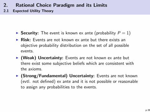
Alternative axiomatizations:
I The approach of von Neumann/Morgenstern requires acertain notion of “probability”.
I Other axiomatizations aim to deduce a probability concept, orthey imply different meanings of the underlying primitives, orthey represent them in a different formal way:
I Examples:I Savage, L.J. (1954), The Foundations of Statistics. New York.I Jeffrey, R.C. (1965), The Logic of Decision. Chicago.I Luce, R.D., Raiffa, H (1957), Games and Decisions. New York.I Marshak, K. (1959), Rational Behavior, Uncertain Prospects,
and Measurable Utility. Econometrica 18, 111-141.I Aumann, R.J. (1971), Utility Theory Without the
Completeness Axiom. Econometrica 30, 445-462.I Fishburn, P.C. (1964), Decision and Value Theory. New York.
p.52

2. Rational Choice Paradigm and its Limits2.1 Expected Utility Theory
Back to rationality:
I We call decisions rational if they can consistently berepresnted by the axioms of expected utility theory, i.e. agentschoose the most preferred alternative:
f ∗ ∈ arg maxf ∈F
∑si∈S
p(si )u(f (si ))
⇒ strong requirement⇒ very narrow interpretation of rationality.
I “Agents maximize their expected utility function” ⇒ there isno motivational or psychological interpretation, agents are notaware that they “have” a utility function. It is normativelogical representation of consistent (rational) choice.
I It is called ”‘substantive rationality”’ since there is no theoryhow a real decision making process works.
p.53

2. Rational Choice Paradigm and its Limits2.2 Empirical Problems
I Observed behavior in the lab deviates significantly andsystematically from the predictions of EUT. Thedeviations are often still present if participants are informedabout their inconsistent behavior, and when participantsaccept the assumptions (like transitivity) which they violate.
I The deviations depend on the experimental design. Thepossibility of learning and competitive pressure can sometimeshelp to move behavior into the direction of “rational” choice.
I In this chapter: we don’t consider empirical problems with riskjudgement (biases in risk percpetion, overconfidence, violationof Bayesian inference etc.) ⇒ chapter 6
Easy-reading introduction: Kahneman, D. (2011), Thinking, Fast andSlow. New York: Farrar, Straus and Giroux.
Extensive overview: Dhami, S. (2016), Foundations of Behavioral
Economic Analysis. Oxford University Press, chapter 19 and 20p.54

2. Rational Choice Paradigm and its Limits2.2 Empirical Problems
There are different axiomatizations of utility theory. All of themhave two requirements which are violated in lab and field:
I Transitivity of the preferences
I Sure-Thing-Principle (STP) (Savage 1954): Generalization ofwhat we have called “Independency from irrelevantalternatives”
If two choices f , g have identical consequences for a subset ofevents, A, then the preference relation f g can not dependon these events but from events from the complementary set¬A.
p.55

2. Rational Choice Paradigm and its Limits2.2 Empirical Problems
Allais paradoxon:(Allais, M., Hagen, O. (eds.) (1979), Expected Utility Hypotheses and the
Allais Paradox. Dordrecht.):
[Euro] pX = 0.01 pY = 0.1 pZ = 0.89
L1 100 100 100L2 0 500 100
L3 100 100 0L4 0 500 0
Choice set 1: L1, L2Choice set 2: L3, L4
p.56

2. Rational Choice Paradigm and its Limits2.2 Empirical Problems
Obviously we have:
L1(X ∪ Y ) = L3(X ∪ Y )
L2(X ∪ Y ) = L4(X ∪ Y )
L1(Z ) = L2(Z )
L3(Z ) = L4(Z )
I Both L1 and L2, as well as L3 and L4 have identical payoffs incase of event Z . Regarding the event X ∪ Y both pairs havethe same payoff structure.
I Consequently, it must be L1 L2 iff L3 L4 (or vice versa).
I But in the lab, a significant part of the participants chooseL1 L2, L4 L3 (or vice versa).
p.57

2. Rational Choice Paradigm and its Limits2.2 Empirical Problems
Ellsberg Paradoxon:Ellsberg, D. (1961), Risk, Ambiguity, and the Savage Axioms. Quarterly
Journal of Economics 75, 643-669.
Consider an urn with 30 red balls and 60 black and yellow ballswith unknown proportions. In contrast to the Allais experiment wehave no objectively given probabilities for “black” and “yellow”.
[Euro] red black yellow
L1 100 0 0L2 0 100 0
L3 100 0 100L4 0 100 100
Choice set 1: L1, L2Choice set 2: L3, L4
p.58

2. Rational Choice Paradigm and its Limits2.2 Empirical Problems
I A rational choice requires a subjective belief about theproportions of black and yellow balls.
I The most observed preference pair in experiments wasL1 L2; L4 L3, followed by L2 L1; L3 L4. Bothcontraticts the STP.
I Even if the contradiction to the STP is exemplified to theparticipants, a significant share of them was not willing torevise their choices.
I Possible explanation: Ambiguity aversion – in case of L1 andL4 the consequences of events with “unknown” probability areidentical, i.e. they do not depend on subjective expectation.
p.59

2. Rational Choice Paradigm and its Limits2.2 Empirical Problems
The “Certainty Effect”:
Consider three outcomes: x1 = 0, x2 = 3000, x3 = 4000 with theassociated probablities.
Choice problem A:
L1 = (x3 = 4000, p3 = 0.8; x1 = 0, p1 = 0.2)L2 = (x2 = 3000, p2 = 1)
Choice problem B:
L3 = (x3 = 4000, p3 = 0.2; x1 = 0, p1 = 0.8)L4 = (x2 = 3000, p2 = 0.25, x1 = 0, p1 = 0.75)
Most people choose L2 L1 and L3 L4.
p.60

2. Rational Choice Paradigm and its Limits2.2 Empirical Problems
This is a violation of the STP as it is:
L4 = 0.25L2 + 0.75 · 0L3 = 0.25L1 + 0.75 · 0
and “+0.75 · 0” is the “sure thing”.
This can be easily see in the Machina triangle because theconnection of L1 with L2 and l3 with L4 are parallel. Asindifference curves must be parallel, the observed preference paircannot be represented in a scheme of parallel indifference curve.
“Fanning out” phenomenon. Indifference curver become steeper(higher risk aversion) the higher the utility level is.
p.61

2. Rational Choice Paradigm and its Limits2.2 Empirical Problems
p1
p3
1
1
L1
L2
L3
L4
α α
fanning out
p.62

2. Rational Choice Paradigm and its Limits2.2 Empirical Problems
Framing effects:
I Kahneman, D., Slovic, P., Tversky, A. (eds.) (1982), Judgement underUnceretainty : Heuristics and Biases. Cambridge.
* Tversky, A., Kahneman, D. (1986), Rational Choice and the Framing ofDecisions. Journal of Business 59, 251-278.
I Loomes, G., Starmer, C., Sugden, R. (1991), Observing violations oftransitivity by experimental models. Econometrica 59, 425-439.
I Grether, D.M., Plott, C.R. (1979), Economic Theory of Choice and thePreference Reversal Phenommenon. American Economic Review 69,623-638.
Structurally identical choice problems should imply identical choicebehavior. The labelling of alternatives and the frame of presentingthe choice problem should not affect the rational choice. There is,however, significant evidence that framing may have a stronginfluence on the behavior.
p.63

2. Rational Choice Paradigm and its Limits2.2 Empirical Problems
Framing the risks:
Example: As a physician you have the following information aboutcancer therapy:
Problem 1 (framing in “gains”):
I Surgery: From 100 patients 90 survive the surgery, 68 survive up to1 year, and 34 survive up to 5 years.
I Radiation: From 100 patients all survive the time of radiation, 77survive up to 1 year, 22 survive up to 5 years.
Problem 2 (framing in “losses”):
I Surgery: From 100 patients 10 die during or immediately after thesurgery, 32 die within the next year, 66 die within the next 5 years.
I Radiation: From 100 patients none die in the time of radiation, 23die within the next year, and 78 die within the next 5 years.
p.64

2. Rational Choice Paradigm and its Limits2.2 Empirical Problems
Although the structure of risks and utility is identical in bothsettings, in setting 1 about 18% decide for radiation therapy, while44% decide for this therapy in setting 2 (Tversky/Kahneman1986).
⇒ asymmetric response to gains and losses: Not only thestructure but also the labelling and the absolute scale of outcomeshave an influence on behavior.
⇒ Prospect Theory(Kahnemann, D., Tversky, A. (1979), Prospect Theory: an analysis of decision
under risk. Econometrica 47, 263-291.)
p.65

2. Rational Choice Paradigm and its Limits2.2 Empirical Problems
Violating stochastic dominance:
Let L1 L3. Consider two differently composed lotteries.Rationality requires that the lottery is preferred which assigns themore preferred result a higher probability:
(p, L1, (1− p), L3) (w , L1, (1− w), L3)
iff p > w .
p.66

2. Rational Choice Paradigm and its Limits2.2 Empirical Problems
Problem 1:Option A 90% white 6% red 1% green 1% blue 2% yellow
0 +45 +30 -15 -15
Option B 90% white 6% red 1% green 1% blue 2% yellow
0 +45 +45 -10 -15
Obviously it is B A, which is chosen by the majority ofparticipants.
Problem 2:Option C 90% white 6% red 1% green 3% yellow
0 +45 +30 -15
Option D 90% white 7% red 1% blue 2% yellow
0 +45 -10 -15
p.67

2. Rational Choice Paradigm and its Limits2.2 Empirical Problems
I In problem 2 option C is identical with option A, because onlythe events ”‘blue”’ and ”‘yellow”’, which have the sameconsequences are subsumed to ”‘yellow”’.
I Option D is identical with option B because the events ”‘red”’und ”‘green”’ which have the same consequences aresubsumed to ”‘red”’.
I Thus, it is less obvious which alternative is dominant.
I Nevertheless, in problem 2 about 58% prefer option C(Tversky/Kahneman 1986).
p.68

2. Rational Choice Paradigm and its Limits2.2 Empirical Problems
Endowment effect:
I The higher the initial endowment, the higher is the aversionagainst possible losses. The utility of the endowment,however, should not affect choice since it is only an arbitraryshift of the utility index for all possible consequences.
I Induces systematic differences in WTP and WTA analysis.
⇒ Prospect Theory
Kahneman, D., Knetsch, J. L., Thaler, R. H. (2009), Experimental Tests of theEndowment Effect and the Coase Theorem. In E. L. Khalil (Ed.), The NewBehavioral Economics. Volume 3. Tastes for Endowment, Identity and theEmotions (pp. 119-142).
Carmon, Z., Ariely, D. (2000), Focusing on the Forgone: How Value Can
Appear So Different to Buyers and Sellers. Journal of Consumer Research
27(3), 360-370.
p.69

2. Rational Choice Paradigm and its Limits2.2 Empirical Problems
Influence of complexity and decision time:
I Deviations from rational choice increase with complexity ofthe problem.
I Deviations decrease with increasing decision time (but do notvanish).
I Deviations decrease with increasing monetary incentives (butdo not vanish).
(Wilcox, N.T. (1993), Lottery Choice: Incentives, Complexity, and Decision
Time. Economic Journal 103, 1397-1417.)
p.70

2. Rational Choice Paradigm and its Limits2.2 Empirical Problems
Social context and ability to logical conclusions:
Many experimental setups are very abstract. If the structure isenriched with a social context (using labels for persons, choices,outcome, and procedures from “real world”), then this contextualframing changes behavior. Agents are aware of a certain content,not only the formal structure.
Also the ability of participants to comprehend the structure of theproblem and to come to logical conclusions, may depend on thesemantic context.
Ortmann, A., Gigerenzer, G. (1997), Reasoning in Economics and Psychology:
Why Social Context Matters. Journal of Institutional and Theoretical
Economics 153(4), 700-710.
p.71

2. Rational Choice Paradigm and its Limits2.2 Empirical Problems
Wason Selection Task(Wason, P.C. (1966), Reasoning, in: Foxx, B. (ed.), New Horizons in
Psychology. Harmondsworth.)
Consider four cards and the following statement: “If there is avowel on the front side of the card, then the back shows an evennumber”. This statement should be proven by turning as few cardsas possible.
E K 7 2
p.72

2. Rational Choice Paradigm and its Limits2.2 Empirical Problems
Wason Selection Task with social context:(Griggs, R.A., Cox, J.R. (1983), The effects of problem content and negation in
Wason´s selection task. Quarterly Journal of Experimental Psychology 35A,
510-533.)
Statement which should be proven: “All persons who drink alcoholare at least 18 years old.”
drinksvodka
drinksjuice
22years
14years
p.73

2. Rational Choice Paradigm and its Limits2.2 Empirical Problems
Hyperbolic Discounting / Time-inconsistency
I Intertemporal choice problems: deciding in t = 0 about thecomplete path.
I Future utilities are (exponentially) discounted to the presentvalue, reflecting the impatience of the agent.
I A rational decision implies that the choice at every timepointis optimal, no incentive to deviate from the path.
I However, in case of hyperbolic discounting, the degree ofimpatience varies over time with a strong bias to the present.Hence, agents regret their earlier decisions and/or deviatefrom their path ⇒ behave in a time-inconsistent way.
I Examples: procrastination; too less savings for retirementphase; drug addiction.
O’Donghue, T., Rabin, M. (1999), Doing it now or later. American Economic
Review 89, 103-124.p.74

2. Rational Choice Paradigm and its Limits2.3 Methodological Problems
Empirical evidence makes it questionable to use EUT as a positivetheory of decision behavior.
How could EUT respond to these findings?
I Normative theory is intact, observed behavior is not rational.
I Modifying the underlying axiomatic framework, so that it haspositive explanatory power. Eventually estimating thedeviations from EUT?
I The underlying rationality principles are not empiricallytestable?
p.75

2. Rational Choice Paradigm and its Limits2.3 Methodological Problems
The problem of interpreting observations:
I The structure of the decision problem seem to be precisely definedby the experimentator. There are, however, possibleindividualisations which cannot be controlled perfectly. Theseindividualisations also determine how the decision problem isperceived by the participants. Examples:
I Not only the results, but also the circumstances how theoutcome was achieved, may have an influence on behavior.
I The choice action itself, not its outcome, may be valued.I Influence of the payoffs of other playersI Influence of emotions, social context
I An experimentator can try to control for such individualisations if heis aware of them. He can never be sure, however, that he is aware ofthe “complete” context of decision making.
p.76

2. Rational Choice Paradigm and its Limits2.3 Methodological Problems
Problem of falsifiability:
I One can only observe outcomes, not preferences or beliefs.
I If preferences and beliefs depend on variables which are not(yet) controlled in the experiment, then one can argue thattheory is intact since preferences and beliefs can be specifiedin a “proper” way.
⇒ Limits of falsifiability!
I However, in single agent choice experiments with monetarypayoffs, violations of axioms means that behavior isinconsistent with any preferences or beliefs. Thenon-falsifiability argument mainly applies to strategicinteraction, i.e. the notion of “social preferences”.
p.77

2. Rational Choice Paradigm and its Limits2.3 Methodological Problems
Problem of “logical omniscience” / fundamental uncertainty:
I Constructing an expected utility calculus requires a fullspecification of the decision problem (choice set, events,outcomes, beliefs have to be well defined).
I It is not necessary that the agent “knows everything”. If theagent is uncertain about something, he has to construct awell-defined set of possible states and a well-defined measureon this set. Outsiede the lab agents have to create a (mentalrepresentation of a) choice problem. Otherwise a calculus isnot possible.
I Impossibility to represent Fundamental Uncertainty.
p.78

2. Rational Choice Paradigm and its Limits2.3 Methodological Problems
Problem of reductionism:
I As mentioned above, many influences on decision behaviorcan be interpreted as part of (unobservable) preferences.Examples:
I Fairness as a social norm ⇒ preferences for fair allocationsI Emotions like envy ⇒ enter the utility functionI Bad conscience when taking an “unmoralic” action ⇒ enters
the utility function
I Is it reasonable to reduce everything to preferences? Why notconsidering social norms as a behavioral constraint? Why notinterpreting emotions as an additional explanatory devicewhich can modulate behavior even if preferences are stable?
p.79

2. Rational Choice Paradigm and its Limits2.3 Methodological Problems
The instrumentalistic interpretation of “choice”:
I Preferences are about (uncertain) outcomes. The choice itselfinduces these outcomes in a purely instrumental fashion.Preferring a choice f1 over f2 does therefore not mean thatthe choice act itself is valued.
I By this disjunction, it is hard or even impossible to implementethical issues where choices are valued independently fromtheir outcomes. Only emotional consequences (e.g. badconscience in case of unmoralic behavior, or disgust in case ofother’s unmoralic behavior) can be introduced as“preferences”.
(Vanberg, V.J. (2006), Rationality, Rule Following and Emotions: on the
Economics of Moral Preferences. Papers on Economics and Evolution No. 621,
Max Planck Institute of Economics, Jena.)
p.80

2. Rational Choice Paradigm and its Limits2.3 Methodological Problems
Dilemma:
I Very broad, contingent notion of “preferences”: almosteverything can be justified as “rational”, i.e. consistent with apreference order.
I Narrow notion of preferences: Variables influencing thebehavior are then additional determinants of choice besidepreferences. Observed behavior then does not necessarily“reveal” preferences.
Literature:I Schmidt, T. (1995), Rationale Entscheidungstheorie und reale Personen.
Marburg.
I Sen, A.K. (1977), Rational Fools: A Critique of the BehavioralFoundations of Economic Theory. Philosophy and Public Affairs 6,317-344.
I Tversky, A. (1975), A Critique of Expected Utility Theory: Descriptiveand Normative Considerations. Erkenntnis 9, 163-173.
p.81

2. Rational Choice Paradigm and its Limits2.3 Methodological Problems
Rationality and Intransitivity:
Why should rationality be based on strong restrictions on preferenceaxioms like transitivity? Those axioms enable an elegant consistentrepresentation of rational choice. But if an agent “refuses” to havewell-defined preferences, can we deny him rationality?
Example: fairy tale ”‘Hans im Gluck”’⇒ behavior is obviously not transitive⇒ it cannot be denied that Hans is a lucky person⇒ his choice behavior is subjectively beneficial
Example: “Desire to do something irrational” – preference for behavingnot consistently according to a preference order.
Example: “I am unlucky about my preference to smoke cigarettes.”
I Anand, P. (1993), The Philosophy of Intransitive Preference. EconomicJournal 103, 337-346.
I Sugden, R. (1985), Why be Consistent? A Critical Analysis ofConsistency Requirements in Choice Theory. Econometrica 52, 167-183.
p.82

2. Rational Choice Paradigm and its Limits2.3 Methodological Problems
Rationality and continuity axiom:
Even though continuity is intuitive at first sight, it may not beadequate in some situations. Example:
2Cent 1Cent death
It is not intuitive that any decision maker would prefer a lottery(p, 1Cent, (1− p), death) over 1 Cent.
⇒ lexicographic preferences
p.83

2. Rational Choice Paradigm and its Limits2.3 Methodological Problems
A compact overview about empirical and theoretical objectionsagainst standard rationality approach can be found in
I Conlisk, J. (1996), Why Bounded Rationality? Journal ofEconomic Literature 34, 669-700.
I Laville, F. (2000), Should we abandon optimization theory?The need for bounded rationality. Journal of EconomicMethodology 7(3), 395-426
p.84

2. Rational Choice Paradigm and its Limits2.4 Modifications and Extensions: NEUT
I A response to the empirical contradictions is to relax/modifythe axiomatic foundations of utility theory. The aim is, thatmore decision patterns can be consistently described asrational choice.
I The additional technical-mathematical effort is significant.
I Representation of the predictions of NEUT approaches byindifference curves in the Machina triangle.
I Due to modifications of the axiomatic framework, the utilityfunction will lose its property that the utility of a lottery canbe linearly decomposed to probability-weighted utilities ofsingle outcomes ⇒ Non-expected utility theory.
I Problem: NEUTs have more degrees of freedom to fit thedata. Theory must say what can not be observed. Predicitivepower of NEUT is remarkably low.
p.85

2. Rational Choice Paradigm and its Limits2.4 Modifications and Extensions: NEUT
Overview:
I Starmer, C. (2000), Developments in Non-expected UtilityTheory: The Hunt for a Descriptive Theory of Choice underRisk. Journal of Economic Literature 38(2), 332-382
I Kischka, P., Puppe, C. (1992), Decisions Under Risk andUncertainty: A Survey of Recent Developments. Methods andModels of Operations Research 36, 125-147.
I Machina, M. (1987), Choice Under Uncertainty: ProblemsSolved and Unsolved. Jourmal of Economic Perspectives 1,121-154.
I Machina, M. (1989), Dynamic Consistency and Non-ExpectedUtility Models of Choice Under Uncertainty. Journal ofEconomic Literature 27, 1622-1668.
p.86
2. Rational Choice Paradigm and its Limits2.4 Modifications and Extensions: NEUT
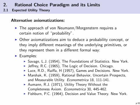
Few examples:
(a) Local Utility Functions(Machina, M. (1982), ‘Expected Utility’ Analysis Without the Independence
Axiom. Econometrica 50, 277-323.)
I Bundle/continuum of local utility functions.
I Using similar utility functions for similar decision problems,but different functions for different problems.
I Utility functions are not arbitrary, but vary in a “smooth” way(e.g. dependent on the payoff scale).
I Explaining the empirically relevant Fanning-Out phenomenonin the Machina triangle.
p.87

2. Rational Choice Paradigm and its Limits2.4 Modifications and Extensions: NEUT
pZ
0 pX
1
1
Fanning Out
pZ
0 pX
1
1
Fanning In
pZ
0 pX
1
1
Mixed Fanning
pZ
0 pX
1
1
Nonlinearindifference curves
p.88

2. Rational Choice Paradigm and its Limits2.4 Modifications and Extensions: NEUT
(b) Weighted Expected Utility(Dekel, E. (1986), An Axiomatic Characterization of Preferences under
Uncertainty — Weakening the Independence Axiom. Journal of Economic
Theory 40, 304-318. )
Relaxing the STP: Consider X Y . Then it is not necessary anylonger that pu(X ) + (1− p)u(Z ) ≥ pu(Y ) + (1− p)u(Z ) holdstrue for all p > 0, but there exists a (set of) q > 0 withpu(X ) + (1− p)u(Z ) ≥ qu(Y ) + (1− q)u(Z ), where p and q havea functional relation with certain properties. This leads to“weights” of the utilities of single outcomes:
V (L) =1∑
i piw(Xi )
∑i
piu(Xi )w(Xi )
with w(Xi ) as a weighting function for outcomes Xi .
p.89

2. Rational Choice Paradigm and its Limits2.4 Modifications and Extensions: NEUT
(c) Regret Theory(Loomes, G., Sugden, R. (1982), Regret Theory: An Alternative Theory of
Rational Choice under Uncertainty. Economic Journal 92, 805-824. )
The vaulations of the consequences of a choice are not independent anylonger. When valuating an outcome, the agent also reflects what hewould acchieve in case of another event. An unfavorable result inducestherefore a “regret”. This effect is captured by a pairwise comparison ofthe consequences which is weighted with a function of the probabilities ofthe different events. The regret about the unfavorable outcome will betypically lower if the probability of the event which induces the favorableconsequence, is extremely low:
V (L) =∑i
∑j 6=i
zj(pi , pj)v(Xi ,Xj)
with zj(·) as the weighting function.
p.90

2. Rational Choice Paradigm and its Limits2.4 Modifications and Extensions: NEUT
(d) Rank Dependent Utility(Quiggin, J. (1982), A Theory of Anticipated Utility. Journal of Economic
Behavior and Organisation 3, 323-343. )
I Not the utility of single outcomes, but the probabilities ofevents are weighted. Instead of the probabilities, a functiong : [0, 1]→ [0, 1] is used:
V (L) =∑i
g(pi )u(xi )
In case of a continous set of events the cumulativeprobabilities are weighted.
I With g(p) = p ∀p the EUT is included as a special case.
I This enables non-linear indifference curves in the Machinatriangle.
p.91

2. Rational Choice Paradigm and its Limits2.4 Modifications and Extensions: NEUT
(e) Prospect Theory(Kahnemann, D., Tversky, A. (1979), Prospect Theory: an analysis of decision
under risk. Econometrica 47, 263-291.)
This approach combines both, the weighting of probabilities andthe weighting of utilities of single outcomes according to a“reference point”.
Definitions:
I strictly positive prospect: all outcomes are positive
I strictly negative prospects: all outcomes are negative
I regular prospects: mixed
I “Positive” and “negative” is related to a reference point.
p.92

2. Rational Choice Paradigm and its Limits2.4 Modifications and Extensions: NEUT
Properties of the value function v(x):
I Defined for deviations from the reference point.
I Concave for gains and convex for losses.
I Steeper for losses than for gains.
Weighting function g(p(x)):
I g(0) = 0 and g(1) = 1
I g(p) > p for small p, g(p) < p for medium and large p
I Weights do not add up to one.
p.93

2. Rational Choice Paradigm and its Limits2.4 Modifications and Extensions: NEUT
losses gains
v(x)
0
1
1
g(p)
p.94

2. Rational Choice Paradigm and its Limits2.4 Modifications and Extensions: NEUT
Formal description of Prospect Theory (PT):
V (L) =∑i
g(pi (xi ))v(xi )︸ ︷︷ ︸losses
+∑j
g(pj(xj))v(xj)︸ ︷︷ ︸gains
p.95

2. Rational Choice Paradigm and its Limits2.4 Modifications and Extensions: NEUT
Example: Consider a reference point of zero.
I Set G.1: 95% chance to win 10,000, 100% chance to win 9,499:
g(0.95)v(10000) < v(9499)
⇒ risk averse because of concavity of v .
I Set G.2: 5% chance to win 10,000, 100% to win 501:
g(0.05)v(10000) > v(501)
⇒ risk seeking because of overweighting of unlikely events.
I Set L.1: 95% chance to lose 10,000, 100% chance to lose 9,499:
g(0.95)v(−10000) > v(−9499)
⇒ risk seeking because of convexity of v .
I Set L.2: 5% chance to lose 10,000, 100% to lose 501:
g(0.05)v(−10000) < v(−501)
⇒ risk averse because of overweighting of unlikely events.p.96

2. Rational Choice Paradigm and its Limits2.4 Modifications and Extensions: NEUT
Problem:
I It turned out that in PT choice A may be preferred to B evenif A is stochastically dominated by B. PT predicts more oftensuch violations than being empirically observed.
I By using a weighting function for cumulative probability like inRank-Dependent Utility Theory, this problem can be avoided.
⇒ Cumulative Prospect Theory (CPT)
p.97

2. Rational Choice Paradigm and its Limits2.4 Modifications and Extensions: NEUT
Cumulative Prospect Theory(Tversky, A., Wakker, P. (1993), An Axiomatization of Cumulative Prospect
Theory. Journal of Risk and Uncertainty 7, 147-176. )
For the case of continous events x and a reference point of zero wehave
v(L) =
∫ 0
−∞v(x)
d
dx(w(F (x)))dx +
∫ ∞0
v(x)d
dx(−w(1−F (x)))dx
where F (x) is the cumulative probability = integral of the densityfunction up to x .
p.98

2. Rational Choice Paradigm and its Limits2.4 Modifications and Extensions: NEUT
Problems:
I More behavioral patterns can now be described as consistentwith a NEUT approach. Does the latter “explain” thebehavior?
I Due to more degrees of freedom in designing weightingfunctions etc., the model can be fitted to more data, but isalso consistent with non-observed behavioral patterns. Thus,the predicitve power is limited.
I Model with best parameter fits in one context are performingbad in other contexts ⇒ functional forms and parameterscannot be generalized.
Neilson, W., Stowe, J. (2002), A Further Examination of Cumulative
Prospect Theory Parameterizations. Journal of Risk and Uncertainty
24(1), 31-46.
p.99

2. Rational Choice Paradigm and its Limits2.4 Modifications and Extensions: NEUT
I Empirical tests of several NEUT show disappointing results,see e.g.:
Literature:
I Harless, D.W., Camerer, C.F. (1994), The Predictive Utility ofGeneralized Expected Utility Theories. Econometrica 62, 1251-1289.
I Hey, J.D., Orme, C. (1994), Investigating Generalizations ofExpected Utility Theory Using Experimental Data. Econometrica62, 1291-1326.
p.100

2. Rational Choice Paradigm and its Limits2.4 Modifications and Extensions: NEUT
Idea:
If behavior could be well described by a NEUT model (parameterfitted to observed data): can we draw conclusions regarding theunderlying “true”, “unbiased”, “rational” preferences from EUT?
⇒ enables the external observer to frame the decision problem orto “nudge” the decision maker in a way that resulting behavior ismore close to her “true” preferences.
⇒ ?
Pinto-Prades, J.-L., Abellan-Perpinan, J.-M. (2012), When normativeand descriptive diverge: how to bridge the difference. Social Choice andWelfare 38, 569-584.
p.101

3. Other-regarding Preferences, Intrinsic Motivation, and Emotions
Outline:
3.1 Fairness, Cooperation, Trust, and Morale
3.1.1 Ultimatum and Dictator Game: Altruism, Envy, Fairness3.1.2 Public Good Games: Voluntary Cooperation and Reciprocity3.1.3 Trust and Trustworthiness3.1.4 Markets and Morale
3.2 Modelling Social Preferences
3.3 Emotions, Intrinsic Motivation, Self-Image
Literature:I Camerer, C.F. (2003), Behavioral Game Theory: Experiments in Strategic
Interaction. Princeton University Press.
I (More detailed sources will be given in the sections)
p.102

3. Other-regarding Preferences, Intrinsic Motivation, and Emotions3.1 Fairness, Cooperation, Trust, and Morale3.1.1 Ultimatum and Dictator Game: Altruism, Envy, Fairness
Ultimatum Game: Allocation of fixed F
X Y
proposal
(qx , qy = F − qx)
agree(qx , qy )
reject(0, 0)
I Basic structure of bargaining
I Subgame perfect equilibrium: proposal [qX = F − ε, qY = ε]with ε ≥ 0 near zero, and acceptance of the responder.
I Observe, that all allocations are pareto-efficient.
p.103

3. Other-regarding Preferences, Intrinsic Motivation, and Emotions3.1 Fairness, Cooperation, Trust, and Morale3.1.1 Ultimatum and Dictator Game: Altruism, Envy, Fairness
I One of the most explored experimental games –extremely broad literature
I Some older sources for an overview:
I Guth, W. (1995), On ultimatum bargaining – A personal review. Journalof Economic Behavior and Organization Vol. 27, 329-344.
I Guth, W. (2001), How ultimatum offers emerge – A study in boundedrationality. Homo Oeconomicus Vol. XVIII (1), 91-110.
I Kirchsteiger, G. (1994), The Role of Envy in Ultimatum Games. Journalof Economic Behavior and Organization 25, 373-390.
I Ochs, J., Roth, A. (1989), An Experimental Study of SequentialBargaining. American Economic Review 79, 355-384.
p.104

3. Other-regarding Preferences, Intrinsic Motivation, and Emotions3.1 Fairness, Cooperation, Trust, and Morale3.1.1 Ultimatum and Dictator Game: Altruism, Envy, Fairness
Some “stylized facts”:
I No proposals for the responder more than 50% of F .
I The majority of qY -proposals (ca. 60-80%) is in the interval[0.4F , 0.5F ]. On average the proposer receives qX = 0.6F .
I The fraction of qY -proposals in the interval [0, 0.2F ] (near theNash solution) is negligibly small.
I qY -proposals which are significantly below 50% of F will berejected with increasing probability. Proposals withqX > 2/3F are more often rejected than accepted.
p.105

3. Other-regarding Preferences, Intrinsic Motivation, and Emotions3.1 Fairness, Cooperation, Trust, and Morale3.1.1 Ultimatum and Dictator Game: Altruism, Envy, Fairness
Possible explanations:
I Proposer allocates significant payoffs to the responder:altruism, generosity?
I If agents are altruistic/generous, then responder would acceptany proposal. This is clearly not the case.
I If agents are altruistic/generous, then proposer would begenerous also in the dictator game (no veto of the responderis possible). But here they are much less generous.
I Responders reject very unequal allocations: envy? Punishingthe “unfair” proposer is preferred to small positive payoffs.
I Proposer anticipates envious behavior and offers significantshares.
I Envy as an emotion might be based on “fairness” concerns.
p.106

3. Other-regarding Preferences, Intrinsic Motivation, and Emotions3.1 Fairness, Cooperation, Trust, and Morale3.1.1 Ultimatum and Dictator Game: Altruism, Envy, Fairness
Variants of the Ultimatum Game
I Repeated Ultimatum Game with a “shrinking cake”:
I When Y has rejected, the cake to be allocated shrinks toδF , δ ∈ (0, 1). Player Y then makes a counter proposal(qY , qX = δF − qY ) which can be accepted or rejected by X .
I An envious Y has the chance to reverse the situation byrejection, but at the price that the cake to be allocated isshrinking. Moreover, he has to consider, that also X isenvious.
I Subgame perfect solution:I 2. stage: player X accepts any proposal, player Y demands
qY = δF − ε.I 1. stage: player Y accepts any proposal with qY ≥ δF − ε,
player X demands qX = (1− δ)F + ε.
p.107

3. Other-regarding Preferences, Intrinsic Motivation, and Emotions3.1 Fairness, Cooperation, Trust, and Morale3.1.1 Ultimatum and Dictator Game: Altruism, Envy, Fairness
Experimental results:
I On both stages the realized distributions are more equal thanin subgame perfect Nash solution.
I Too unequal proposals are rejected.
I There are unfavorable counter proposals with qY < δF − ε.
I Possible explanation: envy, fairness
I A simple model of envy can be found in Kirchsteiger (1994)
p.108

3. Other-regarding Preferences, Intrinsic Motivation, and Emotions3.1 Fairness, Cooperation, Trust, and Morale3.1.1 Ultimatum and Dictator Game: Altruism, Envy, Fairness
Different treatments: What drives the results?
I Role of communication
I Anonymous play vs. personal contact; knowing the name
I Scale of the payoff
I Effects of age, gender, and culture
I Influence of stochastic variables on the allocation
⇒ an unequal distribution is perceived as less “unfair” and envyplays a less role when allocation is affected by stochasticinfluences
⇒ Not the result itself, but the supposed intention of theproposer plays a role
I etc.
(Detailed literature given on demand.)
p.109

3. Other-regarding Preferences, Intrinsic Motivation, and Emotions3.1 Fairness, Cooperation, Trust, and Morale3.1.1 Ultimatum and Dictator Game: Altruism, Envy, Fairness
Dictator Game: Allocation of F without veto power
X
proposal
(qx , qy = F − qx)
(qX , qY )
Nash equilibrium: (qX = F , qY = 0)
p.110

3. Other-regarding Preferences, Intrinsic Motivation, and Emotions3.1 Fairness, Cooperation, Trust, and Morale3.1.1 Ultimatum and Dictator Game: Altruism, Envy, Fairness
Observation:
I Proposer give about 20% of F to the receiver although he hasno veto power.
I About 1/3 of the proposers choose the Nash solution.
Forsythe, R., Horowitz, J., Savin, N., Sefton, M. (1994), Fairness inSimple Bargaining Experiments. Games and Economic Behavior 6(3),347-369.
p.111

3. Other-regarding Preferences, Intrinsic Motivation, and Emotions3.1 Fairness, Cooperation, Trust, and Morale3.1.1 Ultimatum and Dictator Game: Altruism, Envy, Fairness
I Possible explanation: altruism, generosity? But why shouldthe degree of generosity depend on veto power?
I Envy can not play a role since X has no veto power.
I Combining the observations of Ultimatum and Dictator Game,neither envy nor altruism can explain all results, preferencesfor “fair” allocations can explain both.
I Fairness norms account not only for the degree of (in)equality,but also for the intentions and conditions how the allocation isachieved (differences in UG and DG).
p.112

3. Other-regarding Preferences, Intrinsic Motivation, and Emotions3.1 Fairness, Cooperation, Trust, and Morale3.1.2 Public Good Games: Voluntary Cooperation and Reciprocity
I Public Good:I Non-rivalry in useI Non-excludability from use
I This creates an incentive to free-riding, implying anunderprovision of the public good and hencepareto-inefficiency (positive externality).
I Special case: Prisoner’s Dilemma Game
I If all agents contribute to the public good, the allocation ispareto-efficient and the sum of payoffs is maximized. Butobserve that there exists many efficient allocations wheresome agents contribute while others are not; in the PD gameall outcomes except for the Nash solution are efficient.
p.113

3. Other-regarding Preferences, Intrinsic Motivation, and Emotions3.1 Fairness, Cooperation, Trust, and Morale3.1.2 Public Good Games: Voluntary Cooperation and Reciprocity
Linear Public Good Game:
I n playersI Let y be the endowment of each player i .I Let gi ∈ [0, y ] be player i ’s contribution to the PGI Linear payoff structure:
maxgi∈[0,y ]
Πi = y − gi + an∑
j=1
gj ,1
n< a < 1
I Maximizing leads to
dΠi
dgi= −1 + a < 0
⇒ border solution gi = 0, ∀i , which implies the inefficientNash equilibrium Π∗i = y ∀i . One possible pareto-efficientallocation is full contribution gi = y withΠi = a
∑j y = a · n · y > y .
p.114

3. Other-regarding Preferences, Intrinsic Motivation, and Emotions3.1 Fairness, Cooperation, Trust, and Morale3.1.2 Public Good Games: Voluntary Cooperation and Reciprocity
Experimental setup:
I The game is played with small or large groups;typical group size: 5
I The game is played repeatedly (e.g. 5 or 10 iterations).
I The player receive some information about the previousperiod, e.g. the total or average contribution of all players.
Fehr, E., Fischbacher, U., Gachter, S. (2001), Are people conditionally
cooperative? Evidence from a public goods experiment. Economics
Letters 71, 397-404
p.115

3. Other-regarding Preferences, Intrinsic Motivation, and Emotions3.1 Fairness, Cooperation, Trust, and Morale3.1.2 Public Good Games: Voluntary Cooperation and Reciprocity
Observations:
I Contributions significantly larger than zero, gi > 0, but alsosignificantly lower than y (about 40-50%).
I In iterated games, contributions slightly decrease, sharpdecrease in the last stage, but not zero (“last stage effect”).
I Typical groups (⇒ strategy method):I About 20% free riders with (almost) zero contributionsI About 50% conditional cooperators who cooperate if and only
if they experience (or expect) that others will also cooperateI About 20% hump-shaped reponse = conditional cooperation
in case of small and medium contribution levels, increasingfree-riding in case of high contribution levels
I 10 % other
p.116

3. Other-regarding Preferences, Intrinsic Motivation, and Emotions3.1 Fairness, Cooperation, Trust, and Morale3.1.2 Public Good Games: Voluntary Cooperation and Reciprocity
Source: Fischbacher/Gaechter (2010)
p.117

3. Other-regarding Preferences, Intrinsic Motivation, and Emotions3.1 Fairness, Cooperation, Trust, and Morale3.1.2 Public Good Games: Voluntary Cooperation and Reciprocity
Explanation:
I Conditional cooperation (reciprocity concerns) plus sociallearning (Fischbacher/Gachter 2010).
I First round contributions:I Requires positive ex ante beliefs about the other’s willingness
to cooperate.I Depends on the difference between the marginal per capita
return (MPCR) and the minimal factor necessary to create adilemma game (Weimann et al. 2014).
I Free-riding behavior requires more decision time (deliberations)while cooperation seems to be more “instinctive” (Lotito et al.2013)
I Self-perception as well as social perception of behavior plays a role:ex-post communication with negative messages for free-ridinginduces more cooperation = helps to stabilize conditionalcooperation (Kumakawa 2013).
p.118

3. Other-regarding Preferences, Intrinsic Motivation, and Emotions3.1 Fairness, Cooperation, Trust, and Morale3.1.2 Public Good Games: Voluntary Cooperation and Reciprocity
Public Good Game with Punishment
I Players are informed about every i ’s contribution in the lastperiod.
I Players have the opportunity to punish other players butpunishment is costly!
I Note that costly punishment is not rational if agents areselfish; rational selfish player will not punish each other.
Fehr, E., Gachter, S. (2000), Cooperation and Punishment in Public
Goods Experiments. American Economic Review 90(4), 980-994
p.119

3. Other-regarding Preferences, Intrinsic Motivation, and Emotions3.1 Fairness, Cooperation, Trust, and Morale3.1.2 Public Good Games: Voluntary Cooperation and Reciprocity
Observation:
I Cooperation is stabilized on a significantly higher contribution level,avoiding “last period effects”.
I Agents are punishing to some extent.
Interpretation:
I While voluntary cooperation could be explained by altruism,punishment behavior contradicts altruism.
I Behavior in games with and without punishment can be explainedby fairness and reciprocity as a dynamic behavioral rule.
I Reciprocity: Stabilizing a social norm by discrimination – rewardingconform behavior with conform behavior, punishing deviatingbehavior by sanctions (also: exclusion, selective non-cooperation)
I Even ex-post communication = taking the risk of negative verbalresponse work in the same direction.
p.120

3. Other-regarding Preferences, Intrinsic Motivation, and Emotions3.1 Fairness, Cooperation, Trust, and Morale3.1.2 Public Good Games: Voluntary Cooperation and Reciprocity
Factors which enhance cooperative behavior and eficiency:
I Stable groups rather than random matching after each period.
I Communication and visual contact rather than anonymousplay.
I Partner selection rather than being matched by theexperimentator.
Ambigous, inconclusive results or no effect:
I Group size (however: in real life small groups imply moresocial contact and communication which enhancescooperation by reciprocity)
I Experience from previous experiments (people don’t learn tobecome a free rider)
I Culture
p.121

3. Other-regarding Preferences, Intrinsic Motivation, and Emotions3.1 Fairness, Cooperation, Trust, and Morale3.1.2 Public Good Games: Voluntary Cooperation and Reciprocity
Economic real world examples:
I Behavior in teams: less free riding than could be expected
I Voluntary social activities
I Contributions to Open Source (Free) Software
p.122

3. Other-regarding Preferences, Intrinsic Motivation, and Emotions3.1 Fairness, Cooperation, Trust, and Morale3.1.3 Trust and Trustworthiness
Trust Game
trustor
trustee
N
(s, 0)
T
E
(0, 1)
R
(1, r)
I It is r , s ∈ (0, 1).
I Symbols: T rust, Non-Trust, Exploit, Reward.
I Subgame perfect Nash solution: [N,E ].
p.123

3. Other-regarding Preferences, Intrinsic Motivation, and Emotions3.1 Fairness, Cooperation, Trust, and Morale3.1.3 Trust and Trustworthiness
Variant: Investment Game (Berg et al. 1995)
trustor
trustee (receives 3M)
invest M ∈ [0, x ]
returns k · 3M to trustor
(x −M + k · 3M, (1− k) · 3M)
If returns to A are low, i.e. k < 13 , then B is exploiting trust.
Advantage: M and k measure the “degree” of trust and trustworthiness.
p.124

3. Other-regarding Preferences, Intrinsic Motivation, and Emotions3.1 Fairness, Cooperation, Trust, and Morale3.1.3 Trust and Trustworthiness
Variants (e.g.):
I Return on investment can be modified by random influences.
I The multiplying factor (here: 3) can be modified.
I The counterpart is not a human but a computer (“trust”?)
I Repeating the game with reversed roles.
I Repeating the game with communication, e.g. the opportunityto apologize for exploitation, and opportunity to forgive.
p.125

3. Other-regarding Preferences, Intrinsic Motivation, and Emotions3.1 Fairness, Cooperation, Trust, and Morale3.1.3 Trust and Trustworthiness
Observations:
I People trust to a significant extent.
I People are trustworthy to a significant extent, i.e. they do notexploit the trust.
I Trust plays a smaller role if the counterpart is not (for sure)human.
I Multiplication term plays a significant role: the higher themultiplier, the less the returns.
I Playing both roles reduces the amount sent to B.
Johnson, N.D., Mislin, A.A. (2011), Trust games: A meta-analysis.
Journal of Economic Psychology 32, 865-889
p.126

3. Other-regarding Preferences, Intrinsic Motivation, and Emotions3.1 Fairness, Cooperation, Trust, and Morale3.1.3 Trust and Trustworthiness
Possible (parts of) explanation:
I Trust and trustworthiness as internalized “social” norms.Might depend on cultural background.
I Deviations from this norm induce bad conscience whichmotivates the behavior.
I Self-image as a trustworthy person; aversion against socialstigmatization of being non-trustworthy.
p.127

3. Other-regarding Preferences, Intrinsic Motivation, and Emotions3.1 Fairness, Cooperation, Trust, and Morale3.1.3 Trust and Trustworthiness
Trust Game with guilt aversion (with m > 0)
trustor
trustee
N
(s, 0)
T
E
(0, 1−m)
R
(1, r)
I If m > 1− r then “reward” is optimal, and by backwardinduction the first player will “trust”.
I How can we be sure that player 2 is socially motivated?p.128

3. Other-regarding Preferences, Intrinsic Motivation, and Emotions3.1 Fairness, Cooperation, Trust, and Morale3.1.3 Trust and Trustworthiness
I The solution depends on the knowledge about the type of theplayer (socially motivated or not).
I In the context of the “Indirect Evolutionary Approach” we willprovide some solutions for different information regimes, andexplain the existence of socially motivated agents.
I Trust and trustworthiness as “social capital” since it enablesmutually beneficial interaction and thus Pareto efficiency evenwithout external institutional devices like binding contracts.
I Binding contracts is also a solution of the problem but in thereal world it is rarely possible that a contract accounts for anypossible event ⇒ incomplete contracts
I Empirically seen, the social capital good trust(worthiness) ispositively correlated with per capita income.
p.129

3. Other-regarding Preferences, Intrinsic Motivation, and Emotions3.1 Fairness, Cooperation, Trust, and Morale3.1.4 Markets and Morale
I According to Adam Smith, individual behavior is characterizedby self-interest but also shaped by moral norms!
I What are the conditions which influence the commitment tomoral norms?
I The following experimental results do not depend on thedecision whether we model morale as an informal institutionor as a part of the internalized preferences.
Falk, A., Szech, N. (2013), Morals and Markets. Science 340, 707-711.
Falk, A., Szech, N. (2015), Institutions and morals: A reply. EuropeanJournal of Political Economy 40, 361-364.
p.130

3. Other-regarding Preferences, Intrinsic Motivation, and Emotions3.1 Fairness, Cooperation, Trust, and Morale3.1.4 Markets and Morale
Background:
CC BY-SA 1.0: George Shuklin
I Mice are used for experiments e.g. in biological, medical orpharmaceutical research. Mice are breeded, and when they are6 months old they are used for experiments, otherwise theyare killed.
I Participants of the choice experiment are informed about thefate of the mice. They see pictures of a mouse, and videosabout how mice are killed when not needed for experiments.
p.131

3. Other-regarding Preferences, Intrinsic Motivation, and Emotions3.1 Fairness, Cooperation, Trust, and Morale3.1.4 Markets and Morale
I Individual decision treatment:I Option: Either you receive 10 Euro and the mouse will be
killed, or you receive nothing and it is guaranteed that themouse will survive under species-adequate conditions.
I Result: about 46% decided to take the 10 Euro, 54% decidedto save the life of the mouse.
I Bargaining treatment:I The “seller” is endowed with the mouse. The “buyer” could
bargain with the seller about the price for the mouse. Theybargain about division of 20 Euro. The bargaining process isnot limited. When they come to an agreement, the buyerreceives 20 Euro minus the price for the mouse he has to payto the seller, and the mouse will be killed. If seller or buyer donot trade, both receive nothing and the mouse survive.
I Result: 72% decided to take the money, 28% decided not todeal and to save the life of the mouse.
p.132

3. Other-regarding Preferences, Intrinsic Motivation, and Emotions3.1 Fairness, Cooperation, Trust, and Morale3.1.4 Markets and Morale
I Market treatment:I Multilateral double auction market: seven buyers and nine
sellers (each endowed with one mouse) bargain over the prices.As many offers to any other participant of the other marketside are possible as desired. Average price results areannounced in 10 rounds of bargaining.
I Result: willingness to kill the mouse and to take the money is76%. Offered price for the life of the mice declined in nearlyeach period (opportunity cost of saving the life declines).
p.133

3. Other-regarding Preferences, Intrinsic Motivation, and Emotions3.1 Fairness, Cooperation, Trust, and Morale3.1.4 Markets and Morale
Interpretation:
I People have ethical norms. The commitment to norms issubstantial although it could be croweded out by money.
I The moral commitment is much lower when bargaining andmarket allocation mechanisms are present. Markets are notneutral! They have the potential of undermining ethicalpreferences or commitments.
I Psychology: problem of “diffusion of responsibility”, especiallyunder the condition of anonymity. Modern societies as“organized irresponsibility” (Ulrich Beck).
p.134
3. Other-regarding Preferences, Intrinsic Motivation, and Emotions3.1 Fairness, Cooperation, Trust, and Morale3.1.4 Markets and Morale
Practical applications:
I Many consumers are deeply convinced that products should beproduced under ecologically sustainable and socially fair conditions.When asked, the are willing to pay more when they could be sure tosupport these standards.
I In practice, the same consumers do not (always) pay more. Theybuy cheap goods – even with a bad conscience – although theyknow that production conditions are unethical or unsustainable.
I “Everybody is doing so”, “My personal contribution doesn’t changeanything”, “The government is called for solution of the problems”.If norms are part of preferences, do people then acting against theirpreferences? Do markets induce them to violate their ownpreferences?
I Which mechanisms are most suitable for an allocation such that notonly individual tastes and preferences but also ethical convictions ornorms are reflected in transactions? (Note that in this experimentno power, externalities or information asymmetries are involved!) p.135

3. Other-regarding Preferences, Intrinsic Motivation, and Emotions
3.2 Modelling Social Preferences
I Assume that preferences are related to the vector of outcomes,i.e. material payoffs of players j affect the utility of player i .
I Assumptions:
Preferences are defined on the basis of utility theory axioms.
We have ∂ui (xi , xj)/∂xi > 0.
I As an alternative or extension, also the procedure how theoutcome has been achieved = motives and intentions of otherplayers also play a role ⇒ later
p.136

3. Other-regarding Preferences, Intrinsic Motivation, and Emotions
3.2 Modelling Social Preferences
Selfish type: ∂ui (xi , xj)/∂xj = 0 ∀xj .Altruistic type: ∂ui (xi , xj)/∂xj > 0 ∀xj .Envious type: ∂ui (xi , xj)/∂xj < 0 ∀xj .Fair type: ∂ui (xi , xj)/∂xj < 0 if xi < xj − xb1 and
∂ui (xi , xj)/∂xj > 0 if xi > xj + xb2
(where xb1 , xb2 are certain thresholds, indicating too inequal payoffs)
Fairnes implies envy in case that the other player has a significantlyhigher payoff than myself, while a significantly unequal distributionin favor of me induces generosity. In “fair” cases small variationsof the other player’s payoff will not affect my utility.
p.137

3. Other-regarding Preferences, Intrinsic Motivation, and Emotions
3.2 Modelling Social Preferences
Model of Fehr and Schmidt
(Fehr, E., Schmidt, M. (1999), A Theory of Fairness, Competition, and
Cooperation. Quarterly Journal of Economics Vol. 114(3), 817-868.)
I The approach accounts for payoff differences between player icompared to the payoff of other players, but not the payoffdifferences amongst other players.
I Asymmetric treatment of advantageous vs. disadvantageousinequality
I Subjective utility:
Ui (x) = xi−αi1
n − 1
∑j 6=i
maxxj−xi , 0−βi1
n − 1
∑j 6=i
maxxi−xj , 0
with βi ≤ αi and 0 ≤ βi < 1 as preference parameters forinequality aversion.
p.138

3. Other-regarding Preferences, Intrinsic Motivation, and Emotions
3.2 Modelling Social Preferences
Ui (xi , ·)
xj
45
xi
xj = xi
p.139

3. Other-regarding Preferences, Intrinsic Motivation, and Emotions
3.2 Modelling Social Preferences
I Parameters αi , βi have to be estimated using experimentaldata.
I Approach with estimated parameters is consistent with theresults of ultimatum game, dictator game, public good gameand others. Does it explain the behavior?
Model of Bolton and Ockenfels
Bolton, G.E., Ockenfels, A. (2000), ERC: A Theory of Equity, Reciprocity,
and Competition. American Economic Review Vol. 90(1), 166-193.
Not based on detailed information about the vector of payoffs;judgement is based on own payoffs and on the relative position tothe average payoff.
p.140

3. Other-regarding Preferences, Intrinsic Motivation, and Emotions
3.2 Modelling Social Preferences
I The goal function for i = 1, ..., n to be maximized is
ui = ui (yi , σi ), with σi =yi∑j yj
and it is∂ui∂yi
> 0 self-interest
∂ui∂σi
> 0 if σi < 1/n
∂ui∂σi
< 0 if σi > 1/n
and some other properties not to be discussed here.I For a given yi , utility is maximized if this outcome equals the social
reference point 1/n.I Extendable to allow for different reference points.I Asymmetric response for positive/negative deviations from reference
point are possible.p.141

3. Other-regarding Preferences, Intrinsic Motivation, and Emotions
3.2 Modelling Social Preferences
Model of Rabin
Rabin, M. (1993), Incorporating Fairness into Game Theory and
Economics. American Economic Review Vol.86(3), 1281-1302.
I Utility depends also on the expected (!) decisions of the otherplayers.
I The psychological motivation of fairness does not only dependon the (in)equality of the payoffs, but also on the supposedmotives/intentions of the other players: How does theother player account for my payoffs? Is he “friendly” in thesense that he prefers allocations which are also beneficial forme? Or is he “unfriendly” by choosing selfishly allocationswhich are harmful for me?
p.142

3. Other-regarding Preferences, Intrinsic Motivation, and Emotions
3.2 Modelling Social Preferences
Notation:
I Strategies:ai ∈ Si – strategy of player i ;bi ∈ Si – exp. of player j 6= i regarding the strategy of i ;ci ∈ Si – exp. of player i regarding the expectations of player j
regarding the strategy of i .
I Expected material payoff: πi (ai , bj)
I Specific payoffs of other players:πhj (bj) – best possible payoff for j with given bjπlj (bj) – worst possible payoff for j from all pareto-efficientpayoff vectorsπej (bj) = (πhj (bj) + πlj (bj))/2 – reference payoff
πminj (bj) – worst possible payoff of j
p.143

3. Other-regarding Preferences, Intrinsic Motivation, and Emotions
3.2 Modelling Social Preferences
Player i ’s kindness toward j :
fi (ai , bj) =πj(bj , ai )− πej (bj)
πhj (bj)− πminj (bj)
and fi = 0 in case of a denumerator of zero.
Given a supposed strategy choice of the other player, bj , player ican affect player j ’s payoff. The expression measures the kindnessof i , where the sign depends on the deviation from the payoff fromthe reference payoff πej .
p.144

3. Other-regarding Preferences, Intrinsic Motivation, and Emotions
3.2 Modelling Social Preferences
Player i ’s beliefs about the kindness of player j :
fj(bj , ci ) =πi (ci , bj)− πei (ci )
πhi (ci )− πmini (ci )
I The expression is structurally identical with fi (ai , bj).
I By construction it is normalized to fi , fj ∈ [−1, 0.5].
I The measures are not sensitive to transformations of thepayoff function.
p.145

3. Other-regarding Preferences, Intrinsic Motivation, and Emotions
3.2 Modelling Social Preferences
I Instead of the utility from material payoffs, the playermaximize:
Ui (ai , bj , ci ) = πi (ai , bj) + fj(bj , ci ) [1 + fi (ai , bj)]
I Kind behavior of the other players increases the utility, unkindbehavior decreases utility.
I Reciprocity : If j is supposed to behave unkind (fj < 0), thenthe own kindness of player i (fi > 0) would enlarge the loss ofutility. Then it is rational also to respond unkind with fi < 0(and vice versa).
p.146
3. Other-regarding Preferences, Intrinsic Motivation, and Emotions
3.2 Modelling Social Preferences
Evidence for Ultimatum Game:
I Different experimental designs by restricting the choice set ofthe proposer, e.g. disabling “fair” = more or less egalitarianproposals.
I If proposer is forced to choose more or less inequal allocationfrom a small choice set, responders find it more acceptable toget a meager share.
I The more freedom of choice the proposer has, the lessacceptable the same inequal allocation appears⇒ supposed intentions matter.
Falk, A., Fehr, E., Fischbacher, U. (2003), On the Nature of Fair
Behaviour. Economic Inquiry 41(1), 20-26.
p.147

3. Other-regarding Preferences, Intrinsic Motivation, and Emotions
3.2 Modelling Social Preferences
Comparison and predicitve power:
I Rabin emphasizes the supposed intentions of the otherplayers, while FS and BO only focus the differences in thematerial outcome. Fairness in the sense of Rabin does notrequire that material payoffs are more or less equal.
I FS require detailed information and enable asymmetricresponses to positive and negative deviations. BO have lessdemanding information requirements and allow for a widerange of goal functions – more flexible for data fitting whichcan be a problem for predicitve power.
p.148
3. Other-regarding Preferences, Intrinsic Motivation, and Emotions
3.2 Modelling Social Preferences
I Fischer, S. (2005), Inequality Aversion in Ultimatum Games with
Asymmetric Conflict Payoffs - A Theoretical and Experimental
Analysis. Max-Planck-Institute for Economics, Discussion Papers on
Strategic Interaction No. 36/2005.
I The approaches of FS and BO have some predictive powerwhere FS is slightly better than BO.
I Predictive power decreases if considering asymmetric payoffs incase of rejection in ultimatum game.
I Evidence that not only material inequality plays a role forfairness judgements.
p.149

3. Other-regarding Preferences, Intrinsic Motivation, and Emotions
3.2 Modelling Social Preferences
Procedural Fairness:
I All preference models discussed above are preferences aboutthe outcome vector. Thus, comparison of payoffs plays adominant role.
I Fairness could also be seen as a property of the allocationprocedure rather than the outcome (e.g. throwing a coin,democtratic elections, court procedures). An egalitariandistribution which was implemented by cheating could be seenas less “fair” than an inequal distribution, achieved by a “fairprocedure”.
I What is “fair”, if only inequal outcomes are available?
Example: Human agents prefer procedure where the (inequal)outcome is more random (unbiased): Bolton, G., Brandts, J.,
Ockenfels A. (2005), Fair Procedures: Evidence From Games
Involving Lotteries. Economic Journal 115, 1054-1076.
p.150

3. Other-regarding Preferences, Intrinsic Motivation, and Emotions
3.2 Modelling Social Preferences
Axiomatic foundations of “procedural fairness”
Example:
Guth, W. (2011), Rules (of Bidding) to Generate Equal Stated Profits:
An Axiomatic Approach. Journal of Institutional and Theoretical
Economics 167(4), 608-612.
I Selecting a collective project (public good) from a given set.
I Group member bid for the various projects.
I The project with the highest sum of bids is selected.
I The cost of the project are allocated to group membersaccording to their bids so that “net value” (bid - cost share) isequalized.
Evidence that persons with higher WTP should contribute more(given that WTP cannot be strategically biased because agentscannot know in advance which project will be chosen).
p.151

3. Other-regarding Preferences, Intrinsic Motivation, and Emotions
3.2 Modelling Social Preferences
Chlaß, N., Guth, W., Miettinen, T. (2009), Purely Procedural
Preferences –Beyond Procedural Equity and Reciprocity Jena Economic
Research Papers No. 2009 - 069
Basic idea:
I Allocation of a cake of 200. Restricting the set of proposals to“equal” (100,100) and inequal (180,20) (180 for proposer, 20for responder).
I Procedures:
Dictator Game (DG): no veto power of responderUltimatum Game (UG): with veto power of responderYes-No-Game (YNG): simultanous choice = the responderdoesn’t know the chosen proposal when she accepts or rejects.
p.152

3. Other-regarding Preferences, Intrinsic Motivation, and Emotions
3.2 Modelling Social Preferences
I Defining sets of procedures: (UG,YNG), (UG,DG)
I According to the empirical evidence on preferences regardingthe inequality but also the role of intentionality of theproposer as discussed above, we could expect the same resultsfor any of these games.
I The experimental design controls for the outcome-relatedpreferences so that e.g. inequality-averse agents could expectthe same outcome for every procedure
⇒ preferences for specific sets of procedures then elicit pureprocedural fairness.
p.153

3. Other-regarding Preferences, Intrinsic Motivation, and Emotions
3.2 Modelling Social Preferences
What are possible criteria to assess procedures as being “fair”?
1. Symmetry of information
2. Equality of effective opportunities (having similar degrees offreedom to choose)
3. Equality of effective unkind opportunities
4. Procedural simplicity
Results:
I Procedural fairness matters
I Preference for equality of effective unkind opportunities overequality of effective opportunities
I Preferences for simplicity over information symmetry
Importance of being able to respond properly to unkind actions(also the basis for development of reciprocity and, in a broadersense, for morale).
p.154

3. Other-regarding Preferences, Intrinsic Motivation, and Emotions
3.3 Emotions, Intrinsic Motivation, Self-Image
Role of emotions in economic decision making:
Some selected literature:I Pfister, H.-R., Bohm, G. (2008), The multiplicity of emotions: A
framework of emotional functions in decision making. Judgment andDecision Making 3(1), 5-17
I Loewenstein, G. (2000), Emotions in Economic Theory and EconomicBehavior. American Economic Review. Paper and Proceedings Vol.90(2), 426-432.
I Elster, J. (1998), Emotions and Economic Theory. Journal of EconomicLiterature Vol.36(1), 47-74. (vor allem ch. 1, 4-6)
I Elster, J. (1996), Rationality and the Emotions. The Economic JournalVol. 106, 1386-1397
I Frank, R.H. (1988), Passions within reason. The strategic role ofemotions. New ork.
I Damasio, A.R. (1994), Descarte´s Error: Emotion, Reason, and theHuman Brain. New York.
p.155

3. Other-regarding Preferences, Intrinsic Motivation, and Emotions
3.3 Emotions, Intrinsic Motivation, Self-Image
I The starting point for a positive theory of decision behaviorshould be a real person rather than an abstract constructionlike homo oeconomicus.
I Cognition has a biological basis: Brain – central nervoussystem – interrelated with endocrinal system – interrelatedwith body
I Cognition can not be separated from other psycho-physicalprocesses like emotions.
I Structures and mechanisms of perception, awareness,inferencing, cognition, emotions etc. have a genetical basis.
Thaler, R.H. (2000), From Homo Economicus to Homo Sapiens. Journal
of Economic Perspectives 14(1), 133-141.
p.156

3. Other-regarding Preferences, Intrinsic Motivation, and Emotions
3.3 Emotions, Intrinsic Motivation, Self-Image
Different “layers” of behavior:
1. Non-variable genetic structures (e.g. reflexes, emotionaldispositions)
2. Strcutures aquired by learning and conditioning (e.g. ethicalconvictions)
3. Situative context-dependent determinants (e.g. current payoffstructure)
⇒ all layers simultanously play a role
p.157

3. Other-regarding Preferences, Intrinsic Motivation, and Emotions
3.3 Emotions, Intrinsic Motivation, Self-Image
Genetic dispositions:
I Biological perception system, central neurosystem and brain,endocrinal system determined by genetical dispositions.
I Determine structure of mental representation of theenvironment, mode of cognition, attention etc.
I Endocrinal system triggers emotions which trigger perceptionand valuation of situations.
I Also determinants which are inidividually learned, have agenetic basis, e.g. :
I Cognitive representation of environment ⇒ PiagetI Acquisition of languageI Learning behaviorI Social behavior
p.158

3. Other-regarding Preferences, Intrinsic Motivation, and Emotions
3.3 Emotions, Intrinsic Motivation, Self-Image
Evolutionary adaption:
I Biological (genetic) structures have been evolved in a way that theresulting behavior should be successful in the relevant environment(maximizing “fitness”).
I Endocrinal system first, central nervous system and higher cognitiveabilities later.
I Reflexes and emotional stimuli like fear: fast and direct orientationof action.
I Mechanisms of triggering awareness (focussing attention),perception (reducing complexity), framing and inferencing (buildingmental models) have been evolved in a way that resulting behavioris adapted to the natural (and social) environment.
I No separation of cognition and emotion. Pure cognitive (“rational”)determination of behavior without emotions cannot be observed asan outcome of evolutionary adaption.
p.159

3. Other-regarding Preferences, Intrinsic Motivation, and Emotions
3.3 Emotions, Intrinsic Motivation, Self-Image
Emotions and endocrinal system:
I Humans share the structure of the endocrinal system withmany animal species. It has a much longer evolutionaryhistory in guiding the behavior successfully than“rationality-guided” behavior.
I Self-perception, however, suggests that behavior is primarlyguided by cognition rather than emotions. This is notconfirmend in experiments. Reasons for decisions are often expost “rationalized”.
I Emotions are more volatile than preferences, but they followthe stimuli in a systematic way. A predictive behavioraldecision theory which considers emotions is therefore possible.
p.160

3. Other-regarding Preferences, Intrinsic Motivation, and Emotions
3.3 Emotions, Intrinsic Motivation, Self-Image
I Note that evolutionary successful behavioral patterns havebeen adapted to the natural environment.
I They need not be successful in an artificial technologicalenvironment with complex and sometimes dangeroustechnologies. Technological environment not structured in away which fits the requirement of successful behavior understress.
I Example: Unreasonable and not well-adapted decisionbehavior in complex high-risk situations.
p.161

3. Other-regarding Preferences, Intrinsic Motivation, and Emotions
3.3 Emotions, Intrinsic Motivation, Self-Image
Role of emotions in economic decision behavior:
I Jeremy Bentham (1748-1832), one of the founders ofutilitarism: The notion of “utility” is related to positiveemotions: pleasure, happiness, well-being etc.
I Development of theory of rational choice: utility maximizationis now a matter of pure “rationality” as a consistencyrequirement – as opposed to emotions. Emotions are seen asirrational since they “distort” consistent decisions.
⇒ Questionable from empirical and theoretical point of view.
I Conceptual distinction between rationality and emotionalitycan be seen as misleading (see Pfister/Bohm (2008));emotions as a constitutive part of decision making process.
I Emotions as part of preferences or as a decision device?
p.162

3. Other-regarding Preferences, Intrinsic Motivation, and Emotions
3.3 Emotions, Intrinsic Motivation, Self-Image
Functions of emotions:
I Focussing attention (e.g. used in advertising)
I Inducing an immediate valuation of a situation
I Helping for decision making where cognitive criteria are toocomplex (e.g. buying a car) or inconclusive
I Important commitment device for stabilizing social norms andstructuring social interactions (envy, altruism, disgust, prideetc.)
p.163

3. Other-regarding Preferences, Intrinsic Motivation, and Emotions
3.3 Emotions, Intrinsic Motivation, Self-Image
Emotions and utility unction:
I Emotions have an impact on the valuation of an outcome.Therefore we might include emotions e in the utility functionu(e, ·) with ∂u/∂e 6= 0)
I At every timepoint an agent is in a certain emotional state. Ifhe decides at a timepoint t but the decision outcome is int + 1, the preferences will be the same, the emotions,however, might have changed, and henceforth the valuation ofthe outcome.
⇒ Cold-Hot-Empathy-Gap.
Example: Low number of marriage contracts
I Deciding for alternatives to (a) achieve good emotions, (b) toavoid bad emotions, (c) to induce emotions in other agents⇒ emotions as part of preferences? Emotions as as separatereason for a choice act?
p.164

3. Other-regarding Preferences, Intrinsic Motivation, and Emotions
3.3 Emotions, Intrinsic Motivation, Self-Image
I Example: Seeing a beggar on the street → emotion ofcompassion, perhaps guilt → giving money as a kind ofcompensation, OR: avoiding the situation by changing thestreet side
I Example: Stealing a book from the library → if risk of beingcaught is low and the value of the book is high, then thismight be “rational” → emotion of guilt, bad conscience etc.prevent from violating the norm
I Example: Opportunistic behavior of A harms B → emotion ofrevenge → willingness to punish A even if this bears additionalcosts → this is anticipated by A who disciplinates hisopportunism (emotions as a basis of reciprocity)
p.165

3. Other-regarding Preferences, Intrinsic Motivation, and Emotions
3.3 Emotions, Intrinsic Motivation, Self-Image
I Many economists would not have problems to incorporateemotions into the utility function.
I Emotions incentivize choices, and are therefore “intrinsic”motivations similar to other-regarding preferences.
I Emotions become a part of rationality : consistent choiceimplies also consistency with emotional dispositions. Therecannot be a categorial distinction between “rational” and“emotionally driven” decisions.
p.166

3. Other-regarding Preferences, Intrinsic Motivation, and Emotions
3.3 Emotions, Intrinsic Motivation, Self-Image
Objections:
I Preferences are regarded to be stable, emotions are not. Arational calculus including emotions means to derive decisionswhich are consistent only with the present emotions, not withthose emotions which are induced by the experienced outcome(example: feeling regret that I – rationally – decided to stealthe book).
I Emotions have a direct pre-cognitive influence on behavior(note that the biological basis has evolved prior to thedevelopment of consciousness and higher cognition).
I Conceptually different things are subsumed under the sameconcept “utility”.
p.167

3. Other-regarding Preferences, Intrinsic Motivation, and Emotions
3.3 Emotions, Intrinsic Motivation, Self-Image
Emotions are a commitment device:
I Help to bind behavior to rules like social norms. If they arepart of preferences, feeling guilt when stealing must then beinterpreted as “opportunistic” ⇒ reasonable?
I Assume a gratis pill which lets your conscience vanish. Youwill feel no guilt anymore. So you can steal the book (which is“rational”). Do you take this pill? If bad conscience in case ofstealing is part of preferences then you should take the pill.But it is more reasonable that the same ethical convictionswill lead to the contrary decision: not to take it.
p.168

3. Other-regarding Preferences, Intrinsic Motivation, and Emotions
3.3 Emotions, Intrinsic Motivation, Self-Image
Intrinsic and extrinsic motivation:
Ryan, R.M., Deci, E.L. (2000), Intrinsic and extrinsic motivations:
Classic definitions and new directions. Contemporary Educational
Psychology 25, 54-67.
I Intrinsic motivation: doing (avoiding) something because it isinherently good (bad); the activity itself has an intrinsic value
I Extrinsic motivation: doing something because it leads to aseparable outcome
I Intrisically motivated activities are typically characterized byself-determination, subjective well-being, curiosity, explorativebehavior.
I Extrinsically motivated activities are typically characterized bymore control, pressure, rewards.
p.169

3. Other-regarding Preferences, Intrinsic Motivation, and Emotions
3.3 Emotions, Intrinsic Motivation, Self-Image
Recall EUT:
I Is “choice” = selecting an option from a given seta reasonable characterization of “behavior” or “activity”?
I Recall the instrumentalistic character of “choice”: no intrinsicvalue.
Conceptually, the psychological distinction intrinsic versus extrinsiccannot easily reconclied with utility theory:
I “Intrinsic” menas that it is part of subjective preferences.
I Preferences, however, are about outcomes of the decision.
I Doing something in order to acchieve an separable outcome is“extrinsic”.
p.170

3. Other-regarding Preferences, Intrinsic Motivation, and Emotions
3.3 Emotions, Intrinsic Motivation, Self-Image
I A commonly used “trick” in Behavioral Economics is tointerprete the intrinsic motivations as a part of the choiceconsequences, e.g. bad conscience (as a choice consequence)is an argument of the utility function.
I In contrast: choices in compliance with social or moral normsnot because they are “internalized” (= became a part of ownpreferences), but because of the fear of being punished orsocially stigmated ⇒ extrinsic motive.
p.171

3. Other-regarding Preferences, Intrinsic Motivation, and Emotions
3.3 Emotions, Intrinsic Motivation, Self-Image
It is impossible that all activities are intrinsically motivated.
Highly specialized economies require activities where intrinsicmotivation is not given.
Various forms of extrinsic motivation:
total control ←− · · · −→ autonomy
avoid punishment ←− · · · −→ enjoy activity
(Left side: nearly de-motivation;right side: nearly intrinsic motivartion)
p.172

3. Other-regarding Preferences, Intrinsic Motivation, and Emotions
3.3 Emotions, Intrinsic Motivation, Self-Image
Question: how do intrinsic motivations emerge? How could socialor ethical norms be internalized?
Kohlberg, L. (1984), The Psychology of Moral Development. San
Francisco.
⇒ Internalization of external goals⇒ Integrating values
⇒ integrated extrinsic motivations
p.173

3. Other-regarding Preferences, Intrinsic Motivation, and Emotions
3.3 Emotions, Intrinsic Motivation, Self-Image
Motivation Crowding Theory:
Frey, B.S., Jegen, R. (2001), Motivation Crowding Theory. Journal ofEconomic Surveys 15(5), 589-611.
Frey, B.S., Oberholzer-Gee, F. (2001), The Cost of Price Incentives: AnEmpirical Analysis of Motivation Crowding-Out. American Economic Review87(4), 746-755.
Benabou, R., Tirole, J. (2006). Incentives and Pro-Social Behavior. American
Economic Review 96(5), 1652-1678
Interaction between intrinsic and extrinsic motives:I Not stealing because of intzernalized preference that this is
“wrong”, plus external motive: avoiding the risk to bepunished.
I Being creative because one enjoys this acitivity, plus beingrewarded for this acitivty or its outcome.
I Being in due time because it is polite and one feel bad whenbeing late, plus punishment when being late.
p.174

3. Other-regarding Preferences, Intrinsic Motivation, and Emotions
3.3 Emotions, Intrinsic Motivation, Self-Image
I Complex interaction of these motives:I External motives might enforce the intrinsically motivated
behavior (as orthodox economists would expect)I External motives might crowd out the intrinsically motivated
behavior (as can also be seen from empirical studies).
I Important for a proper mechanism design!
p.175

3. Other-regarding Preferences, Intrinsic Motivation, and Emotions
3.3 Emotions, Intrinsic Motivation, Self-Image
Self-image: the economics of identity
Akerlof, G.A., Kranton, R.E. (2000), Economics and Identity. TheQuarterly Journal of Economics 115(3), 715-753.
Akerlof, G.A., Kranton, R.E. (2011), Identity Economics: How Our
Identities Shape Our Work, Wages, and Well-Being. Princeton University
Press.
I I “have” preferences for honesty – I “am” an honest person⇒ differences?
I Internalized values, norms, convictions etc. constitute apersonality, a self-image, sense of self, an identity.
I Identity regarding the own self-perception
I Identity regarding the perception of others: social identity
I Identity as something which could be “managed” (influencedby decisions)?
p.176

3. Other-regarding Preferences, Intrinsic Motivation, and Emotions
3.3 Emotions, Intrinsic Motivation, Self-Image
I Role of “cognitive dissonance”: deliberation of the choiceconsequences leads to preferred choices which are in conflictwith self-image: limits of self-control, temptation to violateinternalized norms.
I Role of “shame” when discrepancy between chosen action andsocial identity is revealed.
I Differences between social identity and “reputation” in gametheory?
p.177

4. Reciprocity and the Impact of Beliefs
Outline:
4.1 Reciprocity and Psychological Game Theory
4.2 The Approach of Dufwenberg and Kirchsteiger
4.3 The Approach of Falk and Fischbacher
4.4 Discussion
Literature:
(will be given in the subsections)
p.178

4. Reciprocity and the Impact of Beliefs4.1 Reciprocity and Psychological Game Theory
I Direct Reciprocity : Player i behaves (un)kind, (un)fair,(un)cooperative etc. towards player j , if he expects thatplayer j behaves in the same way towards i .
I Indirect Reciprocity : Player i is (un)kind to player j if heexpects that j is (un)kind to a third player k .
I Reciprocity is a behavioral attitude or “mechanism” whichstabilizes mutually beneficial behavior.
I Positive (reward) and negative (punishment) reciprocity maybe not symmetric.
I Large empricial/experimental evidence; conditionalcooperation as a specific form of reciprocity.
p.179

4. Reciprocity and the Impact of Beliefs4.1 Reciprocity and Psychological Game Theory
I In EUT we have a strict distinction between (a) outcome andits valuation by the agent, and (b) the agent’s beliefs aboutthe events (e.g. the behavior of other players).
I The valuation of the material outcome can include socialpreferences.
I Experimental economics show that agents do not onlyaccount for the outcome (vector) alone. They seem toaccount for the intentions and motives of other agents.
I Reciprocity is related to these intentions/motives, not to thematerial outcome.
p.180
4. Reciprocity and the Impact of Beliefs4.1 Reciprocity and Psychological Game Theory
I In terms of utility theory, beliefs about intentions of otherplayers have a direct impact on the utility.
I Thus, preferences are endogenized when the agents learnsabout the other’s motives and intentions. He does not onlyupdate his beliefs about the other’s behavior, but also hisvaluation of the outcome.
p.181

4. Reciprocity and the Impact of Beliefs4.1 Reciprocity and Psychological Game Theory
I Psychological Game Theory : Belief dependend payofffunctions
I More complex notion of “incentive”. The observed history ofchoices induces beliefs and therefore preferences.
I Literature:
I Fehr, E., Falk, A. (2002) Psychological foundations ofincentives. European Economic Review Vol. 46, 687-724
I Geanakoplos, J., Pearce, D., Stacchetti, E. (1989),Psychological Games and Sequential Rationality. Games andEconomic Behavior 1, 60-79.
p.182

4. Reciprocity and the Impact of Beliefs4.2 The Approach of Dufwenberg and Kirchsteiger
Literature:
Dufwenberg, M., Kirchsteiger, G. (2004), A Theory of Sequential
Reciprocity. Games and Economic Behavior 47(6), 268-298.
See the game on the following slide:
I The problem of beliefs about the other player’s intention:What is the intention when choosing F? Does the first playerintend to give a payoff of 2 (altruism)? Or does he expect akind answer even if player 2 then is worse off?
I The utility depends also on those intentional beliefs.
p.183

4. Reciprocity and the Impact of Beliefs4.2 The Approach of Dufwenberg and Kirchsteiger
player 1
player 2
D
(1, 1)
F
d
(0, 2)
f
(2, 0)
p.184

4. Reciprocity and the Impact of Beliefs4.2 The Approach of Dufwenberg and Kirchsteiger
Basic idea:
I Construct kindness terms for player i ’s kindness and hisexpected kindness for other player j (similar to Rabin).
I Utility depends on material outcome as well as on (expected)kindness.
⇒ Expectations are updated in the sequence of observed actions.
⇒ An equilibrium requires that these expectations are consistent.
p.185

4. Reciprocity and the Impact of Beliefs4.2 The Approach of Dufwenberg and Kirchsteiger
I Stretegies ai ∈ Ai
I First order belief of i about strategy of j : bij . This is aprobability distribution over Aj .
I Second order beliefs of i about j ’s belief about k ’s choice:cijk . This is a probability distribution over Ak .
I Material payoff πi (a) with a as the vector of all strategies.
p.186

4. Reciprocity and the Impact of Beliefs4.2 The Approach of Dufwenberg and Kirchsteiger
I Kindness of i towards j :
kij(ai , (bik)k 6=i ) = πj(ai , (bik)k 6=i )−
0.5
[maxαi∈Ai
πj(αi , (bik)k 6=i ) + minαi∈Ai
πj(αi , (bik)k 6=i )
]I Belief of i about j ’s kindness towards i :
λiji (bij , (cijk)k 6=j) = πi (bij , (cijk)k 6=j)−
0.5
[maxβj∈Aj
πi (βj , (cijk)k 6=j) + minβj∈Aj
πi (βj , (cijk)k 6=j)
]I Utility function:
ui (ai , bik , (cijk)k 6=j) = πi (ai , (bik)k 6=i )+∑j 6=i
Yij [kij(ai , (bik)k 6=i )λiji (bij , (cijk)k 6=j)]
with Yij as a parameter which expresses how sensitive i is toreciprocity concerns towards j . p.187

4. Reciprocity and the Impact of Beliefs4.2 The Approach of Dufwenberg and Kirchsteiger
Sequential Reciprocity Equilibrium: (Intuition)
I All players choose their optimal strategies in all subgames(rationality).
I The perception of the other player’s kindness is updatedaccording to the observed choices. Thus, the beliefs must beconsistent when a certain record (“history”) of past choices isgiven.
p.188

4. Reciprocity and the Impact of Beliefs4.2 The Approach of Dufwenberg and Kirchsteiger
I Assume that we are in a subgame starting in a given node.
I Then there is one specific history h ∈ H of choices that led tothis node.
I Let ai (h), bik(h), cijk(h) be updated strategies, depending onhistory h.
I Let Ai (ai , h) be the set of i ’s strategies which are consistentwith h.
p.189

4. Reciprocity and the Impact of Beliefs4.2 The Approach of Dufwenberg and Kirchsteiger
Sequential Reciprociry Equilibrium (SRE):
1. a∗i (h) = arg maxai∈Ai (ai ,h) ui (ai , bij(h), ciji (h))
2. a∗j (h) = bij(h) for all j 6= i
3. a∗k(h) = cijk(h) for all 6= i , k 6= j
Theorem: A SRE exists for all finite extensive form games.
p.190

4. Reciprocity and the Impact of Beliefs4.2 The Approach of Dufwenberg and Kirchsteiger
Example: Sequential Prisoner’s Dilemma
player 1
player 2player 2
C D
c
(2,−1)
d
(0, 0)
c
(1, 1)
d
(−1, 2)
p.191

4. Reciprocity and the Impact of Beliefs4.2 The Approach of Dufwenberg and Kirchsteiger
I Result 1: If player 1 chooses D then player 2 chooses d in allSRE. For any consistent (first and second order) belief after Dhas been played, player 2 would be worse off when being kind.
I Result 2: If player 1 cooperates (C ), the following holds forall SRE:
I If Y2 > 1 then player 2 cooperates.I If Y2 < 0.5 then player 2 defects.I If 0.5 ≤ Y2 ≤ 1 then player 2 cooperates with probability
p = 2Y2−1Y2
.
(Note that SRE requires that player 1’s beliefs about 2’smixed strategy is also consistent.)
p.192

4. Reciprocity and the Impact of Beliefs4.2 The Approach of Dufwenberg and Kirchsteiger
I Result 3: If Y2 < 0.5 then player 1 plays D in all SRE. Hehas no incentive to cooperate even if his Y1 is very high.
I Result 4: If Y2 > 1 then following results may occur:
I Player 1 cooperates regardless of Y1
I Y1 > 1 and player 1 defects.I Y1 > 1 and player 1 cooperates with probability q = Y1−1
2Y1.
Note, that even if both player are very reciprocal, they canstuck into a situation of mutual distrust ⇒ self-fulfilling(and therefore consistent) beliefs.
p.193

4. Reciprocity and the Impact of Beliefs4.3 The Approach of Falk and Fischbacher
Literature:
Falk, A., Fischbacher, U. (2006), A theory of reciprocity. Games and
Economic Behavior 54, 293-315.
I Combining preferences about material outcome vector withperceived reciprocity.
I Here: 2-player game (extendable to m players)
I Choices and first and second order beliefs are again denotedby ai , bj , ci , i , j = 1, 2, j 6= i . Note, that these are mixedstrategies.
I Assumption that the game is in the node n. Beliefs andchoices are then conditional to the fact that we are in node n(similar to “history” in the prvious approach).
p.194

4. Reciprocity and the Impact of Beliefs4.3 The Approach of Falk and Fischbacher
I Kindness term φj measures how i perceives the kindness of j :
φj(n, ci , bj) = ψj(n, ci , bj)∆j(n, ci , bj)
with∆j(n, ci , bj) = πi (n, ci , bj)− πj(n, ci , bj)
as the material payoff difference (inequality aversion,fairness), and ψj is an intention factor which measures the(believed) intention of player j .
I The intention factor is ψj = 1 if player j is assumed to choosea payoff πi < πj (or πi > πj) even it would be possible tochoose πi > πj (or πi < πj).
I The intention factor is 0 < ψj = εi < 1 if player j is asumedto choose an unequal payoff vector and he has no chance toreverse the inequality (πi < πj for all possible choices).
p.195

4. Reciprocity and the Impact of Beliefs4.3 The Approach of Falk and Fischbacher
I Reciprocation term σi :
I A choice of i in node n will lead to another node. Let f be anend node of the game, and v(n, f ) the unique path from n tof .
I Reciprocation is expressed as the response to experiencedkindness. Given i ’s beliefs about j ’s expectations in node n, itdepends on i ’s choice which end node is reached – whichdetermines j ’s payoff. Thus,
σi (n, f , ci , bj) = πj(v(n, f ), ci , bj)− πj(n, ci , bj)
is the reciprocation term of i in node n.
p.196

4. Reciprocity and the Impact of Beliefs4.3 The Approach of Falk and Fischbacher
I Utility function:
ui (f , ci , bj) = πi (f ) + ρi∑n→f
φj(n, ci , bj)σi (n, f , ci , bj)
where the sum is over all n ∈ N leading to the end node f .
I ρi is the reciprocity parameter which measures the strengthof reciprocity concerns in addition to the material outcome.
I Falk/Fischbacher apply the concept e.g. to the ultimatum anddictator game, obtaining analytical results which are roughlyin line with observations.
p.197
4. Reciprocity and the Impact of Beliefs4.4 Discussion
Summary:
I Beliefs about the other’s intention changes the utility(Psychological Game Theory).
I Intentionality is often modelled in kindness terms. It is thenoptimal to respond to (un)kindness with (un)kindness.
I Such reciprocity concerns can be mixed with pure outcomeconcerns like inequality aversion.
I Beliefs about intentions have to be updated according to theobserved choices. An equilibrium concept requires that beliefsare consistent.
p.198

5. The Indirect Evolutionary Approach
Outline:
5.1 Basic Idea
5.2 Example
5.3 The IEA to Reciprocity
5.4 Methodological Discussion
Literature:I Guth, W., Kliemt, H. (1998), The indirect evolutionary approach:
Bridging the gap between rationality and adaptation. Rationality andSociety Vol.10(3), 377-399.
I Guth, W., Kliemt, H. (2000), Evolutionarily stable co-operativecommitments. Theory and Decision Vol.49, 197-221.
* Guth, W., Berninghaus, S.K., Kliemt, H. (2004), From teleology toevolution: Bridging the gap between rationality and adaptation in socialexplanation. Journal of Evolutionary Economics Vol.13(4), 385-410.
I Guth, W., Yaari, M. (1992), Explaining Reciprocal Behavior in SimpleStrategic Games: An Evolutionary Approach. In: Witt, U. (ed.),Explaining Process and Change – Approaches to Evolutionary Economics.The University of Michigan Press.
p.199

5. The Indirect Evolutionary Approach5.1 Basic Idea
Motivation:
I A severe methodological shortcoming of preference-basedmodels in behavioral economics are their limits of falsifiability:
If essential parts of the explanans which are unobservable, aread hoc designed according to the observed data(explanandum), then rational choice is able to “explain”everything.
⇒ Escape from this problem by explaining the specific structureof preferences by an explanans which is based on observablevariables.
p.200

5. The Indirect Evolutionary Approach5.1 Basic Idea
Basic idea:
I Decision behavior is determined by subjective preferences.These preferences may include intrinsic or social motives.
I The resulting behavior leads to an objective performance ofthe agent (material payoff). In biology: e.g. number ofoffspirngs; in economics: e.g. profit.
I An evolutionary adaption process selects the agents (or theirbehavioral patterns) according to the objective performance.Thus, implicitly the preferences are selected which determinethe behavior.
I Therefore, the IEA combines forward-looking rational behavior(like in classical game theory) with backward-lookingevolutionary adaption mechanisms (like in evolutionary gametheory).
p.201

5. The Indirect Evolutionary Approach5.1 Basic Idea
Notation:
I Intrinsic motives (m): e.g. fairness, inequality aversion, badconscience in case of unmoral behavior etc.
I Extrinsic motive (x): material payoff (e.g. money)
I Subjective utility: u(x ,m)objective utility/performance: u(x)
I The players differ in their intrinsic preferences m (e.g.“opportunism” vs. “socially motivated”) and hence in theirchoice behavior.
I We assume large population and random matching.
I Equilibrium concept: evolutionary stable strategies (ESS).
I If in ESS a certain fraction of the population is intrinsicallymotivated (m > 0) then these preferences are explained bythe equilibrium performance of the induced behavior.
p.202
5. The Indirect Evolutionary Approach5.1 Basic Idea
ESS – a very brief explanation:
We assume an identical payoff function for all players.
A strategy profile s∗ is an ESS if...
I ... it is the best response to itself (Nash equilibrium).
I ... it is able to invade into every other population which ischaracterized by s ′, but no strategy profile s ′ can invade intoa population which is characterized by s∗.
For a more precise definition see e.g. Weibull, J.W. (1995),Evolutionary game theory. MIT Press.An extensive but non-technical introduction is ch.7 “Evolutionary Game
Theory” from the book “Networks, Crowds, and Markets: Reasoning about a
Highly Connected World” by David Easley and Jon Kleinberg. Cambridge
University Press, 2010. Complete preprint on-line at
http://www.cs.cornell.edu/home/kleinber/networks-book
p.203

5. The Indirect Evolutionary Approach5.2 Example
Example: Trust Game (see previous chapters)
trustor
trustee
N
(s, 0)
T
E
(0, 1−m)
R
(1, r)
p.204

5. The Indirect Evolutionary Approach5.2 Example
I Preference parameter m represents “bad conscience” due toviolating a socal norm not to exploit trust.
I For m > 1− r the conscience is strong enough to motivate R(player type 1).
I For m < 1− r (to keep it simple: m = 0) the agent behavesopportunistic and chooses E (player type 2).
I Random Matching: Choosing randomly two players from alarge population to play the game. Probability of 50% to bethe first or the second player.
I Important: What does the first player know about the type ofthe second player?
I Let µ be the fraction of type-2 player be common knowledge.
p.205

5. The Indirect Evolutionary Approach5.2 Example
Case 1: The type of the player is observable.
I Player in position 1 will only trust (T ) if the other player istrustworthy (type 1), otherwise they play N.
I The objective performance is then:
u(type 1) = u1 =1
2(µs + (1− µ)1) +
1
2r
u(type 2) = u2 =1
2(µs + (1− µ)1) +
1
20
I Since u(type 1) > u(type 2), the trustworthy type 1 hasunambigously an evolutionary advantage. ESS will consistonly of type-1 players.
p.206

5. The Indirect Evolutionary Approach5.2 Example
Case 2: The type of the player is unobservable (private knowledge)
I A player in position 1 will choose T only if the fraction ofopportunistic players is not too large:
Choose
T if s < µ0 + (1− µ)1 ⇐⇒ µ < 1− s
N if s ≥ µ0 + (1− µ)1 ⇐⇒ µ ≥ 1− s
I This subdivides the interval µ ∈ [0, 1] in two regions:µ ∈ [0, 1− s) (regime I) and µ ∈ [1− s, 1] (regime II).
p.207

5. The Indirect Evolutionary Approach5.2 Example
I Player 1 will trust (T ) only in regime I and distrust (N) onlyin regime II. The resulting payoffs are:
uI1 =1
2(µ0 + (1− µ)1) +
1
2r
uI2 =1
2(µ0 + (1− µ)1) +
1
21
uII1 =1
2s +
1
20
uII2 =1
2s +
1
20
Lower index: type of player, upper index: regime
I In regime I type 1 dominates type 2: uI2 > uI1.
I In regime II no player will trust, and no interaction takesplace. The performance of all players is then equal.
p.208

5. The Indirect Evolutionary Approach5.2 Example
I If we assume very small stochastic decision errors (“tremblinghand”), then player 1 will trust “by accident” in regime IIwith a small probability ε.
I Then in regime II the opportunistic type-2 player has a smallevolutionary advantage because he can exploit this error.
I Thus, in both regimes type-2 players have an advantage. Theevolutionary dynamic will favor opportunism, and the ESSconsists only of type-2 players.
p.209

5. The Indirect Evolutionary Approach5.2 Example
Case 3: There exists a costly screening technology which exhibitsthe type of the player.
I We assume that this technology is perfect, i.e. it will alwaysgive the correct information. If player 1 decides to screen wehave the perfect information case (case I).
I This screening technology enables discrimitaion. As we haveseen, reciprocity requires some discrimination mechanism.Then a player can conditionally cooperate or – in this case –trust or not.
I To mitigate the problem of information asymmetry, the playerin position 2 may signal his type (the signal must be costly,and there must not be an incentive for opportunists to imitatethe signal)
I Example: eBay – Information about trustworthiness of sellersis created through positive evaluations by transaction partners.
p.210
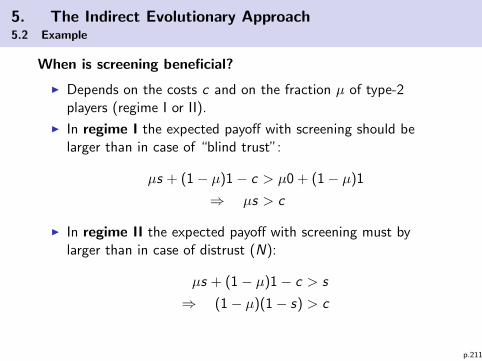
5. The Indirect Evolutionary Approach5.2 Example
When is screening beneficial?
I Depends on the costs c and on the fraction µ of type-2players (regime I or II).
I In regime I the expected payoff with screening should belarger than in case of “blind trust”:
µs + (1− µ)1− c > µ0 + (1− µ)1
⇒ µs > c
I In regime II the expected payoff with screening must bylarger than in case of distrust (N):
µs + (1− µ)1− c > s
⇒ (1− µ)(1− s) > c
p.211
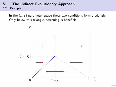
5. The Indirect Evolutionary Approach5.2 Example
In the (µ, c)-parameter space these two conditions form a triangle.Only below this triangle, screening is beneficial.
c
0 µ1− s
(1− s)s
1
p.212

5. The Indirect Evolutionary Approach5.2 Example
I Below the triangle the type of the player is known so that firstplayer can discrimiate like in case 1. As we have seen, type-1players have an advantage, and evolutionary selection will leadto a decreasing µ.
I Above the triangle players will not screen. In this case there isanonymity, and type-2 players have an evolutionary advantage(case 2), i.e. µ will increase.
I Depending on the initial value of µ and the screening costs c,the left side of the triangle represents possible ESS equilibriawith stable mixtures of type-1 and type-2 players.
I Trust and trustworthisness develop in mutual dependency.Agents must be enabled to develop discrimitaion technologiesin order to cooperate conditionally.
p.213

5. The Indirect Evolutionary Approach5.3 The IEA to Reciprocity
Literature:
Berninghaus, S., Korth, C., Napel, S. (2007), Reciprocity – an indirect
evolutionary analysis. Journal of Evolutionary Economics 17, 579-603
I Outcome preference models like Fehr/Schmidt orBolton/Ockenfels, as well as intentionally based models likeRabin or Dufwenberg/Kirchsteiger, and mixed models likeFalk/Fischbacher suffer from ad hoc assumptions aboutpreferences which “explain” behavior.
I Preferences themselves can be explained by an indirectevolutionary amalysis. This is applied to the Falk/Fischbacherapproach of reciprocity in case of the ultimatum game, thedictator game, and a mixed environment of both, called“game of life”.
p.214

5. The Indirect Evolutionary Approach5.3 The IEA to Reciprocity
I The free parameters of the Falk/Fischbacher approach are thereciprocity parameter ρi (for ρi = 0 we have pureself-interest), and the parameter εi which measures the pureconcern about the outcome inequality. The adjustment ofthese free parameters should be explained by an evolutionaryadaption process which is guided by the material success ofthe induced behavior.
I Preferences cannot be conditioned on whether playing anultimatum or dictator game (“game fitting”). Especiallyfairness preferences may vary accross different game settings.
I The evolutionary process should rely on the material outcomein a mixed (multi-game) setting.
p.215

5. The Indirect Evolutionary Approach5.3 The IEA to Reciprocity
I The authors choose the Neutrally Stable Strategy equilibriumconcept (NSS)
(for details see Weibull, J.W. (1995), Evolutionary game theory. MIT
Press.)
I Definition: A strategy profile s∗ is NSS if
u(s∗, s∗) ≥ u(s ′, s∗) ∀s ′ (best reply to itself)
and if u(s∗, s∗) = u(s ′, s∗) then
u(s ′, s ′) ≤ u(s∗, s ′)
p.216

5. The Indirect Evolutionary Approach5.3 The IEA to Reciprocity
Results for th Ultimatum Game:
I It can be seen that the expected material payoffs of i areincreasing with ρi .
I Since the agents have the same material payoff functions, theevolutionary dynamic converges to an identical, significantlypositive level of the reciprocity parameter ρ∗.
I The parameter εi has no effect, so that NSS does not selectfor this parameter.
Results for Dictator Game:
I It can be shown that any strategy in a game with εiρi < 1leads to the same behavior and cannot be distinguished frompurely selfish behavior, and that this is NSS.
p.217

5. The Indirect Evolutionary Approach5.3 The IEA to Reciprocity
Mixed Environment:
I It is λ the probability to play the UG, while 1− λ is theprobability to play the DG.
I NSS implies preferences with ε < 1/ρ (according to the DGNSS), and ρ is a significantly positive reciprocity parameter(according to the UG NSS).
I That is, we can expect strong reciprocity in situaions whereintentionality plays a critical role (e.g. equal split in UG), butno fairness when intentions play no role (e.g. selfishness inDG). Therefore, the different behavior in UG and DG isgenerated by the same preferences.
I This is only partially in line with experimental results. Thelatter show positive proposals also in the DG which can bereconciled with parameter restrictions on ε ≥ ε.
p.218

5. The Indirect Evolutionary Approach5.4 Methodological discussion
I Important step out of the “non-falsifiability trap” becausenon-observable parts of the explanans (“social preferences”)are not assumed ad hoc but explained by a rigorousequilibrium concept which is based on material (observable)payoffs.
I However, since m is “added” to the utility function, thecategorical difference between material outcome and itsvaluation – represented as utility – is not sharp. It must beclear that u(x) are not vNM utilities.
I Even though social and intrinsic motives are permitted, allmethodological and empirical objections against the axiomaticutility approach are still valid. In case of “exploiting the otherplayer’s trust”, it is reasonable to consider that the choice actitself is valued rather than its outcome.
p.219

5. The Indirect Evolutionary Approach5.4 Methodological discussion
I Evolution is a process which selects behavior “from outside”:Individuals die off or do not find sexual partner to replicate theirgenes; firms go bankrupt and leave the market etc.
I Thus, the evolutionary dynamic should not be confused withindividual learning . Individual learning processes are determined bysuccess and failures which depends on the subjective valuations ofoutcomes as described by utility u(x ,m). Learning or choosingpreferences on the basis of existing preferences would imply somelogical problems.
see e.g. Frank, R.H. (1987), If Homo Economicus Could Choose His Own
Utility Function, Would He Want One with a Conscience? American
Economic Review Vol. 77(4), 593-604.
I Hence, the IEA is not an appropriate approach to explain learningbehavior, it is related to a natural selection process “from outside”.
I The approach does not deal with “bounded rationality” since agentsbehave perfectly rational according to their (social) preferences.
p.220

6. Expectations and Fundamental Uncertainty
Outline:
7.1 The Concept of Rational Expectations (RE)
7.2 Empirical and Methodological Problems with RE
7.3 Alternative Expectation Hypotheses
7.4 The Problem of Fundamental Uncertainty
Literature:
(will be given in the subsections)
p.221

6. Expectations and Fundamental Uncertainty6.1 The Concept of Rational Expectations (RE)
Literature:
I Maddock, R., Carter, M. (1982), A Child’s Guide to RationalExpectations. Journal of Economic Literature Vol. 20, 39-51.
I Shaw, G.K. (1987), Rational Expectations. Bulletin ofEconomic Research Vol. 39(3), 187-209.
I Muth, J. (1961), Rational Expectations and the Theory ofPrice Movements. Econometrica Vol. 29, 315-335.
“[Rational Expectations] are essentially the same as thepredictions of the relevant economic theory”(Muth (1961),316).
p.222

6. Expectations and Fundamental Uncertainty6.1 The Concept of Rational Expectations (RE)
A theory which is based on rational individuals has to consider thatindividuals will learn from their errors, they will not rest theirdecisions on systematic errors. If we allow for systematic errorsthen the (ad hoc) assumptions about the errors will drive theresults. Expectations about states, the decisions based onexpectations, and the states resulting from the decisions must beconsistent.
“[...] what must expectations be if actions based onthese expectations are to lead to outcomes that confirmthe expectations?” (Hahn, F. (1982), Money andInflation. Oxford).
p.223

6. Expectations and Fundamental Uncertainty6.1 The Concept of Rational Expectations (RE)
Economic
variables
parameterdistribution
of stochastic
variables
choices expectations
p.224

6. Expectations and Fundamental Uncertainty6.1 The Concept of Rational Expectations (RE)
I The information requirement for RE in a narrow sense areenormous: model structure (the “true” model), parameters,distribution of stochastic variables ⇒ information set Ωt
I The state of the economy is characterized by vector xt .
I Expectations xet+1 induce decisions zt which are transformedvia the causal model f into the state xt+1 = f (zt , ...) which isin average exactly what the agents have excpected:
xet+1 = E [xt+1|Ωt ]
(in average means: up to a neutral stoachstic error)
I This implies that RE are an equilibrium concept: Agents canonly expect equilibria (incl. equilibrium movements).
p.225

6. Expectations and Fundamental Uncertainty6.1 The Concept of Rational Expectations (RE)
Example:
Supply: qst = a + bpetDemand: qdt = c − dpt + εt , εt ∼ N(0, σ2)
The equilibrium price is
qst = qdt
⇒ pt =c − a− bpet + εt
d
Rational expectations: pet = E [pt ]. Because E [εt ] = 0 we have:
pet = E [pt ] =c − a− bE [pt ]
d
⇒ E [pt ] =c − a
d + b
p.226

6. Expectations and Fundamental Uncertainty6.1 The Concept of Rational Expectations (RE)
Some important implications:
I If agents will not make systematic errors when buildingexpectations, policy makers can only implement a credibletime-consistent policy. They have to take into account, thatannouncement and implementation of policy measures will notonly affect the state of the economy (naive policy) but alsothe expectations of the public. The latter will induceadaptions of their plans – which changes the effectiviness ofthe policy measure (Lucas critique).
Lucas, R.E. (1976), Econometric Policy Evaluation: A Critique.
Journal of Monetary Economics (Supplement) Vol.1, 19-46.
I In large dynamic macroeconomic models it would be mucheasier if expectations are calculated on the basis of pastrealized data. RE models, instead, require that they are(computationally) solved for steady states first.
p.227

6. Expectations and Fundamental Uncertainty6.1 The Concept of Rational Expectations (RE)
RE in strategic situations:
I An RE equilibrium requires that agents have consistentexpectations about the expectations of the other players(including expectations about their excpectations.... and soon) – infinite hierachy of beliefs.
⇒ Common Knowledge assumption
I Without any restrictions regarding the prior beliefs almostevery state of a system could be regarded as a RE equilibrium.A proper restriction is the Coomon Prior Assumption.
Aumann, R.J., Dreze, J.H. (2008), Rational Expectations in Games. American
Economic Review 98, 72-86.
p.228
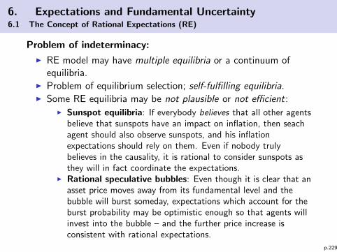
6. Expectations and Fundamental Uncertainty6.1 The Concept of Rational Expectations (RE)
Problem of indeterminacy:
I RE model may have multiple equilibria or a continuum ofequilibria.
I Problem of equilibrium selection; self-fulfilling equilibria.I Some RE equilibria may be not plausible or not efficient:
I Sunspot equilibria: If everybody believes that all other agentsbelieve that sunspots have an impact on inflation, then seachagent should also observe sunspots, and his inflationexpectations should rely on them. Even if nobody trulybelieves in the causality, it is rational to consider sunspots asthey will in fact coordinate the expectations.
I Rational speculative bubbles: Even though it is clear that anasset price moves away from its fundamental level and thebubble will burst someday, expectations which account for theburst probability may be optimistic enough so that agents willinvest into the bubble – and the further price increase isconsistent with rational expectations.
p.229

6. Expectations and Fundamental Uncertainty6.1 The Concept of Rational Expectations (RE)
Rational Expectations in a broader sense:
I Typical situation: asymmetric information – not all agentshave all relevant information which is necessary to computean equilibrium.
I Example: parameter x is not known.
I Which are possible parameter values?⇒ typologization, e.g. x ∈ [0, 5] = X
I Building prior expectations⇒ probability density on X , e.g. x ∼ U[0, 5].
p.230

6. Expectations and Fundamental Uncertainty6.1 The Concept of Rational Expectations (RE)
I Decisions are based on these expectations.They are only ex ante equilibrium decisions.Ex post the agents observe the realized state.
I Agents update their expectations according to Bayes’ Rule⇒ a posteriori expectations. Updated beliefs are consistentwith observed data.
I Under not too restrictive conditions the Bayesian updatingprocess converges to a RE equilibrium.
p.231

6. Expectations and Fundamental Uncertainty6.1 The Concept of Rational Expectations (RE)
Some nobel prizes which are related to RE:
I 2004 – Finn E. Kydland, Edward C. Prescott
“for their contributions to dynamic macroeconomics: the timeconsistency of economic policy and the driving forces behindbusiness cycles.”
I 1995 – Robert E. Lucas Jr.
“for having developed and applied the hypothesis of rationalexpectations, and thereby having transformed macroeconomicanalysis and deepened our understanding of economic policy.”
A collection of important papers in the early stages of the RE approachcan be found in
I Lucas, R.E., Sargent, T.J. (eds.) (1981), Rational Expectations andEconometric Practice, Vol. 1. Minneapolis.
p.232

6. Expectations and Fundamental Uncertainty6.2 Empirical and Methodological Problems with RE
Are RE a behavioral assumption or a modelling strategy?
I RE as a expectation building hypothesis similar to RationalChoice as a decision hypothesis ⇒ problem whether this is aempirically valid positive theory.
I RE as a modelling strategy: restricting expectations to thosewhich are consistent in order to avoid ad hoc assumptions.
I As if approach: single agents may have arbirtraryexpectations, nevertheless an aggregated RE model isconsistent as long as its predictions are in line with the data.
p.233

6. Expectations and Fundamental Uncertainty6.2 Empirical and Methodological Problems with RE
Methodological problems:
I Most important: What is the “true” model?
I A model is by definition an abstraction, what does “true”mean? It is possible that all agents believe in a “wrong”model in a way that beliefs, decicions and realized states areconsistent. From a methodological point of view we can provemodels as false but we cannot prove models as “true”.
Loasby, B.J. (2003), Closed Models and Open Systems. Journal of
Economic Methodology 10(3), 285-306.
I There might be many “observationally equivalent” RE modelswhich differ in their structure but have expectations which areconsistent with the same set of realized data. Which one isthe “true” one?
Beyer, A., Farmer, R. E. (2003), On the Indeterminacy of Determinacy
and Indeterminacy. ECB Working Paper No.277.
p.234

6. Expectations and Fundamental Uncertainty6.2 Empirical and Methodological Problems with RE
I How to account for heterogeneity? If different agents believein different models, then they have to take this fact intoaccount (Common Knowledge assumption). But then, whichone is the “right” one? Do RE rule out any heterogeneity?
I If we doubt about the “truth” of a model and about thequestion whether there is a unique truth, we point to theproblem of fundamental uncertainty (see later section).
Frydman, R., Phelps, E.S. (eds.) (2013), Rethinking Expectations. The Way
Forward for Macroeconomics. Princeton University Press.
p.235

6. Expectations and Fundamental Uncertainty6.2 Empirical and Methodological Problems with RE
I Deterministic chaos: In deterministic models, RE are thesame as perfect foresight. Nonlinear chaotic systems, however,have the property that a perfect (long run) prediction ispossible only if parameters and initial concitions are knownwith infinite accuracy since the produced time-series are“chaotic” (look like stochastic). Due to physical and logicallimits, accuracy is limited. Then the prediction error increasesin time even though the system is deterministic. Here, theconcept of RE seems not to make (logical) sense.
Lorenz, H.-W. (1993), Nonlinear Dynamical Economics and Chaotic
Motion, 2nd ed. Berlin et al.: Springer.
p.236

6. Expectations and Fundamental Uncertainty6.2 Empirical and Methodological Problems with RE
I Building RE may be suboptimal/inefficient:
I Benassy, J.-P. (1992), Are Rational Expectations ReallyRational? Economics Letters Vol.39, 49-54.
I Stegman, T.R. (1985), On the Rationality of RationalExpectations Hypothesis. Australian Economic Papers Vol.24, 350-355.
I Woodford, M. (2012), Prospect Theory as Efficient PerceptualDistortion. American Economic Review 102(3), 41-46.
I Kirman, A. (2014), Is It Rational to Have RationalExpectations? Mind and Society 13(1), 29-48
⇒ Why should people build expectations and learn from data ina consistent way in cases where other expectation rules inducemore successful behavior?
p.237

6. Expectations and Fundamental Uncertainty6.2 Empirical and Methodological Problems with RE
Empirical problems:
There are many experimental and field studies which disprove REas an empirically valid hypothesis, examples:
* Lovell, M.C. (1986), Tests of Rational Expectations Hypothesis.American Economic Review Vol. 76, 110-124.
I Brennscheidt, G. (1993), Predictive Behavior. An Experimental Study.Berlin et al.
I Kahneman, D., Slovic, P., Tversky, A. (eds.) (1982), Judgement underUnceretainty: Heuristics and Biases. Cambridge.
I Kagel, J., Roth A.E. (eds.) (1995), Handbook of ExperimentalEconomics. Princeton.
Wikipedia: “List of cognitive biases”
p.238

6. Expectations and Fundamental Uncertainty6.2 Empirical and Methodological Problems with RE
“Confidence is what you have before you understand the problem.”(Woody Allen)
Examples:
a) Overweighting of small probabilities, underweighting of largeprobabilities (S-shaped weighting function)
b) People are overconfident to their estimations/expectations.Consequences (e.g.): investment into too risky projects,inefficient insurance against risk
p.239

6. Expectations and Fundamental Uncertainty6.2 Empirical and Methodological Problems with RE
c) Problems with Bayesian updating:
Kahneman and Tversky (1972): A cab had an traffic accident.There are two cab companies, the Green and the Blue, where85% of the cabs in the city are green and 15% are blue. Awitness identified the cab as blue. The court tested thereliablity of the witness and found that the witness correctlyidentifies the color 80% of the time and failed 20% of thetime. What is the probability that the cab was blue?Median answer: 0.8 (underweighting of base rates)Correct answer according to Bayes’ rule:
0.15 · 0.80.15 · 0.8 + 0.85 · 0.2
≈ 0.414
p.240

6. Expectations and Fundamental Uncertainty6.2 Empirical and Methodological Problems with RE
Another example: The “goat problem”
I In an american quiz show the candidate is offered three doors.Behind one door there is a precious prize, behind the otherdoors are “goats” (another word for blank). The quizmasterknows where the prize is. After the candidate has decided forone door, the quizmaster announces that he will relieve thefinal decision by opening one of the remaining doors with agoat. Should the candidate now correct his first choice andchoose the other (remaining) door?
I See Wikipedia article on the “Goat problem” (or “Monty Hallproblem”)
I See also: El-Gamal, M.A., Grether, D.M. (1995), Are PeopleBayesian? Uncovering Behavioral Strategies. Journal of theAmerican Statistical Association Vol. 90, 1137-1145.
p.241

6. Expectations and Fundamental Uncertainty6.2 Empirical and Methodological Problems with RE
d) Representativeness:
“Steve is intelligent, curious and introvert. Hecannot get along with other people. Whichprofession Steve will choose with the highestprobability? (A) farmer, (B) salesman, (C)physicist.”
Most people choose “physicist” as this appears mostrepresentative (according to a stereotype of a physicist),although the a priori probability to become a salemsman isdrastically larger.
p.242

6. Expectations and Fundamental Uncertainty6.2 Empirical and Methodological Problems with RE
e) Misspecification of probability
I Throwing a coin. Consider the sequence 0-0-1-0-0-0-1. Is it a“fair” coin? (judgement is based on a far to small sample,relative frequency is then not a good predictor for probability)
I Given two results of the German lottery “7 aus 49”:1-2-3-4-5-6-7 and 5-11-17-25-31-39-40. Which one is moreprobable?
I Gambler’s fallacy: history of stochastic events “matters”.
f) ... any many others.
Some of these problems can be alleviated if there are sufficient(e.g. monetary) incentives for the statistically correct answer,if persons have more time for making judgements, and ifjudgements are made by groups instead of single persons (but:“group thinking” effect).
p.243

6. Expectations and Fundamental Uncertainty6.3 Alternative Expectation Hypotheses
I RE require information about the model, its parameters anddistributions of stochastic variables (and about theexpectations of other players).
I Alternative expectation hypothesis requires much lessinformation – at the price that they are systematically biased.They are based on past realizations of variables.
p.244

6. Expectations and Fundamental Uncertainty6.3 Alternative Expectation Hypotheses
a) Static expectations:
xet+1 = xt
Agent does not expect a systematic change of the previousrealization.
b) Adaptive expectations:
xet+1 = xet + λ(xt − xet ), λ ∈ (0, 1)
The former expectations are partially corrected by λ times theobserved expectation error in the last period. Note that withλ = 1 we have static expectations. The factor λ may be afunction (λ changes in time).
p.245

6. Expectations and Fundamental Uncertainty6.3 Alternative Expectation Hypotheses
c) Extrapolative expectations:
xet+1 =t∑
i=0
aixi with∑i
ai = 1
Expectations are a linear combination of past realizations (e.g.like trend extrapolation). The weighting parameters can bedetermined e.g. by least squared learning. The weights mightchange in time.
I Note that extrapolative expectations have to be “initialized”when there are no prior realizations
I An agent with sophisticated extrapolative expectations is thenlike an econometrican who applies a VAR model.
Empirical/experimental evidence for adaptive expectations(see. e.g. Brennscheidt (1993))
p.246

6. Expectations and Fundamental Uncertainty6.3 Alternative Expectation Hypotheses
Question: Does updating boundedly rational expectations such likeadaptive expectations converge to RE equilibrium?
I Under certain conditions: Yes!
I Moreover, they can be a device to select RE equilibria in caseof multiple equilibria.
I See: Evans/Honkapohja (1994), Marcet/Sargent (1989),Marimon/McGrattan (1993), Sargent (1993),
Kirman, A., Salmon, M. (eds.) (1993), Learning andRationality in Economics. Oxford.
p.247

6. Expectations and Fundamental Uncertainty6.4 The Problem of Fundamental Uncertainty
“There are known knowns; there are things we know we know. Wealso know there are known unknowns; that is to say, we know thereare some things we do not know. But there are also unknownunknowns—the ones we don’t know we don’t know.”(Donald Rumsfeld, former US Secretary of Defense)
Literature:I Dequech, D. (2000b), Fundamental Uncertainty and Ambiguity. Eastern
Economic Journal 26(1), 41-60.
I Dequech, David (2011). Uncertainty: A Typology and Refinements ofExisting Concepts. Journal of Economic Issues 45 (3), 621-640.
I Dow, S. (2016), Uncertainty: A Diagrammatic Treatment. Economics:The Open-Access, Open-Assessment E-Journal, 10 (2016-3): 1-25.
I Hoogduin, L. (1987), On the Difference Between the Keynesian,Knightian and the “Classical” Analysis of Uncertainty and theDevelopment of a More General Monetary Theory. De Economist 135(1),52-65.
I Ormerod, P. (2015), The Economics of Radical Uncertainty. Economics:The Open-Access, Open-Assessment E-Journal, 9 (2015-41): 1-20.
p.248

6. Expectations and Fundamental Uncertainty6.4 The Problem of Fundamental Uncertainty
I Uncertainty about the realization of a stochastic variable in anotherwise well-specified model⇒ risk in a narrow sense
I Uncertainty about parameters or functions⇒ Bayesian approach⇒ risk in a broader sense/uncertainty
I What if the decision problem, the perception of the world isnot well specified, vague, imprecise? If there is lack ofconclusive knowledge? Although is is always possible to“construct” a closed model and to solve it with Bayesianrationality, this seems to be very arbitrary and doubtful.⇒ fundamental uncertainty
p.249

6. Expectations and Fundamental Uncertainty6.4 The Problem of Fundamental Uncertainty
I Example: the “Turkey” problem.
I Knowledge which is required to make any probabilityjudgements, is not available or it is inconclusive:
I Knight, F. (1921), Uncertainty and Profit, University ofChicago Press.
I Keynes, J.M. (1921), A Treatise on Probability. MacMillan.
I Reasons:I Structural change of the underlying causal relationships of the
decision environment (note, that economy evolves in historicaltime!)
I Creativity (new technologies, opportunities, institutions,...)⇒ Knowledge about decision environment is always incomplete
and vague. Small pieces of information might drasticallychange the expectations.
p.250

6. Expectations and Fundamental Uncertainty6.4 The Problem of Fundamental Uncertainty
How could a “rational” agent act in a fundamentally uncertainworld?
Keynes:
I Liquidity preference (hording) as a response to fundamentaluncertainty because liquidity can be transformed in everythingif the economy evolves in an unperceived way.
I “Animal spritis” of investors.
p.251

6. Expectations and Fundamental Uncertainty6.4 The Problem of Fundamental Uncertainty
Decision Theory:
I Non-additive probabilities:
Gilboa, I. (1987), Expected Utility Theory with Purely Subjective
Non-additive Probabilities. Journal of Mathematical Economics 16,
65-88.
I Multiple priors:
Gilboa, I., Schmeidler, D. (1989), Maxmin expected utility with
non-unique prior. Journal of Mathematical Economics 18(2),
141-153.
I Limited trust to the subjective prior beliefsI What are the choice preferences for different priors?I Which choice is “best for diffrent priors”?I Which choice is best for the worst possible prior?
p.252

6. Expectations and Fundamental Uncertainty6.4 The Problem of Fundamental Uncertainty
I Ambiguity:I Aversion against the fact that something depends on
subjective assignments.I Missing knowledge whether model X (alternatives, states,
outcomes, assigned probabilities) is valid.I Limted trust to model X ⇒ constructing multiple models
X1,X2, ... and exploring the best choices in different models.I Putting more weight on models which are less reliant on
subjective priors.
Camerer, C. F., Weber, M. (1992), Recent development in modelingpreferences: Uncertainty and ambiguity. Journal of Risk and Uncertainty5, 325-370.
Ghirardato, P., Maccheroni, F., Marinacci, M. (2004), Differentiatingambiguity and ambiguity attitude. Journal of Economic Theory 118(2),133-173.
Ghirardato, P., Marinacci, M. (2002), Ambiguity made precise: A
comparative foundation. Journal of Economic Theory 102(2), 251-289.
p.253

6. Expectations and Fundamental Uncertainty6.4 The Problem of Fundamental Uncertainty
Application of Ambiguity Approach: Ellsberg Paradoxon
I Urn with 50 blue balls and 100 balls with an unknownproportion of red and green balls.
I Choice problem A: L1= win with blue, L2= win with red.
I Choice problem B: L3= win with (blue and green), L4= winwith (red and green).
I Typical result: L1 L2 and L4 L3 which is a violation ofSTP (“green” is the sure thing)
I In problem A, the winning probability of L1 is clear (1/3),while in case of L2 it is only “in average” 1/3. In problem B,the probability of L3 is only “in average” 2/3 while that of L4is 2/3 for sure.
I Ambiguity means here that you don’t trust the “average”calculation because it might turn out to be wrong ex post.People seek to avoid such uncertainty/ambiguiity.
p.254

6. Expectations and Fundamental Uncertainty6.4 The Problem of Fundamental Uncertainty
I Fuzzy Set Theory:
Mathematical but non-probabilistic concept; describing vagueknowledge (e.g. about parameters) with “fuzzy sets”; a stateof a variable is “more possible” rather than “more likely”.
Cherubini, U. (1997), Fuzzy Measures and Asset Prices: Accounting
for Information Ambiguity. Applied Mathematical Finance 4,
135-149.
p.255

6. Expectations and Fundamental Uncertainty6.4 The Problem of Fundamental Uncertainty
Discussion:
I Expectations plus limited trust/confidence in theseexpectations ⇒ ambiguities and ambiguity preferences areoften accepted as an appropriate formalization of Knightian orKeynesian fundamental uncertainty.
I However, ambiguity is not Fundamental or Keynesianuncertainty. Ambiguity requires closed set of possibleoutcomes and possible events. Recall “things you don’t knowthat you don’t know them” ⇒ closed sets are not a suitablerepresenation as a matter of principle.
I “Optimal” decisions when facing ambiguity depend cruciallyon ambiguity preferences ⇒ non-observable explanans,tendency to non-falsifiability when “explaining” consistentbehavior in vague situations.
p.256

6. Expectations and Fundamental Uncertainty6.4 The Problem of Fundamental Uncertainty
Remarks:
I Even if not following non-expected utility theory (e.g.ambiguity approach) one has to clarify what “rational”behavior in a FU world means ⇒ simple rules?
I Back to Keynes’ liquidity preference theory: FU about theunderlying process which drives the returns (expected valuesand covariances) of the investment opportunities⇒ how to structure a portfolio under FU?⇒ the more FU, the more riskless money the investor holds,the higher the interest rate must be in order to waive forliquidity.
p.257

7. Rule-governed Behavior and Rule Rationality
Outline:
7.1 Rule-goverend Behavior
7.1.1 “Fast and Frugal Heuristics”7.1.2 Case-based decision making7.1.3 Information processing errors and rule-binding7.1.4 Melioration7.1.5 From Maximizing to Satisficing
7.2 Rule Rationality
7.2.1 Rule Rationality and Act Rationality7.2.2 Concept of Equilibrium Rule Profiles7.2.3 Example
Literature: (will be given in the subsections)
p.258

7. Rule-governed Behavior and Rule Rationality7.1 Rule-goverend Behavior
I Information processing and decision making as an algorithm.
I Approach by Lipman, B. (1995), Information Processing andBounded Rationality: a Survey. Canadian Journal ofEconomics 28, 42-67.
I Possible states of the world: Z ; choice set: AI Selecting information and mental representation of the world:ξ : Z → Ω.
I Inference process; generating beliefs: β : Ω→ ∆.I Selecting choices: α : ∆→ AI Transformation of ”‘inputs”’ (world = stimuli) to ”‘outputs”’
(choices) is characterized as a “rule”: f : Z → A withf (z) = α(β(ξ(z))).
I Call f a rule (e.g. heuristic).
p.259

7. Rule-governed Behavior and Rule Rationality7.1 Rule-goverend Behavior7.1.1 “Fast and Frugal Heuristics”
I How do humans process information, make statisticalinferences, build expectations, and come to decisions?
I Cognitive Psychology: “Fast and frugal heuristics”:
I Gigerenzer, G., Selten, R. (2001), Rethinking Bounded Rationality.In: Gigerenzer, G., Selten, R. (eds.), Bounded Rationality. TheAdaptive Toolbox. Cambridge Mass./London.
I Gigerenzer, G., Brighton, H. (2011), Homo Heuristics: Why BiasedMinds Make Better Inferences. In: Gigerenzer, G., Hertwig, R.,Pachur, T. (eds.), Heuristics: The Foundations of AdaptiveBehavior. Oxford Univrsity Press.
I Gigerenzer, G., Todd, P. M. and The ABC Research Group (1999),Simple Heuristics that Make us Smart. Oxford University Press.
I Reimer, T., Hoffrage, U. (2006), The Ecological Rationality ofSimple Group Heuristics: Effects of Group Member Strategies onDecision Accuracy. Theory and Decision 60(4), 403-438
p.260

7. Rule-governed Behavior and Rule Rationality7.1 Rule-goverend Behavior7.1.1 “Fast and Frugal Heuristics”
Basic ideas:
I Cognitive structures and processes have beenevolutionary adapted to guide behavior successfully in acomplex dynamic environment.
I Selective perception, reducing complexity, focusing on fewrelevant informations – instead of processing all availableinformation
I Using simple but effective decision heuristics – instead ofsolving complex optimization problems
I Strategic role of emotions in decision making.
I Commitment to social/moral norms, role of groups
I Many behavioral relevant issues do not come to awareness ofthe decison maker.
p.261

7. Rule-governed Behavior and Rule Rationality7.1 Rule-goverend Behavior7.1.1 “Fast and Frugal Heuristics”
Heuristics do not lead to “optimal” outcomes but:
I Faster than complex deliberation processes.
I Require less information.
I Eventually robust against information processing errors.
I Applicable even if knowledge is insufficient to compute“optimal” outcomes.
I Induce predictable behavior which facilitates strategicinteraction.
⇒ lead in average to successful behavior.
p.262

7. Rule-governed Behavior and Rule Rationality7.1 Rule-goverend Behavior7.1.1 “Fast and Frugal Heuristics”
I The view of rule-governed or heuristic behavior is seen as anexpression of “bounded rationality” .
I Bounded rationality is seen not as a generalization but as anopposing paradigm to rational choice
(in our terms: f is a rule, algorithm, behavioral program, not
necessarily the result of a caclulus):
I Berg, N., Gigerenzer, G. (2010), As-If Behavioral Economics:Neoclassical Economics in Disguise? History of Economic Ideas18(1), 133-165
I Selten, R. (1990), Bounded Rationality. Journal ofInstitutional and Theoretical Economics Vol. 146, 649-658.
I In the following we discuss few economic approaches torule-governed behavior as well as “Satisficing” as analternative choice criterion.
p.263

7. Rule-governed Behavior and Rule Rationality7.1 Rule-goverend Behavior7.1.2 Case-based decision making
I Gilboa, I., Schmeidler, D. (1995), Case-Based Decision Theory.Quarterly Journal of Economics Vol. 110, 605-639.
I Gilboa, I., Schmeidler, D. (2001), A theory of case-based decisions.Cambridge. (online version available)
I Looking for situations which are “similar” to other situationsaccording to certain criteria, so that the experience in similarsituations can be applied to the current problem.
⇒ Similar situations will create similar decisions.
I Since CBDT is based on algorithms, it is also applicable tocomputerized data exploration (computer reasoning).
I Since it is an inductive method (case-based reasoning, CBR),the conclusions drawn from very few experiences (“anecdotalevidence”) may be questionable.
p.264

7. Rule-governed Behavior and Rule Rationality7.1 Rule-goverend Behavior7.1.2 Case-based decision making
Examples:
I A lawyer looks for legal precedential cases in order to make ajudgement in a new particular case.
I When repairing a car or making a medical diagnosis theexperiences of “similar” cases in the past (similar symptoms)trigger the behavior of the car mechanic or physician.
I Parents respond to sudden screaming of their child morerelaxed if they have the experience with elder siblings thatchilds sometimes only cry in order to get more attention.
I In general: experienced persons behave differently thannewbies due to a knowledge base of many “similarexperiences” in the past.
p.265

7. Rule-governed Behavior and Rule Rationality7.1 Rule-goverend Behavior7.1.2 Case-based decision making
I CBDT emphasizes the procedural character of choice.
I Main question: Which choices have been proven to besuccessful in the past in case of similar decision problems?
I Detecting “similarities” and “differences” plays an importantrole in human decision making and thus in behavioral decisiontheories.
⇒ Necessary criterion for “similar”: The more differentiatedinformation is used, the less cases will be regarded to be“similar”. Similarity increases with reduction of complexity.
p.266

7. Rule-governed Behavior and Rule Rationality7.1 Rule-goverend Behavior7.1.2 Case-based decision making
Example: (for focusing similarities)
Kahnemann, D., Tversky, A. (1979), Prospect Theory: an analysis of decision
under risk. Econometrica 47, 263-291.
Lottery choice A:
L3 = (4000; 0.2), L4 = (3000; 0.25)
Lottery choice B:
L1 = (4000; 0.8), L2 = (3000; 1.0)
(The payoffs for the second case with complementary probabilityare zero). Typical result in experiments: L3 and L2. This violatesSTP because L3 and L4 could be decomposed as:
L3 = 0.25L1 + 0.75 · 0, L4 = 0.25L2 + 0.75 · 0
p.267

7. Rule-governed Behavior and Rule Rationality7.1 Rule-goverend Behavior7.1.2 Case-based decision making
Possible explanation:
I For L3, L4 agents are aware that the payoffs are verydifferent while the probabilities are very “similar”. These smalldifferences are neglected.
I For L1, L2 the payoffs and the probabilities are different(not similar). Agents are aware of the trade-off and the riskattitude is more prominent for decision making.
I The construction of sets of “similar” problems depend on thepresentation/framing: If lotteries L3, L4 are presented asdecomposed lotteries (see above), then the “sure thing” worksas a similarity, so that the decision will be analogue as in caseof L1, L2.
p.268

7. Rule-governed Behavior and Rule Rationality7.1 Rule-goverend Behavior7.1.2 Case-based decision making
Sketch of the Gilboa/Schmeidler approach:
Set of problems PSet of choices ASet of results RSet of cases C = P × A× RMemory M ⊆ C of past experiences
Every single case is a triple (p, a, r).
p.269

7. Rule-governed Behavior and Rule Rationality7.1 Rule-goverend Behavior7.1.2 Case-based decision making
I What means: two problems are “similar”? Depends on thedecision maker’s perception and has to be clarified for eachspecific decision making environment.
I In general we have a similarity function
s : P2 → [0, 1]
I Standard utility function for consequences
u : R → R
p.270

7. Rule-governed Behavior and Rule Rationality7.1 Rule-goverend Behavior7.1.2 Case-based decision making
I At every timepoint the decision maker has the experience M(perhaps limited by cognitive constraints).
I If a new problem p ∈ P occurs, the agent assess the similarityto other problems q ∈ P he solved in the past: s(p, q).
I Choosing an action which has been proven to be mostsuccessful in similar cases in the past:
maxa
U(a) =∑
(q,a,r)∈M
s(p, q)u(r)
I Possible trade-off between high values of u and s.
p.271

7. Rule-governed Behavior and Rule Rationality7.1 Rule-goverend Behavior7.1.2 Case-based decision making
Problems:
I Does not work well with small M (“anecdotal evidence”).
I Searching for better choices requires some experimentation.
I In not too complex situations, agents are able to make moresophisticated forward-looking deliberations.
I Construction of similarity function s is the crucial point –desevres theoretical explanation.
But:
I Psychologically relevant; (partially) good description of humanbehavior (inductivistic generation of pre-scientific conjecturesabout their environment).
I Powerful tool in machine-learning and artificial intelligence.
p.272

7. Rule-governed Behavior and Rule Rationality7.1 Rule-goverend Behavior7.1.3 Information processing errors and rule-binding
I Heiner, R. (1983), The origin of predictable behavior. AmericanEconomic Review Vol. 73, 560-595.
I Heiner, R. (1988a), The necessity of imperfect decisions. Journal ofEconomic Behavior and Organisation Vol. 10, 29-55.
I Heiner, R. (1988b), The necessity of delaying economic adjustment.Journal of Economic Behavior and Organisation Vol. 10, 255-286.
I Up to now we have assumed that agents use only limitedinformation = a reduced model of the environment.
I Questions: How to explain that we observe specific types ofcomplexity reduction and not others? How and why do agentsmake their decisions, based on these reduced representationsof the world?
p.273

7. Rule-governed Behavior and Rule Rationality7.1 Rule-goverend Behavior7.1.3 Information processing errors and rule-binding
The approach by Heiner:
I Considering errors in perceiving and processing informationsas well as in deriving optimal choices.
I Errors prevent from optimal decision behavior. Agent shouldrespond to the fact that there are possible errors, i.e. decisionshould be made in a “robust” way.
I The way, how complexity is reduced and informations areignored, as well as the way how decisions are made can beexplained by reasonable mechanisms which control the impactof errors.
p.274

7. Rule-governed Behavior and Rule Rationality7.1 Rule-goverend Behavior7.1.3 Information processing errors and rule-binding
”‘The reason [for behavioral regularities] is that decisionerrors create potential benefits from controlling themsuccessfully. Such errors thereby produce systematicincentives towards controlling decisions with rules andprocedures that discipline behavior into relatively morepredictable patterns than would otherwise result if therewere no decision errors [...]. Consequentely, analyzing theeffects of decision errors become a powerful newexplanatory source for predicting behavior [...].”’(Heiner 1988a, S.40)
p.275

7. Rule-governed Behavior and Rule Rationality7.1 Rule-goverend Behavior7.1.3 Information processing errors and rule-binding
I There are no structural assumptions about the error (thiswould “explain” nothing).
I Deriving criteria for “robustness” of information processingand decision making. The performance of the behavioral rulef is maximized, considering errors.
I The agent does not need to be able to solve this performancemaximization calculus. It is sufficient to assume that he has“learned” the behavioral pattern.
I The idea is that trying to behave according to EUT inpresence of errors will not only have a poor performance butwill also not lead to stable behavioral patterns. In afluctuating envornment, rational decision behavior would bemore volatile than observed. Behavioral patterns which arerobust against errors create more regularity in behavior.
p.276
7. Rule-governed Behavior and Rule Rationality7.1 Rule-goverend Behavior7.1.3 Information processing errors and rule-binding
Consequences:
I Choice alternatives which are optimal only in rarely occuringsituations, will not be considered. Choice alternatives whichare optimal but only slightly better than other alternatives fora subset of Z , but have a significantly worse performance forother subsets, will not be considered.
I Additional informations may improve decision quality but alsoincrease the risk of additional (performance reducing) errors.Thus, not all available informations are used, but more thanthe agent is able to process correctly.
I The agent will not respond fully and immediately to changesin the informations. There is a rationale for delayed andpartial adjustment.
p.277

7. Rule-governed Behavior and Rule Rationality7.1 Rule-goverend Behavior7.1.3 Information processing errors and rule-binding
A more formal approach:
I Heiner’s formalization follows a very “unorthodox style” Thismight explain why the appealing argument had only limitedimpact on further economic research.
I Possible environmental states: Z .For each state, a certain choice would be optimal.
I The set of perceived signals about the state: X
I Choice set: A
I Decision rule: B : X → A where B∗ denotes the optimalchoice.
I Let X ∗a be the set of signals which indicate that decisiona ∈ A is optimal.
p.278

7. Rule-governed Behavior and Rule Rationality7.1 Rule-goverend Behavior7.1.3 Information processing errors and rule-binding
Incentive to eliminate choice alternatives (“rule binding”):
1. Are the perceived signals x about the environmental statereliable? Or is the reliability limited due to perception errors?
rXa = p(x ∈ X ∗a |Z ∗a ), wXa = p(x ∈ X ∗a |Z − Z ∗a )
Measure for the reliability of perceived information which indicatethat a is the optimal choice:
ρXa =rXawXa
Therefore it is ρXA →∞ for perfect reliability, i.e. rXa → 1. Thereliability is minimal for rXa = wX
a = 0.5 and therefore ρXa = 1 (incase of wX
a > 0.5 the signal would be a good counter indicator...).
p.279

7. Rule-governed Behavior and Rule Rationality7.1 Rule-goverend Behavior7.1.3 Information processing errors and rule-binding
2. Reliability of information processing by the agent. How reliableis an agent with a decision rule B to choose the optimal decision aif the perceived signal X ∗a indicates this?
rBa = p(a ∈ B(x)|X ∗a ) (correct choice of a)
wBa = p(a ∈ B(x)|X − X ∗a ) (incorrect choice of a)
A reliability measure for the agent’s competence to make properdecisions:
ρBa =rBawBa
For a perfect agent it is wBa → 0 and therefore ρBa →∞. Perfect
incompetence means erratic behavior, implying rBa = wBa = 0.5
and henceforth ρBa = 1.
p.280

7. Rule-governed Behavior and Rule Rationality7.1 Rule-goverend Behavior7.1.3 Information processing errors and rule-binding
3. Joint relability: How probable is it that an optimal choice a isselected if a is indeed optimal for a given environmental state?
rXBa = p(a ∈ B(x)|Z ∗a )
wXBa = p(a ∈ B(x)|Z − Z ∗a )
Heiner shows that for all a ∈ A it holds true:
ρXBa =rXBa
wXBa
=rXa (ρBa − 1) + 1
wXa (ρBa − 1) + 1
I In case of extreme unreliable perceived signals, ρXa = 1, also thedecision are extremly unreliable: ρXBa = 1 – irrepective of thecompetence of the agent.
I In case of perfectly reliable signals, the joint reliability does onlydepend on the competence of the agent: ρXBa → ρBa .
p.281

7. Rule-governed Behavior and Rule Rationality7.1 Rule-goverend Behavior7.1.3 Information processing errors and rule-binding
Should the agent consider a choice alternative a, or shouldhe eliminate it from the choice set (called “rule binding”)?
I A false = imperfect decision belongs to the set A− a forthe case that the signal is x ∈ X ∗a (a is the optimal decision).
I The additional benefit that a could be chosen if the signal X ∗ais perceived, compared to the second best alternative whichwould be chosen if a is not any longer in the choice set, isgiven by:
ga = u(a|X ∗a )− u(A− a|X ∗a )
I The additional benefit from eliminating a from the choice setis determined by the fact that a could not chosen by mistakewhen the signal does not indicate a to be optimal:
la = u(A− a|X − X ∗a )− u(a|X − X ∗a )
where u is the utility function.p.282

7. Rule-governed Behavior and Rule Rationality7.1 Rule-goverend Behavior7.1.3 Information processing errors and rule-binding
I Now let πa the exogenously given probability of perceivingsignal X ∗a . Then it is beneficial to have a in the choice set A if
rBa · ga · πa > wBa · la · (1− πa)
I Rearranging gives
ρBa >laga
1− πaπa
≡ Ta
with Ta as a tolerance level for the agent’s reliability ofinformation processing.
I For a perfect agent we have ρBa →∞, so that every tolerancelevel will be exceeded.
I The less competent the agent is, the more choice alternativesshould not be considered but eliminated from the choice set!
p.283

7. Rule-governed Behavior and Rule Rationality7.1 Rule-goverend Behavior7.1.3 Information processing errors and rule-binding
Optimal information perception – optimal ignorance:
Should an agent process more information than he is able toprocess correctly? Should an agent ignore available information?
Assumptions:
I The set of perceived signals X can have different size or theinformation can be differently rich structured. Let z be ameasure of the size (or complexity level) of information.
I The larger or more differentiated the information set, themore reliable is the resulting signal that choice a is optimal:
∂rXa (z)
∂z> 0,
∂wXa (z)
∂z< 0
and ρXa →∞ for z →∞.
p.284

7. Rule-governed Behavior and Rule Rationality7.1 Rule-goverend Behavior7.1.3 Information processing errors and rule-binding
I We assume that an agent can process information reliably upto a level z∗. For z > z∗ he makes errors due to cognitivelimitations.
I For all z ≤ z∗ we assume
ρBa (z) =∞, ∂ρBa (z)
∂z= 0
I But for all z > z∗ it is
∂ρBa (z)
∂z< 0
I This has consequences for the joint reliability.
p.285

7. Rule-governed Behavior and Rule Rationality7.1 Rule-goverend Behavior7.1.3 Information processing errors and rule-binding
ρXBa (z)
ρXa (z)
ρXBa = ρXa
for perfect agents
ρXa (z∗)
perfectdecisionzone
imperfectdecisionzone
p.286

7. Rule-governed Behavior and Rule Rationality7.1 Rule-goverend Behavior7.1.3 Information processing errors and rule-binding
With some given technical assumptions, Heiner shows that thefollowing holds true:
I There exists an incentive to move into the ”‘imperfectdecision zone”’, that is: to perceive more information thancan be perfectly processed. In other words: There is anincentive/necessity to make imperfect decisions.
I There exists an incentive to ignore information, because for asufficiently large z the reliability of processing informationsuffers more than the agent gains from increased reliability ofthe signal itself. This is a rationale for complexity reduction orpartial ignorance of information.
p.287

7. Rule-governed Behavior and Rule Rationality7.1 Rule-goverend Behavior7.1.3 Information processing errors and rule-binding
Delayed adaption to changing environments:
I In a more dynamic perspective, the information which canreliably processed in a certain time interval (information flow)is limited.
I Assumption: The shorter the time interval, the larger are theprocessing errors for a given amount of information.
I If a new information occurs (environment has changed), wehave two effects:
I The former decision is in general not optimal any longer. Theagent faces losses in case of non-adaption to the newinformation.
I Processing the new information creates errors which mightinduce decision errors when adapting to the new situation.The agent may face losses in case of (false) adaption.
p.288

7. Rule-governed Behavior and Rule Rationality7.1 Rule-goverend Behavior7.1.3 Information processing errors and rule-binding
I The shorter the time interval is before the agent responds, thelarger is the information processing error, but the lower arethe losses from keeping a non-optimal decision.
I The longer the time interval is before the agent responds, thesmaller is the information processing error, but the higher arethe losses from keeping a non-optimal decision.
I Heiner shows in terms of reaction rates that the optimalreaction rate goes to zero as the time interval goes to zero. Inother words: It is optimal to have some delay in adapting toenvironmental changes.
I In changing/fluctuating environments, the agents will respondslowly and partially. If agents’ decision behavior influences theenvironment, this creates more regularity and stability thancould be expected from rational choice theory.
p.289

7. Rule-governed Behavior and Rule Rationality7.1 Rule-goverend Behavior7.1.4 Melioration
I Herrnstein, R.J., Prelec, D. (1991), Melioration: A Theory ofDistributed Choice. Journal of Economic Perspecives Vol. 5,137-156.
I Model of boundedly rational consumer decisions, based onpsychology and empirical observations.
I Dynamic behavior in case of repeated choice situations:Dynamic allocation of the consumer’s budget on alternativegoods (distributed choice); effects of experiences and learning.
p.290

7. Rule-governed Behavior and Rule Rationality7.1 Rule-goverend Behavior7.1.4 Melioration
Example:
I Assume that there are only two meals in the mensa: sausageand pizza. There is a fixed budget which has to be allocatedfor subsequent days. To avoid further complications, weassume that both meals have the same price.
I Assume decreasing marginal utility. A rational agent wouldchoose a 5-day allocation which maximizes the total utility(note that we have no discounting). In optimum the marginalutility of both meals must be equal (or almost equal since wehave a discrete choice problem).
I This requires that the agent knows ex ante the marginaleffects of eating sausage and pizza (= before he has eaten it).Or he must have a clear picture ex ante about the utility of allpossible 5-day allocations. This is not very reasonable.
p.291

7. Rule-governed Behavior and Rule Rationality7.1 Rule-goverend Behavior7.1.4 Melioration
I In case of melioration the agents collects experiences wheneating sausage and pizza. He will make consecutive decisionsaccording to the experienced average utility.
I Due to this melioration process the average utility of bothmeals will be equalized – instead of the marginal utility.Henceforth, allocation will not be optimal.
I The approach emphasizes the process of decision making ;decisions are made with low information requirements;decisions are based on experiences.
p.292

7. Rule-governed Behavior and Rule Rationality7.1 Rule-goverend Behavior7.1.4 Melioration
Formal representation:
I Number of alternatives i = 1, ...n (here: n = 2)
I Share of alternative i of the allocated budget: xi ∈ [0, 1]
I Allocation x = (x1, ..., xn) with∑
xi = 1.
I Utility function u(x)
I Value accounting function vi (x) with∑i
xivi (x) = u(x)
which could be interpreted as the average utility contributionof alternative i .
I Observe, that several (xi , vi )-combinations could becompatible with one utility function u.
p.293
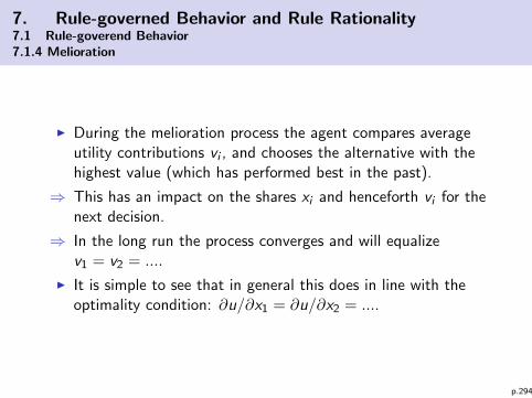
7. Rule-governed Behavior and Rule Rationality7.1 Rule-goverend Behavior7.1.4 Melioration
I During the melioration process the agent compares averageutility contributions vi , and chooses the alternative with thehighest value (which has performed best in the past).
⇒ This has an impact on the shares xi and henceforth vi for thenext decision.
⇒ In the long run the process converges and will equalizev1 = v2 = ....
I It is simple to see that in general this does in line with theoptimality condition: ∂u/∂x1 = ∂u/∂x2 = ....
p.294

7. Rule-governed Behavior and Rule Rationality7.1 Rule-goverend Behavior7.1.4 Melioration
Numerical example:
vpizza = 4x
vsausage = 2− x
u(x) = x · vsausage + (1− x) · vpizza= 6x − 5x2
with x as the share of sausage. Utility is concave in share x whichis compatible with standard utility function of the consumedquantities of sausages and pizza.
From optimality condition ∂u/∂x = 0 and the meliorationcondition vpizza = vsausage it follows:
xopt =3
5, xmel =
2
5
p.295
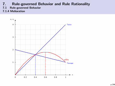
7. Rule-governed Behavior and Rule Rationality7.1 Rule-goverend Behavior7.1.4 Melioration
u, vi
x
0 0.2 0.4 0.6 0.8 1
1
2
3
4 vpizza
vsausage
utility
p.296

7. Rule-governed Behavior and Rule Rationality7.1 Rule-goverend Behavior7.1.4 Melioration
Problems:
I Limited application of the model (only distributed choiceproblems)
I Psychological evidence, but are there economic explanationsfor this kind of behavior?
I Problems if there are no prior experiences.
p.297

7. Rule-governed Behavior and Rule Rationality7.1 Rule-goverend Behavior7.1.5 From Maximizing to Satisficing
I Simon, H.A. (1955), A Behavioral Model of Rational Choice. QuarterlyJournal of Economics Vol. 69, 99-118.
I Simon, H.A. (2008), Satisficing. The New Palgrave Dictionary ofEconomics. Second Edition. Edited by Steven N. Durlauf and LawrenceE. Blume. Palgrave Macmillan.
I Guth, W. (2010), Satisficing and (un)bounded rationality – A formaldefinition and its experimental validity. Journal of Economic Behaviourand Organization 73, 308-316.
Basic idea:
I Decision principle apart from standard rationality approach.
I Agent defines an aspiration level U.
I Searching for an alternative a ∈ A which is “sufficientlygood”: E [u(c(a))] ≥ U. The choice is satisfying and itsuffices ⇒ satificing. The agent is not looking for thealternative with the highest possible utility level.
p.298

7. Rule-governed Behavior and Rule Rationality7.1 Rule-goverend Behavior7.1.5 From Maximizing to Satisficing
Differences to maximization:
I In case of maximization, all alternatives a ∈ A are comparedsimultanously with given complete information about theenvironment. In case of satisficing, alternatives are evaluatedconsecutively, and the process stops if a satisficing alternativeoccurs.
I In case of maximizing the problem must be fully specified. Incase of satisficing the set of alternatives need not to be knowncompletely. It will be explored during the search process.Requires much less information.
I Maximizing means that consequences are valued according toutility axioms. Therefore we have a single ordinal measure.Satisficing also allows for vector-valued judgements, if thechoice should satisfy different non-commensurable aspirationcriteria.
p.299

7. Rule-governed Behavior and Rule Rationality7.1 Rule-goverend Behavior7.1.5 From Maximizing to Satisficing
I The set of solutions can be large. If e.g. U is low then almostall alternatives may be satisficing and the search process stopsimmediately at an arbitrary choice. In case of very high U, thesatisficing solution may be the optimal one, or the solution setmay be empty.
I Aspiration levels need not be exogenously given. They can beadapted by past choice experiences and environmentalchanges. An endogenous adaption of aspiration levels mayinduce the search for better alternatives.
I Under certain conditions the dynamic of aspiration adaptionand search activities may result in an optimal choice.
p.300

7. Rule-governed Behavior and Rule Rationality7.1 Rule-goverend Behavior7.1.5 From Maximizing to Satisficing
Satisficing and experimental evidence:
I Boundedly rational choice behavior does not necessarily“reveal” preferences or motives.
I Eliciting directly the aspiration levels by asking participants(once, repeatedly).
I Asking for “choice profiles”.
I Inducing aspiration levels by making payoffs dependent toaspiration levels.
I Disentangling search behavior from aspiration adaption.
I Some evidence for satisficing, but with a major role ofaspiration adaption in the early phase of the search process.
Berninghaus, S. et al. (2011), Satisficing search versus aspiration adaptation in
sales competition: experimental evidence. International Journal of Game
Theory 40, 179-198p.301

7. Rule-governed Behavior and Rule Rationality
7.2 Rule Rationality
Outline: (reminder)
7.2.1 Rule Rationality and Act Rationality
7.2.2 Concept of Equilibrium Rule Profiles
7.2.3 Example
Literature:I Aumann, R.J. (2008), Rule-Rationality versus Act-Rationality. Discussion
Paper Series dp497, Center for Rationality and Interactive DecisionTheory, Hebrew University, Jerusalem
I Vanberg, V.J. (2004), The Rationality Postulate in Economics: itsAmbiguity, its Deficiency and its Evolutionary Alternative. Journal ofEconomic Methodology 11, 1-29.
I Levine, D.K. (2012), Is Behavioral Economics Doomed?: The Ordinaryversus the Extraordinary. OpenBook Publishers.
p.302

7. Rule-governed Behavior and Rule Rationality7.2 Rule Rationality72.1 Rule Rationality and Act Rationality
I Rational behavior means that agent makes decisions which areconsistent with his given preferences and beliefs.
I Preserving the principle of rational choice, there have beendeveloped many theories of specified (social, other-regarding)preferences, preferences which depend on beliefs (reciprocityapproaches), and theories which generalize the dependency onbeliefs (e.g. ambiguity).
I The consistency/rationality always implies the choice of the “best”alternative in the sense of most preferred expected consequence of achoice. Thus, Aumann calls this “act rationality”.
p.303

7. Rule-governed Behavior and Rule Rationality7.2 Rule Rationality72.1 Rule Rationality and Act Rationality
I In the section about models of boundedly rational decision makingwe have seen that behavior can be seen as governed by rules (e.g.melioration, Heiner’s approach of rule-binding, satisficing withaspiration adaption and search dynamics).
I The resulting choices of boundedly rational behavior will typicallynot meet the consistency requirement of rational choice, that is:they will typically not be “act rational”.
p.304

7. Rule-governed Behavior and Rule Rationality7.2 Rule Rationality72.1 Rule Rationality and Act Rationality
Methodological problem:
I We argued against the preference based approach ofrationality that it imposes so much structure fornon-observable parts of the explanans that it can be fittedalmost to every empirical phenomenon (limits of falsifiability).
I If we now allow deviations from consistency requirements, thedoor is open for introducing arbitrary ad hoc assumptionsabout “boundedly rational” choice making. Thus, the sameproblem of non-falsifiability arises. Instead of searching forconsistent explanations for observed behavior, we now allowfor arbitrary descriptive models of inconsistent behavior.Many economists see this as methodologically inferior.
p.305

7. Rule-governed Behavior and Rule Rationality7.2 Rule Rationality72.1 Rule Rationality and Act Rationality
How to escape from non-falsifiability and ad hoc ism?
I In case of preference based models we have seen that theIndirect Evolutionary Approach helps to provide a rationale forcertain type of (e.g. pro-social) preferences.
I The same can be done in case of rule-governed (boundedlyrational) behavior.
I Both paths are complements, not substitutes.
p.306

7. Rule-governed Behavior and Rule Rationality7.2 Rule Rationality72.1 Rule Rationality and Act Rationality
I Every behavioral pattern which translates external stimuli(combined with internal states like e.g. past experiences) intochoices is a “rule”.
I Rules govern mental represenation of the environment,inferencing and belief formation process, as well as the finaldecision making process.
I Most rules are simple, e.g. heuristic rules, rules of thumb. Butcould also be very sophisticated (may include maximization asa special case).
I Following social norms can be interpreted as rules since theyrestrict the set of suitable choices.
I Allows for introducing non-cognitive determinants likeemotions.
p.307
7. Rule-governed Behavior and Rule Rationality7.2 Rule Rationality72.1 Rule Rationality and Act Rationality
I Rules are only a descriptive model of behavior withoutexplanatory power.
I If it is possible to show that following rules is successful bymeans of an objective function (more precisely: moresuccessful than other rules), than we have an explanatorydevice to argue for the rationality of such rules⇒ economic explanation.
I Aumann: “rule rationality” versus “act rationality”.
p.308

7. Rule-governed Behavior and Rule Rationality7.2 Rule Rationality72.1 Rule Rationality and Act Rationality
Why rule-following could be rational(in contrast to act rationality):
I Many social interactions are cooperation and coordinationproblems: rule-following is not only a “second-best” behavior,it can be a device for Pareto improvements which would notbe possible in case of “act rationality”.
I Robustness against errors (see Heiner’s approach)
I Applicable even in cases of vague knowledge about the choiceproblem (fundamental uncertainty).
p.309
7. Rule-governed Behavior and Rule Rationality7.2 Rule Rationality72.1 Rule Rationality and Act Rationality
Open questions, e.g.:
I How to define properly “preferences” of an agent (note thatalso rules need a criterion to measure the success), if there areno consistency requirements and therefore no revelation ofpreferences?
I How can an agent be “committed” to a certain rule? (Thisquestion can be interpreted as a misconception ofrule-governed behavior since it presumes that agents areact-rational and need an incentive to bind themselves to arule) ⇒ correct: how are rules learned?
I Does rule following make it more unlikely to anticipate theother’s behavior – or do rules help to reduce the contingencyof behavior and help structuring social interactions?
p.310

7. Rule-governed Behavior and Rule Rationality7.2 Rule Rationality72.2 Concept of Equilibrium Rule Profiles
I Sketch of an equilibrium concept for players which arecharacterized by rule-governed behavior.
I Provides an economic explanation for adopting specific rules.
I It gives also a possible explanation why agents follow differentrules (behavioral heterogeneity).
I It provides an explanation why perfect rational behavior maynot be an equilibrium outcome in an evolutionary selectionprocess – irrespective of cognitive abilities/limitations.
p.311

7. Rule-governed Behavior and Rule Rationality7.2 Rule Rationality72.2 Concept of Equilibrium Rule Profiles
Preliminaries:
I Given a game G = S1, ...,Sn, u1, ..., un with ui = ui (si , s−i )as the utility and si ∈ Si as strategy of player i .
I Rational choice means that agents choose the best responseto expected behavior of the other players:
s∗i ∈ arg maxsi∈Si
ui (si , se−i )
which is a function (or correspondence)
s∗i = f maxi (se−i )
p.312

7. Rule-governed Behavior and Rule Rationality7.2 Rule Rationality72.2 Concept of Equilibrium Rule Profiles
Alternative behavioral rules:
I A behavioral pattern/rule is defined by: fi : ×j 6=iSj → SiI A behavioral rule maps the expected behavior of other players
into the own strategy space in an arbirtrary way:
s∗i = fi (se−i )
I There might be complex processes behind fi , including mentalmodelling, making inferences, influences of emotions etc.
I Should be empirically relevant; should be related to e.g.psychological concepts.
I Different players i may follow different rules.
I Rules are “adopted” which means that they are given whenplaying a game. A player’s choice behavior is characterized bya given rule.
p.313

7. Rule-governed Behavior and Rule Rationality7.2 Rule Rationality72.2 Concept of Equilibrium Rule Profiles
Behavioral equilibrium:
I Define a behavioral equilibrium as a vector (s∗i , s∗−i ) with the
properties:
a) All players choose strategies according to their adopted rules:s∗i = fi (s
e−i ).
b) Expectations are consistent, that is: choices are not based onsystematic errors: se−i = s−i ∀i .
I Observe that a Nash equilibrium is a special case. All playersare then characterized by the best response rule fi = f max
i .
I It is an “equilibrium” since each player behaves according tothe adopted rule, given consistent beliefs.
p.314

7. Rule-governed Behavior and Rule Rationality7.2 Rule Rationality72.2 Concept of Equilibrium Rule Profiles
A behavioral equilibrium (s∗i , s∗−i ) induces a payoff vector
ui (s∗i , s∗−i ) = ui (f1(s∗−1)︸ ︷︷ ︸
s∗1
, ..., fn(s∗−n)︸ ︷︷ ︸s∗n
) ∀i
Assumption: A behavioral rule is more likely to be adopted whenit induces a higher payoff in the behavioral equilibrium. We willnow give players the opportunity to learn/adapt their rulesaccording to their equilibrium payoffs.
(Problem: What if no equilibrium or multiple equilibria exist?)
p.315

7. Rule-governed Behavior and Rule Rationality7.2 Rule Rationality72.2 Concept of Equilibrium Rule Profiles
Rule profile:
Behavior of the set of players is characterized by the rule profile
(f1, ..., fn)
An equilibrium rule profile (f ∗1 , ..., f∗n ) is given when it holds true:
f ∗i = arg maxfi∈F
ui (f1(s∗−1)︸ ︷︷ ︸s∗1
, ..., f ∗n (s∗−n)︸ ︷︷ ︸s∗n
) ∀i
No player can achieve a higher equilibrium payoff by unilaterallyadopting another rule.
p.316

7. Rule-governed Behavior and Rule Rationality7.2 Rule Rationality72.2 Concept of Equilibrium Rule Profiles
Explanatory principle:
Observed behavioral patterns are explained by being apart of an equilibrium rule profile. Agents have adoptedspecific rules because they lead to the maximumequilibrium payoff.
Although the rule fi leads to choices which are not directlyconsistent with the agent’s preferences, they are indirectlyconsistent with his objectives: Each deviation from the rule induceslower equilibrium payoffs. It is a formal description of “rulerationality”.
p.317

7. Rule-governed Behavior and Rule Rationality7.2 Rule Rationality72.2 Concept of Equilibrium Rule Profiles
Discussion:
I Preferences may be complex or simple. Preferably we shouldassume simple preferences about material outcomes. We donot need complicated assumption structures in order to derivee.g. reciprocal behavior by reciprocity preferences. We candirectly impose reciprocity rules, and showing that theybelong to an equilibrium rule profile.
I We completely avoid ad hocism in considering “arbitrary”rules. Most rules are “ruled out” as being not equilibriumbehavior. This is an analogy to the IEA.
p.318

7. Rule-governed Behavior and Rule Rationality7.2 Rule Rationality72.2 Concept of Equilibrium Rule Profiles
I In contrast to the IEA we do not need a distinction between“objective” and “subjective” outcomes. While theevolutionary process must be based on objective outcomes,the rules in the equilibrium rule concept can be based onsubjective valuations of the outcome. Thus, agents canindividually learn to adopt better rules – while the IEA mustargue with an external evolutionary force.
I We can also account for the case that agents have limitedcognitive abilities as they make errors in perceptions,inferencing, and decision making (similar to the Heinerapproach). Equilibrium rules will then have robustnessproperties.
Literature: Pasche, M. (2004), Beschrankte Rationalitat undHeterogenitat im Oligopol. Aachen: Shaker.
p.319

7. Rule-governed Behavior and Rule Rationality7.2 Rule Rationality72.3 Example
I Why are firms following simple pricing rules rather than aCournot calculus?
I Empirically observed pricing behavior: markup-pricing =setting the price as a fixed markup over the marginal (oraverage) cost.
I Will this pricing rule be learned in an imperfectly competitivemarket with profit maximizing competitors?
p.320

7. Rule-governed Behavior and Rule Rationality7.2 Rule Rationality72.3 Example
Model assumptions:I Bertrand duopoly with heterogenous goods and constant MC:
xi (pi , pj) = a− pi +1
2pj , i , j = 1, 2, j 6= 1
C (xi ) = cxi
I Assumption for player 1: profit maximization
maxp1
π1 = (a− p1 +1
2p2)(p1 − c)
⇒ p∗1 =1
2(a + c) +
1
4p2 = f max
1 (p2)
I Assumption for player 2: markup pricing
p2 = c + m = f Markup2 (p1), m > 0
p.321

7. Rule-governed Behavior and Rule Rationality7.2 Rule Rationality72.3 Example
I Since player 1 correctly anticipates the behavior of player 2,we have in behavioral equilibrium:
p∗1 =1
2a +
3
4c +
1
4m
p∗2 = c + m
with equilibrium profits:
G ∗1 =1
16(2a− c + m)2
G ∗2 =1
8m(10a− 5c − 7m)
I If both players would maximize, we would have:
p∗∗i =2
3(a− c)
G ∗∗i =1
9(2a− c)2, i = 1, 2
p.322

7. Rule-governed Behavior and Rule Rationality7.2 Rule Rationality72.3 Example
I The profit function of the markup-pricing player is quadraticin the markup m. Obviously we can calculate an “optimal”markup:
m∗ =5
14(2a− c)
I Furthermore, there exists an interval of markups, where therule-following player has a superior profit compared to thecase that he would also be a profit maximizer:
G ∗2 ≥ G ∗∗2 ⇒ m ∈[
1
3(2a− c),
8
21(2a− c)
]≡ M
p.323

7. Rule-governed Behavior and Rule Rationality7.2 Rule Rationality72.3 Example
I In the Bertrand-Nash solution the difference between optimalprice and MC is given by
p∗∗i − c =1
3(2a− c)
which implies that in case of a switch of one player from themaximizing to the markup-pricing rule he would be at thelower border of the interval M. It is reasonable to assume thathe will learn gradually to make steps into this interval byadapting the markup into the direction of m∗.
I Then he is clearly better off than in case of maximizing!
p.324

7. Rule-governed Behavior and Rule Rationality7.2 Rule Rationality72.3 Example
I When using m∗ we have the equilibrium profits
G ∗1 =361
3136(2a− c)2
G ∗2 =25
224(2a− c)2 > G ∗∗2
I This is the same result as in the Bertrand-Stackelberg case!
I The player who follows the simple rule increases his profit –but also the maximizing competitor benefits.
I If both players would choose the markup rule and adapt theirmarkup m∗, then we would have the Bertrand-Nash solutionagain (since maximizing over m is identical with maximizingover the price p).
p.325

7. Rule-governed Behavior and Rule Rationality7.2 Rule Rationality72.3 Example
I On the level of behavioral rules we have the following Nashequilibria = equilibrium rule profiles for all m ∈ M:
1f max f Markup
f max ×2
f Markup ×I Result: If we allow for different rules than maximizing and
endogenizing the individual learning processes of adoptingsuccessful rules, we obtain an equilibrium rule profileconsisting of different rules (heterogenous behavior).
p.326

8. Policy Implications of Behavioral Economics
Outline:
8.1 General Implications for Economic Theory
8.2 Few specific examples
8.3 Implications for Policy: Nudging?
Bhargava, S., Loewenstein, G. (2015), Behavioral Economics and PublicPolicy 102: Beyond Nudging. American Economic Review: Papers &Proceedings 105(5), 396-401.
Madrian, B. C. (2014), Applying Insights from Behavioral Economics to
Policy Design. Annual Review of Economics 6(1), 663-688.
p.327

8. Policy Implications of Behavioral Economics8.1 General Implications for Economic Theory
Is standard economic theory blamed by BE?Is BE a paradigm shift – more psychology, less economics?
⇒ The narrow concept of a perfectly rational self-interestedagent is partially blamed by empirical evidence (“biases”) aswell as methodological objections.
⇐ However, attempts to defend the core of rational choice – e.g.relaxing axioms, allowing for intrinsic motivations, socialpreferences, emotions, etc. – generated a lot of additionalinsights into economic behavior.
⇒ But these attempts lead into the “trap of non-falsifiability” –rational choice as a pure ad hoc construction which hasdescriptive but no explanatory power.
⇐ However, the Indirect Evolutionary Approach helps to resolvethis problem by explaining the unobservable preferences andbelief formation mechanisms as an outcome of an evolutionaryselection process = by economic arguments.
p.328

8. Policy Implications of Behavioral Economics8.1 General Implications for Economic Theory
⇒ An alternative approach by not deriving economic behaviorfrom a calculus but by considering rules also provides a lot ofnew valuable insights – without the intellectual corset ofrational choice theory.
⇐ However, as long as we can motivate any rules ad hoc, thisalso leads to a “trap of falsifiability”.
⇒ However, with similar evolutionary arguments we can providea rationale for rule-governed behavior (e.g. heuristics) – rulerationality which is also an economic argument.
Summing up, as long as we are looking for (economic) functionsbehind the observed behavioral patterns we are still economistsfollowing a broadly defined economic paradigm of understandingeconomic behavior:
Levine, D.K. (2012), Is Behavioral Economics Doomed?: TheOrdinary versus the Extraordinary. OpenBook Publishers.
p.329

8. Policy Implications of Behavioral Economics8.2 Few specific examples
Optimal contracts / mechanism design:
A theory based on perfectly rational and self-interested agentsmight lead to false conclusions regarding the optimal contract:
I Role of fairness and justice in wage payments – effects onproductivity and loyality.
I Moral Hazard might be limited by loyality and fairnessconcerns.
I People voluntarily contribute to group wealth. Addingextrinsic monetary incentives might “crowd out” intrinsicmotivation.
I Role of intrinsic motivation in innovative activities – isinnovation stimulated by extrinsic/monetary rewards?
p.330

8. Policy Implications of Behavioral Economics8.2 Few specific examples
Optimal design of policy:
I If people fail to behave time-consistent and hyperbolicallydiscount the future: Barro-Ricardian-equivalence is not given.
I Fairness and social justice concerns contribute to “socialcapital”.
I Fairness concerns in tax systems and compliance to tax rules.
I Voluntary cooperation in environmental policy.
I Biases could be important for functioning of markets, e.g.financial market stability ⇒ regulation
I In general: as an extension of the Lucas Critique, thepolicymaker has to take behavioral issues into account whencalculating how the public is responding to policy measures inorder to design them properly.
p.331

8. Policy Implications of Behavioral Economics8.2 Few specific examples
A more fundamental theoretical issue:
I Allocative efficiency (e.g. Pareto criterion) versusdistributional justice.
I Most economists would argue that efficiency is an economicimperative while justice depends on normative values fromoutside the economic theory (somehow arbitrary, varying intime).
I F.A. von Hayek (1899-1992): justice only as “justice of rules”which are universalizable (e.g. rules which guarantee individualfreedom). Government should set rules as a pre-condition thata market achieves efficiency, and enforce them.
I But von Hayek was against any “social justice” which requiresgovernmental redistribution or other collectively implemented“corrections” of market outcome – “undermines fairness ofrules and not justified by an universalizable argument”.
p.332

8. Policy Implications of Behavioral Economics8.2 Few specific examples
I Most economists favor a “compromise”: redistributionalgovernmental activities are desired to the extent that it doesnot endanger the efficiency goal. Further activities have toresolve a classical trade-off problem:
“What is better: if all have the same share of a small cake, orall have unequal shares of a much bigger cake?’’
p.333

8. Policy Implications of Behavioral Economics8.2 Few specific examples
I However: What does (Pareto) efficiency mean? It is notpossible to improve one’s individual wealth, measured in termsof his own preferences, without making another person worseoff in term of her preferences.
I The concept is radically individualistic since it is not possible(and necessary) to compare both utility functions (notapplicable to collectice choice making).
I Take individual preferences of autonomous persons seriously:What happens if people have social, other-regardingpreferences, e.g. preferences about inequality?
I It is logically not possible to disentangle justice/fairness andefficiency concerns. If economic efficiency is an imperative,then also concerns of social justice preferences are involved.
p.334

8. Policy Implications of Behavioral Economics8.2 Few specific examples
An application: Globalization
I International division of labor is seen as welfare-improvingsince comparative advantages in production and more efficientuse of resources is possible so that the bundle of goods islarger for all participating countries.
I However, (a) some groups in the poor south do not benefit,(b) relative gap between poor workers in the south and richindividuals in the north could increase – could have variousreasons.
I Furthermore: global ecological externalities(pollution-intensive productions are shifted to countries wherepeople do have less voting power against that).
⇒ Consumer’s choice has global consequences: preferences areabout the choice consequences! These consequences couldcomprise also the effects on other people and environment.
p.335

8. Policy Implications of Behavioral Economics8.2 Few specific examples
I If consumers are concerned about consequences for poorworkers (“social preferences”), they suffer from increasinginformation asymmetry the more globally fragmented theproduction process is. Their willingness to pay for“environmentally clean” and “socially just” produced goodscannot be expressed in the price system.
I Efficiency gain if people are only interested in the goods (notin their production).
I But possibly efficiency loss for socially motivated people.
I Globalization might lead to better technical efficiency, theconsequences for allocative efficiency in case ofother-regarding preferences are not so clear.
p.336

8. Policy Implications of Behavioral Economics8.3 Implications for Policy: Nudging?
“Libertarian Paternalism”
I O’Donogue, T., Rabin, M. (2003), Studying OptimalPaternalism, illustrated by a model of sin taxes. AmericanEconomic Review 93, 186-191.
I Thaler, R., Sunstein, C. R. (2003), Libertarian paternalism.American Economic Review 93(2), 175-179.
I Thaler, R., Sunstein, C. R. (2008), Nudge – ImprovingDecisions about Health, Wealth and Happiness. Penguin.
p.337

8. Policy Implications of Behavioral Economics8.3 Implications for Policy: Nudging?
I Bounddedly rational agents will typically not make optimaldecisions:
Systematic biases in information processing, calculatingprobabilities, hyperbolic discounting, framing effects etc. etc.
I “Obviously” there is room for wealth improvement if theindividual could be “nudged” to behave in a different way,closer to his/her own “true” preferences.
I Behavior does not reveal their (rational) preferences.
p.338

8. Policy Implications of Behavioral Economics8.3 Implications for Policy: Nudging?
I One question is whether policy could/should make use ofthese regularities in order to improve their policy measures.
I Another question: does this constitute a rationale for thegovernment to intervene – besides market failure (marketpower, externalities, information asymmetries)?
I Is it (a) possible, and (b) legitimate to “nudge” peiople in away that improves their decision making in terms of their ownutility?
I Is it consistent with the idea of liberal society thatgovernment “nudges” them to behave “more rational” interms of their own preferences?
p.339

8. Policy Implications of Behavioral Economics8.3 Implications for Policy: Nudging?
I Partially, we have already implemened (not very libeal)mechanism to overcome individual “irrationality”, e.g.obligatory health and unemployment and retirementinsurances; prohibition of drugs; obligation to use a seat belt;obligation to visit a school, etc.
I In marketing and many other non-governmental fields firmsmake use of psychological issues, i.e. nudge people to dosomething.
p.340

8. Policy Implications of Behavioral Economics8.3 Implications for Policy: Nudging?
I Pro position: yes, it is possible and legitimate even in aliberal society where individuals make their choicesautonomously.
I It is not in contradiction to liberalism that people vote oncollective mechanisms which help them to improve their owndecision making. Nudging allows for freely choosing anotheroption.
I Example: hyperbolic discounting/time-inconsistency – peoplesave too less in order to achieve a subjectively optimal (wealthmaximizing) consumption path. Precautionary saving plans towhich they can commit if they sign a labor contract or optout.
p.341

8. Policy Implications of Behavioral Economics8.3 Implications for Policy: Nudging?
I Contra position: nudging as an instrument to affecteconomic behavior is not a priori problematic. But it isproblematic that the government aims to know better thanthe individual his “true” preferences.
I Since behavior does not necessarily reveal the preferences it islogically problematic to find out what the “true” preferencesare.
I Even if these are “distorted”, inconsistent etc. – so what?Does not legitimate to “correct” them.(⇒ “Why Be Consistent?”)
I Nudging opens the door for manipulation in favor of theobjectives of the policymaker instead of the individual.
I What appears as “biases” might have an economic function.
p.342

8. Policy Implications of Behavioral Economics8.3 Implications for Policy: Nudging?
I Compromise: nudging people in order to enhance their abilityto critically reflect their decision making(“autonomy enhancing paternalism”, Binder/Lades 2015).
I Further discussion:
Pasche, M. (2014), Soft Paternalism and Nudging – Critique of the
Behavioral Foundations. MPRA Working Paper No. 61140.
p.343