Too Big to Innovate

8/8/2019 Too Big to Innovate

http://slidepdf.com/reader/full/too-big-to-innovate 1/20

Jaap Bos, Ryan van Lamoen, Claire

Eonomidou

Too Big to Innovate? Scale(dis)economies and the

Competition-Innovation

Relationsh ip in U.S. Banking

RM/10/054



Too Big to Innovate? Scale (dis)economies and theCompetition-Innovation Relationship in U.S. Banking$

Ryan C.R. van Lamoena, Jaap W.B. Bos b,∗, Claire Economidouc

aUtrecht School of Economics, Utrecht University, 3512 BL, Utrecht, the Netherlandsb Maastricht University School of Business and Economics, P.O. Box 616, 6200 MD, Maastricht, The Netherlands

cDepartment of Economics, University of Piraeus, 185 34 Piraeus, Greece

Abstract

This paper examines whether large U.S. banks have become 'too big to innovate'. We extend the theoretical

work of Aghion et al. (2005b) by relaxing their assumption that unit costs are independent from outputlevels in order to investigate the effect of scale (dis)economies on the competition-innovation nexus. Withour model we can derive conditions under which the innovation behavior of firms with scale diseconomies becomes more or less responsive to competitive changes. Our empirical results show that decreases in thelevel of competition lead to very large drops in innovation. Large banks, already operating beyond theminimum efficient scale, have indeed become 'too big to innovate'.

Keywords: competition, innovation, scale economies, frontier, technology gap JEL: D21, G21, L10, O30

1. Introduction

During the last two decades, the banking sector has changed profoundly. Globalization, advances ininformation technology, mergers and acquisitions and consolidation have reshaped the banking sector asthe number of banks in the U.S. declined by nearly fifty percent (Berger et al., 1995, 1999). At the sametime, the average size of banks has increased substantially, as banks with assets totaling more than ten billion dollars increased their share of banking industry assets from thirty percent to over seventy percent(Rhoades, 2000). Similar consolidation trends have occurred in the European Union, Japan, and othercountries (Carletti et al., 2007).

Increased consolidation raises concerns, as more concentrated markets are generally believed to facil-itate collusion (Berger et al., 2004).1 But consolidation may have other negative consequences as well. If large banks operate with increasing average costs, this affects their innovation incentives, as future profits

$We thank Martijn Droes, Iftekar Hassan, Clemens Kool, Philip Molyneux, participants at the 2009 European Workshop on Effi-ciency and Productivity Analysis in Pisa, Italy, the 2010 EURO Workshop on Efficiency and Productivity Analysis in Chania, Crete,and seminar participants at Utrecht School of Economics for helpful comments. The usual disclaimer applies.

∗Corresponding author.Email addresses: [email protected] (Ryan C.R. van Lamoen), [email protected] (Jaap W.B. Bos),

[email protected] (Claire Economidou)1The relationship between market structure and competition has attracted considerable attention in the literature. However, the

results are mixed. For example, Berger and Hannan (1989) find a robust positive relationship between profitability and marketconcentration in retail banking markets in the late 1980s. In contrast, Cole et al. (2004) report no evidence that differences in loanapproval procedures of large banks versus small banks had a negative effect on pricing and volume in the market for small businesslending. In tests of how competition in local banking markets affects the market structure of non-financial sectors, Cetorelli andStrahan (2006) showed that potential entrants faced greater difficulty gaining access to credit in concentrated markets than in morecompetitive markets.

Preprint submitted to METEOR Research Memoranda September 29, 2010



from innovations are dampened by a further increase in average costs. In turn, a less innovative bankingsector may raise the costs of financial intermediation and have negative effects on economic growth.2

Despite the widespread recognition of the rapid and broad proliferation of financial innovation andthe relative abundance of innovation studies for other sectors of the economy (manufacturing, agricul-ture), there is a relative dearth of empirical studies on financial innovation. 3 Even less is known about therelationship between competition and innovation in banking.

Nonetheless, the competition-innovation nexus itself has recently received a boost by some importantadvances. Whereas the seminal work by Schumpeter (1942) posits that competition discourages inno-vation by diminishing monopoly rents that result from innovation (the so-called 'Schumpeterian effect'),recent work by Aghion et al. (2001) argues that competition may foster innovation as firms attempt toescape competition (the so-called 'escape competition effect') by engaging in innovative activities. 4 In anattempt to reconcile these theories and mixed empirical evidence, Aghion et al. (2005b) have proposed atheoretical model that establishes an inverted-U relationship between competition and innovation, whereinan escape competition effect initially dominates until competition reaches a sufficient level such that theSchumpeterian effect prevails thereafter.5 Their empirical evidence for manufacturing firms in the U.K.

tends to support the hypothesis of an inverted-U pattern. Scherer (1967), Levin and Mowrey (1985) andHashmi (2007) also find evidence of an inverted-U relationship between competition and innovation. Boset al. (2009) extend the previous literature from manufacturing to financial services and find an inverted-Urelationship between competition and innovation in U.S. banking.

An important limitation of the existing literature is the fact that it has ignored the effect of firm sizeon the competition-innovation relationship, relying instead on the premise that unit costs are independentfrom output levels (Aghion et al., 2005b). However, for many industries this assumption may not hold. Animportant example is the common finding of U-shaped average cost curves in the U.S. banking industry(Berger et al., 1999; Vives, 2001). In the presence of a Minimum Efficient Scale (MES), bank size may play animportant role in the competition-innovation relationship, as some banks may become 'too big to innovate': for these banks, the growth opportunities are limited compared to smaller firms below the MES or mayeven come at a penalty of higher average costs.6 Consequently, the existence of scale diseconomies for

these firms constitutes an additional reason for concern in a consolidating market, since these large firmsmay react to any further decreases in competition with strong decreases in their innovation effort, as wasthe case during the recent global financial crisis.7

The aim of this paper is to examine this relationship between scale economies, competition and inno-vation in order to find out whether there is such a thing as being 'too big to innovate' in the U.S. bank-ing sector in the period 1984-2004, a period of substantial consolidation. To our knowledge, this paperconstitutes the first theoretical and empirical investigation of the impact of scale (dis)economies on thecompetition-innovation nexus.

The paper contributes to the literature in two distinct ways. The first contribution consists of an impor-tant extension of the theoretical model of Aghion et al. (2005b) to account for scale economies in studying

2The importance of financial services for economic growth has been long documented in the literature. Theoretical and empiricaladvances relate financial development to an improved allocation of capital, better risk sharing and possibly a higher savings rate

(King and Levine, 1993; Pagano, 1993; Levine, 2004; Levine et al., 2000).3For instance, Berger (2003) presents an overview of technical change in the US banking industry (e.g., automatic teller machines,electronic payments services, internet websites, information exchanges, computer-based credit risk scoring models, etc.) and infersthat "competition may currently or in the near future force banks to adopt technology just to keep existing customers" (p. 149). Healso observes that larger banks have been earlier adopters of new technologies than smaller banks. See also Mishkin and Strahan(1999), DeYoung and Hunter (2001), Berger and DeYoung (2006) and Jones and Critchfield (2005).

4See literature reviews by Kamien and Schwartz (1982) and Symeonidis (1996).5Their model is also able to explain positive or negative effects of competition on innovation.6Of course, for firms that operate below the MES, cost scale economies represent a bonus from innovation. These firms experience

more growth opportunities compared to firms with scale diseconomies since firm growth results in lower average costs and increasesin their profits. As a result, the existence of scale economies may constitute a key driver of consolidation.

7The large cuts on Information Communications Tecnology (ICT) spending by large banks during the recent financial crisis pointsin this direction. According to the Celent (2009) financial report, the growth in the information technology spending by the NorthAmerican banks in 2009 is modest (1.7%), compared to past years’ spending. The drop is even more dramatic for large European banks, who decreased ICT spending by 5.8% in 2009.

2



the competition-innovation relationship. In the original model, all firms operate at identical, fixed averagecosts. As a result, innovation is independent of firm size and scale economies. We augment the structureof the cost function to allow for U-shaped average costs, and modify the empirical model of Aghion et al.(2005b) to distinguish between firms that operate below and above the MES.

The second contribution of this paper lies in the application of a novel innovation measure in the contextof this study. Instead of using traditional innovation measures based on outputs or inputs (e.g., patentsand R&D spending, which are mostly relevant to manufacturing), we focus on banks’ ability to minimizecosts through process innovations. Following early work by Hayami and Ruttan (1970), Mundlak andHellinghausen (1982) and Lau and Yotopoulos (1989), we estimate and envelope annual minimum costfrontiers to create a meta frontier, which represents the best (potential) available technology. The distanceto the latter constitutes each bank’s technology gap, which is reduced if the bank manages to innovate.Our proposed measure has three advantages. First, it enables us to examine the innovation behavior of firms in a sector where traditional measures such as patents, R&D expenditures, number of scientists andengineers are less applicable and suffer from several limitations (Kamien and Schwartz, 1982; Acs andAudretsch, 1987; Geroski, 1990; Griliches, 1990).8 Second, our measure closely aligns with the model of

Aghion et al. (2005b) as each innovation leads to lower production costs (process innovation) and laggardfirms can catch up with leaders by inventing and imitating. Thirdly, contrary to the past literature thatfocuses on one type of technology (e.g. adoption of ATMs), our proposed measure captures all types of invention that lead eventually to cost reductions.9

The theoretical implications of our model and application of our methodology are tested on a rich dataset of U.S. banks. Our analysis is organized around the following questions: (i) How have scale economiesand competition developed in the consolidating U.S. banking market? and (ii) How has the increase in bank size affected the relationship between competition and innovation in U.S. banking: have large U.S. banks become too big to innovate?

Our results are easy to summarize. We find evidence that many banks in the U.S. experienced scalediseconomies during the consolidation period. In the same period, the upward trend in the average pricecost margins implies that the degree of competition in the banking sector has declined. Furthermore, our

results show that banks that operate above the MES have indeed become 'too big to innovate' : these banks’process innovation is more sensitive to changes in competition, confirming fears that further decreases incompetition and more consolidation pose a serious threat to innovation in U.S. banking.

Our findings have important implications for competition policy. Although the current crisis has re-vived fears of banks having become too big to fail (Melvin and Taylor, 2009), the consolidation trend inU.S. banking continues. To some extent, charter values in banking may increase financial stability. But ourresults make clear that any further decreases in competition come at a high price: innovation is expectedto fall sharply due to the strong reaction of large banks that have become 'too big to innovate' .

The remainder of the paper is organized as follows. Section 2 describes how we extend the theoreticalmodel of Aghion et al. (2005b) and its application to the banking sector. Section 3 discusses the data andmethodology. Empirical results are presented in Section 4. Section 5 concludes.

2. Theoretical FrameworkThis section presents our model. The model is based on the theoretical contribution of Aghion et al.

(2001) and Aghion et al. (2005b), who develop a growth model to investigate the relationship betweencompetition and innovation. We follow Aghion et al. (2001) and Aghion et al. (2005b), unless it is statedotherwise. We start by explaining the set-up of the model, introducing a U-shaped average cost function.Next, we proceed with the derivation of equilibrium profits and the Schumpeterian and escape competition

8For example, not all innovations are patented and R&D expenditures may systematically understate the research activity of smallfirms. Frame and White (2004) argue that patents for financial products and services are not common, financial services firms rarelyhave R&D budgets and rarely employ scientists and engineers. See Frame and White (2004) for a discussion on the data restrictionsin financial services concerning innovation measures.

9See, for instance, the work of Hannan and McDowell (1984).

3



effect. Finally, we describe the effect of a U-shaped average cost function on the competition-innovationrelationship.

2.1. Basic model with a U-shaped average cost function

In this subsection, we introduce the key elements of the model with a U-shaped average cost curve.We assume that a sector faces identical consumers with a constant inter-temporal discount rate, r, and alog-utility function that can be described by:

u( yt) = ln yt, (1)

where yt denotes the consumption good of the sector.

The sector consists of a continuum of intermediate sectors that produce yt = 1

0 ln x jt d j, where x jt is anaggregate of two intermediate goods produced by firm A and B (duopoly) in the intermediate sector j. The

total production of each intermediate sector is x j = α

xα Aj + xαBj , where α is the degree of substitutability

between products.10

The innovation rates of a technological leader, laggard firms and neck-and-neck firms (that are at tech-nological par with one another) are denoted n1, n−1 and n0, respectively. The laggard bank moves aheadwith the hazard rate n + h if it puts effort into R&D, where h is a help factor that represents R&D spilloversor the ability to copy the technology of a leader. The R&D cost function ψ(n) = n2/2 is expressed inunits of labor n. By assumption, technological advances occur through step-by-step innovations instead of leapfrogging and the maximum technological gap, m, ina sector isassumed to be one (m = 1) since laggardfirms can adopt the leader’s previous technology.11 Therefore, n1 = 0, as a firm that is already a leader hasno incentive to innovate further. Firms (banks, in our case) only use labor as an input at the (exogenous)normalized wage rate w = 1 and it is assumed that the production function exhibits constant-returns.

A key assumption of the Aghion et al. (2005b) model is that unit costs are independent from the quan-tity produced. In particular, the unit cost function in their model is γ−ki , where γ represents the size of an innovation (and is assumed to be larger than one) and k is the technological level. Hence, innovations

lower the unit cost due to a decrease in the required units of labor per unit of output. However, models based on the assumption that unit costs are independent from output levels are less appropriate in sectorswhere average costs are not constant and may thereby affect the competition-innovation relationship. Inthe model of Aghion et al. (2005b), for a given level of competition, innovation incentives depend on theincremental profits from innovation.12 To see how non-constant average costs affect this innovation in-centive, consider the U-shaped average cost curves that exist in many sectors, such as the banking sector,where the MES is less than infinity. The existence of scale (dis)economies may influence the innovationincentives by affecting the incremental profits from innovation. For example, scale diseconomies lowercurrent profits and can hamper the growth opportunities of firms and their future profits. However, inthe model of Aghion et al. (2005b) firms cannot exhibit scale economies and consequently the current firmsize and firms’ growth potential cannot affect the innovation behavior of firms (through the relationship between scale economies and incremental profits from innovation).

We depart from Aghion et al. (2005b) and allow for U-shaped average costs. We propose the followingtotal cost function:

TCi = F + wγ−ki xδi , (2)

where F are fixed costs, w is the wage rate (assumed to be equal to 1), δ is a non-negative integer and xi isthe output of firm i. The cost function in Aghion et al. (2005b) is a special case of equation (2), where δ = 1

10The logarithmic utility function in equation (1) implies that in equilibrium individuals spend the same amount on each aggregateof intermediate goods x j.

11It is impossible for laggard firms to surpass a technological leader by means of an innovation without first drawing even with thisleader. See Aghion et al. (1997) for several appealing features of a model of step-by-step innovation compared to the Schumpeterianleapfrogging models.

12The incremental profit from innovation is the difference between post- and pre-innovation profits.

4



and F = 0. Since γ−ki represents the amount of labor needed to produce one output, wγ−ki represents thelabor expenses per unit of output. The average cost function is:

AVCi =F

xi+ γ−ki xδ−1

i . (3)

The domain of this average cost function is the open interval x ∈ (0,∞). Differentiating the functionwith respect to xi and setting the derivative equal to zero, yields the output x∗i that is associated with theMinimum Efficient Scale (MES) of production:

x∗i = δ

F

(δ− 1)γ−ki. (4)

Figure 1a illustrates the result, with firms producing below (xi < x∗i ), at (xi = x∗i ) or above (xi > x∗i ) theMES. The optimal scale size of production depends on the size of an innovation and the technological level

of a bank. Defining the unit labor requirement as Γ = γ−k

i and differentiating the MES with respect to theunit labor requirement shows that lower levels of unit labor requirements lead to a higher optimal scale:

∂x∗i∂Γ

=1

δ

F

(δ− 1) γ−ki

1−δδ

−F (δ− 1)

(δ− 1) γ−ki2

< 0. (5)

Figure 1b illustrates this result, with the solid line depicting the average cost curve based on the currenttechnology in period t = 1. After an innovation, the technology of the firm improves and the MES increasesin period t = 2. Thus firms can operate at a higher optimal scale after improvements in their technology.

Figure 1: U-shaped average costs, optimal size and innovation

(a) Operating above, at and below the minimum efficient scale

(MES)

A v e r a g e C o s t s ( A V C i )

xi= x*i xi> x*i xi< x*i

Output ( xi)

(b) Average costs for different values of the unit labor require-

ment

AVC at t=1

AVC at t=2

A v e r a g e C o s t s ( A V C i )

x*i,t=1 x*i,t=2

Output ( xi)

2.2. Equilibrium profits and the escape competition and Schumpeterian effect

Aghion et al. (2001) show that the equilibrium profit of each firm depends only on its relative costs, zi.Using the cost structure in equation (2), the relative unit costs ( zi) of a firm become:

zi =MCi

MC−i=

δγ−ki xδ−1i

δγ−k−i xδ−1−i

=xδ−1

i

xδ−1−i

γ−m, (6)

5



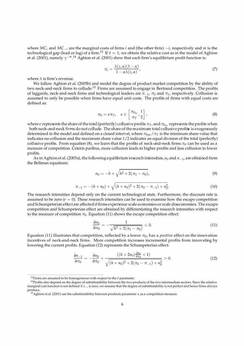
where MCi and MC−i are the marginal costs of firms i and (the other firm) −i, respectively and m is thetechnological gap (lead or lag) of a firm.13 If δ = 1, we obtain the relative cost as in the model of Aghionet al. (2001), namely γ−m.14 Aghion et al. (2001) show that each firm’s equilibrium profit function is:

π i =λ(z, α)(1 − α)

1 − αλ(z, α), (7)

where λ is firm’s revenue.We follow Aghion et al. (2005b) and model the degree of product market competition by the ability of

two neck-and-neck firms to collude.15 Firms are assumed to engage in Bertrand competition. The profitsof laggards, neck-and-neck firms and technological leaders are π −1, π 0 and π 1, respectively. Collusion isassumed to only be possible when firms have equal unit costs. The profits of firms with equal costs aredefined as:

π 0 = π T , ∈ π 0nc

π T ,

1

2 , (8)

where represents the share of the total (perfectly) collusive profits π T , andπ 0nc represents the profits when both neck-and-neck firms do not collude. The share of the maximum total collusive profits is exogenouslydetermined in the model and defined on a closed interval, where π 0nc/π T is the minimum share value thatindicates no collusion and the maximum share value 1/2 indicates an equal division of the total (perfectly)collusive profits. From equation (8), we learn that the profits of neck-and-neck firms π 0 can be used as ameasure of competition. Ceteris paribus, more collusion leads to higher profits and less collusion to lowerprofits.

As in Aghion et al. (2005a), the following equilibrium research intensities, n0 and n−1, are obtained fromthe Bellman equations:

n0 = −h +

h2 + 2(π 1 − π 0), (9)

n−1 = −(h + n0) +

(h + n0)2 + 2(π 0 − π −1) + n20. (10)

The research intensities depend only on the current technological state. Furthermore, the discount rate isassumed to be zero (r = 0). These research intensities can be used to examine how the escape competitionand Schumpeterian effect are affected if firms experience scale economies or scale diseconomies. The escapecompetition and Schumpeterian effect are obtained by differentiating the research intensities with respectto the measure of competition π 0. Equation (11) shows the escape competition effect:

∂n0

∂π 0= −

1 h2 + 2(π 1 − π 0)

< 0. (11)

Equation (11) illustrates that competition, reflected by a lower π 0, has a positive effect on the innovation

incentives of neck-and-neck firms. More competition increases incremental profits from innovating bylowering the current profits. Equation (12) represents the Schumpeterian effect:

∂n−1

∂π 0= −

∂n0

∂π 0+

((h + 2n0) ∂n0∂π 0

+ 1) (h + n0)2 + 2(π 0 − π −1) + n2

0

> 0. (12)

13Firms are assumed to be homogeneous with respect to the δ parameter.14Profits also depend on the degree of substitutability between the two products of the two intermediate sectors. Since the relative

marginal cost function is not defined if x−i is zero, we assume that the degree of substitutability is not perfect and hence firms alwaysproduce.

15Aghion et al. (2001) use the substitutability between products parameter α as a competition measure.

6



It shows that competition has a negative effect on the innovation incentives of laggard firms. Increasesin competition reduce the rents that these laggard firms can earn after they innovate and hence lead toa decrease in incremental profits from innovating. This decrease in their incremental profit lowers theirinnovation incentives.

Aghion et al. (2005b) show that the inverted-U relationship between competition and innovation de-pends on the escape competition effect and the Schumpeterian effect. Below the optimal level of compe-tition that enhances innovation, the escape competition effect dominates and beyond the optimal level of competition the Schumpeterian effect dominates. In the next section, we extend the model of Aghion et al.(2005b) to examine the effect of scale (dis)economies on the escape competition effect, the Schumpeterianeffect and the competition-innovation relationship.

2.3. The effect of a U-shaped average cost function on the competition-innovation relationship

Producing below or beyond the MES may lead to differences between the incremental profits frominnovating. Post innovation profits are affected by scale economies in two ways. First, after innovatingfirms receive a bonus (pay a penalty) since, operating below (above) MES, the innovation results in output

increases that are accompanied by less (more) than proportional increases in costs. Second, differences inscale economies can have an indirect effect, by changing the likelihood of collusion.16 Scale diseconomiesmake undercutting a less profitable strategy in the present due to increases in average costs. However, scalediseconomies may also foster competitive behavior by reducing the capacity to retaliate against competitivepricing. As a result, it is as yet unclear how a U-shaped average cost curve affects the ability to collude(Tirole, 1988).

However, we can investigate the direct effect of scale economies. To start with, the relationship betweenscale economies and the escape competition can be examined by differentiating equation (11) with respectto the incremental profits χ = π 1 − π 0:

∂2n0

∂π 0∂χ=

1

(h2 + 2 χ)3/2> 0. (13)

Equation (13) is used to examine the magnitude of the escape competition effect if incremental profits ( χ) of neck-and-neck firms change. Higher incremental profits result in a lower escape competition effect. Neck-and-neck firms with scale economies have higher post-innovation rents π 1 if their average costs decreasedue to firm growth. Large neck-and-neck firms with scale diseconomies have lower incremental profits χif they expect lower post-innovation rents π 1 and/or higher current profits π 0 due to collusive behavior.Consequently, these large firms experience a larger escape competition effect.17

Differentiating equation (12) with respect to the gap between the profit of a neck-and-neck and laggard bank (λ = π 0 − π −1), shows how the Schumpeterian effect is affected by this gap in profits:

∂2n−1

∂π 0∂λ= −

(h + 2n0) ∂n0∂π 0

+ 1

((h + n0)2 + 2λ + n20)3/2

> 0. (14)

The Schumpeterian effect is larger if the incremental profits (λ) from innovation of a laggard firm arehigher. Hence, laggard firms with scale economies are more likely to innovate, for a given level of com-petition. Scale economies affect the incremental profit λ = π 0 − π −1 since only laggards are subject tothe Schumpeterian effect. Post-innovation rents of laggards π 0 with scale diseconomies may be higher if these large firms are more likely to collude.18 The initial profits of laggards π −1 with scale diseconomiesmay be lower compared to firms on the MES, since scale diseconomies may suppress the profits that can be

16Although we discuss the possible links between scale economies and collusion in this paper, competition is not endogenouslydetermined in this paper and Aghion et al. (2005b).

17The escape competition effect is only smaller if firms with scale diseconomies are more likely to behave competitively (low π 0)and if this competitive behavior results in high incremental profits χ from innovation.

18However, the reverse is also possible, since the effect of scale diseconomies on collusion is ambiguous.

7



earned. Therefore, laggard firms with scale diseconomies that are more likely to collude after they innovateand experience suppressed current profits have higher incremental profits (λ) from innovation and a largerSchumpeterian effect.19

In sum, the magnitude of the escape competition and Schumpeterian effect depends on the current levelof the incremental profits, which in turn are affected by the scale (dis)economies of a bank. The influenceof scale economies on incremental profits is ambiguous and hence an empirical issue. The slope of theinverted-U relationship also depends on the magnitudes of the escape competition and Schumpeterianeffect. If banks indeed become 'too big to innovate' , larger escape competition and Schumpeterian effectsmay lead to a steeper inverted-U relationship between competition and innovation.

3. Data and Methodology

This section provides a short description of the data and presents innovation, scale economies andcompetition measures, as well as our set of control variables and our estimation strategy.

3.1. DataOur sample consists of a large number of individual banks over the period 1984-2004 in the United

States. On average, around 10,500 banks per year are included in the dataset. Information is gathered fromthe Call reports for Income and Condition provided by the Federal Reserve System. The Call Reports arequarterly income statement and balance sheet data that all federally insured banks are required to submitto the Federal Deposit Insurance Corporation (FDIC). The data cover all banks regulated by the FederalReserve System, the Federal Deposit and Insurance Corporation and the Comptroller of the Currency. Forthe purpose of this study, we include only independent banks, in order to avoid measurement problems,in particular when measuring competition.20 The Call Reports include complete balance sheet and incomestatement data. All data are expressed in 1984 U.S. dollars.

3.2. Measuring Innovation

In Aghion et al. (2001) and Aghion et al. (2005b), innovations result in changes in the unit labor re-quirement, as shown in Figure 1b in the previous section. In the empirical literature, relating shifts in acost function, i.e., technical change, to (process) innovation is not new (Subramanian and Nilakanta, 1996;Ruttan, 1997; Agrell et al., 2002; Bleaney and Wakelin, 2002). Our approach to measuring innovation fallsinto this tradition, and closely aligns with the theoretical concept of the technology gap as stipulated inAghion et al. (2001) and Aghion et al. (2005b).

The measurement of technical change has gone through a number of developments. For a long time,the econometric approach, led by Tinbergen (1942), consisted of including a time trend when estimatinga cost (or production) function. Likewise, using index number theory, Solow (1957) identified neutraltechnical change, with constant marginal rates of substitutions. Put differently, in line with Tinbergen(1942) and Solow (1957), a change in the cost curve in Figure 1b would be a parallel shift, leaving the(other) parameters in the cost function unaffected.

For the index numbers approach, Diewert (1976) and others that followed, added flexibility to the mea-surement of technical change, relaxing the assumption that the latter was constant. For the econometricapproach, Baltagi and Griffin (1988), by introducing a general index of technical change, relax the assump-tion that technical change is constant in time. In addition, building on advances by Gollop and Jorgenson(1980) and others, they allow for biased technical change, as marginal rates of substitution are allowed tovary over time. The result is depicted in Figure 1b, where a shift of the cost curve from t = 1 to t = 2 is not(necessarily) parallel, and can, for example, reflect a skill bias.21

19The Schumpeterian competition effect is only smaller if laggards with scale diseconomies are more likely to behave competitivelyand experience increases in their average costs (low π 0). These laggards have low incremental profits and are relatively less affected by an increase in competition.

20We selected independent banks using Call Report items RSSD9397, RSSD9001 and RSSD9365.21The relationship between biased technical change and innovation is explained in Acemoglu (2002).

8



The advances described so far, consist of adding flexibility to the aggregate cost function, which isthereby allowed to evolve over time. Since the cost function describes the process whereby firms are as-

sumed to minimize costs while producing output, the set of estimated parameters reflects the state of technology. What separates technical change from other means of minimizing costs (such as adjusting theinput mix or reducing waste), is the fact that whereas the latter measures use the currently implementedtechnology, technical change consists of the invention or adoption of a new technology. In an attempt toreconcile this view of technical change with the notion of estimating cost functions, early work by Hayamiand Ruttan (1970), Mundlak and Hellinghausen (1982) and Lau and Yotopoulos (1989) has focused on thenotion of a meta frontier. The latter encompasses the set of available technologies, across firms and/or acrosstime. In this view, technical change consists of the adoption of a new technology, and is measured againstthe benchmark meta frontier, which combines all available technologies.

Figure 2a is used to explain the concept of the meta frontier, with a simple example based on costminimization with two inputs (x1, x2) and a single output ( y) and for two firms I and II. In this example,there are two annual frontiers, for t = 1 and time t = 2. Each frontier represents the minimum cost curve

for a certain level of output, based on the available technology in period t. The cost efficiency of firm I,located at point E at time t = 1 is OD/OE. If firm I is at point C at t = 2, its efficiency is OB/OC. Figure2a also shows that a second firm, II, is located at point H and faces a cost efficiency of OG/OH at timet = 1. The dashed line that envelops the annual frontier in Figure 2a represents the minimum cost frontierover the whole period, or meta frontier. Innovation results in a lower gap between the annual minimumcost frontier and the meta frontier. Innovation is then reflected by changes in the technology gap, whichmeasures the difference between currently available technology and optimal, available technology over thewhole period with values between zero and one (i.e., the firm is on the meta frontier).22 At t = 1 the firmfaces a technology gap of OA/OD, which narrows to OA/OB at t = 2 as the firm improves its technologyset. While firm I faces a technology gap of OA/OD in period t = 1, the technology gap of firm II is smaller(OF/OG).

Figure 2: Technolog gaps in U.S. banking

(a) Meta frontier and technology gap

0

ABC

D

E

F

G

H

Frontier at t = 1

Frontier at t = 2

x 2

/ y

x1 / y

annual frontiers meta frontier

(b) Distribution of banks with a technology gap of 1

0

. 0 5

. 1

. 1 5

D e n s i t y

1985 1990 1995 2000 2005Year

Kernel density estimate

We follow recent work by Battese et al. (2004), O’Donnell et al. (2008) and Bos and Schmiedel (2007), andobtain technology gaps by, first, employing Stochastic Frontier Analysis (SFA) to estimate the minimumcost frontier available in each year, and second, enveloping the resulting annual cost frontiers to obtain a

22The notion of technology gaps has been first used by Krugman (1979) and proxied in the literature by total factor productivity(TFP) differentials (Griffith et al., 2004).

9



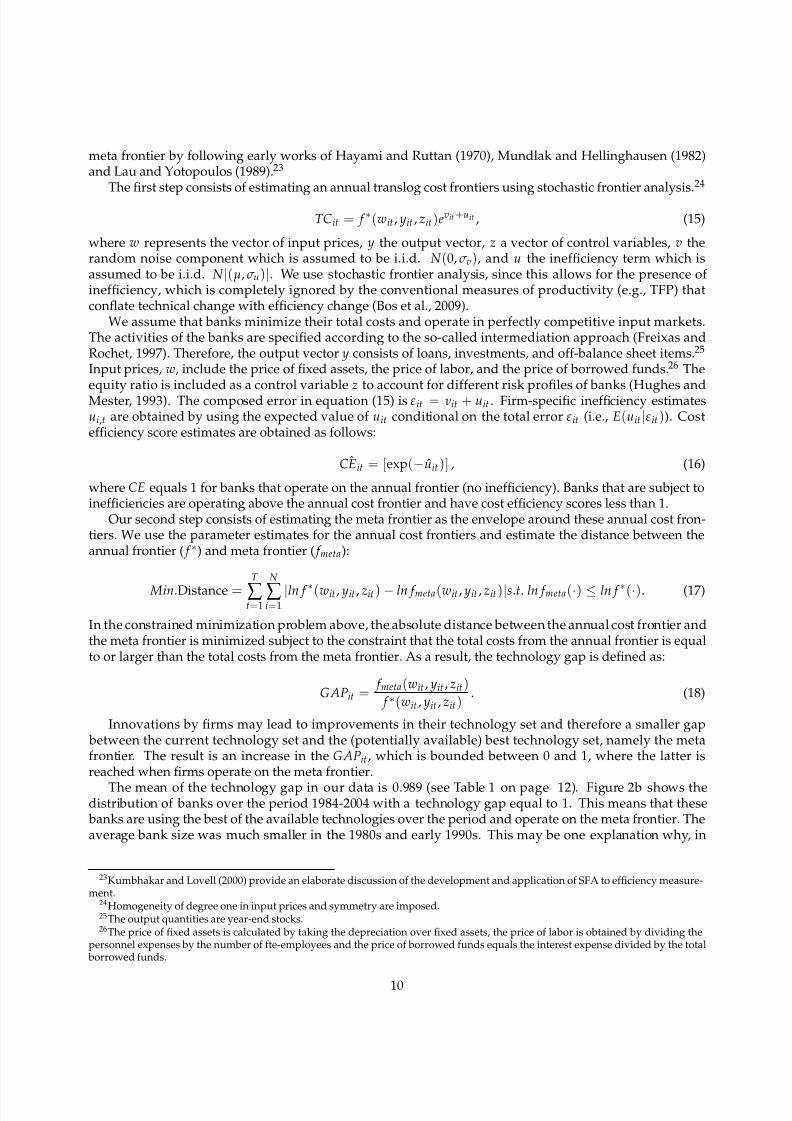
meta frontier by following early works of Hayami and Ruttan (1970), Mundlak and Hellinghausen (1982)and Lau and Yotopoulos (1989).23

The first step consists of estimating an annual translog cost frontiers using stochastic frontier analysis. 24

TCit = f ∗(wit , yit , zit )evit +uit , (15)

where w represents the vector of input prices, y the output vector, z a vector of control variables, v therandom noise component which is assumed to be i.i.d. N (0, σ v), and u the inefficiency term which isassumed to be i.i.d. N |(µ, σ u)|. We use stochastic frontier analysis, since this allows for the presence of inefficiency, which is completely ignored by the conventional measures of productivity (e.g., TFP) thatconflate technical change with efficiency change (Bos et al., 2009).

We assume that banks minimize their total costs and operate in perfectly competitive input markets.The activities of the banks are specified according to the so-called intermediation approach (Freixas andRochet, 1997). Therefore, the output vector y consists of loans, investments, and off-balance sheet items.25

Input prices, w, include the price of fixed assets, the price of labor, and the price of borrowed funds. 26 Theequity ratio is included as a control variable z to account for different risk profiles of banks (Hughes andMester, 1993). The composed error in equation (15) is εit = νit + uit . Firm-specific inefficiency estimatesui,t are obtained by using the expected value of uit conditional on the total error εit (i.e., E(uit |εit )). Costefficiency score estimates are obtained as follows:

ˆCEit = [exp(−uit )] , (16)

where CE equals 1 for banks that operate on the annual frontier (no inefficiency). Banks that are subject toinefficiencies are operating above the annual cost frontier and have cost efficiency scores less than 1.

Our second step consists of estimating the meta frontier as the envelope around these annual cost fron-tiers. We use the parameter estimates for the annual cost frontiers and estimate the distance between theannual frontier ( f ∗) and meta frontier ( f meta):

Min.Distance =

T

∑ t=1

N

∑ i=1

|ln f ∗(wit , yit , zit ) − ln f meta(wit , yit , zit )|s.t. ln f meta(·) ≤ ln f ∗(·). (17)

In the constrained minimization problem above, the absolute distance between the annual cost frontier andthe meta frontier is minimized subject to the constraint that the total costs from the annual frontier is equalto or larger than the total costs from the meta frontier. As a result, the technology gap is defined as:

GAPit =f meta(wit , yit , zit )

f ∗(wit , yit , zit ). (18)

Innovations by firms may lead to improvements in their technology set and therefore a smaller gap between the current technology set and the (potentially available) best technology set, namely the metafrontier. The result is an increase in the GAPit , which is bounded between 0 and 1, where the latter isreached when firms operate on the meta frontier.

The mean of the technology gap in our data is 0.989 (see Table 1 on page 12). Figure 2b shows thedistribution of banks over the period 1984-2004 with a technology gap equal to 1. This means that these banks are using the best of the available technologies over the period and operate on the meta frontier. Theaverage bank size was much smaller in the 1980s and early 1990s. This may be one explanation why, in

23Kumbhakar and Lovell (2000) provide an elaborate discussion of the development and application of SFA to efficiency measure-ment.

24Homogeneity of degree one in input prices and symmetry are imposed.25The output quantities are year-end stocks.26The price of fixed assets is calculated by taking the depreciation over fixed assets, the price of labor is obtained by dividing the

personnel expenses by the number of fte-employees and the price of borrowed funds equals the interest expense divided by the total borrowed funds.

10



this period, banks had an easier time reaching the meta frontier, given the amount of inputs and outputsinvolved in the production process. As banks increased in size, and presumably in complexity, bridgingthe technology gap can become more challenging. Another explanation for the same trend, however, may be a possible decline in competition during the sample period. We therefore now turn to our approach tomeasuring competition.

3.3. Measuring CompetitionWe measure competition in the banking sector by using one minus the price cost margin (viz., the Lerner

index, or markup) as in Aghion et al. (2005b):

Cit = 1 − (Πit + Fit

Rit), (19)

where Πit is the profit of a bank, Fit represents the fixed costs and Rit are the total sales of each bank. Theprice cost margin of a bank is obtained by dividing the net income after taxes and extraordinary itemsplus expenses of premises and fixed assets by total non-interest income plus total interest income. A firm-

specific measure of competition is preferred instead of using a measure based on a certain geographicalmarket as some banks compete mainly at the local level while other banks compete mainly at the nationalor international level. Hence, we assume that all changes in competition are reflected in the price costmargins of banks despite of the scope of the geographical market in which banks are competing. After theexclusion of outliers, the price cost margin and the competition measure range between -1 and 1, and 0 and2, respectively.27

3.4. Measuring Scale EconomiesWe employ two measures for scale economies. The first measure is a firm size measure based on total

assets.28 There should be a direct correlation between scale economies and firm size as firms that are belowthe MES are usually the (relatively) smaller firms in an industry. This measure, however, has two maindrawbacks. First, the firm size variable may capture other effects than scale economies in production.Second, while a certain firm size may be characterizing the MES in a given year, the same firm size may

indicate scale economies in other years (see Figure 1).An alternative measure is based on the elasticity of total costs with respect to the outputs. By using SFA,

we estimate cost functions and calculate the elasticity as follows:29

Scaleit =3

∑ k=1

∂ ln TCit

∂ ln ykit, (20)

where k indicates the three different outputs used in this paper, namely loans, investments and off-balancesheet items.

The SFA scale economies are calculated for a given output bundle keeping the output mix constant. 30 If the scale economies variable is equal to 1, the production is subject to constant returns to scale. If the valueis lower than 1, it indicates scale economies. Values larger than 1 indicate scale diseconomies. A drawbackof this measure is that it is a generated regressor that is constructed from a similar underlying procedure

that is used to obtain the technology gap.

27Scatterplots of the technology gap and the price cost margin were used to check for outliers. In total, 1324 observations (less than1% of the original sample) were excluded. A range of the price cost margin between -1 and 1 was considered to be reasonable. Someauthors choose to remove negative price cost margins, but this approach creates a bias in the results as only firms with positive pricecost margins are considered. The dataset contains 14,073 observations with negative price cost margins.

28The hypothesis that large firms are more than proportionally innovative compared to smaller firms is associated with the work of Schumpeter. There are many channels through which larger firms may have innovation advantages over smaller firms. For example,larger firms may have an advantage because they have more researchers which may lead to more productive interaction in this largeresearch group. It is also possible that larger firms are more able to diversify risky innovation projects.

29For example, see Hunter and Timme (1991), Bernstein (1996) and Altunbas et al. (2001) for applications of this scale economiesmeasure in the banking sector.

30As opposed to scale biased technical change, where technical change may result in a change of the cost-minimizing size of thefirm (Hunter and Timme, 1991).

11



3.5. Control variables

We include two control variables in our analysis. The equity ratio is included as a control variable toaccount for the relationship between the risk of a firm and innovation. Aghion et al. (2005b) argue that moredebt pressure has a positive effect on the innovation incentives of firms. This positive effect is interpretedas an attempt of firms to escape from their existing debt pressure through innovations. Furthermore, theaverage wage per fte-employee (salary expenses divided by the number of fte-employees) is also includedin our analysis as a proxy for human capital, as high quality workers may foster innovations (Funke andStrulik, 2000).31

Table 1: Descriptive statistics

Variable Mean Std. Dev. Minimum MaximumTechnology gap 0.989 0.029 1.07e-08 1 .000Price cost margin 0.179 0.090 -0.993 0.964

Total assets per millions of USD 458.740 7416.978 1.067 967,365Scale economies (from SFA) 1.099 0.071 0.726 1.737Risk (Equity/Total Assets) 0.096 0.034 7.36e-05 0.998Salary expenses per fte in thousands of USD 35.143 12.756 0.048 537.160

151,476 observations. The descriptive statistics are based on the sample of the preferred specifications in Table 2.

Table 1 provides the descriptive statistics of the variables employed in our analysis.32 We observe alarge spread in the price cost margin. Also, both scale economies (values smaller than unity) and scalediseconomies exist in our sample.

3.6. Empirical Specification

Our empirical specification is based on Aghion et al. (2005b), but extended to account for the impact of scale (dis)economies:

GAPit = β1Cit + β2C2it + β3Sit + β4Sit Cit + β5Sit C2

it + γZit + ai + εit , (21)

where GAP is the technology gap, C competition, S total assets or the SFA scale economies variable, γ 1xnparameter vector, and Z an nx1 vector of control variables. A squared term of the competition variable,C2, is included to account for the possible inverted-U relationship between competition and innovationaccording to Aghion et al. (2005). The interaction terms with the scale economies measure, SC and SC2,are included to allow the inverted-U relationship to be different for each firm due to differences in scaleeconomies.

The conditions in equation (13) and (14) show that the magnitude of the escape competition effect andSchumpeterian effect depends on the incremental profits that a firm can earn by innovating. Whether afirm experiences scale economies or scale diseconomies may affect this incremental profit and thereforethe magnitude of the escape competition effect, Schumpeterian effect and the steepness of the inverted-Urelationship. Taking first-differences of equation (21) to eliminate the unobserved heterogeneity ai gives:

∆GAPit = β1∆Cit + β2∆C2it + β3∆Sit + β4∆(Sit Cit ) + β5∆(Sit C2

it ) + γ∆Zit + ∆εit . (22)

We also estimate equation (22) replacing the continuous scale economies measure with a dummy variablethat indicates above average scale economies (1) or below average scale economies (0).

31We assume that the wages of high quality workers are higher.32The total number of observations is approximately 220,000 with on average 10,500 banks each year. Eventually, we have

151,476 observations in the preferred specification due to missing values of several variables, the exclusion of outliers, applyingfirst-differences, and using lags of the endogenous regressors as instruments.

12



While competition and scale economies affect innovation, innovation may also affect competition andscale economies. For example, firms may become more dominant in a market after surpassing other com-

petitors due to successful innovations.33 Innovations may also increase the MES. Therefore, lags of theseendogenous variables are used as instruments. The lag structure of the instruments depends on the orderof autocorrelation in the residuals.34 If the residual in equation (21) is not autocorrelated, lags of periodt-2 can be used as instruments for the endogenous regressors in equation (22). If there is first-order auto-correlation, lags from period t-3 and deeper can be used. Furthermore, we use the two-step generalizedmethod of moments estimator (GMM). The GMM has some efficiency gains compared to the traditionalinstrumental variable (IV) or two-stage least square (2SLS) estimators. For example, the two-step GMMestimator utilizes an optimal weighting matrix that minimizes the asymptotic variance of the estimator.Also, GMM is more efficient than the 2SLS estimator in the presence of heteroskedasticity.

4. Results

In this section, we present our results. First, we investigate the development of the scale economies,average bank size and the average price cost margin over time. Next, we explore whether U.S. banks have become too big to innovate.

4.1. How have scale economies and competition developed in the consolidating U.S. banking market?

The model of Aghion et al. (2001) and Aghion et al. (2005b) analyzes how banks’ innovative behaviorchanges as their competitive position changes. The resulting market dynamic is therefore grounded infirm-level differences. If there is no room to explore scale economies, banks are less able to reap the bonusthat awaits them when they innovate. Likewise, if there are no banks operating beyond their MES, there isno such thing as being 'too big to innovate'.

Figure 3: Scale economies, total assets and the price cost margin

(a) Distribution of scale economies in 1984, 1995 and 2004

0

5

1 0

1 5

2 0

D e n s i t y

.6 .8 1 1.2 1.4 1.6

scale economies

1984 1995 2004

Kernel density estimates, based on estimates of annual translog cost frontiers.

(b) Average total assets and the price cost margin

. 1

. 1 5

. 2

. 2 5

A v e r a g e p r i c e c o s t m a r g i n

. 2

. 4

. 6

. 8

1

A v e r a g e t o t a l a s s e t s ( U S D

1 b n )

1985 1990 1995 2000 2005

Year

Price cost margin Total assets (USD1 mln)

Annual, unweighted averages

Figure 3a shows how the distribution of scale economies has evolved over our sample period. Thefigure shows two concurrent developments. First, the number of banks with scale diseconomies has grownover time. Second, as the market consolidated, the distribution of scale economies narrowed mid sample

33However, Geroski and Pomroy (1990) argue that more innovations may lead to more competition.34The Arellano-Bond autocorrelation test is based on the examination of residuals in first differences. Testing for first-order serial

correlation in levels is based on testing for second-order serial correlation in first differences.

13



(i.e., in 1995), but widened again towards the end of the sample period. Summing up, Figure 3a reflects aconsolidating market, with plenty of differences in the potential penalty (or bonus) for innovators.

The story of a consolidating market is repeated in Figure 3b, which shows the development of average bank size (total assets in $bn) and the average price cost margin over the sample period. Interestingly, thepeak in the price cost margin more or less coincides with the mid sample period, when the market wasat its most homogenous in terms of scale economies. As Figure 3b shows, competition has decreased, onaverage, over the sample period. This finding is consistent with the results of Stiroh and Strahan (2003),who argue that the banking deregulation ignited a reallocation of banking assets from low profit to highprofit banks. Meanwhile, the average bank size increased from total assets around 165 million dollars toaround 936 million dollars in 2004.

The developments in scale economies and competition, together with the development of the technol-ogy gap described in Figure 2b, tell the story of a market with a lot of dynamics, and plenty of potential for banks to become 'too big to innovate'. The latter issue is investigated further in the next subsection.

4.2. Have large US banks become too big to innovate?

In this section, we investigate the influence of scale economies on the competition-innovation relation-ship. Before we examine whether large US banks have indeed become 'too big to innovate', we need toestablish the overall nature of the competition-innovation relationship.

We therefore start with the first set of estimation results in Table 2, where we estimate the basic modelspecification, including control variables and total assets, but without allowing for a possible effect of thelatter on the competition-innovation relationship. The results are shown in columns (i) and (ii), where wereport both OLS (in column (i)) and two-step GMM (in column (ii)) estimates.35 As is clear from the sig-nificant positive (negative) relationship for the competition measure (squared competition measure), thereis indeed an inverted-U competition-innovation relationship: as competition increases, innovation initiallyrises, until it reaches a peak, after which the Schumpeterian competition effect dominates. 36 Interestingly,the optimal price cost margin that enhances innovation is 5.8%. Looking back at Figure 3b, we observe thaton average this price cost margin is first reached around 1992, and again around the year 2000. Of course,comparing with Figure 3a, we know that a major difference between these two (sub-)periods lies with thedevelopment of scale economies.

These results are in line with Bos et al. (2009), who also report an inverted-U relationship for U.S. bank-ing. In line with Aghion et al. (2005b), we find that banks with a higher equity ratio feel less debt pressureand are as a result less innovative. In our (preferred) GMM specification, a higher average wage has noeffect, reflecting the fact that human capital has no considerable effect on banks’ (process) innovativeness.And although firm size (S) is statistically significant at the 5% level in column (i), there is no evidence of asignificant relationship between firm size and the technology gap once we treat the competition variablesas endogenous regressors (column (ii)).37

Next, we proceed by investigating whether large U.S. banks have become to 'too big to innovate'. Tothis purpose, we allow interaction between scale economies and competition, so we can measure the effectof scale economies on the competition-innovation relationship. To accurately study this effect, we includescale economies in three different ways, presented in columns (iii), (iv) and (v) of Table 2. Each approach

has its own advantages. In the first approach, presented in column (iii), scale is accounted for by banks’total assets. The advantages of this scale measure are that it is continuous, and (presumably) preciselymeasurable.38 Therefore, we shall use this estimation in comparison with the earlier described results, in

35For the GMM estimation, we use instruments from periods t − 3 and t − 4, since there is evidence of first-order autocorrelation inthe residuals in levels. The instruments are relevant and valid according to first-stage F-tests and the Hansen test, respectively. Theinstrument relevance test is based on the joint significance of the instruments, with a critical value for the F-statistic of 10 applied asan often used rule of thumb. The F-statistics for the regressions with the competition variable and its squared term as a dependentvariable are 413.84 and 251.56, respectively.

36Both competition variables are individually and jointly significant at the 1% level.37There is also no significant effect of firm size on the technology gap if we treat the firm size variable as endogenous with lags

from period t-3 and t-4 as instruments. In the remaining part of the paper we do not examine the marginal effect of firm size on thetechnology gap and focus only on the (conditional) marginal effect of competition on the technology gap.

38A possible disadvantage is that other things besides scale economies may affect the competition-innovation relationship.

14



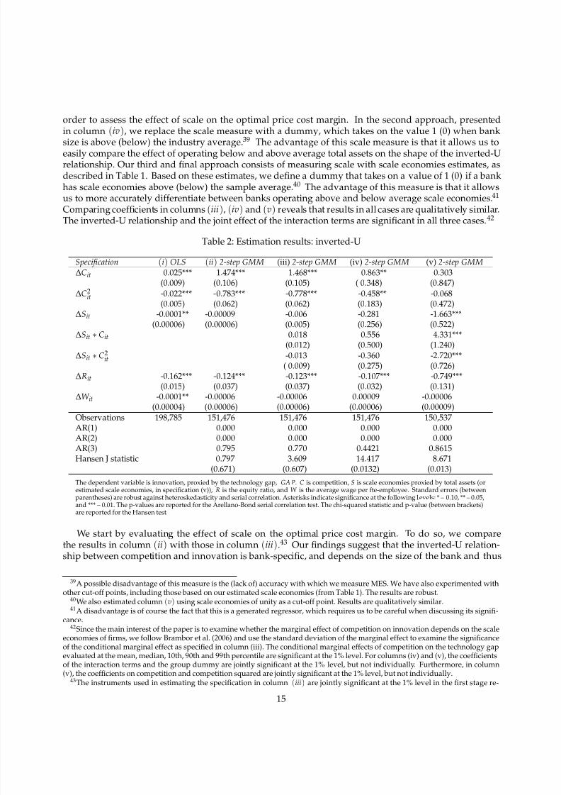
order to assess the effect of scale on the optimal price cost margin. In the second approach, presentedin column (iv), we replace the scale measure with a dummy, which takes on the value 1 (0) when bank

size is above (below) the industry average.39 The advantage of this scale measure is that it allows us toeasily compare the effect of operating below and above average total assets on the shape of the inverted-Urelationship. Our third and final approach consists of measuring scale with scale economies estimates, asdescribed in Table 1. Based on these estimates, we define a dummy that takes on a value of 1 (0) if a bankhas scale economies above (below) the sample average.40 The advantage of this measure is that it allowsus to more accurately differentiate between banks operating above and below average scale economies.41

Comparing coefficients in columns (iii), (iv) and (v) reveals that results in all cases are qualitatively similar.The inverted-U relationship and the joint effect of the interaction terms are significant in all three cases. 42

Table 2: Estimation results: inverted-U

Specification (i) OLS (ii) 2-step GMM (iii) 2-step GMM (iv) 2-step GMM (v) 2-step GMM

∆Cit

0.025*** 1.474*** 1.468*** 0.863** 0.303(0.009) (0.106) (0.105) ( 0.348) (0.847)

∆C2it -0.022*** -0.783*** -0.778*** -0.458** -0.068

(0.005) (0.062) (0.062) (0.183) (0.472)∆Sit -0.0001** -0.00009 -0.006 -0.281 -1.663***

(0.00006) (0.00006) (0.005) (0.256) (0.522)∆Sit ∗ Cit 0.018 0.556 4.331***

(0.012) (0.500) (1.240)

∆Sit ∗ C2it -0.013 -0.360 -2.720***

( 0.009) (0.275) (0.726)∆Rit -0.162*** -0.124*** -0.123*** -0.107*** -0.749***

(0.015) (0.037) (0.037) (0.032) (0.131)∆W it -0.0001** -0.00006 -0.00006 0.00009 -0.00006

(0.00004) (0.00006) (0.00006) (0.00006) (0.00009)

Observations 198,785 151,476 151,476 151,476 150,537AR(1) 0.000 0.000 0.000 0.000AR(2) 0.000 0.000 0.000 0.000AR(3) 0.795 0.770 0.4421 0.8615Hansen J statistic 0.797 3.609 14.417 8.671

(0.671) (0.607) (0.0132) (0.013)

The dependent variable is innovation, proxied by the technology gap, GA P. C is competition, S is scale economies proxied by total assets (orestimated scale economies, in specification (v)), R is the equity ratio, and W is the average wage per fte-employee. Standard errors (betweenparentheses) are robust against heteroskedasticity and serial correlation. Asterisks indicate significance at the following l evels: * – 0.10, ** – 0.05,and *** – 0.01. The p-values are reported for the Arellano-Bond serial correlation test. The chi-squared statistic and p-value (between brackets)are reported for the Hansen test.

We start by evaluating the effect of scale on the optimal price cost margin. To do so, we comparethe results in column (ii) with those in column (iii).43 Our findings suggest that the inverted-U relation-

ship between competition and innovation is bank-specific, and depends on the size of the bank and thus

39A possible disadvantage of this measure is the (lack of) accuracy with which we measure MES. We have also experimented withother cut-off points, including those based on our estimated scale economies (from Table 1). The results are robust.

40We also estimated column (v) using scale economies of unity as a cut-off point. Results are qualitatively similar.41A disadvantage is of course the fact that this is a generated regressor, which requires us to be careful when discussing its signifi-

cance.42Since the main interest of the paper is to examine whether the marginal effect of competition on innovation depends on the scale

economies of firms, we follow Brambor et al. (2006) and use the standard deviation of the marginal effect to examine the significanceof the conditional marginal effect as specified in column (iii). The conditional marginal effects of competition on the technology gapevaluated at the mean, median, 10th, 90th and 99th percentile are significant at the 1% level. For columns (iv) and (v), the coefficientsof the interaction terms and the group dummy are jointly significant at the 1% level, but not individually. Furthermore, in column(v), the coefficients on competition and competition squared are jointly significant at the 1% level, but not individually.

43The instruments used in estimating the specification in column (iii) are jointly significant at the 1% level in the first stage re-

15



whether the bank experiences scale economies or scale diseconomies. The average optimal price cost mar-gin for banks with total assets more than $654,000,000 (95th percentile) is around 7.3%, compared to the

5.8% found earlier. However, on average the actual price cost margin for these banks 18.8%.44 Interestingly,these high rents cannot be explained by cost advantages, as these banks operate beyond the MES. The co-efficients on the interaction terms indicate that the innovation behavior of larger banks is more responsiveto changes in competition. Hence, the innovation incentives of large banks are diminishing if these bankscontinue to earn higher rents in the future.

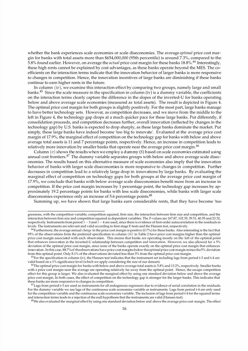
In column (iv), we examine this interaction effect by comparing two groups, namely large and small banks.45 Since the scale measure in the specification in column (iv) is a dummy variable, the coefficientson the interaction terms clearly capture the difference in the slopes of the inverted-U for banks operating below and above average scale economies (measured as total assets). The result is depicted in Figure 4.The optimal price cost margin for both groups is slightly positively. For the most part, large banks manageto have better technology sets. However, as competition decreases, and we move from the middle to theleft in Figure 4, the technology gap drops at a much quicker pace for these large banks. Put differently, if

consolidation proceeds, and competition decreases further, overall innovation (reflected by changes in thetechnology gap) by U.S. banks is expected to drop sharply, as these large banks dominate the market. Putsimply, these large banks have indeed become 'too big to innovate'. Evaluated at the average price costmargin of 17.9%, the marginal effect of competition on the technology gap for banks with below and aboveaverage total assets is 11 and 7 percentage points, respectively. Hence, an increase in competition leads torelatively more innovation by smaller banks that operate near the average price cost margin. 46

Column (v) shows the results when we employ a dummy (S) based on scale economies estimated usingannual cost frontiers.47 The dummy variable separates groups with below and above average scale disec-onomies. The results based on this alternative measure of scale economies also imply that the innovation behavior of banks with larger scale diseconomies is more responsive to changes in competition. Furtherdecreases in competition lead to a relatively large drop in innovations by large banks. By evaluating themarginal effect of competition on technology gaps for both groups at the average price cost margin of 17.9%, we conclude that banks with below average scale diseconomies benefit more from an increase incompetition. If the price cost margin increases by 1 percentage point, the technology gap increases by ap-proximately 19.2 percentage points for banks with less scale diseconomies, while banks with larger scalediseconomies experience only an increase of 5.6 percentage points.48

Summing up, we have shown that large banks earn considerable rents, that they have become 'too

gressions, with the competition variable, competition squared, firm size, the interaction between firm size and competition, and theinteraction between firm size and competition squared as dependent variables. The F-values are 167.87, 102.35, 39.51, 40.55 and 23.32,respectively. Instruments from period t − 3 and t − 4 are used, since there is evidence of first-order autocorrelation in the residuals inlevels. The instruments are relevant and valid according to first-stage F-tests and the Hansen test, respectively.

44Furthermore, the average annual change in the price cost margin is positive (0.7%) for these banks. Also interesting is the fact that95% of the observations from the preferred specification in column (iii) in Table 2 have price cost margins higher than the optimalprice cost margin associated with each observation. This means that banks are operating mostly on the left of the optimal pointthat enhances innovation in the inverted-U relationship between competition and innovation. However, we also allowed for a 5%

deviation of the optimal price cost margin, since none of the banks operate exactly on the optimal price cost margin that enhancesinnovation. In this case, 88.7%of theobservations have price cost margins below theoptimal price cost margin minus the5% deviationfrom this optimal point. Only 8.1% of the observations deviated less than 5% from the optimal price cost margin.

45For the specification in column (iv), the Hansen test indicates that the instrument set including lags from period t-3 and t-4 arevalid based on a 1% significance level (which we apply considering the size of our dataset).

46The optimal price cost margin for banks with below and above average total assets is 5.8% and 13.2%, respectively. Smaller bankswith a price cost margin near the average are operating relatively far away from the optimal point. Hence, the escape competitioneffect for this group is larger. We also evaluated the marginal effect by using one standard deviation below and above the averageprice cost margin. In both cases, the effect of competition on the technology gap is stronger for the larger banks. This indicates thatthese banks are more responsive to changes in competition.

47Lags from period t-3 are used as instruments for all endogenous regressors due to evidence of serial correlation in the residuals.For the dummy variable we use lags of the continuous scale economies variable as instruments. Lags from period t-4 are only usedfor the competition variable and the continuous scale economies variable. The inclusion of lags from period t-4 for the squared termsand interaction terms leads to a rejection of the null hypothesis that the instruments are valid (Hansen test).

48We also evaluated the marginal effect by using one standard deviation below and above the average price cost margin. The effect

16



Figure 4: The competition-innovation relationship

− . 4

− . 2

0

. 2

. 4

. 6

P r e d i c t e d

t e c h n o l o g y g a p

0 .5 1 1.5 21−price cost margin

Below average to ta l assets Above average to tal assets

big to innovate', and that the effect on innovation is sizeable. Added to the ongoing consolidation in U.S. banking, these results suggest that policies aimed at increasing competition may have an important positiveexternality: in addition to the usual downward pressure on prices, increased competition may, ironically,result in further cost reductions, as large banks in particular try to escape competition by innovating.

5. Conclusion

This paper has examined the effect of scale (dis)economies on the competition-innovation relationshipin U.S. banking. Theoretical endogenous growth models have ignored this effect, as they rely on thepremise that unit costs are independent from output levels. Such models are less appropriate for inves-

tigating the effect of competition on innovation in sectors where average costs are not constant.We have extended the theoretical model of Aghion and Griffith (2005) to allow for a U-shaped average

cost curve where firms may operate below, on or beyond the MES. The latter constitutes a novelty of thispaper as it allows us to derive conditions under which the magnitude of the Schumpeterian effect andescape competition effect differs between firms. Firms that operate below the MES have a higher bonuswhen they innovate since they experience more potential for growth. The (process) innovation lowerstheir average costs, and thereby increases the expected rents from innovating. Firms that operate beyondthe MES have less growth potential since firm growth may increase their average costs.

In addition we have introduced a novel way to measure process innovation in banking. The measure of innovation that we utilize focuses on banks’ ability to minimize costs through innovations. Innovations im-prove the technology sets of banks and narrow the technological distance between the technology appliedin a bank and the best (potential) available technology. Relying on recent contributions to the estimation of

meta cost frontiers, we measure these technology gaps.Subsequently, we have tested the theoretical implications of our model on a rich data set of U.S. banks.Our main aim was to find whether large U.S. banks have become 'too big to innovate'. We find that most banks in the U.S. start to operate beyond the Minimum Efficient Scale and experience scale diseconomies asthe sector consolidates and average bank sizes increase. The upward trend in the average price cost marginsduring the same period implies that the degree of competition in the banking sector has declined. Ourresults provide support of an inverted-U relationship between competition and innovation in U.S. banking.This finding is robust over several different model specifications and consistent with the theoretical andempirical work of Aghion et al. (2005b) and Bos et al. (2009).

of competition on the technology gap is stronger for banks with larger scale diseconomies in both cases. This indicates that these banks are more responsive to changes in competition.

17



Further analysis has revealed the effect of scale (dis)economies on the nature of the competition-innovationrelationship in U.S. banking. Large banks are shown to earn considerable rents. Important, the inverted-Urelationship between competition and innovation becomes steeper as bank size increases. Our findingshave important implications for competition policy. As banks, on average, are becoming larger over time,the increased responsiveness in terms of innovation should be taken into account when implementing com-petition policies. Any further decreases in competition will prove to be highly detrimental to innovation,due to the more than proportional reduction in innovation by large banks that have become 'too big toinnovate'. In contrast, the added bonus of any policy that effectively stimulates competition is a boost ininnovation, due to its effect on large banks.

References

Acemoglu, D., 2002. Directed technical change. Review of Economic Studies 69 (4), 781–809.Acs, Z. J., Audretsch, D. B., 1987. Innovation in large and small firms. Economics Letters 23 (1), 109–112.Aghion, P., Bloom, B., Blundell, R., Griffith, R., Howitt, P., 2005a. Competition and innovation: An inverted U relationship. NBER

Working Paper 9269.Aghion, P., Bloom, N., Blundell, R., Griffith, R., Howitt, P., 2005b. Competition and innovation: An inverted-U relationship. Quarterly

Journal of Economics 120 (2), 701–728.Aghion, P., Griffith, R., 2005. Competition and Growth: Reconciling Theory and Evidence. MIT Press, Cambridge, Mass.Aghion, P., Harris, C., Howitt, P., Vickers, J., 2001. Competition, imitation and growth with step-by-step innovation. Review of Eco-

nomic Studies 68 (3), 467–492.Aghion, P., Harris, C., Vickers, J., 1997. Competition and growth with step-by-step innovation: An example. European Economic

Review 41 (3-5), 771–782.Agrell, P. J., Bogetoft, P., Tind, J., Jul. 2002. Incentive plans for productive efficiency, innovation and learning. International Journal of

Production Economics 78 (1), 1–11.Altunbas, Y., Gardener, E. P. M., Molyneux, P., Moore, B., 2001. Efficiency in European banking. European Economic Review 45 (10),

1931–1955.Baltagi, B. H., Griffin, J. M., 1988. A general index of technical change. Journal of Political Economy 96 (1), 20–41.Battese, G. E., Rao, D. S. P., O’Donnell, C. J., 2004. A metafrontier production function for estimation of technical efficiencies and

technology gaps for firms operating under different technologies. Journal of Productivity Analysis 21 (1), 91–103.Berger, A. N., 2003. The economic effects of technological progress: Evidence from the banking industry. Journal of Money, Credit and

Banking 35 (2), 141–76.Berger, A. N., Demirguc-Kunt, A., Levine, R., Haubrich, J., 2004. Bank concentration and competition: An evolution in the making. Journal of Money, Credit and Banking 36 (3), 433–451.

Berger, A. N., Demsetz, R. S., Strahan, P. E., Feb. 1999. The consolidation of the financial services industry: Causes, consequences, andimplications for the future. Journal of Banking and Finance 23 (2-4), 135–194.

Berger, A. N., DeYoung, R., 2006. Technological progress and the geographic expansion of the banking industry. Journal of Money,Credit and Banking 38 (6), 1483–1513.

Berger, A. N., Hannan, T. H., 1989. The price-concetration relationship in banking. Review of Economics and Statistics 71 (2), 291–299.Berger, A. N., Kashyap, A. K., Scalise, J. M., 1995. The transformation of the U.S. banking industry: What a long, strange trips it’s

been. Brookings Papers on Economic Activity 26 (1995-2), 55–218.Bernstein, D., 1996. Asset quality and scale economies in banking. Journal of Economics and Business 48 (2), 157–166.Bleaney, M., Wakelin, K., 2002. Efficiency, innovation and exports. Oxford Bulletin of Economics and Statistics 64 (1), 3–15.Bos, J. W. B., Kolari, J. W., van Lamoen, R., 2009. Competition and innovation: Evidence from financial services. TKI Working Paper

09-16, Tjalling Koopmans Institute, Utrecht School of Economics.Bos, J. W. B., Schmiedel, H., 2007. Is there a single frontier in a single European banking market? Journal of Banking and Finance

31 (7), 2081–2102.

Brambor, T., Clark, W., Golder, M., 2006. Understanding interaction models: Improving empirical analyses. Political Analysis 14 (1),63–82.

Carletti, E., Hartmann, P., Spagnolo, G., 2007. Bank mergers, competition, and liquidity. Journal of Money, Credit and Banking 39 (5),1067–1105.

Celent, 2009. IT spending in financial services: A global perspective. News article 1009, Money Science,http://www.moneyscience.com/Technology _News/article1009.

Cetorelli, N., Strahan, P. E., 2006. Finance as a barrier to entry: Bank competition and industry structure in local u.s. markets. The Journal of Finance 61 (1), 437–461.

Cole, R. A., Goldberg, L. G., White, L. J., 2004. Cookie cutter vs. character: The micro structure of small business lending by large andsmall banks. Journal of Financial and Quantitative Analysis 39 (2), 227–251.

DeYoung, R., Hunter, W. C., 2001. Deregulation, the internet, and the competitive viability of large banks and community banks.Working Paper Series WP-01-11, Federal Reserve Bank of Chicago.

Diewert, W. E., May 1976. Exact and superlative index numbers. Journal of Econometrics 4 (2), 115–145.Frame, W. S., White, L. J., 2004. Empirical studies of financial innovation: Lots of talk, little action? Journal of Economic Literature

42 (1), 116–144.

18



Freixas, X., Rochet, J., 1997. Microeconomics of Banking. MIT Press, Cambridge.Funke, M., Strulik, H., 2000. On endogenous growth with physical capital, human capital and product variety. European Economic

Review 44 (3), 491–515.

Geroski, P. A., 1990. Innovation, technological opportunity, and market structure. Oxford Economic Papers 42 (3), 586–602.Geroski, P. A., Pomroy, R., 1990. Innovation and the evolutionof market structure. The Journal of Industrial Economics 38 (3), 299–314.Gollop, F. M., Jorgenson, D. W., 1980. U.S. productivity growth by industry, 1947-73. In: Kendrick, J. W., Vaccara, B. N. (Eds.), New

Developments in Productivity Measurement and Analysis. University Chicago Press (for NBER), Chicago, pp. –.Griffith, R., Redding, S., Reenen, J. V., 2004. Mapping the two faces of R&D: Productivity growth in a panel of OECD industries. The

Review of Economics and Statistics 86 (4), 883–895.Griliches, Z., 1990. Patent statistics as economic indicators: A survey. Journal of Economic Literature 28 (4), 1661–1707.Hannan, T. H., McDowell, J. M., 1984. The determinants of technology adoption: The case of the banking firm. Rand Journal of

Economics 15 (3), 328–335.Hashmi, A., 2007. Competition and innovation: The inverted-U relationship revisited. Working paper, University of Toronto.Hayami, Y., Ruttan, V. W., 1970. Agricultural productivity differences among countries. American Economic Review 60 (5), 895–911.Hughes, J. P., Mester, L. J., 1993. A quality and risk-adjusted cost function for banks: Evidence on the "too-big-to-fail" doctrine. Journal

of Productivity Analysis 4 (3), 293–315.Hunter, W. C., Timme, S. G., 1991. Technological change in large U.S. commercial banks. Journal of Business 64 (3), 339–362. Jones, K. D., Critchfield, T., 2005. Consolidation in the U.S. banking industry: Is the "long, strange trip" about to end? FDIC Banking

Review 17 (4), 31–61.

Kamien, M. I., Schwartz, N. L., 1982. Market Structure and Innovation. Cambridge University Press, New York, NY, USA.King, R. G., Levine, R., 1993. Finance and growth: Schumpeter might be right. Quarterly Journal of Economics 108 (3), 717–737.Krugman, P., 1979. A model of innovation, technology transfer, and the world distribution of income. Journal of Political Economy

87 (2), 253–266.Kumbhakar, S. C., Lovell, C. A. K., 2000. Stochastic Frontier Analysis. Cambridge University Press.Lau, L. J., Yotopoulos, P. A., 1989. The meta-production function approach to technological change in world agriculture. Journal of

Development Economics 31 (2), 241–269.Levin, R. C., W. M. C., Mowrey, D. C., 1985. R&D appropriability, opportunity, and market structure: New evidence on some Schum-

peterian hypotheses. American Economic Review 75 (2), 20–24.Levine, R., 2004. Finance and growth: Theory and evidence. Working Paper Series No. 10766, National Bureau of Economic Research.Levine, R., Loayza, N., Beck, T., 2000. Financial intermediation and growth: Causality and causes. Journal of Monetary Economics 46,

31–77.Melvin, M., Taylor, M. P., 2009. The crisis in the foreign exchange market. Journal of International Money and Finance 28 (8), 1317–

1330.Mishkin, F. S., Strahan, P. E., 1999. What will technology do to financial structure? In: NBER Working Papers. No. 6892 in NBER

Papers in Monetary Economics. National Bureau of Economic Research, Inc, p. 41.Mundlak, Y., Hellinghausen, R., 1982. The intercountry agricultural production function: Another view. American Journal of Agricul-

tural Economics 64 (4), 664–672.O’Donnell, C., Rao, D., Battese, G., 2008. Metafrontier frameworks for the study of firm-level efficiencies and technology ratios.

Empirical Economics 34 (2), 231–255.Pagano, M., 1993. Financial markets and growth: An overview. European Economic Review 37 (2-3), 613–622.Rhoades, S. A., 2000. Bank mergers and banking structure in the United States, 1980-98. Board of Governors of the Federal Reserve

System Staff Studies 174.Ruttan, V. W., 1997. Induced innovation, evolutionary theory and path dependence: Sources of technical change. The Economic

Journal 107 (444), 1520–1529.Scherer, F. M., 1967. Marketstructure andthe employment of scientists andengineers. TheAmericanEconomicReview 57 (3), 524–531.Schumpeter, J. A., 1942. Capitalism, Socialism and Democracy. Harper and Row, New York.Solow, R. M., 1957. Technical change and the aggregate production function. The Review of Economics and Statistics 39 (3), 312–320.Stiroh, K. J., Strahan, P. E., 2003. Competitive dynamics of deregulation: Evidence from u.s. banking. Journal of Money, Credit and

Banking 35 (5), 801–828.Subramanian, A., Nilakanta, S., Dec. 1996. Organizational innovativeness: Exploring the relationship between organizational deter-

minants of innovation, types of innovations, and measures of organizational performance. Omega 24 (6), 631–647.Symeonidis, G., 1996. Innovation, firm size and market structure: Schumpeterian hypotheses and some new themes. OECD Eco-nomics Department Working Paper 161.

Tinbergen, J., 1942. Zur theorie der langfristigen wirtschaftsentwicklung. Weltwirtschafliches Archiv 55 (1), 511–549.Tirole, J., 1988. The Theory of Industrial Organization. The MIT Press, Cambridge, MA.Vives, X., 2001. Competition in the changing world of banking. Oxford Review of Economic Policy 17 (4), 535–547.

19

Documents

Too Big to Innovate