Tom Loredo Dept. of Astronomy, Cornell University http ...astrostatistics.psu.edu/su09/lecturenotes/bayesLoredo.pdf · Bayesian inference quantiﬁes uncertainty by reporting probabilities

Introduction to Bayesian Inference

Tom LoredoDept. of Astronomy, Cornell University

http://www.astro.cornell.edu/staff/loredo/bayes/

CASt Summer School — June 11, 2008

1 / 111

Outline1 The Big Picture

2 Foundations—Logic & Probability Theory

3 Inference With Parametric ModelsParameter EstimationModel Uncertainty

4 Simple ExamplesBinary OutcomesNormal DistributionPoisson Distribution

5 Measurement Error Applications

6 Bayesian Computation

7 Probability & Frequency

8 Endnotes: Hotspots, tools, reflections

2 / 111









3 / 111

Scientific Method

Science is more than a body of knowledge; it is a way of thinking.The method of science, as stodgy and grumpy as it may seem,

is far more important than the findings of science.—Carl Sagan

Scientists argue!

Argument ≡ Collection of statements comprising an act ofreasoning from premises to a conclusion

A key goal of science: Explain or predict quantitativemeasurements (data!)

Data analysis constructs and appraises arguments that reason fromdata to interesting scientific conclusions (explanations, predictions)

4 / 111

The Role of Data

Data do not speak for themselves!

We don’t just tabulate data, we analyze data.

We gather data so they may speak for or against existinghypotheses, and guide the formation of new hypotheses.

A key role of data in science is to be among the premises inscientific arguments.

5 / 111

Data AnalysisBuilding & Appraising Arguments Using Data

Statistical inference is but one of several interacting modes ofanalyzing data.

6 / 111

Bayesian Statistical Inference

• A different approach to all statistical inference problems (i.e.,not just another method in the list: BLUE, maximumlikelihood, χ2 testing, ANOVA, survival analysis . . . )

• Foundation: Use probability theory to quantify the strength ofarguments (i.e., a more abstract view than restricting PT todescribe variability in repeated “random” experiments)

• Focuses on deriving consequences of modeling assumptionsrather than devising and calibrating procedures

7 / 111

Frequentist vs. Bayesian Statements

“I find conclusion C based on data Dobs . . . ”

Frequentist assessment

“It was found with a procedure that’s right 95% of the timeover the set Dhyp that includes Dobs.”Probabilities are properties of procedures, not of particularresults.

Bayesian assessment

“The strength of the chain of reasoning from Dobs to C is0.95, on a scale where 1= certainty.”Probabilities are properties of specific results.Performance must be separately evaluated (and is typicallygood by frequentist criteria).

8 / 111









9 / 111

Logic—Some Essentials“Logic can be defined as the analysis and appraisal of arguments”

—Gensler, Intro to Logic

Build arguments with propositions and logicaloperators/connectives

• Propositions: Statements that may be true or false

P : Universe can be modeled with ΛCDM

A : Ωtot ∈ [0.9, 1.1]

B : ΩΛ is not 0

B : “not B,” i.e., ΩΛ = 0

• Connectives:

A ∧ B : A andB are both true

A ∨ B : A orB is true, or both are

10 / 111

Arguments

Argument: Assertion that an hypothesized conclusion, H, followsfrom premises, P = A,B,C , . . . (take “,” = “and”)

Notation:

H|P : Premises P imply H

H may be deduced from PH follows from PH is true given that P is true

Arguments are (compound) propositions.

Central role of arguments → special terminology for true/false:

• A true argument is valid

• A false argument is invalid or fallacious

11 / 111

Valid vs. Sound Arguments

Content vs. form

• An argument is factually correct iff all of its premises are true(it has “good content”).

• An argument is valid iff its conclusion follows from itspremises (it has “good form”).

• An argument is sound iff it is both factually correct and valid(it has good form and content).

We want to make sound arguments. Formal logic and probabilitytheory address validity, but there is no formal approach foraddressing factual correctness → there is always a subjectiveelement to an argument.

12 / 111

Factual Correctness

Although logic can teach us something about validity andinvalidity, it can teach us very little about factual correctness. Thequestion of the truth or falsity of individual statements is primarilythe subject matter of the sciences.

— Hardegree, Symbolic Logic

To test the truth or falsehood of premisses is the task ofscience. . . . But as a matter of fact we are interested in, and mustoften depend upon, the correctness of arguments whose premissesare not known to be true.

— Copi, Introduction to Logic

13 / 111

Premises

• Facts — Things known to be true, e.g. observed data

• “Obvious” assumptions — Axioms, postulates, e.g., Euclid’sfirst 4 postulates (line segment b/t 2 points; congruency ofright angles . . . )

• “Reasonable” or “working” assumptions — E.g., Euclid’s fifthpostulate (parallel lines)

• Desperate presumption!

• Conclusions from other arguments

14 / 111

Deductive and Inductive InferenceDeduction—Syllogism as prototype

Premise 1: A implies HPremise 2: A is trueDeduction: ∴ H is trueH|P is valid

Induction—Analogy as prototype

Premise 1: A,B,C ,D,E all share properties x , y , zPremise 2: F has properties x , yInduction: F has property z“F has z”|P is not strictly valid, but may still be rational(likely, plausible, probable); some such arguments are strongerthan others

Boolean algebra (and/or/not over 0, 1) quantifies deduction.

Bayesian probability theory (and/or/not over [0, 1]) generalizes thisto quantify the strength of inductive arguments. 15 / 111

Real Number Representation of InductionP(H|P) ≡ strength of argument H|P

P = 0 → Argument is invalid

= 1 → Argument is valid

∈ (0, 1) → Degree of deducibility

A mathematical model for induction:

‘AND’ (product rule): P(A ∧ B|P) = P(A|P)P(B|A ∧ P)

= P(B|P)P(A|B ∧ P)

‘OR’ (sum rule): P(A ∨ B|P) = P(A|P) + P(B|P)−P(A ∧ B|P)

‘NOT’: P(A|P) = 1 − P(A|P)

Bayesian inference explores the implications of this model. 16 / 111

Interpreting Bayesian Probabilities

If we like there is no harm in saying that a probability expresses adegree of reasonable belief. . . . ‘Degree of confirmation’ has beenused by Carnap, and possibly avoids some confusion. But whateververbal expression we use to try to convey the primitive idea, thisexpression cannot amount to a definition. Essentially the notioncan only be described by reference to instances where it is used. Itis intended to express a kind of relation between data andconsequence that habitually arises in science and in everyday life,and the reader should be able to recognize the relation fromexamples of the circumstances when it arises.

— Sir Harold Jeffreys, Scientific Inference

17 / 111

More On Interpretation

Physics uses words drawn from ordinary language—mass, weight,momentum, force, temperature, heat, etc.—but their technical meaningis more abstract than their colloquial meaning. We can map between thecolloquial and abstract meanings associated with specific values by usingspecific instances as “calibrators.”

A Thermal Analogy

Intuitive notion Quantification Calibration

Hot, cold Temperature, T Cold as ice = 273KBoiling hot = 373K

uncertainty Probability, P Certainty = 0, 1

p = 1/36:plausible as “snake’s eyes”

p = 1/1024:plausible as 10 heads

18 / 111

A Bit More On InterpretationBayesian

Probability quantifies uncertainty in an inductive inference. p(x)

describes how probability is distributed over the possible values x

might have taken in the single case before us:

P

x

p is distributed

x has a single,uncertain value

Frequentist

Probabilities are always (limiting) rates/proportions/frequencies in

an ensemble. p(x) describes variability, how the values of x are

distributed among the cases in the ensemble:

x is distributed

x

P

19 / 111

Arguments RelatingHypotheses, Data, and Models

We seek to appraise scientific hypotheses in light of observed dataand modeling assumptions.

Consider the data and modeling assumptions to be the premises ofan argument with each of various hypotheses, Hi , as conclusions:Hi |Dobs, I . (I = “background information,” everything deemedrelevant besides the observed data)

P(Hi |Dobs, I ) measures the degree to which (Dobs, I ) allow one todeduce Hi . It provides an ordering among arguments for various Hi

that share common premises.

Probability theory tells us how to analyze and appraise theargument, i.e., how to calculate P(Hi |Dobs, I ) from simpler,hopefully more accessible probabilities.

20 / 111

The Bayesian Recipe

Assess hypotheses by calculating their probabilities p(Hi | . . .)conditional on known and/or presumed information using therules of probability theory.

Probability Theory Axioms:

‘OR’ (sum rule): P(H1 ∨ H2|I ) = P(H1|I ) + P(H2|I )−P(H1,H2|I )

‘AND’ (product rule): P(H1,D|I ) = P(H1|I )P(D|H1, I )

= P(D|I )P(H1|D, I )

‘NOT’: P(H1|I ) = 1 − P(H1|I )

21 / 111

Three Important Theorems

Bayes’s Theorem (BT)

Consider P(Hi ,Dobs|I ) using the product rule:

P(Hi ,Dobs|I ) = P(Hi |I )P(Dobs|Hi , I )

= P(Dobs|I )P(Hi |Dobs, I )

Solve for the posterior probability:

P(Hi |Dobs, I ) = P(Hi |I )P(Dobs|Hi , I )

P(Dobs|I )

Theorem holds for any propositions, but for hypotheses &data the factors have names:

posterior ∝ prior × likelihood

norm. const. P(Dobs|I ) = prior predictive

22 / 111

Law of Total Probability (LTP)

Consider exclusive, exhaustive Bi (I asserts one of themmust be true),

∑

i

P(A,Bi |I ) =∑

i

P(Bi |A, I )P(A|I ) = P(A|I )

=∑

i

P(Bi |I )P(A|Bi , I )

If we do not see how to get P(A|I ) directly, we can find a setBi and use it as a “basis”—extend the conversation:

P(A|I ) =∑

i

P(Bi |I )P(A|Bi , I )

If our problem already has Bi in it, we can use LTP to getP(A|I ) from the joint probabilities—marginalization:

P(A|I ) =∑

i

P(A,Bi |I )

23 / 111

Example: Take A = Dobs, Bi = Hi ; then

P(Dobs|I ) =∑

i

P(Dobs,Hi |I )

=∑

i

P(Hi |I )P(Dobs|Hi , I )

prior predictive for Dobs = Average likelihood for Hi

(a.k.a. marginal likelihood)

Normalization

For exclusive, exhaustive Hi ,

∑

i

P(Hi | · · · ) = 1

24 / 111

Well-Posed ProblemsThe rules express desired probabilities in terms of otherprobabilities.

To get a numerical value out, at some point we have to putnumerical values in.

Direct probabilities are probabilities with numerical valuesdetermined directly by premises (via modeling assumptions,symmetry arguments, previous calculations, desperatepresumption . . . ).

An inference problem is well posed only if all the neededprobabilities are assignable based on the premises. We may need toadd new assumptions as we see what needs to be assigned. Wemay not be entirely comfortable with what we need to assume!(Remember Euclid’s fifth postulate!)

Should explore how results depend on uncomfortable assumptions(“robustness”).

25 / 111

Recap

Bayesian inference is more than BTBayesian inference quantifies uncertainty by reportingprobabilities for things we are uncertain of, given specifiedpremises.It uses all of probability theory, not just (or even primarily)Bayes’s theorem.

The Rules in Plain English

• Ground rule: Specify premises that include everything relevantthat you know or are willing to presume to be true (for thesake of the argument!).

• BT: Make your appraisal account for all of your premises.

• LTP: If the premises allow multiple arguments for ahypothesis, its appraisal must account for all of them.

26 / 111









27 / 111

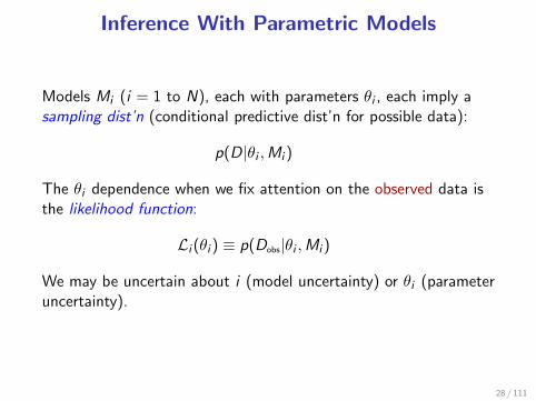
Inference With Parametric Models

Models Mi (i = 1 to N), each with parameters θi , each imply asampling dist’n (conditional predictive dist’n for possible data):

p(D|θi ,Mi )

The θi dependence when we fix attention on the observed data isthe likelihood function:

Li (θi ) ≡ p(Dobs|θi ,Mi )

We may be uncertain about i (model uncertainty) or θi (parameteruncertainty).

28 / 111

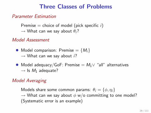
Three Classes of Problems

Parameter Estimation

Premise = choice of model (pick specific i)→ What can we say about θi?

Model Assessment

• Model comparison: Premise = Mi→ What can we say about i?

• Model adequacy/GoF: Premise = M1∨ “all” alternatives→ Is M1 adequate?

Model Averaging

Models share some common params: θi = φ, ηi→ What can we say about φ w/o committing to one model?(Systematic error is an example)

29 / 111

Parameter Estimation

Problem statement

I = Model M with parameters θ (+ any add’l info)Hi = statements about θ; e.g. “θ ∈ [2.5, 3.5],” or “θ > 0”Probability for any such statement can be found using aprobability density function (PDF) for θ:

P(θ ∈ [θ, θ + dθ]| · · · ) = f (θ)dθ

= p(θ| · · · )dθ

Posterior probability density

p(θ|D,M) =p(θ|M) L(θ)∫dθ p(θ|M) L(θ)

30 / 111

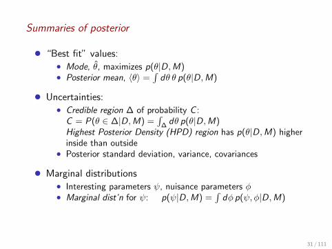
Summaries of posterior

• “Best fit” values:• Mode, θ, maximizes p(θ|D,M)• Posterior mean, 〈θ〉 =

∫dθ θ p(θ|D,M)

• Uncertainties:• Credible region ∆ of probability C :

C = P(θ ∈ ∆|D,M) =∫∆

dθ p(θ|D,M)Highest Posterior Density (HPD) region has p(θ|D,M) higherinside than outside

• Posterior standard deviation, variance, covariances

• Marginal distributions• Interesting parameters ψ, nuisance parameters φ• Marginal dist’n for ψ: p(ψ|D,M) =

∫dφ p(ψ, φ|D,M)

31 / 111

Nuisance Parameters and Marginalization

To model most data, we need to introduce parameters besidesthose of ultimate interest: nuisance parameters.

Example

We have data from measuring a rate r = s + b that is a sumof an interesting signal s and a background b.We have additional data just about b.What do the data tell us about s?

32 / 111

Marginal posterior distribution

p(s|D,M) =

∫db p(s, b|D,M)

∝ p(s|M)

∫db p(b|s)L(s, b)

≡ p(s|M)Lm(s)

with Lm(s) the marginal likelihood for s. For broad prior,

Lm(s) ≈ p(bs |s) L(s, bs) δbs

best b given s

b uncertainty given s

Profile likelihood Lp(s) ≡ L(s, bs) gets weighted by a parameterspace volume factor

E.g., Gaussians: s = r − b, σ2s = σ2

r + σ2b

Background subtraction is a special case of background marginalization.33 / 111

Model Comparison

Problem statement

I = (M1 ∨ M2 ∨ . . .) — Specify a set of models.Hi = Mi — Hypothesis chooses a model.

Posterior probability for a model

p(Mi |D, I ) = p(Mi |I )p(D|Mi , I )

p(D|I )∝ p(Mi |I )L(Mi )

But L(Mi ) = p(D|Mi ) =∫

dθi p(θi |Mi )p(D|θi ,Mi ).

Likelihood for model = Average likelihood for its parametersL(Mi ) = 〈L(θi )〉

Varied terminology: Prior predictive = Average likelihood = Globallikelihood = Marginal likelihood = (Weight of) Evidence for model

34 / 111

Odds and Bayes factors

A ratio of probabilities for two propositions using the samepremises is called the odds favoring one over the other:

Oij ≡ p(Mi |D, I )p(Mj |D, I )

=p(Mi |I )p(Mj |I )

× p(D|Mj , I )

p(D|Mj , I )

The data-dependent part is called the Bayes factor:

Bij ≡p(D|Mj , I )

p(D|Mj , I )

It is a likelihood ratio; the BF terminology is usually reserved forcases when the likelihoods are marginal/average likelihoods.

35 / 111

An Automatic Occam’s Razor

Predictive probabilities can favor simpler models

p(D|Mi ) =

∫dθi p(θi |M) L(θi )

DobsD

P(D|H)

Complicated H

Simple H

36 / 111

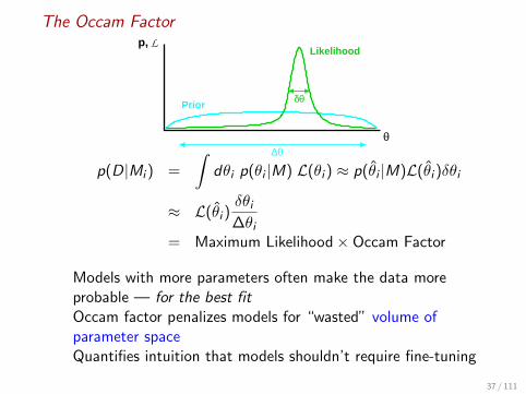
The Occam Factorp, L

θ∆θ

δθPrior

Likelihood

p(D|Mi ) =

∫dθi p(θi |M) L(θi ) ≈ p(θi |M)L(θi )δθi

≈ L(θi )δθi∆θi

= Maximum Likelihood × Occam Factor

Models with more parameters often make the data moreprobable — for the best fitOccam factor penalizes models for “wasted” volume ofparameter spaceQuantifies intuition that models shouldn’t require fine-tuning

37 / 111

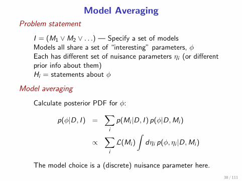
Model Averaging

Problem statement

I = (M1 ∨ M2 ∨ . . .) — Specify a set of modelsModels all share a set of “interesting” parameters, φEach has different set of nuisance parameters ηi (or differentprior info about them)Hi = statements about φ

Model averaging

Calculate posterior PDF for φ:

p(φ|D, I ) =∑

i

p(Mi |D, I ) p(φ|D,Mi )

∝∑

i

L(Mi )

∫dηi p(φ, ηi |D,Mi )

The model choice is a (discrete) nuisance parameter here.

38 / 111

Theme: Parameter Space Volume

Bayesian calculations sum/integrate over parameter/hypothesisspace!

(Frequentist calculations average over sample space & typically optimize

over parameter space.)

• Marginalization weights the profile likelihood by a volumefactor for the nuisance parameters.

• Model likelihoods have Occam factors resulting fromparameter space volume factors.

Many virtues of Bayesian methods can be attributed to thisaccounting for the “size” of parameter space. This idea does notarise naturally in frequentist statistics (but it can be added “byhand”).

39 / 111

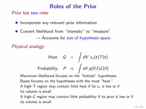
Roles of the PriorPrior has two roles

• Incorporate any relevant prior information

• Convert likelihood from “intensity” to “measure”

→ Accounts for size of hypothesis space

Physical analogy

Heat: Q =

∫dV cv (r)T (r)

Probability: P ∝∫

dθ p(θ|I )L(θ)

Maximum likelihood focuses on the “hottest” hypotheses.

Bayes focuses on the hypotheses with the most “heat.”

A high-T region may contain little heat if its cv is low or if

its volume is small.

A high-L region may contain little probability if its prior is low or if

its volume is small.40 / 111

Recap of Key Ideas

• Probability as generalized logic for appraising arguments

• Three theorems: BT, LTP, Normalization

• Calculations characterized by parameter space integrals• Credible regions, posterior expectations• Marginalization over nuisance parameters• Occam’s razor via marginal likelihoods

41 / 111









42 / 111

Binary Outcomes:Parameter Estimation

M = Existence of two outcomes, S and F ; each trial has sameprobability for S or F

Hi = Statements about α, the probability for success on the nexttrial → seek p(α|D,M)

D = Sequence of results from N observed trials:

FFSSSSFSSSFS (n = 8 successes in N = 12 trials)

Likelihood:

p(D|α,M) = p(failure|α,M) × p(success|α,M) × · · ·= αn(1 − α)N−n

= L(α)

43 / 111

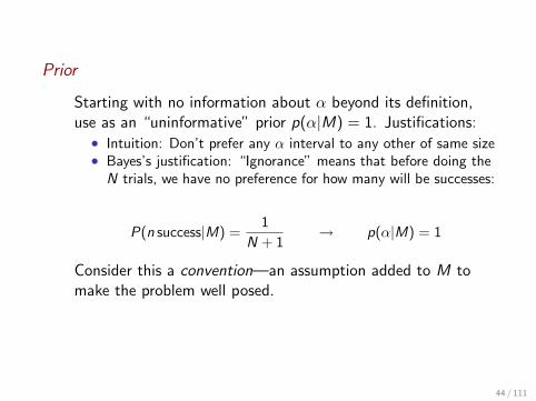
Prior

Starting with no information about α beyond its definition,use as an “uninformative” prior p(α|M) = 1. Justifications:

• Intuition: Don’t prefer any α interval to any other of same size• Bayes’s justification: “Ignorance” means that before doing the

N trials, we have no preference for how many will be successes:

P(n success|M) =1

N + 1→ p(α|M) = 1

Consider this a convention—an assumption added to M tomake the problem well posed.

44 / 111

Prior Predictive

p(D|M) =

∫dα αn(1 − α)N−n

= B(n + 1,N − n + 1) =n!(N − n)!

(N + 1)!

A Beta integral, B(a, b) ≡∫

dx xa−1(1 − x)b−1 = Γ(a)Γ(b)Γ(a+b) .

45 / 111

Posterior

p(α|D,M) =(N + 1)!

n!(N − n)!αn(1 − α)N−n

A Beta distribution. Summaries:

• Best-fit: α = nN

= 2/3; 〈α〉 = n+1N+2 ≈ 0.64

• Uncertainty: σα =√

(n+1)(N−n+1)(N+2)2(N+3)

≈ 0.12

Find credible regions numerically, or with incomplete betafunction

Note that the posterior depends on the data only through n,not the N binary numbers describing the sequence.n is a (minimal) Sufficient Statistic.

46 / 111

47 / 111

Binary Outcomes: Model ComparisonEqual Probabilities?

M1: α = 1/2M2: α ∈ [0, 1] with flat prior.

Maximum Likelihoods

M1 : p(D|M1) =1

2N= 2.44 × 10−4

M2 : L(α) =

(2

3

)n (1

3

)N−n

= 4.82 × 10−4

p(D|M1)

p(D|α,M2)= 0.51

Maximum likelihoods favor M2 (failures more probable).

48 / 111

Bayes Factor (ratio of model likelihoods)

p(D|M1) =1

2N; and p(D|M2) =

n!(N − n)!

(N + 1)!

→ B12 ≡ p(D|M1)

p(D|M2)=

(N + 1)!

n!(N − n)!2N

= 1.57

Bayes factor (odds) favors M1 (equiprobable).

Note that for n = 6, B12 = 2.93; for this small amount ofdata, we can never be very sure results are equiprobable.

If n = 0, B12 ≈ 1/315; if n = 2, B12 ≈ 1/4.8; for extremedata, 12 flips can be enough to lead us to strongly suspectoutcomes have different probabilities.

(Frequentist significance tests can reject null for any sample size.)

49 / 111

Binary Outcomes: Binomial DistributionSuppose D = n (number of heads in N trials), rather than theactual sequence. What is p(α|n,M)?

Likelihood

Let S = a sequence of flips with n heads.

p(n|α,M) =∑

Sp(S |α,M) p(n|S, α,M)

αn (1 − α)N−n

[ # successes = n]

= αn(1 − α)N−nCn,N

Cn,N = # of sequences of length N with n heads.

→ p(n|α,M) =N!

n!(N − n)!αn(1 − α)N−n

The binomial distribution for n given α, N.50 / 111

Posterior

p(α|n,M) =

N!n!(N−n)!α

n(1 − α)N−n

p(n|M)

p(n|M) =N!

n!(N − n)!


=1

N + 1

→ p(α|n,M) =(N + 1)!

n!(N − n)!αn(1 − α)N−n

Same result as when data specified the actual sequence.

51 / 111

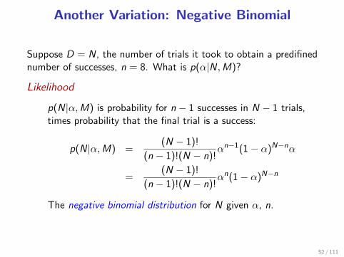
Another Variation: Negative Binomial

Suppose D = N, the number of trials it took to obtain a predifinednumber of successes, n = 8. What is p(α|N,M)?

Likelihood

p(N|α,M) is probability for n − 1 successes in N − 1 trials,times probability that the final trial is a success:

p(N|α,M) =(N − 1)!

(n − 1)!(N − n)!αn−1(1 − α)N−nα

=(N − 1)!

(n − 1)!(N − n)!αn(1 − α)N−n

The negative binomial distribution for N given α, n.

52 / 111

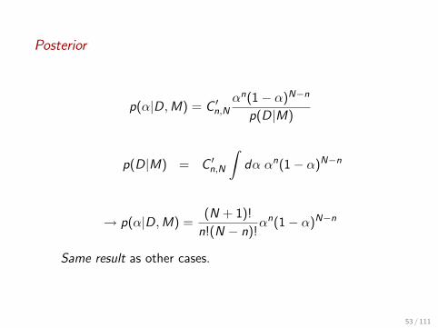
Posterior

p(α|D,M) = C ′n,N

αn(1 − α)N−n

p(D|M)

p(D|M) = C ′n,N


→ p(α|D,M) =(N + 1)!

n!(N − n)!αn(1 − α)N−n

Same result as other cases.

53 / 111

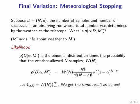
Final Variation: Meteorological Stopping

Suppose D = (N, n), the number of samples and number ofsuccesses in an observing run whose total number was determinedby the weather at the telescope. What is p(α|D,M ′)?

(M ′ adds info about weather to M.)

Likelihood

p(D|α,M ′) is the binomial distribution times the probabilitythat the weather allowed N samples, W (N):

p(D|α,M ′) = W (N)N!

n!(N − n)!αn(1 − α)N−n

Let Cn,N = W (N)(Nn

). We get the same result as before!

54 / 111

Likelihood Principle

To define L(Hi ) = p(Dobs|Hi , I ), we must contemplate what otherdata we might have obtained. But the “real” sample space may bedetermined by many complicated, seemingly irrelevant factors; itmay not be well-specified at all. Should this concern us?

Likelihood principle: The result of inferences depends only on howp(Dobs|Hi , I ) varies w.r.t. hypotheses. We can ignore aspects of theobserving/sampling procedure that do not affect this dependence.

This is a sensible property that frequentist methods do not share.Frequentist probabilities are “long run” rates of performance, anddepend on details of the sample space that are irrelevant in aBayesian calculation.

Example: Predict 10% of sample is Type A; observe nA = 5 for N = 96Significance test accepts α = 0.1 for binomial sampling;

p(> χ2|α = 0.1) = 0.12Significance test rejects α = 0.1 for negative binomial sampling;

p(> χ2|α = 0.1) = 0.0355 / 111

Inference With Normals/Gaussians

Gaussian PDF

p(x |µ, σ) =1

σ√

2πe−

(x−µ)2

2σ2 over [−∞,∞]

Common abbreviated notation: x ∼ N(µ, σ2)

Parameters

µ = 〈x〉 ≡∫

dx x p(x |µ, σ)

σ2 = 〈(x − µ)2〉 ≡∫

dx (x − µ)2 p(x |µ, σ)

56 / 111

Gauss’s Observation: Sufficiency

Suppose our data consist of N measurements, di = µ+ ǫi .Suppose the noise contributions are independent, andǫi ∼ N(0, σ2).

p(D|µ, σ,M) =∏

i

p(di |µ, σ,M)

=∏

i

p(ǫi = di − µ|µ, σ,M)

=∏

i

1

σ√

2πexp

[−(di − µ)2

2σ2

]

=1

σN(2π)N/2e−Q(µ)/2σ2

57 / 111

Find dependence of Q on µ by completing the square:

Q =∑

i

(di − µ)2

=∑

i

d2i + Nµ2 − 2Nµd where d ≡ 1

N

∑

i

di

= N(µ− d)2 + Nr2 where r2 ≡ 1

N

∑

i

(di − d)2

Likelihood depends on di only through d and r :

L(µ, σ) =1

σN(2π)N/2exp

(−Nr2

2σ2

)exp

(−N(µ− d)2

2σ2

)

The sample mean and variance are sufficient statistics.

This is a miraculous compression of information—the normal dist’nis highly abnormal in this respect!

58 / 111

Estimating a Normal Mean

Problem specification

Model: di = µ+ ǫi , ǫi ∼ N(0, σ2), σ is known → I = (σ,M).Parameter space: µ; seek p(µ|D, σ,M)

Likelihood

p(D|µ, σ,M) =1

σN(2π)N/2exp

(−Nr2

2σ2

)exp

(−N(µ− d)2

2σ2

)

∝ exp

(−N(µ− d)2

2σ2

)

59 / 111

“Uninformative” prior

Translation invariance ⇒ p(µ) ∝ C , a constant.This prior is improper unless bounded.

Prior predictive/normalization

p(D|σ,M) =

∫dµ C exp

(−N(µ− d)2

2σ2

)

= C (σ/√

N)√

2π

. . . minus a tiny bit from tails, using a proper prior.

60 / 111

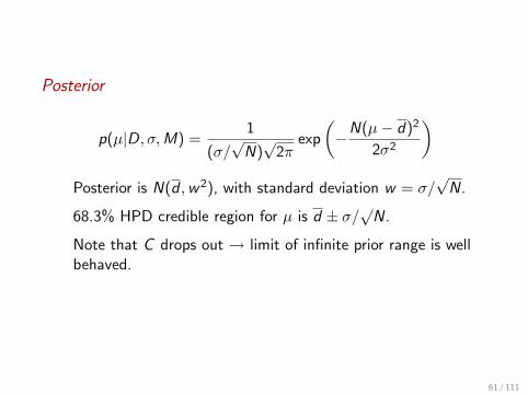
Posterior

p(µ|D, σ,M) =1

(σ/√

N)√

2πexp

(−N(µ− d)2

2σ2

)

Posterior is N(d ,w2), with standard deviation w = σ/√

N.

68.3% HPD credible region for µ is d ± σ/√

N.

Note that C drops out → limit of infinite prior range is wellbehaved.

61 / 111

Informative Conjugate Prior

Use a normal prior, µ ∼ N(µ0,w20 )

Posterior

Normal N(µ, w2), but mean, std. deviation “shrink” towardsprior.Define B = w2

w2+w20, so B < 1 and B = 0 when w0 is large.

Then

µ = (1 − B) · d + B · µ0

w = w ·√

1 − B

“Principle of stable estimation:” The prior affects estimatesonly when data are not informative relative to prior.

62 / 111

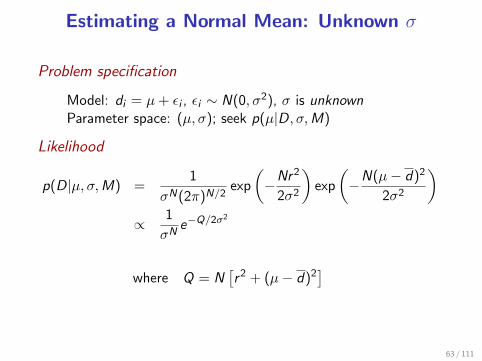
Estimating a Normal Mean: Unknown σ

Problem specification

Model: di = µ+ ǫi , ǫi ∼ N(0, σ2), σ is unknownParameter space: (µ, σ); seek p(µ|D, σ,M)

Likelihood

p(D|µ, σ,M) =1

σN(2π)N/2exp

(−Nr2

2σ2

)exp

(−N(µ− d)2

2σ2

)

∝ 1

σNe−Q/2σ2

where Q = N[r2 + (µ− d)2

]

63 / 111

Uninformative Priors

Assume priors for µ and σ are independent.Translation invariance ⇒ p(µ) ∝ C , a constant.Scale invariance ⇒ p(σ) ∝ 1/σ (flat in log σ).

Joint Posterior for µ, σ

p(µ, σ|D,M) ∝ 1

σN+1e−Q(µ)/2σ2

64 / 111

Marginal Posterior

p(µ|D,M) ∝∫

dσ1

σN+1e−Q/2σ2

Let τ = Q2σ2 so σ =

√Q2τ and |dσ| = τ−3/2

√Q2

⇒ p(µ|D,M) ∝ 2N/2Q−N/2

∫dτ τ

N2−1e−τ

∝ Q−N/2

65 / 111

Write Q = Nr2

[1 +

(µ−d

r

)2]

and normalize:

p(µ|D,M) =

(N2 − 1

)!(

N2 − 3

2

)!√π

1

r

[1 +

1

N

(µ− d

r/√

N

)2]−N/2

“Student’s t distribution,” with t = (µ−d)

r/√

N

A “bell curve,” but with power-law tailsLarge N:

p(µ|D,M) ∼ e−N(µ−d)2/2r2

66 / 111

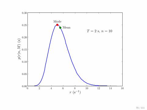
Poisson Dist’n: Infer a Rate from Counts

Problem: Observe n counts in T ; infer rate, r

Likelihood

L(r) ≡ p(n|r ,M) = p(n|r ,M) =(rT )n

n!e−rT

Prior

Two simple standard choices (or conjugate gamma dist’n):

• r known to be nonzero; it is a scale parameter:

p(r |M) =1

ln(ru/rl)

1

r

• r may vanish; require p(n|M) ∼ Const:

p(r |M) =1

ru

67 / 111

Prior predictive

p(n|M) =1

ru

1

n!

∫ ru

0dr(rT )ne−rT

=1

ruT

1

n!

∫ ruT

0d(rT )(rT )ne−rT

≈ 1

ruTfor ru ≫ n

T

Posterior

A gamma distribution:

p(r |n,M) =T (rT )n

n!e−rT

68 / 111

Gamma Distributions

A 2-parameter family of distributions over nonnegative x , withshape parameter α and scale parameter s:

pΓ(x |α, s) =1

sΓ(α)

(x

s

)α−1e−x/s

Moments:

E(x) = sν Var(x) = s2ν

Our posterior corresponds to α = n + 1, s = 1/T .

• Mode r = nT

; mean 〈r〉 = n+1T

(shift down 1 with 1/r prior)

• Std. dev’n σr =√

n+1T

; credible regions found by integrating (canuse incomplete gamma function)

69 / 111

70 / 111

The flat prior

Bayes’s justification: Not that ignorance of r → p(r |I ) = CRequire (discrete) predictive distribution to be flat:

p(n|I ) =

∫dr p(r |I )p(n|r , I ) = C

→ p(r |I ) = C

Useful conventions

• Use a flat prior for a rate that may be zero

• Use a log-flat prior (∝ 1/r) for a nonzero scale parameter

• Use proper (normalized, bounded) priors

• Plot posterior with abscissa that makes prior flat

71 / 111

The On/Off Problem

Basic problem

• Look off-source; unknown background rate bCount Noff photons in interval Toff

• Look on-source; rate is r = s + b with unknown signal sCount Non photons in interval Ton

• Infer s

Conventional solution

b = Noff/Toff ; σb =√

Noff/Toff

r = Non/Ton; σr =√

Non/Ton

s = r − b; σs =√σ2

r + σ2b

But s can be negative!

72 / 111

Examples

Spectra of X-Ray Sources

Bassani et al. 1989 Di Salvo et al. 2001

73 / 111

Spectrum of Ultrahigh-Energy Cosmic Rays

Nagano & Watson 2000

HiRes Team 2007

log10(E) (eV)F

lux*

E3 /1

024 (

eV2 m

-2 s

-1 s

r-1)

AGASAHiRes-1 MonocularHiRes-2 Monocular

1

10

17 17.5 18 18.5 19 19.5 20 20.5 21

74 / 111

N is Never Large

“Sample sizes are never large. If N is too small to get asufficiently-precise estimate, you need to get more data (or makemore assumptions). But once N is ‘large enough,’ you can startsubdividing the data to learn more (for example, in a publicopinion poll, once you have a good estimate for the entire country,you can estimate among men and women, northerners andsoutherners, different age groups, etc etc). N is never enoughbecause if it were ‘enough’ you’d already be on to the nextproblem for which you need more data.

“Similarly, you never have quite enough money. But that’s anotherstory.”

— Andrew Gelman (blog entry, 31 July 2005)

75 / 111

Backgrounds as Nuisance Parameters

Background marginalization with Gaussian noise

Measure background rate b = b ± σb with source off. Measure total

rate r = r ± σr with source on. Infer signal source strength s, where

r = s + b. With flat priors,

p(s, b|D,M) ∝ exp

[− (b − b)2

2σ2b

]× exp

[− (s + b − r)2

2σ2r

]

76 / 111

Marginalize b to summarize the results for s (complete thesquare to isolate b dependence; then do a simple Gaussianintegral over b):

p(s|D,M) ∝ exp

[−(s − s)2

2σ2s

]s = r − bσ2

s = σ2r + σ2

b

⇒ Background subtraction is a special case of backgroundmarginalization.

77 / 111

Bayesian Solution to On/Off Problem

First consider off-source data; use it to estimate b:

p(b|Noff , Ioff) =Toff(bToff)Noff e−bToff

Noff !

Use this as a prior for b to analyze on-source data. For on-sourceanalysis Iall = (Ion,Noff , Ioff):

p(s, b|Non) ∝ p(s)p(b)[(s + b)Ton]None−(s+b)Ton || Iall

p(s|Iall) is flat, but p(b|Iall) = p(b|Noff , Ioff), so

p(s, b|Non, Iall) ∝ (s + b)NonbNoff e−sTone−b(Ton+Toff)

78 / 111

Now marginalize over b;

p(s|Non, Iall) =

∫db p(s, b | Non, Iall)

∝∫

db (s + b)NonbNoff e−sTone−b(Ton+Toff)

Expand (s + b)Non and do the resulting Γ integrals:

p(s|Non, Iall) =

Non∑

i=0

Ci

Ton(sTon)ie−sTon

i !

Ci ∝(

1 +Toff

Ton

)i(Non + Noff − i)!

(Non − i)!

Posterior is a weighted sum of Gamma distributions, each assigning adifferent number of on-source counts to the source. (Evaluate viarecursive algorithm or confluent hypergeometric function.)

79 / 111

Example On/Off Posteriors—Short Integrations

Ton = 1

80 / 111

Example On/Off Posteriors—Long Background Integrations

Ton = 1

81 / 111









82 / 111

Empirical Number Counts DistributionsStar counts, galaxy counts, GRBs, TNOs . . .

BATSE 4B Catalog (≈ 1200 GRBs)

F ∝ L/d2 [× cosmo, extinct’n]

13 TNO Surveys (c. 2001)

F ∝ νD2/(d2⊙d2

⊕)

83 / 111

Selection Effects and Measurement Error

• Selection effects (truncation, censoring) — obvious (usually)Typically treated by “correcting” dataMost sophisticated: product-limit estimators

• “Scatter” effects (measurement error, etc.) — insidiousTypically ignored (average out?)

84 / 111

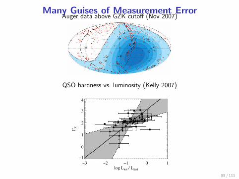
Many Guises of Measurement ErrorAuger data above GZK cutoff (Nov 2007)

QSO hardness vs. luminosity (Kelly 2007)

85 / 111

History

Eddington, Jeffreys (1920s – 1940)

n

m

n

m

m Uncertainty

^

Malmquist, Lutz-Kelker

• Joint accounting for truncation and (intrinsic) scatter in 2-Ddata (flux + distance indicator, parallax)

• Assume homogeneous spatial distribution

86 / 111

Many rediscoveries of “scatter biases”

• Radio sources (1970s)

• Galaxies (Eddington, Malmquist; 1990s)

• Linear regression (1990s)

• GRBs (1990s)

• X-ray sources (1990s; 2000s)

• TNOs/KBOs (c. 2000)

• Galaxy redshift dist’ns (2007+)

• · · ·

87 / 111

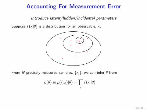
Accounting For Measurement Error

Introduce latent/hidden/incidental parameters

Suppose f (x |θ) is a distribution for an observable, x .

From N precisely measured samples, xi, we can infer θ from

L(θ) ≡ p(xi|θ) =∏

i

f (xi |θ)

88 / 111

Graphical representation

θ

x1 x2 xN

L(θ) ≡ p(xi|θ) =∏

i

f (xi |θ)

89 / 111

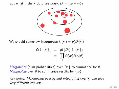
But what if the x data are noisy, Di = xi + ǫi?

We should somehow incorporate ℓi (xi ) = p(Di |xi )

L(θ, xi) ≡ p(Di|θ, xi)=

∏

i

ℓi (xi )f (xi |θ)

Marginalize (sum probabilities) over xi to summarize for θ.Marginalize over θ to summarize results for xi.

Key point: Maximizing over xi and integrating over xi can givevery different results!

90 / 111

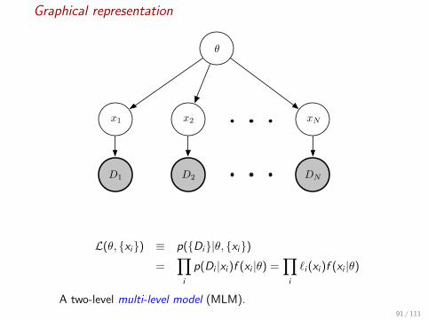
Graphical representation

DND1 D2

θ

x1 x2 xN

L(θ, xi) ≡ p(Di|θ, xi)=

∏

i

p(Di |xi )f (xi |θ) =∏

i

ℓi (xi )f (xi |θ)

A two-level multi-level model (MLM).91 / 111

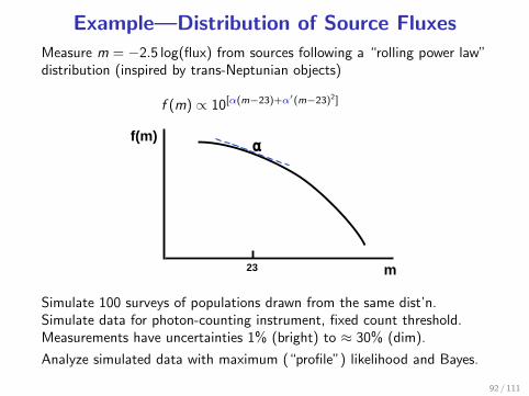
Example—Distribution of Source Fluxes

Measure m = −2.5 log(flux) from sources following a “rolling power law”distribution (inspired by trans-Neptunian objects)

f (m) ∝ 10[α(m−23)+α′(m−23)2]

m

f(m)

23

α

Simulate 100 surveys of populations drawn from the same dist’n.Simulate data for photon-counting instrument, fixed count threshold.Measurements have uncertainties 1% (bright) to ≈ 30% (dim).

Analyze simulated data with maximum (“profile”) likelihood and Bayes.

92 / 111

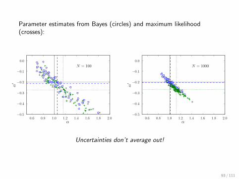
Parameter estimates from Bayes (circles) and maximum likelihood(crosses):

Uncertainties don’t average out!

93 / 111

Smaller measurement error only postpones the inevitable:

Similar toy survey, with parameters to mimic SDSS QSO surveys (few %errors at dim end):

94 / 111

Bayesian MLMs in Astronomy

• Directional & spatio-temporal coincidences:

• GRB repetition (Luo+ 1996; Graziani+ 1996)

• GRB host ID (Band 1998; Graziani+ 1999)

• VO cross-matching (Badav/’ari & Szalay 2008)

• Magnitude surveys/number counts/“log N–log S”:

• GRB peak flux dist’n (Loredo & Wasserman 1998);

• TNO/KBO magnitude distribution (Gladman+ 1998;Petit+ 2008)

• Dynamic spectroscopy: SN 1987A neutrinos, uncertainenergy vs. time (Loredo & Lamb 2002)

• Linear regression: QSO hardness vs. luminosity (Kelly 2007)

95 / 111









96 / 111

Bayesian Computation

Large sample size: Laplace approximation

• Approximate posterior as multivariate normal → det(covar) factors• Uses ingredients available in χ2/ML fitting software (MLE, Hessian)• Often accurate to O(1/N)

Low-dimensional models (d<∼10 to 20)

• Adaptive cubature• Monte Carlo integration (importance sampling, quasirandom MC)

Hi-dimensional models (d>∼5)

• Posterior sampling—create RNG that samples posterior• MCMC is most general framework

97 / 111









98 / 111

Probability & Frequency

Frequencies are relevant when modeling repeated trials, orrepeated sampling from a population or ensemble.

Frequencies are observables:

• When available, can be used to infer probabilities for next trial

• When unavailable, can be predicted

Bayesian/Frequentist relationships:

• General relationships between probability and frequency

• Long-run performance of Bayesian procedures

• Examples of Bayesian/frequentist differences

99 / 111

Relationships Between Probability & Frequency

Frequency from probability

Bernoulli’s law of large numbers: In repeated i.i.d. trials, givenP(success| . . .) = α, predict

Nsuccess

Ntotal

→ α as Ntotal → ∞

Probability from frequency

Bayes’s “An Essay Towards Solving a Problem in the Doctrineof Chances” → First use of Bayes’s theorem:Probability for success in next trial of i.i.d. sequence:

Eα→ Nsuccess

Ntotal

as Ntotal → ∞

100 / 111

Subtle Relationships For Non-IID CasesPredict frequency in dependent trials

rt = result of trial t; p(r1, r2 . . . rN |M) known; predict f :

〈f 〉 =1

N

∑

t

p(rt = success|M)

where p(r1|M) =∑

r2

· · ·∑

rN

p(r1, r2 . . . |M3)

Expected frequency of outcome in many trials =average probability for outcome across trials.But also find that σf needn’t converge to 0.

Infer probabilities for different but related trialsShrinkage: Biased estimators of the probability that share infoacross trials are better than unbiased/BLUE/MLE estimators.

A formalism that distinguishes p from f from the outset is particularlyvaluable for exploring subtle connections. E.g., shrinkage is explored viahierarchical and empirical Bayes.

101 / 111

Frequentist Performance of Bayesian Procedures

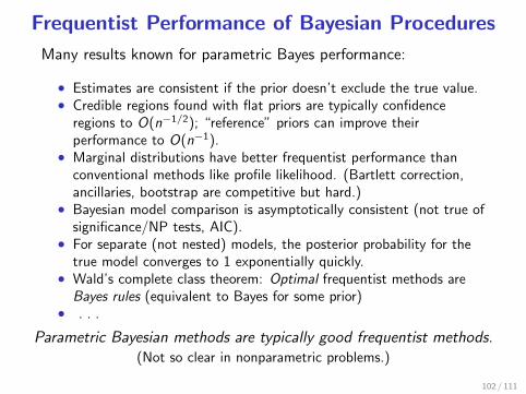
Many results known for parametric Bayes performance:

• Estimates are consistent if the prior doesn’t exclude the true value.• Credible regions found with flat priors are typically confidence

regions to O(n−1/2); “reference” priors can improve theirperformance to O(n−1).

• Marginal distributions have better frequentist performance thanconventional methods like profile likelihood. (Bartlett correction,ancillaries, bootstrap are competitive but hard.)

• Bayesian model comparison is asymptotically consistent (not true ofsignificance/NP tests, AIC).

• For separate (not nested) models, the posterior probability for thetrue model converges to 1 exponentially quickly.

• Wald’s complete class theorem: Optimal frequentist methods areBayes rules (equivalent to Bayes for some prior)

• . . .

Parametric Bayesian methods are typically good frequentist methods.(Not so clear in nonparametric problems.)

102 / 111









103 / 111

Some Bayesian Astrostatistics Hotspots

• Cosmology• Parametric modeling of CMB, LSS, SNe Ia → cosmo params• Nonparametric modeling of SN Ia multicolor light curves• Nonparametric “emulation” of cosmological models

• Extrasolar planets• Parametric modeling of Keplerian reflex motion (planet

detection, orbit estimation)• Optimal scheduling via Bayesian experimental design

• Photon counting data (X-rays, γ-rays, cosmic rays)• Upper limits, hardness ratios• Parametric spectroscopy (line detection, etc.)

• Gravitational wave astronomy• Parametric modeling of binary inspirals• Hi-multiplicity parametric modeling of white dwarf background

104 / 111

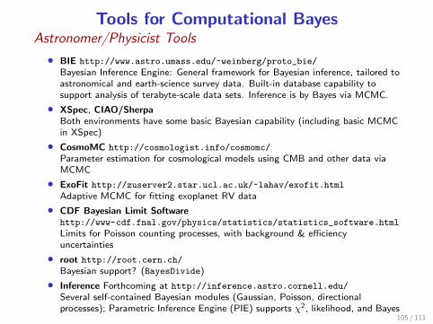
Tools for Computational BayesAstronomer/Physicist Tools

• BIE http://www.astro.umass.edu/~weinberg/proto_bie/

Bayesian Inference Engine: General framework for Bayesian inference, tailored toastronomical and earth-science survey data. Built-in database capability tosupport analysis of terabyte-scale data sets. Inference is by Bayes via MCMC.

• XSpec, CIAO/SherpaBoth environments have some basic Bayesian capability (including basic MCMCin XSpec)

• CosmoMC http://cosmologist.info/cosmomc/

Parameter estimation for cosmological models using CMB and other data viaMCMC

• ExoFit http://zuserver2.star.ucl.ac.uk/~lahav/exofit.html

Adaptive MCMC for fitting exoplanet RV data

• CDF Bayesian Limit Softwarehttp://www-cdf.fnal.gov/physics/statistics/statistics_software.html

Limits for Poisson counting processes, with background & efficiencyuncertainties

• root http://root.cern.ch/

Bayesian support? (BayesDivide)

• Inference Forthcoming at http://inference.astro.cornell.edu/Several self-contained Bayesian modules (Gaussian, Poisson, directionalprocesses); Parametric Inference Engine (PIE) supports χ2, likelihood, and Bayes

105 / 111

http://www.astro.umass.edu/~weinberg/proto_bie/

http://cosmologist.info/cosmomc/

http://zuserver2.star.ucl.ac.uk/~lahav/exofit.html

http://www-cdf.fnal.gov/physics/statistics/statistics_software.html

http://root.cern.ch/

http://inference.astro.cornell.edu/

Python

• PyMC http://trichech.us/pymc

A framework for MCMC via Metropolis-Hastings; also implements Kalmanfilters and Gaussian processes. Targets biometrics, but is general.

• SimPy http://simpy.sourceforge.net/

Intro to SimPy http://heather.cs.ucdavis.edu/ matloff/simpy.html SimPy(rhymes with ”Blimpie”) is a process-oriented public-domain package fordiscrete-event simulation.

• RSPython http://www.omegahat.org/

Bi-directional communication between Python and R

• MDP http://mdp-toolkit.sourceforge.net/

Modular toolkit for Data Processing: Current emphasis is on machine learning(PCA, ICA. . . ). Modularity allows combination of algorithms and other dataprocessing elements into “flows.”

• Orange http://www.ailab.si/orange/

Component-based data mining, with preprocessing, modeling, and explorationcomponents. Python/GUI interfaces to C + + implementations. Some Bayesiancomponents.

• ELEFANT http://rubis.rsise.anu.edu.au/elefant

Machine learning library and platform providing Python interfaces to efficient,lower-level implementations. Some Bayesian components (Gaussian processes;Bayesian ICA/PCA).

106 / 111

http://trichech.us/pymc

http://simpy.sourceforge.net/

http://www.omegahat.org/

http://mdp-toolkit.sourceforge.net/

http://www.ailab.si/orange/

http://rubis.rsise.anu.edu.au/elefant

R and S

• CRAN Bayesian task viewhttp://cran.r-project.org/src/contrib/Views/Bayesian.html

Overview of many R packages implementing various Bayesian models andmethods

• Omega-hat http://www.omegahat.org/

RPython, RMatlab, R-Xlisp

• BOA http://www.public-health.uiowa.edu/boa/

Bayesian Output Analysis: Convergence diagnostics and statistical and graphicalanalysis of MCMC output; can read BUGS output files.

• CODAhttp://www.mrc-bsu.cam.ac.uk/bugs/documentation/coda03/cdaman03.html

Convergence Diagnosis and Output Analysis: Menu-driven R/S plugins foranalyzing BUGS output

107 / 111

http://cran.r-project.org/src/contrib/Views/Bayesian.html


http://www.public-health.uiowa.edu/boa/

http://www.mrc-bsu.cam.ac.uk/bugs/documentation/coda03/cdaman03.html

Java

• Omega-hat http://www.omegahat.org/

Java environment for statistical computing, being developed by XLisp-stat andR developers

• Hydra http://research.warnes.net/projects/mcmc/hydra/

HYDRA provides methods for implementing MCMC samplers using Metropolis,Metropolis-Hastings, Gibbs methods. In addition, it provides classesimplementing several unique adaptive and multiple chain/parallel MCMCmethods.

• YADAS http://www.stat.lanl.gov/yadas/home.html

Software system for statistical analysis using MCMC, based on themulti-parameter Metropolis-Hastings algorithm (rather thanparameter-at-a-time Gibbs sampling)

108 / 111


http://research.warnes.net/projects/mcmc/hydra/

http://www.stat.lanl.gov/yadas/home.html

C/C++/Fortran

• BayeSys 3 http://www.inference.phy.cam.ac.uk/bayesys/

Sophisticated suite of MCMC samplers including transdimensional capability, bythe author of MemSys

• fbm http://www.cs.utoronto.ca/~radford/fbm.software.html

Flexible Bayesian Modeling: MCMC for simple Bayes, Bayesian regression andclassification models based on neural networks and Gaussian processes, andBayesian density estimation and clustering using mixture models and Dirichletdiffusion trees

• BayesPack, DCUHREhttp://www.sci.wsu.edu/math/faculty/genz/homepage

Adaptive quadrature, randomized quadrature, Monte Carlo integration

• BIE, CDF Bayesian limits (see above)

109 / 111

http://www.inference.phy.cam.ac.uk/bayesys/

http://www.cs.utoronto.ca/~radford/fbm.software.html

http://www.sci.wsu.edu/math/faculty/genz/homepage

Other Statisticians’ & Engineers’ Tools

• BUGS/WinBUGS http://www.mrc-bsu.cam.ac.uk/bugs/

Bayesian Inference Using Gibbs Sampling: Flexible software for the Bayesiananalysis of complex statistical models using MCMC

• OpenBUGS http://mathstat.helsinki.fi/openbugs/

BUGS on Windows and Linux, and from inside the R

• XLisp-stat http://www.stat.uiowa.edu/~luke/xls/xlsinfo/xlsinfo.html

Lisp-based data analysis environment, with an emphasis on providing aframework for exploring the use of dynamic graphical methods

• ReBEL http://choosh.csee.ogi.edu/rebel/

Library supporting recursive Bayesian estimation in Matlab (Kalman filter,particle filters, sequential Monte Carlo).

110 / 111

http://www.mrc-bsu.cam.ac.uk/bugs/

http://mathstat.helsinki.fi/openbugs/

http://www.stat.uiowa.edu/~luke/xls/xlsinfo/xlsinfo.html

http://choosh.csee.ogi.edu/rebel/

Closing Reflections

Philip Dawid (2000)

What is the principal distinction between Bayesian and classical statistics? It isthat Bayesian statistics is fundamentally boring. There is so little to do: justspecify the model and the prior, and turn the Bayesian handle. There is noroom for clever tricks or an alphabetic cornucopia of definitions and optimalitycriteria. I have heard people use this ‘dullness’ as an argument againstBayesianism. One might as well complain that Newton’s dynamics, being basedon three simple laws of motion and one of gravitation, is a poor substitute forthe richness of Ptolemy’s epicyclic system.All my experience teaches me that it is invariably more fruitful, and leads todeeper insights and better data analyses, to explore the consequences of being a‘thoroughly boring Bayesian’.

Dennis Lindley (2000)

The philosophy places more emphasis on model construction than on formalinference. . . I do agree with Dawid that ‘Bayesian statistics is fundamentallyboring’. . .My only qualification would be that the theory may be boring but theapplications are exciting.

111 / 111

Documents

Tom Loredo Dept. of Astronomy, Cornell University http ...astrostatistics.psu.edu/su09/lecturenotes/bayesLoredo.pdf · Bayesian inference quantiﬁes uncertainty by reporting probabilities