Tom a s Horv ath BUSINESS ANALYTICS · s;tare the smoothed values of fin the corresponding spectrum s coe cients c s;trepresent the di erences in values of fin the corresponding spectrum

Tomas Horvath

BUSINESS ANALYTICS

Lecture 4

Time Series

Information Systems and Machine Learning Lab

University of Hildesheim

Germany

Overview

The aim of this lecture is to get insight to time series mining

• Representation of time series

• Distance measures

• Time series Classification

• Forecasting

Tomas Horvath ISMLL, University of Hildesheim, Germany 1/57

Univariate time series

A univariate time series x of length l is a sequencex = (x0, x1, . . . , xl−1), where xj ∈ R for each 0 ≤ j < l.

D = {(xi, c(xi))}ni=1 is a labeled time series dataset, where c : T → C isa mapping from the set T of time series to a set C of classes.


Raw Representation

Listing all the values is not necessary the most approppriate way,especially, when the aim is to classify time series.• classification algorithms deal with the features of instances

• approximate/condensed representations of time series are desirable• the patterns are usually most interesting than individual points


Different types of representation

Discrete Fourier1 Transform (DFT)

Haar Wavelet1 transformation (DHWT)

Piecewise Linear Approximation (PLA)

• interpolation

• regression

Piecewise Constant Approximation (PCA)

• Piecewise Aggregate Approximation (PAA)

• Adaptive Piecewise Constant Approximation (APCA)

Symbolic Aggregate Approximation (SAX)

1Just the basic definitions will be discussed here, since more detailed descriptions are out of the scope

of the lecture. See the references at the end of this presentation for more details.


Fourier Series

We can write a Fourier series of any continuous, differentiable andT-periodic1 function f : R→ C as

f(x) =a02

+

∞∑k=1

ak cos(kωx) + bk sin(kωx), ω =2π

T

with coefficients ak, bk ∈ C, such that

ak =1πω

+ πω∫

− πω

f(x) cos(kωx) dx

bk =1πω

+ πω∫

− πω

f(x) sin(kωx) dx

1A function f : R→ C is T-periodic if f(x + T ) = f(x) for each x ∈ R.


Fourier Series: Examplef(x) = −sin(x) + cos(x) + 8 sin(2x)− cos(2x) + 11 cos(3x)− 5 sin(5x) + 7 cos(5x)

f(x) = −sin(x) + cos(x)f(x) = −sin(x) + cos(x) + 8 sin(2x)− cos(2x)f(x) = −sin(x) + cos(x) + 8 sin(2x)− cos(2x) + 11 cos(3x)f(x) = −sin(x) + cos(x) + 8 sin(2x)− cos(2x) + 11 cos(3x)− 5 sin(5x) + 7 cos(5x)


Complex Fourier Series

Euler formulaeix = cos(x) + i · sin(x)

We can write a complex Fourier series of any continuous,differentiable and T-periodic function f : R→ C as

f(x) =∑k∈Z

ckeikωx, ω =

2π

T

with complex coefficients ck ∈ C, such that

ck =12πω

+ πω∫

− πω

f(x) e−ikωx dx


Fourier transform

A Fourier transform1 of a continuous, differentiable and T-periodicfunction f : R→ C is a mapping F : R→ C defined as

F (ω) =1√2π

+∞∫−∞

f(x) e−iωx dx

If F also satisfies some regularity conditions than we can define theinverze Fourier transform as

f(x) =1√2π

+∞∫−∞

F (ω) eiωx dω

1Called also as a Fourier spectrum of f


Discrete Fourier transform (DFT)

A Discrete Fourier transform Fd(f) of a finite, discrete functionf : {0, 1, . . . , n− 1} → C is a mapping Fd : {0, 1, . . . , n− 1} → Cdefined as

Fd(ω) =1√n

n−1∑x=0

f(x)(cos(2π

ωx

n)−i·sin(2π

ωx

n))

=1√n

n−1∑x=0

f(x)e−i2πωxn

An inverze discrete Fourier transform is defined as

f(x) =1√n

n−1∑ω=0

Fd(ω)(cos(2π

ωx

n)+i·sin(2π

ωx

n))

=1√n

n−1∑ω=0

Fd(ω)ei2πωxn


Computation of DFT

f(x) consists of real and imaginary parts

• f(x) = f(x)re + i · f(x)im ∈ C

Thus, we compute1 Fd(ω) for each ω ∈ {0, 1, . . . , n− 1} as

Fd(ω) = 1√n

n−1∑x=0

f(x)(cos(2π ωxn )− i · sin(2π ωxn )

)= 1√

n

n−1∑x=0

f(x)re cos(2πωxn ) + f(x)imsin(2π ωxn )

+ i · 1√n

n−1∑x=0−f(x)re sin(2π ωxn ) + f(x)imcos(2π

ωxn )

1An efficient way of computation called fast Fourier transform (FFT) can be found in the literature.

FFT works well for the sequences of even length, best for lengths of 2k, where k ∈ N.


DFT: Example (1)

Sample 16 points from the example before• f ′(x′) = −sin(x′) + cos(x′) + 8 sin(2x′)− cos(2x′) + 11 cos(3x′)− 5 sin(5x′) + 7 cos(5x′) for

x′ ∈ {−8, . . . ,−1, 1, . . . , 8}• f ′(−8) = 7.828, f ′(−1) = −19.175, . . . , f ′(1) = 3.280, . . . , f ′(8) = −6.209

x f(x)re f(x)im0 7.828 +0.000i1 -21.142 +0.000i2 7.533 +0.000i3 2.436 +0.000i4 7.524 +0.000i5 -11.663 +0.000i6 9.169 +0.000i7 -19.175 +0.000i8 3.280 +0.000i9 0.682 +0.000i

10 -22.918 +0.000i11 15.738 +0.000i12 -3.027 +0.000i13 9.387 +0.000i14 -2.325 +0.000i15 -6.209 +0.000i

DFT=⇒

ω Fd(ω)re Fd(ω)im0 -22.883 +0.000i1 12.733 +4.840i2 -37.048 +4.288i3 -19.404 -0.111i4 24.146 +15.526i5 1.691 +38.107i6 50.269 -40.172i7 23.171 +85.261i8 37.010 +0.000i9 23.171 -85.261i

10 50.269 +40.172i11 1.691 -38.107i12 24.146 -15.52613 -19.404 +0.111i14 -37.048 -4.288i15 12.733 -4.840i


DFT: Example (2)

Real and Imaginary parts of DFT on Australian Beer Production data


Haar wavelet and basis functions

The Haar wavelet ψ : R→ R isdefined as

ψ(x) =

+1, x ∈ 〈0, 12)−1, x ∈ 〈12 , 1)

0, else

Haar basis functions ψs,t : R→ R, s, t ∈ Z are defined as

ψs,t =√

2s · ψ(2sx− t) =√

2s ·

+1, x ∈ 〈2−st, 2−s(t+ 1

2))−1, x ∈ 〈2−s(t+ 1

2), 2−s(t+ 1))0, else


Haar basis functions: Example


Haar Wavelet representation

Every function f : R→ R satisfying some regularity conditions can bewritten as

f(x) =∑s∈Z

∑t∈Z

cs,t ψs,t(x)

with cs,t ∈ R, such that

cs,t =√

2s( 2−s(t+ 1

2)∫

2−st

f(x)dx−2−s(t+1)∫

2−s(t+ 12)

f(x)dx)

=1√2

(as+1,2t−as+1,2t+1)

where as,t can be computed recursively as

as,t =√

2s

2−s(t+1)∫2−st

f(x) dx =1√2

(as+1,2t + as+1,2t+1)


Discrete Haar Wavelet Transform (DHWT)

A finite, discrete function f : {0, 1, . . . , n− 1} → R, with lengthn = 2k, k ∈ N can be represented as

f(x) = a−n,0 +

−1∑s=−n

2n+s−1∑t=0

cs,t ·√

2s · ψs,t(x)

where the initial values a0,t are the original values of f , i.e. a0,t = f(t).

DHWT allows time series to be viewed in multiple resolutionscorresponding to frequencies or spectrums1

• coefficients as,t are the smoothed values of f in the correspondingspectrum s

• coefficients cs,t represent the differences in values of f in thecorresponding spectrum s

1Averages and differences are computed across a window of values.


DHWT: Example

t 0 1 2 3 4 5 6 7f(t) 1 3 5 4 8 2 -1 7

a−1,t4√2

9√2

10√2

6√2

– – – –

c−1,t−2√

21√2

6√2

−8√2

– – – –

a−2,t132

162

– – – – – –

c−2,t−52

42

– – – – – –

a−3,t29

2√

2– – – – – – –

c−3,t−3

2√

2– – – – – – –

(1, 3, 5, 4, 8, 2,−1, 7) ( 292√

2, −3

2√

2, −5

2, 42, −2√

2, 1√

2, 6√

2, −8√

2)


Piecewise Linear Approximation

Regression

Interpolation


PLA: Sliding Windows

Anchor a left point and approximate data to the right with increasingsize of a window while the error is under a given treshold


PLA: Top-down approach

Taking into account every possible partition split at the best locationrecursively while the error is above a given threshold


PLA: Bottom-up approach

Starting from the finest possible approximation merge segments whilethe error is above the given threshold


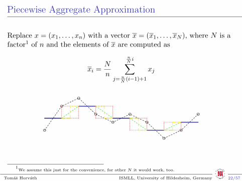
Piecewise Aggregate Approximation

Replace x = (x1, . . . , xn) with a vector x = (x1, . . . , xN ), where N is afactor1 of n and the elements of x are computed as

xi =N

n

nNi∑

j= nN(i−1)+1

xj

1We assume this just for the convenience, for other N it would work, too.


Symbolic Aggregate Approximation

Approach

1 normalize time series x to N (0, 1)

2 provide PAA on the normalized x

3 discretize resulting averages of PAA into discrete symbols


SAX: Breakpoints

An important thing is to discretize1 in a way that symbols of thealphabet α = {α1, . . . , αk} are produced with equiprobability.

• It was empirically discovered on more than 50 datasets thatnormalized subsequences are normally distributed.

Breakpoints are defined as β = {β1, . . . , βk−1}, with βi < βi + 1 forall i, 1 ≤ i < k − 1, such that2

∀i ∈ {0, . . . , k − 1}βi+1∫βi

1√2πe−

x2

2 dx =1

k

where β0 = −∞, βk =∞.

Breakpoints can be found by looking up in a statistical table.1For more details about mapping the averages to symbols, please, see the references.

2The area under the N (1, 0) Gaussian function from βi to βi+1 is equal to 1

k.


Breakpoints: Example

k 3 4 5 6 7β1 -0.43 -0.67 -0.84 -0.97 -1.07β2 0.43 0 -0.25 -0.43 -0.57β3 – 0.67 0.25 0 -0.18β4 – – 0.84 0.43 0.18β5 – – – 0.97 0.57β6 – – – – 1.07

SAX=⇒

(2, 5, 6, 4, 3, 4, 3, 1, 2, 4) (CACDC)


Critical points

There are cases, especially in financial time series, when data containsome critical points.

• difficult to identify them by PAA, and thus SAX, too.


Extended SAX

For each segment Sk we also store the symbols smin and smax for theminimal and maximal values of the segment in addition to the symbolsmean representing the mean value of the segment.

< s1, s2, s3 >=

< smax, smean, smin > if pmax < pmean < pmin< smin, smean, smax > if pmin < pmean < pmax< smin, smax, smean > if pmin < pmax < pmean< smax, smin, smean > if pmax < pmin < pmean< smean, smax, smin > if pmean < pmax < pmin< smean, smin, smax > if pmean < pmin < pmax

where pmin, pmean and pmax are the positions for the minimal, meanand maximal values in the segment, respectively.


Extended SAX: Example

SAX: “BC”Extended SAX: “CBAECC”


Static distance measures

For two time series with the same length.

• Euclidean distance

dEU (x1, x2) =

√√√√ l∑j=1

(x1j − x2j)2

• Euclidean distance on the representations of time series

dREU (x1, x2) =

√√√√ l∑j=1

(R(x1)j −R(x2)j)2

where R : T → C can be – among other possibilities – defined as

R(x) = DFT (x),R(x) = DHWT (x) orR(x) = PAA(x)


Dynamic distance measures

Static distance measures compare the values at the same positions,while dynamic distance measures rather compute the so-called “costof transformation“ of one time series to another.


Warping path

We have

• sequences x = (x1, . . . , xn) and y = (y1, . . . , ym)

• local distance measure c defined as c : R× R→ R≥0• cost matrix C ∈ Rn×m defined by C(i, j) = c(xi, yj)

The goal is to find an alignment between x and y having minimaloverall cost1.

An (n,m)-warping path is a sequence p = (p1, . . . , pL) withpl = (il, jl) for 1 ≤ il ≤ n, 1 ≤ jl ≤ m and 1 ≤ l ≤ L satisfying thefollowing conditions:

• Boundary condition: p1 = (1, 1) and pL = (n,m)

• Monotonicity condition: n1 ≤ ... ≤ nL and m1 ≤ ... ≤ mL

• Step size condition: pl+1 − pl ∈ {(1, 0), (0, 1), (1, 1)} for 1 ≤ l < L

1Running along a ”valley“ of low costs within C.


The DTW distance

An (n,m)-warping path defines an alignment between the two timeseries x and y by assigning the element xil of x to the element yjl of y.

The total cost cp(x, y) of p is defined as

cp(x, y) =

L∑l=1

c(xil , yjl)

The DTW distance is defined as

DTW (x, y) = min { cp(x, y) | p is an (n,m)-warping path }


Some properties of DTW

Let x = (1, 2, 3), y = (1, 2, 2, 3) and z = (1, 3, 3) be time series andc(a, b) = I(a 6= b)

• c is a metric1

DTW does not satisfy triangle inequality

• DTW (x, y) = 0, DTW (x, z) = 1, DTW (z, y) = 2

DTW is generally not unique

• p1 = ( (1, 1), (2, 2), (3, 2), (4, 3) ), cp1(x, y) = 2

• p2 = ( (1, 1), (2, 1), (3, 2), (4, 3) ), cp2(x, y) = 2

• p3 = ( (1, 1), (2, 2), (3, 3), (4, 3) ), cp3(x, y) = 2

1i.e. satisfies non-negativity (c(a, b) ≥ 0), identity (c(a, b) = 0 iff a = b), symmetry (c(a, b) = c(b, a))

and triangular inequality (c(a, d) ≤ c(a, b) + c(b, d)) conditions


Accumulated cost matrix

One way to determine DTW (x, y) would be to try all the possiblewarping paths between x and y.

• computationally not feasible – exponential complexity

An accumulated cost matrix D ∈ Rn×m is defined as

D(i, j) = DTW (x1:i, y1:j)

where i ∈ {1, . . . , n}, j ∈ {1, . . . ,m} and x1:i, y1:j are prefix sequences(x1, . . . , xi) and (y1, . . . , yj), respectively.

Obviously, the following holds

DTW (x, y) = D(n,m)


Efficient computation of D (1)

Theorem: D satisfies the following identities:

D(i, 1) =

i∑k=1

c(xk, y1) for 1 ≤ i ≤ n

D(1, j) =

j∑k=1

c(x1, yk) for 1 ≤ j ≤ m

and

D(i, j) = min{D(i− 1, j − 1), D(i− 1, j), D(i, j − 1)}+ c(xi, yj)

for 1 < i ≤ n and 1 < j ≤ m.

In particular, DTW (x, y) = D(n, n) can be computed in O(nm).



Proof: If i ∈ {1, . . . , n} and j = 1 then there is only one possiblewarping path between x1:j and y1:1 with a total cost

∑ik=1 c(xk, y1).

Thus, the formula for D(i, 1) is proved as can be analogously provedthe formula for D(1, j), too.

For i, j > 1 let p = (p1, . . . , pL) be an optimal warping path for x1:i andy1:j .From the boundary condition we have pL = (i, j).From the step size condition we have(a, b) ∈ {(i− 1, j − 1), (i− 1, j), (i, j − 1)} for (a, b) = pL−1.Since p is an optimal path for x1:i and y1:j , so is (p1, . . . , pL−1) for x1:aand y1:b. Because D(i, j) = c(q1,...,qL−1)(x1:a, y1:b) + c(xi, yj), theformula for D(i, j) holds.



Initialization

• D(i, 0) =∞ for 1 ≤ i ≤ n• D(0, j) =∞ for 1 ≤ j ≤ m• D(0, 0) = 0

The matrix D can be computed in a column-wise or a row-wisefashion. The computation of the whole matrix is needed for getting anoptimal warping path.


DTW: Example


Avoiding the computation of the entire D

Restricting the size of the warping window to a pre-defined constant θ

• D(i, j) is calculated only for those cells (i, j) for which |i− j| ≤ θ.• restricting the computation “near” to the main diagonal of D.

• constant window size or Itakura Parallelogram


Time-Series Classification

Conventional classification techniques can be used depending on thetime-series representation and the distance measure used

• Instance-based• employing DTW• empirically showed that using nearest-neighbor classifiers with

DTW distance measure performs very well

• Memory-based techniques• TS should be represented as vectors of the same length

• PAA, SAX, first k koefficients of DFT, HWT, . . .• Other features derived from TS, as e.g. average, min, max, motifs,

wildcards, . . . .


Motifs & Wildcards

Motifs – characteristical, recurrent patterns in time series

Wildcards – constructed from the taxonomy of symbols


Forecasting: Example

# of new customers of a small company

YearMonth

Jan Feb Mar Apr May Jun Jul Aug Sep Oct Nov Dec1 4 6 9 12 8 14 16 15 14 11 12 102 11 13 14 17 19 19 21 20 18 17 15 14

How many customers will join the company in March of the Year 3?


Seasonality, Trend & Noise in TS

The main components time series usually consist of are

• Noise• a “random” fluctuation in time series• we cannot explain, thus, it is hard to predict

• Trend• the number of new customers are growing from Year to Year• possible to detect

• Seasonality• more new customers are joining the company in summer• possible to detect

In case of no trend and seasonality, a simple smoothing (e.g. averaging)could be eligible to forecast, while if a trend is present, some regressiontechniques could be used.


Forecasting: A straight approach (1)

Getting the seasonality and the trend

• Compute the Seasonal Indices

1 compute the ratios of the value of each month to the average valueof the corresponding Year1

2 compute the average ratios2 for given months.

# of new customers of a small company

YearMonth

Jan Feb Mar Apr May Jun Jul Aug Sep Oct Nov Dec1 4 6 9 12 8 14 16 15 14 11 12 102 11 13 14 17 19 19 21 20 18 17 15 14SI 0.52 0.67 0.84 1.06 0.94 1.22 1.37 1.29 1.19 1.02 1.00 0.88

• Compute the trend using regression from total Yearly sales

Year (Y) Total sales (T)1 1312 198

T = 67 · Y + 64

1Average values are 10.92 and 16.5 for Years 1 and 2, respectively.

2The SI for March is (9/10.92 + 14/16.5)/2 = 0.84.


Forecasting: A straight approach (2)

Forecasting for March of the Year 3

1 Predict the total number of new customers for the Year 3

T = 67 · 3 + 64 = 265

2 compute average monthly value for the Year 3, i.e. 265/12 = 22.083 multiply the average monthly value for the Year 3 with the

seasonal index for March to get the forecast, i.e.22.08 · 0.84 = 18.55


Smoothing

In our previous example, we computed the trend and the seasonality,however, didn’t count with the noise.

• smoothing the time series would be beneficiary for “getting rid” ofthe noise

The most simplest smoothing techniques are

• Moving Average

xt =xt + xt−1 + · · ·+ xt−n+1

N

• Centered Moving Average

xt =xt−k + xt−k+1 · · ·+ xt + xt+1 + · · ·+ xt+k

2k + 1


Moving Average: Example


Single Exponential Smoothing

If there is no significant trend nor seasonality in a time series, wecan use its average to estimate future values.

• A simple average weights each value equally, however the valueswhich are far from the smoothed one should have less weights.

Single Exponential Smoothing (SES) weight past observations withexponentially decreasing weights, i.e.

xt = αxt−1 + (1− α)xt−1

where 0 < α ≤ 1, t ≥ 3 and x2 = x1.

Forecasting with SES is then made in the following way

xt+1 = αxt + (1− α)xt = xt + α(xt − xt)


SES: Bootstrapping & Example

When there are no actual observations for forecasting, we use the lastdata point xn, i.e.

xn+k = αxn + (1− α)xn+k−1, k ≥ 1

We choose α, which results in a smallest error.


Double Exponential Smoothing

If a trend is present in the data, SES doesn’t work well. In this casewe need to

• adjust the smoothed values to the trend of the previous values, and

• update, and also, smooth the trend simultaneously

Double Exponential Smoothing (DES) is computed as:

xt = αxt + (1− α)(xt−1 + rt−1), 0 ≤ α ≤ 1

rt = γ(xt − xt−1) + (1− γ)rt−1, 0 ≤ γ ≤ 1

where t ≥ 2 and r refers to a smoothed trend, initialized e.g. as

r1 = x2 − x1 or r1 =xn − x1n− 1

The m-periods-ahead forecast is computed as

xt+m = xt +m · rt


DES: Example

The results of DES for α = 0.9 and different values for γ

We choose α, γ, which results in a smallest error when comparing theoriginal series to one-step-ahead forecast

• Since we use the current value of the time series to compute thesmoothed value


The Holt-Winters Method

The Holt-Winters method (HWM) is computed as:

xt = αxtst−L

+ (1− α)(xt−1 + rt−1), 0 ≤ α ≤ 1

rt = γ(xt − xt−1) + (1− γ)rt−1, 0 ≤ γ ≤ 1

st = βxtxt

+ (1− β)st−L, 0 ≤ β ≤ 1

where t > L, L is the length of a season and s refers to a sequence ofsmoothed seasonal indices, initialized1 e.g. as was showed before.

The trend factor can be initialized2 as

rL =1

L

(xL+1 − x1

L+ · · ·+ xL+L − xL

L

)The m-periods-ahead forecast is computed as

xt+m = (xt +m · rt) · st−L+m1At least one complete season is needed to initialize seasonal indices.

2The use of two complete seasons is advisable to initialize the trend factor.


HWM: Example (1)

Results of a simple implementation for different extremes of (α, γ, β)


HWM: Example (2)

Different initialization techniques, also the normalization of seasonalfactors should be considered when forecasting1

1See (Chatfield & Yar, 1988) in the references, for more details.


Summary

Representation of time series

• Discrete Fourier & Haar transforms• While FT captures the “global” periodic behavior, HT captures

both “local and global” character of time series.

• PLA, PAA and SAX• One can combine the bottom-up with and Sliding Windows

approaches for more efficient computation.• Despite its simplicity, PAA is often enough to use. Moreover, its

runtime is linear.• SAX representation enables us to use “string-processing” techniques

such as subsequence matching, etc.

• Also other techniques, for example, Singular Value Decomposition.


Summary

Distance measures

• Static distance measures• When time-series are of the same lengths• Use different features derived from time series to represent them in

a common space

• Dynamic Time Warping• Works well even if time series are of different length• Computes a “cost of transformation” between two time series• Plays an important role in classification of time-series with k-NN

• Motifs and Wildcards

• Different variations and speed-ups of DTW

• Forecasting• Seasonality, Trend and Noise• Simple, Double and the Holt-Winters smoothing• Good and well-suited initialization is important• Other forecasting methods, as for example ARIMA


References

• Image Processing lecture slides at UHihttp://www.ismll.uni-hildesheim.de/lehre/ip-08w/script/index en.html

• E. Keogh, S. Chu, D. Hart and M. Pazzani (2001). An Online Algorithm for Segmenting TimeSeries. In Proceedings of IEEE International Conference on Data Mining, 289-296.

• J. Lin, E. Keogh, S. Lonardi and B. Chiu (2003). A Symbolic Representation of Time Series, withImplications for Streaming Algorithms. In proceedings of the 8th ACM SIGMOD Workshop onResearch Issues in Data Mining and Knowledge Discovery. San Diego, CA.

• B. Lkhagva, Y. Suzuki, K. Kawagoe. Extended SAX: Extension of Symbolic AggregateApproximation for Financial Time Series Data Representation.

• Meinard Muller. Information Retrieval for Music and Motion, Springer-Verlag, ISBN978-3-540-74047-6, 2007, 318 p.

• Krisztian Buza. Fusion Methods for Time-Series Classification. PhD thesis, University ofHildesheim, 2011.

• Engineering Statistics Handbook (NIST Sematech)http://itl.nist.gov/div898/handbook/

• Ch. Chatfield and M. Yar (1988). Holt-Winters forecasting: some practical issues. TheStatistician, 1988 vol. 37, 129-140.

• Time-Critical Decision Making for Business Administrationhttp://home.ubalt.edu/ntsbarsh/stat-data/forecast.htm


Thanks for Your attention!

Questions?

[email protected]

Documents

Tom a s Horv ath BUSINESS ANALYTICS · s;tare the smoothed values of fin the corresponding spectrum s coe cients c s;trepresent the di erences in values of fin the corresponding spectrum