TOLERANCE USING ASYMMETRIC INLET

ENHANCED COMPRESSOR DISTORTION

TOLERANCE USING ASYMMETRIC INLET

GUIDE VANE STAGGER

by

Andreas Schulmeyer

B.S., University of Illinois, (1987)

SUMMITED IN PARTIAL FULFILLMENT

OF THE REQUIREMENTS FOR THE DEGREE OF

MASTER OF SCIENCE

IN AERONAUTICS AND ASTRONAUTICS

at the

MASSACHUSETTS INSTITUTE OF TECHNOLOGY

August 1989

c Massachusetts Institute of Technology

Signiture of Author ...Department of Aeronautics and Astrondhtics, August, 1989

Certified byProfessor Edward M. Greitzer

Thesis SupervisorDepartment of Aeronautics and Astronautics

Accepted byProfessor Harold Y. Wachman

ntC~,nt Graduate Committee

t 2 9 1989 VITHDRAWNM.I.T.

UORAM LIBRARlfiSAero

.I ~- E-~

Enhanced Compressor Distortion Tolerance'UsingAsymmetric Inlet Guide Vane Stagger

byAndreas Schulmeyer

Submitted to the Department of Aeronautics and Astronauticýson August 28, 1989 in partial fulfillment c:f therequirements for the Degree of Master of Science

in Aeronautics and Astronautics

ABSTRACT

This w6rk is experimental verification of a method ttoincrease axial compressor distortion tollerance. The methoduses a restagger of the inlet guide vanes to achieve thedesired uniform inlet velocity profile. In order to achievethis the vanes are opened in the low total pressure region,increasing mass flow and pressure rise in this section, andclosing the vanes in the high total pressure region toreduce the mass -flow and pressure rise in this section ofthe compressor.

The theoretical calculations showed that a ten degreerestagger of the guide vanes would achieve the desiredresult for a one dynamic head total pressure distortion.This setup was then tested on the MIT low-speed single stagecompressor. The test data showed the improved performance ofthe restaggered compressor. The non--uniformity in the inletvelocity is reduced by 50%, while presssure rise at stall is5.3% higher than without the restagger and the stall flowcoefficient is 2.7% higher.

Thesis Supervisor: Edward M. Greitzer

Title: Professor of Aer'onaut-i cs and Astronautics

ACKNOWLEDGEMENTS

I would like to offer my thanks to my advisor,

Professor E.M. Greitzer, for his support in solving many of

the unexpected mysteries that the experimental results

provided.

Thanks to Gwo-Tung Chen for his theoretical work which

set the basis for this experimental investigation as well as

the patient introduction he gave me to the methods of this

scheme.

I also appreciate all the help provided by Viktor

Dubrowski, Roy Andrew, Jim Nash and Jerry Guenette with the

experimental setup.

I would also like to thank all my friends at the GTL

and at Ashdown for making life at MIT so much more

enjoyable.

Most of all I would like to thank my parents, Gerhard

and Helga Schulmeyer, for all their love and encouragement

that have made it possible for me to be where I am.

This work was supported by the Air Force Office of

Scientific Research under contract AFOSR -87- 0398E.

TABLE OF CONTENTS

Abstract 2

Acknowledgements 3

List of Tables 5

List of Figures 6

List of Symbols 9

Chapter 1 Introduction 10

Chapter 2 Theoretical Model and Calculations 13

2.1) Introduction 132.2) Compressor Characteristic Calculations 132.3) Distortion Theory Summary 162.4) Restaggering Scheme Calculations 18

Chapter 3 Experimental Setup 21

3.1) Introduction 213.2) Blading Modifications 223.3) Blade Row Spacing 233.4) Distortion Screen Design and Placement 233.5) Instrumentation Layout 243.6) Experimental Procedure and Data Aquisition 25

Chapter 4 Experimental Results 27

4.1) Compressor Characteristics 274.2) Restaggering Scheme Calculations 294.3) Baseline Compressor Behaviour 304.4) Restaggered Compressor Behaviour 314.5) Limitations 33

Chapter 5 Conclusions and Recomendations for Future Work 35

5.1) Conclusions 355.2) Recomendations for Future Work 35

References 37

Appendix Actuator Disc Modeling 38

Tables 42

Figures 44

LIST OF TABLES

Tab I e

2.1 Compressor Geometry

3.1 Distortion Screen Total Pressure Loss Coefficient

42

43

LIST OF FIGURES

Figure

1.1 Typical Allocation of Required Surge Margin 44

1.2 Parallel Compressor Description of Response to 45Circumferential Distortion

1.3 Effect of Non-Axisymmetric Vane Stagger on 46Compressor Response to Total Pressure Distortion

2.1 Three Stage Compressor Response to Three 47Restaggering Schemes

2.2 Empirical Curve Relating Loss Coefficient and 48Diffusion Factor

2.3 Multiplying Factor on Loss Coefficient as a Funtion 48of Diffusion Factor

2.4 Deviation 'Adder' Applied to Carter's Rule as a 49Function of Diffusion Factor

2.5 Calculated and Experimental Data for 4 Low Speed 50Three-Stage Compressors

2.6 Compressor Speedline for Control Modelling 51

2.7 Experimental Speedline 52

2.8 Compressor Speedline with a 10 Degree Opening 53and Closing of IGVs and Stators

2.9 Inlet Total Pressure Distortion Profile 54

2.10 Compressor Response to a 1.0 Dynamic Head 55Distortion with a 5,10, 15 Degree Restagger ofthe IGVs and Stators Near Stall

2.11 Compressor Response to a 1.0 Dynamic Head 55Distortion with a 5,10,15 Degree Restagger ofthe IGVs and Stators at Design Flow

2.12 Compressor Response to a 1.0( Dynamic Head 56Distortion with a 8,12,16 Degree GraduatedRestagger of the IGVs and Stators Near Stall

2.13 Compressor Response to a 1.0 Dynamic Head 56Distortion with a 8,12,16 Degree GraduatedRestagger of the IGVs and Stators at Design Flow

2.14 Compressor Response to a 1.0 Dynamic Head 57Distortion with a Shifted Graduated Restaggerof the IGVs and Stators Near Stall

2.15 Compressor Response to a 1.0 Dynamic Head 57Distortion with a Shifted Graduated Restaggerof the IGVs and Stators at Design

2.16 Compressor Response to a 1.0 Dynamic Head 58Distortion with a 20,30,40 Degree IGV RestaggerNear Stall

2.17 Compressor Response to a 1.0 Dynamic Head 58Distortion with a 11,22,33 Degree IGV Restaggerat Design

3.1 Axial Velocity Perturbation Introduced by a 5910 Degree IGV Restagger vs. Blade Row Spacing

3.2 Circumferential Inlet Total Pressure Profile 60with Inlet Distortion

3.3 Pressure Instrumentation Layout 61

3.4 Velocity Measured by Pitot Tube vs. Velocity 62Measured by Total Pressure Kiel Probes andStatic Pressure Taps

3.5 Scannivalve 1 Pressure Transducer Calibration 63Curve

3.6 Scannivalve 2 Pressure Transducer Calibration 63Curve

3.7 Flow Coefficient from Averaged Pressure Readings 64vs Coefficient from Averaged Local Flow

4.1 Compressor Speedline for 7.5, -7.5 and 22.5 65Degree IGV Stagger

4.2 Compressor Speedline for 0.0 and 27.5 Degree 65IGV Stagger

4.3 Compressor Speedline for 7.5, 15.0 and 22.5 66Degree IGV Stagger

4.4 Inlet Static Pressure Profile at Design Flow 67

4.5 Inlet Velocity Profile Near Stall 67

4.6 Exit Static Pressure Profile at Design Flow 68

4.7 Compressor Speedline Curvefit for Restagger 69Calculation

4.8 Change in Pressure Rise due to Change in IGV 70Stagger Angle vs Flow Coefficient

4.9 Compressor Characteristic Slope vs Flow 70Coefficient

4.10 Calculated Compressor Response to a 1.0 71Dynamic Head Distortion with 5,10,15 DegreeIGV Restagger Near Stall

4.11 Calculated Compressor Response tp a 1.0 72Dynamic Head Distortion with 5,10,15 DegreeIGV Restagger at Design Flow

4.12 Calculated Compressor Response to a 1.0 72Dynamic Head Distortion with 5,10,15 DegreeSquare Wave Restagger at Design Flow

4.13 Compressor Speedline for 15 Degree IGV Stagger 73with and without Inlet Total Pressure Distortion

4.14 Inlet Velocity Profile for Baseline Compressor 74with Inlet Total Pressure Distortion Near Stall

4.15 Inlet Velocity Proflie for Baseline Compressor 74with Inlet Total Pressure Distortion at Design Flow

4.16 Velocity Non-Uniformities for Baseline Compressor '75with 1.0 Dynamic Head Inlet Total Pressure Distortion

4.17 Magnitude of First, Second and Third Fourier 75Coefficients of Velocity Non-Uniformity f'orBaseline Compressor with Inlet Distortion

4.18 Magnitude of Axial Velocity Perturbation for an 76Isolated Rotor with a 10% Inlet VelocityNon-Uniformity

4.19 Restaggered and Baseline Compressor Speedline 77with Inlet Total Pressure Distortion

4.20 Inlet Static Pressure Profile for Baseline and 78Restaggered Compressor Near Stall

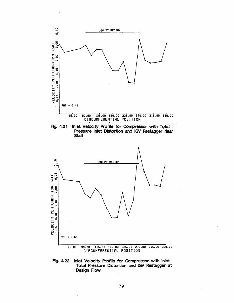
4.21 Inlet Velocity Profile for Compressor with Inlet 79Total Pressure Distortion Near Stall

4.22 Inlet Velocity Profile for Compressor with Inlet 79Total Pressure Distortion at Design Flow

4.23 Velocity Non-Uniformities for Restaggered 80Compressor with 1.0 Dynamic Head Inlet TotalPressure Distortion

4.24 Magnitude of First, Second and Third Fourier 80Coefficients of Velocity Non-Uniformity forBaseline and Restaggered Compressor

4.25 Phase of First, Second and Third Fourier 81Coefficients of Velocity Non-Uniformity forBaseline and REstaggered Compressor

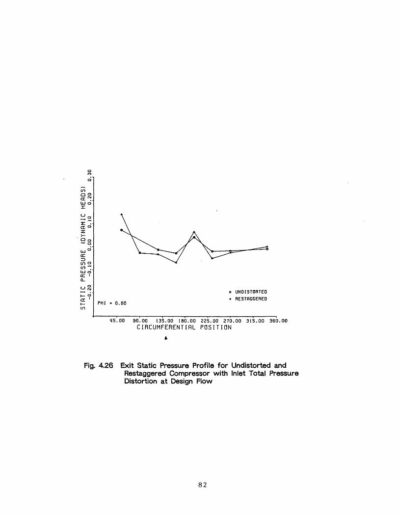
4.26 Exit Static Pressure Profile for Comressor with 82Inlet Total Pressure Distortionand IGV Restaggerat Design Flow

List of Symbols

C Velocity

Ci Blade chord

cp Pressure rise coefficient across blade row

P Non-dimensional pressure

R Mean radius

r Blade stagger angle

a Absolute flow angle

7 Blade stagger angle

Flow coefficient

P Density

0 Circumferential angle

P Compressor pressure rise

Subscipts

e Exit

in Inlet

t Total

x Axial

y Circumferential

Chapter 1 Introduction

Inlet distortion tolerance is an important factor

affecting the stall margin in modern axial compressors. Up

to one half of the design stall margin (Figure 1.1) may be

allocated to account for the effect of inlet distortion [13.

This margin allows for the non-uniformities in the inlet

flow due to such phenomena as crosswind, high angle of

attack induced inlet seperation or shock-boundary layer

interaction in supersonic inlets. In addition to decreases

in pressure rise and efficiency of the compressor, possible

effects of inlet distortion are rotating stall, combustion

flame out or engine overheating.

For these reasons the effect of inlet distortion on

axial compressors has received much attention in the past

years. Methods have been developed to predict performance

E2,3,43 and stability E5,63 of a compressor operating with

an inlet distortion. The standard methods to reduce engine

succeptability to distortion are to increase the tolerance

to non-uniformities by modifying the engine inlets, or to

lower the operating point to increase the stall margin.

With the capabilities of new electronic controls other

methods to increase distortion tolerance have become

available. The theoretical capability to control the stagger

setting of each individual inlet guide vane (IGV) or stator

blade [73 allows the compressor to be divided into two or

more 'parallel compressors', with an asymmetric restaggering

patern chosen to match the inlet distortion E83. By opening

the vanes in the low total pressure region the -flow

coefficient is increased and the operating point moves away

from stall. In the high total pressure region the vanes are

closed and the flow coefficient is reduced, however, because

this region is operating far from stall the reduction in

flow coefficient does not pose a problem.

The behaviour of a compressor restaggered in this

manner can be shown qualitatively in the response of a

parallel compressor to a inlet total pressure distortion.

The low total pressure zone and the high total pressure zone

operating points are determined by the magnitude of the

inlet distortion and the slope of the compressor

characteristic (Figure 1.2). This leads to a different flow

coefficient in the two regions, with the low pressure zone

operating closer to stall. A non-axisymmetric vane stagger

reduces this velocity non-uniformity by shifting the low

total pressure region speedline to the right and the high

total pressure region speedline to the left (Figure 1.3).

The result of the restaggering is a more uniform flow

coefficient around the compressor circumference and an

increase in stall margin gained by moving the low total

pressure operating point further from stall.

A further benefit of using this method is that the mass

averaged pressure rise is not reduced as much as when

closing all vanes uniformly. A second benefit in terms of

overall engine performance is that the compressor can

deliver a uniform flow to the combustor thus reducing the

I ikelyhoo cd of developing hot spots that cat damage the

turbi ne3.

Th e ob jcect of this thesis is to experimenta I ly

demonstrate this type of" scheme for impjroving inlet

distortion toleraince of arn existi-ng ccompressc-r. The test

vehicle is the single stage compressor at the MIT Gas

Turbine ...aboratory. The results of t f the exper iment are

described in this thesis.

Chapter 2 Theoretical Model and Calculations

2.1) Introduction

The theoretical calculations performed as part of the

distortion control are the application to a specific single

stage compressor of the method described by Chen et al. for

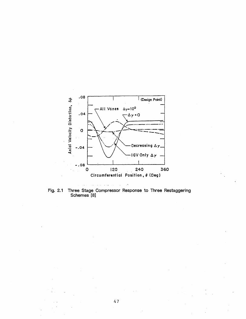
axial compressors. The work in E83 consisted of calculating

the characteristics for a three stage compressor and

implementing the control sceme on this compressor. The

procedure used to calculate the off-design performance was

shown to lead to speedlines in agreement with experimental

data. The computations also indicated that the distortion

control is capable of reducing the velocity defect due to a

distortion of greater than two dynamic heads by a factor of

two (Figure 2.1).

This chapter deals with the prediction of the

compressor characteristic, a summary of the distortion

computations and the application of the computations to the

single stage compressor.

2.2) Compressor Characteristic Calculation

The program used to calculate the off-design behaviour

of the compressor was written by Chen E86 based on a model

proposed by Raw and Weir [93. Losses are calculated -for the

blade rows by using a loss parameter based on the diffusion

factor (Figure 2.2), with a multiplication factor dependent

on blade Reynolds number (Figure 2.3) applied. Carter's rule

for deviation is modified by an "adder' which is a function

of the diffusion factor of the blade rows (Figure 2.4).

The major assumptions of the analysis are:

- high hub to tip ratio, so mean line velocity

triangles are used

- low Mach number so compressibility is neglected

- blades are represented by circular arcs

The last assumption leads to deviations in reasonable

agreement with experimental data, as the turning is

overestimated by neglecting real -fluid effect and by

neglecting thickness turning is underestimated. These two

effects are of comparable magnitude [10) for a solidity of

order one, the solidity of the rotor and stator rows in the

experimental compressor.

The required inputs to the program are the rotor and

stator camber and stagger angles and the IGV leaving angle.

The compressor characteristic and the flow angles are then

calculated for any desired range of flow coefficients.

For the three stage compressors used in previous

calculations the agreement between the calculated arnd

experimentally obtained speedlines is close enough for the

control calculations that followed (Figure 2.5).

The results for the single stage compressor, however,

showed a characteristic that continues to rise as the flow

coefficient deceases (Figure 2.6). From these calculations

it was not possible to predict the compressor stall point

(or the pressure rise at stall) with any precision. The

model does not perform satisfactorally for the single stage

compressor possibly because the correlations used to predict

losses are optimized for multi-stage compressors. The

factors are thus optimized for multi-stage compressors.

Even though the program calculated speedlines that are

not comparable to the experimental speedlines, that were

later obtained (Figure 2.7), the calculated curves were used

to determine the amount and location of restaggering

required to reduce the magnitude of the velocity distortion.

The restagger ing calculations are possible with the

calculated speedlines as the method uses the relative

changes in pressure rise due to a change in stagger and the

slope of "the characteristic as the relevant parameters. For

the actual amount o-f restaggering required the experimental

speedlines could then be used to repeat the calculations. To

find the optimum restaggering method the calculated

speedlines were then used with the point of inflection, the

point where the calculated speedline is the 'flattest', as

the calculated 'stall' point.

The program was then used to calculate various

speedlines. The final compressor geometry can be found in

table 2.1 and the calculated characteristic in figure 2.6.

The stacking of the speedlines required for this control

scheme is shown in figure 2.8 where the nominal speedline is

bracketed by the speedlines with a 10 degree opening and

closing of the IGVs and stators. From this family of curves

the parameters necessary for the restaggering calculations,

15

•a-o•• and a''/a , can be obtained.

2.3) Distortion Theory Summary

This section is a summar'y of the theory developed by

Chen fo:'r a compressor operating with a steady inlet

distortion. The pressure rise across a blade row is given by

an axisymmetric part and an asymmetric component due to the

fluid acceleration within the blade row. The fluid mechanics

for compressor response to total pressure inlet distortion

is described in [53.

With a linearized upstream and downstream flowfield the

compressor performance is given by

where

SCi

cos r4

is the parameter associated with fluid acceleration

within the blade rows. C, r, R are the chord, stagger and

mean radius, respectively, of the rotor.

For a small disturbance the downstream pressure field

satisfies

VP2 P =O (2.2)

and the boundary condition at the compressor exit plane is

aPc ac, + cac(P a• "=O a• =oy

16

results obtained

Eq. (2.2) and (2.3) are

6=- i aq a6o+ - a o--+ r ST-a

and

= 0' sec' aa6aI

(2.5)

Expanding all variables in Fourier series

+oo

6i =C a, einae-lniz

+oo

65i= z d enin#n -oc69 = n b eini

+-00

Sy = E dn iniL= -0O

and subsituting Eq. (2.6),(2.8) and (2.9) into Eq. (2.5) we

have

znan= - sec'IIn bn + dn)

89n

Comb i n i ng (2.4),(2.7),(2.8) ,(2.9) and (2.10)

S in se ) d en- i sec c a1'

-nA +- seC in • c•p- Tc-o

a6 ,PaZ 1,=0

(2.6)

(2.7)

(2.8)

(2.9)

(2.10)

bn - (2.11)

The linearized from perturbing

The stagger distribution that eliminates the velocity

distortion, i.e.

(2.12)6 =0, b =O

is given by

d, -17-- a (2.13), 02 _eC2 C1 '3.7en a , seco a+

2.4) Restaggering Scheme Calculations

The program that calculates the characteristics for the

compressor also provides the two variables a.i/ay and

YT/D~ that determine the behaviour of the compressor with an

inlet distortion and the implemented restagger. These two

derivatives are needed to t•d calculate the velocity profile

of the compressor with an inlet total pressure distortion

and various stagger profiles. The goal is to find a stagger

profile to minimize the velocity non-uniformity at the face

of the compressor. For the calculations the inlet total

pressure distortion is a sine shaped defect over 180 degrees

of the annulus with a magnitude of one dynamic head (Figure

2.9).

Based on the work done by Chen two schemes were used in

the first set of calculations. The first is a restagger of

both IGVs and stators identical amounts in phase with the

total pressure distortion. The results can be seen in the

resulting axial velocity distribution for the compressor

operating near stall (Figure 2.10) and at design flow

(Figure 2.11). For both of these the velocity defect due to

the distortion are of the same shape and magnitude, as in

both cases the slope of the characteristic and al~Y are

almost identical. The capability to correct the velocity

defect at both flow coefficients is also of the same order

resulting in almost identical behavior for both cases. The

magnitude of the velocity distortion is reduced by almost a

factor of two for both flows although there is still a

defect remaining. It is not possible to reduce the velocity

non-uniformity any further with this scheme, as a larger

restaggering leads to an overcorrection in parts of the

circumference, which can be seen in the 15 degree restagger

of the blade rows.

This led to the attempt to reduce the velocity

distortion by restaggering the stators and IGVs differing

amounts, still in phase with the pressure distortion. A

sampling of the resultant velocity profiles, of the case

where the stator restagger is 3/4th of the IGV restagger,

can be seen in *figures 2.12 and 2.13. Here again it was

possible to reduce the velocity distortion by a factor of

two, but the velocity profile still shows the same behaviour

as the previous calculations.

The next step allowed for a phase shift between the

restaggered regions and the pressure distortion. The model

was extended in this case to allow for the phase shift

between the restaggering in the two blade rows. In this case

the repsonse to a stator restagger is calculated separately

from the response to a IGV restagger. This extension of the

model assumes that the velocity perturbations introduced by

the restagger of the stators does not alter the velocity

perturbation introduced by the IGVs if both are calculated

separately and vice versa. This is possible as the

:Linearization in the model assumes that DI/0 and aayan

remain constant even with the velocity perturbations

introduced by the total pressure distortion, or in this case

by the restagger of the other blade row. The final result is

then obtained by summing the effect of the individual blade

row restaggerings. This method introduces the phase shift as

a new degree of freedom and should thus lead to an improved

velocity profile.

As -figures 2.14 and 2.15 show a reduction of the flow

non-uniformity can be achived in this manner. The magnitude

of the velocity distortion can be reduced by a factor of

four or more. The complexity of this scheme, however,

detracts from its attractiveness so that further schemes

were tested.

The most efficient method to reduce the velocity

distortion was found to require a restaggering of the IGVs

only. This method (Figures 2.16 and 2.17) is capable of

completly removing the velocity distortion, but it is

limited by the amount of restagger of the IGVs possible

without separating the airfoils.

It was decided to use only the restaggering of the IGVs

as the scheme to be implemented. The magnitude of

restaggering is then dependent on the size of the pressure

20

distortion, the change in pressure rise due to the change in

stagger, a/ay , and the maximum restaggering possible

without stalling the blades.

Chapter 3 Experimental Setup

3.1>) Introduction

The GTL single stage compressor was modified for the

experimental investigation. The major changes were the

restaggering of the blade rows, the reduction of stage

spacing, the installation of a distortion screen and added

instrumentation and modification of the data aquisition\

programs. The compressor has a hub to tip ratio of 0.74 and

the design flow rate for the baseline blade setting is 0.59.

A detailed description of the geometry is given in table

2.1.

3.2) Blading Modifications

The IGVs used previously were long chord sheet metal of

high solidity. These were not suitable for the restaggering

required by the distortion ex>periment, as the long chord led

to interference with the outer casing. They also have low

incidence tolerance. The replacement set of IGVs had a

shorter chord thus allowing for the required movement, and,

although they are also sheet metal, somewhat better

incidence tolerance as they are thicker, with a rounded

leading edge.

The new blades were 1/16th inch shorter than the

previous set leading to a clearance around the centerbody of

the compressor. As the centerbody was now supported only at

the front end by six struts three of the 46 IGVs were

22

replaced by bolts to locate the the centerbody and

eliminate vibration.

3.3) Blade Row Spacing

The compressor had been set up with maximum spacing, a

5" gap between the rotor and stator, for the previous

experiment. The effect of spacing was thus investigated

using an actuator disc analysis (see appendix for

derivation), with rotor and stator lumped into one disc and

IGVs as another. The spacing (H), non-dimensionalized by the

compressor radius (R), between the two was varied from the

existing setup down to zero. As the calculations show

(Figure 3.1) the velocity correction introduced with minimal

spacing (H/R = 0.05) is in phase with the IGV stagger

movement from -90 to +90 degrees. For a larger spacing the

velocity correction shifts in the direction of the turning

introduced by the IGVs. This, together with the change in

magnitude, will lead to an incorrect estimate in the

restaggering calculations based on zero spacing. The spacing

between the IGV row and the rotor was therefore reduced to

the minimum possible with the existing compressor

corresponding to H/R = 0.25, although this still left a

significant gap.

The program that calculates the compressor response to

the inlet distortion was not modified to account *for this

spacing between the blade rows due to time constraints on

the program.

23

3.4) Distortion Screen Design and Placement

The screen was designed to give a total pressure

distortion of one dynamic head. It consists of 7 sections

which lead to an approximation of the sine shaped defect

used in the calculations. The total pressure loss

coefficients for each section were determined by rescaling

the screen used by Bruce E113 to obtain a sinusoidal

velocity profile. The circumferrential extension and the

pressure loss coefficient of each section can be *found in

table 3.1.

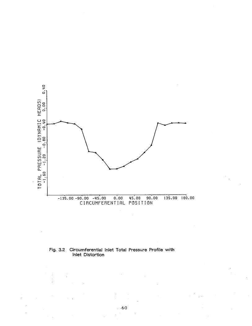
The screen was attached to the forward struts

supporting the centerbody 23 inches ahead of the IGVs, where

it could easily be removed to obtain uniform flow compressor

data. With this large spacing some mixing was ex:pected, the

total pressure profile measured at the IGV plane is shown in

figure 3.2. The overall profile approximates the desired

sinusoidal total pressure defect, except for the reading at

-90 degreesthe interface of the low and high total pressure

regions, which is lower than expected.

3.5) Instrumentation Layout

The instrumentation was set up to give a detailed

circumferential profile in front of the IGV plane and to

measure overall compressor performance. Twenty kiel probes,

for total pressure measurement, and twenty static pressure

taps were installed upstream of the IGVs. Ten more sets were

installed downstream of the stator (Figure 3.3). The close

24

spacing of the kiel probes behind the static pressure taps

led to an increase in the static pressure measured and a

correction factor was calculated by representing the kiel

probe and its wake as a source. The resulting correction

-factor of 1.08 for the axial velocity agrees with the ratio

of the axial velocity measured by a pitot tube compared to

that obtained from the kiel probes and static pressure taps

(Figure 3.4).

Four of the static pressure taps, two at the inlet

plane and two in the downstream set, were not used in the

calculations as they gave incorrect readings whose origion

could not be found.

The calibration curves for the two scannvalves used to

obtain the pressure readings are shown in figures 3.5 and

3.6.

3.6) Experimental Procedure and Data Aquisition

"The basic plan of the experiment was as follows. The

compressor characteristics for IGV settings of +15, 0, -15

relative to the design staggering were first obtained. With

this data lT/ay can be calculated. This determines the

amount of restaggering required to remove the velocity

distortion introduced by the screen. The final speedlines

would then show the difference between the uniformly and

non-ax i symmetricly staggered compressor and show the

improvement in the circumferrential velocity profile.

The individual speedlines are taken starting with the

25

throttle completely open. The throttle is slowly closed to a

new operating point and the procedure repeated until the

stall point is reached. Each of the compressor operating

points is calculated using an average of the inlet total and

exit static pressures to give the total to static pressure

rise. The axial velocity is calculated by averaging the

local velocities obtained from the total and static pressure

probes. This definition of the axial flow coefficient is

also used for the distorted flow where it represents an

average -flow coefficient for the whole compressor.

In distorted flow the overall flow coefficient for the

compressor obtained from averaging the individual velocities

gave a value up to 5% higher than a method using the average

pressure readings (Figure 3.'7). As defined here, therefore,

all axial flow coefficients are those based on the

velocities at the inlet plane.

26

Chapter 4 Experimental Results

4.1) Compressor characteristics

The first sets of data taken were the family of

speedlines needed to calculate the variables aP/o and '/o .

Several IGV stagger settings were used. The inital setup was

an IGV stagger angle of 7.5 degrees (Figure 4.1). As

expected from previous results the agreement with the

calculated speedline was only acceptable near the design

flow coefficient of • = 0.59, so new calculations of the

optimum stagger were performed using the experimentally

obtained speedlines.

Two speedlines were then taken for a change of stagger

of +/- 15 degrees from nominal (Figures 4.1). The

increased stagger of 22.5 degrees led to a decrease in

pressure rise and stall flow coefficient, as predicted by

theory. The speedline with the IGV stagger setting of -7.5

degrees showed an unacceptable drop in pressure rise near

stall, dropping below the pressure rise for the +7.5 degree

stagger. T'he reason for the lower pressure rise is the

separation of the airflow on the IGVs at a high negative

angle of attack. As the l inear model uses only a mean value

of aY/7 a change in sign of T/qY was inappropriate f'or the

range of stagger angles to be used in the control sceme.

Figure 4.2 shows a speedline for a IGV stagger of 0

degrees . Using linear interpolation of the three speedlines

with stagger angles of +7.5, 0 and -7.5 degrees stagger the

27

critical stagger for which 0a~y = 0 is at 3 degrees, which

was taken as the point where the IGVs separated.

To avoid stagger angles for which the sign of

Dii/l~ changes a speedline was taken with an IGV stagger of

27.5 degrees (Figure 4.2). This speedline along with the

speedlines "for +7.5, 15 and 22.5 degress showed the desired

stacking and they were chosen -for the experiment (Figure

4.3).

The nominal setting around which the non-axisymmetric

staggering was then designed was a stagger angle of 15

degrees which allowed for a maximum restagger of up to 10

degrees before separation occured.

The static pressure readings for undistorted flow

(Figure 4.4) showed non-uniformiteis that could not be

accounted for. A correction factor for each probe was

therefore obtained from the raw data. The corrected velocity

profile was then satisfactory near stall (Figure 4.5). The

upstream struts supporting the centerbody, the eccentricity

of the centerbody, the variation of the blabe tip clearence

and other imperfections in the compressor are accounted for

in this correction. The correction in the static pressure

readings accounts for the permanent, i.e. systematic, non-

uniformities in the compressor and the subsequent will show

only changes due to the inlet distortion and the IGV

restagger.

The same correction, to account for blade to blade

variations and other imperfections of the compressor, was

performed on the exit static pressure non-uniformities, but

28

even then it was not possible to reduce the static pressure

non-uniformity at the exit plane to less than .05 dynamic

heads (Figure 4.6).

4.2) Restaggering Scheme Calculations

The parametersaT//ay and DI/ao were determined from the

experimental speedlines. All speedlines were fit with a

third order polynomial (Figure 4.7) and the resulting curve

fits used for a calculation cr'fTl/ayandaTy/aat any operating

point of the nominal speedline. These values (Figure 4.8 and

4.9) are compared with those calculated using the computer

generated speed 1 ines. The experimental values of ~DP/ayand

aYIJ/ were used to find the restaggering required to reduce

the velocity non-uniformity created by the distortion

screen. For the 1.0 dynamic head total pressure distortion a

restagger of 10 degrees was needed (Figures 4.10 and 4.11)

to obtain a sizable reduction in the velocity distortion.

The actual restagger of the IGVs was a square wave with

a +10 degree restagger in the low pressure zone and a -10

degree restagger in the high pressure region. "The square

wave restagger was chosen as a simple sector restaggering

that would show a benefit similar to the more complicated

method of a sinusoidal restagger, where each blade would

have to be restaggered by a different amount. The results of

using a square wave restagger in the calculations can be

seen in figure 4.12. The figure shows that with the 10

degree square wave restaggering it is possible to reduce the

29

velocity non-uniformity by a factor of two.

4.3) Baseline Compressor Behaviour

The compressor was run with the distortion screen

installed and uniform IGV stagger angle to find the baseline

response. The characteristics with and without distortion

are shown in figure 4.13. The pressure rise at stall is 7.9%

lower and the stall flow coefficient decreased from 0.38 to

0.37. The drop in pressure rise is to be expected as a

result of the total pressure inlet distortion.

The velocity profiles for the distorted flow operating

conditions show a more pronounced effect (Figures 4.14 and

4.15). For all flow coefficients the shape of the profiles

are similar and follow that of the total pressure profile.

The large change in flow coefficient at the 0 degree

position can be explained by the presence of one of the

three supporting struts which replaces the IGV at this

location. This large spike appears in the distorted flow, as

the swirl introduced by the inlet distortion leads to a non-

uniform incidence angle on the IGVs around the

circumference. At this larger, non-uniform incidence angle

the strut will therefore have a stronger influence on the

local flow coefficient.

The non-uniformity in the inlet velocity is measured

using three methods. The first method is the rms value, the

second is the sum of the absolute values of the difference

between the average and local flow coefficient and the third

30

is a Fourier analysis of the velocity profile showing the

magnitude of the first three coefficients. Using these

measures of non-uniformity the experimental data shows a

trend opposite to that of the theoretical calculations

(Figure 4.16 and 4.17). The velocity distortion increased

towards lower flow coefficients for the theoretical model,

while the distortion becomes more severe -for higher flow

coefficients in the experiment.

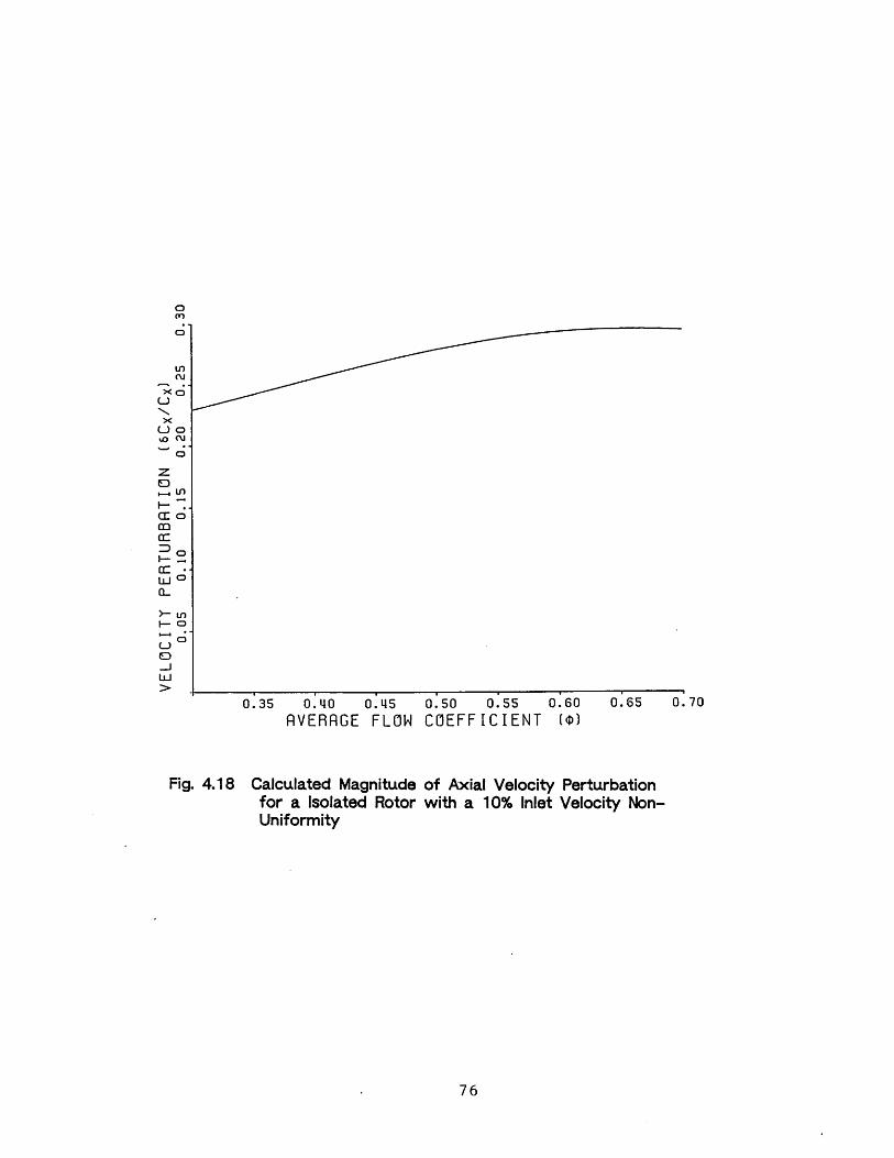
This change in behaviour is thought to be due to the

setup of the compressor. Due to the separation between the

rotor and the stationary blade rows the behaviour of the

compressor has similarities to that of an isolated blade

rotor. Using an actuator disc model of an isolated rotor the

trend observed in the experiment can be predicted. As the

calculations show (Figure 4.18) the velocity non-uniformity,

in this case the maximum amplitude of a sinusoidal velocity

distortion, will increase for higher flow coefficients. The

theory therefore confirms the trend observed in the

experiment. This change in behaviour will modify the

magnitude of the individual distortions, but it does not

effect the control scheme otherwise.

4.4) Restaggered Compressor Behaviour

With the restagger implemented the same sets of data

were then taken to determine the improvement in performance.

The average performance given by the speedline is shown in

Figure 4.19. The stall pressure rise is now 0.38 compared

31

to the baseline 0.36 and the stall flow coefficient moved

from 0.37 to 0.38. The loss in pressure rise is smaller than

in the uncorrected case. The restaggering of the IGVs has

brought the flow coefficient at stall back to the

undistorted ý = 0.38.

The changes in the pressure and velocity profiles show

this improvement of the flow more clearly. The static

pressure is decreased in the region where the vanes are

opened relative to the uniform stagger setup (Figures 4.20).

This leads to an increase of the velocity and thus a

reduction of' the distortion for all flow coefficients. The

non-uniformity of the velocity profiles in the restaggered

setup (Figures 4.21 and 4.22) shows a change from the

baseline case, but a direct comparison is difficult due to

the non-uniformities in the profiles.

A more detailed examination of the restaggered profiles

shows a large increase in velocity in the region between 250

and 290 degrees, as the calculations for the square wave

restagger had predicted. This "spike' is the result of two

side effects of the restagger square wave restagger. The

restaggering provides too much correction here. The static

pressure is reduced even though this section is not in a low

total pressure region, thus leading to an increases in

velocity.

There is also an.effect due to the spacing between the

blade rows. As the actuator disc calculations had shown the

spacing would lead to a correction that would be larger than

the calculated correction for zero spacing, in the direction

32

of the swirl induced by the IGVs. The spike is more extreme

in the experiment due to the abrupt change in stagger at

this location from 5 to 25 degrees. The spike could

therefore be removed if the restagger were implemented

interactively, using a measurement of the local flow

velocity to restagger the IGVs in that region.

The increases in the flow coefficient at 135, 200 and

360 degrees in figures 4.21 and 4.22 are again a result of

the supporting struts.

The comparison of the criteria for distortion magnitude

show a clearer decrease of a factor of two in the velocity

non-uniformities for all flow coefficients (Figure 4.23 and

4.24). For the higher flow coefficients the restagger is not

as effective as for the lower flow coefficients, as it was

desig~ned *for a flow coefficient of ý = 0.45. A comparison

of the phase of the first three harmonics (Figure 4.25)

shows only small changes in the phase of the harmonics.

4.5) Limitations

These results of the response of the compressor to the

distortion and the resulting restaggering show some of the

limits of the basic scheme.

The exit static pressure profile does not agree with

the uniform pressure assumption of the model (Figure 4.26).

This non-uniformity existed with and without the distortion,

and the conclusion is that it is due to the compressor and

33

not due to the restaggering of the IGVs.

The shift of the static pressure profile in direction

of rotor rotation relative to the original total pressure

distortion is ignored in the linear model, which assumes no

spacing between the blade rows. This together with the

sudden change in stagger angle at the interface of the two

regions leads to an interaction of the two sections not

included in the parallel compressor model.

34

Chapter 5 Conclusions

and Recomendations for Future Work

5.1) Conclusions

The results of the implementation of the non-

axisymmetric stagger are encouraging even given the very

non-ideal test conditions. They show that it is possible to

reduce the velocity distortion at the compressor face by a

factor of two with an IGV restagger of 10 degrees. A setup

with closer more typical spacing between the blade rows and

aerodynamically improved IGVs, typical of current axial

compressors, should increase the ability to reduce velocity

distortions and extend the method to even larger inlet total

pressure distortions.

Non-axisymmetric restaggering also reduced the loss in

pressure rise due to the inlet total pressure distortion.

5.2)Recomendations for Future Work

The restaggering required of the IGVs is in the range

possible in current engines. The possibility of

implementing this method opens further questions on overall

engine performance that need to be investigated.

The ability of the scheme to adapt to different inlet

distortions plays a role in its usefulness. If each blade

has to be controlled independently to achieve the reduction

in velocity non-uniformity the improvements will be much

35

smaller, due to the weight and complexity of the actuators,

than if sectors of 60 to 90 degrees can be restaggered by a

single actuator. A future investigation would therefore test

a compressor with inlet total pressure distortion and a

restagger in a certain section with varying phase between

the two, to determine how accurately the restaggering has to

be positioned to obtain a desired decrease in f low non-

uniformity.

Similarly the number of sensors required to determine

the location and magnitude of the distortion will depend on

the level of accuracy needed to show an improvement in

compressor behaviour. Here the work would concentrate on the

number of probes required to locate the inlet distortion.

The implementation of this method in an engine would

then require a quick method, such as a lookup table, that

would specify the amount of restagger required for each

sector according to the extend and magnitude of the

distortion as well as the location of the current operating

point on the speedline. Future work in this area would deal

with the amount of time required between the sensing of an

inlet distortion and the repositioning of the IGVs.

Before this method can be applied to actual compressors

further work will have to be done to compare the relative

gains of implementing this method instead of improvements

gained by an additional compressor stage and the amount of

sensing required to make the restagger ing an efficient

method of improving distortion tollerance.

36

REFERENCE

1) Seymore, J. C., 'Aircraft Perormance Enhancement withActive Compressor Stabilization',MIT Thesis Sept 1988

2) Mazzaway, R. S., 'Multiple Segment Parallel CompressorModel for Circumferential Flow Distortion' , Engineeringfor Power, Vol. 99 No. 2, April 1977

3) Stenning, A. H. , 'Inlet Distortion Effects in AxialCompressors', Journal of Fluid Engineering, Vol. 102,March 1980

4) Reid, C., 'The Response of Axial Flow Compressors toIntake Flow Distortion:', ASME Paper 69-GT.-29, 1969 ASMEGas Turbine Conference

5) Hynes, T. P. and Greitzer, E. M., 'A Method of AssessingEffects of Circumferential Flow Distortion onCompressor Stability', ASME Journal of Gas Turbines andPower,

6) Hynes, T. P., Chue, R., Greitzer, E. M. and Tan, C. S.,'Calculation of Inlet Distortion Induced CompressorFlow Field Instability', AGARD Conference ProceedingsNo. 400, 'Engine Response to Distorted Inflow', March1987

7) Epstein, A. H., '"'Smart' Engine Components: A Micro inEvery Blade?', Aerospace America, Vol. 24, January 1986

8) Chen, G. T., 'Active Control of TurbomachineryInstability - Initial Calculations and Results', MITThesis August 1987

9) Raw, J. A., and Weir, G. C., "'The Prediction of Off-Design Characteristics of Axial and Axial/CentrifugalCompressors', SAE Technical Paper 800628, April 1980

10) Rannie, W.D. ,'The Axial Compressor Stage', Section Fof 'Aerodynamics of Turbines and Compressors',Princeton University Press, 1964

11) Bruce, E. P., 'Design and Evaluation of Screens toProduce Multi-Cycle 20% Amplitude SinusoidalVelocity Profiles', AIAA Paper No. 74-623, AIAA 8thAerodynamic Testing Conference, July 1974

37

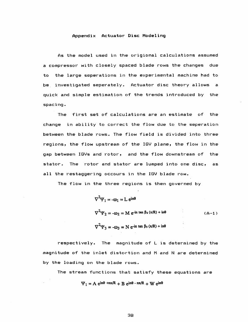
Appendix Actuator Disc Modeling

As the model used in the origional calculations assumed

a compressor with closely spaced blade rows the changes due

to the large seperations in the experimental machine had to

be investigated seperately. Actuator disc theory allows a

quick and simple estimation of the trends introduced by the

spacing.

The first set of calculations are an estimate of the

change in ability to correct the flow due to the seperation

between the blade rows. The flow field is divided into three

regions, the flow upstream of the IGV plane, the flow in the

gap between IGVs and rotor, and the flow downstream of the

stator. The rotor and stator are lumped into one disc, as

all the restaggering occours in the IGV blade row.

The flow in the three regions is then governed by

V1 = -CO =L ein

V22 = -)2 = M e -in tan •1 (x/R) + in (A-)

V2 3 = -03 =N e-in tanP3 (xR) + in

respectively. The magnitude of L is determined by the

magnitude of the inlet distortion and M and N are determined

by the loading on the blade rows.

The stream functions that satisfy these equations are

'1 = A eine +ndR + B e ine - nx/R + W eine

38

'2 = C emne + nx/R + D eine - nx/R + E ein( - x/R tan a2)

Y 3 = F e ino + nx/R + G e in0 - nx/R + H ein( - n/R tan - )

The magni tude of the constants A through H are

determined by the boundary conditions at x = c c and at the

two blade rows x = 0, h.

at x =-- Co is bounded => B = 0

at x = co 'I is bounded => F = 0

At each of the blade rows three boundary conditions

have to be met. Contenuity has to be satisfied, the flow

leaving angle is specified by the blade setting and the

pressure rise is given by the compressor characteristic.

at x = 0

A + W = C + D + E

- itan.a A = C - D - i tan a2E ( -3)

P2 ) = ([2U1 + 2VlV]cp + 2 + V12] a)cR ae ae 2 ae ae ae

at x: =h

C enh/R + D e-n R + E e-inh R tan a 2 = G e-nh/ R +H e-in R tan a3 ( A-4)

in tan a2 (C en + D e- nW + E e- inR tan a2) = - G e- nR + H e- nW tan a3R R

- )= ([2U2 + 2V2 ]c+ [U+ +Vi )R ae ao 2 ae a P ae

the pressure depedency can be removed from the dynamic

equations by substituting the momentum equation

39

U a+ + (A--5)5x Rao pRaO

The velocities are then expressed in the

streamfunctions and the equations linearized by dropping all

second order terms. The resulting 6 x 6 system can then be

evaluated for any desired inlet distortion or IGV blade

distribution.

The other application is the calculation of the effect

of an isolated rotor on a velocity distortion. In this case

the flowfield is divided into an upstream and downstream

region.

V 2i =-

(A-5)

V 2 2 = -02

In this case the pararmeter was the flow coefficient of

the compressor. As a result of this the pressure rise of the

blade row had to be included as a function of the flow

coefficient. The model uses a curve-fit of the nominal

experimental speedline for this, as the calculations are

only intended to show the trend in the magnitude of the

velocity distortion. The change in pressure rise around the

circumference due to the velocity non-uniformity is acounted

for by using the slope of the characteristic at the average

flow coefficient. The flow direction in the downstream

region is now also dependent on the flow coefficient, as the

relative leaving angle is asumed to be constant.

Applying the boundary conditions at x = and at x = 0

and performing the same substitutions as before leads to a 3

£40

x 3 system that can be solved to find the effect of the

rotor.

Rotor Stator

Hub Diameter (rrmn) 444 444 444

Casing Diameter (mn) 597 597 597

Number of Blades 46 44 45

Chord (mrr) 33 38 38

Solidity at Midspan 0.9 1.0 1.0

Aspect Ratio 2.2 1.9 1.9

Camber (deg) 12 25.5 30.0

Midspan Stagger (deg) 15 28.7 45.0

Blade Clearance (rrmn) 1.6 0.8 1.5

Table 2.1Compressor Geometry

IGV

Sector Loss Coefficient(deg) Pt/.5 Rho Cx^2

-90 to -70 1.02

-70 to -30 1.34

-30 to 30 1.72

30 to 70 1.34

70 to 90 1.02

90 to -90 0.32

Table 3.1

Distortion Screen Total PressureLoss Coefficient

43

OPERATING LINE SHIFTOR

SURGE LINE SHIFT

REMAINING

AUGMENTOR SEQUENCING

INLET DISTORTION

ENGINE VARIATION

CONTROL TOLERANCE

REYNOLDS NUMBER

USABLE SURGE MARGIN

MINIMUM SURGE MARGIN

7Fig. 1.1 Typical Allocation of Required Surge Margin [1]

5.5%

5.5%

7.5%

2.5%

1.5%

1.5%

I* 1 I 1 1 IW 10Tal

essure Zone

PTSInlet Distortion

I2High ToPress. Z

I I0.4

I I0.6 0.8

Mass Flow, Cx/U

Fig. 1.2 Parallel Compressor Description of Response toCircumferrential Distortion

45

cliC

0.Ci--

aQ)

0

'1)

a-..

O

0u 0.2

I .

High TotalPress. Zon

Mass Fl

4-

C'30

ow, Cx/U

Fig. 1.3 Effect of Non-Axisymmetric Vane Stagger on CompressorResponse to Total Pressure Distortion

CuJD

a-

L-0U)U)

E0

0)

N IUT Il

Rss. Zone

OpeningVanes

ominal

.08-9-

0

" .04o

0u

.o -. 04

n9

0 120 240 360Circumferential Position, 9 (Deg)

Fig. 2.1 Three Stage Compressor Response to Three RestaggeringSchemes [8]

'06 1

Total pressure.05 - loss parameter

CjaLS Cos 022C1 Co 82 Fully stalled.04 cascade

.03

.02Slgnlficant cascade

.01 --- stall starts here

0U .1 *j *q * a .0 .1 ..3 .4 . .6 .7

DFAC = 1 -V+(S) ACuv, c 2TV -

Fig. 2.2 Empirical Curve Relating Loss Coefficient andDiffusion Factor [91

ni.0n

%.U

3.0

2.0

Multiplyingfactor on@ML

SP-38, fig 1, l I

ix I I1

IN)'" power law

a number 500,0001 1 1 1 1 1 1 1 1

efe rence royno e

II I

1 2 3 4 6 7 8 9 10 11 1 9

R*-blade chord reynolds number x 10-

Fig. 2.3 Multiplying Factor on Loss Coefficient as a Functionof Diffusion Factor [9]

43

51 - -i

LL

Cc

,51

- --

_ -I

0 .I

-- '----

.8 .9

5

I- ~- ~- '-

DFAC = 1 - V + (S)ACu

Fig. 2.4 Deviation 'Adder' Applied to Carter's Rule as aFunction of Diffusion Factor [9]

1.5

1.0

/s

.5

03

0.2 0.4 0.6 0.8 1.0 1.2

Fig. 2.5 Calculated and Experimental Data for 4 Low SpeedThree-Stage Compressors [8]

ROTOR STAGGER = 28.70ROTOR CAMBER = 25.50STATOR STAGGER = 45.00STATOR CAMBER = 30.00

IGV EXIT ANGLE = 15.0

0.35 0.40 0.15 0.50 0.55FLOW COEFFICIENT (0)

0.60 0.65 0.70

Fig. 2.6 Compressor Speedline for Control Modeling

o

o

-- ,

00

I-I -C'

fI,a- C)1-

IGV STAGGER

0 15.0

0.40 0.45 0.50 0.55 0.60FLOW COEFFICIENT - ()

0.65 0.70 0.75

Fig. 2.7 Experimental Speedline

0

,7

.- ,

ROTOR STAGGER - 32.80ROTOR CAMBER - 25.50STATOR STAGGER - 45.00STATOR CAMBER * 26.40

EXIT

CLOSED VANES

OPENED VANES


0.60 0.65 0.70

CC<0

o

0-I

0in -"O~

a-00U)c

0=.-0

Fig. 2.8 Calculated Compressor Speedlines with a 10 DegreeOpening and Closing of IGVs and Stators

53

45.00 90.00 135.00 180.00 225.00 270.00 315.00 360.00

THETR

Fig. 2.9 Inlet Total Pressure Distortion Profile

LuJU)(n

cc

CEI-0I--

STATOR HRAX SWINGSTATOR HAX SWING

45.00 90.00 135.00 180.00 225.00 270.00CIRCUMFERENTIAL POSITION

315.00 360.00

Fig. 2.10 Compressor Response to a 1.0 Dynamic Head Distortionwith a 0,5,10,15 Degree Restagger of the IGVs andStators Near Stall

in 0.0m 5.0

IGV MAX SWINGICV HAX SWING

0.0 STATOR MAX SWING5.0 STATOR MAX SWING

PHI 0.70

IGV PHASE 0.0STATOR PHASE 0.0


315.00 360.00

Fig. 2.11 Compressor Response to a 1.0 Dynamic Head Distortionwith a 0,5,10,15 Degree Restagger of the IGVs andStators at Design Flow

55

0.0 IGV MAX5.0 IGV MAX

SWINGSWING

0.05.0

in

0

0eo

CC0Z ;co

>- 0;I-o

0r,•Oo

0.0r

1-J=_o,i-o

o =,

-JI ocr 0

X•-(I

PHI 0.50

IGV PHASESTATOR PHASE

T0

0

In

0

z00

C;inoco05

IU,

o

x-4U0T0.

-·I

(90.0 IGV HAXM 8.0 IGV HAX

SHINGSWING

0.0 STATOR HRAX SWING6.0 STATOR HRAX SWING

a

oC;

C;tna

z9Qo05--

oC;

CCv-u0.

o

-J.oLLJW

a:•oX•IO,

-4(I IGV PHASE 0.0STATOR PHASE 0.0


315.00 360.00

Fig. 2.12 Compressor Response to a 1.0 Dynamic Head Distotrionwith a 0,8,12,16 Degree Graduated Restagger of theIGVs and Stators Near Stall

SI0.0 IGV HAX SWINGm 8.0 IGV HAX SWING

0.0 STATOR HAX SWING6.0 STATOR HAX SWING

PHI 0.70



315.00 360.00

Fig. 2.13 Compressor Response to a 1.0 Dynamic Head Distotrionwith a 0,8,12,16 Degree Graduated Restagger of the.IGVs and Stators at Design Flow

in

PHI 0.50

0.0 IGV MAX SWING5.0 IGV HAX SWING

0.0 STATOR MAX SWING3.0 STATOR HAX SWING

0

o

<3U,0edWzQo

I-o• Yo

C3CC0.

-JL )

0_ I

0:0XQ:=


Fig. 2.14 Compressor Response to a 1.0 Dynamicwith a Shifted Graduated Restagger ofStators Near Stall

i--ei--

0

I-

>-

-JU

-.J

a:

6-

0.0 IGV MAX SWING 0.0 STATOR HAX SWING5.0 IGV MAX SWING 3.0 STATOR HAX SWING

PHI 0.70

IGV PHASE -15.0STATOR PHASE -30.0


Fig. 2.15 Compressor Response to a 1.0 Dynamicwith a Shifted Graduated Restagger OfStators at Design Flow

315.00 360.00

Head Distotrionthe IGVs and

!)

-15.0-30.0

PHI 0.50

IGVY PHASESTATOR PHASE

315.00 360. 00

Head Distotrionthe IGVs and

7

0.0 IGV HAX SWING20.0 IGV HAX SWING

0.0 STATOR HRAX SWING0.0 STATOR HRAX SWING

PHI 0.50


'5.00 90.00 135.00 180.00CIRCUMFERENTIAL

225.00 270.00 315.00 360.00POSITION

Fig. 2.16 Compressor Response to a 1.0 Dynamic Head Distortionwith a 0,20,30,40 Degree IGV Restagger Near Stall

0.0 IGV MAHRX SWINGm 11.0 IGV MAX SWING

0.0 STATOR HAX SWING0.0 STATOR MAHRX SWING

PHI 0.70


CIRCUMFERENTIRL POSITION

Fig. 2.17 Compressor Response to a 1.0 Dynamic Head Distortionwith a 0,11,22,33 Degree IGV Restagger at Design Flow

zc

to0.I

ucc

I-

._i

xa:Xcr

50.00

·-·_, __

= 0.050 H/R

= 0.250 H/R

= 0.500 H/R

O0

THETR

Fig. 3.1 Axial Velocity Perturbation Introduced by a 10 Degree IGVRestagger v&. Blade Row Spacing

-135.00 -90.00 -45.00 0.00 115.00 90.00 135.00 180.00

CIRCUMFERENTIRL POSITION

Fig. 3.2 Circumferential Inlet Total Pressure Profile withInlet Distortion

60

O(c

U

ZIz

D~

O)

uJCrC

aJ

cc

It¢•

a 8 8 8 8 A 8 8 A A 8

0 STATIC PRESSURE TAPA TOTAL PRESSURE KIEL PROBE

DISTORTION SCREEN

8.00 16.00 24.00 32.00 40.00 48.00 56.00 64.00CIRCUMFERENTIAL POSITION

Fig. 3.3 Pressure Instrumentation Layout

o

o

-r,--0 0

z

o-O

d(

0

02

0.40 0.5 0.50 0.55 0.60FLOW COEFFICIENT (0]

0.65 0.70

Velocity Measured by Pitot Tube vs. Velocity Measuredby Total Pressure Kiel Probes and Static Pressure Taps

62

Fig. 3.4

0.75

-

RESIDUAL 0.0003

CORRELATION 1.2231

-30.00 -20.00 -10.00PRESSURE

0.00 10.00 20.00 30.00 40.00(IN H20)

Fig. 3.5 Scannivalve 1 Pressure Transducer Calibration Curve

RESIDUAL

CORRELATIO

-30.00 -20.00 -10.00 0.00 10.00PRESSURE (IN H20)

20.00 30.00 40.00

Fig. 3.6 Scannivalve 2 Pressure Transducer Calibration Curve

63

L o

I

5808

tnCa

U-LLOo

0J cC)- D

U)-V

CC,

LU C3CI 0

i-n

z=rIL o,-,OULL. c3LL- =U-

Dt (t-o

IL

A

0

0.35 0.40 0.45 0.50 0.55 0.60 0.65 0.70FLOW COEFFICIENT (AVERRGE PRESSURE)

Fig. 3.7 Flow Coefficient from Average Pressure Reading vsCoefficient from Averaged Local Flow

64

r W I •I IV

ITV STAGGFR

7.5

22.5

-7.5


Fig. 4.1 Compressor Speedlines forDegree IGV Stagger

0.65 0.70 0.75

7.5, -7.5 and 22.5

IMV STAGGER

0.0

27.5

0.40 0.q5 0.50 0.55 0.60 0.65 0.70 0.75FLOW COEFFICIENT (0)

Fig. 4.2 Compressor Speedlines for 0.0 andIGV Stagger

27.5 Degree

65

C

ýC)u-ac;

I-o

LuLL C

L i ILLJ

aLLI

rr-"Lu CLuinU) ,

(I-Lu

a-

zLU

u

L)L..

U-

MLu

c)

Lu

Cr)

cn

LuccCr)a:a-

IGV STRGGER

D 7.5

A 22.5

+ 15.0

0.40 0.45 0.50 0.55 0.60 0.65

FLOW COEFFICIENT (4)0.70 0.75

Fig. 4.3 Compressor Speedline for 7.5, 15.0 andDegree IGV Stagger

22.5

C

U~)U)CU

°-

k--O

I.Ln

_Oc;z

LLiO.o,uuPi

C-)LU0

~0

U,

CO

cc'a-

(30

CCU,


315.00 360.00

Fig. 4.4 Inlet Static Pressure Profile at Design Flow

PHI = 0.40

45s.oo00 90.00 135.00 180.00 225.00 270.00CIRCUMFERENTIAL POSITION

Fig. 4.5 Inlet Velocity Profile Near Stall

67

315.00 360.00

00

PHI = 0.57

0

U,

<10zC3

Zo0o

-. a

cc-oL

0-0

U0 '

>-

...........

o

(Z.ooLU 0

Cr(o

aeo

cc0z~0

LUIJo

cc'i-q:a.

.o,U,i-vl

PHI - 0.57


Fig. 4.6 Exit Static Pressure Profile at Design Flow

68

7.5

A 22.5

27.5

75

FLOW COEFFICIENT (0)

Fig. 4.7 Compressor Speedline Curvefit for Control VariableCalculation

l--

*

CALCULATED DEXPERIMENTAL &

Fig. 4.8 Change inAngle vs

FLOW COEFFICIENT

Pressure Rise due toFlow Coefficient

70()Change n 1G

Change In IGV Stagger

CALCULATED oEXPERIMENTAL &

70FLOW COEFFICIENT (0)

Fig. 4.9 Compressor Characteristic Slope vs Flow Coefficient

oC3

C0

MAX SWING 0.0 STATOR HRAX SWINGMAX SWING 0.0 STATOR HAX sqING


CalculatedDistortionStall

315.00 360.00

Compressor Response to a 1.0 Dynamic Headwith 0,5,10,15 Degree IGV Restagger Near

0 0.00 5.0a 10.0+ 15.0

IGV HAXIGV MAXI[GV HAXIGV MAX

SWINGSWINGSWINGSWING

0.0 STATOR MHAX SWING0.0 STATOR MAX SWING0.0 STATOR MAX SWING0.0 STATOR HRAX SWING

0.58


s5.00 90.00 135.00 180.00oCIRCUMFERENTIAL

225.00 270.00 315.00 360.00POSITION

Fig. 4.11 Calculated Compressor Response to a 1.0 Dynamic HeadDistortion with 0,5,10,15 Degree IGV Restagger at HighFlow Coefficient

(! 0.0 IGYm 5.0 IGV

PHI 0.116

IGV PHASESTATOR PHASE

Fig. 4.10

o

eC<1

oe'o

(1

(..

X MC ,r- ,oc-J

0v

[GV PHRSE

0.0

STRTOR

PHRSE

0.0

0.58

I3 0.0 IGV I- 5.0 IGV

B

zo!-

0I.-

C3,

UI--

0-C.LU

-Ju

cz:

HAX SWING 0.0 STATOR nRX SWINGHRX SWING 0.0 STRTOR MAX SWING

'15.00 90.00 135.00 180.00 225.00 270.00 315.00 360.00CIRCUMFERENTIAL POSITION

Fig. 4.12 Calculated Compressor Response to a 1.0 Dynamic HeadDistortion with 0,5,10,15 Degree Square Wave IGVRestagger at Design Flow

~r

o DISTORTED

m UNDISTORTED

0.40 0.45 0.50 0.55 0.60 0.65FLOW COEFFICIENT ($)

Fig. 4.13 Compressor Speedlines for 15 Degree IGV Stagger withand without Inlet Total Pressure Distortion

a

0C)llC)(

- nU') (\2

c)

O* 0I--

U0ý

LL. on

LLJL_)

CE•.O

cn.o,

r-

(I-

a-

0.70 0.75_ ·

LOW PT REGION

3.00

CIRCUMFERENTIAL POSITION

Fig. 4.14 Inlet Velocity Profile for Baseline Compressor withInlet Total Pressure Distortion Near Stall

Iflu PT RFfI¶M

PHI - 0.42

-135.00 -90.00 -45.00 0.00 45.00 90.00

CIRCUMFERENTIAL POSITION135.00 180.00

Fig. 4.15 Inlet Velocity Profile for Baseline Compressor withInlet Total Pressure Distortion at Design Flow

__

10W PTRFGIC

BASELINE SUM

0o

>-0tn

ca0C3

zo

LL_Lc

0

Iz CCC az•ZOcFl.crc

0.35 0.0 0.45 0.50 0.55 0. 60 0.65 0. 70FLOW COEFFICIENT (0)

Fig. 4.16 Velocity Non-Uniformities for Baseline Compressorwith 1.0 Dynamic Head Inlet Total Pressure Distortion

BASELINE COMPRESSORoFIRST HARMONICSSECOND HARMONIC+THIRD HARMONIC

0.40 0.145 0.50 0.55 0.60 0.65FLOW COEFFICIENT (0)

0.70 0.75

Fig. 4.17 Magnitude of First, Second and Third FourierCoefficients of Velocity Non-Uniformity for BaselineCompressor with Inlet Total Pressure Distortion

BASELINE RMS

zLU Ln

LLlt

LU(-3 COc

aL_U_

:3ooSa

LL

C)0LUO

:3,cE,.-••

._Q_

L_

..........

0.35 0.40 0.45

RVERAGE FLOW0.50 0.55 0.60COEFFICIENT (W)

0.65 0.70

Fig. 4.18 Calculated Magnitudefor a Isolated RotorUniformity

of Axial Velocity Perturbationwith a 10% Inlet Velocity Non-

oCýCr)o"

LnCu

xo_.ox C

"-' cu"

ZU~UN-- ,0

z

n- •CccC.Uj C3

o RESTAGGERED

A BASELINE

0.40 0.115 0.50 0.55 0.60 0.65 0.70 0.75FLOW COEFFICIENT (0)

Fig. 4.19 Restaggered and Baseline Compressor Speedlines withInlet Total Pressure Distortion

0

0

U--

(,c

*0z

tr

LLJ-0LL.u.LL- 0Oi

L.UU

LU

(n

LUcc:ara-

(

CIRCUMFERENTIAL POSITION

Fig. 4.20 Inlet Static Pressure Profile for Baseline andRestaggered Compressor Near Stall

ZIccLLJCoI:IW--," o

U,

a-0o

YOD

U Q

ICUcr.

U-U)

1.00

N OL PT REG !0N

PHI a 0.41


Fig. 4.21 Inlet Velocity Profile for Compressor with TotalPressure Inlet Distortion and IGV Restagger NearStall

eQ

z

cr0I-

LI-

a-U

I-

-JLii

).00CIRCUMFERENTIAL POSITION

Fig. 4.22 Inlet Velocity Profile for Compressor with InletTotal Pressure Distortion and IGV Restagger atDesign Flow

79

0.35 0.40 0.45 0.50 0.:55 0.60 0.65FLOW COEFFICIENT (0)

>-.

O

Z"-C

Zo

Zo o

U_)z..

mZmOOcr

3o Cocr

Fig. 4.23 Velocity Non-Uniformities for Baseline and RestaggeredCompressor with 1.0 Dynamic Head Inlet Total PressureDistortion

BASELINE COMPRESSORoFIRST HARMONIC-SECOND HARMONIC+THIRD HARMONIC

RESTAGGERED COMPRESSORxFIRST HARMONICoSECOND HARMONIC*THIRD HARMONIC


0.65 0.70 0.75

Fig. 4.24 Magnitude of First, Second and Third FourierCoefficients of Velocity Non-Uniformity for Baselineand Restaggered Compressor with Inlet Total PressureDistortion

80

BASELINE SUM

RESTAGGERED SUM

BASELINE RMSRESTRGGERED RMS

0.70

(to0

08-

zLu ,CO

UU0Jc

M~0LLLu

0

Lu

C;,

_jc-

zCrLUC.-,

LuO0Do

0 •

z o-r-a-

._JQ..

.

~p"-~a-t~-~ ~

BASELINE COMPRESSOReFIRST HARMONIC&SECONO HARMONIC+THIRD HARMONIC

RESTAGGERED COMPRESSORxFIRST HARMONIC*SECOND HARMONIC*THIRD HRARMONIC

0.40 0.oL5 0.50 0.55 0.60 0.65 0.70 0.75FLOW COEFFICIENT (0)

Fig. 4.25 Phase of First, Second and Third Fourier Coefficientof Velocity. Non-Uniformity for Baseline and RestaggeredCompressor with Inlet Total Pressure Distortion

o

Io

z.LUJ

0

WOCUC-1

P-0U-Wo(J

LU.,,co0o

LLI0Uj00L. Q

00

U 0(n.

a-I

0 UNDISTORTED

RESTAGGEREDPHI = 0.60


Fig. 4.26 Exit Static Pressure Profile for Undistorted andRestaggered Compressor with Inlet Total PressureDistortion at Design Flow

82

0

a

Wo'rU

•oCr

cr*.z0

0LUccocn

(n:o aCCa-

U,

C13cc

Documents

TOLERANCE USING ASYMMETRIC INLET