Today's Agenda� Announcements1. � No more homework (after GARCH)� Papers Due: May 18, 2008 (Sunday, 11:59pm)� Final: 2-sided, 8.5 by 11 inch cheat-sheetallowed.

2. Forecasting3. Finish GMM4. Maximum Likelihood Estimation� ARCH estimation� GARCH estimation

5. Kalman Filtering� Estimation�MLE

6. Non-Linear Dependence

You suspect that executing a trade will havea signi�cant effect of the price of a stock (price-impact). Therefore, before placing the trade, youwant to investigate what is the effect of a trade on theprice of the asset of interest. You run the regression

pt+1 = � + �V olt + "t+1� Is this regression well speci�ed?� What other regression can you run to investigatethe price impact of your trade?

1 Forecasting

� Thus far, the focus has been on in-sample ��t.� Forecasting is an important component of empiricalwork. We want to �nd

rt+1jt = E (rt+1jxt)� This is usually done with linear regressions

rt+1 = � + �xt + "t+1

� We can estimate this regression with data frt; xtgTt=1(We will have T � 1 observations to run theregression).

� We obtain �T ; �T and f"tg� The in-sample �t and model selection can beaddressed as discussed above.

� Perhaps the best way to evaluate this model is tosee how it performs out-of-sample!

� Suppose we want to form a forecast of period T +1:� We form a forecast:

rFT+1jT = �T + �TxT

� Then, we can wait for the true relation rT+1 andform a mean square error (MSE), aka (MSFE):

MSE = E�rFT+1jT � rT+1

�2

� We can form one period, two period, ..., K periodforecasts in the same fashion.

� People also look at the RMSE =pMSE:

� The forecasts can be formulated with or without re-estimating the parameters (my preference: withoutre-estimation). Tradeoffs.

� The forecasts that we have considered thus far,rt+1 = � + �xt + "t+1 are linear.

� We can also have non-linear forecasts (nothing tellsus that the expectation function has to be linear!)

rt+1 = g(�;xt) + "t+1where g(:) is a function of the parameters � and thedata xt:

� Note: The linear forecasts can always be motivedas a �rst-order approximation of the non-linearforecasts.

� If we start playing with non-linear forecasts, wemight over-�t the data: high in-sample R2 withoutan out-of-sample improvement in MSE.

� Over-�tting is a huge problem in applied work.

� Useful benchmark:E�rT+1 � rFT+1jT

�2E (rT+1 � �rT )2

=MSE(model)MSE(no model)

= relative improvement

� Problem: It is dif�cult to derive a distribution for thismeasure. It is more of a heuristic benchmark

� We can say that if we use the model, our forecastsimprove by ___percents.

� Backtesting a trading strategy� Q: Is backtesting truly an out-of sample experiment?

1.1 Data-Snooping.

� Very often, the analyst runs a few regressions (fewspeci�cations of the same relation of interest) andreports only the most signi�cant one.

� This procedure induces a data-snooping bias. Tosee that, consider a test at the � = 0:05 level.

� This means that even if the null is true, in 100random samples 5 tests would turn out to besigni�cant by random chance.

� This is a serious problem. Given that we work withthe same datasets over and over, we know whattends to work and what does not.

� Hence, we are biasing ourselves into formulatinghypotheses that work, just because of the priorexperience with the data.� Recall: With non-stationary data, this happenswith probability 1.

� But we only have one realization from the true datagenerating process (DGP).

� There are no real solution to the data-snoopingproblem

� Possible remedy: Out of Sample forecasting.� (Leamer (1978), Lo and MacKinlay (1990)).

1.2 Practical Forecasting Considerations

We often have questions on how to best implementsuch forecasts. For instance:� � How much data to use (1-year, 5-years, 10-

years)?� At what frequency?� At what horizon do we want to forecast?� What if the relation is not stable, i.e. if � changesover time (e.g., CAPM)

1.3 Direct vs Indirect Forecasts

� In a direct forecast, we use low-frequency datato directly estimate the relation at the horizon ofinterest.

� In an iterated forecast, we use high-frequencydata to estimate the model. The forecasts fromthe high-frequency data are iterated forward to thedesired horizon.

� There is no general rule which approach is pre-ferred.

� Ex: GARCH� Ex: Macroeconomic Series � Stock and Watson(1996, 1998, 1999) studies� Result: Iterated forecasts perform better.

1.4 Parameter Change

� Suppose that from t = 1; :::; T1; we have the DGP:yt = �Xt + "t

� and from T1 + 1; ::::T; we have a sudden change inparameters and the DGP is:

yt = Xt + ut

� First, is this plausible?� Yes? Lucas (1972) Critique. People are not atoms.They might change their behavior.

� How do we deal with this problem:�ytyt

�=

�Xt 00 Xt

� ��

�+

�"tut

�� This is nothing but two separate regressions. Sowe can run them separately. This is the unrestrictedmodel with "ut = "t + ut:

� The null hypothesis is that there is no changebetween the two samples, or = �:

� The restricted model is:�ytyt

�=

�XtXt

� ���

�+

�etet

�which is nothing but estimating the regressionover the entire sample, t = 1; :::; T:

� The restricted SS is:"rt = et

� Therefore, we can use the F-test to test therestriction.

F =

�P("rt)

2 �P("ut )

2�=kP

("ut )2 =(T � 2k)

where k is the number of parameters in � (in ourcase, � = 1), and T is the number of observations.

� There are many ways of specifying breaks in theparameters.

� But this is the simplest way of modelling time-variation in the model.

� Suppose that from t = 1; :::; T1; we have the DGP:yt = �Xt + "t

� and from T1 + 1; ::::T; we have a sudden change inthe DGP as:

yt = Xt + �Zt + �Z1��t + ut

� We have a change not only in the parameters (from� to ); but also in the functional form.

� The problem is even worse. Often one would detectan instability in the parameters, but it would beattributed only to a parameter change (previousexample).

� People have a tendency to cling on to a particularmodel.

� But the model changes (Think APT with factorscoming in and out and in different forms!)

� Is there hope of dealing with such uncertainty?� We have to always be aware of the possibility thatour model might change!

� Another complication: In the previous examples, weassumed that we know the location of the break

� In reality, we don't!� We can deal with this problem in the following way(Andrews (1998)):� Run a sequense of F tests at each point� Pick the maximum of the F-tests, maxt F� This test has a supF distribution (not F becausewe have to take into account the uncertainty inthe location of the break)

� We can also deal with multiple breaks� Choose the second largest break� Choose the third largest break� Etc.

� We have to start at some point, say 10% of thesample size on each side of the sample

� The test has little power if the break happens tooccur at the beginning of the sample.

2 GMM�Formal Treatment, Tests, Use and Misuse

� We start the estimation from an �orthogonality�condition:

E (h (wt; �0)) = 0where� h (wt; �) is a r dimensional vector of momentconditions, which depends on the data on someunknown parameters to be estimated.

� The parameters are collected in vector � ofdimension a; where a � r: The true value of � isdenoted by �0:

� Note that h (:; :) is a random variable.

� The �Method of Moments� principle states that wecan estimate parameters by working with samplemoments instead of population moments (Why?).

� Therefore, instead of working withE (h (wt; �0)) = 0

which we cannot evaluate (Why?), we work withits sample analogue:

g (wt; �) =1

T

TXt=1

h (wt; �)

� Example: OLS yt = �xt + "tE (xt"t) = 0

E�x2t"�= 0

E�x3t"t

�= 0

� Here, we have three moment conditions (r = 3),and one parameter to estimate (a = 1):

� You can think of h (wt; �) =

24 xt (yt � �xt)x2t (yt � �xt)x3t (yt � �xt)

35 ;wt = (yt; xt) and � = �:

� We will work with the sample analogues

g (wt; �) =1

T

TXt=1

24 xt (yt � �xt)x2t (yt � �xt)x3t (yt � �xt)

35� Note, that from the e... theorem, we have

g (wt; �)!p E (h (wt; �))

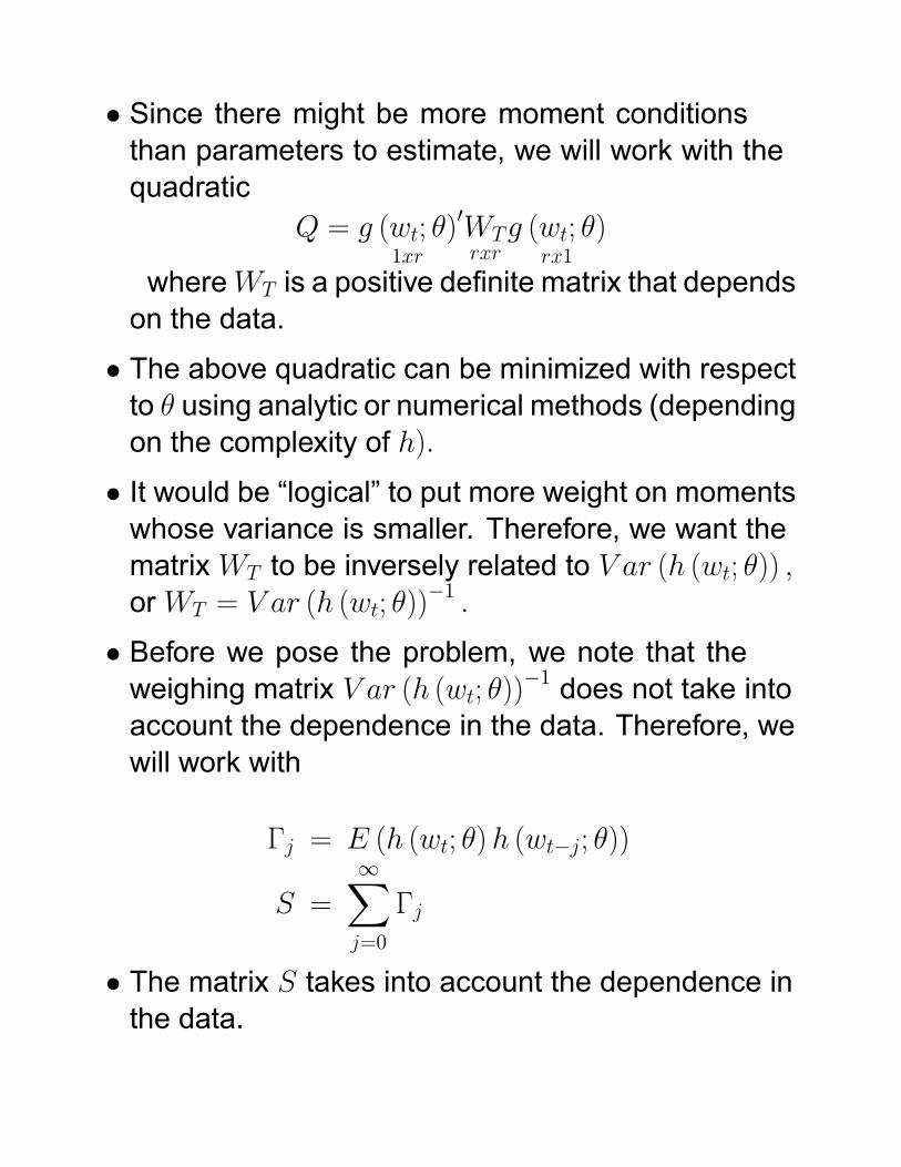
� Since there might be more moment conditionsthan parameters to estimate, we will work with thequadratic

Q = g (wt; �)1xr

0WTrxrg (wt; �)

rx1

whereWT is a positive de�nite matrix that dependson the data.

� The above quadratic can be minimized with respectto � using analytic or numerical methods (dependingon the complexity of h):

� It would be �logical� to put more weight on momentswhose variance is smaller. Therefore, we want thematrixWT to be inversely related to V ar (h (wt; �)) ;orWT = V ar (h (wt; �))

�1 :

� Before we pose the problem, we note that theweighing matrix V ar (h (wt; �))�1 does not take intoaccount the dependence in the data. Therefore, wewill work with

�j = E (h (wt; �)h (wt�j; �))

S =

1Xj=0

�j

� The matrix S takes into account the dependence inthe data.

� Long-run variance� 2� spectrum at frequency zero.

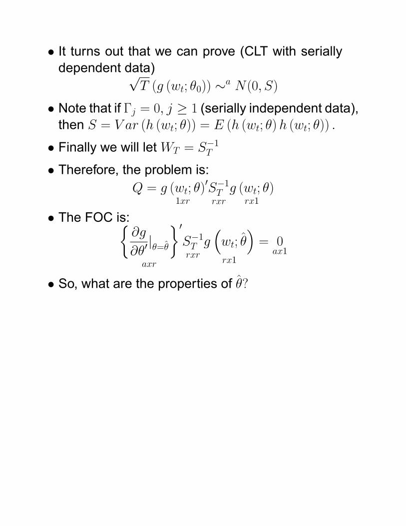
� It turns out that we can prove (CLT with seriallydependent data)p

T (g (wt; �0)) �a N(0; S)� Note that if �j = 0; j � 1 (serially independent data),then S = V ar (h (wt; �)) = E (h (wt; �)h (wt; �)) :

� Finally we will letWT = S�1T

� Therefore, the problem is:Q = g (wt; �)

1xr

0S�1Trxr

g (wt; �)rx1

� The FOC is:�@g

@�0j�=�

�axr

0S�1Trxr

g�wt; �

�rx1

= 0ax1

� So, what are the properties of �?

� Denote

D0

Trxa=

2664@g1(wt;�)@�0

@gr(wt;�)@�0

3775� We will show thatp

T�� � �0

��a N

�0;�DS�1D0��1�

� The �proof�' follows a few very simple steps� Use the Mean-Value theorem, to write

g�wt; �

�= g (wt; �0) +D

0T

�� � �0

�� Pre-multiply both sides by

n@g@�0j�=�

o0S�1T to get�

@g

@�0j�=�

�0S�1T g

�wt; �

�=

�@g

@�0j�=�

�0S�1T g (wt; �0) +

�@g

@�0j�=�

�0S�1T D

0T

�� � �0

�� But, we know by de�nition that�

@g

@�0j�=�

�0S�1T g

�wt; �

�= 0

� Or�@g

@�0j�=�

�0S�1T g (wt; �0) = �

�@g

@�0j�=�

�0S�1T D

0T

�� � �0

�� Rearranging, we get�

� � �0�

ax1

= D�1Taxr

g (wt; �0)rx1

� Then, pT�� � �0

�= D�1

T

pTg (wt; �0)

� But, recall thatpT (g (wt; �0)) �a N(0; S)

� Hence,pT�� � �0

�� aN(0; D�1

T SD�10T )

� aN

�0;�DTS

�1D0

T

��1�

� Final Result: The GMM estimates are asymp-totically normally distributed with a variance-covariance matrix equal to

�DTS

�1D0

T

��1=T

� This is a huge result. All we needed was a set ofmoment conditions, nothing else!

� We also need the data wt to be stationary.� Many �standard� problems can be written as GMM.� The real power of GMM is that one framework canhandle a lot of interesting problems.

It should be immediately obvious that the numberof orthogonality conditions and the conditioninginformation matter� In practice, the �type� of conditioning informationwill have a great impact on the estimates �: Thinkinstrumental variables.

� The question is: Which moments to choose?� This is quite discomforting. If slight variations in ourproblem yields widely different estimates of �; whatcan we conclude?

� Also: Estimating the matrix S makes a hugedifference. Recall that

�j = E (h (wt; �)h (wt�j; �))

S =

1Xj=0

�j

� Using sample analogues to obtain �j and S isnot the right way. Newey and West (1987) haveproposed a �corrected� way, which is:

S = �0 +

qXv=1

�1� v

q + 1

���j + �

0j

�� Even the Newey-West method does not yield goodresults when the dimension of the system is large.

� Moreover, the truncation point, q; introducesanother source of error.

� People have shown that small perturbations in Sresults in big differences in the estimates �. In otherwords, suppose we use a matrix

S + P

where P has small values on its diagonals(perturbing the variances only). This results inwidely different estimates. So, small differences inestimating S matter a lot.

� The mechanics of why this is so reside in takinginverses...

� Since we only need the optimal weighing matrixS for ef�ciency (smallest variance), is it possibleto �nd a matrix that, although not yielding ef�cientestimates, yields robust estimates?

� In practice: The best (most robust) results areobtained with I; the identity matrix.

� Empirical rule of thumb: Try the identity matrix �rst.Then, try the optimal weighing matrix, S: If theresults are widely different, stick with I:

In his 1982 seminal paper, L.P. Hansen arguedthat the multiplicity of the moments, or the over-identi�cations, are an advantage, rather than adisadvantage.� Even though we cannot have g

��; wt

�= 0; it must

be the case that at, and close to, the true value �0;g() will be close to zero.

� Note that, sincepT (g (wt; �0)) �a N(0; S)

then, it must be the case thatTg (wt; �0)

0 S�1g (wt; �0) �a????� It might be conjectured that the same would holdtrue for �; or that

Tg�wt; �

�0S�1g

�wt; �

��a �2 (r)

� However, this intuition is false, because it isnot necessarily the same linear combination ofg�wt; �

�that would be close to zero. Instead, it can

be shown thatTg�wt; �

�0S�1g

�wt; �

��a �2 (r � a)

� Note: This statistic is trivial to estimate. Plug � intog (:), etc.

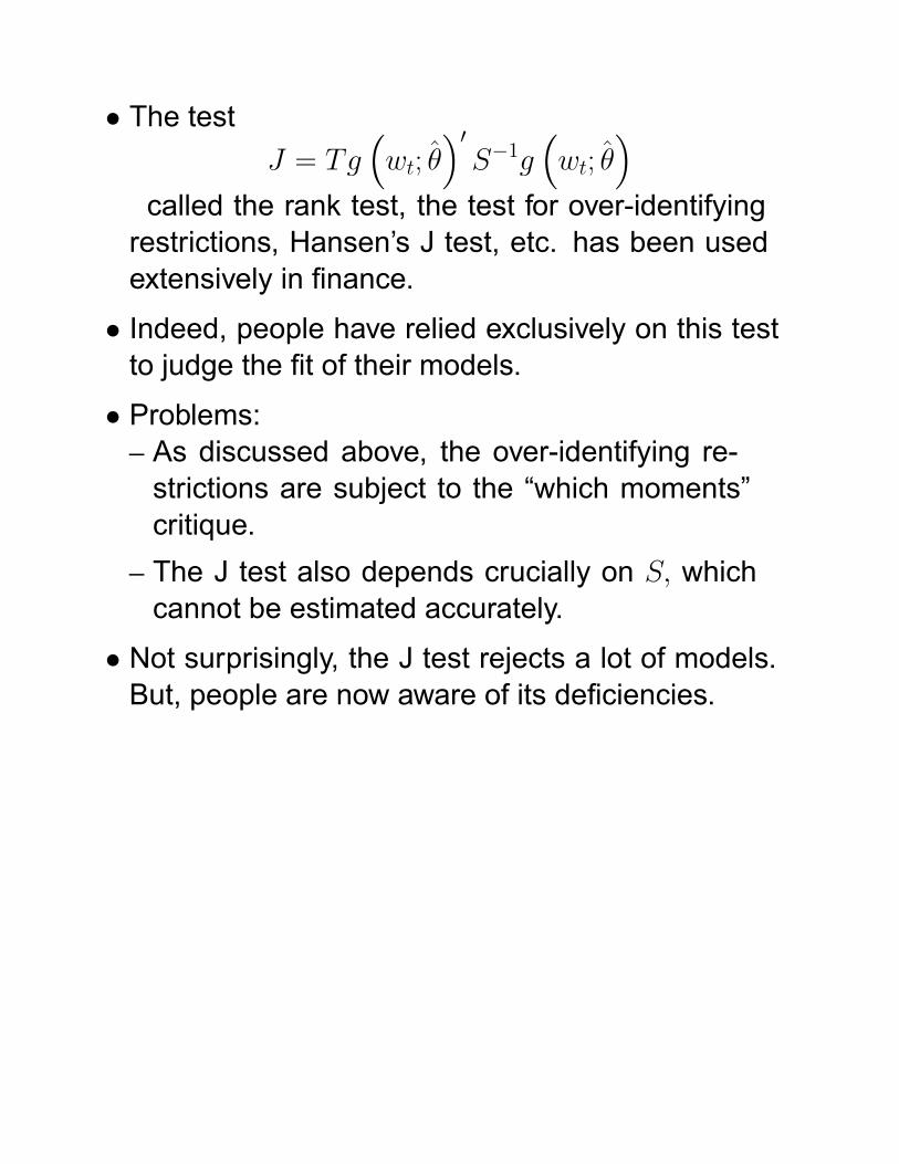
� The testJ = Tg

�wt; �

�0S�1g

�wt; �

�called the rank test, the test for over-identifyingrestrictions, Hansen's J test, etc. has been usedextensively in �nance.

� Indeed, people have relied exclusively on this testto judge the �t of their models.

� Problems:� As discussed above, the over-identifying re-strictions are subject to the �which moments�critique.

� The J test also depends crucially on S; whichcannot be estimated accurately.

� Not surprisingly, the J test rejects a lot of models.But, people are now aware of its de�ciencies.

� The GMM framework is rich enough that we canthink of many other ways of testing the hypothesesof interest. As a starting point, we can break theorthogonality restrictions into those that identify andthose that over-identify the parameters

E

�h1 (wt; �0)h2 (wt; �0)

�=

�00

�� Some people have suggested to see how the esti-mates would change as we add more restrictions toh2 (say, starting from no over-identifying restrictions,and adding progressively).

� This set-up has also yielded insights into thestability properties of the moments and (or versus)the estimates.

� Example (Hansen, EMA 1982; Hansen and Single-ton, EMA 1982):

pt = Et (m (ztj�)xt+1)� m (ztj�) is the stochastic discount factor thatdepends on some state variables and parameters.

� xt+1 is the payoff from the asset.� Example from last lecture:

pt = Et

"�

�ct+1ct

�� xt+1

#� We don't need to log-linearize anything with GMM.� Non-linearities are not a problem.� Robustness is a real issue.� But this is not what people use. Why?

� We can re-write the pricing equation as:

1 = Et

�m (ztj�)

xt+1pt

�Et (m (ztj�)Rt+1)� 1 = 0

where Rt+1 = xt+1=pt: In the case of stocks, thinkxt+1 = pt+1 + dt+1:

� In this case, returns are stationary.� If zt in the stochastic discount factor is alsostationary, then the ergoticity theorem conditionswill be satis�ed (under some other mild conditions).

� Example from last lecture:

Et

"�

�ct+1ct

�� (1 +Rt+1)

#� 1 = 0

� We have the data fct; Rtg:� Have to estimate one parameter, (assuming � is0.995).

3 Maximum Likelihood Estimation

(Preliminaries for Kalman Filtering)� Suppose we have the series fY1; Y2;::::; YTg witha joint density fYT ::::Y1(�) that depends on someparameters � (such as means, variances, etc.)

� We observe a realization of Yt.� If we make some functional assumptions on f; wecan think of f as the probability of having observedthis particular sample, given the parameters �:

� The maximum likelihood estimate (MLE) of � is thevalue of the parameters � for which this sample ismost likely to have been observed.

� In other words, �MLE is the value that maximizesfYT ::::Y1(�):

� Q: But, how do we know what f�the true density ofthe data�is?

� A: We don't.� Usually, we assume that f is normal, but this isstrictly for simplicity. The fact that we have to makedistributional assumptions limits the use of MLE inmany �nancial applications.

� Recall that if Yt are independent over time, thenfYT ::::Y1(�) = fYT (�T )fYT�1(�T�1):::fY1(�1)

= �Ti=1fYi (�i)

� Sometimes it is more convenient to take the log ofthe likelihood function, then

� (�) = log fYT ::::Y1(�) =TXi=1

log fYi (�)

� However, in most time series applications, theindependence assumption is untenable. Instead,we use a conditioning trick.

� Recall thatfY2Y1 = fY2jY1fY1

� In a similar fashion, we can writefYT ::::Y1(�) = fYT jYT�1::::Y1(�)fYT�1jYT�2::::Y1(�):::fY1(�)

� The log likelihood can be expressed as

� (�) = log fYT ::::Y1(�) =TXi=1

log fYijYi�1;:::;Y1 (�i)

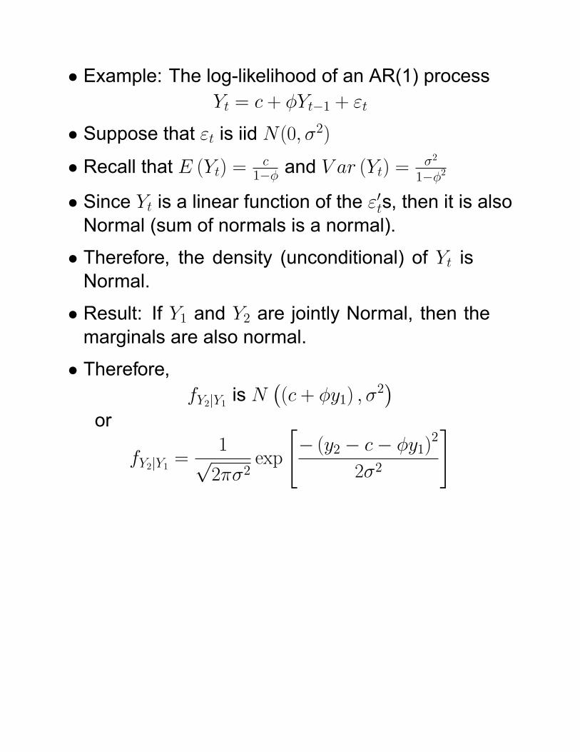
� Example: The log-likelihood of an AR(1) processYt = c + �Yt�1 + "t

� Suppose that "t is iid N(0; �2)� Recall that E (Yt) = c

1�� and V ar (Yt) =�2

1��2

� Since Yt is a linear function of the "0ts, then it is alsoNormal (sum of normals is a normal).

� Therefore, the density (unconditional) of Yt isNormal.

� Result: If Y1 and Y2 are jointly Normal, then themarginals are also normal.

� Therefore,fY2jY1 is N

�(c + �y1) ; �

2�

or

fY2jY1 =1p2��2

exp

"� (y2 � c� �y1)2

2�2

#

� Similarly,fY3jY2 is N

�(c + �y2) ; �

2�

or

fY3jY2 =1p2��2

exp

"� (y3 � c� �y2)2

2�2

#

Then,the log likelihood can be written as

� (�) = log fY1 +TXt=2

log fYtjYt�1

= �12log (2�)� 1

2log��2=

�1� �2

���fy1 � (c= (1� �))g

2

2�2=�1� �2

��(T � 1)

2log (2�)� (T � 1)

2log��2�

�TXt=2

(yt � c� �yt�1)2

2�2� The unknown parameters are collected in � =(c; �; �)

� We can maximize � (�) with respect to all thoseparameters and �nd the estimates that maximizethe probability of having observed such a sample.

max�� (�)

� Sometimes, we can even put constraints (such asj�j < 1)

� Q: Is it necessary to put the constraint �2 > 0?

� Note: If we forget the �rst observation, then we canwrite (setting c = 0) the FOC:

�TXt=2

@

@�

(yt � �yt�1)2

2�2= 0

TXt=2

yt�1 (yt � �yt�1) = 0

� =

PTt=2 yt�1ytPTt=2 y

2t�1

� RESULT: In the univariate linear regression case,OLS, GMM, MLE are equivalent!!!

� To summarize the maximum likelihood principle:(a) Make a distributional assumption about the data(b) Use the conditioning to write the joint likelihoodfunction

(c) For convenience, we work with the log-likelihoodfunction

(d) Maximize the likelihood function with respect tothe parameters

� There are some subtle points.� We had to specify the unconditional distribution ofthe �rst observation

� We had to make an assumption about thedependence in the series

� But sometimes, MLE is the only way to go.� MLE is particularly appealing if we know thedistribution of the series. Most other de�cienciescan be circumvented.

� Now, you will ask: What are the properties of�MLE

? More speci�cally, is it consistent? What is itsdistribution, where

�MLE

= argmax� (�)

� Yes, �MLE is a consistent estimator of �:� As you probably expect the asymptotic distributionof �

MLEis normal.

� Result:T 1=2

��MLE � �

�� aN (0; V )

V =

��@

2� (�)

@�@�0j�MLE

��1or

V =

TXt=1

l��MLE

; y�l��MLE

; y�

l��MLE

; y�=@f

@�

��MLE

; y�

� But we will not dwell on proving those properties.

Another Example: The log-likelihood of anAR(1)+ARCH(1) process

Yt = c + �Yt�1 + ut� where,

ut =phtvt

� ARCH(1) is:ht = � + au

2t�1

where vt is iid with mean 0; and E�v2t�= 1:

� GARCH(1,1): Suppose, we specify ht asht = � + �ht�1 + au

2t�1

� Recall that E (Yt) = c1�� and V ar (Yt) =

�2

1��2

� Since Yt is a linear function of the "0ts, then it is alsoNormal (sum of normals is a normal).

� Therefore, the density (unconditional) of Yt isNormal.

� Result: If Y1 and Y2 are jointly Normal, then themarginals are also normal.

� Therefore,fY2jY1 is N ((c + �y1) ; h2)

or for the ARCH(1)

fY2jY1 =1p

2� (� + au21)exp

"� (y2 � c� �y1)2

2 (� + au21)

#

� Similarly,fY3jY2 is N ((c + �y2) ; h3)

or

fY3jY2 =1p

2� (� + au22)exp

"� (y3 � c� �y2)2

2 (� + �u22)

#

Then,the conditional log likelihood can be writtenas

� (�jy1) =TXt=2

log fYtjYt�1

= �(T � 1)2

log (2�)� (1)2

TXt=2

log�� + au2t�1

��

TXt=2

(yt � c� �yt�1)2

2�� + �u2t�1

�� The unknown parameters are collected in � =(c; �; �; �)

� We can maximize � (�) with respect to all thoseparameters and �nd the estimates that maximizethe probability of having observed such a sample.

max�� (�)

� Example:mle_arch.m

� Similarly for GARCH(1,1):

� (�jy1) =TXt=2

log fYtjYt�1

= �(T � 1)2

log (2�)� (1)2

TXt=2

log (ht)

�TXt=2

(yt � c� �yt�1)2

2 (ht)

� whereht = � + �ht�1 + �u

2t�1

4 Kalman Filtering

� History: Kalman (1963) paper� Problem: We have a missile that we want to guideto its proper target.� The trajectory of the missile IS observable fromthe control center.

� Most other circumstances, such as weatherconditions, possible interception methods, etc.are NOT observable, but can be forecastable.

� We want to guide the missile to its properdestination.

� In �nance the setup is very similar, but the problemis different.

� In the missile case, the parameters of the systemare known. The interest is, given those parameters,to control the missile to its proper destination.

� In �nance, we want to estimate the parameters ofthe system. We are usually not concerned witha control problem, because there are very fewinstruments we can use as controls (although thereare counter-examples).

4.1 Setup (Hamilton CH 13)

yt = A0xt +H0zt + wt

zt = Fzt�1 + vtwhere

� yt is the observable variable (think �returns�)� The �rst equation, the yt equation is called the�space� or the �observation� equation.

� zt is the unobservable variable (think �volatility� or�state of the economy�)� The second equation, the zt equation is called the�state� equation.

� xt is a vector of exogenous (or predetermined)variables (we can set xt = 0 for now).

� vt and wt are iid and assumed to be uncorrelated atall lags

E (wtv0t) = 0

� Also E (vtv0t) = Q; E (wtw0t) = R� The system of equations is known as a state-spacerepresentation.

� Any time series can be written in a state-spacerepresentation.

� In standard engineering problems, it is assumedthat we know the parameters A;H; F;Q;R:

� The problem is to give impulses xt such that, giventhe states zt; the missile is guided as closely totarget as possible.

� In �nance, we want to estimate the unknownparameters A;H; F;Q;R in order to understandwhere the system is going, given the states zt:There is little attempt at guiding the system. In fact,we usually assume that xt = 1 and A = E(Yt); oreven that xt = 0:

� Note: Any time series can be written as a statespace.

� Example: AR(2): Yt+1 � � = �1 (Yt � �) +�2 (Yt�1 � �) + "t+1

� State equation:�Yt+1 � �Yt � �

�=

��1 �21 0

� �Yt � �Yt�1 � �

�+

�"t+10

�� Observation equation:

yt = � +�1 0

� � Yt+1 � �Yt � �

�� There are other state-space representations of Yt:Can you write down another one?

� As a �rst step, we will assume that A;H; F;Q;Rare known.

� Our goal would be to �nd a best linear forecast ofthe state (unobserved) vector zt: Such a forecastis needed in control problems (to take decisions)and in �nance (state of the economy, forecasts ofunobserved volatility).

� The forecasts will be denoted by:zt+1jt = E (zt+1jyt:::; xt::::)

and we assume that we are only taking linearprojections of zt+1 on yt:::; xt::::: Nonlinear KalmanFilters exist but the results are a bit more compli-cated.

� The Kalman Filter calculates the forecasts zt+1jtrecursively, starting with z1j0; then z2j1; ...until zT jT�1:

� Since ztjt�1 is a forecast, we can ask how good of aforecast it is?

� Therefore, we de�ne Ptjt�1 = E��zt � ztjt�1

� �zt � ztjt�1

��;

which is the forecasting error from the recursiveforecast ztjt�1:

� The Kalman Filter can be broken down into 5 steps1. Initialization of the recursion. We need z1j0: Usually,we take z1j0 to be the unconditional mean, orz1j0 = E (z1) : (Q: how can we estimate E (z1)? )The associated error with this forecast is P1j0 =E��z1j0 � z1

� �z1j0 � z1

��

2. Forecasting yt (intermediate step)The ultimate goal is to calculate ztjt�1, but we dothat recursively. We will �rst need to forecast thevalue of yt; based on available information:

E (ytjxt; zt) = A0xt +H 0ztFrom the law of iterated expectations,

Et�1 (Et (yt)) = Et�1 (yt) = A0xt +H

0ztjt�1The error from this forecast is

yt � ytjt�1 = H 0 �zt � ztjt�1� + wtwith MSE

E�yt � ytjt�1

� �yt � ytjt�1

�0= E

hH 0 �zt � ztjt�1� �zt � ztjt�1�0Hi + E [wtw0t]

= H 0Ptjt�1H +R

3. Updating Step (ztjt)� Once we observe yt; we can update our forecastof zt; denoting it by ztjt; before making the newforecast, zt+1jt:

� We do this by calculating E (ztjyt; xt; :::) = ztjtztjt = ztjt�1 + E

��zt � ztjt�1

� �yt � ytjt�1

����

E�yt � ytjt�1

� �yt � ytjt�1

�0��1 �yt � ytjt�1

�� We can write this a bit more intuitively as:

ztjt = ztjt�1 + ��yt � ytjt�1

�where � is the OLS coef�cient from regressing�zt � ztjt�1

�on�yt � ytjt�1

�:

� The bigger is the relationship between the twoforecasting errors, the bigger the correction mustbe.

� It can be shown thatztjt = ztjt�1+Ptjt�1H

�H 0Ptjt�1H +R

��1 �yt � A0xt �H 0ztjt�1

�� This updated forecast uses the old forecast ztjt�1;and the just observed values of yt and xt.

4. Forecast zt+1jt:� Once we have an update of the old forecast, wecan produce a new forecast, the forecast of zt+1jt

Et (zt+1) = E (zt+1jyt; xt; :::)= E (Fzt + vt+1jyt; xt; :::)= FE (ztjyt; xt; :::) + 0= Fztjt

� We can use the above equation to writeEt (zt+1) = Ffztjt�1

+Ptjt�1H�H 0Ptjt�1H +R

��1 �yt � A0xt �H 0ztjt�1

�g

= Fztjt�1

+FPtjt�1H�H 0Ptjt�1H +R

��1 �yt � A0xt �H 0ztjt�1

�� We can also derive an equation for the error inforecast as a recursionPt+1jt = F [Ptjt

�Ptjt�1H�H 0Ptjt�1H +R

��1H 0Ptjt�1]F

0

+Q

5. Go to step 2, until we reach T. Then, we are done.

� Summary: The Kalman Filter produces� The optimal forecasts of zt+1jt and yt+1jt (optimalwithin the class of linear forecasts)

� We need some initialization assumptions� We need to know the parameters of the system,i.e. A; H; F; Q; R:

� Now, we need to �nd a way to estimate theparameters A; H; F; Q; R:

� By far, the most popular method is MLE.� Aside: Simulations Methods�getting away from therestrictive assumptions of "t

4.2 Estimation of Kalman Filters (MLE)

� Suppose that z1; and the shocks (wt; vt) are jointlynormally distributed.

� Under such an assumption, we can make the verystrong claim that the forecasts zt+1jt and yt+1jtare optimal among any functions of xt; yt�1:::: Inother words, if we have normal errors, we cannotproduce better forecasts using the past data thanthe Kalman forecasts!!!

� If the errors are normal, then all variables in thelinear system have a normal distribution.

� More speci�cally, the distribution of yt conditionalon xt, and yt�1; ::: is normal, orytjxt; yt�1::: � N

�A0xt +H

0ztjt�1;�H 0Ptjt�1H +R

��� Therefore, we can specify the likelihood function ofytjxt; yt�1 as we did above.

fytjxt;yt�1 = (2�)�n=2��H 0Ptjt�1H +R

���1=2� exp[�1

2

�yt � A0xt �H 0ztjt�1

�0 �H 0Ptjt�1H +R

��1��yt � A0xt �H 0ztjt�1

�]

� The problem is to maximize

maxA;H;F;Q;R

TXt=1

log fytjxt;yt�1

� Words of wisdom:� This maximization problem can easily get un-manageable to estimate, even using moderncomputers. The problem is that searching forglobal max is very tricky.� A possible solution is to make as many restric-tions as possible and then to relax them one byone.

� A second solution is to write a model that givestheoretical restrictions.

� Recall that there are more than 1 state spacerepresentations of an AR process. This impliesthat some of the parameters in the state-spacesystem are not identi�ed. In other words, morethan one value of the parameters (differentcombinations) can give rise to the same likelihoodfunction.� Then, which likelihood do we choose?� Have to make restrictions so that we have anexactly identi�ed problem.

Applications in Finance� Anytime we have unobservable state variables(Brandt et al. (2005))

rt+1 = a + b�t + et+1�t = � + ��t�1 + wt

� Interpolation of data (Bernanke (1989))� Time varying parameters (Stock and Watson(1996)):

rt+1 = � + �txt + et+1�t = � + ��t�1 + vt

5 Non-linear Dependence

� In �nance, the characterization of the variation ofreturns and the dependence between returns iscrucial.

� Thus far, the variation has been captured by thevariance.

� The dependence has been captured by the covari-ance.

� The covariance is a good measure only with linearmodels.

� Non-linear dependence needs to be addressed.� Suppose we have two assets R and F with returnsRS and RF whose distribution is FRS and FRF :

� The �complete� behavior is de�ned by their distribu-tions.

� We might want to know how the entire distributionof the two variables. In other words, we want toknow the joint distribution, FRS,RF :

� Q: Why?� A: Because there might be nonlinearity in therelation between the two variables.

� Find a general way of relating the two distributions,FRS and FRF

� For instance, how would the tails of the distributionschange during extreme events? More? Less?� With credit derivatives, suppose that the creditrating of the underlying (Bond) changes.

� Or, can we model the dependence non-linearly?� Would we see skewness, kurtosis, etc.?� There is a lot of interest in the profession in �ndingadequate (alternative) measures of dependencethat go beyond simple correlations.

� There are two (three) main ways to go:� Copulas� Tail dependence� Quantile Regressions

� These are different approaches at modeling thenon-linear dependence between the distributionsFRS and FRF

5.1 Copulas

The problem is as follows. Find a general way ofrelating the two distributions, FRS and FRF in order to�nd the joint distribution FRS,RF :� In other words, we want to do the following

FRS,RF = C (FRS; FRF )

where C(:; :) is some appropriately chosen function.

� The goal is to choose the right C(:; :):

� Note: We cannot choose any C(:; :):There aresome restrictions that are imposed by the fact thatwe are dealing with distributions.

� Simple example; C(x; y) = x:y� Q: When is this copula appropriate?

� Another example: C(x; y) = min(x; y)� Another example: C(x; y) = N�

�N�1 (x) ; N�1 (y)

�where � is the correlation.

� Two widely used copulas:� Gumbel's bivariate exponential:C� (x; y) = x + y � 1 + (1� x) (1� y) e�� ln(1�x)(1�y)where � measures the non-linear dependence.For � = 0; we have

C�=0 (x; y) = x:y

� AMH Copulas (Ali-Mikhail-Haq):C� (x; y) =

xy

1� � (1� x) (1� y)where � measures the non-linear dependence.For � = 0; we have

C�=0 (x; y) = x:y

� In general, if you work with copulas:� You want to �nd a �exible form for C(.,.)� You want to be able to estimate all the depen-dence parameters.

5.2 Tail dependence

The main question is as follows. What is the proba-bility that we will have an extreme (tail) realization ofRF given that we observe an extreme tail realizationof RS?� Note: We are not looking at typical co-movements(covariance) but at tail co-movements?

� A natural de�nition of tail dependence is:� On the positive side:

�+ = Pr (RS > extreme positive value j RF > extreme positive value)= lim

u!1�Pr�RS > F

�1Rs(u) jRF > F�1RF (u)

�� On the negative side:

�� = Pr (RS < extreme negative value j RF > extreme negative value)= lim

u!0Pr�RS < F

�1Rs(u) jRF < F�1RF (u)

�

� I.e., what is the chance of observing a very positive(negative) return in the underlying asset, given thatwe have observed a very positive (negative) returnin the hedging asset.

� Instead of average dependence, we are looking attail dependence.

� Intuitively, copulas and tail dependence are related.� There are also mathematical connections betweenthe two:

�+=limu!11�2u+C(u;u)

1�u

�� = limu!0

C (u; u)

u� For instance, for the Gumbel's copula

�+ = 1� 2�

� Note: �+ = 0 means no tail dependence (when� = 0). But the distributions might be otherwisedependent.

5.3 Quantile regression:

� Model the conditional quantiles of the distribution� Instead of

RF = � + �RS + "where we model the conditional mean, we want tomodel the conditional quantiles.

� We do that by specifying:QRF (� ) = � (� ) + � (� )RS + "

for � between 0 and 1 where QRF (� ) is the �quantile of RF :

� Recall the de�nition of a quantile: (inverse ofdistribution).

� This is called a quantile regression, because weare modeling the quantiles of the distribution.� For � = 0:5, we are estimating how the median ofthe distribution of RF depends on RS:

� Similarly, for � = 0:05 or � = 0:99; we are estimat-ing the extreme quantiles of the distribution.

� Quantile regressions are easy to estimate (similarto OLS).

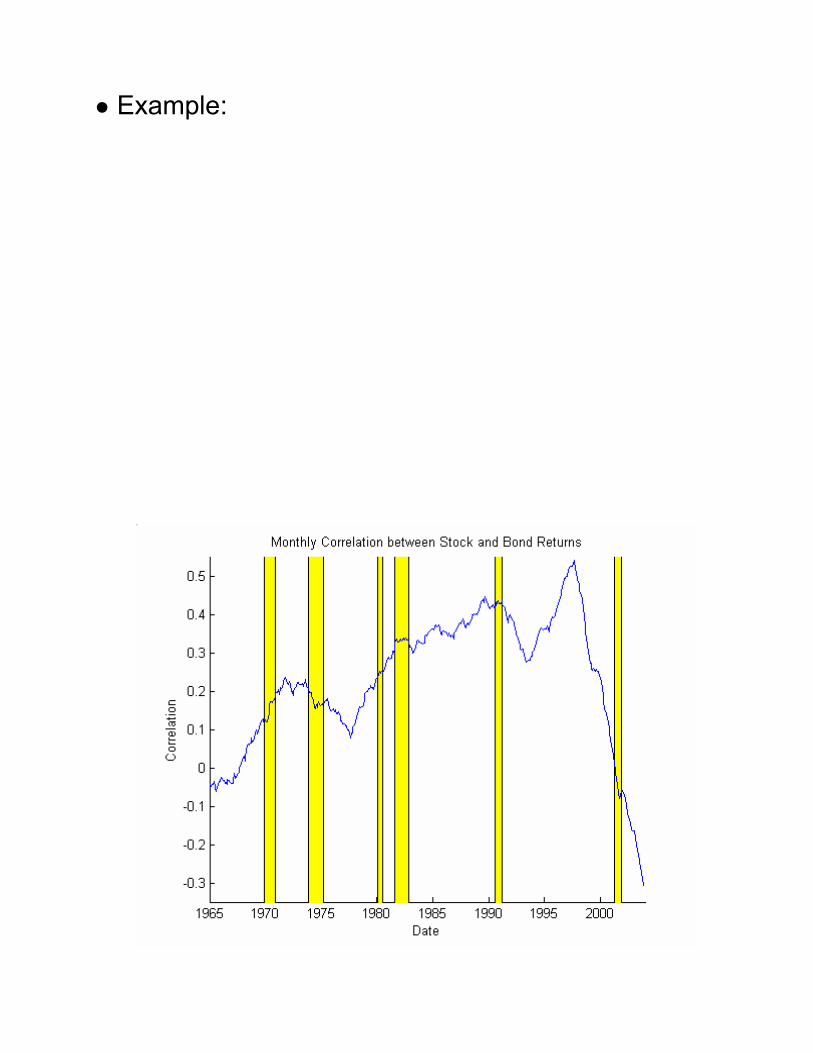
� Example: