Today in Astronomy 111: rings, gaps and orbits

8 November 2011 Astronomy 111, Fall 2011 1

Today in Astronomy 111: rings, gaps and orbits

Cassini/JPL/ NASA

Pan Dione

Titan

Pandora

Encke KeelerF

A

Gap sizes: the Hill radius Perturbations and resonances The variety of structures in planetary rings

• Spiral density waves• Bending waves • Horseshoe and

tadpole orbits• Shepherding

Perturbations and

the measurement of planetary/satellite moments of inertia.

http://saturn.jpl.nasa.gov/photos/


The Hill radius

As before, in a coordinate system revolving with a satellite or planet, the effective gravitational acceleration due to the parent body is

and, at the location of the satellite,and in the radial direction, is

2 3effGM GMg rr a

= − +

( ) 3 3

3

2

3

effp

dg GM GMg r a rdr a a

GM ra

= ∆ = + ∆

= ∆

a

∆r

m

M

a

∆r

m

M

The Hill radius (continued)

Along the radial direction from the parent body, the gravitational acceleration due to the satellite isso the magnitudes of acceleration areequal at a distance from the satellitegiven by

This is (half) the range of orbital radii sweptout by the satellite’s gravitational sphere of influence: within this range, thesatellite perturbs the orbits of otherbodies very strongly.


2 ,sg Gm r= − ∆

1 3

3 23 .

3HGM Gm mr r r a

Ma r ∆ = ⇒ = ∆ = ∆


The Hill radius (continued)

Example: A spherical body with diameter 7 km and density 1 gm cm-3 (icy, like Saturn’s ring particles), 136530 km away from Saturn (like the Keeler gap), has a Hill radius of 6.5 km, so this body should perturb the orbits of smaller ones, and clear a gap at least twice as big around as the body.

Which is just about right.

Cassini image of the Keeler gap and the satellite S/2005 S1;JPL/NASA.

http://saturn.jpl.nasa.gov/photos/


Orbital perturbations

As we have learned, in the simple case of transfer orbits, exerting forces or impulses (momentum changes) on satellites changes their orbits in straightforwardly-predictable ways.Of course, straightforward here does not mean simple.

Depending upon where in the orbit an impulse is applied, and in what direction, various of the orbital parameters can be changed, and in general all change.

The form of the equations of motion, though, can be used to identify points at which the impulse affects just one or two of the orbital parameters.

See CS table 11.3 (page 225) for the formulas in full regalia, but we won’t be using them…


A guide to perturbations

The only perturbative impulses we have considered hitherto have been transverse accelerations: those in the plane of the orbit, perpendicular to the radius.

Increases a, small change in ε, slows down orbit

At apoapse: increases a, decreases ε.

At periapse: increases a and ε.

Increases a, small change in ε, speeds up orbit


A guide to perturbations (continued)

Normal accelerations (i.e. perpendicular to the initial orbital plane) change the inclination and precession rate.

Applied here, precessesorbital plane counterclockwise.

Applied here, precesses orbital plane clockwise.

Applied at periapse, increases orbital inclination

Applied at apoapse, decreases orbital inclination


A guide to perturbations (continued)

Radial accelerations are rather counterintuitive around periapse and apoapse.

Applied here, aand ε increase.

Applied here, aand ε decrease.

Applied at periapse: no change in a or ε;satellite speeds up in orbit.

Applied at apoapse: no change in a and ε; satellite slows down in orbit.


Orbital resonances and waves

If perturbations take place periodically (i.e. at regular intervals), then their effects can build over time as a series of them can “add constructively.”• Periodic normal perturbations can drive vertical

oscillations in the orbits of small bodies: simple harmonic motion, with the gravity of the disk of ring particles (and the vertical component of the planet’s gravity) acting as the restoring force.

• Radial perturbations can drive radial oscillations, which, combined with revolution, cause bodies to travel in circles with their centers in uniform Keplerian motion (epicycles).


Orbital resonances and waves

If at a certain location for which the orbital angular frequency is Ω, the natural angular frequency of vertical oscillations is ν and that of radial oscillations is κ, and the angular frequency at which the perturbation occurs is Ωp, then the perturbation is resonant if

These general, multimode resonances are usually called Lindblad resonances by astronomers.

Waves are patterns in the structure (density or position) created by orbital resonances.

( )0 , , , integersph i j k h i j kν κ+ + Ω + Ω ≈


Spiral density waves

There are many resonances very near each satellite.Oscillations are damped as a function of distance from the

satellite. The waves when damped put angular momentum into

the disk. This moves material away from the satellite, where it can pile up with material that was already there: a wave in the density of the ring particles.


Bending waves

The same reasoning applies to vertical oscillations; the result is a ripple-shaped bending of the ring-disk. Saturn’s rings are very thin. They are resolved in the

vertical direction only because they carry bending waves. Amplitudes of the bending waves can be thousands of

times larger than the ring thickness.


Waves in Saturn’s rings

This Voyager image captured a closeup of a pair of waves at the 5:3 resonance with the moon Mimas. The inner wave (right) is a spiral bending wave, made of vertical positional oscillations and azimuthal density oscillations in the rings. It is visible because the peaks cast shadows over the troughs. The outer wave (left) is a spiral density wave, in which particles are bunched together in a spiral pattern due to azimuthal density oscillations.

http://voyager.jpl.nasa.gov/


Spiral density waves in Saturn’s A ring

Each set of waves is driven by Mimas(probably) at a different j and k (Cassini/JPL/ NASA).

http://saturn.jpl.nasa.gov/multimedia/images/images.cfm?categoryID=5


Horseshoe and tadpole orbits

Particles perturbed by a satellite, or even a pair perturbed by each other, can find themselves in orbits closely associated with the two-body potential and the five Lagrange points.Orbits around L4 and L5, if large enough, elongate

parallel to the potential contours; these are called tadpole orbits.

Orbits can enclose L3, L4, and L5, in which case they are called horseshoe orbits, famously exemplified by Janus and Epimetheus.

JanusEpimetheus

Cassini/JPL/NASA

http://photojournal.jpl.nasa.gov/catalog/PIA08348

http://photojournal.jpl.nasa.gov/catalog/PIA08348


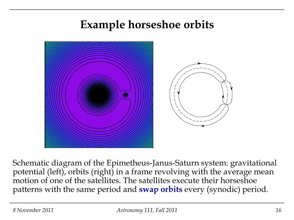
Example horseshoe orbits

Schematic diagram of the Epimetheus-Janus-Saturn system: gravitational potential (left), orbits (right) in a frame revolving with the average mean motion of one of the satellites. The satellites execute their horseshoe patterns with the same period and swap orbits every (synodic) period.


Example horseshoe orbits (continued)

Nice simulations of the Janus-Epimetheus system on Robert Vanderbei’s website: click here. Ideal horseshoe orbit in a revolving reference frame at rest

with respect to Saturn and either J or E (cf. the previous page): choose Ideal Epimetheus/Janus (and Start).

Realistic horseshoe J-E orbits: choose ephemeris Epimetheus/Janus (and Start). Note that the orbital motion is no longer smooth.

Initial tadpole orbit (two moons with J/E properties, one of which starts on the other’s L4 or L5 point): choose Epimetheus/Janus at L4/L5.

Non-revolving reference frame: see this page by S. Edgeworth.

http://www.princeton.edu/~rvdb/

http://www.princeton.edu/~rvdb/

http://www.princeton.edu/~rvdb/JAVA/astro/galaxy/Janus0.html

http://www32.brinkster.com/snefru/space/twin/


Shepherding and shepherd satellites

If two satellites orbit at similar radii, their orbital resonances can trap particles and drive density waves in the annulus between their orbits. This confinement is called shepherding. Lots of the fine-scale structure in the Saturn ring system is

due to multiple small satellites with closely-spaced, nested orbits, shepherding the material in between.

The rings so shepherded will show prominently the density-wave structure driven by their shepherds, resulting in “ripples” and “braids” such as those seen in Saturn’s F ring.


Shepherd satellites (continued)

F ring

JanusPandora

Prometheus

Cassini/ JPL/ NASA



Structure in the F ring

Prometheus

(Cassini/JPL/NASA)



Perturbations and moment of inertia

The derivations, and results, of formulas for gravitational potential energy and moment of inertia are similar. For instance, for uniform density spheres,

(see the following, and the lecture notes for 20 September.) The similarity between gravitational potential energy and

moment of inertia persists for not-quite-spherical bodies, and provide us a means to measure the moment of inertia of a body – uniform or differentiated – by measurement of the details of the body’s gravitational field.

= − =2

23 2, .5 5

GMU I MRR


Gravitational potential energy of a uniform-density sphere

Suppose a uniform-density planet were made by collecting a mass M, originally in the form of small particles lying at r = infinity. Consider the point at which a spherical mass m had been built up within a radius and consider adding an infinitesimal increment dm:

33

2 3

2 23

2 32

2 2 3 30 0 0

4, where and3

3sin sin , so4

3 sin4

R r

Gmdm rdU d dr m r Mr R

Mdm r dr d d r dr d dR

Gmdm G r MU dr M r drdr d dr r R R

π π

ρ π

ρ θ θ φ θ θ φπ

θ θ φπ

′

∞

′′= ⋅ = = =

′ ′ ′ ′= =

′ ′ ′= = ∫ ∫ ∫ ∫ ∫ ∫

F

,r′

Gravitational potential energy of a uniform-density sphere (continued)

Most of the terms can be brought outside the various integrals:


( )

225

6 20 0 0

2

00 0

2

55 4

20 0

3 sin4

2 , sin cos 1 1 2

1 1 , so

5

R r

r r

R r R

GM drU d d dr rR r

d d

drr rr

dr Rdr r dr rr

π π

π ππ

φ θ θπ

φ π θ θ θ

′

∞

′ ′

∞∞′

∞

′ ′=

= = − = − − − =

= − = −′

′ ′ ′ ′= − = −

∫ ∫ ∫ ∫

∫ ∫

∫

∫ ∫ ∫

Gravitational potential energy of a uniform-density sphere (continued)

So


225

6 20 0 0

2 5

6

2

3 sin4

3 2 254

3 .5

R rGM drU d d dr rR r

GM RRGM

R

π πφ θ θ

π

ππ

′

∞

′ ′=

= ⋅ ⋅ ⋅

= −

∫ ∫ ∫ ∫A multivariable integral, though a simple one.


Describing gravity from a bumpy body, mathematically

It is possible, and convenient, to describe the gravitational potential Φ (potential energy per unit orbiting mass) of a bumpy body as the sum of a series of regular, smooth functions. For instance:

The conventional family of functions people use, depicted here, is the set of Legendre polynomials,of different order n, expressed as functions of

= + 0.1 + 0.1 + 0.1

( )θcos ,nPθcos :

( ) ( ) ( ) ( )( )θ φ θ θ θΦ = − + + +2 3 4, , 1 0.1 cos 0.1 cos 0.1 cosGMr P P Pr


Describing gravity from a bumpy body, mathematically (continued)

In the most general case, this is written as an infinite sum of Legendre polynomials, each with their own factor, expressing the magnitude of their contribution to the total:

where is the radius of the body at the equator. Don’t worry about the hieroglyphics; we’re not going to

be using this formula except as a substitute for the “sum of pictures” on the previous page.)

Legendre polynomials are called “zonal harmonics” in the textbook.

,nJ

( ) ( )2

, , 1 cos ,n

en n

n

RGMr J Pr r

θ φ θ∞

=

Φ = − −

∑

eR



Now, if we put a satellite in orbit around this bumpy body, that orbit will not be perfectly elliptical or constant. Instead, its orbit will be perturbed whenever it passes close to one of the “bumps.” Usually the biggest bump is the first term in the infinite series, with The orbit may precess, or have its semimajor axis,

eccentricity, or orientation change with time. If we measure the rates that these changes take place, we

can determine where and how large the perturbations are. This in turn can be used to work out what all the

( )θ2 2 and cos .J P

s are.nJ



It turns out that for bodies in hydrostatic equilibrium,

where H (not to be confused with the isothermal scale height!), a quantity called the dynamic ellipticity, can also be determined from the rate of precession of the satellite’s orbit. Thus

where all of the quantities on the right-hand side can be determined from the details of the satellite’s orbit: thus the moment of inertia of the body is derived from its gravity.

⊥ ⊥− −= = =2 2 2 2

e e e

I I I I I IJ HIMR MR MR

= 22 ,eJI MRH

Moment of inertia about an axis perpendi-cular to its normal rotation axis.



It is easiest to understand how this works for the case of an actual satellite making complete orbits around an actual planet, moon or asteroid, and indeed our best measurements of I come from orbiting deep-space probes.

But it is not necessary for the “orbit” to be a complete or closed orbit. Many of the measured I for asteroids come from the details of very precise and accurate measurements of trajectory and velocity for the asteroid as it encounters a satellite that’s just passing by, or even as it encounters another solar-system object, like Mars or its moons.

Documents

Today in Astronomy 111: rings, gaps and orbits