Embed Size (px)
Citation preview

N A S A
00
0 M
*o
d
4 cn 4 z
TECHNICAL NOTE
COULOMB CORRECTIONS TO THE BETHE-HEITLER CROSS SECTIONS FOR ELECTRON-NUCLEUS BREMSSTRAHLUNG
by S. H. Morgan, Jr.
George C. MmshalZ Space FZight Center Marshall Space FZight Center, A h . 35812
N A T I O N A L A E R O N A U T I C S A N D S P A C E A D M I N I S T R A T I O N W A S H I N G T O N , D. C. O C T O B E R 1970
i
https://ntrs.nasa.gov/search.jsp?R=19710001524 2020-06-03T11:04:41+00:00Z

TECH LIBRARY KAFB, NM
. .
6
1. Report No. "
I 2. Government Accession No.
NASA TN D-6038 4. Title and Subtitle
Coulomb Corrections To The Bethe-Heitler Cross Sections For Electron-Nucleus Bremsstrahlung
7. Author(s)
S. H. Morgan, Jr. " ~- . ."
9. Performing Organization Name and Address . " - ~~
George C. Marshall Space Flight Center Marshall Space Flight Center, Alabama 35812
1. . . __ 12. Sponsoring Agency Name and Address
. OL32b77 ~~
3. Recipient's Catalog No.
5. -Report Date October 1970
6. Performing Organization Code
'8. Performing Organization Report No.
10. Work Unit No. ~~ -~
M436 "
11. Contract or Grant No.
i3. Type of.Rep?rt and.Pericd Covered ~ " "
Technical Note 14. Sponsoring Agency Code
" . ".
". .
15. Supplementary Notes " ". - . ~
Prepared by Space Sciences Laboratory, Science and Engineering Directorate
. . - - ~.
16. Abstract " ~~ - - . . " ~~~ ."
The bremsstrahlung differential cross section is obtained using both the Born approximation and a partial wave expansion. The cross sections are evaluated for energies in the 0.2- and 2.0-MeV range and compared with the experimental results for different scattering media. A comparison is made between the two theoretical approaches to obtain a correction to the Born approximation. The corrected Born approximation gives relatively good results in the 0. I- to 2.0-MeV range but is not applicable to higher energies.
I I 17. Key Words (Suggested by Author(s)l " " - -
Bremsstrahlung differential cross section Born approximation Part ia l wave expansion Electron interactions 1
. " ~ ___ 18. Distribution Statement
"~ . . ~ _ _
Unclassified - Unlimited
I . .. ~~ . __ Security Classif. (of this report)
Unclassified Unclassified I 20. Security Classif. (of this page)
-. . . . " . . - .. ~ T"
*For sale by the Clearinghouse for Federal Scientific and Technical Information Springfield. Virginia 22151
p


TABLE OF CONTENTS
I
SECTION I.
SECTION 11.
SECTION 111.
SECTION IV.
SECTION V.
APPENDIX A:
APPENDIX B:
APPENDIX C:
Page
SUMNIARY ............................ 1
INTRODUCTION ......................... i
THEORY.. . ........................... 4
A. The General Bremsstrahlung Problem . . . . . . . 4 B. Cross Section for Bremsstrahlung
Production. . . . . . . . . . . . . . . . . . . . . . . . . . 8 C. The Bethe-Heitler Formulation of the
Bremsstrahlung Problem . . . . . . . . . . . . . . . . 1 i D. The Bremsstrahlung Problem Using
Coulomb Wave Functions . . . . . . . . . . . . . . . . 36
CROSS SECTION RESULTS . . . . . . . . . . . . . . . . . 57
COULOMB CORRECTION FACTOR. . . . . . . . . . . . 63
A. Extension of the Elwert Factor . . . . . . . . . . . . 63 B. Alternative Forms . . . . . . . . . . . . . . . . . . . . 66 C. Comparison with Experimental Cross
Sections . . . . . . . . . . . . . . . . . . . . . . . . . . . 6 9
SUMNIARY AND CONCLUSIONS . . . . . . . . . . . . . . 73
ELWERT COULOMB CORRECTION FACTOR FOR LOW ENERGIES . . . . . . . . . . . . . . . . . . . . . 75
NORMALIZATION O F THE RADIAL WAVE FUNCTIONS . . . . . . . . . . . . . . . . . . . . . . . . . . . 79
THE DIRAC EQUATION I N POLAR COORDINATES . . . . . . . . . . . . . . . . . . . . . . . . . 83
REFERENCES . . . . . . . . . . . . . . . . . . . . . . . . . . 98
iii

LIST OF TABLES
Table Title Page
I.
Figure
I.
2.
3.
4.
5.
6.
7 .
8.
The Approximate Relative Error of the Bethe-Heitler Theory When Compared to the Partial Wave Results . . . . . . 6 3
LIST OF ILLUSTRATIONS
Title Page
Geometry of the bremsstrahlung problem . . . . . . . . . . . . . . 5
Feynman diagram used to interpret the amplitude factors in the matrix element for a free particle- photon interaction [ 121 . . . . . . . . . . . . . . . . . . . . . . . . . . 12
Feynman diagrams for bremsstrahlung production [ 121 . . . . . . . . . . . . . . . . . . . . . . . . . . . . . . . 16
Amplitude of the radial function in the atomic form factor . . . . . . . . . . . . . . . . . . . . . . . . . . . . . . . . . . 33
Comparison of maximum impact parameter and radius of Thomas-Fermi atom for beryllium, aluminum, and gold . . . . . . . . . . . . . . . . . . . . . . . . . . . . 35
Bremsstrahlung cross sections differential in photon energy for 0.2 MeV electrons incident on aluminum, copper, tin, and gold . . . . . . . . . . . . . . . . . . . . . . . . . . . 58
Bremsstrahlung cross sections differential in photon energy for 0.5 MeV electrons incident on aluminum, copper, tin, and gold . . . . . . . . . . . . . . . . . . . . . . . . . . . 59
Bremsstrahlung cross sections differential in photon energy for I. 0 MeV electrons incident on aluminum, copper, tin, and gold . . . . . . . . . . . . . . . . . . . . . . . . . . . 60
iv

LIST OF ILLUSTRATIONS (Concluded)
Figure Tit le Page
9. Bremsstrahlung cross sections differential in photon energy for I. 7 MeV electrons incident on aluminum, copper, tin, and gold . . . . . . . . . . . . . . . . . . . . . . . . . . 61
i o . Schematic representation of screening and Coulomb regions . . . . . . . . . . . . . . . . . . . . . . . . . . . . . . . . . . . 64
1i. The ratio of the differential cross sections calculated by the partial wave method to the Bethe-Heitler theory. . . . 66
12. Extension of the Elwert factor to higher energies for incident electron energies - of 0.2 and 0.5 MeV, incident on gold .... 67
13. Comparison of calculated to actual correction fac tor . . . . . . . . . . . . . . . . . . . . . . . . . . . . . . . . . . . . . 68
14. Comparison of Bethe-Heitler and corrected differential cross sections for 0.2, 1. 0 , i. 7, and 2 . 5 MeV electrons incident on gold . . . . . . . . . . . . . . . . . . . . . . . . . . . . . . 70
15. Comparison of Bethe-Heitler and corrected differential cross sections for 0.2, 1.0, i. 7, and 2.5 electrons incident on t i n . . . . . . . . . . . . . . . . . . . . . . . . . . . . . . . 7 1
16. Comparison of Bethe-Heitler and corrected differential cross sect ions for 0 .2 , I. 0, I. 7, and 2.5 MeV electrons incident on aluminum . . . . . . . . . . . . . . . . . . . . . . . . . . 72
A-I ( a ) . Elwert Coulomb correction factor - effect of atomic number and photon energy on magnitude of correction . . . . 76
A - i ( b ) . Elwert factor for 0 . 3 MeV incident electrons as a function of photon fractional energy. . . . . . . . . . . . . . . . . 76
A-2. Effect of Elwert factor on bremsstrahlung cross sections for 0.2 MeV eiectrons incident on aluminum, copper, and gold . . . . . . . . . . . . . . . . . . . . . . . . . . . . . . . . . . . . . . 77
V

COULOMB CORRECTIONS TO THE BETHE-HEITLER CROSS SECTIONS FOR ELECTRON-NUCLEUS BREMSSTRAHLUNG
SUMMARY
The electron-nucleus bremsstrahlung cross section is computed by using the closed analytic expression for the Born approximation and a more elaborate calculation based upon a partial wave expansion. Theoretical details and a comparison of the results obtained by the two methods are presented.
A correction factor based upon the two methods is obtained. This factor is then used to correct the Born approximation for Coulomb effects that have been neglected due to the use of plane waves for the electron in the matrix element.
The corrected Born approximation gives relatively accurate results at the lower portion of the energy region ( 0 . I to 2.0 MeV) under investiga- tion. However, because of a lack of data at the upper portion of the energy region, the correction produces an overestimation of the cross section for higher energies.
The correction factor may be extended to higher energies when data from the partial wave approach become available. The limitations at the present t ime are computer storage and long computation time resulting from the involved na ture of the partial wave method.
SECTION 1 . I NTRODUCT I ON
Radiation protection for man and sensitive instruments in the environ- ment of space involves two primary sources of radiation: high energy nucleons and the radiations trapped in the earth's magnetic field. The latter source, consisting of high energy charged particles, is often of the greatest importance because of its abundance, spatial distribution, and energy spectra.
To determine the radiation that penetrates the spacecraft, one must have a knowledge of the radiation sources and understand the interaction
. . . . . . . . . . . ." . . . ,

of the radiation with matter. Also, among other processes, an evaluation of the penetration and transport of the electron must be made, which requires accurate knowledge of the basic physical processes involved. This paper is devoted to a study of the basic process involved in the loss of electron kinetic energy because of radiation emission in a medium.
It is well known from classical electromagnetic theory that whenever a charge is accelerated as it passes through matter, radiation emission will occur. This radiation is known as bremsstrahlung (braking radiation). The acceleration, in the case of electron-nucleus bremsstrahlung, is the result of deflecting the path of the electron as it is scattered by the repulsive Coulomb field of the atomic nucleus.
The calculation of the electron bremsstrahlung cross section is a problem of long standing in theoretical physics. The exact solution of the nonrelativistic bremsstrahlung problem has been obtained by Sommerfeld [ 13 . Bethe and Heitler [ 21 first formulated the relativistic theory by using Dirac's electron theory and the Born approximation. (Throughout the literature, the synonymous terms Bethe-Heitler theory and Born approxima- tion for bremsstrahlung production are used. The same convention will be followed in this paper. ) Schiff [ 31 developed a theory that included screening effects due to the atomic electrons, but this theory is only valid for high energies and small-to-moderate angles of deflection. Bethe and Maximon [4] have presented a theory, exclusive of the Born approximation, that is valid only in the extreme relativistic region above 20 MeV. Subsequent develop- ments have included various corrections to the Born approximation, valid in specialized energy ranges, that account for atomic screening and Coulomb effects not included in the Bethe-Heitler theory [ 51 .
For incident electron energies below approximately 10 MeV, the Bethe-Heitler theory gives incorrect results for the cross section over the entire photon energy spectrum [ 51 . This inaccuracy can be attributed almost entirely to the use of plane waves in the Born approximation, since for low- to-moderate energies, the plane wave is distorted by the Coulomb field of the nucleus. For example, in the region near 0. 1 to about 2 . 0 MeV, the accuracy, when theory is compared with experiment, is only within * 20 percent [ 51. For incident electron energy from 0.5 to 1. 0 MeV [ 61 and a t I. 7 MeV [ 71 , the experimental data are higher than the theory predicts, while at 2.72 MeV [ 81 the theoretical results are higher than the experi- mental results. This would suggest that a "transition region" exists between the latter two energies.
2

Elwert [ 91 has developed an analytical Coulomb correction factor, valid up to approximately 0. I MeV, on the basis of a comparison between the nonrelativistic Sommerfeld theory and the nonrelativistic Born approximation. However, in the energy range from 0. I to 2.0 MeV, Coulomb corrections to the Bethe-Heitler theory are not available in analytical form [ 5, IO] and are presently estimated by using a corrective multiplicative factor. This factor is the ratio between the experimental total radiation cross section and the calculated one using the Born approximation. Interpolation and extrapolation techniques are then used when experimental data are not available for specific energy regions and/or materials.
Exact results using the relativistic theory for bremsstrahlung cross sections are nonexistent. However, Brysk, Zerby, and Penny [ 111 have attempted a formulation of the problem using exact Coulomb wave functions instead of the plane waves used for calculating the matrix elements in the Born approximation. This formulation essentially involves a partial wave expansion for the incident and scattered electron and for the photon. Since the incident electron energy dictates the number of matrix elements required for a solution of the problem, computer precision and storage limitations become limiting factors for higher energies. Therefore, this approach is practical only for low-to-moderate energies.
The Born approximation for bremsstrahlung cross sections is available in closed analytic form and is relatively easy to calculate on modern, high speed digital computers, while the partial wave approach is not. Therefore, it would be advantageous to develop a Coulomb correction factor to the Born approximation, valid in an energy range that is higher than the energy at which the Elwert factor is valid. This factor could be obtained based upon a comparison between the Born approximation and experimental data. However, it is desired to obtain a correction factor based upon two theoretical approaches. Therefore, the correction factor here is based upon a comparison between the relativistic Born approximation and the partial wave solution, that will be essentially an extension of the Elwert factor to higher energies.
The primary energy range of interest is the "transition region. I '
Therefore, our efforts have been applied to the area of 0. I to 2 . 0 MeV with possible extensions to higher and/or lower energies.
3

SECTION 1 1 . THEORY
A. The Genera l Bremsst rah lung Prob lem
The bremsstrahlung problem may be formulated as follows: Assume that an electron of known kinetic energy collides with a thin material of atomic number Z . Find the probability that a photon with energy between given limits will be emitted into a solid angle measured with respect to the direction of the incident electron. A more general form of the problem would be to determine the polarization of the photon and scattered electron. How- ever, for purposes herein, it will be assumed that the incident electrons are unpolarized and the polarizations of the emitted or scattered particles will not be of interest .
The events occurring in the process are illustrated in Figure I. An electron, incident along the vector < is deflected by the nuclear Coulomb
0 ,
field of the scattering atom with the resulting emission of a photon along the direction and the scattering of the electron along direction p . -*
The problem of calculating the bremsstrahlung cross section can be formulated by two principal methods. First, the Born approximation can be utilized with the results limited to the applicability of the Born approximation; i.e. , 27r Z/137 << Po, p , where p o ( p ) is the ratio of the incident (scattered)
electron velocity to the velocity of light. This restriction is relatively severe for low energies and/or high atomic numbers. On the other hand, one could attempt to calculate the cross section using exact Coulomb wave functions instead of the plane waves for the electron initial and final states. This is a more difficult approach. In fact, the scattering problem using the Dirac wave equation with a Coulomb field has not been solved in closed form. The second approach could be approximated by using partial wave expansions with various numerical techniques.
To illustrate the difficulty encountered in obtaining the exact solution, one first assumes that the range of the force is on the order of the dimensions of the atom. The number of important values of angular momentum that must be included is then approximately b/d, where b is the Bohr radius and x is the de Broglie wavelength of the incident electron divided by 27r. It can be shown [ 41 for the extreme relativist ic case that b/% is approximately equal to 137 Eo, where E is the incident energy in m c2 units. For example,
0 0
4

-L
k (EMITTED PHOTON)
(POLARIZATION VECTOR)
a,
(SCATTERED
"
COULOMB FIELD OF THE
NUCLEUS \ Po, Eo d
(INCIDENT ELECTRON)
Figure I. Geometry of the bremsstrahlung problem.
consider an electron with a kinetic energy of 20 MeV; this gives
b/d M (20/0.511) 137 ,
o r 5480 important values of angular momentum to be considered and approximately 3 x I O 7 matrix elements required for the exact solution.

The obvious advantages and disadvantages of the two methods, in the energy range of interest , are that the former is simpler but less accurate, while the latter i smore accu ra t e but more difficult to apply.
To present the theoretical results necessary to obtain the desired correction factor to the Born approximation, one first derives the expression for the Born approximation using Feynmanls method [ 121 to obtain the matrix elements. The Coulomb wave function partial-wave expansion is then formulated beginning with the separation of the Dirac equation into polar coordinates, solving the radial equations, and then making the necessary expansions to obtain a calculable form for the cross section.
UNITS, SYMBOLS, AND NOTATION
Throughout the following development, unless otherwise specified, nuclear dimensionless units will be used where 6 = m = c = I. The units of
energy will then be m c2; momentum, m c; angular momentum, 4; length, 4i/moc; and the cross section will be in units of (h/m c) ’.
0
0 0
0
A s an illustration of the units and a calculation of some required quantities, one notes that the total energy for a system is given by E2 = m 2c4 + p2c2, where m is the particle rest mass and p is the
momentum. Denoting, for the present, by primes the energy in m c2 units, one writes
0 0
0
or El2 = I + p2/(moc) . However, the units of p are m e ; then 0
El2 = I + p f 2 . Hence, the momentum relationship p’2 = E’’ - I.
Relativistically, the energy is
E = m e 2 = m c 2 ( i - p o 2 ) -1/2
0 0
can be calculated from the simple
given by
Y
6

where p = vo/c ; v = the velocity of the particle. Likewise, 0 0
= m v (I - p:) -'I2 = m0c po( I - p:) -1/2 -1/2
0 0 o r Po'= P, ( i - P,2 )
Thus, p /E = p and p = p/E, where p ( p) denotes the initial
(final) momentum, etc. (The primes have been dropped, since these units will be used henceforth unless otherwise specified.)
0 0 0 0
The following symbols will be used unless otherwise indicated:
p o ( 3 = initial (final) electron momentum
E ( E ) = total initial (final) electron energy
k (Tf) = photon energy (momentum)
0
p , ( p ) = ratio of initial (final) velocity of electron to the velocity of light, c
m = r e s t mass of the electron, 0.5110062 MeV
e2/6c = CY = the fine structure constant 1/137.0367
r = e2/m c2 = classical electron radius, 2.82 x 10 cm
0
-13
0 0
T (T) = initial (final) electron kinetic energy
eo , e , q5 are the angles defined in Figure I
do = the differential cross section for bremsstrahlung
0
s( = h/m c = the Compton wa,velength of the electron, 0 0 3.86 x I O - " cm
The following notations will be used throughout unless otherwise indicated:
4
r - a vector (three-dimensional)
A r - a unit vector
- - a - a matr ix
7
I

+ - - a - a matrix vector
p - a four vector
pP - a four vector component
p y = p.y. + p4y4, i = I, 2 , 3 , where y are the well-known y
matrices; for example, see Reference 12, p. 39. P P 1 1 P
Q>:c =the complex conjugate of Q
Q = the Hermetian conjugate of Q +
Q = the transpose conjugate of Q
B. Cross Sect ion for Bremsstrah lung Product ion
The cross section for bremsstrahlung production can be calculated by using the methods of time-dependent perturbation theory. The cross section for one photon emission will be calculated in a cube of side L from the transition probability per unit t ime for one atom, given a current density of one electron per unit a rea per unit time in the initial state.
&r=- d E d Q d Q k , W
J Y P
where
dc
J
d Q k =
is the differential cross section for the scattering of one incident electron into a solid angle d Q and the emission of a photon,
P between the energies of E and E + d E , into the solid angle
Y Y Y d Q k ;
is the incident electron current density ( J = lv l/L3 , where
v is the electron incident velocity and L3 is a volume large
compared to other dimensions) ;
the element of solid angle in the direction of r. ( d Q k =sinf30df30d@o) ;
- 0
0
8

dQ = the element of solid angle in the direction of p . - ( d Q = s i n e d e d Q ) ;
P
and
w = transition probability per unit time.
w is given by the well known expression (e. g., see Reference 13)
where M is the matrix element for the transition of the system from the
state before photon emission to a final state occurring after photon emission and p is the density of final states derived in, the next section.
f i
f
Equation ( I) can be rewritten if one considers the incident velocity of the electron. Since P o = po/Eo, then v = po/Eo, and equation ( I)
becomes 0
E dD = w L 3 d E d n d!d
y P k .
After substitution of equation ( 2 ) , one has
E do = 2~ - 0 L3 IMfi12pf d E y d O p d Q k -
DENSITY OF FINAL STATES
The density of final states is defined to be the number of states available to a particle per unit energy interval. To calculate this, first consider a free particle in a cube of side L. The conditions for quantization, found by solving the Schrb'dinger equation for a particle in this cube, are
pX = nX6/L, py = n 4 /L , and p = n d / L ; where p is the x component
Y z z X of momentum, etc. and n n and n are positive integers. This is
written as x) y7 Z
9

o r n + n + n = (pL /d i ) , the equation of a sphere of radius pL/r+i . X Y Z
Now consider the octant of this sphere where all the integer coordinates n. a r e positive. The number of the quantum states with
momentum 5 p is equal to twice the volume of this octant; i. e. 1
N e = 2 [ ($)(%n-) ( p L / ~ . h ) ~ ] .
The factor of two is included to account for the two possible spin orientations of the electron. For the total number of states, the photon must also be included; thus,
Now the density of final states is
thus ,
dP E dk dE: P
and since - = - and - dE = I, then
Y
6 E pf
= 4 ( 4 n p (&) p P2k2
Since the interest here is scattering into specific solid angles d 0 and d 0 P k’
10

instead of the integrated solid angles implied by equation (4) , one multiplies by ( 47r) . Therefore, -2
Since only unpolarized incident electrons are of interest here, and the polarization of the scattered electron or photon is not of concern, one writes
where the factor 2 comes from averaging over the polarization states of the
incident electron and implies a summation over the electron spins in P P Y e
the final state and a sum over the photon polarizations.
C. The Bethe-Heitler Formulation of the Bremsstrahlung Problem
To present an outline of the theory required to obtain the Bethe-Heitler formula for the bremsstrahlung differential cross section, one follows Feynman's [ 121 approach. It is not the purpose of this paper, however, to consider in detail the theoretical aspects underlying Feynman's procedure. The primary purpose is to investigate the recent calculations utilizing the other major approach to solving the bremsstrahlung problem; i .e . , the partial wave method [ I I] . It is hoped that this investigation will yield a correction factor which can be applied to the Bethe-Heitler formula and thus make it possible to obtain accurate results more easily than was previously possible. Therefore, this section is included only for completeness and the details not included here may be obtained from the literature [ 2 , 1 2 , 1 4 ] . The derivation of the Bethe-Heitler formula presented in this paper was, in part, taken from the book by Akhiezer and Berestetskii [ I S ] .
To illustrate Feynman's procedure for obtaining the matrix elements directly from a Feynman diagram, one considers the following: The matrix
I1
I

elements in the momentum representation, for a free particle under some perturbation potential -i e#( 2) , are found to be [ 121
The various factors in the above equation are interpreted as follows (Fig. 2) : The particle enters the region at point I and moves to point 3 a s a free particle. The particle is then scattered by a photon that has momentum ,tfi under the action of the potential -ied( si) . After this momentum is absorbed by the electron, it then moves to point 4 again as a free particle. A second photon scatters the electron at point 4 imparting the momentum J&. The particle then moves to a point 2 a s a free particle with momentum
/132 =dl + ,c& +H2 and is described by wave function u2. Note that the inte- gra l of the matrix elements is only taken over qi since q2 is determined from the other momenta.
2
Figure 2. Feynman diagram used to interpret the amplitude factors in the matrix element for a free particle-photon interaction [ 121 .
12

Feynman sets forth several rules to be followed in writing down the matrix element amplitude factors.
Consider the matrix element given by
The rules for writing down the factors in M a r e [ 151 :
I. Every external electron line corresponds to a spinor
of one of the following types u (p) , T€ (p) - , u and Ur corresponding to the annihilation and creation of an electron of momentum p and polariza- tion r . . .
r - r -
r - 2. Every external photon line representing a photon cor-
responds to a matrix d / m , where k is the (momentum) and e is the unit polarization vector
(p = e y - - - ). Every external photon line repre-
senting an external electromagnetic field corresponds to a matrix A( q)/( 2n) '.
P
P P
3. Every internal electron line of momentum p cor- responds to a matrix -i/( ig+ m) .
4. . . . . . . . . . . . . . . 5. To each vertex of the diagram there corresponds a
6 -function containing the momenta of all the lines converging at this vertex, with the momenta at the two ends of an internal line being taken of opposite sign.
6 . . . . . . . . . . . . . . . 7. . . . . . . . . . . . . . .
13

..... m , , . , , .
8. The numerical factor which appears in M in front of the product of the spinors u, v, E, 7 and the matrices
7, -i/(W+m) is equal to (-1) dP (27r) 4(n-F) , where n+l
F is the total number of internal lines, l is the number of electron loops with an even number of electron lines. . .
9. Integration is carr ied out over the four-momenta of the internal lines representing virtual particles and over the variables q associated with the external potentials, and summation is carr ied out over the four-dimensional polarizations of the virtual photons.
(The numerical factor indicated in rule 8 of Akhiezer and Berestetskii
omitted the factor e where e is the electron charge and n is the number of vertices in the Feynman diagram. )
n
The factor x ( q ) is proportional to the Fourier Transform of the potential:
x ( q ) = sx(x) exp( - iq . x) d k
and
For example, in the case of the Coulomb potential, one has
To illustrate this, first assume that one has an infinitely heavy nucleus. The potential is thus that of a stationary charge; i. e. , $J = Ze/r, A = 0 , and x ( x) = i y4 Ze/r . Substitution of x(x) into the integral for x ( q) gives
- us
14

A "convergence factor" CY must now be introduced to complete the integration; i. e. ,
The matrix element for the cross section contains 6 -function that implies energy-momentum conservation. This 6 -function contains the three- momentum transfer to the external field, but there is no energy transfer since a statie field has been assumed; thus, the presence of the function 6( qo) . Therefore write V ( q) , the three-dimensional Fourier transform of
the potential, as
-c
Under the assumption that the Coulomb potential of the nucleus acts only once (since this is the Born approximation) , t he re a r e two indistin- guishable sequences that the bremsstrahlung process may follow. The Feynman diagrams for these two sequences are shown in Figure 3. In the first case (Fig. 3a) , the electron enters with momentum p interacts
with the Coulomb potential of the atom, V( q) , and receives an additional momentum q. Later, the electron emits a photon with momentum k and is scattered with momentum p. The interaction responsible for the latter
0 ,
15

process is denoted by e, the polarization of the photon. The second sequence that the process can follow (Fig. 3b) is t o first emit a photon and la ter interact with the Coulomb potential.
Figure 3. Feynman diagrams for bremsstrahlung production [ 121.
Following Feynman's approach, one defines the matrix element for bremsstrahlung production as M = (Tif Mu.) or
f i 1
IMfiI2 /(Tif Mui)12 ,
16

where M is the matrix element given in equation (7-b) and uf ( ui) is the
final (initial) wave function of the electron. In the Born approximation these are assumed to be plane waves.
f i
Since the final states can be obtained in two different ways, the total amplitude is found to be the sum of the two individual amplitudes. Thus, M = M( process a) + M( process b) . Using Feynman’s rules, a s presented by Akhiezer and Berestetskii [ 151, one writes
and
- Therefore,
The matrices in the denominators may be eliminated by noting that [ - i ( p ’ + , @ + m ] [ i ( @ + H + m ] = p 2 + 2 p k + m 2 = 2 p k , s i n c e ( i y p ) 2 = - p 2 , p2 = -m2 , and k2 = 0 . Likewise, [ -i(g0-M +m] [i(,gf0-M +m] = -2 p k . Thus,
0
The following definitions are given to simplify our calculations [ 151 :
17

NOW,
f, = p2 + 2pk + k2 = -m2 + 2pk + k2 2
and
f2 = -m2 - 2p k + k2; 2
0
or s ince k2 = 0 , 2 2 fi = -111 + 2pk
and
f 2 = -m2 - 2p k . 2
G
One further defines
then,
m2Ki = 2pk, m K~ = -2p k , 2 0
Thus,
Now K( q) = y4i V ( z 2n 6( go) ; then L I
X 6(po+9-p-k) d3c . "* "4
After integrating over d3T one finds
Following Akhiezer and Berestetskii, one writes the differential cross section as

pE dE dS2 d31;' , P
where
and
Then,
Now
d g = k2 dk dOk ;
then
Integrating over E to eliminate the 6 -function gives
+ or since J = IV I = I p I/E the differential cross section may be
writ ten as
-L
0 0 0 '
In computing cross sections for various processes, one first ar r ives at a cross section for particles with definite spin states. However, in our current problem, it is assumed that the incident electrons are unpolarized and the spin states of the outgoing particles are not observed. Therefore, one must average over the spins of the incoming electrons (since there is equal probability of initial spin in either direction if the electrons are
19
I

unpolarized) and sum over the spins of the outgoing particles. Akhiezer and Berestetskii present a convenient method to perform these operations. A brief outline of the method used follows.
Assume that the cross section is given by do Q! IC2 QuiI 2, where
u E u y4 . To find do a! - c IU2 Qul l 2 where c implies the
summation over the final spin states of only one sign of the energy and c is the sum over the initial spins of one sign of the energy, one first writes
+ i
s p i sp2 SP2
SP 1
Now,
M u1 1 = i i 2 M u1 (c2 M ul) , +
since
20

where
- + M = Y4M Y4
One then notes that ( g u ) = u u - OP (2 P
;u= c u" u = s p ( U q . a a !
a!
Therefore,
- E Q u1I2 i
s p i s p 2
Now, Q contains a: = y e , To sum over photon polarizations one
writes Q = g G , Q =z, where G does not contain the photon polarization e .
P
P P -
21
I

+ Now 3 = y4 e y4 = -& , since
p = e e y + i e y 4 ; t h e n g = e y - i e y4 and e e = e 2 - e 2 - e 2 = i . - + - 0 0 P P 0
Thus, = -E@ and
1 2 = “ I 8E E Sp {$?G(i.r”’, - m) E@( ip’- m)} .
0
Since definite polarization states of the photon a r e not of interest , one sums over the two independent directions of e .
I-L
Let be the space part of the photon propagation vector and the coordinate system be chosen such that the z-axis is along k. Thus, the two
polarization vectors are taken to be e (I)= ( i , O , O , O ) and e I-L
then,
( 2 ) = ( 0 , I , 0,O) ; CL
If in equation ( 8-b) , one of the polarization vectors e is replaced P
by kp, then X = y k = y1 k1 + y2 k, + y 3 k 3 + yak4 . However, kl = k2 = 0
by choice, s o k3 = lkl , k4 = i lcl; then y k = ( y3 +iy4) lkl . Therefore, I - 1 2 4
P P
and
Sp y4 G ( ipo-m) e( y 3 + i y 4 ) ( i p - m ) = 0 . If one multiplies the second equation above by -i and adds it to the
1 1 f i rs t , one obtains
Sp (y3G(i,po-m) G3( i@-m) + y4G(i# 0 -m) &4(ip-m)
22

If, in addition, one multiplies this equation by -1/8E 0 E and adds it
t o equation ( 8-b) , one finds the summation carried out over the four values of j a s follows:
where v = I, 2, 3, 4.
In this case, one desires to calculate the cross section
e4 Iv(3I2 I 2k ( 2 ~ ) ~ [ 2 do = - - lr2 Q uiI2 1 E Ek2dk dCLk dCL . (8-C) 1 0 P
' a 'el
Therefore, the operation of summation over polarization states may A
be performed by the replacement ICz Q ui 1' - 8E E SpF, where 1
0
and - + (if -m) ( i f - m ) Q = ~4 Q, 7 4 = ~4 Y, + Y , 7 4 *
I-1
23

The spur of F in equation (8-d) can be writ ten as
and
Since the substitutions p -p, p-,, q"q, and k--k in F2 will 0
result in an interchange of K ~ - V C ~ , K ~ - - K ~ , f1-f2, and f2-f1, then
Therefore, one will calculate Fi only and then make the above interchanges to obtain F2.
Making the substitutions for Q one finds P'
24

The latter equation is a result of the fact that
Other useful identities are:
Sp (,db’g’. . . ) = 0, if an odd number of operators is present ( 9-c)
y4b = -b::: y4 , b = any four vector ( 9%)
yP d y p = - 2 6 ( 9-i)
y ,dSy = 4ab P I - 1
YI-l = 4 s , s = any scalar
25

To calculate the spur of the matrices, first commute the y4 matrices s o that they are next to each other by using equation ( 9-g) . Next, use equation (9-1) to calculate y: . The sum over the gamma matrices is then accomplished through equations ( 9-k) through ( 9-n) . After performing the first operation, one has
where
Next, one considers each spur separately. First, write F,= F,, + FI2 ;
then
Summing over the gamma matrices, using equation (9-c) to eliminate the spurs with an odd number of operators, and noting equation ( 9-a), one writes
26

Equation ( 9-h) is now used to evaluate the spurs to obtain
The next step in this calculation is to compute F,, , where
Following the same procedure as before, one finds
in which has been added the relationship given by equation ( 9-n) . The spur can be computed by the previous method to obtain
Therefore, for Fly one has the expression,
27
I

After performing the required algebra, one obtains
After interchanging x i with K~ and E with E one obtains F2 ; 0
i.e.
If l i z Q u1 l 2 is replaced in the differential cross section,
' y 'e I equation (8-b) by - 8E E
( F, + F2) , one has 0
28

Now a = e2 , and, a s will be seen in the ensuing section, IV(q) l 2 = ( Z2/q4) [ I - F( q, Z ) I 2 , where F( q, Z ) is the atomic form factor.
Since
m 2 ~ 2 = -2(p0* k - E k) = 2k(Eo - po cos B o ) , 4 +
0
q2 = m2Ki + m 2 ~ 2 - 2m2 + 2 E E - 2pOp , 0
2 = E 2 - m 2 , and p 2 = E 2 - m 2 , 0
one writes da a s
p2 sin2 e p sin2 e ( 4E;-q2) + 0
0 ( 4 E2-q2)
(E-P COS e )
2 p p sin 8 s in 0 cos @ - 0 0 ( 4 E E - q 2 + 2 k 2 ) ( E -p COS eo) ( E - P cos e )
0 0 0
This is the Bethe-Heitler cross section for bremsstrahlung production, differential in photon energy and angles. The atomic form factor, F( q, Z ) , is available only in numerical form; therefore, one cannot integrate equation ( 13) in closed form. However, from the discussion in the next section one can, for present purposes, set F( q, Z) = 0 .
The momentum transferred to the nucleus, q, can be written in " - 4
t e r m s of the angles. Since q = p - p - k, then 0
29
I

q 2 = p n 2 + p 2 + k 2 - 2 p k c o s 8 + 2 p k c o s 8 s 0
- 2 p p (cos 8 cos 8 + s i n 8 s i n 8 cos $I) . 0 0 0
The element of solid angle in equation ( 13) is
di2 d Q k = s i n 8 d e s i n 8 d 8 d $ I o d @ . P 0 0
The integration of equation (13) over the angles is straightforward but tedious. (The integration is indicated in Reference 16. The result of the integration over angles is [ 21
E E + p
2 POP
+
where
E = E + k , 0
EoE + POP - L = 2 1 n
E = 2 1 n ( E + p ) , 0 0 0
e2 m c E = 2 In ( E + p ) and 7 ~r . 0
0
30

Equation ( 15) gives the bremsstrahlung cross section differential i n photon energy, k, and is the expression for which one wishes to obtain a Coulomb correction factor. Note that equation ( 15) contains k explicitly; thus, a spectrum of photon energies for a given incident electron kinetic energy is obtained.
SCREENING BY THE ATOMIC EIXCTRONS
Equation ( 8-a) included a factor $(cy), where f( q) is the Coulomb potential in the momentum representation. To determine the importance of including screening effects in one's calculations, this factor will be investigated further.
One first writes the potential in the momentum representation by performing a Fourier transform on the interaction potential for bremsstrahlung [ 141:
where is the radius vector and q is the momentum transferred to the nucleus in the process. Note that V( 1') = Vn + Ve , where V is the
potential resulting from the nuclear charge and V is the potential resulting
from the atomic electrons.
4
n
e
If the atom is assured to be spherically symmetric, the total charge density can be defined as
where p is the nuclear charge density and p is the electron charge n e
density with p (3 > 0 and p (3 > 0 . Then, n e
31

NOW, Fn( q) = I , if pn( r ) = Z e 6 (3 ; then 4
27r Z e
- - - r 2 d r p e ( r ) e d (cos e ) - i q r cos0
- - J d r r2 p e ( r ) - s i n ( q r ) Z e q r
where p = q r and jo (CL) = 1-1 . Thus, Id( q) l 2 is proportional to
( Z/q2) [ I - Fe] . If screening is not important for a given problem, then
F = O .
s in p
e
To determine the quantitative importance of screening in our energy and atomic number range, one first investigates the important impact parameters of the process. If a classical approach were applied to the problem, one would investigate whether the Coulomb field is screened to a great extent for the main contributing impact parameters [ 141. Since a plane wave is involved, however, an exact definition cannot be given to an impact parameter. This is generally true in quantum mechanics. To give a rough indication, however, note that the integral in equation ( 16) implies an averaging over all impact parameters.
If one examines the zero-order Bessel function in equation ( 17) (Fig. 4) , one finds that the main contribution to the integral comes from around qr I I, since for qr > I the function follows a damped oscillation. However, for qr < I, the factor r2 in the volume element is small. Thus, the main contribution comes when q r = I o r r = i/q. This is defined a s b; i. e., b = l/q, the most important impact parameter for bremsstrahlung production. Now q will have a minimum value when the momentum of the electron, both before and after photon emission, is parallel to the emitted photon [ 121. By equation ( 14) in the preceding section, it can be seen that
32

If we assume E >> i, then E - Ip I = 1/2E or, upon temporarily restoring
the units,
+
0
1 ,o
0.6
0.4
h L
Y = 0.2 0 .-
0
-0.2
Figure 4. Amplitude of the radial function of the atomic form factor.
Since b will be a maximum when q is a minimum,
b =~c / s , . = ( h / m c ) 2 E E / ( m c k ) max In 0 0 0
b M % E E/k . max 0
Thus, for a given k/E, bmax will be greater for higher incident electron
energies. It would therefore be expected that for higher energies, the screening of the Coulomb field by the atomic electrons will be important.
33

Next the extreme case will be considered; i. e., b >> a , where rnax
a is the atomic radius. This is defined as complete screening [ 141 . If the atom is assumed to correspond to the Thomas-Fermi model, then
-1/3 -1/3 a = a Z
0 = 137 x z
0 Y
where a is Bohr’s radius of the hydrogen atom. Since bmax >> a , one
obtains the correct order of magnitude if one replaces b by a, then 0
rnax
137 ?i Z = 4 E E/k . -1/3
0 0 0
Therefore for incident electron energies, E on the order of 137 Z
(k/E) , there will be complete screening.
-1/3
0’
A comparison will now be made between the radius of the Thomas-
Fermi atom ( r = 137 Z in our units) and the maximum impact
parameter. If b is much greater than the nuclear radius but less than
the atomic radius and if one excludes screening effects, the differential cross section will not be overestimated significantly [ 51.
-1/3
T F
rnax
To investigate the specific conditions of interest here ( i . e . , incident electron energy from 0. 1 to 2 . 0 MeV and atomic numbers 13 through 7 9 ) , one follows the technique used by Koch and Motz [ 51 and compares the maximum impact parameters and the Thomas-Fermi radius over a wide range of incident electron energies. (Figure 13 of the review article by Koch and Motz has an error in the ordinate units. The results are plotted in units of io-’ cm instead of K as indicated. ) One first calculates b for
these energies and for a spectrum of photon energies in units of the electron Compton wavelength, K . The results of these calculations are shown in
Figure 5 where r has been superimposed for several values of Z . It
should be noted that for lower energy photons, screening is important (electron deflections occurring at a large distance from the atom). For incident electron energies in the range 0. 1 - 5 2 . 0 MeV, screening is not too
important except for low energy photons in high Z materials. However, as
0 max
0
T F
< To
34
I
X 0 E
100.0
10.0
r = RECIPROCAL OF THE MINIMUM m ax MOMENTUM TRANSFERRED TO THE NUCLEUS- (po -p - k)-'
"- THOMAS-FERMI RADIUS
k = PHOTON ENERGY
To = INCIDENT ELECTRON KINETIC EN E RGY
-" T "
Z = 13 - "- I k = 0.2To
z = 79
I
\ /
I
I 'k = 0.5T0 I
I I
INITIAL ELECTRON KINETIC ENERGY (MeV)
Figure 5. Comparison of maximum impact parameter and radius of Thomas-Fermi atom for beryllium, aluminum, and gold.
35

can be seen in Section 111, the Born approximation is relatively accurate at the low frequency end of the spectrum when compared with experimental results.
Therefore, since the primary interest here is Coulomb corrections to the Bethe-Heitler theory and it has been demonstrated that in this area of interest screening is not too significant, it will be assumed that F ( q, Z) = 0
and that the derived correction factor will correct for Coulomb effects of'the Born approximation only.
e
0. The Bremsstrahlung Problem Using Coulomb Wave Functions
In Section 11. C the electron initial and final state wave functions were assumed to be plane waves. This resulted in the Born approximation for bremsstrahlung cross sections. The theoretical results, at moderate energies, may be improved significantly by using Coulomb wave functions instead of plane waves in the matrix element.
The second formulation of the problem will be approached by first separating the Dirac equation into polar coordinates (Appendix C) . The radial equations will then be solved for a pure Coulomb potential. The matrix elements will next be obtained by partial wave expansions for the incident and scattered electron and for the photon. Finally, the expression for the differential cross section will be derived in a form applicable to a computer solution.
I . THE MATRIX ELEMENT FOR BREMSSTRAHLUNG PRODUCTION
The Hamiltonian of the Dirac equation in the case of electromagnetic interactions, as is the case for
4
H = c CY ( p -r A) + - e - - -
bremsstrahlung production, is
where A' is the vector potential of the radiation field and p, CY , and p a r e defined in Appendix C.
"
- - - -
-H
The term - e p - A' in the Hamiltonian is the perturbation responsible for the transition of the system in the bremsstrahlung process.
36

The matrix element for bremsstrahlung production is then
where $. ( $ ) is the initial (final) electron wave function. The final state
wave function may be written (Appendix C): 1 f
(Throughout this and the following section, the unprimed variables and quantum numbers refer to the incident electron, while primed variables refer to the scattered electron.)
The initial electron wave function has the asymptotic form ( r -c 03 ) of the superposition of a plane wave and an outgoing spherical wave
where a is the amplitude of the scattered wave and m is the z component of spin associated with the plane wave.
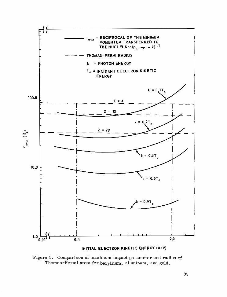
To obtain a calculable form for the initial wave function, one expands the wave function into spherical waves. The expansion of $. in spherical
waves, normalized in the energy scale, can be shown [ 171 to have the form 1
37
.
where
and s are constants, the values of which are determined from the
asymptotic form of the radial functions. In the Coulomb case, one finds that the difference between the Coulomb phase shift and that of the plane wave
is given by 6 ' and s = e (Appendix B) . For z,b one may write
K
i 6 ' K
K K i'
This can be simplified by taking the direction of propagation of the incident electron along the axis of quantization; say, the z axis. One first writes the spherical harmonic as
and from the recurrence relations for P one has [ 181 L Y
P; + (x) + PLM (x) + (Q+M) (1-M+l) Pa 2M M-I
( x ) = ( ) Y
( i-x2)1/2
where x = cos 8 . For propagation along the axis of quantization,
e = 0, x = I, and the recurrence relation becomes 0
0
38

PQM+I ( 1 ) + 2M PI ( I) + (Q+M) (4 "+I) PQ M M-I
(I)= 0 . ( 1-1)
The first and las t terms are f ini te but the second term becomes infinite as
x - I unless M = 0, PIM (I) = 0, o r both. That is, either Y = 0 o r
M = 0 . One must choose M = 0 (1.1 = m) ; otherwise, the wave function would Q
28 + I vanish. Now [ 191 , YQo ( e , 0) = ( 4n ) P (cos e ) ; and since P (I) =I , Q
After substitution and simplification, this expansion becomes
Expansion " of the Electromagnetic " Wave
The electFmagnetic wave denoted by the vector potential of the radiation field, A- in equation ( 18) , can be written as a linear combination
of waves that are circularly polarized [ I91 . ,,One first assumes that the wave is propagating along the z axis. Thus -if= k ] - i f 1 and one may write
k
( 19-a)
where, by definition, a = + I for a left-hand circularly polarized photon and
a = - I for a right-hand circularly polarized photon. P
P
39

Following the method used by Rose [ 191 , the electromagnetic wave denoted by A’ in equation ( 19-a) is expanded a s follows. For a plane wave
propagating along the vector k one writes the vector potential as P *
( 19-b)
where N is a normalization factor to be determined and E is the polarization vector for the photon; i. e. , a unit vector perpendicular to the propagation vector k and pointing in the direction of the electric field vector.
A
One then writes
with P = +I ( -1) for right (left) circular polarization by definition.
If the z axis is chosen to correspond to k, then l = e e2 = e 4 A A A A
A A A A X, Y Y
E,, = e where e e and e are the unit vectors along the x, y, and
z axes. The vector E may then be written in terms of the spherical basis vectors [ 191 where the vector B in the Cartesian basis can be transformed to the spherical basis, 5, by 5 = v where
Z, x, J , Z
“-L
-
o r
A
B = - I ( B x - i B ) . - G Y
40

Therefore one writes E in terms of the spherical basis A
h A E = -P 5, y
where 5, are the spherical basis vectors
A plane wave may be expanded by using the well known Rayleigh expansion; for an example, see Reference 19.
where j ( k r) are the spherical Bessel functions that are defined in terms
of the regular Bessel functions as Q
From the spherical harmonic addition theorem,
one may express the plane wave as
41

However, P (cos 0 ) = Q
; then, after substitution, one
has
co i k z = (47r)I/2 (-i) Q (2Q+1)1/2 jQ ( k r ) YQo ( r ) . e
A
Q =O
Therefore,
A' = - P 5, N 2 (-i) [ 47r( 2Q+1)]1/2 YQo ( r ) jQ ( k r ) . A Q A
P Q
The normalization factor, N, will next be determined to complete the expansion.
One first writes the vector potential representing a classical plane wave in t e r m s of time and position; i. e . ,
++ A ( x , t) = N n e
A i(E * X - w t)
where N is the normalization factor and n is the direction of propagation. This may be written as
A
A ' = N n [cos (E. % - u t ) ] .
Following the method presented by Feynman [ 121, AR is -
normalized to give unit probability per cubic centimeter of finding the photon. The average energy density is a w .
42

Prom Maxwell's equations, the electric field is
NOW 1 1 3 1 = 151 fo r a plane wave. Thus, one may write the average energy density as
-L
o r
since
@)AV 8nc%
However, = f i w ; then, , and in dimensionless units
Thus,
-L I/' A
A R ~ ~ ~ = (:) n [cos ( k * x - u t ) ]
o r
43

By taking the minus exponent, since one is considering the emission of a photon, and noting that w - k , in our system of units one has
where. E is the polarization vector. (See equations ( 19-a) and ( 19-b) . ) A
Finally, using equation (20) and the above normalization factor, the expansion for an electromagnetic wave propagating along the z axis is
4 A 1/2 A p = - P 5, (%) C ( -i) P [ 47r( 28 YPo ( r ) ja ( k r ) . A
Q
Next one defines the "vectorial spherical harmonic" as [ 191
m'-v A
v yP 5 - V
However,
has the inverse expansion
This implies that it is possible to write equation (21 ) a s
where h is the parity operator, h = P , P 5 I .
44

I
The expanded vector potential may now be written
%? = - P (~)i'z(h)i/z (-1) (21+i) i /2jI ( k r ) C o p ThIP 1 I l h
1,
To obtain a photon propagating along an arbitrary direction, one utilizes the rotation operator [ 191 , which has the property
The vector potential for a plane electromagnetic wave propagating along an arbitrary direction may then be written
From equation ( 18) , it is noted that
since L- = a p Kp . k P=*i
Since the purpose of this section is to derive the bremsstrahlung cross section differential in photon energy, the angular or polarization details of the scat tered e lectron are not of interest. Therefore, one may
45

express the final electron wave function a s
If an investigation of the angular distribution of the scattered electron were within the scope of this paper, one would expand I) in spherical waves.
These waves would behave asymptotically a s plane waves plus convergent spherical waves [ 111 with an expansion of the form
f
46

Equation (24) will next be integrated over the angles of the volume element. The square of the absolute value of the result will then be put in
the form lM . I = M 'f: Mfi . This expression will then be used to obtain f l f l the desired differential cross section.
The integral in equation (24) may be written as
0 1 since k * p
V
where - _a and b are any two matrices. Thus, -
One also defines the radial integrals a s
00
K( K ' K ) J jl ( k r ) g K T f K d r 0
m
Y
47

then,
The quantity in square brackets in equation (26) may be expanded as follows :
Now ,
From Reference 19, one has the expression
then,
V d-F $ & e v ) m a
= 2(-1) 6 m, a+v 2 a+v,-v . -
Therefore,
48

Now the integral over the angles can be evaluated by using:
then,
B B 8 1 8 8 ' K K ' ' K K '
x coo C m'-m+a! , p-a!
Thus equation (26 ) becomes
1 . 1 . P Q 8 P B B x c C C - K K ' -K K '
pf-my m p-a!, a! m,m+a! ' 0 0 m'-m+a! &-a!
Note that the only difference between the angular portion of 1, and I2 is the changing of K' t o -K ' and -K to K ; then,
49

Now, define
I +i I 3 j i d x i ( 2 1 COm K K K K
e [I1 - I21 K
or
I I I I 1 I K -K' K -K' C m,m+a '00 m'-m+cr ,p-a
Therefore, the matrix element, equation (24) , can be written as
( 32-a)
x p c ~ ~ m ' P k k ' I h D h ( c p 0 0 ) A ( h L K ' p f m a ) ,
50

( 32-b)
These matrix elements will now be used to find an expression for the differential cross section for bremsstrahlung production.
2 . THE DIFFERENTIAL CROSS SECTION
Recall from equation (7-b) that the differential cross section is given bY
The density of final states (equation 6) included in equation (33-a) is
Pf = (k) 6 Epk ' .
51
I

However, one assumes, for present purposes, that the photon is observed and the scattered electron is not observed. Therefore, since the Coulomb wave functions have been normalized in the energy scale, one writes the density of f inal s ta tes as (s ince p = 1 ) : f e'
and equation (33-a) becomes
o r
(33-b)
The matrix elements, M ( P, m,Kf,pl) , included in equation (32) a r e related to the matrix elements of equation ( 18) by the expression
Therefore, the differential cross section is given by [ ii]
where
E -2 0 +
dC&p = (2n) - M ( P1mK',ul) M( PmK'p') k2 dk d( cos e o ) d cp . rnK'I-1' 0
(35)
52

Using equation ( 3 2 ) for M (P'mK'p') M(PmK'p') and since the +
azimuthal angle of the photon is not of interest here, one writes
To perform the integration over the angle, the integration over the rotation operators is first considered; i. e . ,
Since the rotation operators are independent of q one may immediately
write . 0'
However,
Then,
I = 2n ('I) pt-m-P'
Dhl -p'+m, - P I Dh2 pl-rn, P
53

Now, since
and -p'+m+p'-m = O , the integral becomes
then,
one writes
(The fact that ( -i) = i has been used.) P' -P
The spherical harmonic can be written a s
54

where
are the associated Legendre functions. Thus,
I =27r c ( 4 ) p' -m-P' h2 j & 1 2 j
-,uf+m,p'-m j
-Ply P
The differential cross section, equation (36) , may then be written (since a = e2 in nuclear dimensionless units)
For unpolarized photons, equation (34) reduces to do ' = 2doi, . (The factor 2 has been included in the density of final states. ) Using equation (40) for do;, , one obtains the cross section for unpolarized photons
55
"""11"111.11111111.11.111 111 I111

This may be simplified by considering the orthogonality relation for the C-coefficients
Therefore, equation (41) becomes
The purpose of this report is to obtain the bremsstrahlung cross sec- tion differential in photon energy. Therefore, one integrates over the photon angle , . Note that the only angular dependence comes from the
associated Legendre function; one thus considers the integral
56

The only value of j
One then has
that contributes to the summation is, therefore, j = 0 . the bremsstrahlung cross section differential in photon
energy, for unpolarized incident electrons, and without regard to the scattered electrons or polarization of the emitted photon
where A" ( h l , l i , ~ ' , p'm) A ( A2,12, K ' , p'm) is given by equation (31) .
SECTION 1 1 1 . CROSS SECTION RESULTS
A computer program was developed by the author to calculate the Bethe-Heitler cross sections for any desired incident electron kinetic energy, a complete spectrum of photon energies, and the scattering media of interest. Results were initially obtained for incident energies from 0. I t o 2 . 0 MeV for aluminum, copper, tin, and gold. These materials were chosen s o that available experimental data could be utilized for comparison purposes and so that a wide range of atomic numbers would be used in the calculations. The results of these calculations are shown in Figures 6 through 9.
57

Z = y. 13
0.05 0.10 0.15 0.m
PHOTON ENERGY (MeV)
Figure 6 . Bremsstrahlung cross sections differential in photon energy for 0 .2 MeV electrons incident on aluminum, copper, tin, and gold.
58

- BETHE-HEITLER " - - PARTIAL WAVE
0 EXPERIMENTAL
0 0.1 0.2 0.3 0.4 0.5
PHOTON ENERGY (MeV)
Figure 7. Bremsstrahlung cross sections differential in photon energy for 0 .5 MeV electrons incident on aluminum, copper, tin, and gold.
59
I

BETHE-HEITLER -- -- PARTIAL WAVE 0 EXPERIMENTAL
1
0 0.2 0.4 0.6
PHOTON ENERGY (MeV)
Z = -13
I
0.8 1
1 .o
Figure 8. Bremsstrahlung cross sections differential in photon energy for I. 0 MeV electrons incident on aluminum, copper, tin, and gold.
60

0
BETHE-HEITLER
0 EXPERIMENTAL
0
Z = B
I I I I
0.4 0.8 1.2 1.6
PHOTON ENERGY (MeV)
Figure 9. Bremsstrahlung cross sections differential in photon energy for I. 7 MeV electrons incident on aluminum, copper, tin, and gold.
61

The experimental data for 0.2, i. 0, i. 7, and 2 . 5 MeV were obtained from Dance, et al . [ 71 while the data for 0 .5 MeV were obtained from Motz [ 61. It is noted that the experimental results of Motz give, in general, a higher value for the differential cross sections than the results of Dance, et al . , who attribute this difference between the two experiments to the presence of background in the experiment of the former. Since experimental data between 0 .2 and i. 0 MeV were required for comparison purposes, the author had t o use the 0 .5 MeV data from Motz as the only available data in this range.
The computer program first written by Zerby and Brysk [ i l l and expanded, reprogrammed, and improved by the Space Sciences Laboratory of NASA's Marshall Space Flight Center was used to calculate the bremsstrahlung cross sections using Coulomb wave functions. These results a r e a l so included for gold and aluminum.
It is noted from Figure 6 that for low incident electron kinetic energies the deviation of the Bethe-Heitler theory from the experimental results is appreciable. This deviation increases markedly for higher atomic numbers, as expected. In fact, it can be noted from Figure 6 that the theoretical ( Bethe-Heitler) cross section for gold is actually below the experimental resul ts for t in as the high frequency limit is approached. However, the Bethe- Heitler results improve when compared with experiment a s the incident electron kinetic energy increases, as expected.
The broken lines in Figures 6 through 8 indicate the differential cross sections that were calculated by using the correct Coulomb wave functions and the partial wave expansions. Note the very good agrement, in this energy range, between the experimental results of Dance, et a l . and the theoretical calculations.
Table I illustrates the importance of including the Coulomb effects for the energies that are considered here, Table I iists the relative error of the Bethe-Heitler theory because of the exclusion of Coulomb effects, assuming that the partial wave expansion approach results in the correct differential. cross section.
From the discussion in Section 11. C, subsection entitled Screening Effects by the Atomic Electrons, one can see that the small deviation of the Bethe-,Heitler theory above the experimental values at the low frequency end of the photon spectrum (Figs. 6 through 8) is a result of the exclusion of screening in making the calculations. In addition, note that the differential
62

z=79
- .
Z=13
TABLE i. THE APPROXIMATE RELATIVE ERROR O F THE BETHE-HEITLER THEORY WHEN COMPARED TO THE
PARTIAL WAVE RESULTS
q 0.2
0.5
I. 0
0.2
0.5
0.2
0.05
"
"
0.02
"
Relative Error
0.4
0.26
0.23
0.18
0.04
0.01
0.6
0.48
0.41
0.37
0.16
0.12
0.8
0.65
0.61
0.53
0.29
0.16
0.9
0.76
0.75
0.62
0.54
0.43
cross sections calculated by using the unscreened partial wave approach are also too large at the low frequency end of the spectrum. The much larger deviations of the Bethe-Heitler theory at the high end of the spectrum are almost entirely a result of Coulomb effects. This is shown schematically in Figure 10 where the differential cross section is plotted as a function of the ratio of the photon energy (k) to the incident electron kinetic energy (T ) .
0
SECTION IV. COULOMB CORRECTION FACTOR
A. Extension of the E lwer t Factor
The general approach used to obtain a correction to the Bethe-Heitler theory was to first calculate the cross sections, differential with respect to photon energy, using both the Born approximation and the partial wave expansion approach. Next , it was assumed that
63

PRlMARl LY COULOMB EFFECTS
“CORRECT” CROSS - . ,/ SECTION PRIMARILY SCREENING
\ \
\
\
B-H CROSS SECTION
0 0.2 0.4 0.6 0.8 1 .o
k/To
Figure 10. Schematic representation of screening and Coulomb regions.
where
is the differential cross section using the partial wave
A expansions ;
( 3 is the differential cross section obtained from the Born B approximation;
64

po = po/Eo , p = p/E as previously defined;
Z is the atomic number of the scattering medium;
and f ( p , po, Z) is the correction factor to be derived.
That is, it was initially assumed that the correction factor would be a function of the speed of both the incident and scattered electrons and the atomic number of the scattering material. The correction factor may then be written
To get an indication of the analytic form of this factor, the ratio of the cross sections was first computed and plotted a s a function of the ratio of the photon energy ( k ) and the incident electron kinetic energy ( T ) , a s shown in
Figure 11. From the resulting curve, it was first noted that the factor was similar to the Elwert factor in form (Fig. A-i(b) of Appendix A ) . There- fore, as an initial approach, it was assumed that the factor has the form
0
and determined the function, g( Z ) . Using multiple regression techniques, based upon a least squares
criterion, values of g( Z) were obtained using gold and aluminum as the scattering media. The most accurate function, assuming that t he form given by equation (46) is correct , is shown in Figure 12. The solid curves are the actual correction factors obtained from equation (45) while the broken line curves are from the regression equations. It was noted that the results are not very accurate; therefore, this analytic form for the factor was abandoned. It is of interest to note in passing, however, that, at an incident electron energy of 0.2 MeV, the results of the regression equation are almost identical to those of the Elwert factor.

5.0
4.0
3.0
f
2.0
1 .o
0
To = 0.2
I 1 1 1
0.2 0.4 0.6 0.8 1 .o k/T
Figure 11. The ratio of the differential cross sections calculated by the partial wave method to the Bethe-Heitler theory.
B. Al ternat ive Forms
From Figure 11, one can see that the curve has a value of 1. 0 a t k/T = 0 and has the general shape of a hyperbolic cosine function. Since
0
a cosh (x/a) = a/2 [exp(x/a) + exp( -x/a)] ,
66

5.0
4.0
3 .O
f
2.0
1 .o
ACTUAL - - - - COMPUTED
0 0.2 0.4 0.6 0.8 1 .o k/T,
Figure 12. Extension of the Elwert factor to higher energies for incident electron energies of 0 . 2 and 0 . 5 MeV incident on gold.
it was assumed that the correction has the analytic form
where y = k/T and g(p,, Z ) is an unknown function to be determined. 0
67

A curve f i t for f in terms of g(p , Z) was f i rs t obtained. This 0
resulted in different values of g for a given atomic number and specified value of p . The resul ts are shown in Figure 13, where the regression
0
curve is compared with the actual curve.
Figure 13. Comparison of calculated to actual correction factor.
The second step was to obtain the analytic form of g (p Z) . It 0)
can be seen from Figures 6 through 9 that the magnitude of the correction should increase with Z and decrease with increasing p . Therefore g
was plotted versus the parameter a = p o / Z since the exponents in 0
68

equation (47) are defined as y/g . Using standard regression techniques [ 201, the following function was obtained:
g(p , Z) = 0.394 + 9.47 (po/Z) . 0
Slightly more accurate functions were obtained but these had more complicated forms, Therefore, since the linear relationship gave relatively accurate results, it was used in these calculations.
The final form
f = - 1 exp I 2
of our correction factor was found to be
where
g = 0.394 + 9.47 (po/Z) . This can be written
= ‘Osh 1 ( 0.39%Z-+-9.47 p Z
0
(48-b)
C. Comparisons With Exper imental Cross Sect ions
The corrected cross sections were next calculated, using equation (48-a) in conjunction with equation (44), to make a comparison with the experimental cross sections. The results of these calculations are shown in Figures 14 through 16.
An inspection of Figures 14 through 16 indicates that the corrected Born approximation gives relatively good results for the energy range of primary interest. However, it may be noted from the 2.5-MeV curve in Figures 14 and 15 that the correction factor does not accurately predict the transition of the Born approximation from below to above the experimental results. This occurs between I . 7 and 2.5 MeV and was discussed in Section I. The failure is particularly apparent for high-Z materials. It is therefore concluded that the uncorrected Born approximation gives more accurate theoretical results in the energy range above, say, 2 . 0 MeV.
69

10”
10 -2 1
10 -22
31%
10 -23
10 -24
k BETHE-HElTbER
I I 1 I
0 0.2 0.4 0.6 0.8
k/Ta 1 .o
Figure 14. Comparison of Bethe-Heitler and corrected differential cross sections for 0.2, I. 0, I. 7, and 2.5 MeV electrons incident on gold.
70

1 To = 0.2
- BETHE-HEITLER - --- CORRECTED 6-H 0 EXPERIMENT
I I I I I
0 0.2 0.4 0.6 0.8 1 .o k/T,
Figure 15. Comparison of Bethe-Heitler and corrected differential cross sections for 0 . 2 , I. 0, I. 7, and 2.5 MeV electrons incident on t in.
71

,..-.".... CORRECTED B-H
EXPERIMENT
t
I I I I 1
0 0.2 0.4 0.6 0.8
k/To
1.0
Figure 16. Comparison of Bethe-Heitler and corrected differential cross sections for 0.2, I. 0, I. 7, and 2 . 5 MeV electrons incident on aluminum.
72

It may be noted from Figures 14 through 16 that the corrected differential cross sections are closer to the experimental results for lower
. energies. This is most likely because of the fact that the partial wave data used in the derivation of the correction factor were limited to lower energies.
SECT I ON V. CONCLUSIONS
The bremsstrahlung cross section has been calculated using both a partial wave expansion that includes correct Coulomb wave functions and the Born approximation. It was found that the former approach gives better agreement with experiment in the 0.1- t o I. 0-MeV energy range. In fact, the Born approximation differs appreciably from the experimental data, especially for high atomic numbers and lower energies. For example, the greatest deviation was found to be about 75 percent for 0.2-MeV electrons incident on gold if the photon received 90 percent of the incident electron kinetic energy. On the other hand, at 2.5 MeV the Born approximation gave relatively good agreement with experimental results.
Screening effects due to the atomic electrons were found to be insignificant in the energy range of interest , except for photons with a low percentage of the incident electron kinetic energy. Therefore these effects were not included in these calculations.
A correction factor to the Born approximation was derived by comparing the two theoretical approaches. This factor is a function of the photon share of the incident electron energy (k/T ) , the velocity of the
incident electron ( P /E ) , and the atomic number of the scattering media. 0
0 0
The corrected Born approximation was then calculated for incident electron energies from 0.2 to 2.5 MeV, and for a range of atomic numbers.
It was found that the corrected cross sections gave relatively accurate results at the lower portion of the energy region under investigation; while, at energies above this range, e. g. , a t 2 .5 MeV, the uncorrected cross sections were more accurate.
The correction factor failed to give accurate results after the Born approximation passed through the "transition region. This was most likely a result of the limitation of the data available from the partial wave method.
73

A t the present time, this method has an upper limit of around I. 0 MeV. However, should improvements be made in the computer program, it may be possible to obtain a correction factor that is more accurate in the higher energy range than the present case seems to indicate.
George C. Marshall Space Flight Center National Aeronautics and Space Administration
Marshall Space Flight Center, Alabama, A p r i l 27, 1970 124-09-11-14
74

APPENDIX A
ELWERT COULOMB CORRECTION FACTOR FOR LOW ENERGIES
To cor rec t for the Coulomb effects not included in the born approximation, Elwert [ 91 developed a correction factor valid up to an energy on the order of 0 .1 MeV. This factor was derived by applying the techniques of mathematical analysis to a comparison between the non- relativistic Born approximation and the exact Sommerfeld results. It is therefore a semi-empirical factor limited to electrons with velocities in the nonrelativistic range. The Elwert factor may be written as
The corrected cross section is then obtained by
( atomic
- -
Figure A - I ( a) shows the magnitude of this factor for a range of numbers, photon energies, and incident electron kinetic energy.
Figure A-2 illustrates the effect of the Elwert factor on the Bethe- Heitler differential cross sections and makes a comparison with the experi- mental results obtained from Reference 7.
Note that f - I a s k - 0. This is t rue s ince f approaches 1 E E asymptotically as p - P o ; i.e. , a s k - 0.
The maximum energy that can be radiated in a bremsstrahlung collision is limited to the incident kinetic energy,
known as the "high frequency (short wavelength) limit. A s this limit is approached, the Bethe-Heitler theory breaks down since, contrary to experimental data, it predicts a vanishing cross section [ 51. The Elwert factor does not correct for this . To illustrate this, one first notes that the Elwert factor [ 51 is valid only if
(hv )max o = T . This is
75

0 2
/ \ 30 - k = 0.7T,
(Z = 79) \
\ 20 -
X
7 n
I W
Y
Y
0
8
k = 0.5T.
INCIDENT ELECTRON KINETIC ENERGY (MeV)
Figure A - i ( a ) . Elwert Coulomb correction factor - effect of atomic number and photon energy on magnitude of correction.
I HIGH FREQUENCY LIMIT 4 60
0 40 s n X
c I
Y W
v 20
0 20 40 60 80 100
k/To (x)
Figure A-i(b) . Elwert factor for 0 . 3 MeV incident electrons a s a function of photon fractional energy.
76

0
BETHE-HEITLER "" BETHE-HEITLER CORRECTED
BY ELWERT FACTOR
SECTIONS EXPERIMENTAL CROSS
I - I 1 I I
0.02 0.06 0.10 0.14 0.16
PHOTON ENERGY (MeV)
Figure A-2. Effect of Elwert factor on bremsstrahlung cross sections for 0 . 2 MeV electrons incident on aluminum, copper, and gold.
77

(Z/137) (p-' - Po ) << I . -1
Since p = ( E2 - and p = ( E t - I) , one may wri te 0
then our restriction becomes
-1/2 - E 0 ( E t - I .
Now E = k + E by conservation of energy; and, since Eo = To + I , 0
then E = T + i - k. A s the high frequency limit is approached, k - T
then E - i and one has in the 0 0 ,
lim k - T Z/137 [E( 1 - 1) - Eo(Eo
-1/2 - I) -I"]<< I . 0 '
E - 1
Thus, the second term approaches infinity and the Elwert factor is not valid at the high frequency limit ( Fig. A - I ( b) ) .
It can be concluded from the data presented and the above argument that the Elwert factor is valid for lower energies and increases as the high frequency limit is approached or the atomic number of the scattering medium increases. Furthermore, the factor cannot be used at the high frequency limit, since it increases without bound at that point.
78

APPENDIX B
NORMALIZATION OF THE RADIAL WAVE FUNCTIONS
The radial functions for the continuum states are normalized on the energy scale. This requires that [ 171
First, consider the asymptotic form of the radial functions. A s r - w
The asymptotic form is also given by letting r - 03 in equation ( C - i i ) , Appendix C; i.e.
r g - ( E+I) 1'2 N r (2y+ i ) ( 2 p r ) +iy) exp( i p r +iq) r ( y +i+iy)
Now [17],
y+iy - exp[ -i ARG I7 ( y +iy)] ( y +i+iy) I r ( y + i y ) I
- 9
79
I

I
and since m-
and
the first term in square brackets of equation (B-2a) can then be written as
-Y 7r
7r ip r - - 2 y
(2pr) exp[ i( -ARG I7 (y+iy)+y In 2pr - 2 y+q)] e I r (y+iy) I
Define 6 = y In (2pr) - ARG r (y+iy)+q - 2 y ; then, 7-r
r f - i (E- i )1 /2 N r ( 2 y + i ) ( 2 ~ r ) ~ ( 2 ~ r ) ~ (eXP[ i ( P r -7 7r Y +6) ]
- exp [ -i (Pr - 2 Y + 6)] } , 7r
o r - - 7 , 7-r
2( E-1)1/2 N I? (2y+I) e I r ( y + i y ) I
2 y rf - s i n ( p r + 6 ) ( B -2b)
A comparison of equations (B-I) and (B-2b) indicates that these equations will be equal a s r - 00 , if
TY
Now use the rule for normalization of the eigenfunctions of the continuous energy spectrum [ 211
80

00 P+A P 1 r 2 d r f p ( r ) fp , ( r ) dp' = 1 , 0 P-A P
The asymptotic form of f is given by equation (B-I) a s
f = A / r [ cos (p r + 6 ) ] .
Consider the second integral in equation (B-4)
'7' d;' 2 - cos( p ' r + 6 ) = - cos (p r + 6) s i n A p r Y r r
P-A P
where values on the order of i / p r and A p/p have been neglected. Substitution of this result into equation (B-4) gives, after replacing the oscillating function cos2( pr + 6 ) by its average value & ,
A 2 s i n A p r d r = i . 0
r
This integral can be found in any standard table of integrals; then,
This is the normalization factor on the energy scale.
If fE are eigenfunctions normalized on the energy scale, and f p
a r e eigenfunctions normalized on the momentum scale, they are relatedby [21]
4 2
fE =(%) fp *
81

Since E = 4p2 , then fE = p fp . Thus, on the energy scale, one - 1/2
1/2 has A = (5) . This value of A must be set equal to the value of A
found in equation (B-3) to determine N, the radial function normalization factor. Hence,
. ~~
2 N r ( 2 y + i ) e "
I r (y+iy) I
o r
Z e 2 E where y = - P
82

APPENDIX C
THE DIRAC EQUATION IN POLAR COORDINATES
The bremsstrahlung problem is described by a relativistic electron in a central field. The equation of motion for this particle is given by the Dirac equation using the Hamiltonian:
and
H $ = E$
where - $ and are the Dirac matrices defined below and - -
Since a central field has been assumed, the Dirac equation will be separated into polar coordinates using the method presented by Rose [ 191. (In this appendix, extensive use will be made of two books by M. E . Rose [ 17,191 .)
First one writes the gradient using the identity
where r is the position vector for the Dirac particle relative to the field source. Since L = -i r x V , where L is the orbital angular momentum
+ " +
83

operator, one has
For any two vectors A' and whose components commute with the - components of (r the 2 x 2 Pauli spin matrix, one has (c. - ( r - - g:?. g+iz* - ( ~ x .
1 0 0 0
0 1 0 0 I E t h e 4 x 4 unit matrix (," ~ ~ :) ' - -
For example,
, etc.
84

Note that
4 -4 "c
Consider p * A B , where A' and Ii' are any vectors whose components commute with th? components of _o . One has
"c
-
Now, since p3 = p3 , then -1
- - -
where the subscript 4 indicates a 4 x 4 matrix.
However,,
then,
- - Let A r and B L ; then, by using a vector identity
"
one has A B = 0 . + -
85

Thus,
\ O
4
4 - c 4 4 4 + - 4
Therefore, Q * r L = i g - r x L . Now, r Q! - I = g r , - - - - r =
+ " -L
where Q! is a 4 x 4 matrix and i g r x L = 9 c - L ; then +
=r - - r =
" a Also, since g * V = g - - - CY - r x L (from equation C-2), i - 4 4
- -r 8 r r - -
The Dirac equation can now be written as
Now, define the operator [ 191
86

o r
- NOW, (c+ ;/$' = J2 , the total angular momentum operator, with
eigenvalues j( j + I) . Define the eigenvalues of K t o be - K ; i. e. ,
or
2 Therefore, the eigenvalues of K2 are K' =( j + -$ K = *I, * Z , h3 , . . - o r j = I K I -- , K f 0 ; where, for the upper
spinor (equation C-5) 2
I = K if K > O
I = -K-I if K < 0 .
This could be written as I = j + - S( K ) , where S( K ) is the sign of
kappa; i.e., S ( K ) = K / I K I . I 2
To indicate the dependence of j and I on K , the eigenvalues of j by j K and I by lK in the upper spinor are replaced. For the lower spinor
(equation C-5) , define

where
for K > 0
for K < 0
That is,
The wave function for the Dirac equation is written as
U Q where 9 and - $ are the two-component, single-column matrices referred to as thz "upperiT and "lower" functions, respectively. The wave functions are proportional to the angular functions, 8 and i2 , respectively,
where the eigenvalue 1-1 is the z component of the total angular momentum. K P -KP
The angular functions may be written as a product of the orbital angular momentum function and the intrinsic spin function, coupled by the vector addition or Clebsch-Gordon coefficients:
where the two-component Pauli spinors are defined as rl - 2, 2
88

One expresses the wave function p a s "K
where f and g are the radial wave functions.
Substituting - $ into equation ( C - 3 ) one has, after noting that -
where the primes denote differentation with respect to r .
the Dirac equation becomes
89

From equation (C-4) ,
which implies that
since _K z,b = - K . Then
" - -
One next considers 0 and follows the proof given by Rose [ 171 -r KP
t o find the results of carrying out this operation. Now g is a pseudoscalar
operator s o that j 2 commutes with g . That is, for j - - r
- r 2 ,
since
( a Z y x) = iY, (IZY Y) = -ix, (SZ' ,ax) = i a , -Y
and (S , g ) = -i cr . Now, since o has odd parity, z -Y = X =r
r t
90

where a2 = I , since (T = 1 . The latter follows from the result
- (T A _a B = A B + i _o ( A x B) , which implies that
(T =;. r g . r = r - r + i g - (r x r) = l2 + i a (0 ) = I . Now take r along
the Z axis; then e = 0 . The spherical harmonic in the definition of S2 .
becomes
" "+ - 4 -
=r
- - - A - A A A - - A A
=r - - - - + A
W
Setting m = 0 will then give
- Q & j 8 & j Therefore , a( 21 C = 2p( 28 +I)+ c . There a r e K K
K O P K 01-1 four possible cases:
One finds, after substitution of these values and solving for a, that a = -1 for all four possibilities. Therefore,
and, by the same type of argument, one can show that
91

After one operates on the angular functions with the operators 4 4
( i + - o L ) and ur , one's set of equations becomes - - -
[(E-V-i) g + f l + f/r - K f / r ] fi = 0 K P
i[ (E-V+i) f - g' - g/ r - K g/r l fi -KP = 0 *
This implies that the expression in square brackets must equal zero; i. e . ,
(E-V-I) + f ' + f/r - K f/r = 0
(E-V+l) - g' - g/r - K g/ r = 0 .
For simplicity, one writes ui = r g and u2 = rf; then equation ( C - 6 ) becomes
dui = " K UI + (E+I-V) ~2
d r r
These are the radial equations of a Dirac particle in a central field. The boundary conditions required are that the resulting solutions must remain finite a s r - 0 and a s r - 03 .
The asymptotic forms of equation (C-7) a r e found by assuming that the potential tends to zero sufficiently fast for large r ( i . e . , V - 0 as r - 0 3 ) .
For large r, equation ( C - 7 ) becomes
9 - ( E + i ) u 2 = 0 d r
du3 + ( E - I ) u l = O . d r
92

The genera1.solutions for these equations are
ui = N(e-Ir + q ( E ) eAr)
and
where h = ( I -E ) , 2 1/2
N is the normalization factor, and
q( E) is found from the condition that the solutions remain finite a s r - 0.
Since E > I , let p = ( E2 - I)’/’ so that h = i p ; equation (C-8) then becomes
where p is the momentum of the particle and 6 is the phase shift that will depend upon the nature of the external field of the particle.
Following the method of Rose [ 171 , one lets V = -ze/r Z / r in equation ( C-7) ; i. e. ,
and
93

After the substitutions
and
x = 2 i p r (where $1 and @ 2 are functions of x) are made, one then has
and
i ZE dx x
After taking the complex conjugate of these equations, i. e.
and
one can see by inspection that the two sets of equations are equal i f $1:: = $2 . After eliminating 5b2 one has
+2" x d x * - [ $ . ( + + - - ) + + f ] $ , = O i Z E (C-9)
where y = [K' - Z 2 ] 'I2 .
94

1 Let M = x 2 @i to get equation (C-9) into the standard form of
-
Whittaker's equation
Equation (C-9) becomes
This equation has the regular solution at r = 0 :
where y = ZE/p and F (y + 1 + iy, 2y + i, x ) are the confluent hypergeometric functions [ 221
a a (a+ i ) x2 m a m m x + . . . = - - C m! F ( a , c , x ) = i + - x + C c(c+i) 2!
- m=O m
- 1
Now, M = x ; then
G l = x e F ( y + 1 + iy, 2y + i, x ) y -x/2
= N ( y + iy) eiq (2pr) e F ( y + i + iy, 2y + i, 2ipr)
- N ( y + i y ) e ir7 (2PIY @ (r) Y
y -ipr
where N is the normalization factor. Next, the phase of 7 is chosen such that G2 = @: ; this requires that [ 171
95

This equation can be evaluated by using Kummer's formula
and
xF(a + I, c + I, x) = C [F(a + I, cy x ) - F ( a , c , x ) ] .
One finds that
2iq K - iy/E e = - Y + i Y
(C-IO)
The radial wave functions may then be written
rf = i ( E - N(Xpr) '((y+iy) exp(-ipr + i q )
x F(y+l+iy, 2y+i, 2ipr) + complexconjugate} ,
where N is the normalization factor and q is the phase determined from equation ( C-IO) .
The solutions are normalized in the energy scale. If $E and $ E' are solutions corresponding to energies E and E', then one requires that
96

From Appendix B, equation (B-5), the normalization constant is
TV
Therefore, the radial wave functions for a particle in a Coulomb field normalized on the energy scale, and with energy corresponding to the continuous energy spectrum, are
(C- i2)
x ( y + iy) F(y + i + i y , 2y +. I, 2ipr) - C . C . }
97

REFERENCES
I. Sommerfeld, A. : Atombau and Spektrallinien 11. Braunschweig, 1939.
2. Bethe, H. A. ; and Heitler, W. : Proc. Roy. SOC. , vol. A146, London, 1934, p. 83.
3. Schiff, L. I. : Phys. Rev. , vol. 83, 1951, p. 252.
4. Bethe, H. A . ; and Maximon, L. C.: Phys. Rev., vol. 93, 1954, p. 768.
5. Koch, H. W. ; and Motz, J. W.: Rev. Mod. Phys. , vol. 31, 1959, p. 92.
6. Motz, J. W.: Phys. Rev. , vol. 100, 1955, p. 1560.
7. Dance, W. E . ; Rainwater, W. J.; and Rester, D. H.: Investigation of Electron Interaction in Matter. LTV report no. 0-71000/8R-2, February 1968. (To be published in Phys. Rev. ).
8. Starfelt, N. ; and Koch, H. W. : Phys. Rev., vol. 102, 1956, p. 1598.
9. Elwert, G.: Ann. Physik, vol. 34, 1939, p. 178.
10. Zerby, C. D. ; and Keller, F. L. : Nucl. Sci. and Eng., vol. 27, 1967, p. 190.
11. Brysk, H.; Zerby, C. D. ; and Penny, S. K.: Phys. Rev. , vol. 180, 1969, p. 104.
12. Feynman, R. P.: Quantum Electrodynamics, A Lecture Note and Reprint Volume. W. A . Benjamin, Inc., New York, 1955.
13. Schiff, L. I. : Quantum Mechanics. McGraw-Hill Book Company, Inc. , New York, 1955.
14. Heitler, W. : The Quantum Theory of Radiation. Oxford University Press, London, 1954, 3rd ed.
15. Akhiezer, A. I. ; and Berestetskii, V. B. : Quantum Electrodynamics. Interscience Publishers, John Wiley and Sons, Inc. , New York, 1965.
98

REFERENCES (Concluded)
16. Bethe, H. A . : Proc. Cambridge Phil. SOC. , vol. 30, 1934, P. 524.
17. Rose, M. E. : Relativistic Electron Theory. John Wiley and Sons, Inc. , New York, 1961.
18. Abramowitz, M. ; and Stegun, I. A . : Handbook of Mathematical Functions With Formulas, Graphs, and Mathematical Tables. National Bureau of Standards, Washington, D. C. , 1964.
19. Rose, M. E. : Elementary Theory of Angular Momentum. John Wiley and Sons, Inc. , New York, 1955.
20. Hilderbrand, F. B. : Introduction to Numerical Analysis. .McGraw-Hill Book Company, Inc. , New York, 1956.
21. Bethe, H. A . ; and Salpeter, E. E. : Quantum Mechanics of One-and-Two Electron Atoms. Academic Press, Inc. , New York, 1957.
2 2 . Matthews, J. ; and Walker, R. L. : Mathematical kethods of Physics. W. A . Benjamin, Inc., New York, 1964.
NASA-L.angley, 1970 - 24 M436 99

NATIONAL AERONAUTICS AND SPACE ADMINISTRAT ION
WASHINGTON, D. C. 20546
OFFICIAL BUSINESS FIRST CLASS MAIL
'OSTAGE AND FEES PAID ~~ ~ . . ~ ~
0 6 U 001 49 51 3DS O2 * ;PACE ADMINISTRATION
A I R F O R C E WEAPONS L A B O R A T O R Y /WLOL/
rI0NAL AERONAUTICS AN
K I R T L A r V O A F B I NEW M E X I C O 87117
A T T E - LOU BOWMAN, CHIEFVTECH. L I H R A R Y
m~TMASTER: If Undeliverable (Section 158 Postal Manua l ) Do Not Recur,
"The aeronatltical and space nctivities of the United Stntes shall be condutted so as to contribzrte . . . to the expansion of huntan knowl- edge of phenomena in the ntvtosphere and space. The Adntinistration shall provide for the widest prncticable and appropriate dissemination of inforlnation concerning its nctitities and the resdts thereof."
-NATIONAL AERONAUTICS AND SPACE ACT OF 1958
NASA SCIENTIFIC AND TECHNICAL PUBLICATIONS
TECHNICAL REPORTS: Scientific and technical information considered important, complete, and a lasting contribution to existing knowledge.
TECHNICAL NOTES: Information less broad in scope but nevertheless of importance as a contribution to existing knowledge.
TECHNICAL MEMORANDUMS: Information receiving limited distribution because of preliminary data, security classifica- tion, or other reasons.
CONTRACTOR REPORTS: Scientific and technical information generated under a NASA contract or grant and considered an important contribution to existing knowledge.
TECHNICAL TRANSLATIONS: Information published in a' foreign language considered to merit NASA distribution in English.
SPECIAL PUBLICATIONS: Information derived from or of value to NASA activities. Publications include conference proceedings, monographs, data compilations, handbooks, sourcebooks, and special bibliographies.
TECHNOLOGY UTILIZATION PUBLICATIONS: Information on technology used by NASA that may be of particular interest in commercial and other non-aerospace applications. Publications include Tech Briefs, Technology Utilization Reports and Technology Surveys.
Details on the availability of these publications may be obtained from:
SCIENTIFIC AND TECHNICAL INFORMATION DIVISION
NATIONAL AERONAUTICS AND SPACE ADMINISTRATION Washington, D.C. PO546