To Hydrate or Chlorinate: A Regression Analysis of the

University of Central Florida University of Central Florida

STARS STARS

HIM 1990-2015

2015

To Hydrate or Chlorinate: A Regression Analysis of the Levels of To Hydrate or Chlorinate: A Regression Analysis of the Levels of

Chlorine in the Public Water Supply Chlorine in the Public Water Supply

Drew A. Doyle University of Central Florida

Part of the Statistics and Probability Commons

Find similar works at: https://stars.library.ucf.edu/honorstheses1990-2015

University of Central Florida Libraries http://library.ucf.edu

This Open Access is brought to you for free and open access by STARS. It has been accepted for inclusion in HIM

1990-2015 by an authorized administrator of STARS. For more information, please contact [email protected].

Recommended Citation Recommended Citation Doyle, Drew A., "To Hydrate or Chlorinate: A Regression Analysis of the Levels of Chlorine in the Public Water Supply" (2015). HIM 1990-2015. 1863. https://stars.library.ucf.edu/honorstheses1990-2015/1863

https://stars.library.ucf.edu/



https://stars.library.ucf.edu/honorstheses1990-2015

http://network.bepress.com/hgg/discipline/208?utm_source=stars.library.ucf.edu%2Fhonorstheses1990-2015%2F1863&utm_medium=PDF&utm_campaign=PDFCoverPages

https://stars.library.ucf.edu/honorstheses1990-2015

http://library.ucf.edu/

mailto:[email protected]

https://stars.library.ucf.edu/honorstheses1990-2015/1863?utm_source=stars.library.ucf.edu%2Fhonorstheses1990-2015%2F1863&utm_medium=PDF&utm_campaign=PDFCoverPages



TO HYDRATE OR CHLORINATE:

A REGRESSION ANALYSIS OF THE LEVELS OF CHLORINE

IN THE PUBLIC WATER SUPPLY

by

DREW A. DOYLE

A thesis submitted in partial fulfillment of the requirements

for the Honors in the Major Program in Statistics

in the College of Sciences

and in the Burnett Honors College

at the University of Central Florida

Orlando, Florida

Fall Term 2015

Thesis Chair: Dr. Liqiang Ni

ii

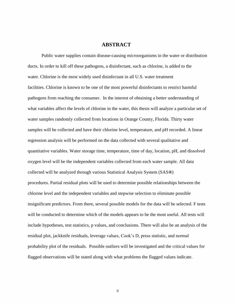
ABSTRACT

Public water supplies contain disease-causing microorganisms in the water or distribution

ducts. In order to kill off these pathogens, a disinfectant, such as chlorine, is added to the

water. Chlorine is the most widely used disinfectant in all U.S. water treatment

facilities. Chlorine is known to be one of the most powerful disinfectants to restrict harmful

pathogens from reaching the consumer. In the interest of obtaining a better understanding of

what variables affect the levels of chlorine in the water, this thesis will analyze a particular set of

water samples randomly collected from locations in Orange County, Florida. Thirty water

samples will be collected and have their chlorine level, temperature, and pH recorded. A linear

regression analysis will be performed on the data collected with several qualitative and

quantitative variables. Water storage time, temperature, time of day, location, pH, and dissolved

oxygen level will be the independent variables collected from each water sample. All data

collected will be analyzed through various Statistical Analysis System (SAS®)

procedures. Partial residual plots will be used to determine possible relationships between the

chlorine level and the independent variables and stepwise selection to eliminate possible

insignificant predictors. From there, several possible models for the data will be selected. F tests

will be conducted to determine which of the models appears to be the most useful. All tests will

include hypotheses, test statistics, p values, and conclusions. There will also be an analysis of the

residual plot, jackknife residuals, leverage values, Cook’s D, press statistic, and normal

probability plot of the residuals. Possible outliers will be investigated and the critical values for

flagged observations will be stated along with what problems the flagged values indicate.

iii

ACKNOWLEDGEMENTS

I would like to thank Dr. Liqiang Ni, Dr. Hsin-Hsiung Huang, and Dr. Andrew Randall for all of

their help and support throughout this project. Without them this project would not have been

possible. I would also like to thank everyone else who has supported me during this project. This

has truly been a tough, but rewarding experience.

iv

TABLE OF CONTENTS

INTRODUCTION......................................................................................................................... 1

METHODOLOGY ....................................................................................................................... 5

GETTING THE DATA INTO SAS............................................................................................. 9

VARIABLES ............................................................................................................................... 11

FINDING THE BEST MODEL ................................................................................................ 18

ANALYZING THE CHOSEN MODEL ................................................................................... 22

F Test ........................................................................................................................................ 22

Prediction Quality ................................................................................................................... 23

Parameter Estimates ............................................................................................................... 24

PRESS Statistic ....................................................................................................................... 24

Outliers..................................................................................................................................... 25

Variance Inflation Factor ....................................................................................................... 27

Pearson Correlation Coefficients........................................................................................... 27

Residual Plots .......................................................................................................................... 29

Normality ................................................................................................................................. 30

CONCLUSION ........................................................................................................................... 32

FUTURE RESEARCH ............................................................................................................... 33

APPENDIX A: DATA ................................................................................................................ 35

APPENDIX B: SAS CODE ........................................................................................................ 37

APPENDIX C: SAS OUTPUT ................................................................................................... 40

REFERENCES ............................................................................................................................ 75

v

LIST OF TABLES

Table 1: Summary of Forward Selection .................................................................................. 19

Table 2: Summary of Backward Elimination .......................................................................... 20

Table 3: Summary of Stepwise Selection .................................................................................. 20

Table 4: F Test for Chosen Model ............................................................................................. 23

Table 5: Prediction Quality of Chosen Model .......................................................................... 23

Table 6: Parameter Estimates for Chosen Model .................................................................... 24

Table 7: PRESS Statistic of Chosen Model .............................................................................. 24

Table 8: Check for Outliers ....................................................................................................... 25

Table 9: Variance Inflation Factor ............................................................................................ 27

Table 10: Pearson Correlation Coefficients ............................................................................. 28

Table 11: Tests for Normalitys .................................................................................................. 30

vi

LIST OF FIGURES

Figure 1: Chlorine Breakdown .................................................................................................... 2

Figure 2: Water Supply Flow Diagram ...................................................................................... 3

Figure 3: Map of Orange County Water Service Areas ............................................................ 6

Figure 4: Scatter Plot of Location and Total Chlorine ........................................................... 11

Figure 5: Scatter Plot of Time of Day and Total Chlorine ...................................................... 12

Figure 6: Scatter Plot of Temperature of the Water and Total Chlorine .............................. 13

Figure 7: Scatter Plot of Sample Storage Time and Total Chlorine ...................................... 14

Figure 8: Scatter Plot of pH and Total Chlorine ..................................................................... 15

Figure 9: Scatter Plot of Dissolved Oxygen and Total Chlorine ............................................ 16

Figure 10: Histogram of Total Chlorine Levels ....................................................................... 17

Figure 11: Residual Plots............................................................................................................ 29

Figure 12: Distribution and Probability Plot of the Residuals ............................................... 31

1

INTRODUCTION

Public water supplies contain disease-causing microorganisms in the water or transport

ducts. In order to kill off these pathogens, a disinfectant, such as chlorine, is added to the water.

“Disinfection is the last treatment stage of a Drinking Water Treatment Plant (DWTP) and is

carried out to maintain a residual concentration of disinfectant in the water distribution system.”

(Sorlini) The introduction of water disinfectants in the 20th

century was considered to be one of

the greatest progressions in health decreasing both typhoid and cholera outbreaks (Lyon).

Chlorine is the most widely used disinfectant in all U.S. water treatment facilities. “Chlorine is

still an indispensable disinfection agent because of the assurance of a high microbiological

stability of water in the distribution subsystem…” (Zimoch). Chlorine is used as a disinfectant

for a variety of reasons. “As a chemical disinfectant, chlorine has been applied to treat potable

water widely because it is relatively cheap and effective.” (Wang) Chlorine is known to be one

of the most powerful disinfectants to restrict harmful pathogens from reaching the consumer.

“While disinfectants have provided a novel method as a means to clean water, their usage leads

to the formation of unwanted drinking water disinfection by-products (DBPs)” (Ali) These

DBP’s can form from the interaction between the disinfectant and the organic materials naturally

within the water.

By trying to eliminate harmful pathogens from our water supply, we are creating a new

threat that our bodies must defend against. “Several epidemiological studies have shown that

consumption or exposure to water above the maximum containment levels of DBPs in water

have been associated with problems of liver, kidney, the central nervous system and increased

2

risks of bladder, and colorectal cancers.” (Ali) If someone has to choose, people are better off

drinking elevated DBPs than they are drinking inadequately disinfected water. This method of

cleansing the water is not perfect, but it is better than not disinfecting the water at all.

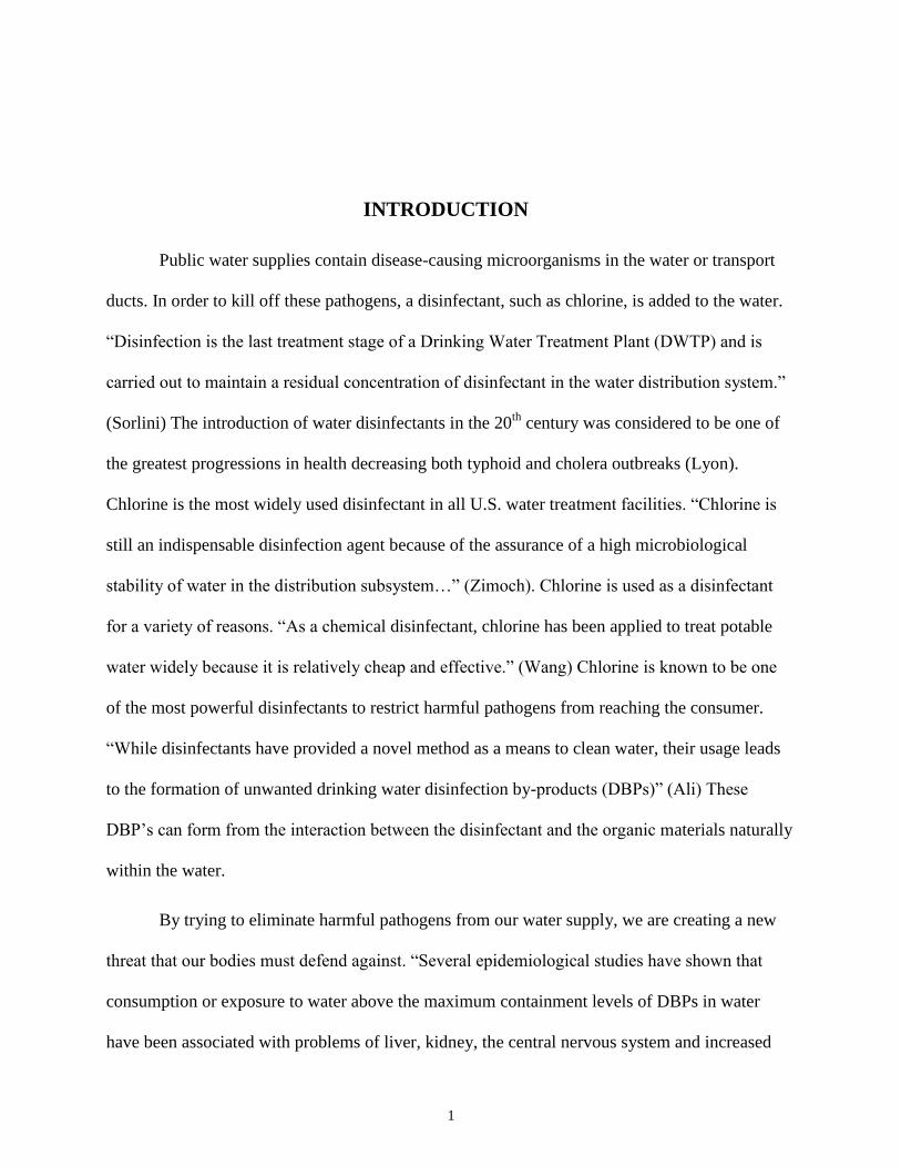
Figure 1: Chlorine Breakdown

This image above, provided by the Centers for Disease Control and Prevention,

summarizes what happens to chlorine when it is added to the water. When chlorine is added to

the water it is broken into Chlorine Demand and Total Chlorine. The Total Chlorine is separated

into two categories: Free Chlorine and Combined Chlorine. The Combined Chlorine is where the

DBP’s, such as ammonia, are formed when the chlorine reacts with the other compounds present

3

in the water. The Combined Chlorine is not as effective for disinfecting the water, unlike the

remaining Free Chlorine.

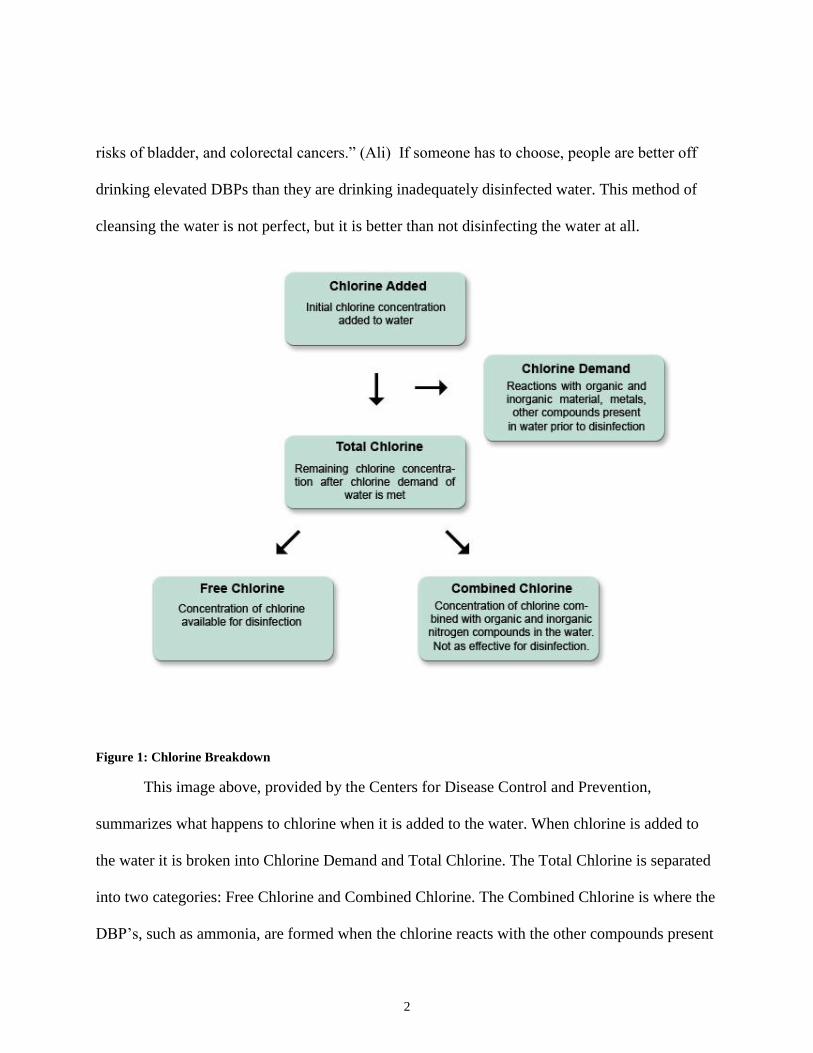
Figure 2: Water Supply Flow Diagram

From the water supply flow chart provided by Orange County, one can see that chlorine

is added to the water twice before it is released to the distribution system. Chlorine is added to

the water before it enters the storage tank and then once again right before it goes out to the

distribution system.

Several variables can affect the chlorine currently in the water, whether they increase or

decrease the amount of chlorine. Ideally a consumer would like to decrease the amount of

chlorine in their water before consuming or using it. “Chlorine decays in water because of its

4

reactions with inorganic and organic solutes that impose chlorine demands.” (Liu) The amount

of chlorine in the water will decrease as it reacts with the microorganisms present in the water.

“Chlorine loss in aged samples (samples left in open bottles) was greatest (approximately 40

mg/L free chlorine loss in 24 h) in low pH (approximately 2.5) and high chloride (Cl-)

concentrations (greater than 150 mg/L).” (Waters) As water is left to sit, the amount of chlorine

present should decrease. Chlorine levels should be lower when the pH level is more acidic.

5

METHODOLOGY

In the interest of obtaining a better understanding of what variables affect the levels of

chlorine in the water, this paper will analyze a particular set of water samples randomly collected

from locations in Orange County, Florida. Thirty water samples, ten samples from each of the

main three treatment plant service areas and each from a different location within the service

areas, will be collected and have their chlorine level, temperature, pH, and dissolved oxygen

level recorded. The chlorine levels will be read by a LaMotte Model DC1100 Colorimeter and

will output the amount of chlorine in parts per million (ppm). This colorimeter will read the total

chlorine of the sample, including both free and combined chlorine levels. The collected data

“tells us about how one or more factors might influence the variable of interest.” (Bowerman) In

this research the variable of interest is the chlorine level of the water for Orange County, FL.

6

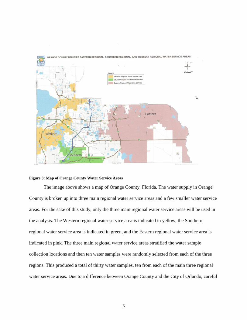
Figure 3: Map of Orange County Water Service Areas

The image above shows a map of Orange County, Florida. The water supply in Orange

County is broken up into three main regional water service areas and a few smaller water service

areas. For the sake of this study, only the three main regional water service areas will be used in

the analysis. The Western regional water service area is indicated in yellow, the Southern

regional water service area is indicated in green, and the Eastern regional water service area is

indicated in pink. The three main regional water service areas stratified the water sample

collection locations and then ten water samples were randomly selected from each of the three

regions. This produced a total of thirty water samples, ten from each of the main three regional

water service areas. Due to a difference between Orange County and the City of Orlando, careful

7

consideration was used before each water sample location was chosen to ensure that it was

indeed from the intended regional water service area.

“Regression analysis answers questions about the dependence of a response variable on

one or more predictors, including prediction of future values of a response, discovering which

predictors are important, and estimating the impact of changing a predictor or a treatment on the

value of the response.” (Weisberg) A Simple Linear Regression model will be performed on the

data collected with several qualitative and quantitative variables. Sample storage time,

temperature of the water sample, time of day, location, pH, and dissolved oxygen level will be

the independent variables collected from each water sample. Water age refers to the amount time

between when the water leaves the treatment plant and reaches its point of extraction. The

sample storage time variable will be counted as the number of hours between water sample

collection and chlorine level reading. For this particular analysis, water age will not be used and

sample storage time will be used instead. The time of day variable will be recorded as the

number of minutes since noon. The location was recorded as the Eastern, Western, or Northern

water treatment plant of Orange County, FL from which the water for sample came from. Two

dummy variables will be created, E and W, to represent when the sample was taken from each of

the treatment plants. All data collected will be analyzed through various Statistical Analysis

System (SAS) procedures (PROC). Partial residual plots will be used to determine possible

relationships between the chlorine level and the independent variables and stepwise selection to

eliminate possible insignificant predictors. From there, several possible models for the data will

be selected. F tests will be conducted to determine which of the models appears to be the most

useful. There will also be an analysis of the residual plot, jackknife residuals, leverage values,

8

Cook’s D, press statistic, and normal probability plot of the residuals. Possible outliers will be

investigated and the critical values for flagged observations will be stated along with what

problems the flagged values indicate.

9

GETTING THE DATA INTO SAS

The first step is to correctly get your data into SAS. The first variable read in is Location

for the treatment plant, which the water sample came from. A number one was used to represent

water samples from the Eastern treatment plant of Orange County, a number two was used to

represent water samples from the Western treatment plant of Orange County, and a number three

was used to represent water samples from the Northern treatment plant of Orange County. The

next variable read in is Time, for the time of day the sample was collected recorded as the

number of minutes since noon. After that the storage time of the water sample, Storage, will be

read in as the number of hours between collection and testing of the sample. The temperature of

the water sample at time of sampling in degrees Celsius, Temp, is read in following Storage. The

pH of the water sample is then read in with the typical 0-14 scale. The dissolved oxygen, in

percent, of the water sample, DO, is read in preceding the pH variable. The last variable read in

is the chlorine level, in ppm, under the variable name Chlor. An if-else statement is then used to

create a dummy variable, E, for those samples from the Eastern water treatment plant. Another

if-else statement is used to create a second dummy variable, W, for those samples from the

Western water treatment plant.

10

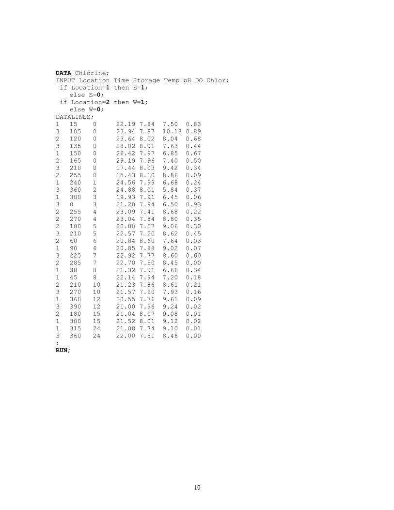
DATA Chlorine;

INPUT Location Time Storage Temp pH DO Chlor;

if Location=1 then E=1;

else E=0;

if Location=2 then W=1;

else W=0;

DATALINES;

1 15 0 22.19 7.84 7.50 0.83

3 105 0 23.94 7.97 10.13 0.89

2 120 0 23.64 8.02 8.04 0.68

3 135 0 28.02 8.01 7.63 0.44

1 150 0 26.42 7.97 6.85 0.67

2 165 0 29.19 7.96 7.40 0.50

3 210 0 17.44 8.03 9.42 0.34

2 255 0 15.43 8.10 8.86 0.09

1 240 1 24.56 7.99 6.68 0.24

3 360 2 24.88 8.01 5.84 0.37

1 300 3 19.93 7.91 6.45 0.06

3 0 3 21.20 7.94 6.50 0.93

2 255 4 23.09 7.41 8.68 0.22

2 270 4 23.04 7.84 8.80 0.35

2 180 5 20.80 7.57 9.06 0.30

3 210 5 22.57 7.20 8.62 0.45

2 60 6 20.84 8.60 7.64 0.03

1 90 6 20.85 7.88 9.02 0.07

3 225 7 22.92 7.77 8.60 0.60

2 285 7 22.70 7.50 8.45 0.00

1 30 8 21.32 7.91 6.66 0.34

1 45 8 22.14 7.94 7.20 0.18

2 210 10 21.23 7.86 8.61 0.21

3 270 10 21.57 7.90 7.93 0.16

1 360 12 20.55 7.76 9.61 0.09

3 390 12 21.00 7.96 9.24 0.02

2 180 15 21.04 8.07 9.08 0.01

1 300 15 21.52 8.01 9.12 0.02

1 315 24 21.08 7.74 9.10 0.01

3 360 24 22.00 7.51 8.46 0.00

;

RUN;

11

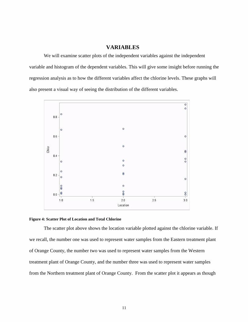
VARIABLES

We will examine scatter plots of the independent variables against the independent

variable and histogram of the dependent variables. This will give some insight before running the

regression analysis as to how the different variables affect the chlorine levels. These graphs will

also present a visual way of seeing the distribution of the different variables.

Figure 4: Scatter Plot of Location and Total Chlorine

The scatter plot above shows the location variable plotted against the chlorine variable. If

we recall, the number one was used to represent water samples from the Eastern treatment plant

of Orange County, the number two was used to represent water samples from the Western

treatment plant of Orange County, and the number three was used to represent water samples

from the Northern treatment plant of Orange County. From the scatter plot it appears as though

12

the Western treatment plant on average has the lowest chlorine levels. On the other hand, it

appears that the Northern treatment plant has the highest chlorine levels on average.

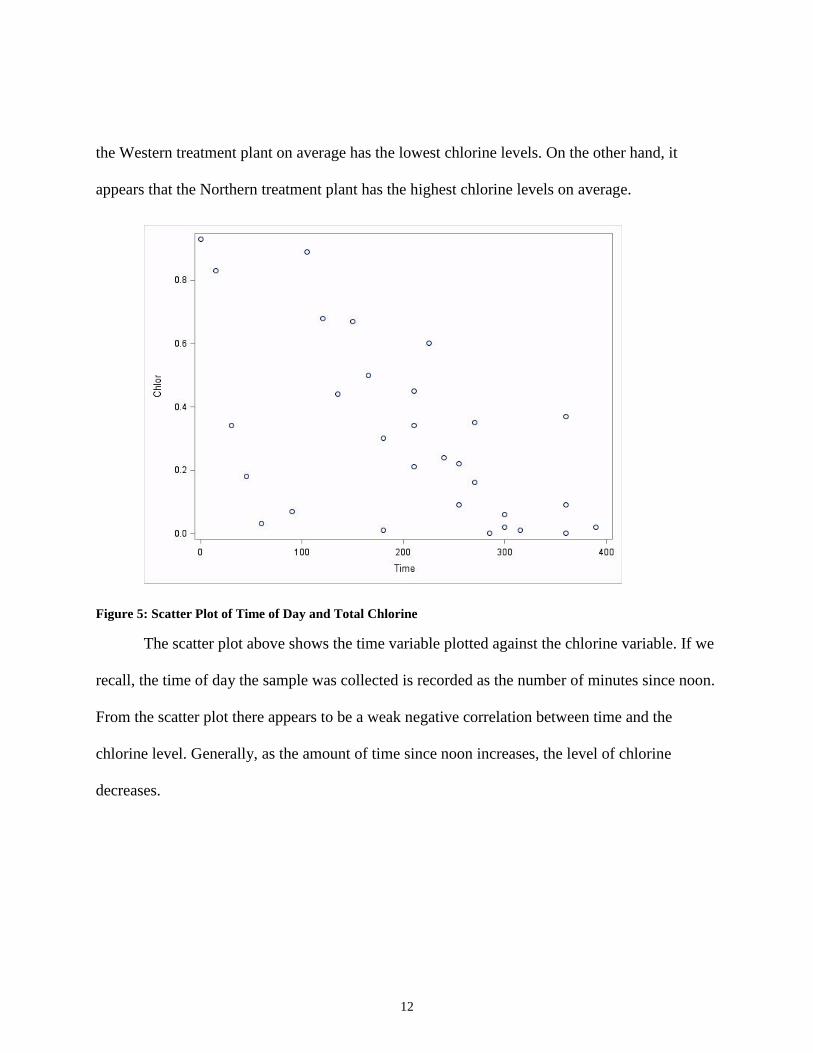
Figure 5: Scatter Plot of Time of Day and Total Chlorine

The scatter plot above shows the time variable plotted against the chlorine variable. If we

recall, the time of day the sample was collected is recorded as the number of minutes since noon.

From the scatter plot there appears to be a weak negative correlation between time and the

chlorine level. Generally, as the amount of time since noon increases, the level of chlorine

decreases.

13

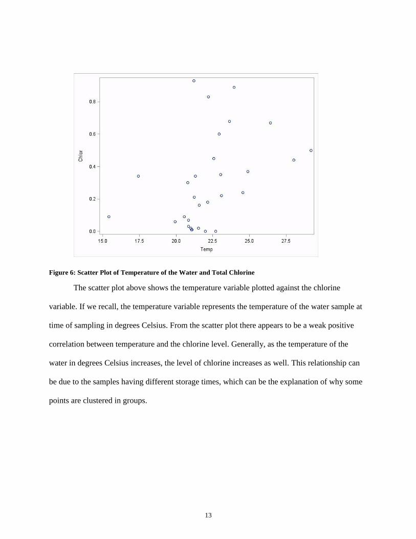
Figure 6: Scatter Plot of Temperature of the Water and Total Chlorine

The scatter plot above shows the temperature variable plotted against the chlorine

variable. If we recall, the temperature variable represents the temperature of the water sample at

time of sampling in degrees Celsius. From the scatter plot there appears to be a weak positive

correlation between temperature and the chlorine level. Generally, as the temperature of the

water in degrees Celsius increases, the level of chlorine increases as well. This relationship can

be due to the samples having different storage times, which can be the explanation of why some

points are clustered in groups.

14

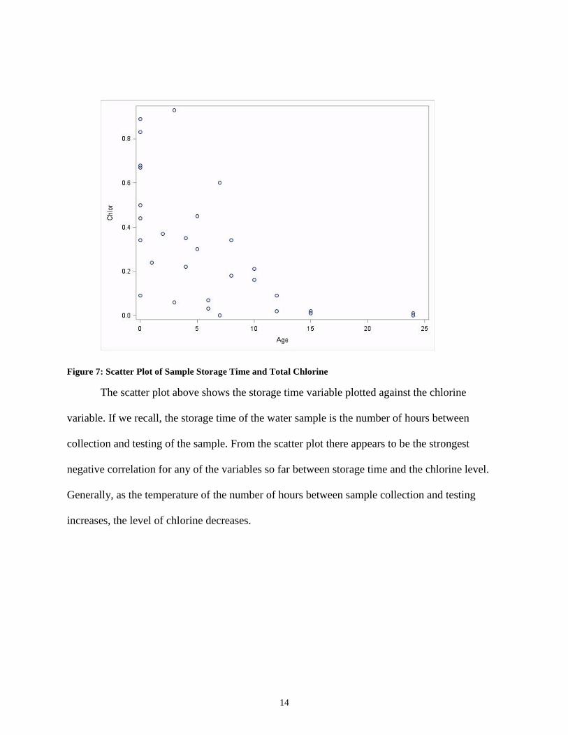
Figure 7: Scatter Plot of Sample Storage Time and Total Chlorine

The scatter plot above shows the storage time variable plotted against the chlorine

variable. If we recall, the storage time of the water sample is the number of hours between

collection and testing of the sample. From the scatter plot there appears to be the strongest

negative correlation for any of the variables so far between storage time and the chlorine level.

Generally, as the temperature of the number of hours between sample collection and testing

increases, the level of chlorine decreases.

15

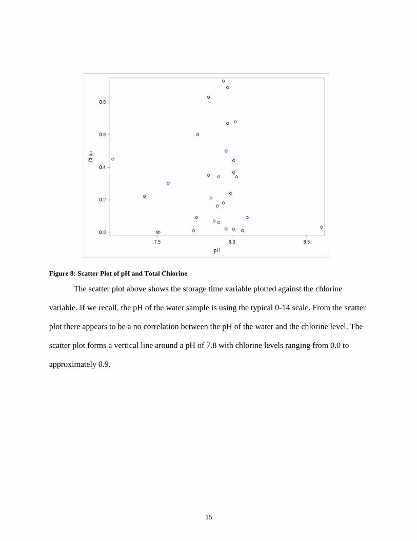
Figure 8: Scatter Plot of pH and Total Chlorine

The scatter plot above shows the storage time variable plotted against the chlorine

variable. If we recall, the pH of the water sample is using the typical 0-14 scale. From the scatter

plot there appears to be a no correlation between the pH of the water and the chlorine level. The

scatter plot forms a vertical line around a pH of 7.8 with chlorine levels ranging from 0.0 to

approximately 0.9.

16

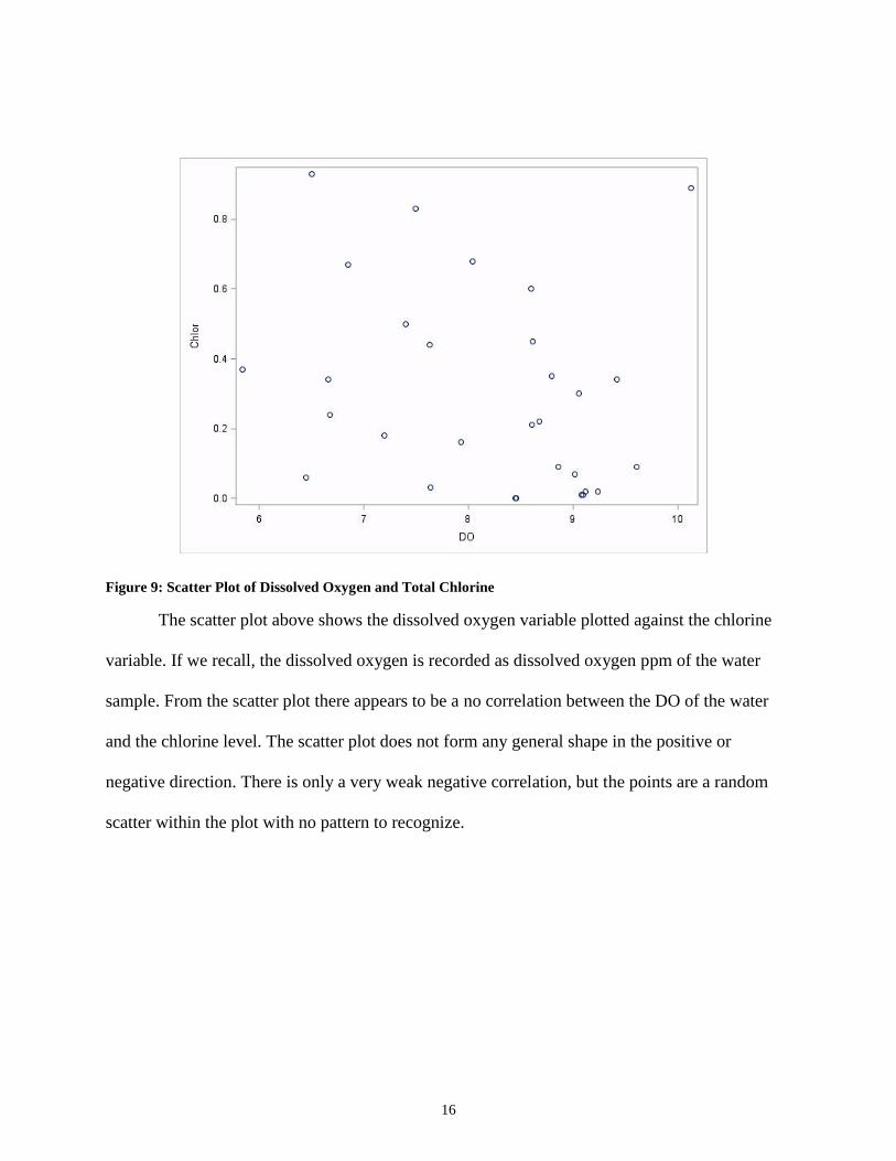
Figure 9: Scatter Plot of Dissolved Oxygen and Total Chlorine

The scatter plot above shows the dissolved oxygen variable plotted against the chlorine

variable. If we recall, the dissolved oxygen is recorded as dissolved oxygen ppm of the water

sample. From the scatter plot there appears to be a no correlation between the DO of the water

and the chlorine level. The scatter plot does not form any general shape in the positive or

negative direction. There is only a very weak negative correlation, but the points are a random

scatter within the plot with no pattern to recognize.

17

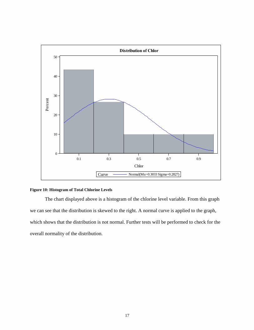
Figure 10: Histogram of Total Chlorine Levels

The chart displayed above is a histogram of the chlorine level variable. From this graph

we can see that the distribution is skewed to the right. A normal curve is applied to the graph,

which shows that the distribution is not normal. Further tests will be performed to check for the

overall normality of the distribution.

0.1 0.3 0.5 0.7 0.9

Chlor

0

10

20

30

40

50

Perc

ent

Normal(Mu=0.3033 Sigma=0.2827)Curve

Distribution of Chlor

18

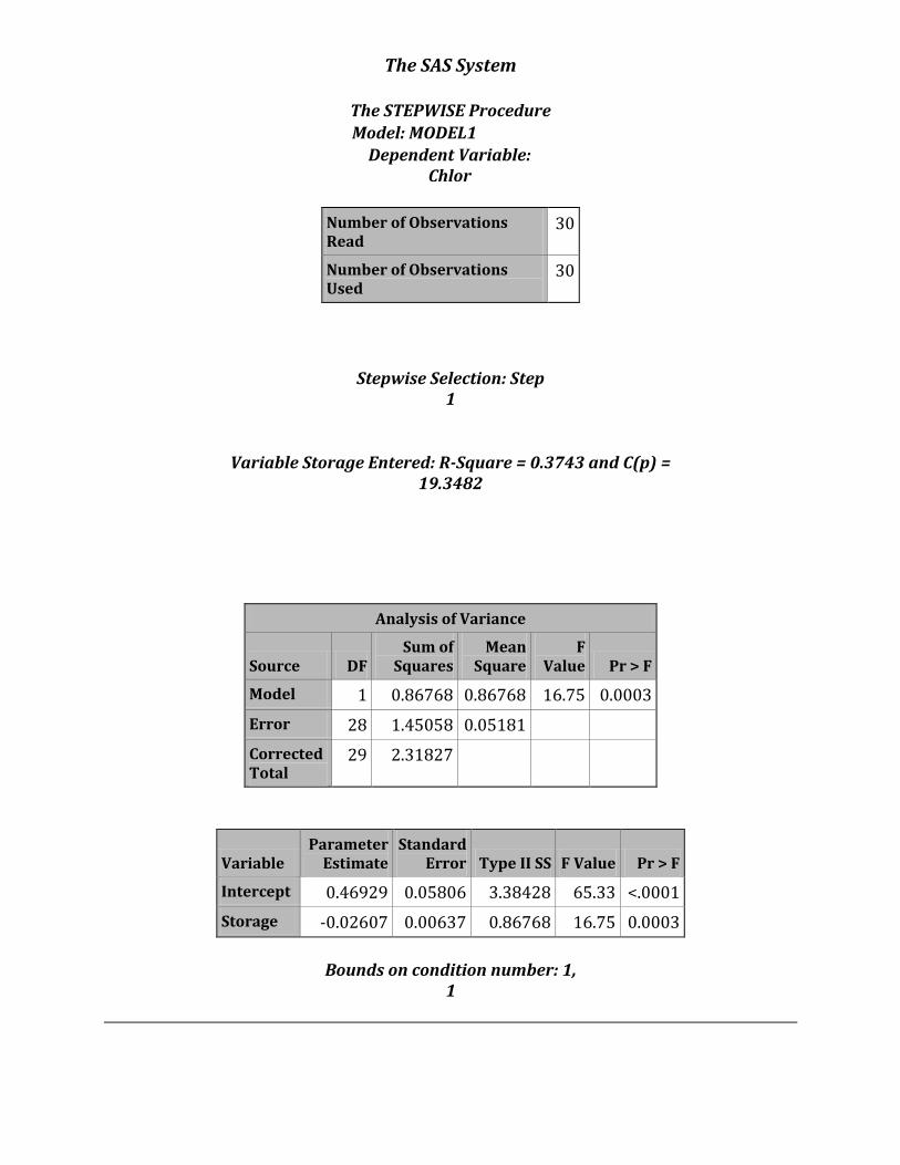
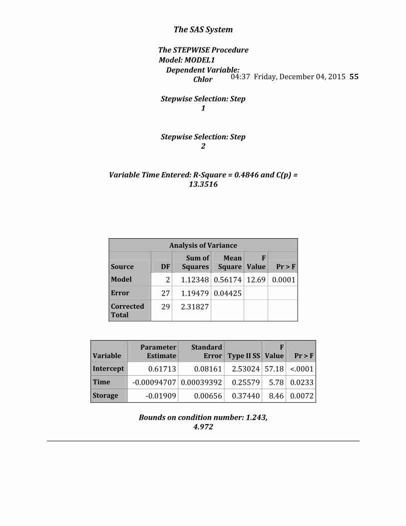
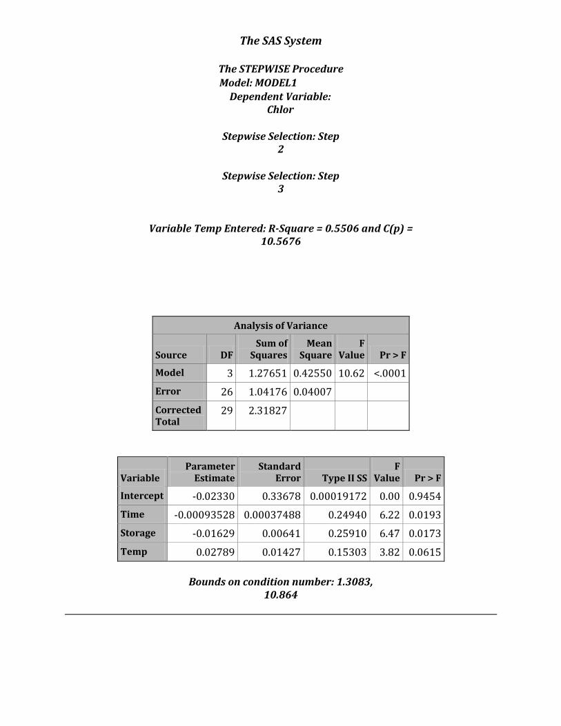
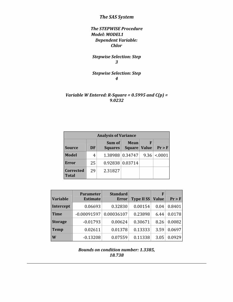
FINDING THE BEST MODEL

Through the stepwise selection method, the best model for this particular data will be

chosen. Stepwise, backward, and forward selection will all be used to see if they all select the

same model. In order to do so, PROC STEPWISE will be used. For this to work properly the

model must have the dependent variable, Chlor, in this instance, set equal to each independent

variable for which the user wants to include in the model. The model is followed by a forward

slash and the options of the type of model selection the user would like. For this analysis,

forward selection, backward elimination, and stepwise selection will be used, which means

forward, backward, and stepwise must be included in the options. If these options are not

included then the PROC will default to only running a stepwise selection. If the forward and

backward options are included but the stepwise option is not, then the PROC will only run a

forward selection and backward elimination. All three options should be included if the user

wants all three selection methods to be used. This method can be a bit more challenging when

working with dummy variables. Some users choose to run this PROC without incorporating the

dummy variables and then adding them to the chosen models. Other users will run the PROC

with the dummy variables and will add them to the model if all the dummy variables are not

selected, or, they will create new dummy variables depending on the selection. In this case, the

selection process is being run with the dummy variables and will be added to the model if only

one is selected.

PROC STEPWISE;

MODEL Chlor = Time Storage Temp pH DO E W / forward backward stepwise;

RUN;

19

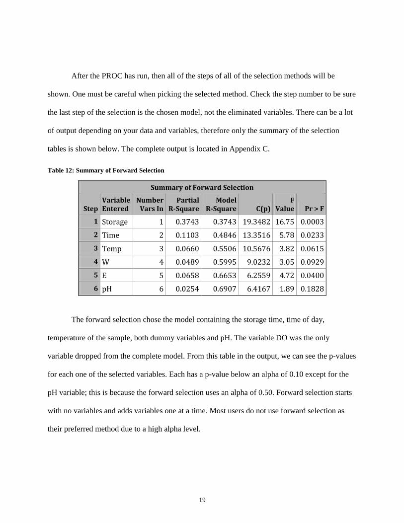
After the PROC has run, then all of the steps of all of the selection methods will be

shown. One must be careful when picking the selected method. Check the step number to be sure

the last step of the selection is the chosen model, not the eliminated variables. There can be a lot

of output depending on your data and variables, therefore only the summary of the selection

tables is shown below. The complete output is located in Appendix C.

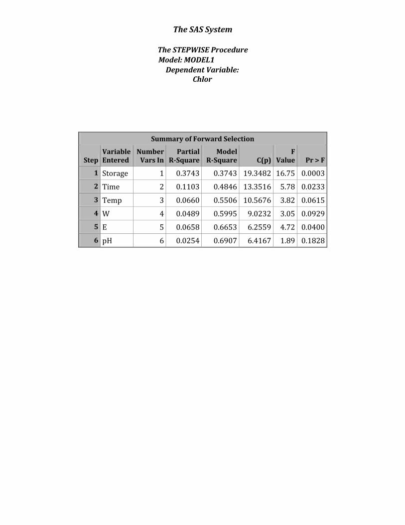
Table 12: Summary of Forward Selection

Summary of Forward Selection

Step Variable Entered

Number Vars In

Partial R-Square

Model R-Square C(p)

F Value Pr > F

1 Storage 1 0.3743 0.3743 19.3482 16.75 0.0003

2 Time 2 0.1103 0.4846 13.3516 5.78 0.0233

3 Temp 3 0.0660 0.5506 10.5676 3.82 0.0615

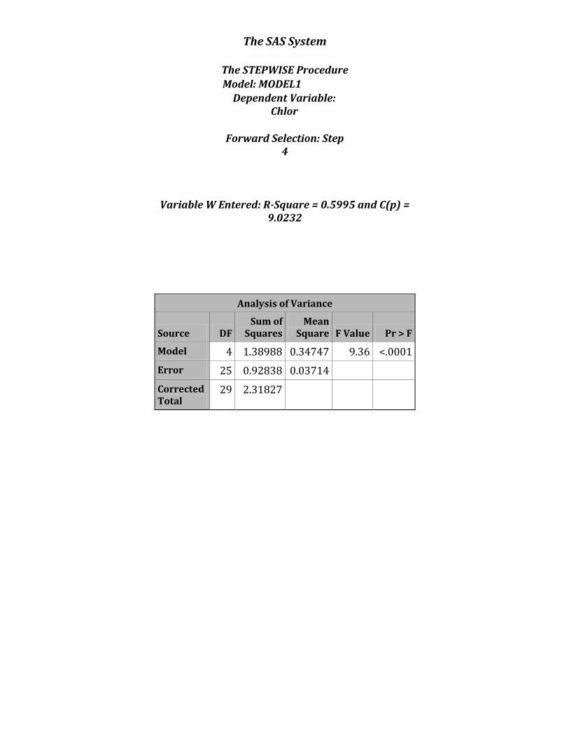
4 W 4 0.0489 0.5995 9.0232 3.05 0.0929

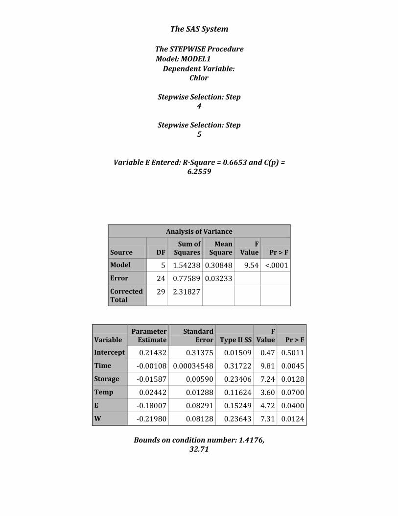
5 E 5 0.0658 0.6653 6.2559 4.72 0.0400

6 pH 6 0.0254 0.6907 6.4167 1.89 0.1828

The forward selection chose the model containing the storage time, time of day,

temperature of the sample, both dummy variables and pH. The variable DO was the only

variable dropped from the complete model. From this table in the output, we can see the p-values

for each one of the selected variables. Each has a p-value below an alpha of 0.10 except for the

pH variable; this is because the forward selection uses an alpha of 0.50. Forward selection starts

with no variables and adds variables one at a time. Most users do not use forward selection as

their preferred method due to a high alpha level.

20

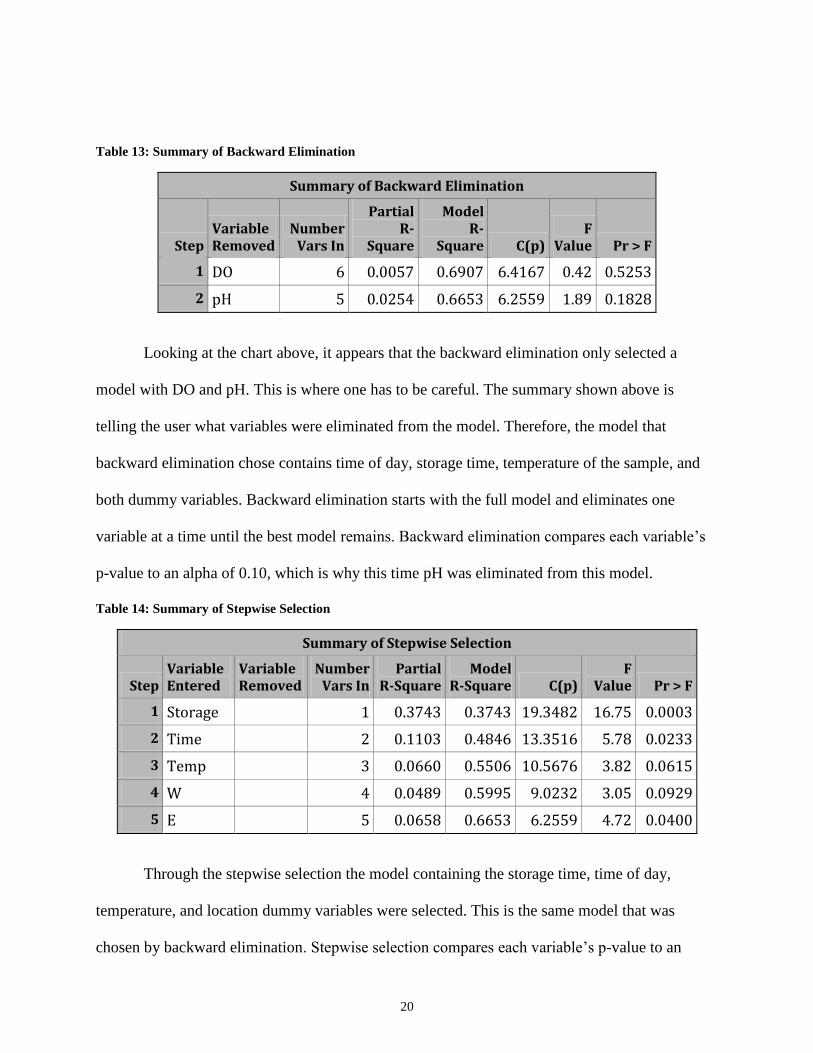
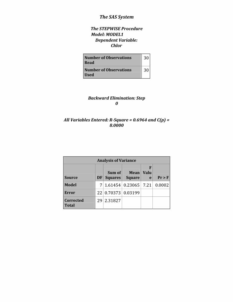
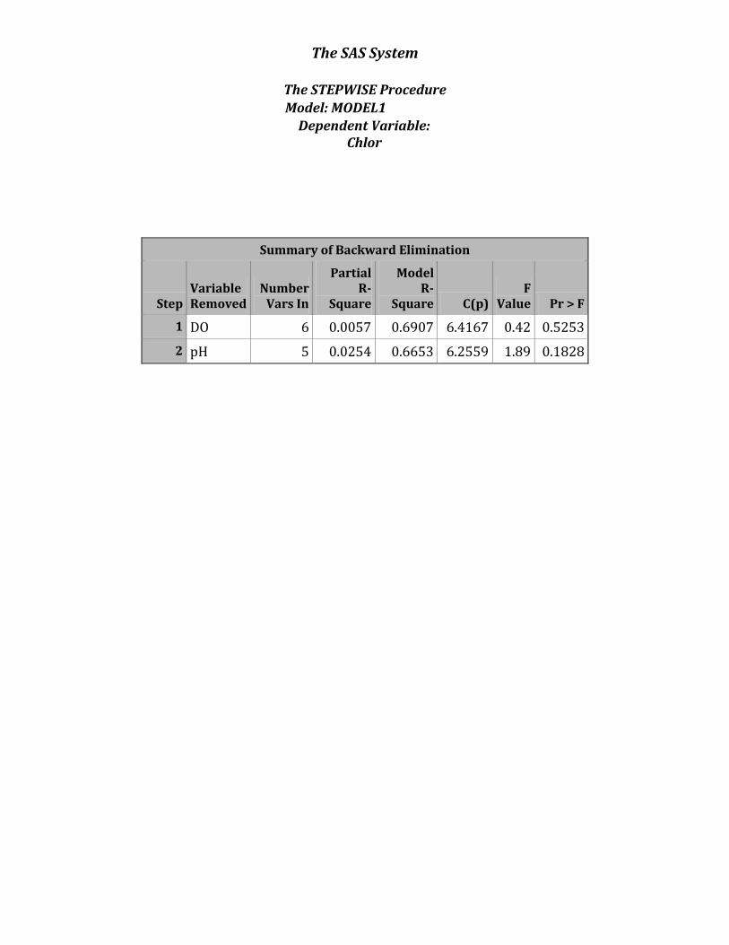
Table 13: Summary of Backward Elimination

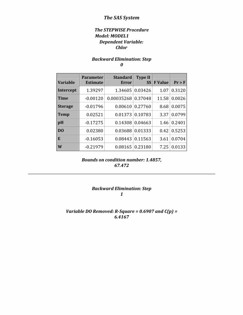
Summary of Backward Elimination

Step Variable Removed

Number Vars In

Partial R-

Square

Model R-

Square C(p) F

Value Pr > F

1 DO 6 0.0057 0.6907 6.4167 0.42 0.5253

2 pH 5 0.0254 0.6653 6.2559 1.89 0.1828

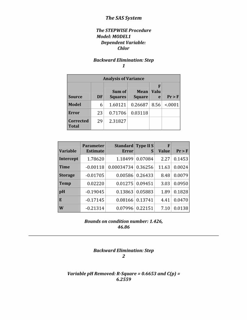
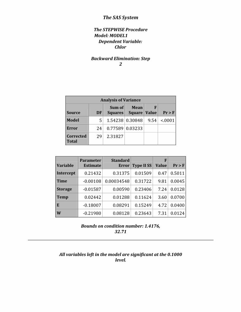
Looking at the chart above, it appears that the backward elimination only selected a

model with DO and pH. This is where one has to be careful. The summary shown above is

telling the user what variables were eliminated from the model. Therefore, the model that

backward elimination chose contains time of day, storage time, temperature of the sample, and

both dummy variables. Backward elimination starts with the full model and eliminates one

variable at a time until the best model remains. Backward elimination compares each variable’s

p-value to an alpha of 0.10, which is why this time pH was eliminated from this model.

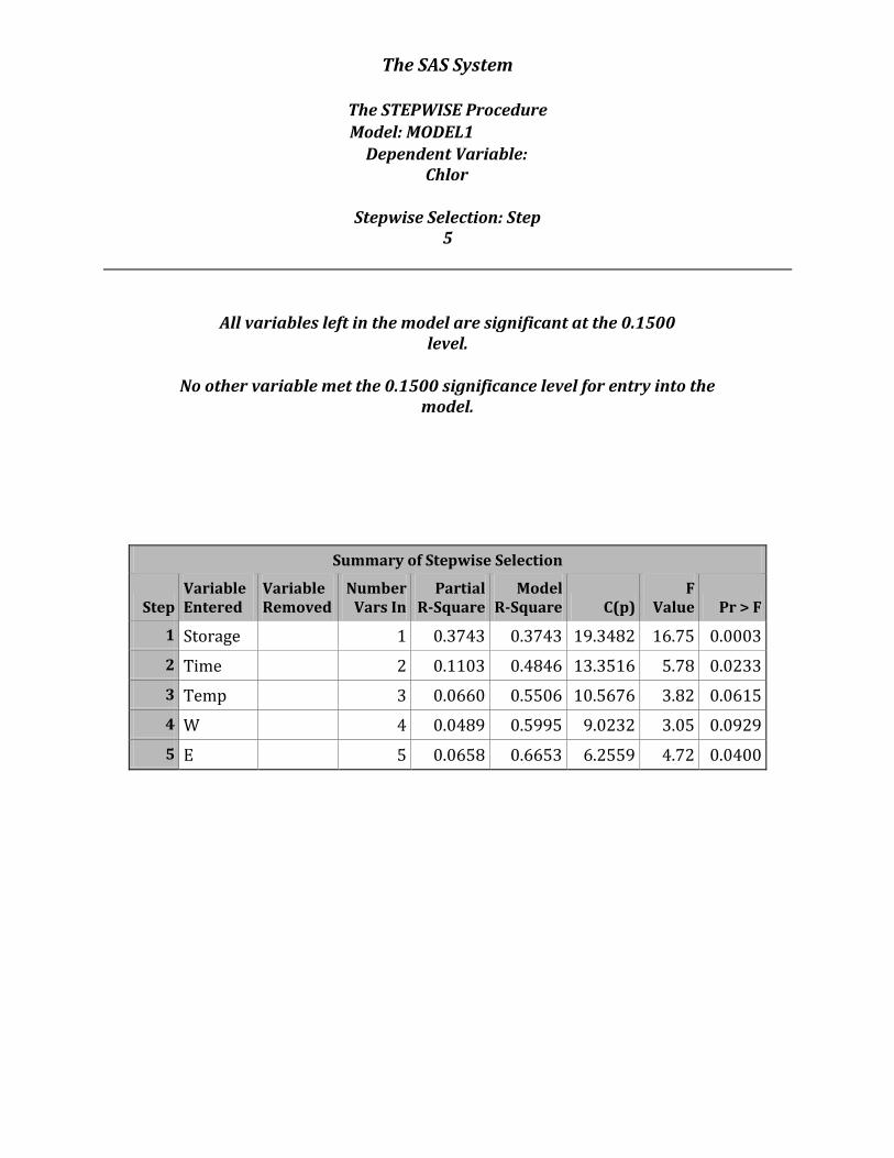
Table 14: Summary of Stepwise Selection

Summary of Stepwise Selection


Variable Removed

Number Vars In

Partial R-Square

Model R-Square C(p)

F Value Pr > F

1 Storage 1 0.3743 0.3743 19.3482 16.75 0.0003

2 Time 2 0.1103 0.4846 13.3516 5.78 0.0233

3 Temp 3 0.0660 0.5506 10.5676 3.82 0.0615

4 W 4 0.0489 0.5995 9.0232 3.05 0.0929

5 E 5 0.0658 0.6653 6.2559 4.72 0.0400

Through the stepwise selection the model containing the storage time, time of day,

temperature, and location dummy variables were selected. This is the same model that was

chosen by backward elimination. Stepwise selection compares each variable’s p-value to an

21

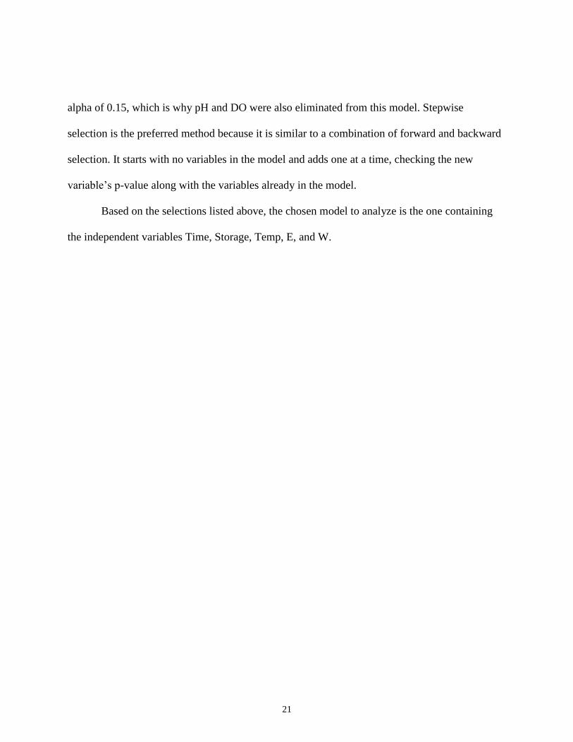
alpha of 0.15, which is why pH and DO were also eliminated from this model. Stepwise

selection is the preferred method because it is similar to a combination of forward and backward

selection. It starts with no variables in the model and adds one at a time, checking the new

variable’s p-value along with the variables already in the model.

Based on the selections listed above, the chosen model to analyze is the one containing

the independent variables Time, Storage, Temp, E, and W.

22

ANALYZING THE CHOSEN MODEL

In order to see if this model is useful we must check and analyze the conditions necessary

for this to be true. A global F test will be done to see if the model is deemed useful. We will also

investigate residual plots, jackknife residuals, leverage values, Cook’s D, PRESS statistic, and

normal probability plot of the residuals. Possible outliers will be flagged based on these findings.

We will also look into any problems with collinearity between the variables. This will all be

done using the code below.

PROC REG;

model Chlor = Time Storage Temp E W / partial influence VIF;

output out=new cookd=cook rstudent=jack h=lev r=resid;

RUN;

PROC PRINT data= new;

RUN;

PROC UNIVARIATE normal plot;

var resid;

RUN;

PROC CORR;

var Time Storage Temp E W;

RUN;

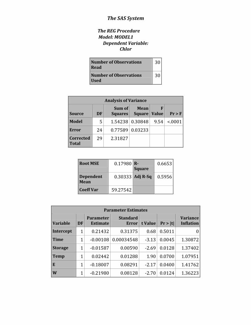
F Test

Through PROC REG with the previously selected model one is able to perform a global F test on

the model to test its significance.

23

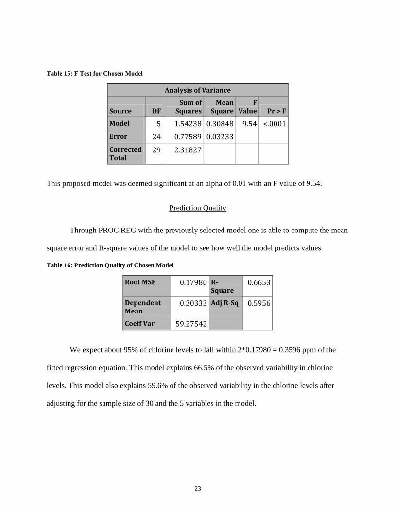
Table 15: F Test for Chosen Model

Analysis of Variance

Source DF Sum of

Squares Mean

Square F

Value Pr > F

Model 5 1.54238 0.30848 9.54 <.0001

Error 24 0.77589 0.03233

Corrected Total

29 2.31827

This proposed model was deemed significant at an alpha of 0.01 with an F value of 9.54.

Prediction Quality

Through PROC REG with the previously selected model one is able to compute the mean

square error and R-square values of the model to see how well the model predicts values.

Table 16: Prediction Quality of Chosen Model

Root MSE 0.17980 R-Square

0.6653

Dependent Mean

0.30333 Adj R-Sq 0.5956

Coeff Var 59.27542

We expect about 95% of chlorine levels to fall within 2*0.17980 = 0.3596 ppm of the

fitted regression equation. This model explains 66.5% of the observed variability in chlorine

levels. This model also explains 59.6% of the observed variability in the chlorine levels after

adjusting for the sample size of 30 and the 5 variables in the model.

24

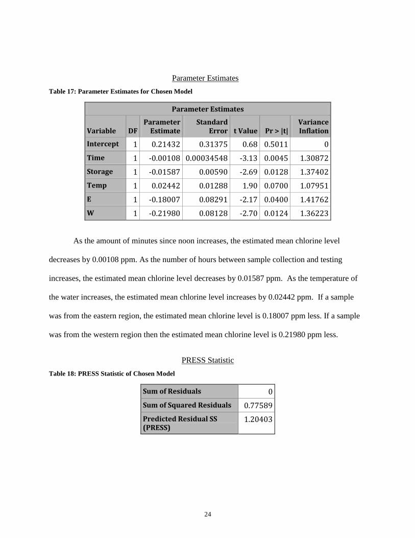
Parameter Estimates

Table 17: Parameter Estimates for Chosen Model

Parameter Estimates

Variable DF Parameter

Estimate Standard

Error t Value Pr > |t| Variance Inflation

Intercept 1 0.21432 0.31375 0.68 0.5011 0

Time 1 -0.00108 0.00034548 -3.13 0.0045 1.30872

Storage 1 -0.01587 0.00590 -2.69 0.0128 1.37402

Temp 1 0.02442 0.01288 1.90 0.0700 1.07951

E 1 -0.18007 0.08291 -2.17 0.0400 1.41762

W 1 -0.21980 0.08128 -2.70 0.0124 1.36223

As the amount of minutes since noon increases, the estimated mean chlorine level

decreases by 0.00108 ppm. As the number of hours between sample collection and testing

increases, the estimated mean chlorine level decreases by 0.01587 ppm. As the temperature of

the water increases, the estimated mean chlorine level increases by 0.02442 ppm. If a sample

was from the eastern region, the estimated mean chlorine level is 0.18007 ppm less. If a sample

was from the western region then the estimated mean chlorine level is 0.21980 ppm less.

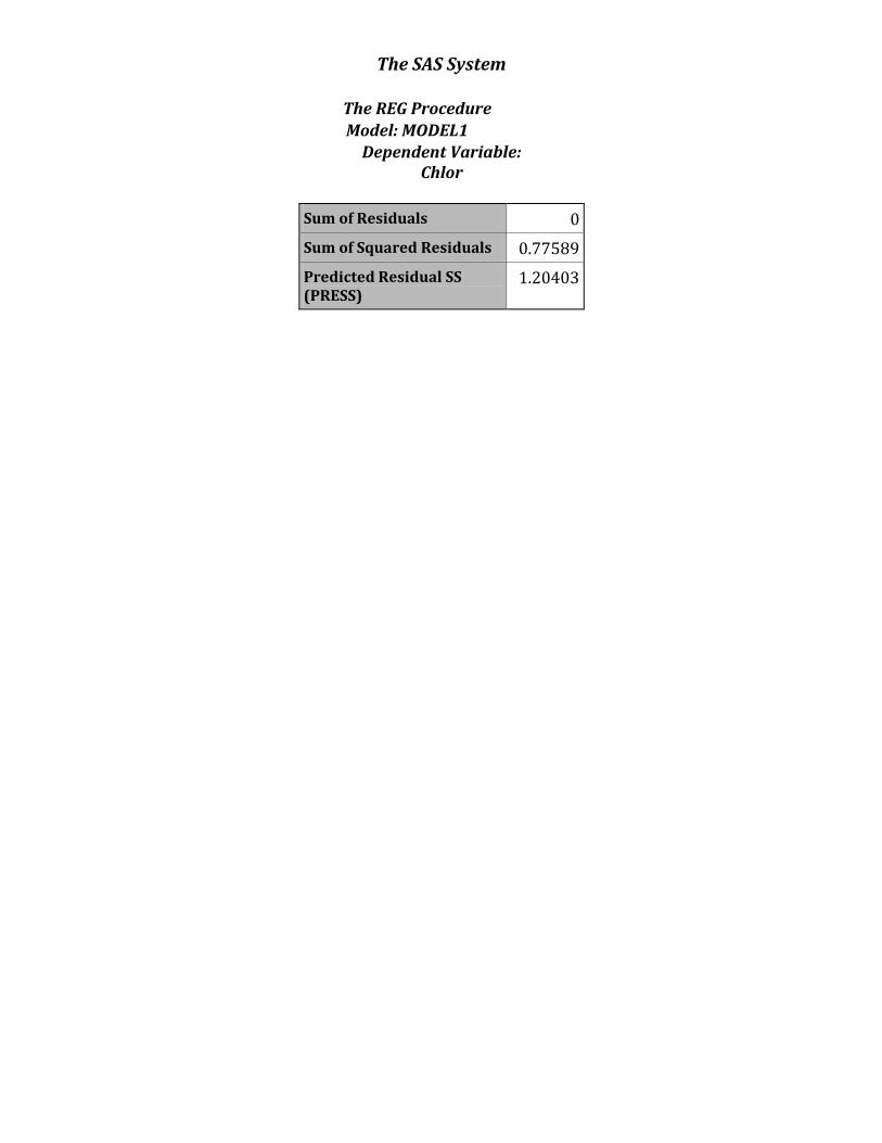
PRESS Statistic

Table 18: PRESS Statistic of Chosen Model

Sum of Residuals 0

Sum of Squared Residuals 0.77589

Predicted Residual SS (PRESS)

1.20403

25

It is ideal to have a small PRESS statistic value and in this particular case the PRESS

statistic is 1.20. The PRESS statistic is similar to the R-square value in respect to saying how

well the model explains the observed variability.

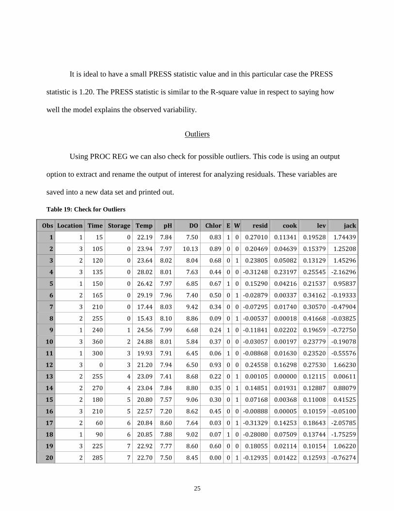
Outliers

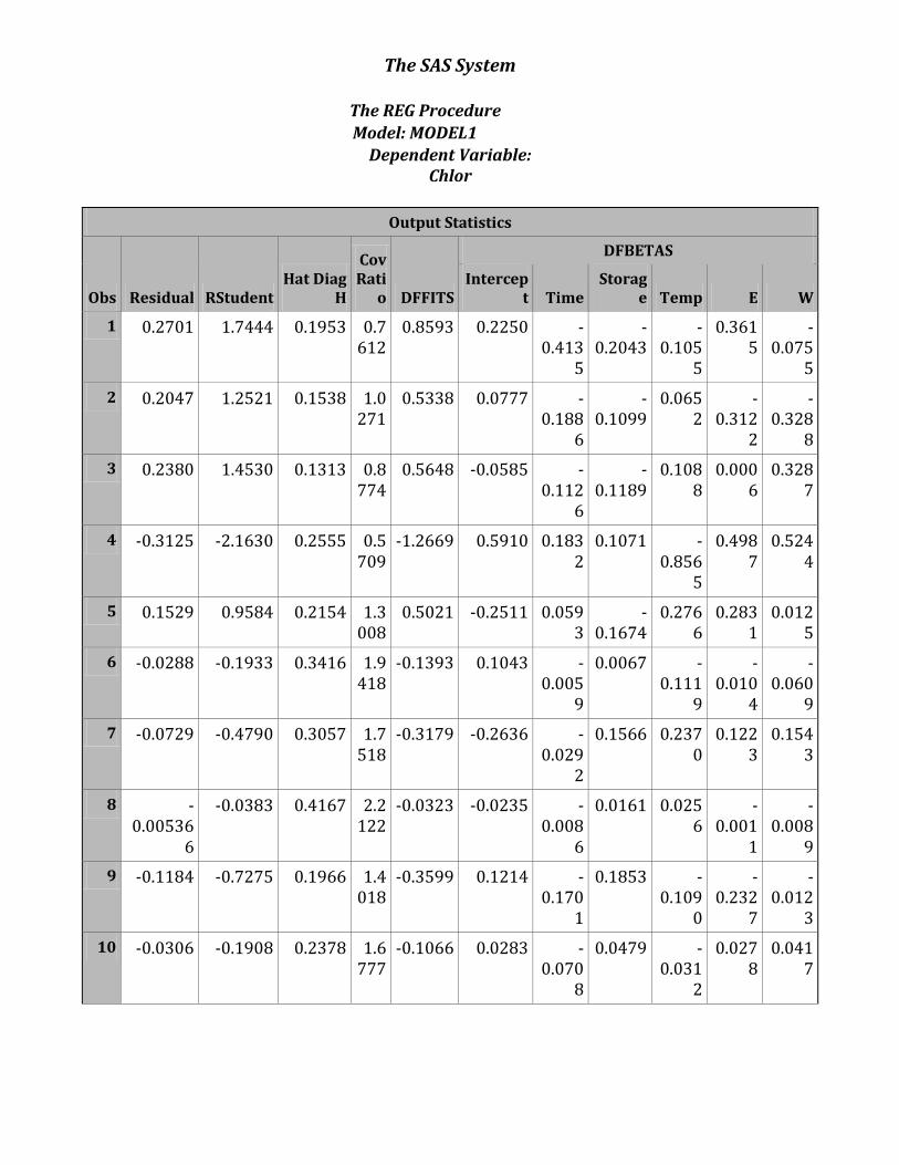
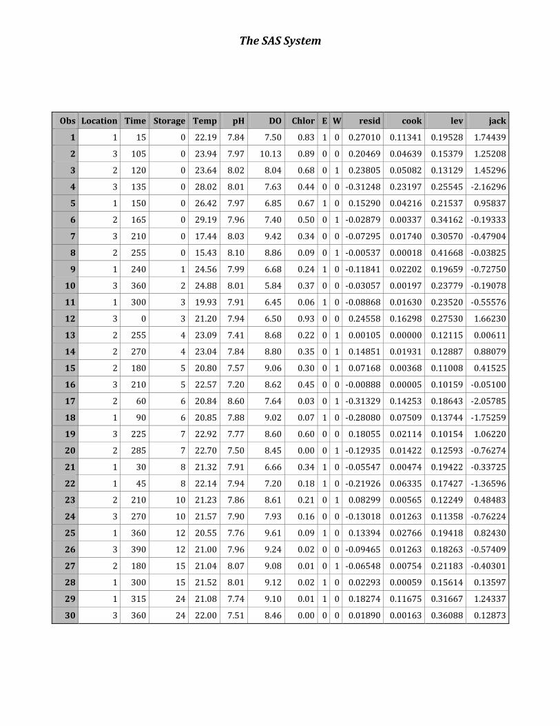
Using PROC REG we can also check for possible outliers. This code is using an output

option to extract and rename the output of interest for analyzing residuals. These variables are

saved into a new data set and printed out.

Table 19: Check for Outliers

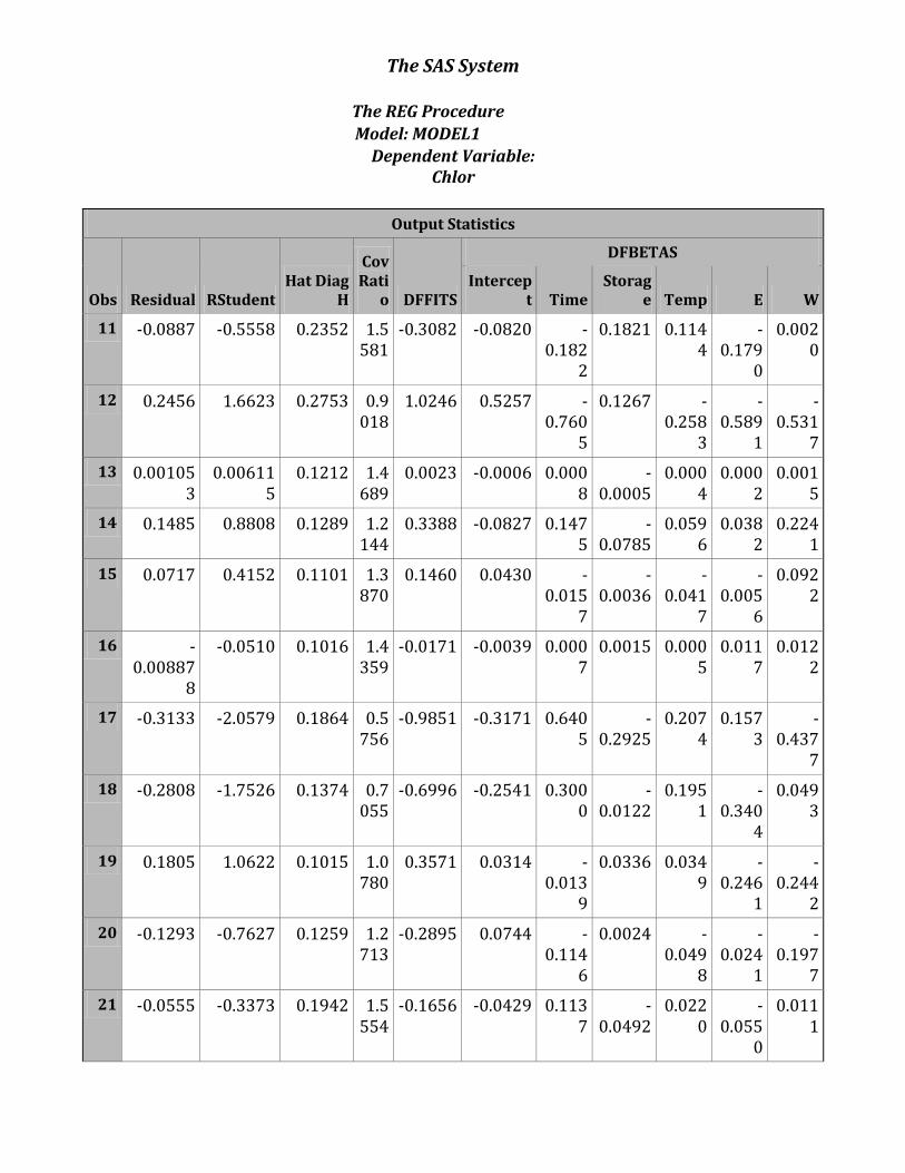
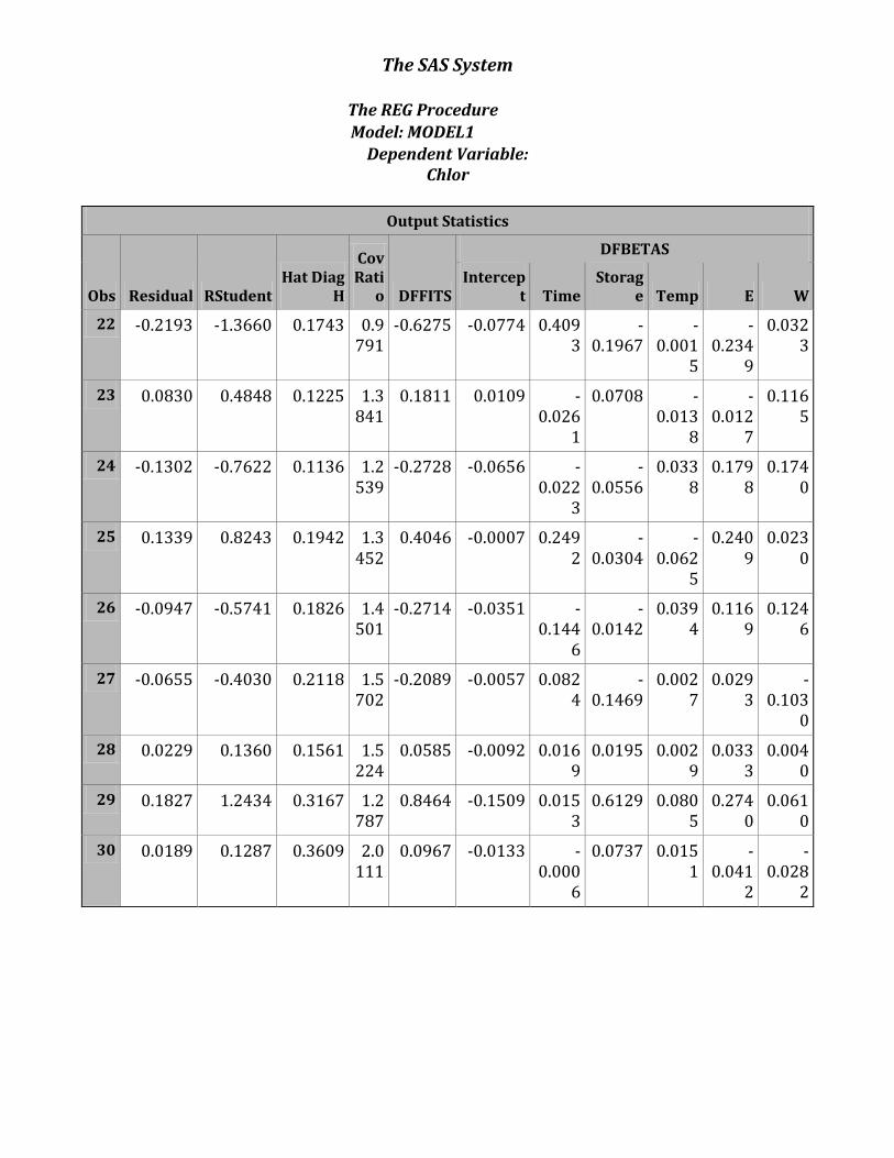
Obs Location Time Storage Temp pH DO Chlor E W resid cook lev jack

1 1 15 0 22.19 7.84 7.50 0.83 1 0 0.27010 0.11341 0.19528 1.74439

2 3 105 0 23.94 7.97 10.13 0.89 0 0 0.20469 0.04639 0.15379 1.25208

3 2 120 0 23.64 8.02 8.04 0.68 0 1 0.23805 0.05082 0.13129 1.45296

4 3 135 0 28.02 8.01 7.63 0.44 0 0 -0.31248 0.23197 0.25545 -2.16296

5 1 150 0 26.42 7.97 6.85 0.67 1 0 0.15290 0.04216 0.21537 0.95837

6 2 165 0 29.19 7.96 7.40 0.50 0 1 -0.02879 0.00337 0.34162 -0.19333

7 3 210 0 17.44 8.03 9.42 0.34 0 0 -0.07295 0.01740 0.30570 -0.47904

8 2 255 0 15.43 8.10 8.86 0.09 0 1 -0.00537 0.00018 0.41668 -0.03825

9 1 240 1 24.56 7.99 6.68 0.24 1 0 -0.11841 0.02202 0.19659 -0.72750

10 3 360 2 24.88 8.01 5.84 0.37 0 0 -0.03057 0.00197 0.23779 -0.19078

11 1 300 3 19.93 7.91 6.45 0.06 1 0 -0.08868 0.01630 0.23520 -0.55576

12 3 0 3 21.20 7.94 6.50 0.93 0 0 0.24558 0.16298 0.27530 1.66230

13 2 255 4 23.09 7.41 8.68 0.22 0 1 0.00105 0.00000 0.12115 0.00611

14 2 270 4 23.04 7.84 8.80 0.35 0 1 0.14851 0.01931 0.12887 0.88079

15 2 180 5 20.80 7.57 9.06 0.30 0 1 0.07168 0.00368 0.11008 0.41525

16 3 210 5 22.57 7.20 8.62 0.45 0 0 -0.00888 0.00005 0.10159 -0.05100

17 2 60 6 20.84 8.60 7.64 0.03 0 1 -0.31329 0.14253 0.18643 -2.05785

18 1 90 6 20.85 7.88 9.02 0.07 1 0 -0.28080 0.07509 0.13744 -1.75259

19 3 225 7 22.92 7.77 8.60 0.60 0 0 0.18055 0.02114 0.10154 1.06220

20 2 285 7 22.70 7.50 8.45 0.00 0 1 -0.12935 0.01422 0.12593 -0.76274

26


21 1 30 8 21.32 7.91 6.66 0.34 1 0 -0.05547 0.00474 0.19422 -0.33725

22 1 45 8 22.14 7.94 7.20 0.18 1 0 -0.21926 0.06335 0.17427 -1.36596

23 2 210 10 21.23 7.86 8.61 0.21 0 1 0.08299 0.00565 0.12249 0.48483

24 3 270 10 21.57 7.90 7.93 0.16 0 0 -0.13018 0.01263 0.11358 -0.76224

25 1 360 12 20.55 7.76 9.61 0.09 1 0 0.13394 0.02766 0.19418 0.82430

26 3 390 12 21.00 7.96 9.24 0.02 0 0 -0.09465 0.01263 0.18263 -0.57409

27 2 180 15 21.04 8.07 9.08 0.01 0 1 -0.06548 0.00754 0.21183 -0.40301

28 1 300 15 21.52 8.01 9.12 0.02 1 0 0.02293 0.00059 0.15614 0.13597

29 1 315 24 21.08 7.74 9.10 0.01 1 0 0.18274 0.11675 0.31667 1.24337

30 3 360 24 22.00 7.51 8.46 0.00 0 0 0.01890 0.00163 0.36088 0.12873

An observation is flagged is their leverage is greater than 2(k+1)/n = 0.67. An

observation is flagged if their jackknife residual value is less than a negative t critical with

alpha/2n and degrees of freedom equal to n-k-1 or greater than a positive t critical with alpha/2n

and degrees of freedom equal to n-k-1. No jackknife residual values were less than -3.56 or

greater than 3.56. As a general rule of thumb, if the Cook’s D value is greater than 1.00, the

observation is influential. No Cook’s D values were greater than 1.00. There were no

observations that were flagged as possible outliers with respect to the dependent or independent

variables.

27

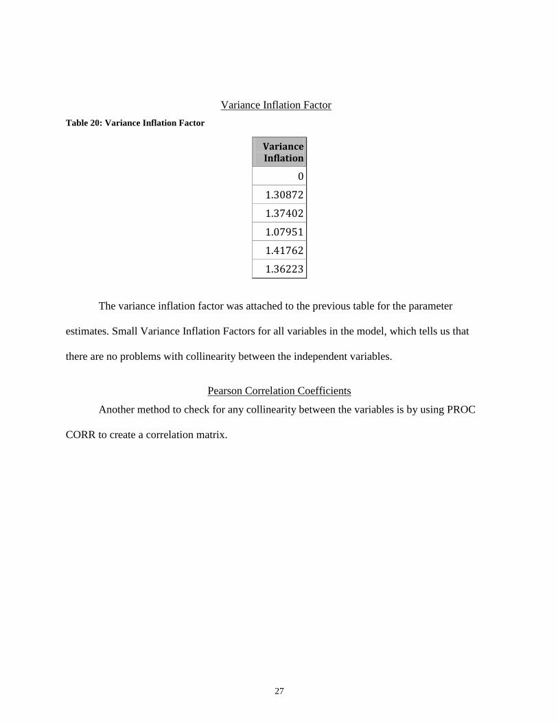
Variance Inflation Factor

Table 20: Variance Inflation Factor

Variance Inflation

0

1.30872

1.37402

1.07951

1.41762

1.36223

The variance inflation factor was attached to the previous table for the parameter

estimates. Small Variance Inflation Factors for all variables in the model, which tells us that

there are no problems with collinearity between the independent variables.

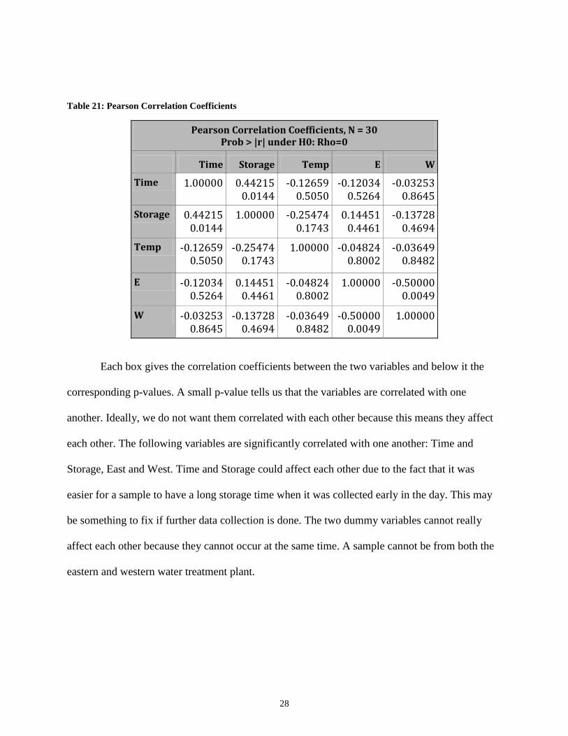
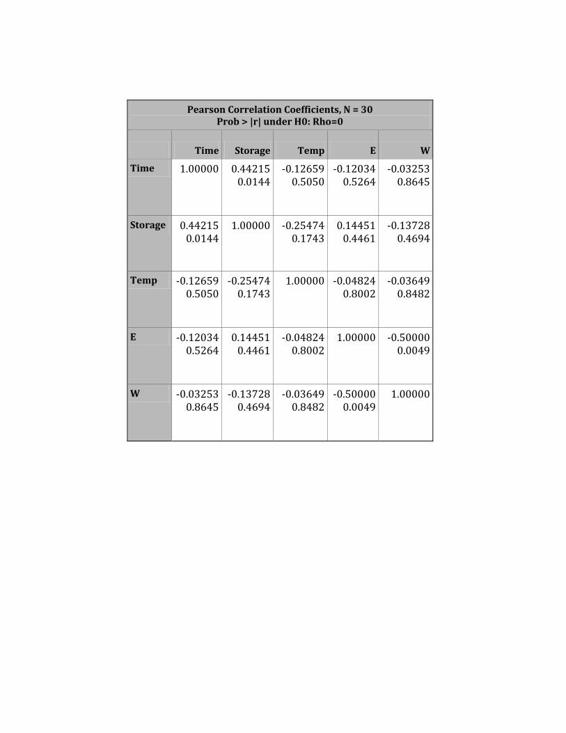
Pearson Correlation Coefficients

Another method to check for any collinearity between the variables is by using PROC

CORR to create a correlation matrix.

28

Table 21: Pearson Correlation Coefficients

Pearson Correlation Coefficients, N = 30 Prob > |r| under H0: Rho=0

Time Storage Temp E W

Time 1.00000

0.44215 0.0144

-0.12659 0.5050

-0.12034 0.5264

-0.03253 0.8645

Storage 0.44215 0.0144

1.00000

-0.25474 0.1743

0.14451 0.4461

-0.13728 0.4694

Temp -0.12659 0.5050

-0.25474 0.1743

1.00000

-0.04824 0.8002

-0.03649 0.8482

E -0.12034 0.5264

0.14451 0.4461

-0.04824 0.8002

1.00000

-0.50000 0.0049

W -0.03253 0.8645

-0.13728 0.4694

-0.03649 0.8482

-0.50000 0.0049

1.00000

Each box gives the correlation coefficients between the two variables and below it the

corresponding p-values. A small p-value tells us that the variables are correlated with one

another. Ideally, we do not want them correlated with each other because this means they affect

each other. The following variables are significantly correlated with one another: Time and

Storage, East and West. Time and Storage could affect each other due to the fact that it was

easier for a sample to have a long storage time when it was collected early in the day. This may

be something to fix if further data collection is done. The two dummy variables cannot really

affect each other because they cannot occur at the same time. A sample cannot be from both the

eastern and western water treatment plant.

29

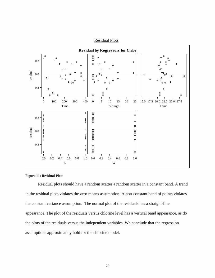
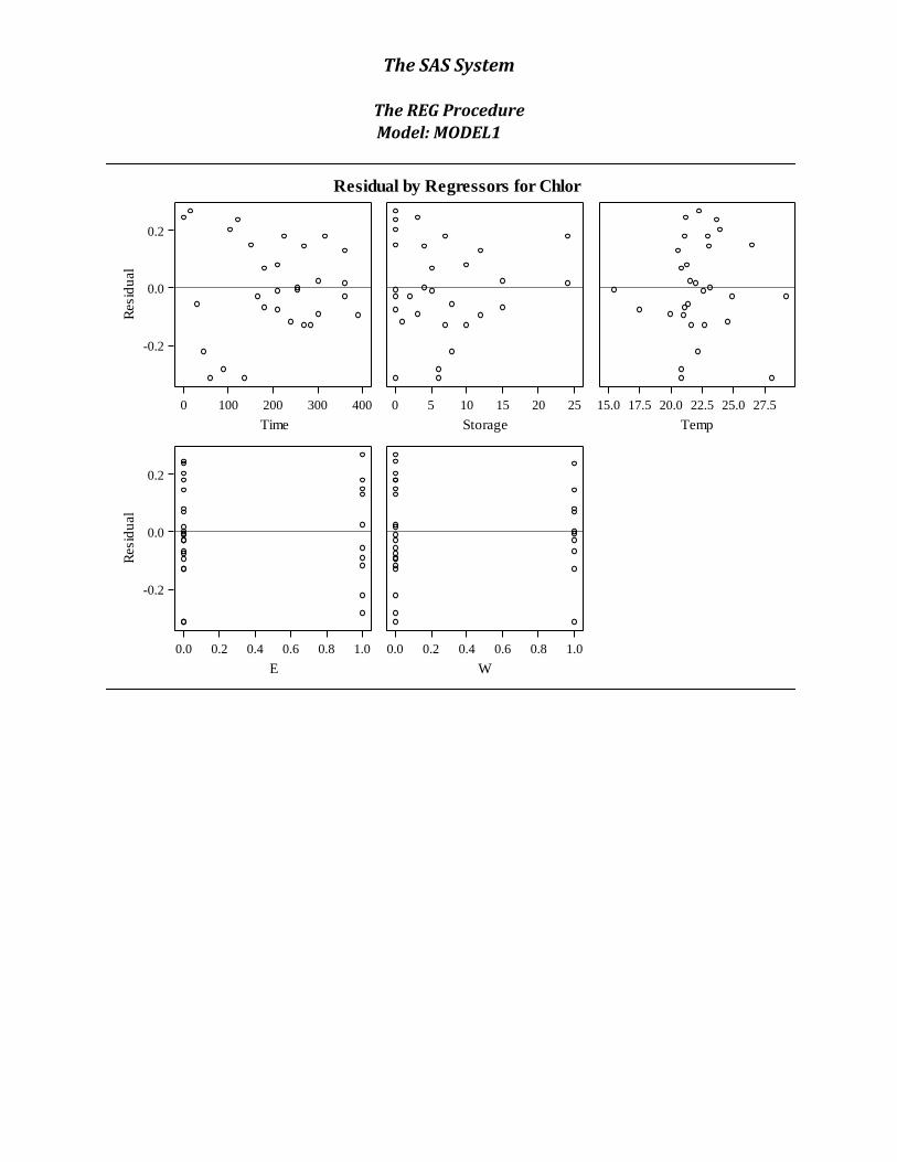
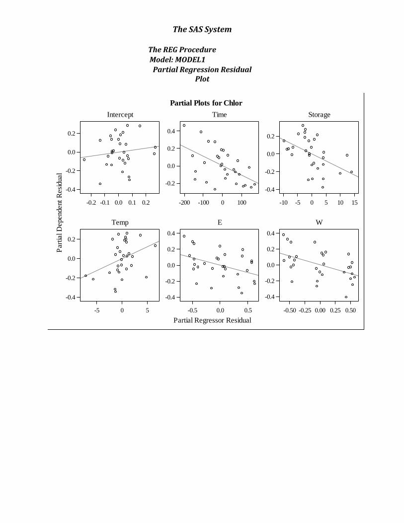
Residual Plots

Figure 11: Residual Plots

Residual plots should have a random scatter a random scatter in a constant band. A trend

in the residual plots violates the zero means assumption. A non-constant band of points violates

the constant variance assumption. The normal plot of the residuals has a straight-line

appearance. The plot of the residuals versus chlorine level has a vertical band appearance, as do

the plots of the residuals versus the independent variables. We conclude that the regression

assumptions approximately hold for the chlorine model.

Residual by Regressors for Chlor

0.0 0.2 0.4 0.6 0.8 1.0

W

0.0 0.2 0.4 0.6 0.8 1.0

E

15.0 17.5 20.0 22.5 25.0 27.5

Temp

0 5 10 15 20 25

Storage

0 100 200 300 400

Time

-0.2

0.0

0.2

Resid

ual

-0.2

0.0

0.2

Resid

ual

30

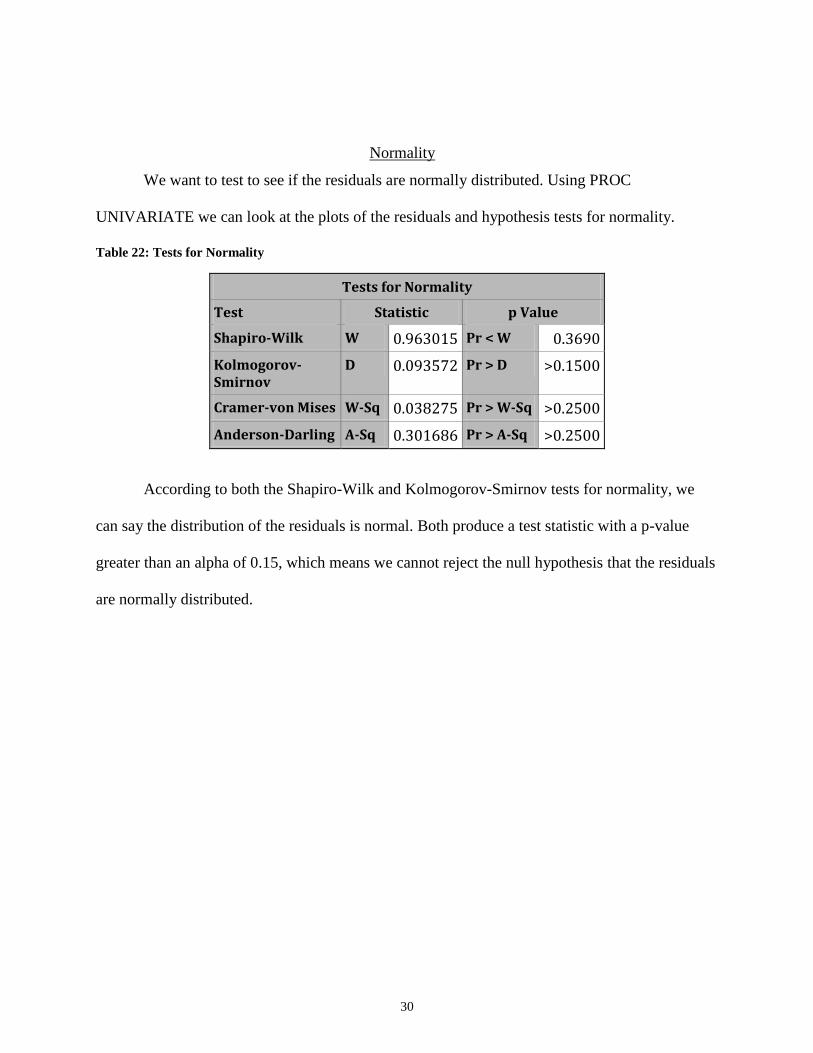
Normality

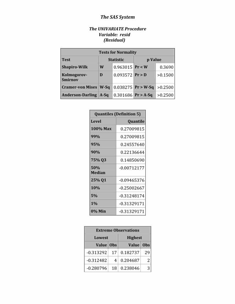
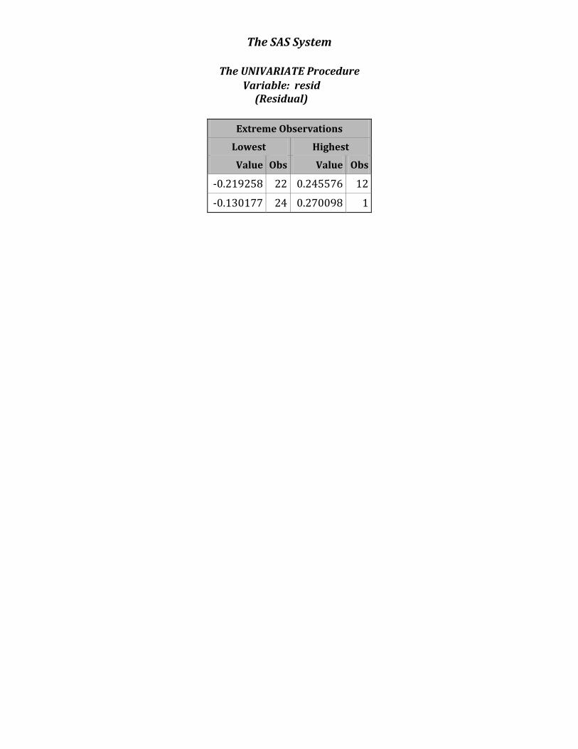
We want to test to see if the residuals are normally distributed. Using PROC

UNIVARIATE we can look at the plots of the residuals and hypothesis tests for normality.

Table 22: Tests for Normality

Tests for Normality

Test Statistic p Value

Shapiro-Wilk W 0.963015 Pr < W 0.3690

Kolmogorov-Smirnov

D 0.093572 Pr > D >0.1500

Cramer-von Mises W-Sq 0.038275 Pr > W-Sq >0.2500

Anderson-Darling A-Sq 0.301686 Pr > A-Sq >0.2500

According to both the Shapiro-Wilk and Kolmogorov-Smirnov tests for normality, we

can say the distribution of the residuals is normal. Both produce a test statistic with a p-value

greater than an alpha of 0.15, which means we cannot reject the null hypothesis that the residuals

are normally distributed.

31

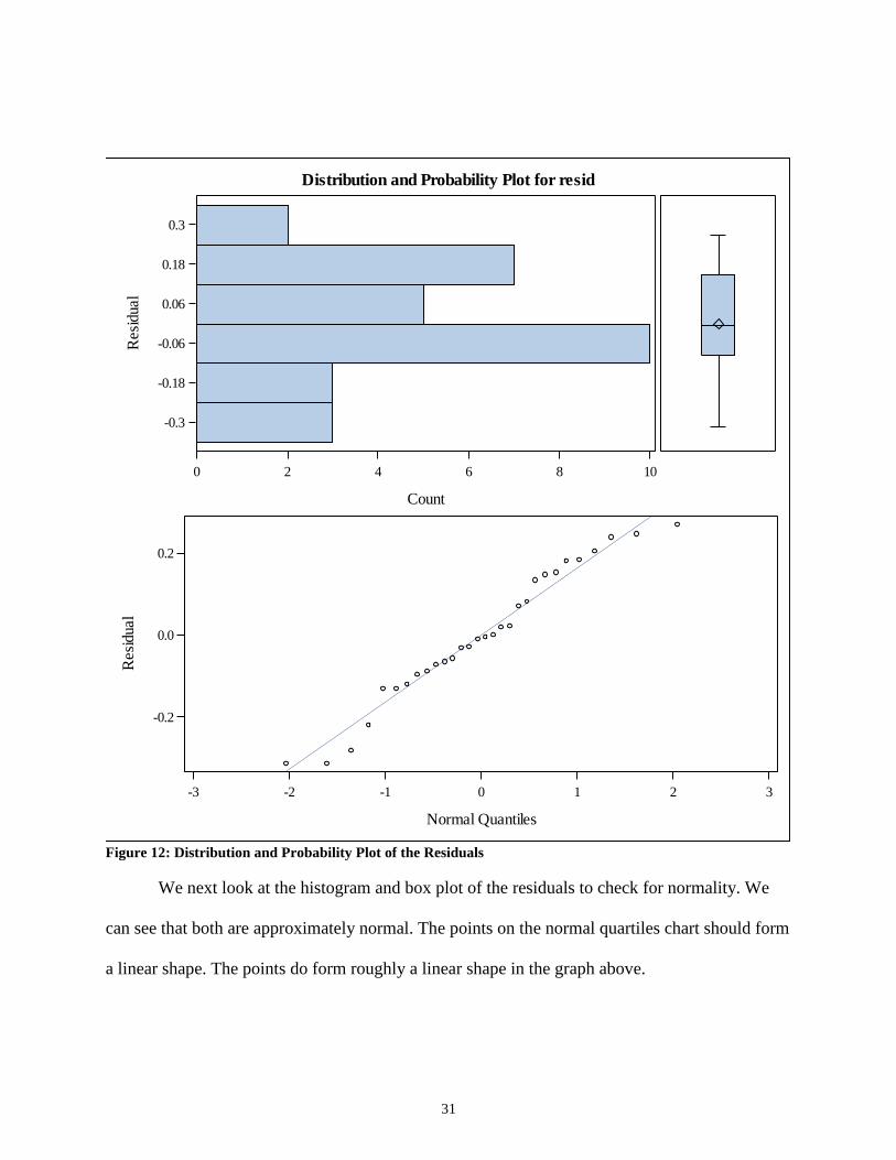
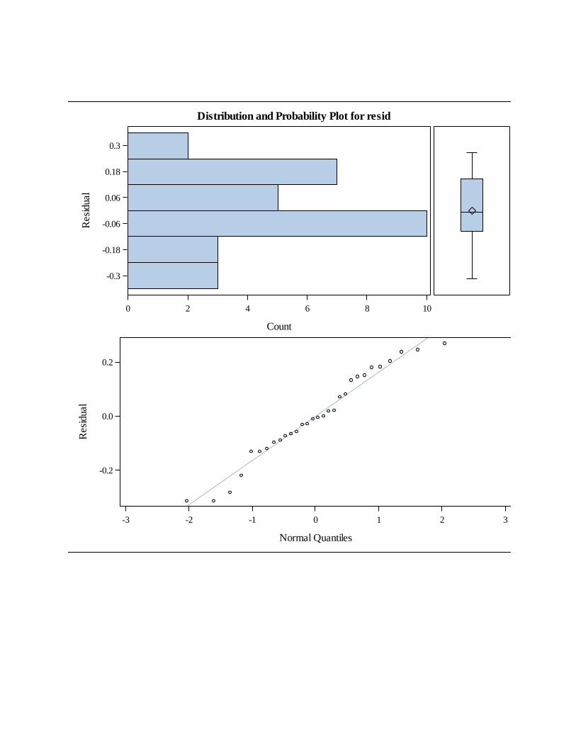
Figure 12: Distribution and Probability Plot of the Residuals

We next look at the histogram and box plot of the residuals to check for normality. We

can see that both are approximately normal. The points on the normal quartiles chart should form

a linear shape. The points do form roughly a linear shape in the graph above.

Distribution and Probability Plot for resid

-3 -2 -1 0 1 2 3

Normal Quantiles

-0.2

0.0

0.2

Resi

dual

0 2 4 6 8 10

Count

-0.3

-0.18

-0.06

0.06

0.18

0.3

Resi

dual

32

CONCLUSION

The assumptions for the regression analysis held for this chlorine model. Based on the

data and analysis, there was a negative correlation between when a water sample is collected

later in the day and the total chlorine level. Overall, there is a positive correlation between a

water sample’s temperature and the total chlorine level. There is a negative correlation between a

water sample’s storage time and the total chlorine level. The western region contains, on

average, the least amount of chlorine in comparison to the eastern and northern regions. The

northern region contains higher chlorine levels than the western and eastern regions. Further

analysis on the data must be done in order to establish a possible cause and effect relationship

between the independent and dependent variables. There was no testing of the interaction of the

independent variables, which could help to explain some of the counter intuitive results.

33

FUTURE RESEARCH

A nonparametric regression analysis can be performed for further research of the existing

data. A nonparametric analysis is appropriate if the data contains outlier that may be inaccurate,

but there is insufficient evidence to remove the data points. The parametric and nonparametric

regressions will be compared with each other to see which is a better predictor of the chlorine

level. “…seasonal changes in temperature (as well seasonal changes in precipitation) can

contribute to the variability in municipal drinking water quality.” (Dyck) Data can be collected

throughout the year, for a total of 12 months. By doing so, one can observe any seasonal

relationship between the season and the chlorine level. Due to seasonal changes in temperature

and precipitation the levels of chlorine in the water could also be affected. This change is worth

investigating to see if it is significant in the regression model for predicting the chlorine levels.

Water systems try to maintain an effect chlorine level throughout the entire water system. “This

requires a much higher concentration of chlorine at entry than the concentration that is to be

achieved at the extremities,” (Fisher) There can be a measureable difference in chlorine levels

between water samples collected near the water treatment plants and those further away. This

could lead to the addition of a distance variable to account for a water sample’s location in

comparison to the water treatment plant. By contacting the water treatment plants the estimated

water age of the samples can be collected and used to see if it is influential in predicting the

levels of chlorine. The interaction between the different independent variables should be

investigated in order to see if these interactions lead to a better understanding of how they affect

the chlorine levels. From the correlation matrix, one can see that adding an interaction between

the storage time and the time of day or possibly the storage time and the temperature of the water

34

sample. One could also test to see if there is a significant difference between the three different

treatment areas. If there is a significant difference, one can look at each treatment area separately

and see if this changes how the independent variables are affecting the total chlorine.

35

APPENDIX A: DATA

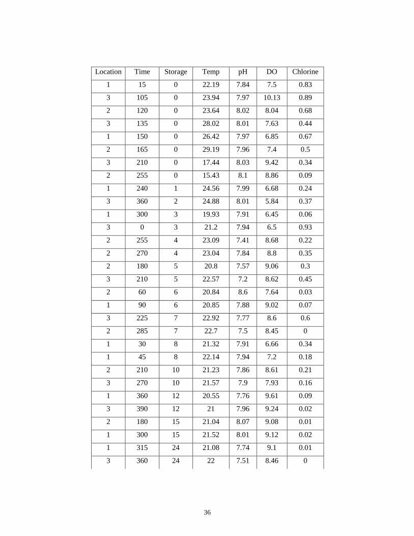
36

Location Time Storage Temp pH DO Chlorine

1 15 0 22.19 7.84 7.5 0.83

3 105 0 23.94 7.97 10.13 0.89

2 120 0 23.64 8.02 8.04 0.68

3 135 0 28.02 8.01 7.63 0.44

1 150 0 26.42 7.97 6.85 0.67

2 165 0 29.19 7.96 7.4 0.5

3 210 0 17.44 8.03 9.42 0.34

2 255 0 15.43 8.1 8.86 0.09

1 240 1 24.56 7.99 6.68 0.24

3 360 2 24.88 8.01 5.84 0.37

1 300 3 19.93 7.91 6.45 0.06

3 0 3 21.2 7.94 6.5 0.93

2 255 4 23.09 7.41 8.68 0.22

2 270 4 23.04 7.84 8.8 0.35

2 180 5 20.8 7.57 9.06 0.3

3 210 5 22.57 7.2 8.62 0.45

2 60 6 20.84 8.6 7.64 0.03

1 90 6 20.85 7.88 9.02 0.07

3 225 7 22.92 7.77 8.6 0.6

2 285 7 22.7 7.5 8.45 0

1 30 8 21.32 7.91 6.66 0.34

1 45 8 22.14 7.94 7.2 0.18

2 210 10 21.23 7.86 8.61 0.21

3 270 10 21.57 7.9 7.93 0.16

1 360 12 20.55 7.76 9.61 0.09

3 390 12 21 7.96 9.24 0.02

2 180 15 21.04 8.07 9.08 0.01

1 300 15 21.52 8.01 9.12 0.02

1 315 24 21.08 7.74 9.1 0.01

3 360 24 22 7.51 8.46 0

37

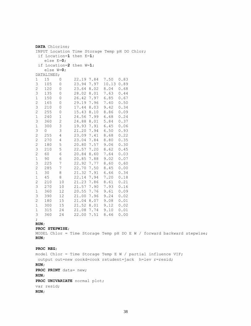
APPENDIX B: SAS CODE

38

DATA Chlorine;

INPUT Location Time Storage Temp pH DO Chlor;

if Location=1 then E=1;

else E=0;

if Location=2 then W=1;

else W=0;

DATALINES;

1 15 0 22.19 7.84 7.50 0.83

3 105 0 23.94 7.97 10.13 0.89

2 120 0 23.64 8.02 8.04 0.68

3 135 0 28.02 8.01 7.63 0.44

1 150 0 26.42 7.97 6.85 0.67

2 165 0 29.19 7.96 7.40 0.50

3 210 0 17.44 8.03 9.42 0.34

2 255 0 15.43 8.10 8.86 0.09

1 240 1 24.56 7.99 6.68 0.24

3 360 2 24.88 8.01 5.84 0.37

1 300 3 19.93 7.91 6.45 0.06

3 0 3 21.20 7.94 6.50 0.93

2 255 4 23.09 7.41 8.68 0.22

2 270 4 23.04 7.84 8.80 0.35

2 180 5 20.80 7.57 9.06 0.30

3 210 5 22.57 7.20 8.62 0.45

2 60 6 20.84 8.60 7.64 0.03

1 90 6 20.85 7.88 9.02 0.07

3 225 7 22.92 7.77 8.60 0.60

2 285 7 22.70 7.50 8.45 0.00

1 30 8 21.32 7.91 6.66 0.34

1 45 8 22.14 7.94 7.20 0.18

2 210 10 21.23 7.86 8.61 0.21

3 270 10 21.57 7.90 7.93 0.16

1 360 12 20.55 7.76 9.61 0.09

3 390 12 21.00 7.96 9.24 0.02

2 180 15 21.04 8.07 9.08 0.01

1 300 15 21.52 8.01 9.12 0.02

1 315 24 21.08 7.74 9.10 0.01

3 360 24 22.00 7.51 8.46 0.00

;

RUN;

PROC STEPWISE;

MODEL Chlor = Time Storage Temp pH DO E W / forward backward stepwise;

RUN;

PROC REG;

model Chlor = Time Storage Temp E W / partial influence VIF;

output out=new cookd=cook rstudent=jack h=lev r=resid;

RUN;

PROC PRINT data= new;

RUN;

PROC UNIVARIATE normal plot;

var resid;

RUN;

39

PROC CORR;

var Time Storage Temp E W;

RUN;

40

APPENDIX C: SAS OUTPUT

41

Number of Observations Read

30

Number of Observations Used

30

Forward Selection: Step 1

Variable Storage Entered: R-Square = 0.3743 and C(p) = 19.3482


Source DF Sum of

Squares Mean

Square F Value Pr > F

Model 1 0.86768 0.86768 16.75 0.0003

Error 28 1.45058 0.05181

Corrected Total

29 2.31827

Variable Parameter

Estimate Standard

Error Type II SS F

Value Pr > F

Intercept 0.46929 0.05806 3.38428 65.33 <.0001

Storage -0.02607 0.00637 0.86768 16.75 0.0003

Bounds on condition number: 1,

1

The SAS System

The STEPWISE Procedure

Model: MODEL1 Dependent Variable:

Chlor



Variable Time Entered: R-Square = 0.4846 and C(p) = 13.3516


Source DF Sum of

Squares Mean


Model 2 1.12348 0.56174 12.69 0.0001

Error 27 1.19479 0.04425

Corrected Total

29 2.31827

Variable Parameter

Estimate Standard

Error Type II SS F

Value Pr > F

Intercept 0.61713 0.08161 2.53024 57.18 <.0001

Time -0.00094707 0.00039392 0.25579 5.78 0.0233

Storage -0.01909 0.00656 0.37440 8.46 0.0072

Bounds on condition number: 1.243,

4.972


The SAS System



Chlor


Variable Temp Entered: R-Square = 0.5506 and C(p) = 10.5676


Source DF Sum of

Squares Mean


Model 3 1.27651 0.42550 10.62 <.0001

Error 26 1.04176 0.04007

Corrected Total

29 2.31827

Variable Parameter

Estimate Standard

Error Type II SS

F Valu

e Pr > F

Intercept -0.02330 0.33678 0.00019172 0.00 0.9454

Time -0.00093528 0.00037488 0.24940 6.22 0.0193

Storage -0.01629 0.00641 0.25910 6.47 0.0173

Temp 0.02789 0.01427 0.15303 3.82 0.0615


10.864


The SAS System



Chlor


Variable W Entered: R-Square = 0.5995 and C(p) = 9.0232


Source DF Sum of

Squares Mean


Model 4 1.38988 0.34747 9.36 <.0001

Error 25 0.92838 0.03714

Corrected Total

29 2.31827

The SAS System



Chlor


Variable Parameter

Estimate Standard

Error Type II S

S F Value Pr > F

Intercept 0.06693 0.32830 0.00154 0.04 0.8401

Time -0.00091597 0.00036107 0.23898 6.44 0.0178

Storage -0.01793 0.00624 0.30671 8.26 0.0082

Temp 0.02611 0.01378 0.13333 3.59 0.0697

W -0.13208 0.07559 0.11338 3.05 0.0929


18.738


Variable E Entered: R-Square = 0.6653 and C(p) = 6.2559

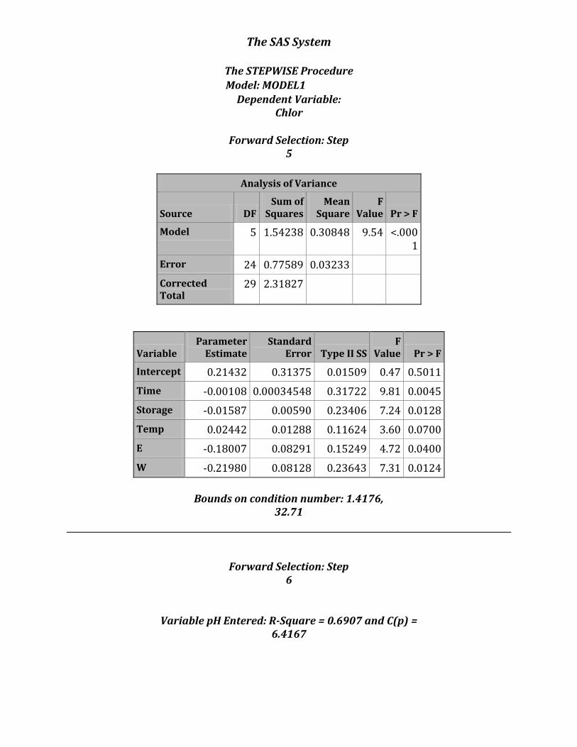
The SAS System



Chlor



Source DF Sum of

Squares Mean

Square F

Value Pr > F

Model 5 1.54238 0.30848 9.54 <.0001

Error 24 0.77589 0.03233

Corrected Total

29 2.31827

Variable Parameter

Estimate Standard

Error Type II SS F

Value Pr > F

Intercept 0.21432 0.31375 0.01509 0.47 0.5011

Time -0.00108 0.00034548 0.31722 9.81 0.0045

Storage -0.01587 0.00590 0.23406 7.24 0.0128

Temp 0.02442 0.01288 0.11624 3.60 0.0700

E -0.18007 0.08291 0.15249 4.72 0.0400

W -0.21980 0.08128 0.23643 7.31 0.0124


32.71


Variable pH Entered: R-Square = 0.6907 and C(p) = 6.4167

The SAS System



Chlor



Source DF Sum of

Squares Mean

Square F

Value Pr > F

Model 6 1.60121 0.26687 8.56 <.0001

Error 23 0.71706 0.03118

Corrected Total

29 2.31827

Variable Parameter

Estimate Standard

Error Type II SS F

Value Pr > F

Intercept 1.78620 1.18499 0.07084 2.27 0.1453

Time -0.00118 0.00034734 0.36256 11.63 0.0024

Storage -0.01705 0.00586 0.26433 8.48 0.0079

Temp 0.02220 0.01275 0.09451 3.03 0.0950

pH -0.19045 0.13863 0.05883 1.89 0.1828

E -0.17145 0.08166 0.13741 4.41 0.0470

W -0.21314 0.07996 0.22151 7.10 0.0138


46.86

No other variable met the 0.5000 significance level for entry into the model.

The SAS System



Chlor

Summary of Forward Selection


Number Vars In

Partial R-Square

Model R-Square C(p)

F Value Pr > F

1 Storage 1 0.3743 0.3743 19.3482 16.75 0.0003

2 Time 2 0.1103 0.4846 13.3516 5.78 0.0233

3 Temp 3 0.0660 0.5506 10.5676 3.82 0.0615

4 W 4 0.0489 0.5995 9.0232 3.05 0.0929

5 E 5 0.0658 0.6653 6.2559 4.72 0.0400

6 pH 6 0.0254 0.6907 6.4167 1.89 0.1828

The SAS System



Chlor


30


30

Backward Elimination: Step 0

All Variables Entered: R-Square = 0.6964 and C(p) = 8.0000


Source DF Sum of

Squares Mean

Square

F Valu

e Pr > F

Model 7 1.61454 0.23065 7.21 0.0002

Error 22 0.70373 0.03199

Corrected Total

29 2.31827

The SAS System



Chlor


Variable Parameter

Estimate Standard

Error Type II

SS F Value Pr > F

Intercept 1.39297 1.34605 0.03426 1.07 0.3120

Time -0.00120 0.00035268 0.37048 11.58 0.0026

Storage -0.01796 0.00610 0.27760 8.68 0.0075

Temp 0.02521 0.01373 0.10783 3.37 0.0799

pH -0.17275 0.14308 0.04663 1.46 0.2401

DO 0.02380 0.03688 0.01333 0.42 0.5253

E -0.16053 0.08443 0.11563 3.61 0.0704

W -0.21979 0.08165 0.23180 7.25 0.0133


67.472


Variable DO Removed: R-Square = 0.6907 and C(p) = 6.4167

The SAS System



Chlor



Source DF Sum of

Squares Mean

Square

F Valu

e Pr > F

Model 6 1.60121 0.26687 8.56 <.0001

Error 23 0.71706 0.03118

Corrected Total

29 2.31827

Variable Parameter

Estimate Standard

Error Type II S

S F

Value Pr > F

Intercept 1.78620 1.18499 0.07084 2.27 0.1453

Time -0.00118 0.00034734 0.36256 11.63 0.0024

Storage -0.01705 0.00586 0.26433 8.48 0.0079

Temp 0.02220 0.01275 0.09451 3.03 0.0950

pH -0.19045 0.13863 0.05883 1.89 0.1828

E -0.17145 0.08166 0.13741 4.41 0.0470

W -0.21314 0.07996 0.22151 7.10 0.0138


46.86


Variable pH Removed: R-Square = 0.6653 and C(p) = 6.2559

The SAS System



Chlor



Source DF Sum of

Squares Mean

Square F

Value Pr > F

Model 5 1.54238 0.30848 9.54 <.0001

Error 24 0.77589 0.03233

Corrected Total

29 2.31827

Variable Parameter

Estimate Standard

Error Type II SS F

Value Pr > F

Intercept 0.21432 0.31375 0.01509 0.47 0.5011

Time -0.00108 0.00034548 0.31722 9.81 0.0045

Storage -0.01587 0.00590 0.23406 7.24 0.0128

Temp 0.02442 0.01288 0.11624 3.60 0.0700

E -0.18007 0.08291 0.15249 4.72 0.0400

W -0.21980 0.08128 0.23643 7.31 0.0124


32.71

All variables left in the model are significant at the 0.1000 level.

The SAS System



Chlor

Summary of Backward Elimination

Step Variable Removed

Number Vars In

Partial R-

Square

Model R-

Square C(p) F

Value Pr > F

1 DO 6 0.0057 0.6907 6.4167 0.42 0.5253

2 pH 5 0.0254 0.6653 6.2559 1.89 0.1828

The SAS System



Chlor


30


30

Stepwise Selection: Step 1

Variable Storage Entered: R-Square = 0.3743 and C(p) = 19.3482


Source DF Sum of

Squares Mean

Square F

Value Pr > F

Model 1 0.86768 0.86768 16.75 0.0003

Error 28 1.45058 0.05181

Corrected Total

29 2.31827

Variable Parameter

Estimate Standard

Error Type II SS F Value Pr > F

Intercept 0.46929 0.05806 3.38428 65.33 <.0001

Storage -0.02607 0.00637 0.86768 16.75 0.0003

Bounds on condition number: 1,

1

The SAS System



Chlor


04:37 Friday, December 04, 2015 55

Stepwise Selection: Step

2

Variable Time Entered: R-Square = 0.4846 and C(p) = 13.3516


Source DF Sum of

Squares Mean

Square F

Value Pr > F

Model 2 1.12348 0.56174 12.69 0.0001

Error 27 1.19479 0.04425

Corrected Total

29 2.31827

Variable Parameter

Estimate Standard

Error Type II SS F

Value Pr > F

Intercept 0.61713 0.08161 2.53024 57.18 <.0001

Time -0.00094707 0.00039392 0.25579 5.78 0.0233

Storage -0.01909 0.00656 0.37440 8.46 0.0072


4.972

The SAS System



Chlor



Variable Temp Entered: R-Square = 0.5506 and C(p) = 10.5676


Source DF Sum of

Squares Mean

Square F

Value Pr > F

Model 3 1.27651 0.42550 10.62 <.0001

Error 26 1.04176 0.04007

Corrected Total

29 2.31827

Variable Parameter

Estimate Standard

Error Type II SS F

Value Pr > F

Intercept -0.02330 0.33678 0.00019172 0.00 0.9454

Time -0.00093528 0.00037488 0.24940 6.22 0.0193

Storage -0.01629 0.00641 0.25910 6.47 0.0173

Temp 0.02789 0.01427 0.15303 3.82 0.0615


10.864

The SAS System



Chlor



Variable W Entered: R-Square = 0.5995 and C(p) = 9.0232


Source DF Sum of

Squares Mean

Square F

Value Pr > F

Model 4 1.38988 0.34747 9.36 <.0001

Error 25 0.92838 0.03714

Corrected Total

29 2.31827

Variable Parameter

Estimate Standard

Error Type II SS F

Value Pr > F

Intercept 0.06693 0.32830 0.00154 0.04 0.8401

Time -0.00091597 0.00036107 0.23898 6.44 0.0178

Storage -0.01793 0.00624 0.30671 8.26 0.0082

Temp 0.02611 0.01378 0.13333 3.59 0.0697

W -0.13208 0.07559 0.11338 3.05 0.0929


18.738

The SAS System



Chlor



Variable E Entered: R-Square = 0.6653 and C(p) = 6.2559


Source DF Sum of

Squares Mean

Square F

Value Pr > F

Model 5 1.54238 0.30848 9.54 <.0001

Error 24 0.77589 0.03233

Corrected Total

29 2.31827

Variable Parameter

Estimate Standard

Error Type II SS F

Value Pr > F

Intercept 0.21432 0.31375 0.01509 0.47 0.5011

Time -0.00108 0.00034548 0.31722 9.81 0.0045

Storage -0.01587 0.00590 0.23406 7.24 0.0128

Temp 0.02442 0.01288 0.11624 3.60 0.0700

E -0.18007 0.08291 0.15249 4.72 0.0400

W -0.21980 0.08128 0.23643 7.31 0.0124


32.71

The SAS System



Chlor


All variables left in the model are significant at the 0.1500 level.

No other variable met the 0.1500 significance level for entry into the

model.

Summary of Stepwise Selection


Variable Removed

Number Vars In

Partial R-Square

Model R-Square C(p)

F Value Pr > F

1 Storage 1 0.3743 0.3743 19.3482 16.75 0.0003

2 Time 2 0.1103 0.4846 13.3516 5.78 0.0233

3 Temp 3 0.0660 0.5506 10.5676 3.82 0.0615

4 W 4 0.0489 0.5995 9.0232 3.05 0.0929

5 E 5 0.0658 0.6653 6.2559 4.72 0.0400

The SAS System

The REG Procedure


Chlor


30


30


Source DF Sum of

Squares Mean

Square F

Value Pr > F

Model 5 1.54238 0.30848 9.54 <.0001

Error 24 0.77589 0.03233

Corrected Total

29 2.31827

Root MSE 0.17980 R-Square

0.6653

Dependent Mean

0.30333 Adj R-Sq 0.5956

Coeff Var 59.27542

Parameter Estimates

Variable DF Parameter

Estimate Standard

Error t Value Pr > |t| Variance Inflation

Intercept 1 0.21432 0.31375 0.68 0.5011 0

Time 1 -0.00108 0.00034548 -3.13 0.0045 1.30872

Storage 1 -0.01587 0.00590 -2.69 0.0128 1.37402

Temp 1 0.02442 0.01288 1.90 0.0700 1.07951

E 1 -0.18007 0.08291 -2.17 0.0400 1.41762

W 1 -0.21980 0.08128 -2.70 0.0124 1.36223

The SAS System

The REG Procedure


Chlor

Output Statistics

Obs Residual RStudent Hat Diag

H

Cov Rati

o DFFITS

DFBETAS

Intercept Time

Storage Temp E W

1 0.2701 1.7444 0.1953 0.7612

0.8593 0.2250 -0.413

5

-0.2043

-0.105

5

0.3615

-0.075

5

2 0.2047 1.2521 0.1538 1.0271

0.5338 0.0777 -0.188

6

-0.1099

0.0652

-0.312

2

-0.328

8

3 0.2380 1.4530 0.1313 0.8774

0.5648 -0.0585 -0.112

6

-0.1189

0.1088

0.0006

0.3287

4 -0.3125 -2.1630 0.2555 0.5709

-1.2669 0.5910 0.1832

0.1071 -0.856

5

0.4987

0.5244

5 0.1529 0.9584 0.2154 1.3008

0.5021 -0.2511 0.0593

-0.1674

0.2766

0.2831

0.0125

6 -0.0288 -0.1933 0.3416 1.9418

-0.1393 0.1043 -0.005

9

0.0067 -0.111

9

-0.010

4

-0.060

9

7 -0.0729 -0.4790 0.3057 1.7518

-0.3179 -0.2636 -0.029

2

0.1566 0.2370

0.1223

0.1543

8 -0.00536

6

-0.0383 0.4167 2.2122

-0.0323 -0.0235 -0.008

6

0.0161 0.0256

-0.001

1

-0.008

9

9 -0.1184 -0.7275 0.1966 1.4018

-0.3599 0.1214 -0.170

1

0.1853 -0.109

0

-0.232

7

-0.012

3

10 -0.0306 -0.1908 0.2378 1.6777

-0.1066 0.0283 -0.070

8

0.0479 -0.031

2

0.0278

0.0417

The SAS System

The REG Procedure


Chlor

Output Statistics


H

Cov Rati

o DFFITS

DFBETAS

Intercept Time

Storage Temp E W

11 -0.0887 -0.5558 0.2352 1.5581

-0.3082 -0.0820 -0.182

2

0.1821 0.1144

-0.179

0

0.0020

12 0.2456 1.6623 0.2753 0.9018

1.0246 0.5257 -0.760

5

0.1267 -0.258

3

-0.589

1

-0.531

7

13 0.001053

0.006115

0.1212 1.4689

0.0023 -0.0006 0.0008

-0.0005

0.0004

0.0002

0.0015

14 0.1485 0.8808 0.1289 1.2144

0.3388 -0.0827 0.1475

-0.0785

0.0596

0.0382

0.2241

15 0.0717 0.4152 0.1101 1.3870

0.1460 0.0430 -0.015

7

-0.0036

-0.041

7

-0.005

6

0.0922

16 -0.00887

8

-0.0510 0.1016 1.4359

-0.0171 -0.0039 0.0007

0.0015 0.0005

0.0117

0.0122

17 -0.3133 -2.0579 0.1864 0.5756

-0.9851 -0.3171 0.6405

-0.2925

0.2074

0.1573

-0.437

7

18 -0.2808 -1.7526 0.1374 0.7055

-0.6996 -0.2541 0.3000

-0.0122

0.1951

-0.340

4

0.0493

19 0.1805 1.0622 0.1015 1.0780

0.3571 0.0314 -0.013

9

0.0336 0.0349

-0.246

1

-0.244

2

20 -0.1293 -0.7627 0.1259 1.2713

-0.2895 0.0744 -0.114

6

0.0024 -0.049

8

-0.024

1

-0.197

7

21 -0.0555 -0.3373 0.1942 1.5554

-0.1656 -0.0429 0.1137

-0.0492

0.0220

-0.055

0

0.0111

The SAS System

The REG Procedure


Chlor

Output Statistics


H

Cov Rati

o DFFITS

DFBETAS

Intercept Time

Storage Temp E W

22 -0.2193 -1.3660 0.1743 0.9791

-0.6275 -0.0774 0.4093

-0.1967

-0.001

5

-0.234

9

0.0323

23 0.0830 0.4848 0.1225 1.3841

0.1811 0.0109 -0.026

1

0.0708 -0.013

8

-0.012

7

0.1165

24 -0.1302 -0.7622 0.1136 1.2539

-0.2728 -0.0656 -0.022

3

-0.0556

0.0338

0.1798

0.1740

25 0.1339 0.8243 0.1942 1.3452

0.4046 -0.0007 0.2492

-0.0304

-0.062

5

0.2409

0.0230

26 -0.0947 -0.5741 0.1826 1.4501

-0.2714 -0.0351 -0.144

6

-0.0142

0.0394

0.1169

0.1246

27 -0.0655 -0.4030 0.2118 1.5702

-0.2089 -0.0057 0.0824

-0.1469

0.0027

0.0293

-0.103

0

28 0.0229 0.1360 0.1561 1.5224

0.0585 -0.0092 0.0169

0.0195 0.0029

0.0333

0.0040

29 0.1827 1.2434 0.3167 1.2787

0.8464 -0.1509 0.0153

0.6129 0.0805

0.2740

0.0610

30 0.0189 0.1287 0.3609 2.0111

0.0967 -0.0133 -0.000

6

0.0737 0.0151

-0.041

2

-0.028

2

The SAS System

The REG Procedure


Chlor

Sum of Residuals 0

Sum of Squared Residuals 0.77589

Predicted Residual SS (PRESS)

1.20403

The SAS System

The REG Procedure

Model: MODEL1

Fit Diagnostics for Chlor

0.5956Adj R-Square

0.6653R-Square

0.0323MSE

24Error DF

6Parameters

30Observations

Proportion Less

0.0 0.4 0.8

Residual

0.0 0.4 0.8

Fit–Mean

-0.4

-0.2

0.0

0.2

0.4

-0.54 -0.18 0.18 0.54

Residual

0

10

20

30

Perc

en

t

0 5 10 15 20 25 30

Observation

0.00

0.05

0.10

0.15

0.20

Co

ok's

D

-0.2 0.0 0.2 0.4 0.6 0.8

Predicted Value

-0.2

0.0

0.2

0.4

0.6

0.8

Ch

lor

-2 -1 0 1 2

Quantile

-0.2

0.0

0.2

Resid

ual

0.1 0.2 0.3 0.4

Leverage

-2

-1

0

1

2

RS

tud

en

t

-0.2 0.0 0.2 0.4 0.6 0.8

Predicted Value

-2

-1

0

1

2

RS

tud

en

t

-0.2 0.0 0.2 0.4 0.6 0.8

Predicted Value

-0.2

0.0

0.2

Resid

ual

The SAS System

The REG Procedure

Model: MODEL1

Residual by Regressors for Chlor

0.0 0.2 0.4 0.6 0.8 1.0

W

0.0 0.2 0.4 0.6 0.8 1.0

E

15.0 17.5 20.0 22.5 25.0 27.5

Temp

0 5 10 15 20 25

Storage

0 100 200 300 400

Time

-0.2

0.0

0.2

Resid

ual

-0.2

0.0

0.2

Resid

ual

The SAS System

The REG Procedure

Model: MODEL1 Partial Regression Residual

Plot

Partial Plots for Chlor

Partial Regressor Residual

Part

ial D

ependent

Resi

dual

-0.50 -0.25 0.00 0.25 0.50

-0.4

-0.2

0.0

0.2

0.4

W

-0.5 0.0 0.5

-0.4

-0.2

0.0

0.2

0.4

E

-5 0 5

-0.4

-0.2

0.0

0.2

Temp

-10 -5 0 5 10 15

-0.4

-0.2

0.0

0.2

Storage

-200 -100 0 100

-0.2

0.0

0.2

0.4

Time

-0.2 -0.1 0.0 0.1 0.2

-0.4

-0.2

0.0

0.2

Intercept

The SAS System


1 1 15 0 22.19 7.84 7.50 0.83 1 0 0.27010 0.11341 0.19528 1.74439

2 3 105 0 23.94 7.97 10.13 0.89 0 0 0.20469 0.04639 0.15379 1.25208

3 2 120 0 23.64 8.02 8.04 0.68 0 1 0.23805 0.05082 0.13129 1.45296

4 3 135 0 28.02 8.01 7.63 0.44 0 0 -0.31248 0.23197 0.25545 -2.16296

5 1 150 0 26.42 7.97 6.85 0.67 1 0 0.15290 0.04216 0.21537 0.95837

6 2 165 0 29.19 7.96 7.40 0.50 0 1 -0.02879 0.00337 0.34162 -0.19333

7 3 210 0 17.44 8.03 9.42 0.34 0 0 -0.07295 0.01740 0.30570 -0.47904

8 2 255 0 15.43 8.10 8.86 0.09 0 1 -0.00537 0.00018 0.41668 -0.03825

9 1 240 1 24.56 7.99 6.68 0.24 1 0 -0.11841 0.02202 0.19659 -0.72750

10 3 360 2 24.88 8.01 5.84 0.37 0 0 -0.03057 0.00197 0.23779 -0.19078

11 1 300 3 19.93 7.91 6.45 0.06 1 0 -0.08868 0.01630 0.23520 -0.55576

12 3 0 3 21.20 7.94 6.50 0.93 0 0 0.24558 0.16298 0.27530 1.66230

13 2 255 4 23.09 7.41 8.68 0.22 0 1 0.00105 0.00000 0.12115 0.00611

14 2 270 4 23.04 7.84 8.80 0.35 0 1 0.14851 0.01931 0.12887 0.88079

15 2 180 5 20.80 7.57 9.06 0.30 0 1 0.07168 0.00368 0.11008 0.41525

16 3 210 5 22.57 7.20 8.62 0.45 0 0 -0.00888 0.00005 0.10159 -0.05100

17 2 60 6 20.84 8.60 7.64 0.03 0 1 -0.31329 0.14253 0.18643 -2.05785

18 1 90 6 20.85 7.88 9.02 0.07 1 0 -0.28080 0.07509 0.13744 -1.75259

19 3 225 7 22.92 7.77 8.60 0.60 0 0 0.18055 0.02114 0.10154 1.06220

20 2 285 7 22.70 7.50 8.45 0.00 0 1 -0.12935 0.01422 0.12593 -0.76274

21 1 30 8 21.32 7.91 6.66 0.34 1 0 -0.05547 0.00474 0.19422 -0.33725

22 1 45 8 22.14 7.94 7.20 0.18 1 0 -0.21926 0.06335 0.17427 -1.36596

23 2 210 10 21.23 7.86 8.61 0.21 0 1 0.08299 0.00565 0.12249 0.48483

24 3 270 10 21.57 7.90 7.93 0.16 0 0 -0.13018 0.01263 0.11358 -0.76224

25 1 360 12 20.55 7.76 9.61 0.09 1 0 0.13394 0.02766 0.19418 0.82430

26 3 390 12 21.00 7.96 9.24 0.02 0 0 -0.09465 0.01263 0.18263 -0.57409

27 2 180 15 21.04 8.07 9.08 0.01 0 1 -0.06548 0.00754 0.21183 -0.40301

28 1 300 15 21.52 8.01 9.12 0.02 1 0 0.02293 0.00059 0.15614 0.13597

29 1 315 24 21.08 7.74 9.10 0.01 1 0 0.18274 0.11675 0.31667 1.24337

30 3 360 24 22.00 7.51 8.46 0.00 0 0 0.01890 0.00163 0.36088 0.12873

The SAS System

The UNIVARIATE Procedure

Variable: resid (Residual)

Moments

N 30 Sum Weights 30

Mean 0 Sum Observations

0

Std Deviation

0.16356914 Variance 0.02675486

Skewness -0.1995171 Kurtosis -0.5999978

Uncorrected SS

0.77589104 Corrected SS 0.77589104

Coeff Variation

. Std Error Mean

0.0298635

Basic Statistical Measures

Location Variability

Mean 0.00000 Std Deviation 0.16357

Median -0.00712 Variance 0.02675

Mode . Range 0.58339

Interquartile Range

0.24316

Tests for Location: Mu0=0


Student's t t 0 Pr > |t| 1.0000

Sign M -1 Pr >= |M|

0.8555

Signed Rank

S 0.5 Pr >= |S| 0.9920

The SAS System



Tests for Normality


Shapiro-Wilk W 0.963015 Pr < W 0.3690

Kolmogorov-Smirnov

D 0.093572 Pr > D >0.1500

Cramer-von Mises W-Sq 0.038275 Pr > W-Sq >0.2500

Anderson-Darling A-Sq 0.301686 Pr > A-Sq >0.2500

Quantiles (Definition 5)

Level Quantile

100% Max 0.27009815

99% 0.27009815

95% 0.24557640

90% 0.22136644

75% Q3 0.14850690

50% Median

-0.00712177

25% Q1 -0.09465376

10% -0.25002667

5% -0.31248174

1% -0.31329171

0% Min -0.31329171

Extreme Observations

Lowest Highest

Value Obs Value Obs

-0.313292 17 0.182737 29

-0.312482 4 0.204687 2

-0.280796 18 0.238046 3

The SAS System



Extreme Observations

Lowest Highest

Value Obs Value Obs

-0.219258 22 0.245576 12

-0.130177 24 0.270098 1

Distribution and Probability Plot for resid

-3 -2 -1 0 1 2 3

Normal Quantiles

-0.2

0.0

0.2

Resi

dual

0 2 4 6 8 10

Count

-0.3

-0.18

-0.06

0.06

0.18

0.3

Resi

dual

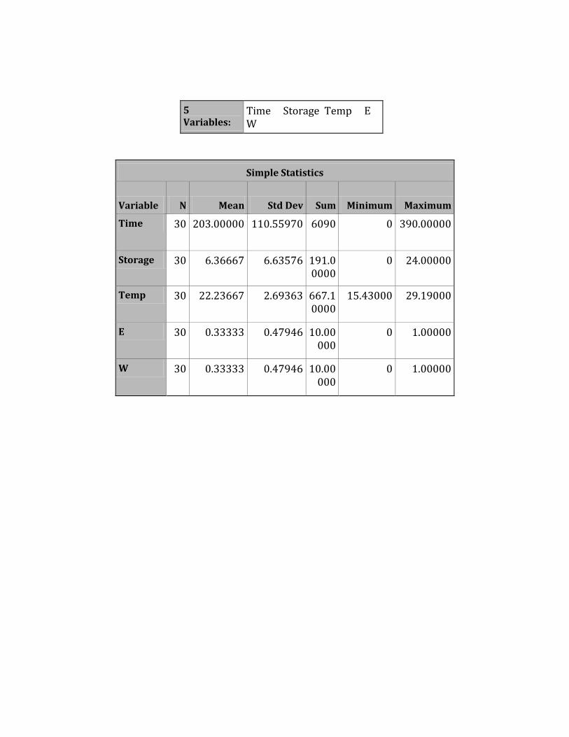
5 Variables:


Simple Statistics

Variable N Mean Std Dev Sum Minimum Maximum

Time 30 203.00000 110.55970 6090 0 390.00000

Storage 30 6.36667 6.63576 191.00000

0 24.00000

Temp 30 22.23667 2.69363 667.10000

15.43000 29.19000

E 30 0.33333 0.47946 10.00000

0 1.00000

W 30 0.33333 0.47946 10.00000

0 1.00000

Pearson Correlation Coefficients, N = 30 Prob > |r| under H0: Rho=0


Time 1.00000

0.44215 0.0144

-0.12659 0.5050

-0.12034 0.5264

-0.03253 0.8645

Storage 0.44215 0.0144

1.00000

-0.25474 0.1743

0.14451 0.4461

-0.13728 0.4694

Temp -0.12659 0.5050

-0.25474 0.1743

1.00000

-0.04824 0.8002

-0.03649 0.8482

E -0.12034 0.5264

0.14451 0.4461

-0.04824 0.8002

1.00000

-0.50000 0.0049

W -0.03253 0.8645

-0.13728 0.4694

-0.03649 0.8482

-0.50000 0.0049

1.00000

REFERENCES

Ali, Aftab, Malgorzata Kurzawa-Zegota, Mojgan Najafzadeh, Rajendran C. Gopalan, Michael J.

Plewa, and Diana Anderson. "Effect of Drinking Water Disinfection By-products in

Human Peripheral Blood Lymphocytes and Sperm." Mutation Research/Fundamental and

Molecular Mechanisms of Mutagenesis 770 (2014): 136-43. Web. 15 Mar. 2015.

Dyck, Roberta, Geneviève Cool, Manuel Rodriguez, and Rehan Sadiq. "Treatment, Residual

Chlorine and Season as Factors Affecting Variability of Trihalomethanes in Small Drinking

Water Systems." Frontiers of Environmental Science & Engineering 9.1 (2015): 171-79.

Print.

Fisher, Ian, George Kastl, and Arumugam Sathasivan. "A Suitable Model of Combined Effects of

Temperature and Initial Condition on Chlorine Bulk Decay in Water Distribution

Systems." Water Research 46.10 (2010): 3293-303. Web. 5 Mar. 2015.

"Free Chlorine Testing." Centers for Disease Control and Prevention. Centers for Disease Control

and Prevention, 17 July 2014. Web. 20 Mar. 2015.

Liu, Boning, David A. Reckhow, and Yun Li. "A Two-site Chlorine Decay Model for the

Combined Effects of PH, Water Distribution Temperature and In-home Heating Profiles

Using Differential Evolution." Water Research 53 (2014): 47-57. Web. 10 Mar. 2015.

Lyon, Bonnie. "Integrated Chemical and Toxicological Investigation of UV-Chlorine/

Chloramine Drinking Water Treatment." Environmental Science & Technology 48.12

(2014): 6743-753. Print.

Sorlini, Sabrina, Francesca Gialdini, Michela Biasibetti, and Carlo Collivignarelli. "Influence of

Drinking Water Treatments on Chlorine Dioxide Consumption and Chlorite/chlorate

Formation."Water Research 54 (2014): 44-52. Web. 20 Mar. 2015.

Wang, Yifei, Aiyin Jia, Yue Wu, Chunde Wu, and Lijun Chen. "Disinfection of Bore Well

Water with Chlorine Dioxide/sodium Hypochlorite and Hydrodynamic

Cavitation." Enivironmental Technology 36.4 (2015): 479-86. Web. 20 Mar. 2015.

"Water Quality." Water Quality. N.p., n.d. Web. 29 Mar. 2015.

<http://www.orangecountyfl.net/Water,GarbageRecycling/WaterQuality.aspx#.VUD5BK3

BzGc>.

Waters, Brian W., and Yen-Con Hung. "The Effect of PH and Chloride Concentration on the

Stability and Antimicrobial Activity of Chlorine-Based Sanitizers." Journal of Food

Science 79 (2014): n. pag. Biological Abstracts [EBSCO]. Web. 13 Mar. 2015.

Weisberg, Sanford. Preface. Applied Linear Regression. 3rd ed. Hoboken: Wiley Series in

Probability and Statistics, 2005. N. pag. Print.

Zimoch, Izabela. "The Optimization of Chlorine Dose in Water Treatment Process in Order to

Reduce the Formation of Disinfection By-Products." Desalination and Water Treatment 52

(2014): 3719-724. Print.

Documents

To Hydrate or Chlorinate: A Regression Analysis of the