http://repository.osakafu-u.ac.jp/dspace/

   

Title Analysis of Dynamics in Cellular Neural Network

Author(s) Tsubata, Toshihide; Kawabata, Hiroaki; Takeda, Yoji

Editor(s)

CitationBulletin of University of Osaka Prefecture. Series A, Engineering and nat

ural sciences. 1994, 42(2), p.145-156

Issue Date 1994-03-31

URL http://hdl.handle.net/10466/8585

Rights

Bulletin of University of Osaka Prefecture 145 Vol.42, No.2, 1993, pp. 145-156.

Analysis of Dynamies in Cellular Neural Networks

Toshihide TsuBATA*, Hiroaki KAwABATA**,

and Yoji TAKEDA""

(Received October 30, 1993)

Cellular neural network (CNN) with an external oscillating input has complex oscillations such as chaos, quasi-periodicity and intermittency. It also shows a phenomenon of an attractor switching for the unsymmetric template. This paper describes these oscillations and phenomena when an amplitude of the external input is changed. These oscillations in the CNN may show a possibility of dy- namic information-processing system.

' 1. Introduction

In order to achive a human-like operating of information processing, many studies

have been made with the neural networks. Neural networks are parallel information

processing systems and "cellular neural networks" (CNN's) proposed by L.O.Chua and

L.Yang are one of themi)'2). A CNN is made up of regularly spaced clone circuit,

called cell, which connects with only its neighbors, and this neural network has a pos-

sibility for the applications such as image processing or pattern recognization system.

Connection weights between one cell and the others are described by a "cloning tem-

plate" which specifies the dynamic rule of the cellular neural network. Depending on

the values of cloning template and the initial state, the various steady state perform-

ances appeari)･2)･`)･5)･6). At present, studies about cellular neural networks have been

done from the point of view of 'applying its stable steady states, which arise when

the symmetric template is cho,sen. In the meanwhile, when an unsymmetric cloning

template is chosen, the dynarnics does not always show a complete stability and a

ehaotic oscillation arises. Although it is difficult to use the chaotic oscillation for

the information processing, the amount of information which is included in the time

series is grea:ter than tha't of the static states. The analysis for the chaotic phenome-

na included in the CNN is insufficient at the present time3).

In this paper, we exarnine the dynamics of the chaotic oscillations-included in the

cellular neural networks. It is recognized that a variety of oscillation forms, such as

periodicity, quasi-periodicity,' intermittency, chaos, and attractor switching (attractor

merging) can be included in the CNN for an unsymmetric cloning template when the

amplitude of a periodic external input is changed.

* Sharp Co. Ltd.

** Department of Electrical and Electronic Systems, College of Engineering.

146 Toshihide TsuBATA, Hiroaki KAwABATA and Yoji TAKEDA

2. Model equation

ln general, a cellular neural network is composed of an mxn matrix cell neurons in

which the governing equation of the ij-th cell neuron is given by the following differen-

tial equation:

beii -- -xii+A*crij+B*uij+I, (1) (1<i<m, 1<J'<n)

where xii and uii are the state variable and input of the ij-th cell neuron. Iii stand

for the threshold value. A and B are the matrices which corespond to the connection

weight coefficients, and they are called "temlates". A * yij and B * uij are the inter-

ference terms of the outputs and inputs from the neighbor ce11s. The convolution oper-

ator * is introduced to express the interference terms with compact forms.

A*yii

attn -r

ao.: -r

ar -r

+------

+-i----

... a-c e

-:---'" (Ze,e

--: ---' a,;e

---.

' .i--..

.-i-

a-n r : .(Zo, r

: .anr

*yij

a-n -EYFn i-r+･"+a-ny oYi-n i+"'+a--r. Ot-n j+r (2)

+ CZe,-(Yt i--r+ ' " +(Zo. oYii+ " ' + (Zo, ,iYt H-r

+a,; -EYi+n i-r+ ' " +a,: oYi+,: j+ " ' +a,: EYi+,; i+n

Output yii is given by the following function of state xij.

yi, -- S- (lx,,+11-lx,,-1l ). (3)

' As mentioned in introduction, we focus on the chaotic dynarnics included in CNN,

so here we deal with a simple, one-dimensional spaced, cellu!ar neurai network which

is composed of only two neurons in Fig. 13). The dynarnics is described as follows;

[ill =l-,i -O,] [:I] +[e JSI[;ll+[6 ?][g(`)1+[81 (4)

where p is the feedback connection weight of a cell's output, s is the connection

weight from the neighbor cell, and g(t) is the external periodic force. In this case,

the template is described as (s, p, -s). The external input g(t) and the output func-

tion f(x)is described as follows;

g(t)= A. sin(2ztlT) (s) f( xi)=),i= S'(1 an+ 1l -lan" 1l ). (6)

Where A. is the amplitude and T is a period of the external input.

Analysis of Dynamics in Cellular Neural Nletworfes 147

s Yl

p Xl X2 p

so

9(t) -S Fig. 1 Simple model of CNN with an external input

3. Simulation results and discussions

Varying the amplitude A. of the sinusoidal input g(t) as a controlling parameter,

various dynamics can be recognized. Fig.2 shows the bifurcation diagrams of xi for s

==1.1, 1.2, and 1.3 using the Runge-Kutta method with a time stepAt = O.05, and the

initial conditions as xi(O) = O.25 and x2(O) :O.15. Among them, we focus on Fig.2(b)

for s = 1.2 and discuss the dynamics. A chaotic attractor can be observed around A.=

4.0.

,li･ee,q',･:i,.,i'･lllltt"'L'k/////9'['ltti`",i･:',i,'.i-･N-･･･s--i-11[/iilll'11//,111111i/lilil'll/i,

= ----- O 2 4 6 Am (a) s = 1.1

gEi*･ili･;Iitui,11I'I'il･･/L/iX"''[!//Tll/i;:i'i'

N-:2gtee･.:ix,:;:･,t-Nx ,l･f/･i/'fl/,i//llili,,,,..s.s

O 2 4 6 Am (b) s= 1.2

-ti･¥"iii,i'i,is.... "'

t tt tt t- ":2･,y,'･;{/Ltt･'g･･Ni.'

"--". .s-----.----o

Fig

2 Am

(c) s -- 1.3

.2 Bifurcation

46diagram of xi

148 Toshihide TsuBATA, Hiroaki KAwABATA and Yoji TAKEDA

3-1. Quasi-periodicity

Quasi-periodic attractors can be recognized for the smal1 value of A.. The represent-

ative quasi-periodic attractors for A. = O.69 and A. = 1.20 are given in Fig.3(a)

and Fig.3(b), respectively. These two figures are shown by the Poincard sections of

(xi, x2). We also show Lyapunov exponents in Fig.4(a) and Fig.4(b) for A. = O.69

and A. == 1.20, respectively, and both the largest Lyapunov exponents are O.OO, which

represents the quasi-periodicity.

The first return map (circle map) of a flow on T2 (2-torus) can be described by a

continuous and invertible mapping. The quasi-periodic state can be analysed in more

detai1 by exainining this circle map. Fig.5(a) and Fig.5(b) are circle maps for A. =

O.69 and for A. = 1.20, respectively. These maps describe the rotating motion on the

section of 2-torus. The circle map is a monotonically increasing (or decreasing) func-

tion, and has two ficitious discontinuities due to the identification of O and 2z on

the circle. A value of e. is a rotating angle for n-th mapping on the Poincare section

of Fig. 3.

2

Hpt O

-2

/ /r×xt x '

ls e,-' Vi

---4 --.-

k., s- t- ' , t-- -- x 2 -t -t t, ' ' -".t

-2 O XI

(;L)

Quasi-periodic

2

2

.oe

-2

'N

,

t--

!

Fig. 3 attractor

-2 O XI

(b)

on Poincar6 section of

2

(Xl, X2)

ec.v=oa×o>o==QalhA

o

-1

Al

A2

o 200 400 600 lteratlon

(a) s = 1.2, A. = O.69

Fig.4 Lyapunov

o e 8gft:2

a-1'' gA

Al

A2

o

exponents

200 400 lteratlon

(b) s= 1.2, Am =

(Zi, Z2)

600

1.20

Analysis of Dynarnics in- Cellular Neural Nletworhs 149

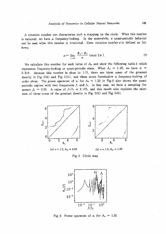
A rotation number can characterize such a mapping on the circle. When this number

is rational, we have a frequency-locking. In the meanwhile, a quasi-periodic behavior

can be seen when this number is irrational. Here, rotation nurnberpis defined as fol-

lows;

e.- e, (mod 2"). (7) p= lim n.co n

We calculate this number for each value of A. and show the following table.1 which

represents frequency-locking or quasi-periodic state. When A. = 1.20, we have p ==

O.319. Because this number is close to 1/3, there are three zones of -the greatest

density in Fig.2(b) and Fig.5(b), and these zones foreshadow a frequency-locking of

order three. The power spectrum of xi for A. == 1.20 in Fig.6 also shows the quasi-

periodic regime with two frequencies fi and fe. In this case, we have a sampling fre-

quency JEA = O.25. A value of filf2 is 3.125, and this result also explains the exist-

ence of three zones of the greatest density in Fig.3(b) and Fig.5(b).

-+me

6

4

2

o

/ti

･+--

c:st

en

(a) s=1.2,A. = O.69

Fig.5 Circle

6

4

2

.

lt.

.

:r'

:l'

2 4 6 en

(b) s= 1.2, A. = 1.20

map

lo2

looc.

e"" 10-2

10-4

fi

kh

m:

1O-2

Fig.6 Power spectrum

10'i 100flf,

of xi for A. == 1.20.

150 Toshihide TsuBATA, Hiroaki KAwABATA and Yoji TAKEDA

3-2. Intermittency

After the phase-locking state, quasi-periodic attractor becomes chaos via intermit-

tency. There are three types of intermittency, which are called type-I, type-ll and

type-M. Type-I intermittency is associated with the saddle-node bifurcation of the

limit cycle, type-I with a subcritical Hopf bifurcation, and type-M with a subcritical

period-doubling bifurcation')･8)･g)･ie?.

Fig.7(a)'y(c) show an output x2, and a route to chaos in this case is an intermitt-

ent one. A three-periodic oscillation changes into chaos via this intermittency. In

order to classify this intermittency, we show three fold circle maps in Fig.8. From

these figures, a saddle-node bifurcation is observed and we recognize that this intermi-

ttency can be classified as type-I.

1

pt

"o

-1

asenll , l,,,

lll Mki$sigfi ' it

li500 1000 1500

lteratlon

(a) A. = 3.82

1

o

g -1

-2

1

o,He:

-1

-- 2

.-"-s

sw n-e

500 10001500 lteratlon

(b) Am = 3･823

lo2

1oo

lo-2

lo-4

lo-G

'v'i h

ii,t ,u

.fli

al"I

Wereturn

consider

. map ls

fi

soo looolsoo lo-2 1o-i loe iteration tltA (c) Am =3･83 (d)

Fig.7 Time series of output x2

the return map which produces a type-I intermittency.

described as follows[7];

In+i = fr(In) = r+ In + alZ

In general, this

(8)

Analysis of Dynarnics in Cellular Neural Nbtworles 151

where a is constant andris a pararneter. When ris negative, map(6) has two fixed

points. These stability is controlled by fl(L)=1+2aL and one of them is stable,

which corresponds to the stable periodic oscillation before the onset of intermittency,

and the other point is unstable. When r = O, the two fixed points merge into semi-

stable fixed point. When r is positive, fixed points disappear and there is a narrow

channel between the diagonal and the graph of A(h), and this case corresponds to･the

saddlenode bifurcation shown in Fig.8. The trajectory travels slowly through the

channel from positive value of e(n) to negative value of e(n) in Fig.8. This nar-

row channel produces the laminar behavior of the intermittent state, and the regular

pulsing period is called "laminar length".

Table 1 Dynamical state with the rotation number and the largest

Lyapunov exponent for each value of A.

Am rotationnumber lar est L apunov ex onent d namicalstate

O.25 O.238 o.oo quasi-periodic

O.45 O.250(=4/16) -O.02 4:16 frequency-locking

O.69 O.254 o.oo quasi-periodic

O.85 O.273(==11/40) -O.04 11:40 frequency-locking

1.00 O.284(==7/25) -O.03 7:25 frequency-locking

1.20 O.319 o.oo quasi-periodic

2.00 O.333(=3/9) -O.18 3:9 frequency-locking

3.1 t"" 3.1 !. 3.1 ".3 "+.3 /// 'n.3 ./'"'igi[z .,// "t'ilg // .S :lg ,,,,i･'!

2.s 2.g 3 3.1 3.2 2･8 2･9 3 3･1 3･2 2.s 2.g 3 3.i 3.2

e. en e. (a) (b) (c) Fig.8 Three fold circle map

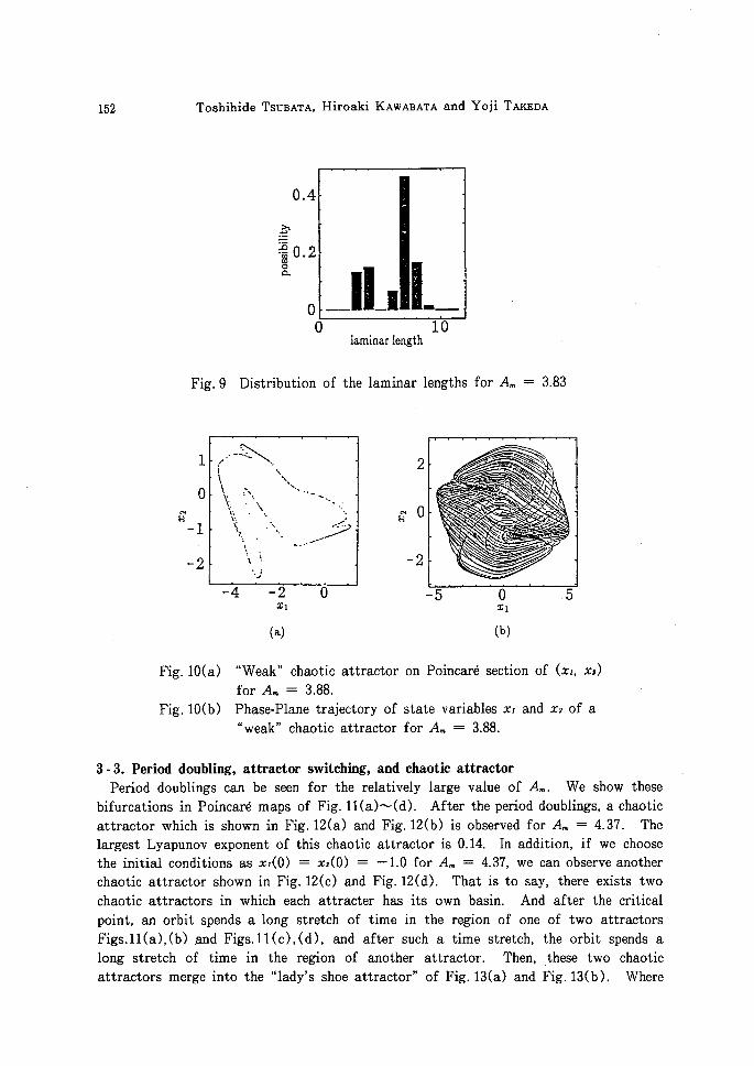
To clarify this type of intermittency further, we show a distribution of the laminar

length for A. = 3.83 in Fig. 9. The distribution of type- Ishows a maximum for long

laminar length, but that of type-I or type-M is exponentially falling towards long

length[7]. From this distribution nature of the larninar lengths, we also conclude that

intermittency in this case is typeI.

After this intermittent state, a "weak" chaotic attractor can be observed for A. =

3.88. For A. = 3.88, Fig. 10(a) shows a Poincare map, Fig. 10(b) a phase-plane tra-

jectory of state variables xi and sc2. The largest Lyapunov exponent in this case is

O.04. This attractor corresponds to a frame of the "lady's shoe attractor" [3], which

we will show in the next section.

152 Toshihide TSuBATA, Hiroaki KAwABATA and Yoji TAKEDA

h'tP.

8oa

O.4

O.2

o

--11N

g-.--

olarninar length

10

Fig.9 Distribution of the laminar lengths for A. = 3.83

1

o8 -1

-2

t " ' -fl:>xx

kN ,sv. :, s'N Vi '' ti, 1

-:- . x 1: , N･ -- 'Jt

N

N

.

.NsN

'

N s..l

-;-)?

."

･- 4 -2 Xl

(a)

o

2

N"O

-2

-5 oXl

(b)

,5

Fig. 10(a)

Fig. 10(b)

"Weak" chaotic attractor

for A. = 3.88.

Phase-Plane trajectory of

"weak" chaotic attractor

on Poincare sectlon

state variables xi

for A. = 3.88.

of (xi, xe)

and x2 of a

3-3. Period doubling, attractor switching, and chaotic attractor

Period doublings can be seen for the relatively 1arge value of A.. We show these

bifurcations in Poincar6 maps of Fig. 11(a)'y(d). After the period doublings, a chaotic

attractor which is shown in Fig. 12(a) and Fig. 12(b) is observed for A. == 4.37. The

largest Lyapunov exponent of this chaotic attractor is O.14. In addition, if we choose

the initial conditions as xi(O) = xe(O) = -1.0 for A. == 4.37, we can observe another

chaotic attractor shown in Fig. 12(c) and Fig. 12(d). That is to say, there exists two

chaotic attractors in which each attracter has its own basin. And after the critical

point, an orbit spends a long stretch of time in the region of one of two attractors

Figs.11(a),(b) .and Figs.11(c),(d), and after such a time stretch, the orbit spends a

long stretch of time in the region of another attractor. Then, .these two chaotic

attractors merge into the "lady's shoe attractor" of Fig. 13(a) and Fig. 13(b). Where

Analysis of Dynarnics in Cellular Nleural Nletworles 153

the largest Lyapunov exponent of this chaotic attractor is O.16. In a time-series plot

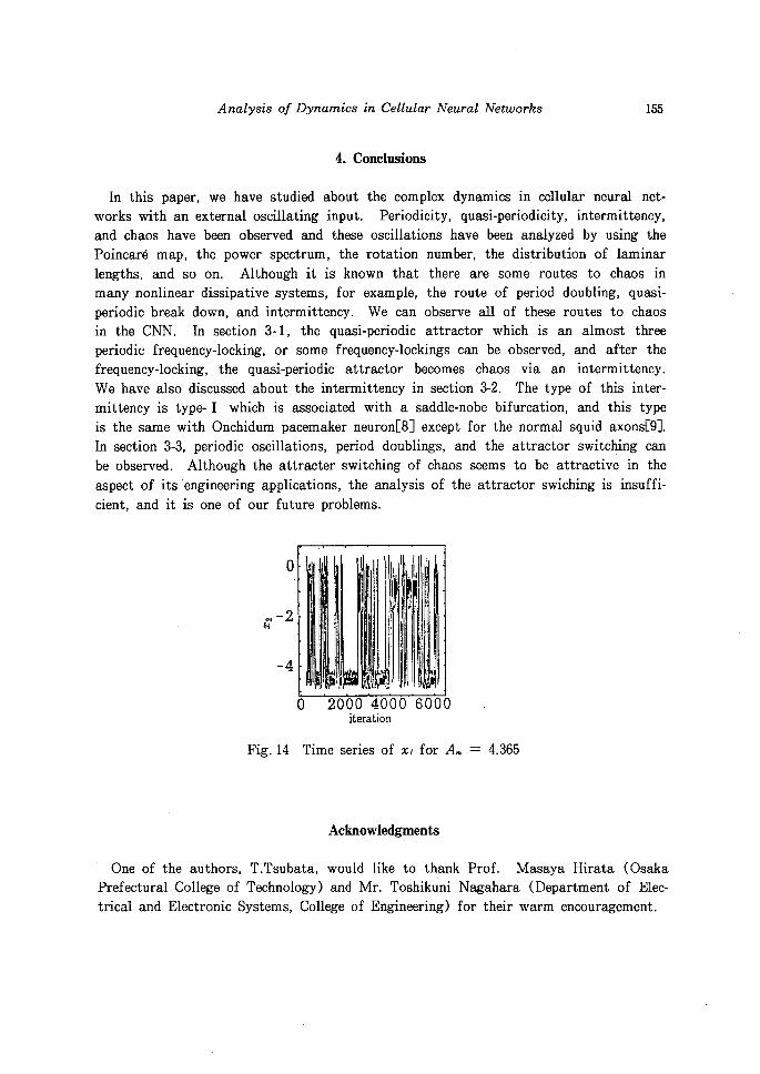
of the output x2, this switching (merging) is observed in Fig. 14 for A. = 4.365 when

the initial conditions are xi(O) = O.25 and xs(O) = O.15. In that way, the "lady's

shoe attractor" is produced via attractor switching (attractor merging)[11]. If we

take a value of A. smaller, this "lady's shoe attractor" becomes the weak chaotic

attractor of Figs. 10(a),(b). The larger a value of A. becornes, The larger fractal di-

mension of "lady's shoe attractor" becomes. It is one of our future problems to

analyse these process in detail.

8

1.5

1

O.5

.

-6 ･-4 Xl(a) A. = 5.0

g

1

O.9

8

.

-4.9-4.8-4.7-4.6 Xl (b) Am = 4･6

1

O.9

O.8

.

' .

-4'8 -4'6., -4'4

(c) A. =4.40

Fig. 11

1

O.9g

O.8

-t

..

.

. .'

-4.8

Poincar6 map

-4.6 -4.4 . Xl

(d) Am = 4･38

-- 4.I

IM Toshihide TsuBATA, Hiroaki KAwABATA and Yoji TAKEDA

1 /-K-. /2

O.9g ' I'. z;::,,:g:2,g, g O

O･8 1.V -2 -4.8 -4.6 -4.4 -4.2 -5 O XI XI (a) Am=4.37 (b) Am=4.37

'O･2 X. .,{,)=.1.o, 2Iglg Rx.<12{o)--i･o k,

""

- o.8

-1.5 -1 -O.5 -5 O Xi Xl (c) Am =: 4･37 (d) Am=4･37

Fig. 12 Bifurcations in Poincare section

(a) Chaotic attractor on Poincare section

(b) Phase-plane trajectory of state variables xi and

(c) Chaotic attractor on Poincare section

(d) Phaseplane trajectory of state variables xi and

5

･ N...ctf'llix;:I'"..':;;,

! d,." s. . :,..N:..

.X･.:: i.. ･ :i:.. t'p .. .. :･ .t. r.'.･ U" . '- 'N. i･{-,h,}i. 'x,-,<.,'･･,:ll'ltil:til･11.liif>

"s.` i;.. .."...:/.

.. N's' .- ::; :' - .

2

H" O

-2

5

X2

X2

1

.oe

-1

-4 -2 O -5 Xl

(a)

Fig. 13 The "lady's shoe attractor"

(a) Poincar6 section

(b) Phase-Plane trajectory

o Xl

(b)

for A. = 4.20

5

Analysis of Dynarrtics in Cellular Neural Nletworfes 155

4. Conclusions

In this paper, we have studied al)out the complex dynarnics in cellular neural net-

works with an external oscillating input. Periodicity, quasi-periodicity, intermittency,

and chaos have been observed and these oscillations have been analyzed by using the

Poincar6 map, the power spectrum, the rotation number, the distribution of laminar

lengths, and so on. Although it is known that there are some routes to chaos in

many nonlinear dissipative systems, for example, the route of period doubling, quasi-

periodic break down, and intermittency. We can observe al1 of these routes to chaos

in the CNN. In section 3-1, the quasi-periodic.attractor which is an almost three

periodic frequency-locking, or some frequency-lockings can be observed, and after the

frequency-locking, the quasi-periodic attractor becomes chaos via an intermittency.

We have also discussed about the intermittency in section 3-2. The type of this inter-

mittency is typeI which is associated with a saddle-nobe bifurcation, and this type

is the same with Onchidum pacemaker neuron[8] except for the normal squid axons[9].

In section 3-3, periodic oscillations, period doublings, and the attractor switching can

be observed. Although the attracter switching of chaos seems to be attractive in the

aspect of its engineering applications, the analysis of the attractor swiching is insuffi-

cient, and it is one of our future problems.

o

.- 2e

-4

Fig. 14

O 2000 4000 6000 lteratlon

Time series of xi for A. = 4.365

Acknowledgments

One of the authors, T.Tsubata, would like to thank Prof. Masaya Hirata (Osaka

Prefectural College of Technology) and Mr. Toshikuni Nagahara (Department of Elec-

trical and Electronic Systems, College of Engineering) for their warm encouragement.

1ss

[1]

[2]

[3]

[4]

[5]

[6]

[7]

[8]

[9]

[10]

[11]

Toshihide TsuBATA, Hiroaki KAwABATA and Yoji TAKEDA

References

'L.O.Chua and L.Yang: "Cellular Neural Networks: Theory", IEEE Trans. Cir-

cuits Syst., Vol. 35, No. 10 (1988)

L. O. Chua and L. Yang: "Cellular Neural Networks: Applications", IEEE Trans.

Circuits Syst., Vol. 35, No. 10 (1988)

F. Zou and J.A.Nossek: "A Chaotic Attractor with Cellular Neural Networks",

IEEE Trans. Circuits Syst., Vol.38, No.7 (1991)

L. O. Chua and T. Roska: "Stability of a Class of Nonreciprocal Cellular Neural

Networks", IEEE Trans. Circuits Syst., Vol. 37, No. 12 (1990)

T. Matsumoto, L. O. Chua, and H. Suzuki: "CNN cloning template: Shadow Detec-

tor", IEEE Trans. Circuits Syst., Vol. 37, No.8 (1990)

C.W.Wu, L.O.Chua, and T.Roska: "Two-Layer Radon Transform CellularNeural Network" IEEE Trans. Circuits Syst., Vol.39, No.7 (1992)

P.Berge, Y.Pomeau, and C.Vidal: "Order within Chaosa", Wiley, New York(1984)

H.Hayashi, S.Ishizuka, and K.Hirakawa: "Chaotic Responce of the Pacemaker

Neuron", J. Phys. Soc. Jpn., 54 (1985)

G.Matsurnoto, K.Aihara, et al.: "Chaos and phase locking in normal squid

axons" , Phys. Lett. A, 123 (1987)

T.Tsubata, H.Kawabata, et al.: "Intermittency of Recurrent Neuron and its

Network Dynarnics", IEICE Trans. Fundamentals, Vol. E76-A, No. 5 (1993)

C. Grebogi, E.Otto, F.Romeias, and J.A.Yorke: "Critical exponents for crisis-

induced intermittency", Phys. Rev. A, Vol.36, No. 11 (1987)