421 © IWA Publishing 2018 Hydrology Research | 49.2 | 2018

Timing of human-induced climate change emergence from

internal climate variability for hydrological impact studies

Mei-Jia Zhuan, Jie Chen, Ming-Xi Shen, Chong-Yu Xu, Hua Chen and

Li-Hua Xiong

ABSTRACT

This study proposes a method to estimate the timing of human-induced climate change (HICC)

emergence from internal climate variability (ICV) for hydrological impact studies based on climate

model ensembles. Specifically, ICV is defined as the inter-member difference in a multi-member

ensemble of a climate model in which human-induced climate trends have been removed through a

detrending method. HICC is defined as the mean of multiple climate models. The intersection

between HICC and ICV curves is defined as the time of emergence (ToE) of HICC from ICV. A case

study of the Hanjiang River watershed in China shows that the temperature change has already

emerged from ICV during the last century. However, the precipitation change will be masked by ICV

up to the middle of this century. With the joint contributions of temperature and precipitation, the

ToE of streamflow occurs about one decade later than that of precipitation. This implies that

consideration for water resource vulnerability to climate should be more concerned with adaptation

to ICV in the near-term climate (present through mid-century), and with HICC in the long-term future,

thus allowing for more robust adaptation strategies to water transfer projects in China.

doi: 10.2166/nh.2018.059

Mei-Jia ZhuanJie Chen (corresponding author)Ming-Xi ShenChong-Yu XuHua ChenLi-Hua XiongState Key Laboratory of Water Resources andHydropower Engineering Science,

Wuhan University,Wuhan 430072,ChinaE-mail: jiechen@whu.edu.cn

Chong-Yu XuDepartment of Geosciences,University of Oslo,P.O. Box 1047 Blindern, Oslo N-0316,Norway

Key words | climate change impacts, human-induced climate change, hydrology, internal climate

variability, time of emergence

INTRODUCTION

The Intergovernmental Panel on Climate Change (Pachauri

et al. ) states that consecutive changes of precipitation

pattern and temperature will give rise to a wide scope of

environmental and socio-economic impacts by the end of

the 21st century. Global climate change is driven on all time-

scales beyond that of individual weather events by internal

and external forcing (Pachauri et al. ). Internal forcing

includes naturally occurring processes in ocean and atmos-

phere, and interactions of ocean and atmosphere within

the climate system. Internal forcing exists as far back as

pre-industrial time, when the climate system was more

likely in an idealized state of climatic equilibrium with a

fixed atmospheric composition and an unchanging sun

(Pachauri et al. ). It gives rise to internal climate varia-

bility (ICV) which contributes to variations in climate. In

this way, ICV is natural fluctuations superimposed on a

stable average climate state in pre-industrial time or a

human-induced climate change (HICC) trend in industrial

time. Variations in climate may also result from external for-

cing of the climate system. External forcing consists of

anthropogenic forcing, such as greenhouse gas (GHG) emis-

sions and disruptive land use, and natural external forcing,

such as volcanic eruptions and solar variations. The

impact of volcanic eruptions generally lasts for less than a

decade (Pachauri et al. ), while solar variations take

place at multi-decadal, multi-centennial, and millennial

422 M.-J. Zhuan et al. | The role of internal climate variability in climate change hydrological impacts Hydrology Research | 49.2 | 2018

scales (Helama et al. ), which are considerably longer

than decades. However, the classical period for estimating

climate change is 30 years, as defined by the World Meteor-

ological Organization (Pachauri et al. ). Regardless of

climate change due to natural forcing with quite different

timescales (a few years for volcanic eruptions and tens of

thousands of years for solar radiation (Milankovitch

cycles)), climate change mainly consists of HICC and ICV.

The impact of climate change has received considerable

attention in recent literature, among which, the importance

of ICV has been discussed in several studies. For example,

Deser et al. (b) suggested presenting the role of ICV in

overall climate change on timescales of a few decades.

Fyfe et al. () claimed that ICV could help explain the

fact that recent observed global warming is significantly

less than that simulated by climate models. Swart et al.

() found that ICV can obscure or strengthen anthropo-

genic sea-ice loss at annual, decadal, and multi-decadal

timescales and should be properly considered in order to

interpret projections and evaluate models. Fyfe et al. ()

support the view that the effects of ICV imposed on HICC

have contributed to the global surface warming slowdown

or hiatus. In addition, Dai et al. () concluded that ICV,

mainly manifested in Interdecadal Pacific Oscillation, was

largely responsible for recent global warming slowdown,

as well as for earlier slowdowns and accelerations in

global-mean temperature, with preferred spatial patterns

different from those associated with human-induced warm-

ing or aerosol-induced cooling.

One of the other aspects of studying ICV is to investigate

its contribution to the uncertainty of climate change projec-

tions. For example, Hawkins & Sutton () quantified the

relative contribution of ICV to the uncertainty of global

temperature projections over the 21st century, using the

Coupled Model Intercomparison Project Phase 3 (CMIP3)

archive. They found that ICV contributed significantly to

the uncertainty of inter-decadal temperature before 2010.

A follow-up study by Hawkins & Sutton () for precipi-

tation at a regional scale showed that ICV was the

dominant source of uncertainty for decadal changes of pre-

cipitation in the first few decades of the 21st century. Deser

et al. (a) investigated the uncertainty in climate change

projections (surface air temperature, precipitation and sea

level pressure) arising from ICV, using a 40-member

ensemble of the National Center for Atmospheric Research

Community Climate System Model Version 3 (CCSM3)

under the A1B GHG emission scenario. Their results

showed that ICV accounts for at least half of the inter-

model uncertainty in projected climate (surface air tempera-

ture, precipitation, and sea level pressure) trends during

2005–2060. Deser et al. () also examined the contri-

bution of ICV to the uncertainty in projected surface air

temperature and precipitation trends during 2010–2060 at

local and regional scales over North America from large

ensembles of simulations with two comprehensive climate

models, the CCSM3 and the European Centre Hamburg

Model 5 (ECHAM5)-Max Planck Institute Ocean Model

(MPI-OM). This study showed that ICV has significant

impact on precipitation trends, and that intrinsic atmos-

pheric circulation variability is mainly responsible for the

uncertainty in future climate trends.

In addition to investigating the role and contribution of

ICV in climate projection, a few studies have quantified the

magnitude of ICV relative to HICC in overall climate

change using ‘time of emergence’ (ToE) as a criterion. ToE

is defined as the timing of when the magnitude of HICC

becomes greater than the noise of ICV (Hawkins & Sutton

). For example, Giorgi & Bi () defined HICC as

the mean precipitation change over models with multiple

projections, and ToE as the time when HICC emerges

from a combination of inter-model variability and ICV for

precipitation. Inter-model variability is defined as a variance

of individual model change time series after averaging over

the projections within each model. Regarding ICV itself,

different changes between each simulation and the ensem-

ble mean were obtained. Mahlstein et al. () estimated

HICC using the multi-model mean of summer average sur-

face temperature. Model data were first linearly detrended,

and then summer average surface temperatures were deter-

mined for each year. ICV was defined as ±2 standard

deviations of summer average surface temperature after

detrending. Hawkins & Sutton () assumed that HICC

of global mean surface air temperature follows a nonlinear

trend. Thus, a fourth-order polynomial was used to fit the

annual temperature. ICV was defined as the inter-annual

standard deviation of seasonal (or annual) mean tempera-

tures, using pre-industrial control simulations assumed

without anthropogenic forcing. Their study implies that

423 M.-J. Zhuan et al. | The role of internal climate variability in climate change hydrological impacts Hydrology Research | 49.2 | 2018

ToE is a basic property of climate system, the true values of

which are unknown, but which can be estimated using

model simulations. Similarly, Maraun () defined HICC

as the multi-model mean of precipitation. Model data were

first linearly detrended by a parametric trend model, and

then ICV was defined as the inter-annual variability

measured by the standard deviation of the detrended

model data.

Even though the magnitude of ICV relative to HICC has

been investigated in some studies, far fewer studies have dis-

cerned the timing of HICC’s departure from ICV for

hydrological climate change impact studies. For example,

Leng et al. () detected the emergence of hydrologic

changes in surface water resources in the conterminous

United States under future warming. They used a two-

sample Kolmogorov–Smirnov test to compare the prob-

ability distribution functions of historical and future

streamflows. The emergence of significant changes is

defined as the time when the future distribution differs sig-

nificantly from the reference period, and when the

distributions in all subsequent 30-year periods also differ sig-

nificantly from the reference period. This study did not

separately estimate HICC and ICV to find ToE.

Moreover, since ICV manifests itself at various temporal

and spatial scales, there are many modes of ICV for climate

system. Hawkins & Sutton () and Maraun () investi-

gated inter-annual variability and defined the ToE of climate

Figure 1 | Location of the Hanjiang River watershed.

change signal as a specific year; while others (e.g., Giorgi &

Bi ; Mahlstein et al. ; Leng et al. ) investigated

multi-decadal variability and defined the ToE as a period

of 20 or 30 years. Since climate change impact studies are

commonly conducted for multi-year periods (e.g., of 30

years) (Pachauri et al. ), it may be more reasonable to

estimate ICV at a multi-decadal timescale when the goal is

to investigate the role of ICV in climate change impact

studies. In addition, ToE estimated for a multi-year period

may be more reliable and credible, since inter-annual varia-

bility is mostly smoothed by calculating the multi-year

average.

The main objective of this study is to propose a method

to estimate the timing of climate change emergence from

ICV for hydrological impact studies based on a multi-

member ensemble of a climate model. Hanjiang River water-

shed above the Danjiangkou reservoir (in China) is selected

to exemplify the proposed method.

STUDY AREA AND DATA

Study area

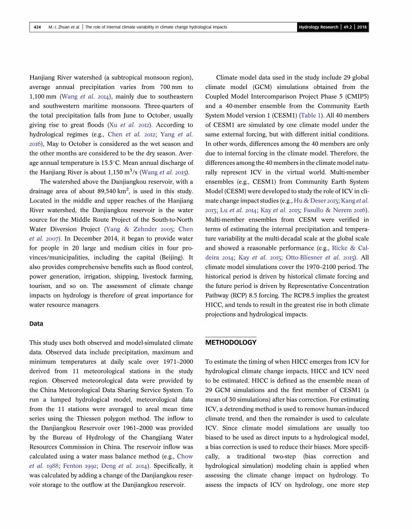
The Hanjiang River has a mainstream river length of 1,577

km and a drainage area of 159,000 km2 (Figure 1). It is one

of the longest tributary rivers of the Yangtze River. In the

424 M.-J. Zhuan et al. | The role of internal climate variability in climate change hydrological impacts Hydrology Research | 49.2 | 2018

Hanjiang River watershed (a subtropical monsoon region),

average annual precipitation varies from 700 mm to

1,100 mm (Wang et al. ), mainly due to southeastern

and southwestern maritime monsoons. Three-quarters of

the total precipitation falls from June to October, usually

giving rise to great floods (Xu et al. ). According to

hydrological regimes (e.g., Chen et al. ; Yang et al.

), May to October is considered as the wet season and

the other months are considered to be the dry season. Aver-

age annual temperature is 15.5�C. Mean annual discharge of

the Hanjiang River is about 1,150 m3/s (Wang et al. ).

The watershed above the Danjiangkou reservoir, with a

drainage area of about 89,540 km2, is used in this study.

Located in the middle and upper reaches of the Hanjiang

River watershed, the Danjiangkou reservoir is the water

source for the Middle Route Project of the South-to-North

Water Diversion Project (Yang & Zehnder ; Chen

et al. ). In December 2014, it began to provide water

for people in 20 large and medium cities in four pro-

vinces/municipalities, including the capital (Beijing). It

also provides comprehensive benefits such as flood control,

power generation, irrigation, shipping, livestock farming,

tourism, and so on. The assessment of climate change

impacts on hydrology is therefore of great importance for

water resource managers.

Data

This study uses both observed and model-simulated climate

data. Observed data include precipitation, maximum and

minimum temperatures at daily scale over 1971–2000

derived from 11 meteorological stations in the study

region. Observed meteorological data were provided by

the China Meteorological Data Sharing Service System. To

run a lumped hydrological model, meteorological data

from the 11 stations were averaged to areal mean time

series using the Thiessen polygon method. The inflow to

the Danjiangkou Reservoir over 1961–2000 was provided

by the Bureau of Hydrology of the Changjiang Water

Resources Commission in China. The reservoir inflow was

calculated using a water mass balance method (e.g., Chow

et al. ; Fenton ; Deng et al. ). Specifically, it

was calculated by adding a change of the Danjiangkou reser-

voir storage to the outflow at the Danjiangkou reservoir.

Climate model data used in the study include 29 global

climate model (GCM) simulations obtained from the

Coupled Model Intercomparison Project Phase 5 (CMIP5)

and a 40-member ensemble from the Community Earth

SystemModel version 1 (CESM1) (Table 1). All 40 members

of CESM1 are simulated by one climate model under the

same external forcing, but with different initial conditions.

In other words, differences among the 40 members are only

due to internal forcing in the climate model. Therefore, the

differences among the 40members in the climatemodel natu-

rally represent ICV in the virtual world. Multi-member

ensembles (e.g., CESM1) from Community Earth System

Model (CESM)were developed to study the role of ICV in cli-

mate change impact studies (e.g.,Hu&Deser ; Kang et al.

; Lu et al. ; Kay et al. ; Fasullo & Nerem ).

Multi-member ensembles from CESM were verified in

terms of estimating the internal precipitation and tempera-

ture variability at the multi-decadal scale at the global scale

and showed a reasonable performance (e.g., Ricke & Cal-

deira ; Kay et al. ; Otto-Bliesner et al. ). All

climate model simulations cover the 1970–2100 period. The

historical period is driven by historical climate forcing and

the future period is driven by Representative Concentration

Pathway (RCP) 8.5 forcing. The RCP8.5 implies the greatest

HICC, and tends to result in the greatest rise in both climate

projections and hydrological impacts.

METHODOLOGY

To estimate the timing of when HICC emerges from ICV for

hydrological climate change impacts, HICC and ICV need

to be estimated. HICC is defined as the ensemble mean of

29 GCM simulations and the first member of CESM1 (a

mean of 30 simulations) after bias correction. For estimating

ICV, a detrending method is used to remove human-induced

climate trend, and then the remainder is used to calculate

ICV. Since climate model simulations are usually too

biased to be used as direct inputs to a hydrological model,

a bias correction is used to reduce their biases. More specifi-

cally, a traditional two-step (bias correction and

hydrological simulation) modeling chain is applied when

assessing the climate change impact on hydrology. To

assess the impacts of ICV on hydrology, one more step

Table 1 | General information of 30 GCMs used

Modeling center Institution Model name

Horizontalresolution(lon. × lat.) ID

CSIRO-BOM CSIRO (Commonwealth Scientific and Industrial Research OrganisationAustralia), and BOM (Bureau of Meteorology, Australia)

ACCESS1.0 1.875 × 1.25 1ACCESS1.3 1.875 × 1.25 2

BCC Beijing Climate Center, China Meteorological Administration BCC-CSM1.1 2.8 × 2.8 3BCC-CSM1.1(m) 1.125 × 1.125 4

GCESS College of Global Change and Earth System Science, Beijing NormalUniversity

BNU-ESM 2.8 × 2.8 5

CCCma Canadian Centre for Climate Modelling and Analysis CanESM2 2.8 × 2.8 6CESM1-CAM5 1.25 × 0.9 7

NCAR National Center for Atmospheric Research CESM1 1.25 × 0.9 8

CMCC Centro Euro-Mediterraneo per I Cambiamenti Climatici CMCC-CESM 3.75 × 3.7 9CMCC-CM 0.75 × 0.7 10CMCC-CMS 1.875 × 1.875 11

CNRM-CERFACS Centre National de Recherches Météorologique/Centre Européen deRecherche et de Formation Avancée en Calcul Scientifique

CNRM-CM5 1.4 × 1.4 12

CSIRO-QCCCE Commonwealth Scientific and Industrial Research Organisation incollaboration with the Queensland Climate Change Centre of Excellence

CSIRO-Mk3.6.0 1.875 × 1.875 13

ICHEC Irish Centre for High-End Computing EC-EARTH 1.1 × 1.1 14

LASG-CESS LASG, Institute of Atmospheric Physics, Chinese Academy of Sciences; andCESS, Tsinghua University

FGOALS-g2 1.875 × 1.25 15

NOAA-GFDL Geophysical Fluid Dynamics Laboratory GFDL-CM3 2.5 × 2.0 16GFDL-ESM2G 2.5 × 2.0 17GFDL-ESM2M 2.5 × 2.0 18

NIMR-KMA National Institute of Meteorological Research HadGEM2-AO 1.875 × 1.25 19

MOHC Met Office Hadley Centre HadGEM2-CC 1.875 × 1.25 20HadGEM2-ES 1.875 × 1.25 21

INM Institute for Numerical Mathematics INM-CM4 2.0 × 1.5 22

IPSL Institut Pierre-Simon Laplace IPSL-CM5A-LR 3.75 × 1.875 23IPSL-CM5A-MR 2.5 × 1.25 24IPSL-CM5B-LR 3.75 × 1.875 25

MPI-M Max Planck Institute for Meteorology MPI-ESM-LR 1.875 × 1.8 26MPI-ESM-MR 1.875 × 1.8 27

MRI Meteorological Research Institute MRI-CGCM3 1.125 × 1.125 28MRI-ESM1 1.1 × 1.1 29

NCC Norwegian Climate Centre NorESM1-M 2.5 × 1.9 30

425 M.-J. Zhuan et al. | The role of internal climate variability in climate change hydrological impacts Hydrology Research | 49.2 | 2018

(detrending) is added in the modeling chain to remove cli-

mate trend from the CESM1 ensemble. The other two

steps are the same. More details are given below.

Detrending methods

A two-stage detrending method was used to remove climate

trend from the CESM1 ensemble. The climate trend is

assumed to follow a linear trend. Since all CESM1 members

are simulated using the same model structure and driven by

identical climate forcing, it is expected that all members

include the same climate trend. Thus, the climate trend is

estimated based on a 40-member ensemble mean.

Since the CESM1 simulations are driven by different for-

cings during the historical period (1970–2005) and the

future period (2006–2100), the climate trend may be

426 M.-J. Zhuan et al. | The role of internal climate variability in climate change hydrological impacts Hydrology Research | 49.2 | 2018

different between these two periods. Thus, a two-stage

method is used to detect and remove trends of climate

change for the two periods separately. For each period, a

Mann–Kendall test is used to discern if a significant trend

exists. In the first stage, if a significant trend exists in the his-

torical period, the Mann–Kendall test is further used to find

a breakpoint that separates the historical period into sub-

periods with and without a climate trend. In other words,

the first sub-period is free of human-induced climate trend,

while the detected trend begins at the breakpoint and

extends throughout the second sub-period. Since several

breakpoints may exist when using the Mann–Kendall test,

the sum of squared errors (SSE) is used as a criterion to

find the real breakpoint, which can best distinguish the

two sub-periods. The SSE of prediction is calculated based

on the mean value over the first sub-period and the fitted

linear trend over the second sub-period. To detrend the cli-

mate trend for the historical period, the first sub-period is

assumed to be unchanged, while a linear curve is fitted to

the second sub-period with its first point forced to pass

through the mean of the first sub-period; that same trend

is then removed from each of the 40 members. In the

second stage if a significant trend exists for the future

period, a linear curve is fitted to the ensemble mean of the

40 members. The same trend is then removed from each

of the 40 members. The difference between the mean

values of the historical and future periods is removed in

the last step. The observed precipitation and mean tempera-

ture may also contain climate trends. If the Mann–Kendall

test shows a significant trend, the first stage of the above

method is used to remove the climate trend for the single

time series. ICV is the residual of the data after the trend

removal step.

Bias correction

A quantile mapping bias correction was used to correct the

bias for a multi-member ensemble of CESM1 and 29 climate

model simulations. This method (Schmidli et al. ;

Mpelasoka & Chiew ; Chen et al. ) is a combination

of the Daily Transition (DT) (Mpelasoka & Chiew ) and

Local Intensity Scaling (LOCI) (Schmidli et al. ; Chen

et al. b) methods, and is known as daily bias correction

(DBC) in Chen et al. (). The LOCI method is first used to

correct precipitation occurrence, insuring that the frequency

of precipitation occurrence of corrected data at the refer-

ence period is equal to that of observed data for each

month. Next, the DT method is applied to correct the fre-

quency distribution of precipitation amounts and

temperatures based on quantile differences between model

data and observed data.

The DBC method was calibrated at a historical period

(1971–2000) and applied to multiple 30-year periods. The

multiple periods are sliding 30-year time windows that

vary by one year, e.g., 1970–1999, 1971–2000, 1972–2001,

etc., over the whole period (1970–2100), totaling 102

periods. When correcting CESM1, all members were

pooled together to estimate bias correction factors. In

other words, correction factors were estimated as the differ-

ence between observed data and all the members of the

model data during a reference period (1971–2000). For

each of the 40 ensemble members, correction factors,

assumed to be constant over time, were applied to model

data for the whole period (1970–2100). All the members of

CESM1 are treated as a whole because all CESM1 members

were simulated using the same climate model with identical

climate forcing, and therefore it is expected that all members

have the same model biases. When correcting the other 29

GCM simulations, correction factors were estimated for

each GCM simulation. In other words, each climate simu-

lation was corrected individually.

Hydrological simulation

The hydrological modeling was carried out using a lumped

conceptual rainfall–runoff model, HMETS, developed at

the École de technologie supérieure, University of Quebec

(Martel et al. ). HMETS has been used in a number of

flow prediction and climate change impact studies (e.g.,

Arsenault et al. ; Chen et al. ). It accounts for evapo-

transpiration, infiltration, snow accumulation, melting and

refreezing processes, and flow routing to a watershed’s

outlet. The model has up to 21 free parameters: one for eva-

potranspiration, ten for snow accumulation and snowmelt,

four for vertical water balance, and six for horizontal

water movement. For rainfall-dominated watersheds (as is

the case in this study), HMETS’ snow module is not used,

and so the model used in this study has 11 parameters to

427 M.-J. Zhuan et al. | The role of internal climate variability in climate change hydrological impacts Hydrology Research | 49.2 | 2018

be determined. The required daily input data for HMETS are

the daily averaged precipitation and daily mean air tempera-

ture. If the maximum and minimum temperatures are input

to the model, they are automatically averaged to the mean

temperature. The daily inflow discharge time series is also

used for calibration (1961–1980) and validation (1981–

2000) purpose.

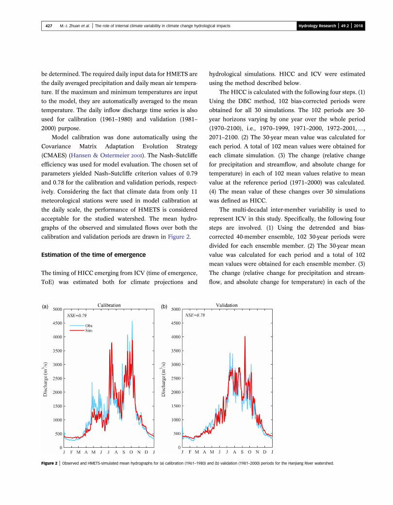
Model calibration was done automatically using the

Covariance Matrix Adaptation Evolution Strategy

(CMAES) (Hansen & Ostermeier ). The Nash–Sutcliffe

efficiency was used for model evaluation. The chosen set of

parameters yielded Nash–Sutcliffe criterion values of 0.79

and 0.78 for the calibration and validation periods, respect-

ively. Considering the fact that climate data from only 11

meteorological stations were used in model calibration at

the daily scale, the performance of HMETS is considered

acceptable for the studied watershed. The mean hydro-

graphs of the observed and simulated flows over both the

calibration and validation periods are drawn in Figure 2.

Estimation of the time of emergence

The timing of HICC emerging from ICV (time of emergence,

ToE) was estimated both for climate projections and

Figure 2 | Observed and HMETS-simulated mean hydrographs for (a) calibration (1961–1980) a

hydrological simulations. HICC and ICV were estimated

using the method described below.

The HICC is calculated with the following four steps. (1)

Using the DBC method, 102 bias-corrected periods were

obtained for all 30 simulations. The 102 periods are 30-

year horizons varying by one year over the whole period

(1970–2100), i.e., 1970–1999, 1971–2000, 1972–2001,…,

2071–2100. (2) The 30-year mean value was calculated for

each period. A total of 102 mean values were obtained for

each climate simulation. (3) The change (relative change

for precipitation and streamflow, and absolute change for

temperature) in each of 102 mean values relative to mean

value at the reference period (1971–2000) was calculated.

(4) The mean value of these changes over 30 simulations

was defined as HICC.

The multi-decadal inter-member variability is used to

represent ICV in this study. Specifically, the following four

steps are involved. (1) Using the detrended and bias-

corrected 40-member ensemble, 102 30-year periods were

divided for each ensemble member. (2) The 30-year mean

value was calculated for each period and a total of 102

mean values were obtained for each ensemble member. (3)

The change (relative change for precipitation and stream-

flow, and absolute change for temperature) in each of the

nd (b) validation (1981–2000) periods for the Hanjiang River watershed.

428 M.-J. Zhuan et al. | The role of internal climate variability in climate change hydrological impacts Hydrology Research | 49.2 | 2018

102 mean values relative to mean value at the reference

period (1971–2000) was calculated. (4) The standard devi-

ation of these changes over 40 members was calculated for

each period and a total of 102 standard deviation values

were obtained. ICV was then defined as ±2 standard devi-

ations of inter-member differences. According to the ‘3σ’

principle of normal distribution, the chance for absolute

values of climate change (attributed to ICV) to exceed þ2

standard deviations of inter-member differences is only

2.3% and the same is true for �2 standard deviations

(Hansen et al. ). Therefore, when absolute values of cli-

mate change become greater than ±2 standard deviations of

inter-member differences, the climate change is most likely

to be attributed to HICC. A similar method has also been

used in other studies (e.g., Hulme et al. ; Mahlstein

et al. ; Hansen et al. ; Stocker et al. ).

With the above steps, 102 HICC values form a curve and

102 ICV values form another curve; the intersection of these

two curves is defined as the ToE. If an HICC curve inter-

sects an ICV curve of þ2 standard deviations, it implies

that there is an increasing climate change trend. If an

HICC curve intersects an ICV curve of �2 standard devi-

ations, then there is a decreasing climate change trend. No

intersection implies that HICC does not emerge from ICV

or that there is no obvious HICC. To produce conservative

adaptation strategies for HICC impacts, ±1 standard devi-

ation is also calculated. The period between the

intersections of ±2 and ±1 standard deviations is defined

as an unpredictable time period. The same procedure was

carried out for precipitation, mean temperature, and stream-

flow at annual and seasonal scales (wet season: May to

October; dry season: January to April and November to

December). The dry and wet seasons were defined based

on climatic and hydrological regimes in the Hanjiang

River watershed.

RESULTS

Performance of the detrending method

The detrending method was applied to mean temperature

and precipitation time series over the 1971–2000 reference

period for observations and over the 1970–2100 period for

a CESM1 40-member ensemble. Figure 3 presents the

detrending results for mean temperature and precipitation

of a CESM1 40-member ensemble at annual and seasonal

timescales. For this specific watershed, annual and wet

season mean temperatures show little trend, while dry

season mean temperature shows a significant decreasing

trend for the historical period tested by the Mann–Kendall

test at the p¼ 0.05 significant level. However, annual and

seasonal mean temperatures exhibit a significant increasing

trend for the future period. For annual and seasonal precipi-

tation, a significant downtrend is observed for the historical

period, while a significant uptrend is observed for the future

period. The detrending method performs reasonably well in

terms of removing the trend of the multi-member ensemble.

Residual ensemble spread represents ICV, which obviously

has been preserved throughout the detrending process,

since fluctuations and ensemble spread remain almost the

same with raw data for the same time series.

Performance of the bias correction method

To verify the performance of bias correction in correcting

multi-member ensemble, the multi-member ensemble of

CESM1 mean temperature and precipitation is compared

to the observed counterparts for the reference period

(1971–2000). Figure 4 presents empirical cumulative distri-

bution functions (CDFs) of the detrended annual mean

temperature and precipitation for raw and bias-corrected

40-member ensembles of CESM1. The empirical cumulative

distribution function (e.g., F(x)) is defined as the ratio of the

number (e.g., a) of annual mean temperatures or annual pre-

cipitations that are less than a certain value (e.g., x) and

sample size (e.g., n) plus one (i.e., F(x)¼ a/(nþ 1)). For

each empirical probability, a horizontal range was con-

structed by 40 values corresponding to 40 members of

CESM1. All members were pooled together to plot an

empirical CDF curve and CDFs for observed annual mean

temperature and precipitation were also plotted for

comparison.

For raw model data, wet biases are observed for annual

precipitation and cool biases are observed for annual mean

temperature. In other words, the CESM1 ensemble underes-

timates annual mean temperature and overestimates

annual precipitation. After bias correction, wet biases in

Figure 3 | Raw and detrended CESM1 (a)–(c) mean temperature and (d)–(f) precipitation time series at annual and seasonal timescales, respectively, over the 1970–2100 period in the

Hanjiang River watershed. Shades show the ranges of precipitation or temperature ensembles with and without detrending, respectively. The wave curves show the ensemble

means for non-detrended and detrended data, respectively. Skew lines are the best-fit linear trends to the non-detrended wave curves for the second historical sub-period and

the future period, respectively.

Figure 4 | Empirical cumulative distribution functions (CDFs) for annual (a) mean temperature and (b) precipitation. RA: all raw 40 members; CA: all corrected 40 members; Obs: observed

data; RS: each of the raw 40 members and the asterisk symbols represent the spread of the 40 ensemble members; CS: each of the corrected 40 members and the asterisk

symbols represent the spread of the 40 ensemble members.

429 M.-J. Zhuan et al. | The role of internal climate variability in climate change hydrological impacts Hydrology Research | 49.2 | 2018

430 M.-J. Zhuan et al. | The role of internal climate variability in climate change hydrological impacts Hydrology Research | 49.2 | 2018

precipitation and cool biases in mean temperature were

removed, as indicated by the fact that the CDFs of corrected

ensembles are almost identical to those of observed data for

both mean temperature and precipitation. This result proves

the good performance of bias correction in terms of remov-

ing bias from multi-member ensemble means.

In a departure from traditional studies that use single cli-

mate simulation, this study used a bias correction method

for a multi-member ensemble. This approach should not

only reduce the biases of climate model outputs, but also

preserve the simulated ICV. ICV can be represented by a

spread of 40 CDFs corresponding to 40 CESM1 members.

If the bias correction was conducted for each member

individually, the CDFs of all members should be almost

identical to observed CDFs. Figure 4 shows that, after bias

correction, the spread of the 40 ensemble members remains

Figure 5 | Mean hydrographs simulated by (a) raw and (b) corrected climate data for reference p

percentile high flow and (d) annual 5th percentile low flow for the same period. Mod

annual flows; CA: all corrected 40 members of annual flows; OBs: observed data of an

of the 40 ensemble members; CS: each of the corrected 40 members and the aste

almost the same as those of raw model data for temperature

and precipitation. This indicates the reasonable perform-

ance of the bias correction methods in terms of preserving

the inter-member variability of multi-member ensembles.

Performance of hydrological simulation

Figure 5(a) and 5(b) show mean hydrographs simulated by

raw and corrected climate simulations, respectively. Specifi-

cally, hydrographs were calculated by averaging daily

streamflows over a 30-year reference period (1971–2000)

for each of 40 members. Figure 5(c) and 5(d) present empiri-

cal CDFs of annual 95th percentile high flow and annual 5th

percentile low flow. The empirical CDFs of high and low

flows were calculated as with those of precipitation and

temperature in Figure 4.

eriod (1971–2000) and empirical cumulative distribution functions (CDFs) of (c) annual 95th

: hydrographs of ensemble; Obs: hydrograph of observed data; RA: all raw 40 members of

nual flows; RS: each of the raw 40 members and the asterisk symbols represent the spread

risk symbols represent the spread of the 40 ensemble members.

431 M.-J. Zhuan et al. | The role of internal climate variability in climate change hydrological impacts Hydrology Research | 49.2 | 2018

The raw CESM1 ensemble considerably overestimates

mean, high and low flows. The 40-member ensemble

hydrograph envelope simulated by raw data is totally

beyond the hydrograph simulated by observed climate

data. Similar results are also observed for high and low

flows, as empirical CDFs are all greater than counterparts

of observed data. This was as expected, because the

CESM1 ensemble overestimates precipitation and underes-

timates temperature. With bias correction, the 40-member

hydrograph envelope covers the observed counterpart,

and also the envelope of empirical CDFs embraces the

observed counterpart for both high and low flows. This

indicates that the model bias in climate data has been

removed and so the hydrological simulation is reliable.

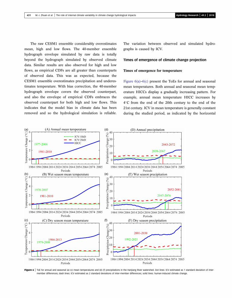
Figure 6 | ToE for annual and seasonal (a)–(c) mean temperatures and (d)–(f) precipitations in

member differences; dash lines: ICV estimated as 2 standard deviations of inter-m

The variation between observed and simulated hydro-

graphs is caused by ICV.

Times of emergence of climate change projection

Times of emergence for temperature

Figure 6(a)–6(c) present the ToEs for annual and seasonal

mean temperatures. Both annual and seasonal mean temp-

erature HICCs display a gradually increasing pattern. For

example, annual mean temperature HICC increases by

4�C from the end of the 20th century to the end of the

21st century. ICV in mean temperature is generally constant

during the studied period, as indicated by the horizontal

the Hanjiang River watershed. Dot lines: ICV estimated as 1 standard deviation of inter-

ember differences; solid lines: human-induced climate change.

432 M.-J. Zhuan et al. | The role of internal climate variability in climate change hydrological impacts Hydrology Research | 49.2 | 2018

curve. In addition, ICV is small for annual and seasonal

mean temperatures, as it is less than 0.5�C. Both annual

and seasonal mean temperature HICCs first increase

slowly and then faster, and then after a certain point they

increase steadily. For example, annual mean temperature

HICC increases slowly from the period 1971–2000 to the

period 1980–2009. It then increases at a rate that gradually

becomes greater until period 2017–2046; thereafter, the

rate of increase stays relatively constant.

Two curves intersect at the 1981–2010 period for annual

mean temperature, at the 1981–2010 period for wet season

mean temperature, and at the 1984–2013 period for dry

season mean temperature. When using ±1 standard devi-

ation to represent ICV, the ToE will move backwards by

around five years.

Times of emergence for precipitation

Figure 6(d)–6(f) presents the ToE for annual and seasonal

precipitations. In contrast to mean temperature changes,

annual and wet season precipitation HICCs first show a

slight decreasing trend until the 2030s, and then they start

gradually increasing. Dry season precipitation HICC

shows a significant increasing pattern over the 1970–2100

period. Wet season precipitation HICC contributes more

to annual precipitation HICC, as rainfall in the studied

watershed mainly happens in the wet season. ICV is gener-

ally constant during the 1970–2100 period.

The HICC curve crosses the ICV curve at the 2043–2072

period for annual precipitation, at the 2052–2081 period for

wet season precipitation, and at the 2001–2030 period for

dry season precipitation, respectively. When using ±1 stan-

dard deviation to represent ICV, the ToE will move

backwards by about ten years.

Times of emergence for hydrological impact

Figure 7(a)–7(c) present the ToE for annual and seasonal

mean streamflows. The results show that the human-

induced change in annual and wet season mean streamflows

display a slight decreasing trend until the 2030s and then

they start to increase gradually; while for the dry season

streamflow, the turning point is at the 2000s.

The HICC curve crosses the ICV curve at the 2055–2084

period for annual mean streamflow, at the 2056–2085 period

for wet season mean streamflow, and at the 2061–2090

period for dry season mean streamflow, respectively. This

indicates that the human-induced changes in annual and

seasonal streamflows are likely to move out of the range of

the internal streamflow variability in the second half of the

21st century. When using ±1 standard deviation to rep-

resent ICV, the ToE will move backwards by around ten

years, in particular for annual and wet season mean

streamflows.

DISCUSSION

This study investigated the importance of ICV relative to

HICC in hydrological climate change impact studies. To

achieve this, a method to estimate the ToE of climate projec-

tions and hydrological simulations is proposed. This method

estimates ICV based on the spread of a multi-member

ensemble, and HICC based on the mean over multi-model

projections together with that of a multi-member ensemble.

A case study was conducted on the Hanjiang River

watershed.

The results show that the ToE of mean temperature has

already occurred during the end of the last century and the

beginning of this century, but this is not the case for precipi-

tation. Instead, for precipitation, the ToE is projected to

occur around the 2050s, several decades later than for

mean temperature. ICV for precipitation is large enough to

obscure HICC for precipitation for the next few decades of

the 21st century, until the constantly increasing HICC

becomes greater thereafter. With the joint contribution of

temperature and precipitation, ToE of mean streamflow

occurs about one decade later than that of precipitation,

near the horizon of 2100. This is as expected, because the

increase in temperature partly offsets the increase in stream-

flow resulting from precipitation increase through the

increase in evapotranspiration.

The estimated ToE is dependent on how ICV and HICC

are defined. In other words, different methods in estimating

ICV and HICC may result in different ToE. This study

defined HICC as a multi-model ensemble mean. Even

though some individual climate model simulations may

Figure 7 | ToE for annual and seasonal mean streamflows in the Hanjiang River watershed. Dot lines: ICV estimated as 1 standard deviation of inter-member differences; dash lines: ICV

estimated as 2 standard deviations of inter-member differences; solid lines: human-induced climate change.

433 M.-J. Zhuan et al. | The role of internal climate variability in climate change hydrological impacts Hydrology Research | 49.2 | 2018

not be reliable in calculating the climate change signal, due

to model uncertainty and climate variability, the multi-

model ensemble mean can be considered as a more reliable

solution, since the climate variability and model uncertainty

are largely filtered out (Giorgi & Bi ; Mahlstein et al.

; Maraun ). When calculating the ensemble mean,

all climate projections were considered equiprobable in

this study. However, other studies (e.g., Giorgi & Mearns

, ; Hawkins & Sutton ) proposed that climate

models should be weighted based on their ability to better

represent various metrics over a reference period. Weighting

climate model simulation is controversial when using mul-

tiple climate models for impact studies; and is especially

so between climate modeling and impact assessment com-

munities. However, a recent study (Chen et al. )

showed that weighting GCMs has a limited impact on pro-

jected future climate both in terms of precipitation and

temperature changes and hydrological impacts.

The magnitude of HICC is also dependent on the GHG

emission scenario. Thus, the estimated ToE may also be sen-

sitive to the GHG emission scenario, as has been pointed

out in some studies (e.g., Giorgi & Bi ). The magnitude

of GHG-forced precipitation changes tends to become

greater as the GHG forcing increases (Giorgi & Bi ).

The alternative scenarios for anthropogenic emissions give

rise to changes in the ToE by a magnitude of a decade or

more (Hawkins & Sutton ). For example, warm scen-

arios tend to lead to earlier ToE, while lower levels of

emissions result not only in later ToE, but also in a more gra-

dual rise in temperature HICC, thus producing a large

increase in the uncertainty of ToE (Hawkins & Sutton

). In order to make a conservative decision to counter

climate change impacts, only one extreme GHG emission

scenario is used to estimate HICC in this study.

ICV has been defined as the inter-member difference of

a climate model. Since these ensemble members are

434 M.-J. Zhuan et al. | The role of internal climate variability in climate change hydrological impacts Hydrology Research | 49.2 | 2018

projected within the same model structure and under the

same forcing, inter-member difference can be considered

as ICV. In other words, different ensemble members show

how much climate can vary in the model world as a result

of random internal variations. To the extent that the

model simulates relevant physical processes, the range of

ensemble provides insight into what could happen in the

single realization that will occur in the real world (Deser

et al. a, b). The same method has been used in sev-

eral previous studies (e.g., Hulme et al. ; Deser et al.

a, b; Fatichi et al. ). The results showed that

multi-member ensemble of climate models can represent

the observed ICV well at both regional and global scale.

However, it should be noted that ICV is inherently complex

and manifests itself over various temporal and spatial scales.

This study only used multi-decadal variability to represent

ICV at the multi-decadal scale. Multi-decadal variability is

just one component of ICV, even though it is one of the

key components for most climate change impact studies.

Although some studies (e.g., Hawkins & Sutton ;

Maraun ) defined the ToE as a specific year, the ToE

estimated for a multi-year period may be more reliable and

credible, since inter-annual variability is mostly filtered out

by calculating multi-year averages. Moreover, climate

change impact studies are commonly conducted at the

multi-decadal timescale. For example, the classical period

for estimating climate change is 30 years, as suggested by

the World Meteorological Organization (Pachauri et al.

).

Other studies (e.g., Giorgi & Bi ) defined the ToE

as a time when HICC emerges from a combination of

inter-model variability and natural variability (similar to

ICV in this study). In other words, the noise of climate

change was estimated based on ICV plus the inter-model

variability. However, climate model uncertainty and ICV

are different in origin, as ICV is a fundamental property

of a climate system while model uncertainty is not

(Hawkins & Sutton ; Maraun ). Moreover, con-

sideration of ICV combined with model uncertainty is

likely to give rise to a late warning of ToE, thus delaying

detection and attribution for HICC. Therefore, it is more

reasonable to use multi-member ensembles of climate

models to estimate ICV, since climate model uncertainty

plays a vital role in climate projection uncertainty

( Jenkins & Lowe ; Wilby & Harris ; Chen

et al. a).

In addition, based on previous studies (e.g., Hulme et al.

; Mahlstein et al. ; Hansen et al. ; Stocker et al.

), ICV was defined as ±2 standard deviations of inter-

member variability in this study. As justified by Hansen

et al. (), it is commonly assumed that climate variability

can be approximated as a normal distribution. A normal dis-

tribution of variability has only 68% of its climate change

values falling within ±1 standard deviation of mean value.

The tails of normal distribution decrease rapidly that there

is only a 2.3% chance for climate change values to exceed

2 standard deviations. Therefore, ±2 standard deviations

give a conservative criterion for detection of HICC. How-

ever, higher thresholds will cause later ToE and lower

thresholds will cause earlier ToE. To date, the usage of the

thresholds for ICV estimation has not been exactly eluci-

dated, a subject which deserves further studies.

This study only uses one hydrological model for hydro-

logical simulations. However, the hydrological model itself

is one of uncertainty sources for climate change impact

studies. Thus, it may be necessary to consider hydrological

model uncertainty in estimating the importance of ICV in

climate change impact studies. On the other hand, previous

studies (e.g., Wilby & Harris ; Chen et al. a) also

showed that climate model uncertainty is more significant

than the uncertainty related to hydrological models.

CONCLUSION

This study investigated the importance of ICV relative to

HICC in hydrological climate change impact studies, using

a multi-member ensemble of a climate model for the Han-

jiang River watershed. The following conclusions are drawn:

1. The ToE of temperature has already occurred at around

the end of the last century. However, the ToE of precipi-

tation is projected to happen in the middle of the 21st

century, much later than the ToE for temperature.

2. For mean streamflow, the ToE is projected to happen

around the end of the 21st century, later in the wet

season than in the dry season. In other words, ICV is

likely to have greater importance on climate change

435 M.-J. Zhuan et al. | The role of internal climate variability in climate change hydrological impacts Hydrology Research | 49.2 | 2018

hydrological impacts in this century for the Hanjiang

River watershed.

3. Overall, in the near future, ICV is still the main cause of

hydrological variability for the Hanjiang River watershed,

and HICC is mostly obscured by ICV. However, as the

anthropogenic forcing (e.g., GHG emissions) increases,

HICC will contribute more and more to hydrological

changes.

4. The results of this study imply that adapting to ICV may

well turn out to be the most efficient approach in the near

future, but in the long-term future, more attention should

be paid to HICC.

ACKNOWLEDGEMENTS

This work was partially supported by the National Key

Research and Development Program of China (Grant No.

2017YFA0603704), the National Natural Science

Foundation of China (Grant No. 51779176, 51525902,

51539009) and the Thousand Youth Talents Plan from the

Organization Department of the CCP Central Committee

(Wuhan University, China). The authors would like to

acknowledge the contribution of the World Climate

Research Program Working Group on Coupled Modelling,

and of climate modeling groups for making available their

respective climate model outputs, and of National Center for

Atmospheric Research for making available their respective

Community Earth System Model version 1 in particular. The

authors wish to thank the China Meteorological Data

Sharing Service System and the Bureau of Hydrology of the

Changjiang Water Resources Commission for providing

datasets for the Hanjiang River watershed.

REFERENCES

Arsenault, R., Poulin, A., Côté, P. & Brissette, F. Comparison ofstochastic optimization algorithms in hydrological modelcalibration. Journal ofHydrologicEngineering19 (7), 1374–1384.

Chen, H., Guo, S. L., Xu, C.-Y. & Singh, V. P. Historicaltemporal trends of hydro-climatic variables and runoffresponse to climate variability and their relevance in waterresource management in the Hanjiang basin. Journal ofHydrology 344, 171–184.

Chen, J., Brissette, F. P., Poulin, A. & Leconte, R. a Overalluncertainty study of the hydrological impacts of climatechange for a Canadian watershed. Water Resources Research47 (12), W12509.

Chen, J., Brissette, F. P. & Leconte, R. b Uncertainty ofdownscaling method in quantifying the impact of climatechange on hydrology. Journal of Hydrology 401, 190–202.

Chen, H., Xu, C.-Y. & Guo, S. L. Comparison and evaluationof multiple GCMs, statistical downscaling and hydrologicalmodels in the study of climate change impacts on runoff.Journal of Hydrology 434–435, 36–45.

Chen, J., Brissette, F. P., Chaumont, D. & Braun, M. Performance and uncertainty evaluation of empiricaldownscaling methods in quantifying the climate changeimpacts on hydrology over two North American river basins.Journal of Hydrology 479, 200–214.

Chen, J., Zhang, X. J. & Brissette, F. P. Assessing scale effectsfor statistically downscaling precipitation with GPCC model.International Journal of Climatology 34 (3), 708–727.

Chen, J., Brissette, F. P., Lucas-Picher, P. & Caya, D. Impactsof weighting climate models for hydro-meteorologicalclimate change studies. Journal of Hydrology 549, 534–546.

Chow, V. T., Maidment, D. R. & Mays, L. W. AppliedHydrology. Tata McGraw-Hill Education, New York, USA.

Dai, A., Fyfe, J. C., Xie, S. P. & Dai, X. Decadal modulation ofglobal surface temperature by internal climate variability.Nature Climate Change 5 (6), 555–559.

Deng, C., Liu, P., Liu, Y., Wu, Z. & Wang, D. Integratedhydrologic and reservoir routingmodel for real-timewater levelforecasts. Journal of Hydrologic Engineering 20 (9), 05014032.

Deser, C., Phillips, A. S., Bourdette, V. & Teng, H. aUncertainty in climate change projections: the role ofinternal variability. Climate Dynamics 38 (3–4), 527–546.

Deser, C., Knutti, R., Solomon, S. & Phillips, A. S. bCommunication of the role of natural variability in futureNorthAmerican climate. Nature Climate Change 2 (11), 775–779.

Deser, C., Phillips, A. S., Alexander, M. A. & Smoliak, B. V. Projecting North American climate over the next 50 years:uncertainty due to internal variability. Journal of Climate27 (6), 2271–2296.

Fasullo, J. T. & Nerem, R. S. Interannual variability in globalmean sea level estimated from the CESM large and lastmillennium ensembles. Water 8 (11), 491.

Fatichi, S., Rimkus, S., Burlando, P. & Bordoy, R. Doesinternal climate variability overwhelm climate change signalsin streamflow? The upper Po and Rhone basin case studies.Science of the Total Environment 493, 1171–1182.

Fenton, J. D. Reservoir routing. Hydrological Sciences Journal37 (3), 233–246.

Fyfe, J. C., Gillett, N. P. & Zwiers, F. W. Overestimated globalwarming over the past 20 years. Nature Climate Change 3 (9),767–769.

Fyfe, J. C., Meehl, G. A., England, M. H., Mann, M. E., Santer,B. D., Flato, G. M., Hawkins, E., Gillett, N. P., Xie, S. P.,Kosaka, Y. & Swart, N. C. Making sense of the early-

436 M.-J. Zhuan et al. | The role of internal climate variability in climate change hydrological impacts Hydrology Research | 49.2 | 2018

2000s warming slowdown. Nature Climate Change 6 (3),224–228.

Giorgi, F. & Bi, X. Time of emergence (TOE) of GHG-forcedprecipitation change hot-spots. Geophysical Research Letters36 (6), L06709.

Giorgi, F. & Mearns, L. O. Calculation of average,uncertainty range, and reliability of regional climate changesfrom AOGCM simulations via the ‘reliability ensembleaveraging’ (REA) method. Journal of Climate 15, 1141–1158.

Giorgi, F. & Mearns, L. O. Probability of regional climatechange based on the reliability ensemble averaging (REA)method. Geophysical Research Letters 30, 1629.

Hansen, N. & Ostermeier, A. Completely derandomized self-adaptation in evolution strategies. Evolutionary Computation9 (2), 159–195.

Hansen, J., Sato, M. & Ruedy, R. Perception of climatechange. Proceedings of the National Academy of Sciences109 (37), E2415–E2423.

Hawkins, E. & Sutton, R. The potential to narrowuncertainty in regional climate predictions. Bulletin of theAmerican Meteorological Society 90 (8), 1095–1107.

Hawkins, E. & Sutton, R. The potential to narrow uncertaintyin projections of regional precipitation change. ClimateDynamics 37 (1–2), 407–418.

Hawkins, E. & Sutton, R. Time of emergence of climatesignals. Geophysical Research Letters 39 (1), L01702.

Helama, S., Fauria, M. M., Mielikäinen, K., Timonen, M. &Eronen, M. Sub-Milankovitch solar forcing of pastclimates: mid and late Holocene perspectives. GeologicalSociety of America Bulletin 122 (11–12), 1981–1988.

Hu, A. & Deser, C. Uncertainty in future regional sea levelrise due to internal climate variability. Geophysical ResearchLetters 40 (11), 2768–2772.

Hulme, M., Barrow, E. M., Arnell, N. W., Harrison, P. A., Johns,T. C. & Downing, T. E. Relative impacts of human-induced climate change and natural climate variability.Nature 397 (6721), 688–691.

Jenkins, G. & Lowe, J. Handling Uncertainties in theUKCIP02 Scenarios of Climate Change. Technical note 44,Hadley Centre, Exeter, UK.

Kang, S. M., Deser, C. & Polvani, L. M. Uncertainty inclimate change projections of the Hadley circulation: the roleof internal variability. Journal of Climate 26, 7541–7554.

Kay, J. E., Deser, C., Phillips, A., Mai, A., Hannay, C., Strand, G.,Arblaster, J. M., Bates, S. C., Danabasoglu, G., Edwards, J.,Holland, M., Kushner, P., Lamarque, J.-F., Lawrence, D.,Lindsay, K., Middleton, A., Munoz, E., Neale, R., Oleson, K.,Polvani, L. & Vertenstein, M. The community earthsystem model (CESM) large ensemble project: a communityresource for studying climate change in the presence ofinternal climate variability. Bulletin of the AmericanMeteorological Society 96 (8), 1333–1349.

Leng, G., Huang, M., Voisin, N., Zhang, X., Asrar, G. R. & Leung,L. R. Emergence of new hydrologic regimes of surfacewater resources in the conterminous United States under

future warming. Environmental Research Letters 11 (11),114003.

Lu, J., Hu, A. & Zeng, Z. On the possible interaction betweeninternal climate variability and forced climate change.Geophysical Research Letters 41 (8), 2962–2970.

Mahlstein, I., Knutti, R., Solomon, S. & Portmann, R. W. Early onset of significant local warming in low latitudecountries. Environmental Research Letters 6 (3), 034009.

Maraun, D. When will trends in European mean and heavydaily precipitation emerge? Environmental Research Letters8 (1), 014004.

Martel, J.-L., Demeester, K., Brissette, F. P., Poulin, A. &Arsenault, R. HMETS – A simple and efficient hydrologymodel for teaching hydrological modelling, flow forecastingand climate change impacts. International Journal ofEngineering Education 33 (4), 1307–1316.

Mpelasoka, F. S. & Chiew, F. H. S. Influence of rainfallscenario construction methods on runoff projections. Journalof Hydrometeorology 10, 1168–1183.

Otto-Bliesner, B. L., Brady, E. C., Fasullo, J., Jahn, A., Landrum, L.,Stevenson, S., Rosenbloom, N., Mai, A. & Strand, G. Climate variability and change since 850 CE: an ensembleapproach with the Community Earth System Model.Bulletin of the American Meteorological Society 97 (5),735–754.

Pachauri, R. K., Meyer, L., Plattner, G. K. & Stocker, T. IPCC,2014. Climate change 2014. The Physical Science Basis.In: Contribution of Working Group I, II and III to the FifthAssessment Report of the Intergovernmental Panel onClimate Change, Cambridge University Press, Cambridge,UK and New York, NY, USA, 996 pp.

Ricke, K. L. & Caldeira, K. Natural climate variabilityand future climate policy. Nature Climate Change 4 (5),333–338.

Schmidli, J., Frei, C. & Vidale, P. L. Downscaling from GCMprecipitation: a benchmark for dynamical and statisticaldownscaling methods. International Journal of Climatology26, 679–689.

Stocker, T. F., Qin, D., Plattner, G.-K., Tignor, M., Allen, S. K.,Boschung, J., Nauels, A., Xia, Y., Bex, V. & Midgley, P. M. IPCC, 2013. Climate change 2013. The Physical ScienceBasis. In: Contribution of Working Group I to the FifthAssessment Report of the Intergovernmental Panel onClimate Change. Cambridge University Press, Cambridge,UK and New York, NY, USA, 996 pp.

Swart, N. C., Fyfe, J. C., Hawkins, E., Kay, J. E. & Jahn, A. Influence of internal variability on Arctic sea-ice trends.Nature Climate Change 5 (2), 86–89.

Wang, L., Huang, C. C., Pang, J., Zha, X. & Zhou, Y. Paleofloods recorded by slackwater deposits in the upperreaches of the Hanjiang River valley, middle Yangtze Riverbasin, China. Journal of Hydrology 519, 1249–1256.

Wang, Y., Wang, D. & Wu, J. Assessing the impact ofDanjiangkou reservoir on ecohydrological conditions inHanjiang river, China. Ecological Engineering 81, 41–52.

437 M.-J. Zhuan et al. | The role of internal climate variability in climate change hydrological impacts Hydrology Research | 49.2 | 2018

Wilby, R. L.&Harris, I. A framework for assessing uncertaintiesin climate change impacts: low-flow scenarios for the RiverThames, UK. Water Resources Research 42 (2), W02419.

Xu, Y. P., Yu, C., Zhang, X., Zhang, Q. & Xu, X. Design rainfall depth estimation through two regionalfrequency analysis methods in Hanjiang River Basin, China.Theoretical and Applied Climatology 107 (3–4), 563–578.

Yang, H. & Zehnder, A. J. B. The south–north water transferproject in China – an analysis of water demand uncertaintyand environmental objectives in decision making. WaterInternational 30 (3), 339–349.

Yang, G., Guo, S., Li, L., Hong, X. &Wang, L. Multi-objectiveoperating rules for Danjiangkou Reservoir under climatechange. Water Resources Management 30 (3), 1183–1202.

First received 24 March 2017; accepted in revised form 10 December 2017. Available online 2 January 2018