Embed Size (px)
Citation preview

Faculdade de Engenharia da Universidade do Porto
Timing Analysis of Real-Time
Systems Considering the Contention
on the Shared Interconnection
Network in Multicores
Dakshina Dasari
Doctoral Programme in Electrical and Computer Engineering
Supervisor: Dr. Vincent Nélis
May 14, 2014

c© Dakshina Dasari, 2014

Timing Analysis of Real-Time Systems Consideringthe Contention on the Shared Interconnection
Network in Multicores
Dakshina Dasari
Doctoral Programme in Electrical and Computer Engineering
May 14, 2014


Abstract
Multicore technology has been heralded as one of the course-changing computing technolo-gies, providing new levels of energy-e�cient performance, enabled by advanced parallel pro-cessing and miniaturization techniques. This is evident by the fact that every leading chipdesigner has a multicore processor as a part of its product o�erings and also by witnessingthe proliferation of this technology across the entire range of embedded devices. Real-timeembedded systems are no exception to this trend either. By de�nition, a key requirementfor real-time embedded systems is to be able to deliver their functional behaviour withinspeci�c time bounds. However, while the computational capabilities of multicores are in-disputable, they must be assessed for their predictability before employing them to hostreal-time applications which have strict timing requirements. While the study of timinganalysis for uniprocessors is in its mature stages, given the decades of research dedicatedto it, the timing analysis in the domain of multicores is still in its nascent stages.
The broader focus of this thesis is to address the timing analysis challenge in multicores:speci�cally on determining the impact of shared resources like the shared bus (or NoC's inmany-core systems) on the execution time of the real-time tasks, when deployed on thesemulticores. To elaborate, in typical implementation of multicore systems, multiple coresaccess the main memory via a shared channel (like the front side bus). This often leads tocontention on this shared channel, which results in an increase of the execution time andthe response time of the tasks. Computing the upper bounds on these timing parametersis a vital prerequisite for the deployment of real-time tasks on these multicores and is anrelatively new area of research. The work in this thesis aims at meeting this objectiveof providing and validating methods for the timing analysis of applications executed onmulticore and many-core platforms which inherently do not guarantee predictability.
The main contributions include proposing a model to derive the memory pro�le oftasks and the memory request pro�le of a core for a given time interval. This is extendedfurther to propose a general framework to model the availability of the shared bus, usingthe memory pro�le of the analyzed task in �ner granularity and to be able to deal withdi�erent bus arbitration mechanisms. This work has also been extended to the realm of the�Many-Core� systems, by proposing a method to derive the worst-case traversal time for amesh-based interconnect network. The thesis also delves into memory controller analysisand as an interesting case study provides temporal analysis of Phase change memory basedmulticore systems, which unlike DRAM based systems, have noticeably di�erent read andwrite latencies.
i

ii

Resumo
As tecnologias baseadas em sistemas multi-processador estão a mudar os sistemas computa-cionais, proporcionando novos níveis de desempenho na e�ciência energética, devido à uti-lização de técnicas avançadas de processamento paralelo e miniaturização dos componentes.Isto é evidenciado pelo facto de todos os principais construtores de processadores teremnas suas linhas de produtos, processadores baseados na arquitectura multi-processador.Também se tem veri�cado uma massi�cação da utilização deste tipo de processadores emsistemas embebidos, em geral, e, mais especi�camente, também nos sistemas embebidosutilizados em sistemas de tempo real. Por de�nição, um sistema de tempo real deve pro-duzir correctamente os resultados dentro de um limite temporal, isto é, os resultados sósão válidos se forem disponibilizados dentro intervalos de tempo bem de�nidos. Apesar deos sistemas multi-processador não suscitarem muitas dúvidas em relação à sua capacidadede processamento, estes devem ser estudados e avaliados por forma a garantir que as re-strições temporais (apresentadas pelos sistemas de tempo real) são garantidas. Enquantoque o estudo da analise temporal para sistemas uni-processador está num estado consider-ado maduro, fruto da várias décadas de investigação dedicadas a este tipo de sistemas, aanálise temporal para sistemas multi-processador está ainda num estado inicial.
Em sentido lato, nesta dissertação são endereçados os desa�os associados à análise tem-poral para sistemas multi-processador. Em detalhe, é determinado o impacto dos recursospartilhados, como por exemplo o barramento de acesso à memória partilhado pelos váriosprocessadores, no tempo de execução das tarefas (constituintes do sistema de tempo real).Tipicamente, num sistema multi-processador, os vários processadores acedem à memóriaprincipal através de um único canal (ou barramento), logo é partilhado por todos. A uti-lização deste canal é exclusiva, o que implica que estes processadores disputam-no sempreque pretendem aceder à memória principal. Ora, isto tem impacto quer no tempo de ex-ecução quer no tempo de resposta das tarefas. Determinar os limites temporais máximosassociados, por exemplo, à utilização do canal de acesso à memória é um pré-requisitovital para assegurar que as restrições temporais das tarefas são garantidas. E desta formaassegurar o correcto desempenho de um sistema de tempo real numa arquitectura multi-processador. O trabalho apresentado nesta dissertação tem como objectivo de�nir e validarmétodos de análise temporal para aplicações de tempo real a executar em arquitecturasmulti-processador. Para tal foi criado um sistema genérico que permite modelar a disponi-bilidade do canal partilhado (com baseper�s de memória das tarefas) independente dapolítica usada no acesso ao canal partilhado.
As principais contribuições incluem a proposta de um modelo para derivar per�s deuso da memória por parte das tarefas e per�s dos pedidos de acesso à memória por partedos processadores num determinado intervalo temporal. Com a informação obtida por essemodelos é possível efectuar uma análise baseada no tempo de resposta das tarefas.
iii

iv
Este trabalho foi também estendido para suportar sistemas multi-processador cuja in-terligação entre os processadores e a memória é baseada numa rede com uma con�guraçãoem malha. No decorrer do trabalho desenvolvido no contexto desta dissertação foi efectu-ada uma analise de controladores de memória e como caso de estudo é apresentada umaanálise temporal para sistemas baseados PCM (Phase-Change Memory) em arquitecturasmulti-processador, que contrariamente aos sistemas baseados em DRAM (Dynamic Ran-dom Access Memory), tem diferentes latências nas operações de leitura e escrita.

Acknowledgments
Feeling gratitude and not expressing it is likewrapping a present and not giving it.
William Arthur Ward
Reaching this milestone would have not been possible without the support of manypeople. An exceptional friend and advisor, Vincent Nélis to whom I o�er my heartfeltgratitude for his excellent guidance, patience, constructive reviews and for unconditionallystanding by me throughout this journey. I would like to thank Eduardo Tovar who wentthe extra mile to ensure a conducive research environment and was always approachable.I have had the privilege of collaborating with Arvind Easwaran, Bjorn Andersson, StefanM. Petters, Borislav Nikolic, Daniel Mosse and Benny Akesson along with Vincent atdi�erent phases of my research. I will forever treasure the interactions with them; theirenergy, technical acumen and enthusiasm was contagious and the teamwork saw us throughvarious obstacles.
I would like to acknowledge Paulo Baltarejo Sousa for translating the abstract of thethesis in Portuguese. Thanks to the administration and the technical sta� at CISTER forhandling all the related glitches and providing a smooth work environment.
I feel lucky to be sharing my workspace with Boris, Artem, Ali, Kos, Guru and Jose,who were competitive, worked hard and partied harder � with these people around, it wasalways great to be at the lab. The drabness and monotony in life were superseded bythe increased fun quotient during this phase, thanks to colleagues and friends, especiallyPatrick, Geo�rey, Vikram, Ali, Shashank, Ganga, Sujit, Anuj, Kiran and Kritika � I willalways cherish the delicious dinners and board-game evenings!
My family has been extremely supportive of my work and I could not be here withoutthem. Finally, these acknowledgements would be incomplete without whole heartedlythanking Guru, my husband, colleague, my best friend. Life has been a joyful roller-coaster ride with you around. Thanks for the wonderful dinners you made whenever I haddeadlines and arrived late. Thanks for just being there for me and with me, whenever Ineeded you.
This work was partially supported by FCT (Fundação para a Ciência e Tecnologia)under the individual doctoral grant SFRH / BD / 71169 / 2010.
v

vi

List of Author's Publications
This is a list of papers and publications that re�ects the results achieved during the devel-opment of the research work presented in this dissertation. A signi�cant part of this thesisis compiled from these papers and publications.
Journals
• Dakshina Dasari, Borislav Nikolic, Vincent Nélis and Stefan M. Petters, �NoC Con-tention Analysis using a Branch and Prune Algorithm�, ACM Transaction on Em-bedded Computing (Accepted for publication).
Conferences
• Dakshina Dasari, Vincent Nélis and Daniel Mosse, �Timing analysis of PCM MainMemory in Multicore Systems �, In Proceedings of the 19th IEEE International Con-ference on Embedded and Real-Time Computing Systems and Applications (RTCSA2013).
• Dakshina Dasari, Benny Åkesson, Vincent Nélis, Muhammad Ali Awan, Stefan M.Petters, �Identifying the Sources of Unpredictability in COTS-based Multicore Sys-tems�, In Proceedings of the 8th IEEE International Symposium on Industrial Em-bedded Systems (SIES 2013),
• Dakshina Dasari and Vincent Nélis, �An Analysis of the Impact of Bus Contention onthe WCET in Multicores�, In Proceedings of the 9th IEEE International Conferenceon Embedded Software and Systems (ICESS-2012),
• Dakshina Dasari, Björn Andersson, Vincent Nélis, Stefan M. Petters, Arvind Easwaranand Jinkyu Lee, �Response Time Analysis of COTS-Based Multicores ConsideringThe Contention On The Shared Memory Bus", In Proceedings of the 8th IEEE In-ternational Conference on Embedded Software and Systems (IEEE ICESS-11),
Under Submission
• Dakshina Dasari, Vincent Nélis, and Benny Akesson, �Uni�ed Framework for BusContention Analysis in Multicores"
vii

viii

Contents
1 Introduction 1
1.1 Introduction to Embedded systems . . . . . . . . . . . . . . . . . . . . . . . 11.2 Real-Time Embedded Systems . . . . . . . . . . . . . . . . . . . . . . . . . 31.3 Paradigm shifts in the design of embedded systems . . . . . . . . . . . . . . 91.4 Computing Platforms . . . . . . . . . . . . . . . . . . . . . . . . . . . . . . 111.5 Overview of a typical many core system . . . . . . . . . . . . . . . . . . . . 161.6 Problems addressed in this thesis . . . . . . . . . . . . . . . . . . . . . . . . 191.7 Motivation and Relevance of this work . . . . . . . . . . . . . . . . . . . . . 221.8 Thesis Organization . . . . . . . . . . . . . . . . . . . . . . . . . . . . . . . 28
2 Background and Related work 31
2.1 Timing Analysis . . . . . . . . . . . . . . . . . . . . . . . . . . . . . . . . . 312.2 Timing Analysis: Uniprocessors to Multicore systems . . . . . . . . . . . . . 342.3 Related Work . . . . . . . . . . . . . . . . . . . . . . . . . . . . . . . . . . . 482.4 Scope for further work . . . . . . . . . . . . . . . . . . . . . . . . . . . . . . 53
3 Computing Per-Task and Per-Core Memory Request Pro�les 57
3.1 Introduction . . . . . . . . . . . . . . . . . . . . . . . . . . . . . . . . . . . . 573.2 System and Task Model . . . . . . . . . . . . . . . . . . . . . . . . . . . . . 613.3 Per-Task Cache Analysis . . . . . . . . . . . . . . . . . . . . . . . . . . . . . 623.4 Per-Task Memory Pro�le Analysis . . . . . . . . . . . . . . . . . . . . . . . 643.5 Per-Core Memory Pro�le Analysis . . . . . . . . . . . . . . . . . . . . . . . 693.6 Computation of the Per-Core Request Pro�le . . . . . . . . . . . . . . . . . 733.7 Correctness and properties of the PCRPp(t) function . . . . . . . . . . . . . 783.8 Optimization and Computational Complexity . . . . . . . . . . . . . . . . . 813.9 Adaptations of PCRP() and Integration with existing work . . . . . . . . . 833.10 PCRP case study: WCET analysis . . . . . . . . . . . . . . . . . . . . . . . 863.11 System wide Analysis . . . . . . . . . . . . . . . . . . . . . . . . . . . . . . 883.12 Performance Comparison: Simulations . . . . . . . . . . . . . . . . . . . . . 893.13 A method to obtain the parameters experimentally . . . . . . . . . . . . . . 943.14 Chapter Summary . . . . . . . . . . . . . . . . . . . . . . . . . . . . . . . . 97
4 Uni�ed Framework for Bus Contention Analysis in Multicores 99
4.1 System and Task Modeling . . . . . . . . . . . . . . . . . . . . . . . . . . . 1004.2 Overview of Approach . . . . . . . . . . . . . . . . . . . . . . . . . . . . . . 1034.3 Step 1: Modeling the Availability of the Bus . . . . . . . . . . . . . . . . . . 1074.4 Step 2: Find the maximum cumulative delay for a given request-set mapping 1114.5 Step 3: Finding the worst-case assignment . . . . . . . . . . . . . . . . . . . 112
ix

x CONTENTS
4.6 Step 4: Region-Wise Analysis . . . . . . . . . . . . . . . . . . . . . . . . . . 1254.7 Related Work . . . . . . . . . . . . . . . . . . . . . . . . . . . . . . . . . . . 1294.8 Experimental Results . . . . . . . . . . . . . . . . . . . . . . . . . . . . . . . 1304.9 Conclusion . . . . . . . . . . . . . . . . . . . . . . . . . . . . . . . . . . . . . 133
5 Bus Contention Analysis of Phase Change Memory based Multicores 1355.1 Introduction to Phase Change Memory . . . . . . . . . . . . . . . . . . . . . 1355.2 Related Work . . . . . . . . . . . . . . . . . . . . . . . . . . . . . . . . . . . 1375.3 Model of computation . . . . . . . . . . . . . . . . . . . . . . . . . . . . . . 1385.4 An Initial Approach to the Problem . . . . . . . . . . . . . . . . . . . . . . 1415.5 An Upper Bound on the external interference . . . . . . . . . . . . . . . . . 1425.6 Summary of the evaluations . . . . . . . . . . . . . . . . . . . . . . . . . . . 1525.7 Chapter Summary . . . . . . . . . . . . . . . . . . . . . . . . . . . . . . . . 156
6 NoC Contention Analysis of Many Core Systems 1576.1 Introduction to many-core systems . . . . . . . . . . . . . . . . . . . . . . . 1576.2 Related Work . . . . . . . . . . . . . . . . . . . . . . . . . . . . . . . . . . . 1596.3 System Model . . . . . . . . . . . . . . . . . . . . . . . . . . . . . . . . . . . 1626.4 Input Tra�c Characterization Functions . . . . . . . . . . . . . . . . . . . . 1676.5 Conceptual description of existing RC based methods . . . . . . . . . . . . . 1696.6 Proposed method for tighter WCTT . . . . . . . . . . . . . . . . . . . . . . 1706.7 The Branch and Prune Algorithm . . . . . . . . . . . . . . . . . . . . . . . . 1736.8 A more e�cient algorithm: Branch, Prune and Collapse . . . . . . . . . . . 1796.9 Simulations and Results . . . . . . . . . . . . . . . . . . . . . . . . . . . . . 1836.10 Conclusions . . . . . . . . . . . . . . . . . . . . . . . . . . . . . . . . . . . . 192
7 Thesis Summary, Re�ections and Future Work 1937.1 Summary of the work . . . . . . . . . . . . . . . . . . . . . . . . . . . . . . 1947.2 Limitations of current work and future directions . . . . . . . . . . . . . . . 197
Chapter 1
Introduction
�Technology is the camp�re around which we
tell our stories.�
Laurie Anderson
1.1 Introduction to Embedded systems
A host of scienti�c inventions in the past decades have been vital in transforming the
world from one inhabited by mankind to one which is strewn around with electronic and
computing systems. The prevalence of these devices in our lives is so ubiquitous that it
would not be far-fetched to state that we live in a world dominated by computing devices
� from simple ones like a pre-set alarm in a cell-phone which heralds the dawn, pacemakers
implanted within the human body to regulate and monitor heartbeats, to high end systems
like space-ships which can literally transport us to another world. As an informed and
curious species that we claim to be, an insight into these co-habiting devices is therefore
warranted to understand their inner workings. Given the whole range of these systems, we
shall focus on a speci�c set of these which are called �embedded systems�.
Although it belongs to the broader category of systems called computing systems or
computers, the key di�erentiator between embedded systems and other computers is the
range of activities that they are designed for. In contrast to the more popularly known
�computers� which are built with general purpose processors designed to carry out varying
functions, the processor of an embedded system is pre-programmed to deliver a speci�c
functionality. Although no standard and rigorous de�nition exists in literature, we shall
refer to the following:
De�nition 1. �Embedded Systems are electronic systems that contain a microprocessor or
a micro controller, but we do not think of them as computers � the computer is hidden or
embedded in the system.� � Todd D. Morton [1]
1

2 Introduction
De�nition 2. An embedded system is some combination of computer hardware and soft-
ware, with either �xed or programmable capabilities, that is speci�cally designed for a par-
ticular kind of application device.
1.1.1 Examples of embedded systems
It is interesting to know that embedded systems were primarily designed to cater to large,
safety-critical applications like rocket and satellite control, energy production control, tele-
phone switches, �ight control. But with time, they have been employed in other �elds
thereby addressing a wider range of functionalities spanning transport systems (avionics,
space, automotive, trains), electrical and electronic appliances (cameras, toys, televisions,
home appliances, audio systems, and cellular phones), process control (energy production
and distribution, factory automation and optimization), telecommunications (satellites,
mobile phones and telecom networks), energy (production, distribution, optimized use),
security (e-commerce, smart cards), health (hospital equipment, mobile monitoring), etc
and have become indispensable to our daily lives. Given the aforementioned examples, we
can without loss of generality say that embedded systems typically execute control func-
tions, �nite state machines, and signal processing algorithms. In addition they are also
employed to detect and react to faults in both the computing and surrounding electrome-
chanical systems besides manipulating application-speci�c user interface devices.
1.1.2 Requirements of embedded systems
As seen above, given the multitude of larger systems that embedded systems reside in
and the demand for integrating multiple functionalities into smaller compact systems, the
resources available to these systems is highly constrained. It seems apt at this point to
quote Peter Thompson, System Architect of Military and Aerospace, GE Intelligent Plat-
forms [2]:
�It has become a recurring customer mantra: `We want more capability than we had pre-
viously � but using less Size, Weight, and Power (SWaP) than the older systems used to.� '
Embedded computers typically have tight constraints on both functionality and implemen-
tation. In particular, they may need to conform to one or more constraints including size
and weight limits, power consumption, satisfy safety and reliability requirements, guaran-
tee real-time operation and be reactive to external events while meeting tight cost targets.
Koopman et.al [3] have described the speci�c requirements of embedded systems, which
are summarized here. The size, weight and form factor constraints speci�cally hold for
embedded computers which are physically a sub-component in bigger systems. Therefore,
these constraints are inherently dictated by aesthetics, form factor requirements, or having
to �t into limited spaces among other mechanical components. To optimize fuel usage and
portability in the automotive domain, systems with smaller weight are desirable. Safety
and reliability constraints are posed by systems which have obvious risks associated with

1.2 Real-Time Embedded Systems 3
failure. An example is mission-critical applications such as aircraft �ight control systems,
in which severe personal injury or equipment damage could result from a failure of the
embedded computer.
For embedded systems that do not operate in a controlled environment, the main
requirement is to continue operating in harsh conditions. Excessive heat is often a problem,
especially in applications involving combustion (e.g., many transportation applications) or
devices that are embedded in human beings (e.g, pacemakers). Additional problems faced
by these systems is a need for protection from vibration, shocks, lightning, power supply
�uctuations, water, corrosion, �re, and general physical abuse.
Most embedded systems must operate in real-time � the required behaviour must not
only conform to the functional correctness, but also be delivered within preset time bounds.
In many cases, the system design must take into account the worst-case performance.
Predicting the worst case may be di�cult on complicated architectures, leading to overly
pessimistic estimates. Apart from all this, though embedded computers have stringent
requirements, cost is always an important issue.
An embedded systems designer must therefore consider not only meeting the basic
functional requirements like correct behavior but also address non-functional (more rightly
called extra-functional) requirements like low power consumption, small form factor and
weight, besides security, reliability and robustness. In addition, most embedded systems
have to meet speci�c timing constraints and must deliver the correct behavior within a
speci�ed time limit � these systems belong to a specialized category of systems called real-
time embedded systems (RTES). Such systems are a focus of this work and hence we shall
explore them further in the next section.
1.2 Real-Time Embedded Systems
In simple terms, embedded systems which must adhere to certain temporal requirements
and deliver the expected functionality within pre-de�ned time bounds are called �real-time
embedded systems�. In this section we shall discern in detail the meaning, categorization
and properties of these real-time systems. In a real-time system, the correctness of the
system behavior depends not only the logical results of the computations, but also on the
physical instant of time at which these results are produced. The key di�erentiator is the
dimension of time � a given response is deemed correct and useful only if it delivered in
conformance with some temporal requirements. From a system perspective, a real-time
system is essentially a set of subsystems i.e., the controlled object, the real-time computer
system and the human operator or interfacing unit. It is reactive in nature i.e., it reacts
to stimuli from the controlled object (or the operator) within time intervals dictated by its
environment.

4 Introduction
1.2.1 Real-time Taxonomy
Most interactions (stimuli and responses) in real-time systems are recurrent in nature.
Therefore these systems are typically modeled as �nite collections of simple, highly repeti-
tive entities or abstractions called tasks each of which releases a sequence of jobs at di�erent
rates depending on the nature of the application [4]. While the task is an abstraction, the
jobs constituting it are the actual active instances of the task which perform the required
actions by using the resources of the execution platform. In other words, a job is the unit
of work that is scheduled and executed by the system.
De�nition 3. A real-time task is a sequence of real-time jobs that are semantically related.
An example of the abstract nature of the task is the �maintain constant altitude� task
for aeroplanes. This task will consist of a set of jobs that execute to allow the aeroplane
to �y at a constant altitude. Formally we may de�ne a job as follows:
De�nition 4. A real-time job de�nes a basic request for execution. When such a request
is made, C units of processor time must be allocated to this job over the next D time units.
C represents the execution requirement, and D the relative deadline of the job.
Note that the deadline of a job is relative to its release time and hence is called the rel-
ative deadline. To re-iterate, a job is characterized by certain functional parameters which
de�ne its behaviour, temporal parameters to express its timing properties and constraints
(like its deadline) and resource parameters which de�ne its execution requirements.
1.2.1.1 Classi�cation based on job release patterns
Depending on the release patterns of the jobs by a task, we can classify tasks as follows [5]:
• Periodic tasks: Jobs of a periodic task are released by the task at constant intervals
of �xed duration known as the �period� of the task.
• Sporadic tasks: Jobs of a sporadic task are released by the task at arbitrary points in
time, but with de�ned minimum inter-arrival times between two consecutive releases.
• Aperiodic tasks: Jobs of an aperiodic task do not have any pre-de�ned bounds on
their releases. In other words, an aperiodic task is a stream of jobs released by a task
at irregular intervals, with no pre-de�ned pattern of release.
In this work, we focus only on sporadic tasks
1.2.1.2 Soft, hard and �rm real time systems
Every real-time system is associated with some timing constraints, called the relative-
deadline in formal real-time terminology. The system may consist of one or more tasks

1.2 Real-Time Embedded Systems 5
that must be executed to deliver the required behaviour. The deadline denotes the time
by which the each (job of a) task in the system must complete its execution in order to
provide the desired output. In other words, the job(s) of the task must be also given the
required resources for their execution i.e., Ci time units of execution must be completed
within Di time units of their release. Failure to meet these deadlines can have varying
repercussions depending on the system. Based on the di�erent consequences of missing
their deadlines, real-time systems are classi�ed as soft, hard and �rm real-time systems [6].
• Soft real-time systems: In these systems, missing a deadline leads to a degraded
performance. The desired functionality (result), if produced after the pre-set deadline
retains its utility (inspite of the degradation) and the system keeps functioning. On-
line transaction systems, airline reservation systems are examples of soft real-time
systems. In other words, non-adherence to the timing requirements is tolerated to
certain levels.
• Hard real-time systems: Systems in which missing the deadlines leads to a catas-
trophe, like loss to human life, fall under the category of hard real-time systems.
The system moves to a �failed� state in such cases. In other words, given the dire
consequence, non-adherence to the timing requirements is not acceptable in these
systems. Industrial process controllers, pacemakers and air tra�c control systems
are examples of hard real-time systems.
• Firm real-time systems: In these systems, if the desired functionality (result) is
produced after the pre-set deadline, the result has zero utility. Unlike hard real-
time systems, even when a �rm real-time task does not complete within its deadline,
the system does not fail. The late results are merely discarded. In other words,
the utility of the results computed by a �rm real-time task becomes zero after the
deadline. A video conferencing application which simply discards those frames which
arrive after their deadlines, but continues processing the next frame is an example of
a �rm real-time system.
In this work, we focus only on hard real-time systems.
1.2.1.3 Scheduling: Preemptive and Non Preemptive
We stated earlier, that the jobs of a task needs some execution resources from a processing
element (processor). The scheduler is a specialized service of the operating system kernel
responsible for deciding which job should be executing at any particular time. In other
terms, the scheduler arbitrates the access to the processing element. The order of granting
accesses to jobs of tasks is decided by the scheduling algorithm. Scheduling algorithms
may be either preemptive or non preemptive. In non-preemptive scheduling, a job must
be executed to completion once it starts execution, in preemptive scheduling, on the other

6 Introduction
hand, it is permitted that an executing job may be interrupted prior to completion and
its execution may be resumed later [7]. The process of suspending the job of one task and
activating the other involves a switch of the job execution context. The entire state of the
suspended job must be saved to enable its seamless resumption at a later point of time.
The delay in saving this context of a job leads to the context switching delay, which must
be taken into consideration during analyzing the system.
In this work, for simplicity, we focus only on non-preemptive schedulers
To facilitate easy readability, in the rest of the document, we use tasks and jobs inter-
changeably to denote the unit of execution.
1.2.1.4 Global and Partitioned Scheduling
If the host platform o�ers multiple processing elements, then jobs of a task can be scheduled
to execute on any of them. The process of mapping jobs to the processing elements is called
task assignment. Partitioned scheduling refers to a static task assignment in which each
task is assigned to a processor and all of its jobs must execute on that processor. In
contrast, a global scheduling policy allows for jobs of a task to migrate between processors
and there is no strict a�nity between a task and a processor. Task migrations have their
own overheads, which are non-trivial to compute. Additionally, dealing with partitioned
scheduling in itself in the context of this research poses numerous challenges and we believe
that as a basic step, it deserves considerable research e�ort on its own.
In this work, we focus only on partitioned schedulers
1.2.2 Desired properties of real-time systems
There are two main terms frequently associated with real-time systems: predictability and
composability [8]. Real-time systems must exhibit predictable behaviour � the temporal
behaviour of a system should be known in advance. Designing for predictability therefore
involves analyzing the sub-systems that impact the temporal behaviour and assessing at
design time, the various uncertainties that may arise due to di�erent system states. This
analysis is carried to derive speci�c bounds on the timing behaviour or performance, for
example to �nd an upper bound on the time to access to a resource.
Secondly, another desirable property is that the components constituting a real time
system must be composable. A composable system inherently provides temporal and func-
tional isolation of tasks co-executed on it. As a result, the on line behaviour of tasks when
run in conjunction with other tasks remains the same, as when run in isolation. This in turn
helps ascertaining at design time, the temporal properties of tasks by analyzing the task
in isolation and avoids the problem of analyzing the impact of other sub-systems. As an

1.2 Real-Time Embedded Systems 7
additional bene�t, components with composable properties can be individually developed
and tested, which reduces non-recurring engineering costs.
Since the precision of the results and the e�ciency of the analysis methods are de-
pendent on the predictability of the execution platform, they must be designed to cause
minimal variation of the instruction timing, cause no interference between components
provide predictable behavior and provide comprehensive documentation to help in the
derivation of reasonable estimates on the execution behaviour [9].
Next we shall introduce the standard notations commonly used in the real-time system
literature.
1.2.3 Notations used to model real-time applications
Ci
Ti
rti,j fti,j rti,j+1
Di
τi,j
Figure 1.1: Illustration of the job parameters. Upward arrows indicate job arrivals anddownward arrows indicate job-deadlines
A real-time application is modeled as a static set of n tasks τ = {τ1 . . . τn}. Each task τireleases a sequence of k jobs {τi,1..τi,k}, where k is a non-negative number and potentially
k → ∞. Each task τi is characterized by a three-tuple (Ci, Ti, Di). The term Ci is used
to denote an upper bound on the execution time required by a job of task τi to complete
its required functionality, without being interrupted and is called the worst-case execution
time. The symbol Ti denotes the frequency at which jobs of task τi are released in the
system. While Ti is used to denote the period for periodic tasks, it is used to denote the
minimum inter-arrival time for sporadic tasks. The relative deadline denoted by Di, is the
time by which τi,j (this notation means the jth job of task τi) must complete its execution.
Depending on the relation between the deadline and the period of tasks, a task set τ ,
can be categorized as follows.
De�nition 5. An implicit-deadline task-set is characterized by the property that the relative
deadline of each task τi is equal to its period, i.e., (Di = Ti).
De�nition 6. A constrained-deadline task-set is characterized by the property that the
relative deadline of each task τi in the task set is no greater than its period i.e., (Di ≤ Ti).
De�nition 7. An arbitrary-deadline task-set is characterized by the property that there
is no such constraint on any task τi in the task-set, that is Di can be less than, equal or
greater than Ti.

8 Introduction
In this work, we focus only on constrained-deadline task-sets
Each job τi,j becomes ready to be executed at release time rti,j and continues until �nishing
(or completion) time fti,j . The duration of this time interval is said to be the response
time ri,j = fti,j−rti,j and the response time, Ri of task τi is de�ned as being the maximum
response time of all its jobs (Ri = maxkj=1(ri,j)). The response time of a job denotes the
time between its arrival and its completion and the worst-case response time of a task is
the maximum amongst the response time of all the jobs released by the task.
1.2.3.1 Timing Parameters
As noted earlier, meeting deadlines is especially key for hard real-time systems, as failing to
do so may result in fatal consequences. The notion of meeting deadlines further translates
to the fact that each task must deliver its functionality within the given deadline. A
task typically shows a certain variation of execution times depending on the input data or
di�erent behavior of the environment. The upper bound on the execution time is called
the worst-case execution time (WCET) [10]. Formally we can de�ne the WCET as follows:
De�nition 8. �The worst-case execution time of a task indicates an upper bound on the ex-
ecution time amongst all of its job releases, assuming that its execution is not interrupted�.
Note the term �upper bound� in the de�nition. It is very ine�cient, or even impossible
to obtain the exact maximum value by simulating all possible combinations of input pa-
rameters [9]. This is due to the fact that the execution time is dependent on the current
state of the environment and the inputs. For example, the execution time of a program
is dependent on the speed of the processor it is executed on, the speed of the memory,
communication channels, the current input to the program, the state of the caches and
various other factors. The execution times of two consecutive program runs may di�er
due to changes in the cache states, inputs, changes in processor speed (owing to some
background power management modes) and a host of other factors.
Therefore, an upper bound on the maximum value called the worst-case execution time
is computed. These computed values have to be safe, in that they must not underestimate
the actual upper limit. Moreover, they should be tight, i.e. they should be as close as
possible to the exact maximum values (which in general are not computable). Similar to
the WCET, another key parameter is the worst-case response time (WCRT) of a task.
De�nition 9. The response time of a job denotes the time between its arrival and its
completion and the WCRT of a task is the maximum amongst the response time of all the
jobs released by the task.
The computation of parameters like the WCET and WCRT is a part of the process
referred to as the timing analysis. The aim of timing analysis is to give an estimate for

1.3 Paradigm shifts in the design of embedded systems 9
the time a given program will take to execute under all feasible system states. Execu-
tion time estimates are used in real-time systems development to perform scheduling and
schedulability analysis, to determine whether deadlines are met for tasks, to check that
system-features like interrupts complete their routines in bounded times, etc.
An o�ine analysis of the task behavior to determine the key parameters like the upper
bounds on the execution time or the WCET is vital to ensure compliance with the timing
requirements of the system. Hence it is equally important to understand the parameters
which can in�uence it and the challenges that the deployment environment poses in deriving
such upper bounds. In the context of the task deployed on a computing platform, the
variations in the execution time are greatly in�uenced by the platform's architecture. For
a holistic analysis, understanding the execution environment is thereby of vital importance.
In the later part of the chapter, we will focus on the processor platforms on which these
real-time systems are hosted, but before that it is important to understand the driving
factors behind the choice a given platform. For this, an insight into the recent trends in
the embedded systems is warranted and is explained in the following section.
1.3 Paradigm shifts in the design of embedded systems
1.3.1 Shift from federated architectures to integrated architectures
The ever-increasing computing demands of emerging embedded applications has driven
designers to shift from federated architectures towards integrated architectures. A fed-
erated architecture is characterized in that every major function of an embedded system
is allocated to a dedicated hardware unit [11]. In an embedded system with evolving
functionalities, this implies that adding a new function is tantamount to adding a new
computational node.
As a classical case, consider the automotive domain: the number of Electronic con-
trol units (ECUs) in cars has doubled over the last decade, with upto 70 to 100 ECUs
in high-end vehicles [12]. Traditionally, system designers have followed the �one function
per ECU� paradigm, which scaled for systems with few ECUs in terms of the communi-
cation architecture (wiring), power consumption and maintenance costs. However with
increased functionality required in applications (like navigation and infotainment features
in automotive systems), the number of ECUs required increased signi�cantly. To add to
the complexity, fault-tolerance, a feature highly desired in some embedded systems, is
achieved by provisioning redundant units leading to a further signi�cant increase in the
number of nodes and networks.
The increased e�orts required to manage this increased complexity, while keeping power
consumption at an acceptable level has led system designers to the integrated architecture
which is based on the principles of adopting a shared computing, communication and I/O
resource pool that is partitioned for use by multiple system functions [13]. The avionics �eld
has been adopting this design paradigm which is known as the Integrated Modular Avionics

10 Introduction
(IMA) architecture. The IMA concept, which replaces numerous separate processors with
fewer, more centralized processing units, has witnessed signi�cant weight reduction and
maintenance savings in the new generation of commercial airliners. Boeing said by using
the IMA approach it was able to reduce 2,000 pounds o� the avionics suite of the new
787 Dreamliner, versus previous comparable aircrafts [13]. In alignment with these design
requirements, multicores have emerged as a natural choice for system designers. They
facilitate the integration of multiple functionalities onto one chip and provide major cost
and performance bene�ts besides reducing the communication infrastructure and also the
number of units to be maintained. Considering the example of the automotive domain it
may be said that depending on the integration levels, future vehicles may have around 10
to 20 multicore domain control units instead of having 100 ECUs. Applications with high
computing demands like navigation, telematics and infotainment can be co-hosted on these
chips and can leverage the potential of these multicore platforms. To cater to the stringent
needs of embedded systems, chip vendors have developed multicore systems with reduced
SWaP (size, weight and power) properties. As a result, multicores have been ubiquitously
used in the �eld of embedded systems.
Besides the shift to integrated architectures, another popular trend has been the adop-
tion of Commercially available o� the shelf (COTS) components. The next section provides
an insight into the factors behind this shift.
1.3.2 RTES: The shift towards using COTS components
In-lieu of the strict timing requirements of hard real-time systems, real-time embedded
systems were traditionally assembled from scratch using custom built hardware and soft-
ware components, speci�cally designed for such systems. The entire product development
cycle was long and expensive especially when used in massive systems (e.g. aircrafts):
Each of the individually developed components had to be designed, developed and unit-
tested and then �nally integrated with the rest of the system. But with time, products
got more complex and there has been a push towards using COTS components for their
development.
The key driving factors for the adoption of readily available COTS components, rather
than the in-house development of the entire system have been presented in [14]. For com-
pleteness, we re-state these factors here. Firstly, the growing competition among product
designers to deliver more reliable systems in shorter time frames has driven them towards
using COTS components. Secondly, the demand for larger and more complex solutions,
cannot be e�ectively implemented in a timely manner by a single vendor, pushing de-
signers to look at readily available components in the market. Also, product designers
wanted to harness the bene�ts of highly available, reusable and fully tested COTS com-
ponents. COTS component design has matured over the times and currently there is an
increased degree of standard compliance among COTS products. This has been another

1.4 Computing Platforms 11
major driving factor for their adoption, since the adherence to standards-based develop-
ment enables reduction of product integration time. Also, the increasing research in better
software component �packaging� techniques and approaches have helped designers in the
integration process and debugging any subsequent problems.
The adoption of COTS-based multicores in particular was also driven with the fact that
previously distributed functionalities of multiple cores are now available as a single chip.
In earlier systems in which functionalities were deployed in isolated chips, ine�ciencies of
working with multiple support environments and programming models led to a longer time-
to-market and increased long-term support costs. Building and maintaining systems with
multiple chips, power supply units, memories, and I/O interfaces to support the di�erent
processors adversely impacted system component manufacturing and maintenance costs.
Although COTS components provide plenty opportunities for embedded system de-
signers, they are not without their own demerits.
1.3.3 Problems with adopting COTS components for designing real-time
systems
COTS components are already used in real-time systems with low criticality (also called
soft real-time systems), but they are not yet typically employed for hard real-time. The
reason is that COTS components are primarily designed towards increasing the average
case performance. In contrast, the key requirement for most hard real-time systems are
components that collaborate together to provide predictable and reliable behavior. The
components must provide enough documentation to derive tight upper bounds on the
required parameters. But in existing COTS systems, most often only a brief description
of its functionality is provided. Also, these components do not carry any guarantee of
adequate testing for the intended hard real-time system environment. For example, a
processor manual may report that the average time to access main memory is �x� cycles �
but what is required is the worst-case estimates. Further-more only a limited description
of the quality of the component is provided and the quality must be re-assessed in relation
to its intended use. In most cases, the designer does not have access to the source code
of the component and this inhibits easier modi�cations to the current design � Many
COTS components are therefore �black boxes� without their source code or other means
of introspection available.
Next, let us gain an insight into the COTS-based computing platforms which are em-
ployed in embedded systems.
1.4 Computing Platforms
This section de�nes a multicore processor, delves in the architectures and cites examples
of commercially available systems.

12 Introduction
1.4.1 Introduction to Multicore systems
With the increase in the number of functionalities provided by embedded systems, plat-
forms that provide high computational capabilities while consuming less power together
with a reduced form-factor have been highly sought after by system designers. In the past
decades, chip designers addressed these demands by developing faster and faster uniproces-
sors by increasing the raw clock speed. However the techniques in designing memory sys-
tems did not catch up with the CPU speeds as memory access latencies were non-negligibly
high leading to large processor stalls. Latency hiding techniques were then employed by
designers by building in concurrency within the processor via instruction level parallelism
techniques including out-of-order execution, pipelining and branch prediction. The aim
was to reduce process stall times (due to memory fetch delays) and thereby maximize the
processor utilization. The trend of increasing CPU speeds hit a threshold and could not
scale further owing to the physical and the electromechanical limits imposed by increased
transistor scaling, power requirements (the power wall), and heat dissipation [15], [16].
Monolithic unicores reached a plateau of clock frequency and chip manufacturers shifted
towards the design in which multiple, sleeker, simpler, slower processors were fabricated on
a single chip, which collectively not only enhanced the resulting computational power but
also did so at a lower watt/instruction per cycle (IPC). These systems are now commonly
referred to as as multicore processors or multicore systems or simply multicores. Some
of the current multicores like the Niagara processor from Sun Microsystems or Intel's
Larrabee [17] processors have simple processors with in-order execution.
A multicore processor is generally de�ned as an integrated circuit onto which two or
more independent processors (called cores) are fabricated. An informal de�nition from
Techopedia [18] is presented here:
De�nition 10. �Multicore refers to an architecture in which a single integrated circuit
called a die, is used to package or hold multiple processors. The objective is to create a
system that can complete more tasks at the same time, thereby providing better overall
system performance.�
Note that this term is distinct from but related to the term multi-CPU, which refers
to having multiple CPUs which are not attached to the same integrated circuit.
1.4.2 Example Multicore systems
There is no doubt that the multicore transition in the microprocessor world is all but
complete. The road maps of all the leading chip vendors indicate that their future products
incorporate architectures that feature multiple CPU cores on the same chip. Example
Multicore processors from di�erent chip vendors include [16]:
• Intel: Core Duo, Core 2 Duo, Core 2 Quad,Core i3, i5, i7, i7 Extreme Edition family,
Itanium 2, Pentium D, Pentium Dual-Core, Polaris, Xeon

1.4 Computing Platforms 13
• AMD: Opteron, Phenom, Turion 64, Radeon, and Firestream
• IBM: POWER4, POWER5, POWER6,PowerPC970, Xenon (X-Box 360)
• Azul Systems: Vega 1, Vega 2, Vega 3
• Cavium Networks: Octeon; ARM: MPCore
• Freescale Semiconductor: QorlQ; Analog Devices: Black�n
Classi�cation of multicore systems Based on their characteristics of the instruction
sets and processor speeds, these systems are categorized as identical, uniform and het-
erogeneous multicores. Identical multicores, as the name suggests are symmetrical in the
instruction set architecture (ISA) and the speeds of the processors. In a uniform multicore
setting, each of the cores have the same ISA, but may be executing at di�erent speeds. In
contrast to the above, the cores in a heterogeneous system may have a di�erent ISA and
may be specialized for di�erent functionalities.
In this thesis, we consider identical multicore systems only.
1.4.3 Overview of a typical multicore
The architecture of a typical COTS-based multicore system is illustrated in Figure 1.2.
Although the �gure is aligned to the Intel processor [19], but it is for illustration purposes
only and the discussion will cater to the majority of the multicores in general. It depicts a
single chip which contains 4 processing elements or processors (or central processing units
(CPU)) and 2 levels of caches � the L1 cache (private to each core) and a shared L2 cache
connected over a communication channel to access the main memory. A tiered memory
hierarchy is generally employed with smaller faster memories (caches in this context) which
are integrated on the same chip and a larger and slower external o�-chip memory. These
caches are employed to hide the latency in accessing the slower large main memory. The
rationale behind the need for caches is that frequently accessed data must be kept closer
to the processing source or �cached�, to reduce processor stall cycles. On the �rst access
to a particular address (the cache is looked up and the data is not found therefore called
a �cache miss�), the required data or instruction is fetched from the o�-chip main memory
and a copy is also stored on the local caches. On subsequent accesses to the same address,
the cache is checked and if the data is found (called a �cache hit�), it is retrieved from
the cache itself without incurring the (high) latency to fetch the data all the way from
the memory to the processor. This is possible since most programs exhibit some kind of
temporal and spatial locality. In most multicore designs, each core of a multicore chip has
a private level-1 cache and may share a level-2 cache (and more levels down like a level-3
cache).
14 Introduction
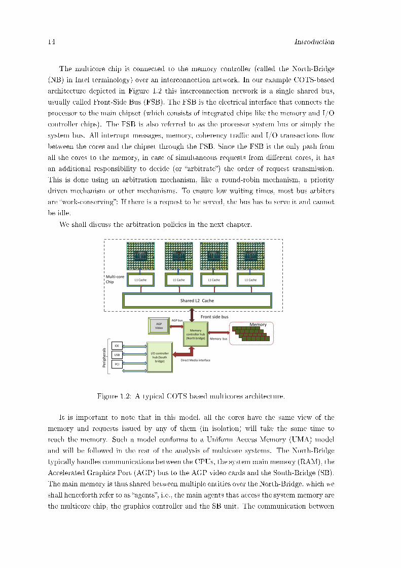
The multicore chip is connected to the memory controller (called the North-Bridge
(NB) in Intel terminology) over an interconnection network. In our example COTS-based
architecture depicted in Figure 1.2 this interconnection network is a single shared bus,
usually called Front-Side Bus (FSB). The FSB is the electrical interface that connects the
processor to the main chipset (which consists of integrated chips like the memory and I/O
controller chips). The FSB is also referred to as the processor system bus or simply the
system bus. All interrupt messages, memory, coherency tra�c and I/O transactions �ow
between the cores and the chipset through the FSB. Since the FSB is the only path from
all the cores to the memory, in case of simultaneous requests from di�erent cores, it has
an additional responsibility to decide (or �arbitrate�) the order of request transmission.
This is done using an arbitration mechanism, like a round-robin mechanism, a priority
driven mechanism or other mechanisms. To ensure low waiting times, most bus arbiters
are �work-conserving�: If there is a request to be served, the bus has to serve it and cannot
be idle.
We shall discuss the arbitration policies in the next chapter.
L1 Cache L1 Cache L1 Cache L1 Cache
Front side bus
Peri
ph
eral
s
Memory
controller hub (North bridge)
I/O controller
hub (South bridge)
IDE
USB
PCI
AGP Video
AGP bus
Direct Media interface
Memory bus
Shared L2 Cache
Multi-core Chip
Memory
Figure 1.2: A typical COTS-based multicores architecture.
It is important to note that in this model, all the cores have the same view of the
memory and requests issued by any of them (in isolation) will take the same time to
reach the memory. Such a model conforms to a Uniform Access Memory (UMA) model
and will be followed in the rest of the analysis of multicore systems. The North-Bridge
typically handles communications between the CPUs, the system main memory (RAM), the
Accelerated Graphics Port (AGP) bus to the AGP video cards and the South-Bridge (SB).
The main memory is thus shared between multiple entities over the North-Bridge, which we
shall henceforth refer to as �agents�, i.e., the main agents that access the system memory are
the multicore chip, the graphics controller and the SB unit. The communication between

1.4 Computing Platforms 15
the main memory and the other agents is handled by a memory controller and a memory
arbiter, both directly incorporated into the North-Bridge. Generally, a graphics controller
is connected to the NB (or is sometimes integrated into the NB as well depending on the
chipset design).
The South-Bridge, often referred to as the I/O Controller Hub, handles communica-
tion with the peripherals such as the hard-disk, keyboard, printer, etc., over a variety of
buses like the PCI) and PCI express. The peripherals can be connected in various ways
depending on the chipset design. Typically, the SB is connected to the NB via a Direct
Media Interface (DMI) channel. All the Direct memory access (DMA) tra�c (arising from
the peripherals) is also channeled through the south bridge.
Our multicore model: single shared bus with private caches only
After gaining an overview on the architecture of a multicore which clearly shows the
presence of shared resources like the shared bus, it is important to understand their impact
of execution behaviour of tasks hosted on them.
1.4.4 Contention for the shared hardware resources in multicore systems
In contrast to the uniprocessor design in which a single core had access to the cache,
the bus and the memory controller, the same low-level hardware resources are shared
amongst di�erent cores in a multicore system. Resources are mainly shared to minimize
cost, energy, and increase the performance, while conforming to the design parameters
of the end product, like the size, weight and power requirements. The problems in the
timing analysis of multicores can be mainly attributed to the interference on these shared
resources.
Consider a scenario in which there are several tasks assigned to each core in a multicore
system and all the cores are active. Under such a scenario, when a speci�c task su�ers
a cache miss and has to access the main memory over an interconnection network (like
the shared memory bus), its request may be blocked by the requests issued from tasks
executing on the other cores. Speci�cally, the core hosting that task is stalled, waiting
for the data to be fetched. As the number of cores that use the same front side bus
(FSB) increase, the tra�c on the FSB increases and this shared bus becomes the main
bottleneck. This means that the processor needs to stall for a longer time, waiting on the
data and hence more processor cycles are wasted. The extra delay incurred due to the
bus contention is non-negligible and hence the resulting execution time of a task can be
signi�cantly increased. It was shown by Zuravlev et.al [20] that FSB contention accounts
for as much as 60%- 80% of the performance variation that tasks experience on multicore
processors. Additionally, in some multicore systems, the caches are shared among the
cores; this further exacerbates the problem; tasks running simultaneously on two di�erent
cores may evict each other's cache lines, thereby increasing the number of cache misses,

16 Introduction
leading to additional requests to memory and adding to the tra�c on the shared bus.
Hence, any timing analysis for hard real-time systems in the context of multicore systems
cannot ignore the impact of the shared hardware resources. The requesters of a shared
resource may often access the resource at arbitrary times, which are di�cult to discern at
design time. As a result, di�erent access sequences may result in di�erent states of the
resource. The combination of di�erent resource-states and access patterns complicates the
analysis. The lack of spatial and temporal partitioning and the barely analyzable worst-
case timing behaviour of performance-enhancing features render the validation of claims
about the dependability and correct timing of applications on current powerful multi-cores
extremely di�cult to defend and prove.
1.4.5 From multicores to many-cores
Just as the technical community was getting used to the idea of multicore processors
in systems on chips (SoCs), advancements in semiconductor technology propelled chip
designers to further push the limits. On a casual note it may be said that, processor
cores are replacing transistors as the building blocks of the current computing hardware.
The multicore is becoming many-core; the number of processor cores closely coupled at the
hearts of SoCs is rising from 4 to 8, 16 and currently chips with 256 cores are already present
in the market. The Tile-Gx72 with 72 cores from Tilera [21], Kalray with 256 cores [22],
Epiphany with 64 cores from Adapteva, Intel Xeon co-processor [23] with 60 cores and
the 48-core Single-Chip-Cloud computer [24] are just some examples of such many-core
architectures. These systems, like Kalray's MPPA (Multi-Purpose Processor Array) have
been optimized to address the demand of high performance, low power embedded systems
and therefore these architectures must be analyzed. The next section provides an overview
of such an architecture.
1.5 Overview of a typical many core system
DDR3 Controller
DDR3 Controller
Smar
t NIC
Con
trolle
r
NetworkI/O
Two 10 Gb
&Two1Gb
UART x2USB x2JTAG
12C, SPI
PCIe 2.08 Lanes
PCIe 2.04 Lanes
Flexible I/O
Figure 1.3: Tilera architecture. (Diagram taken from [21])

1.5 Overview of a typical many core system 17
Figure 1.3 illustrates a many-core system based on the Tilera Platform. Without loss of
generality we shall discuss this particular platform to gain the basic understanding. As seen
in the �gure, the architecture of a many-core system is visibly di�erent from multicores,
considering the number of cores, the interconnection mechanism between di�erent cores
and the positioning of the peripherals and the memory controllers. It was seen that the
traditional shared bus/ring architecture (c.f. left plot of Figure 1.4) that serves as the
interconnect between the cores cannot not scale beyond some number of cores (typically
8 cores is the limit). The shared bus, instead becomes a bottleneck leading to substantial
increase in the access time to the o�-chip memory thereby o�setting the bene�ts of high
computing power provided by the cores. The increase in the number of cores forced a
shift in the earlier design paradigm towards a more scalable interconnection medium: the
Network on Chip architecture [25]. Longer wires connecting all the cores were replaced by
routed interconnects using switches. This design conforms to the distributed architecture,
while still being integrated on a single die.
Core1 Core2 Core3
Memory controller
Front-Side-Bus
Core4 Tile1 Tile2
Tile3
Memory controller
Tile4
Core3
switchNoC
cache
Traditional multicores architecture Massive multicores architecture
Figure 1.4: Multi-core vs. many-core architectures
Organization of the cores: One of the base principles of the many-core technology is
the division of the processing elements (cores) into �tiles� interconnected by a NoC. Each tile
is thus a basic modular unit, composed of a processor core, a private cache subsystem and a
network switch and these tiles are homogeneous across the entire chip. The tiles are laid out
in a two dimensional grid and the switch connects the tile to its neighboring tiles located
in the cardinal directions, thereby forming a 2D-mesh (c.f. right plot of Figure 1.4). The
NoC serves as a communication channel among the cores and between the cores and other
o�-chip subsystems, e.g. the main memory. The o�-chip subsystems like the peripherals
and the main memory are connected to the tiles on the periphery of the grid. Note that

18 Introduction
absence of a centralized single shared cache in this architecture, since it is distributed
across the tiles.
1.5.1 Contention of shared resources in NoC based many-cores
Route Computation
Input buffers
crossbar switch input 1
input 5
output 1
Output 5
Figure 1.5: Illustrating the switch, the physical links and bu�ers
Figure 1.5 gives some more details regarding the switch, in which the 5 physical links
incident on the input ports represent communication channels from each of the cardinal
directions connecting the given tile to its neighbors in the north, south, east and west
direction and a �fth link that facilitates the connection to the core present on that tile
itself. Similarly, the data leaves the switch from the output links. In this diagram we have
illustrated a single set of bu�ers which hold data from a given input port � in practice
there many be many bu�ers and therefore many virtual channels. The bu�ers act as storage
areas of �nite capacities or placeholders for data in transit, until the required output port
(and the corresponding output link) is busy. In this work, we assume a single virtual
channel. As seen in this diagram, the main shared resources in a NoC are these bu�ers
and the physical links.
At any given time, tasks running on di�erent cores may release packets over the network
independently and asynchronously. All the packets are transmitted over the same under-
lying interconnection network and share the available network resources. When several
packets try to access the same resource at the same time and if resources are insu�cient, it
leads to a contention � for example, a router in the network may be able to only serve one
packet and suspend the others based on some arbitration policy. Additionally, a packet
that is blocked at one link, can in-turn block other packets waiting on previous links and
the e�ects can cascade leading to a congested network, thereby causing a signi�cant delay
in the packet's traversal time. Thus the time to transmit a packet depends on the current
load of the network, which in-turn is determined by the number of packets generated by
the tasks executing on the other cores. Other factors like the routing mechanism employed
also impacts the traversal times as it in�uences the path taken by the packets to reach

1.6 Problems addressed in this thesis 19
their destination � this in-turn decides whether they would directly or indirectly block
the analyzed packet by contending for the same resources.
To summarize, the number of parameters contributing to the unpredictability combined
with the large number of cores poses a challenging problem to designers aiming to determine
an upper bound on the traversal time of a (message/memory/ IO) packet. This traversal
delay can be large and can increase the execution time of the task issuing these packets.
If real-time tasks are to be hosted on such many-core platforms, pre-assessing this delay
at design time is crucial. In this thesis we aim to compute such an upper bound which is
referred to as the worst-case traversal time (WCTT).
We are now equipped with the necessary background to understand the problems ad-
dressed in the thesis.
1.6 Problems addressed in this thesis
At the level of the processor, a task is generally a sequence of instructions which operate
on some data. Once the data is available to the processor, it performs the required compu-
tations. The instructions and data reside in some level of memory (L1 cache or L2 cache or
the main memory itself) within the memory hierarchy. Therefore, the total execution time
of a task can be demarcated as the computational phase and the communication phase,
between which an executing task keeps alternating. Then a simple way to compute the
execution time is given by,
Execution time = time for computation + time for communication
• The computational phase is the time during which the task consumes resources of
the processor or the on-core resources like access to the arithmetic logic units for
computations. In a multicore/manycore system, for a task that is assigned to a
processor, this component of the execution time is independent of the tasks executing
on the other cores.
• The communication phase represents the time to fetch the required instructions and
data from the memory, write the data back to memory or the time to communicate
between the cores. In this phase, the task consumes resources o� the chip, which
include the bandwidth available on the interconnection network which connects the
processing elements to the memory. In a multicore system, in which these o�-chip
resources are shared by the other cores, the communication delay is dependent on the
utilization of the same resources by tasks executing on the other cores. Similarly in a
many-core system the time to send or receive data across the shared interconnection
network is dependent on the data tra�c introduced by other cores.
Each data transfer constitutes a request for the interconnect mechanism (the shared bus
in multicores or the interconnected mesh network in many-cores). Consider task τi which

20 Introduction
needs Ci processing units (its WCET in isolation) and generates Ni requests. Assume that
request i needs wi units to be served, which implies that the core is stalled for the same
time, due to which the �nal execution time of the task in contention C ′i is given by
C ′i = Ci +
Ni∑i=1
wi (1.1)
In the broader context, the main aim of this thesis is to derive the delay incurred by the
executing task due to contention for the shared interconnect. Towards this aim the thesis,
explores related problems and subproblems, and we focus on three main areas:
1. Analysis of the impact of the shared bus on the execution time of a task in multicore
systems.
2. Analysis of the impact of the interconnection network on the traversal time of a
packet in many-core systems.
3. Analysis of multicore systems considering memory systems like Phase Change mem-
ory in which the read and write latencies di�er to a great extent.
We have enlisted the assumptions earlier, but will re-state them here for completeness.
1.6.1 Bus Contention Analysis of multicores
Problem statement: Given a multicore system, in which cores do not share cache space,
tasks are assigned apriori to all the cores and given the execution time of each task in
isolation, determine an upper bound on the increased execution of a task when it is run in
conjunction with other tasks co-executing on other cores. This analysis takes into con-
sideration the contention between co-executing tasks on all the cores for the single system
bus. The analysis assumes that tasks are sporadic, non-preemptive and the scheduler does
not allow tasks to migrate between cores. The main aim of the problem is to arrive at a
uni�ed framework for computing the WCET of a task, for any given arbitration mechanism
employed by the bus. The main problem is tackled by solving the following sub-problems:
1. To analyze the delay caused due to contention on the bus on a given task, a pre-
requisite is to analyze the memory tra�c injected by tasks executing on other cores.
Hence the �rst problem to be solved is modeling the memory access pattern of tasks
and deriving the maximum tra�c generated by the tasks in a given time interval.
2. Given the memory pro�le of every task on a core, the next problem to be solved
is deriving the maximum tra�c generated by the cores in a given time interval.
Being able to do so will provide an abstract interface that takes into consideration
all possible patterns of task arrivals and returns the maximum tra�c that can be
injected into the shared bus by any core in a given time interval.

1.6 Problems addressed in this thesis 21
3. A pre-requisite to analyze the maximum delay incurred by a request on the bus is
to understand the underlying arbitration mechanism. The order of servicing the
requests by the bus is based on its arbitration mechanism and the next step in the
analysis is modeling the availability of the bus� to demarcate the time intervals during
which the bus is busy handling tra�c (from the contending tasks) and the time at
which the bus is potentially available to serve the requests of the analyzed task.
4. The next problem is to develop a method of scheduling the requests (of the analyzed
task) on the available free bus slots with the objective of maximizing the waiting time
of each request and thereby computing the maximum delay that the task incurs. It
is very di�cult to derive at design time, the exact release time of every request and
we can only derive the number of requests that can be released over a period of time.
Give this coarse grain request distribution, we must be able to schedule requests in
a manner to generate the worst-case delay.
1.6.2 Network contention analysis of many-core systems
Problem statement: Given a many-core system in which the cores are arranged in a mesh
topology, and communicate with each other via an interconnection network, and data is
assembled into packets, compute an upper bound on the traversal time of the packet, con-
sidering the contention for the �nite links and bu�ers on the interconnection network. The
computed parameter is referred to as the worst-case traversal time (WCTT) for a NoC
based many-core system. The main problem is tackled by solving the constituent sub-
problems.
1. The �rst important problem is to characterize the application's �ow pattern and
compute the delay incurred by a packet in isolation.
2. A packet may incur delay at each intermediate router when contending with other
packets issued by other �ows. The next problem is to formulate a delay analysis by
considering the routing and switching mechanisms employed by the interconnection
network.
3. Given that packets may originate from di�erent �ows in di�erent orders, a method
to construct di�erent �ow sequences (scenarios) in order to generate that sequence
which can pose the maximum delay to the analyzed packet, is warranted.
4. To avoid an exhaustive enumeration during the generation of these scenarios, an
important concern is to reduce the number of investigated scenarios. This is done by
applying packet release constraints to the scenarios and pruning infeasible scenarios.
Other major design issue when many-core systems are concerned, is providing scalable
mechanisms that can cater to systems with large number of cores and can provide tight
bounds, e�ciently even when the network is heavily loaded.

22 Introduction
1.6.3 Analysis of Phase Change Memory (PCM) based multicores
A signi�cant part of the total delay incurred in serving requests of a given task, can be
attributed to the latency imposed by the memory sub-system. Unlike the timing analysis
of multicores where we consider a system for which the memory latencies for a read and
write request are the same, newer memory systems with asymmetric latencies like Phase
Change Memory (PCM) have been proposed. PCM is non-volatile, unlike Dynamic Ran-
dom Access Memory (DRAM), consumes lesser power and is sought after by embedded
system designers. We discuss more about PCM in detail in Chapter 5.
However, due to the intrinsic properties of PCM [26], the time to complete a read and
write operation di�ers greatly; completing a write operation may take upto 10 times the
time to complete a read request. If reads and writes are treated in the same manner by the
memory controller, it may lead to huge processor stall times, especially during very slow
write operations. To mitigate these delays, researchers have proposed di�erent scheduling
policies to be adopted by the memory controller: like prioritizing reads over writes in
order to reduce program stall times. It is interesting to explore such memory systems with
asymmetric read and write latencies and as a part of the thesis we also analyze such a
system for its temporal behaviour.
Problem statement: Given the WCET and the memory pro�le of a task in isolation,
compute the increase in the WCET when it runs in conjunction with other tasks deployed
on a multicore system in which Phase Change Memory (replaces Dynamic Random Access
Memory and) forms the main memory.
In addition to the analysis of the shared bus, the problem consists of analyzing the PCM
controller. This problem involves modeling the memory controller, computing the bus
availability for the analyzed task and then �nding a tight upper-bound on the cumulative
delay that memory requests may incur in the FSB and PCM controllers, considering that
the time to serve a write request is much higher than the time to service a read request.
We shall revisit this problem in detail in Chapter 5.
1.7 Motivation and Relevance of this work
The architecture of the execution platform decides if the timing analysis (static or mea-
surement based) is practically feasible at all and whether the most precise obtainable
results are precise enough. This in�uence of the architectural features has been of con-
cern to both the developers of timing-analysis tools and the consumers. With the shared
resource architectural paradigm supported by multicores, the problem has reached a new
level of severity. Multicores are thus not yet hard real-time ready � While multicores are
deployed in soft-real time embedded systems, their uptake in the hard real-time arena is
limited. Anecdotal evidence from practitioners suggests that multicores are being used in
hard real-time systems, with all but one core disabled, reducing it e�ectively to a single
core platform [27]. Hence, methods which could analyze the extra execution time due to
1.7 Motivation and Relevance of this work 23
contention on a shared bus would be valuable (much better than the current default alter-
native). The stark reality is that without addressing issues of shared resource contention,
highly robust hard real-time systems will not be deployable and the industry will be unable
to leverage the complete potential of emerging multicore systems.
1.7.1 The hardware solution: Building predictable multicores?
One solution would be to develop multi-core architectures that have features that make
them predictable and hence analyzable. Temporal and spatial isolation of components
should ideally be provided by the hardware itself. Spatial partitioning ensures that an
application in one partition is unable to change private data of another. Temporal parti-
tioning, on the other hand, guarantees that the timing characteristics of an application,
such as the worst-case execution time (WCET), are not a�ected by the execution of an
application in another partition. If present, these features reduce the time, e�ort and cost
involved in the analysis of these systems, since the temporal properties of each component
can be validated independently. For example, the use of partitioned (or partitionable)
caches, TDMA driven buses with guaranteed time allocations to cores and peripherals
would be advantageous. In these architectures, the resources would be temporally and
spatially partitioned making analysis easier.
The underlying problem however is that the safety-critical market is very small com-
pared with the consumer mass market (needing high performance systems) that is driving
chip development. The design paradigm of the current and future generation of processors
is inclined towards increasing the performance and as a consequence, there is no trac-
tion in the industry towards building predictable and analyzable systems. Development of
multi-cores based on a reference architecture dedicated to safety critical applications and
more amenable to certi�cation is likely to be prohibitively expensive unless cross domain
applications needing real-time support are large enough to force chip designers to build
analyzable systems. There is thus an opportunity to bring di�erent domains together,
aerospace, automotive, rail etc. to develop multi-core devices that are built from scratch
to be easily analyzable.
An alternative is to develop methodologies and toolsets that allow existing commercial
o�-the-shelf devices to be utilized in safety-critical applications. There is a need to satisfy
safety-requirements and provide time predictability. This will require further developments
in the underlying theoretical analysis of such systems and more importantly that the
developed tools to support this analysis, should be cost e�cient. Here there is a risk
of fragmentation across sectors due a wide spectrum of multi-core architectures being
developed. But we believe that unless the industry designs multicores which are real-time
friendly, developing methodologies to analyse the temporal properties is a crucial step.
As a logical step, it is of prime interest to understand the contribution of timing analysis
within the entire process.

24 Introduction
1.7.2 Missing link in the entire analysis process
While decades of active research have been spent in the timing analysis of uniprocessor
systems, the same cannot be said for multicores. Research is still in its nascent stages and
there are ample opportunities for improvement and �lling in the missing link in the analysis
cycle. To clarify, let us consider Figure 1.6 which depicts an iterative design/analysis
process suitable for tasks that do not migrate from one core to another at run-time. The
�rst step in this process involves modeling the number of cache misses that a given task
su�ers in isolation and computing its WCET. There is considerable research in this area
of WCET computation and the interested reader can refer to [10] for a compilation of
techniques to achieve this. The next step is assigning tasks on each core: this problem has
also been studied in detail and the existing research literature o�ers mature algorithms for
this particular activity [16]. Once tasks are assigned, we need to recompute the WCET
considering the contention on the shared resources. This is a key input to the next step
of �schedulability analysis�, after which we can ensure whether tasks meet their deadlines
� this is an open problem and the �missing link� in the entire design process. Hence it is
important and relevant to study this problem. Although some research has been carried
out, it has been done so with a lot of strong assumptions �however they do serve as the
building blocks in the �nal solution. We shall take a look in detail about the existing work
in the upcoming chapter which is totally dedicated to it. There are enough open venues
for improvement and this current research is aimed at addressing those issues to be able
to actually develop end-to-end solutions that will be accepted by the industry.
Assign tasks to processors
Perform schedulability analysis
Compute the WCET considering shared resource contention
Are task deadlines
met ?
No
Yes
Deploy tasks 1
Profile the cache behaviour and compute the
WCET of tasks in isolation
Figure 1.6: Flow Diagram for Analysis
The need for timing analysis is further driven by the facts that systems must be cer-
ti�ed prior to their deployment � it would be informative to understand the gist of the
1.7 Motivation and Relevance of this work 25
certi�cation process.
1.7.3 Certi�cation requirements and guidelines
A special class of hard real-time systems are safety-critical in nature. These systems
operate under strict timing requirements and may cause signi�cant damage or loss of life
and/or property if they do not operate in conformance with their pre-set functional and
non-functional speci�cations. Examples of these systems include �ight and tra�c control,
railway interchanges, nuclear facility control systems, medical equipment and implanted
devices. In order to ensure safe products, governments and international agencies took the
initiative in establishing certain certi�cation standards to regulate the quality of the �nal
products.
De�nition 11 (Certi�cation). �Certi�cation is the process of issuing a certi�cate to in-
dicate conformance with a standard, a set of guidelines, or some similar document.� �
Neil.R.Storey [28]
Certi�cation norms are applicable to processes and products. Di�erent safety standards
have been established across di�erent domains. Some of them are mentioned here:
• IEC 61508 is to ensure functional safety of electrical/electronic/programmable elec-
tronic safety-related (E/E/PE) systems.
• EN 50128 is to ensure safety norms in the railway industry
• RTCA/DO 178B and DO 254 for civil aircrafts in the avionics domain
• ISO 26262 is a functional safety standard, titled "Road vehicles � Functional safety"
targeted towards the automotive domain.
• IEC 61511, IEC 62061 are safety standards for the factory automation domain
Before safety critical real-time applications can be deployed on multicores, timing guaran-
tees must be ensured at design time and the entire system must be certi�ed. Researchers
have proposed various scheduling algorithms over the last decades, together with associ-
ated �schedulability analyses�, that enable certi�cation authorities to verify whether the
system will always ful�ll all its timing requirements at run-time. In practice, each and
every task of the system is assigned a �Safety Integrity Level� (SIL) re�ecting the level of
�criticality� of the task and the rigorousness of the certi�cation process varies according to
the SIL of the task under scrutiny. When deployed on the same multicore system, tasks of
di�erent SILs can co-exist and share some low-level hardware resources such as cores, cache
subsystems, communication buses and main memory. It is of chief importance to under-
stand that, unless these tasks of di�erent SILs are shown to be su�ciently independent, the
standards require that the hardware and software are developed at the highest SIL among
the SILs of all these tasks, which is very expensive. This requirement is clearly stated in

26 Introduction
the automotive domain (req. 7.4.2.3 of ISO 26262-4 [29]), as well as in the international
standard (req. 7.6.2.10 of IEC 61508 [30]). This is why substantial e�orts are put to (i)
render the tasks of a same SIL as independent and isolated as possible from the tasks with
di�erent SILs and (ii) upper-bound the impact that the execution of the tasks of a same
SIL may have on the execution behavior of the tasks of di�erent SILs, with the objective of
certifying each subset of tasks at its own SIL level.
As described earlier, by design constraints, complete isolation of tasks by partitioning
at the hardware level has its limit. In most multicores, the cores are typically connected
to a shared o�-chip main memory by a single shared communication channel (which does
not conform to the �total-isolation� paradigm). Sharing is either present at the level of the
caches or/and for the interconnection network or/and for the memory subsystem. Hence
in -line with the requirements, the work aims at providing upper bounds on the execution
time of tasks in the presence of a shared memory bus.
Additionally, to cater to these requirements, international standards also typically favor
simple and safe designs are recommended in [30] (Annex F, page 103). These include (i)
partitioned scheduling (tasks do not migrate when once assigned to a given core), (ii)
time-triggered architectures in which jobs are activated only at already known pre-set
time instants (iii) partitioned caches and cyclic scheduling algorithms (CSA) in which the
exact order of task arrivals is known at run time. In line with this requirements and the
complexity in analyzing data caches, the analysis in this work considers multicores with
partitioned caches. To summarize, analysis of multicores for their temporal behaviour is a
pre-requisite for certi�cation and is a motivating factor for this thesis.
1.7.4 Industry and Academic interest in multicores
Increased industry interest in adopting multicores for hard real-time systems is another
driving factor for this research. There has been clear evidence of a strong trend toward
using multicore processors in embedded systems that require hard real-time performance.
The industry is also increasingly collaborating with the academia to achieve this aim.
As a result, many related projects have been initiated at the European Union level,
some of them being:
1. RECOMP - Reduced Certi�cation Costs Using Trusted Multicore Platforms [31]
2. MERASA - Multicore Execution of Hard Real-Time Applications Supporting Ana-
lyzability [32]
3. ARAMiS - Automotive, Railway and Avionics Multicore Systems [33].
4. ACROSS - ARTEMIS CROSS-Domain Architecture [34]
5. CESar - Cost-e�cient methods and processes for safety relevant embedded sys-
tems [35]

1.7 Motivation and Relevance of this work 27
Given the gravity of the problem, researchers across the world have contributed in solving
di�erent parts of the entire problem. We shall present the state-of the art in the next
chapter. The above facts are instrumental in driving the need for analysis. But it is
also necessary to understand the hardness of the problem to be solved and the need for a
dedicated research e�ort in this direction.
1.7.5 Challenges in bus contention-aware timing analysis
To determine the WCET of a given task executing on a particular core considering the
contention on a shared memory involves an assessment of the incoming (request) tra�c
from the other cores. Firstly, the combination of parameters like the scheduling algorithm,
the memory pro�le of the co-scheduled tasks and their characteristics (like arrival patterns)
together increase the resulting search space, making design time analysis a non-trivial ex-
ercise. Secondly, memory requests from tasks generally do not follow a predictable pattern
which can be analyzed at design time - they are dependent on various factors including
the input to the task and whether or not the requested data was found in the cache.
It is di�cult to determine bounds for a shared bus employing a predictable arbitration
mechanism like TDMA, as the arrival of requests to the shared memory may not align in
time with the availability of the bus slot. With non-predictable bus arbitration policies,
the problem is further magni�ed. Thirdly, COTS-based buses are generally designed with
performance enhancing features (like pipelining requests, facilitating split transactions)
which e�ectively decrease the access latencies and reduce processor stall times �but this
complicated design makes it di�cult to analyze or adapt it to real-time systems, especially
in the absence of the required documentation (e.g details of the arbitration mechanisms
involved) and tunable interfaces (to change the existing arbitration policy). To summarize,
currently existing static analysis methods are restrictive, given the huge state space that
needs to be explored and measurement based methods need to consider the architectural
in�uences in extreme detail to obtain tight bounds on the obtained WCET values. Resolv-
ing the challenges of augmenting current designs and architectures to gain the bene�ts of
multicores for hard real-time systems can be daunting.
1.7.6 Contributions of this thesis
As seen above, the thesis addresses the constituent sub-problems of modeling the request
pro�les of the task and the core, modeling the bus availability and dealing with request
latencies imposed by the memory subsystem. While the major portion of the thesis focuses
on multicore platforms, a part of the thesis is also dedicated to the analysis of many-core
systems which communicate among themselves over a network. The main contributions of
this thesis are described here.
1. A basic requirement for computing the memory interference generated by a task is to
understand its memory access pattern. The thesis address this issue and a method for

28 Introduction
task pro�ling has been provided, which computes the maximum number of requests
a task can generate in a given time frame. We demonstrate using simulations that
the analysis provides tighter bounds than the state of the art techniques.
2. The next contribution is a method that enables to compute the maximum number
of requests that a core can issue, which takes into consideration the set of tasks
executing on that core. The method is novel in its kind to compute the per-task
pro�les and we also demonstrate using simulations that the analysis provides tighter
bounds than the state of the art techniques.
3. On the basis of the aforementioned methods, a uni�ed framework is proposed to
compute the increased execution time, which can handle di�erent arbitration bus
policies. We believe that this is the �rst kind which provides a common interface
to handle di�erent bus arbitration policies and computes the increased worst-case
execution time of a task by modeling the availability of the memory bus.
4. The thesis delves into the memory controller design and proposes a method to an-
alyze the increase in execution time for memory systems with asymmetric latencies
like Phase-change memory based systems. It takes into consideration the request
scheduling policies in the memory controller. This is the �rst work which analyses
memory systems with asymmetric latencies and considers the scheduling of requests
in the memory controller to derive the worst-case execution time.
5. The thesis also provides a method to analyze many-core systems in which the cores
organized as a grid, communicate over a network on chip infrastructure. A method
to compute the traversal time of a data packet is provided. The method identi�es
the sources of pessimism in the existing state of the art and improves upon it by
proposing techniques which not only provide tighter bounds but can also scale to
handle the contention when the network is heavily loaded �i.e. there is a large
amount of network tra�c.
Each of these contributions will be explained in detail in the forthcoming chapters.
1.8 Thesis Organization
The document is organized as a sequence of chapters. Chapter 2 explains the background
of timing analysis and details the earlier work carried out on timing analysis of multicores.
The key focus of Chapter 3 is to address the problem of deriving upper bounds on the
number of requests that a task can generate when run in isolation (per-task interference).
This memory pro�le is leveraged to compute naive upper bound on the interference from
each core (per-core interference). In chapter 4, a uni�ed framework for timing algorithms
which can be applied to di�erent arbitration mechanisms is established by de�ning certain
abstractions. At this point we deviate from analyzing the memory-bus and gain a deeper

1.8 Thesis Organization 29
insight into the memory subsystems with asymmetric read and write latencies. This is the
main focus of Chapter 5, which motivates the adoption of Phase Change Memory (PCM)
in embedded systems and analyses the temporal behaviour of tasks these multicores. After
analyzing multicores with a shared memory-bus, the thesis proceeds with the analysis of
many-core systems in which the cores communicate on a NoC. The communication channel
is designed as a mesh of links between cores which communicate over this network and the
data to be transmitted is encapsulated in packets. Chapter 6 explores this area in which
we identify the sources of contention on such a Network-On-Chip and study the worst-case
traversal time of a given packet. The work done in the thesis is discussed in the concluding
chapter 7 and the possible directions of research are laid out.

30 Introduction

Chapter 2
Background and Related work
We study history in order to intervene in the
course of history
Adolf von Harnack
In the previous chapter, we gave an overview of the problem of computing the increased
delay in the execution of a task due to the contention for shared resources like the shared
bus in a multicore system. This chapter is intended to provide the necessary background
before discussing the actual proposed solution. To facilitate this, the chapter is organized as
follows. Section 2.1 introduces the prevalent methods in timing analysis. Next, Section 2.2
describes the necessity of a newer analysis framework for multicore systems which takes
into consideration the impact of the shared resources and thereby introduces in detail these
shared resources. The work carried out by contemporary researchers towards solving this
problem has been summarized in Section 2.3. The chapter concludes in Section 2.4 which
enlists the avenues for improvement and further research in the given domain.
2.1 Timing Analysis
The computation of the parameters like the worst-case execution time is a part of the
process referred to as timing analysis. The aim of timing analysis is to give an estimate
for the time that a given program will take to execute under all feasible system states.
Although the work in this thesis is not focused on the computation of the worst case
execution time in isolation, the basics of timing analysis are presented here for the sake of
completeness.
2.1.1 Why is timing analysis required
By de�nition, hard real-time systems must satisfy timing constraints and must be validated
before deployment by a method called schedulability analysis. Analyzing a set of tasks for
schedulability veri�es if all the tasks will meet their deadlines when deployed on the target
31

32 Background and Related work
hardware. A vital input to this analysis requires safe and tight bounds on the execution
time of each task in the system. Di�erent methods have been proposed to compute such
estimates in uniprocessors and can be mainly classi�ed as static, measurement based and
hybrid techniques [36]. We will brie�y describe these methods in the following sub-sections.
2.1.2 Static Analysis
Static analysis methods analyze the task by constructing the program (task) �ow model,
the model of the target hardware and the inputs to the program. These techniques rely on
having a precisely accurate model of the timing behaviour of the target hardware, including
modeling features like pipelines, caches, memory, buses that a�ect the execution time of the
executing task [37]. The attempt is to derive safe bounds without actually executing the
program on the target hardware, while still considering the in�uence of the state changes
in the underlying hardware [38]. State changes could imply a cache line being evicted, a
pipeline being totally �ushed out, etc. The method computes the worst-case execution path
by considering constructing a control �ow-graph from a given program and considering each
of the paths in the graph. Loop bounds and other annotations provided to the analysis
tool help in facilitating the analysis. The timing analysis framework besides analyzing the
main program structure, is complemented by other modules like tools for cache analysis
and pipeline analysis that help in deriving estimates considering the speci�cs of the target
hardware. The modeling framework adopted by static analysis lends itself to formal proofs
which helps in establishing whether the obtained results are safe. Today, static WCET
tools are commercially available, including aiT [39] and Bound-T [40]. There also exists
several research prototypes, including Chronos [41], Heptane [42], and SWEET [43].
The safety and tightness bounds achieved by the static approaches are highly dependent
on the assumed abstract model of the target hardware. Earlier the embedded market
was traditionally dominated by simple and predictable processors, which were easy to
model and thereby derive safe and tight bounds. But within the increased computational
needs of modern embedded systems, designers have moved to complex processors which
are mainly designed for performance and not for predictability. In such a case, all the
intricacies contributing to unpredictability should be captured by the abstract model to
provide acceptable bounds. Hardware modeling relies on the chip manufacturers to publish
the details of the internal workings, which is generally not provided for di�erent reasons
(intellectual property and to be ahead in the competition). The models must be therefore
veri�ed to ensure that it indeed re�ects the target hardware. Failing to capture inherent
performance enhancing features may result in overestimations of the execution times and
the resulting bounds are not tight enough. Capturing all system states in a complex
machine may lead to unacceptably high analysis times. Additionally, building and verifying
the timing model for each processor variant is expensive, time consuming, and error prone.
This is re�ected in the high cost of commercial static analysis tools. Custom variants

2.1 Timing Analysis 33
and di�erent versions of processors often have subtly di�erent timing behaviors rendering
timing models either incorrect, or unavailable.
2.1.3 Measurement based techniques
The basic principle of this method follows the mantra that �The processor is the best
hardware model �. The program is executed on the actual hardware, in isolation and the
execution time is measured by instrumenting the code at di�erent points [44]. The major
task in this analysis is running the program to ensure coverage of all the paths by feeding-
in the representative set of inputs. Several thousands of program runs are carried out to
capture variations in execution time due to the �uctuation in system states during the
entire process. The maximum time recorded over all the runs, to which a safety margin is
added is then reported as the WCET of the program.
This method is clearly unsafe because it is di�cult to prove that path coverage ensures
the worst-case execution path has been indeed taken. Another issue is whether the extra
safety margin provably provides a safe bound, since it is based on some informed estimates
and cannot be acceptable for safety critical systems. A very high margin will result in
resource over-dimensioning, leading to very low utilization and while a small margin could
lead to an unsafe system. The integrity of the actual code to be deployed in the target
hardware is somehow depleted by the addition of the intrusive instrumentation code to
measure the time. Although, still a popular choice in the industry, measurement based
methods, have their drawbacks due to the aforementioned reasons.
2.1.4 Hybrid Approach
The hybrid approach, as the name suggests, assimilates the merits of the static analysis and
the measurement based approaches. The approach uses measurements to extract timing for
smaller program sections, and static analysis to deduce the �nal WCET estimate from these
timings. The approach identi�es certain �ow paths using static analysis and the execution
time of these �ow paths is measured on real hardware or by cycle-accurate simulators.
Finally, the information of the �ow paths is combined with techniques from the static
approach to determine the longest path. The advantage of the hybrid approach is that
it does not rely on complex abstract models of the hardware architecture. However, the
uncertainty of covering the worst-case behavior by the measurement remains since a safe
initial state and worst-case input can not be assumed in all cases. Moreover, instrumented
code is required which may not be allowed in particular certi�cation. Example tools include
Rapitime [37] and MTime.
Given that these tools exist for uniprocessors, an interesting question is whether they
can be used for multicore analysis. The next section explains the need for a newer analysis
framework.
34 Background and Related work
2.2 Timing Analysis: Uniprocessors to Multicore systems
Most of the improvements in performance in uniprocessors is achieved by employing meth-
ods like pipelining, branch prediction, and out-of-order execution in the processor and
o�-chip caches. While caches are used to bridge the gap between processor speed and the
access time of main memory, pipelines enable acceleration by overlapping the executions of
di�erent instructions. Control speculation (out of order execution, branch predictions) is
used to avoid pipeline stalls caused by conditional jumps. These on-chip subsystems were
the main focus of the uniprocessor timing analysis and a detailed survey of the work in
this domain is presented in [10]. As a result of the extensive research, WCET analyzers
which are adopted by the industry are already available for uniprocessors. Examples are
aiT [10, 39], SWEET [10, 43] and RAPITime [10, 37].
2.2.1 Need for a new analysis paradigm
The key di�erentiator between multicores and their predecessors, the uniprocessors has
not been in the basic processor design, but the packaging of these multiple cores, sharing
the same hardware resources. The number of cores have been increased to boost the
computing power, but the same resources that were dedicated to a uniprocessor systems
are now shared by many cores in the case of multicores. The impact of sharing leads
to considerable variations in the execution time of tasks, which cannot be overlooked.
Although the earlier timing analysis tools developed for uniprocessors have robust methods
to provide the WCET of tasks in isolation, the absence of an analysis of the impact of shared
resources has become a very evident drawback in these tools, warranting an additional
analysis framework to provide a holistic solution.
While the WCET of task in isolation is an inherent property of a task, the WCET
of a task when co-executing with other tasks largely depends on their access patterns
to the shared memory. Therefore a task τi running on Core πp executing with task τj
on Core πq, sharing the same memory via a shared bus may have completed at time
say Ci1, whereas the same task τi on Core πp that executes concurrently with task τk
assigned to Core πq may complete at a di�erent time Ci2 (6= Ci1). This change in execution
behaviour must be captured by the newer analysis framework. As a logical progression,
the current research for analyzing the temporal behaviour of tasks in multicores is now
inclined towards studying the impact of these shared resources. To summarize, while
there is enough research available on computing the WCET of a task in isolation, with
all resources dedicated to it for uniprocessors, it cannot be adopted as is and will need to
factor-in the impact of the extra delay due to contention on the shared resources.
As described earlier, the main focus is of this work is the analysis of the shared resources,
namely shared bus, caches and the memory. We shall next focus on each of this.

2.2 Timing Analysis: Uniprocessors to Multicore systems 35
2.2.2 Background on the system bus (front side bus)
A bus in general refers to a bi-directional communication channel that transfers data be-
tween components inside a computer, or between computers. This expression covers all
related hardware components (wire, optical �ber, etc.) and software, including communi-
cation protocols [45].
In multicore systems, the system bus or the front-side bus (FSB in the Intel's terminol-
ogy) provides the communication channel between the processing units and the memory.
All interrupt messages, memory, coherency tra�c and I/O transactions �ow between the
cores and the chipset through the system bus. It is important to note that we do not deal
with the I/O bus which connects with peripherals to the memory controller.
Control bus
Áddress bus
´Data bus
Memory controller
Memory
Front side bus Memory bus
Multicore chip
Figure 2.1: System bus (Front side bus)
Figure 2.1 illustrates the positioning of the FSB w.r.t the processing chip and the
memory. Buses, in general consist of separate channels to transmit the data and the
address of the memory location from where data is to be fetched from or written to. These
channels are accordingly called the data bus and the address bus. Additionally there is
a control bus which is used to transmit control signals across communicating units. The
number of bits transmitted by the data bus (say 32 bits or 64 bits) represents its width.
If the size of the data exceeds the bus-width, it is sent in multiple transfers. The size
(or width) of the address bus indicates the maximum amount of memory a processor can
address. Another property of the bus is the speed (clock frequency) at which it transfers
data [46], expressed as number of cycles per second or Hertz (Hz). Bus clock speeds of 400
MHz, 533 MHz, 667 MHz, 800 MHz, 1066 MHz, or 1333 MHz are very common in modern
processors.
Another important term associated with the bus is the bandwidth or maximum the-
oretical throughput which represents the amount of data it can transfer per time unit.
Bandwidth = width× clock frequency× transfers per cycle
The bandwidth is thus determined by the product of the width of its data path, its clock
frequency (cycles per second) and the number of data transfers it performs per clock
cycle [46]. For example, a 64-bit (8-byte) wide FSB operating at a frequency of 100 MHz
36 Background and Related work
that performs 4 transfers per cycle has a bandwidth of 3200 megabytes per second (MB/s).
This value is computed as 8B ×100 MHz ×4 transfers/cycle = 3200 MB/s.
2.2.3 Bus Transactions
Buses operate on messages and transactions. We describe these terms here.
• Message: A message is a logical unit of information; for example, a write message
contains a memory address to which the data must be written, control signals and
the data to be written. A message requires a number of clock cycles to be sent from
sender to receiver over the bus.
• Transaction: A transaction consists of a sequence of messages which together form a
transaction. For example, a read transaction consists of a memory read message con-
taining the address which must be read and a corresponding reply with the requested
data.
Bus transactions can be carried out in several ways:
1. Atomic bus transaction: The simplest way to perform a non-split or atomic transac-
tion is to implement a shared bus with an atomic bus protocol. In such a mechanism
a transaction is modeled as an indivisible request-reply pair. A given request can-
not be serviced before the bus transmits the response to the prior request. While
this is simple to implement, the bus is underutilized and there is a performance hit
considering that the next request is served only after the response to the previous
request is obtained. In order to improve the throughput of the bus, designers have
implemented mechanisms like pipelining and split transactions [47].
2. Bus pipelining: A bus transaction is divided into multiple stages (like arbitration, bus
request, error reporting, snoop, reply, data). For example, the control bus handles
sub-operations like the arbitration, request, error reporting , while the data bus is
responsible for transmitting the data written to or read from memory. Since each
part of the transaction does not use the same bus signals, a pipelining mechanism
which entails overlapping multiple transactions that do not use the bus components
simultaneously, is employed to increase the throughput (number of requests served
in a given time). For example, the data bus is not used during address cycle, and
address bus is not really needed during data cycles. Then the utilization of the
bus can be improved by overlapping the address cycle of each transaction with data
cycles of previous transaction. In general, any two phases of a transaction that use
a separate set of physical signals (wires) can be pipelined.
3. In a split-transaction bus, a transaction is demarcated into two sub-transactions: a
request transaction and a reply transaction. Both transactions (requests and replies)
have to compete for the bus by arbitration. In such a mechanism, when a core places
2.2 Timing Analysis: Uniprocessors to Multicore systems 37
a memory request on the bus, that core then immediately releases the bus, so that
other requesters can use the bus while the memory request is in the process of being
served. When the memory request is completed, the memory module involved will
then acquire the bus, place the results on the bus (the read value in the case of a read
request, an acknowledgment in the case of a write request), and also place on the
bus the identity number of the core that made that request. The memory response
is tagged with the identity of the core and the bus controller redirects the response
to the corresponding core.
A pipelined bus provides responses in the order in which the requests were sent, while
with split transaction buses, responses may be served in an order which does not match
the order of requests issued. The advantage of a split-transaction bus over a pipelined bus
is that a low-latency response does not have to wait for a high latency response to a prior
request. The disadvantage (of a split transaction bus) is that both the request and the
response phases must arbitrate for the bus and must be tagged with the identity of the
requester. An atomic bus and a pipeline bus, by design are examples of in-order buses,
while a split-transaction bus is an example of an out-of order bus.
We assume a shared-bus with an in-order, atomic transaction protocol
Another way to minimize the stall times in the processor is by a hardware initiated
prefetching mechanism.
Hardware Prefetching Modern processors also provide hardware pre-fetching as a
memory-latency hiding mechanism. The prefetcher predicts the next memory addresses
to be accessed and pro-actively fetch this data from the main memory to the last-level
caches based on observing memory access patterns. Processors based on the Intel NetBurst
micro-architecture provide two prefetch mechanisms through the BIOS: Automatic hard-
ware prefetch and Adjacent Cache Line Prefetch [48]. The Automatic hardware prefetcher
prefetches streams of data and instructions from memory into the uni�ed L2 cache on
detecting successive L2 cache misses and a stride in the access pattern, as in accessing
successive elements in an array, leveraging the property of locality of reference in program
access patterns. The Adjacent Cache-Line Prefetch mechanism, when enabled through the
BIOS, always fetches two 64-byte cache lines, irrespective of whether the additional cache
line has been requested or not. However, there are two main problems when real- time
tasks are concerned. Firstly, the prefetch requests consume bus bandwidth and may delay
important demand requests issued by real-time tasks. Secondly they can lead to cache
pollution by prefetching lines that are not required by the tasks and evicting re-usable
cache lines belonging to real-time tasks. When enabled, this OS-transparent prefetching
can run in the background at arbitrary times, resulting in variations experienced by the
currently executing tasks. Many processors, e.g. from Intel, allow programmers to disable

38 Background and Related work
this feature (see [48]) and it is important to do so to minimize the variations in temporal
behavior.
In this work, we assume that hardware prefetching is disabled
2.2.4 Contention on the system bus
As described earlier, multiple cores access the main memory via a shared bus. This often
leads to contention on this shared channel, which results in an increase of the response
time of the tasks. Analyzing this increased response time, considering the contention on
the shared bus, is challenging on COTS-based systems mainly because:
• bus arbitration protocols are often undocumented and the implementation of arbi-
tration protocols is hidden
• the exact instants at which the shared bus is accessed by the tasks are not explicitly
controlled by the operating system scheduler; they are instead a result of cache misses,
TLB misses, coherency tra�c, etc.
• requests are not tagged with any task priority information and thus, although the
cores may enforce this prioritization and give preferential access to tasks with higher
priorities, the bus may re-order the memory requests based on its internal priori-
tization and request scheduling mechanisms. As a consequence, requests issued by
higher-priority tasks may be served later than those from lower-priority tasks.
To complicate matters, the FSB in modern processors may be an out-of-order bus (e.g.,
the Intel Itanium Processor Family) and employ other performance-enhancing mechanisms,
including split transactions and pipelining. If pipelined buses are employed, the time for
several bus transactions is not tightly bounded by simply adding the execution times of
the individual transactions, since the phases within a transaction (typically arbitration,
request, error, snoop, response, optional data phase) may be overlapped. For example, the
Intel 4 Chipset Family boards [19] have a 12-deep in-order queue to support up to twelve
outstanding pipelined requests on the FSB. In principle, the extra overhead due to the FSB
is attributed to two main factors: the communication delay on the bus, which depends on
the speed and data width of the bus and the time until a free slot is available on the bus.
If requests are served in-order, then the �rst overhead can be upper bounded, since the
required parameters are generally documented. The second factor is largely dependent on
the bus arbitration mechanism which we shall explore next. The shared-bus architecture
is appealing to chip designers given its simple topology, low area cost and the ease of
implementation. The disadvantages of shared bus architecture are larger load per data bus
line, longer delay for data transfer, larger energy consumption, and lower bandwidth [49].
When multiple requesters compete to access a common resource, like a shared memory,
a networking switch fabric or a computational element (processor), an arbiter is required

2.2 Timing Analysis: Uniprocessors to Multicore systems 39
to determine the order in which the shared resource is granted access to the requesters. In
the next part, we will look at di�erent arbitration mechanisms.
2.2.5 Bus arbitration policies
Associated with every bus is a protocol that de�nes the order of access by the devices
attached to the bus (arbitration), the rules that the attached devices must follow to com-
municate over the bus (handshaking), and the signals associated with the various bus lines.
Bus arbitration is based upon devices being classi�ed as either master devices or requesters
(devices that can initiate a bus transaction) or slave devices (devices which can only gain
access to a bus in response to a master device's request like the bus controller). In the case
of a shared bus, the bus arbiter controls the access of multiple cores to the shared memory.
In the case of simultaneous requests for access to the bus, the arbiter resolves these access
con�icts by serializing the requests from the di�erent cores according to a set of rules which
constitute the arbitration policy. This arbiter can grant the bus to a requester for a �xed
number of bus slots, where each bus slot may span over a number of bus cycles.
Arbitration policies can be primarily categorized as dynamic and static arbitration
policies. A dynamic arbitration policy resolves simultaneous accesses at runtime, while a
static arbitration policy strictly de�nes the access pattern at design time. Fixed priority
arbiters, �rst-in �rst-out (FIFO) and round-robin arbiters are examples of the dynamic
arbitration policy, while Time Division Multiplexing (TDM) is a classical example of a
static arbitration policy. Fixed-priority arbitration may be used in platforms with diverse
response time requirements, TDM in platforms that require robust partitioning between
applications, and round robin when a simple notion of fairness between cores is required.
In the �xed-priority arbitration policy, each requester is assigned a unique priority, and
the grant is given to the active requester with the highest priority. The key shortcoming of
priority arbiters is that, if high priority tasks are highly memory intensive, then requests
from lower priority tasks may starve and may need to wait inde�nitely before receiving a
grant to access the bus.
A round-robin arbiter on the other hand, is a fair scheme and allows every active
requester to access the bus in-order. It is also called the rotating priority scheme, in which
the requester that is most recently granted the bus receives the lowest priority, while the
next requester receives the highest priority. The basic algorithm dictates that once a
requester has been served it would �go around� to the end of the pending request queue
and be the last to be served again.
A specialized version called the weighted round-robin arbiter �rst assigns di�erent
weights to requesters and grants them bus cycles proportional to their weights; a higher
weight means a higher number of cycles. This weight assignment is done repeatedly after
N cycles. For example, if three requesters are assigned weights 1,2 and 3, then they get
N/6, 2N/6 and 3N/6 cycles every N cycles periodically whenever they access the bus [49].

40 Background and Related work
In the First-in First-out arbitration scheme, a queue is maintained that stores a list
of master devices (or processor cores) that are ready to use the bus in the order of bus
requests. The access to the bus is thus serialized by a mechanism in which the cores that
had to transmit earliest are placed at the front of the queue while later requesters are
added at the end of the queue. One main drawback is the possibility of the arbiter not
intervening if a single master at the front of the queue maintains control of the bus, never
completing and not allowing other masters to access the bus.
A Time Division Multiplexing arbiter works by periodically repeating a schedule, or
frame, with �xed size. Each core is allocated a pre-computed number of slots in the frame
at design time. Requests from a core are only scheduled during slots allocated to that
core. Empty slots or slots allocated to other cores without pending requests are hence
not utilized. This type of policy makes the timing behavior of memory requests of tasks
scheduled on di�erent cores completely independent.
TDM arbitration, is therefore by design a composable and predictable arbitration
scheme; predictable since the maximum time of access to a resource is bounded and com-
posable because the access time is independent of other requesters. The round robin arbiter
on the other hand is predictable, as the maximum time of access to a resource is bounded,
but not composable, since the access to the shared resource (the bus here) depends on
the number of other active requesters. A �xed priority arbiter, is neither predictable nor
composable as the time for access to a resource cannot be upper bounded until there is
su�cient knowledge about the access patterns of the higher priority requesters.
Some of the bus standards for the system buses include (i) Advanced Microcontroller
Bus Architecture standard from ARM which de�nes the Advanced System Bus in their
earlier processors and the AHB (Advanced High-performance Bus) in the more recent
versions (ii) CoreConnect from IBM which it refers to as Processor Local Bus and (iii) the
Front Side bus from Intel. The buses from ARM and IBM also apply for System-on-chip
designs where the main memory and the cores reside on a single chip.
Bus Topology Multiple cores can be connected to each other in di�erent ways as seen
in Figure 2.2.
In this thesis, we analyze cores connected by a shared bus and mesh topologies.
After studying the basics of the shared bus, let us understand another resource, which
plays a vital role in execution time of the task: the cache.
2.2.6 Caches and cache analysis
In most of the existing multicores, the large gap between the core speed and the memory is
bridged by keeping the most frequently accessed data closer to the cores. In simple terms
a cache is a storage area which bu�ers the most recent memory accesses. In the overall

2.2 Timing Analysis: Uniprocessors to Multicore systems 41
(a) Cores connected using ashared bus
(b) Cores connected in a ring
(c) Cores connected in amesh topology
Figure 2.2: Bus Topologies
system architecture, caches are organized as stacked hierarchy; the CPU is at the top,
followed by layers of one or more caches and then the main memory. In this multi-level
hierarchy, caches are quanti�ed by their level. The cache closest to the CPU is called level
one, L1 for short� caches increase in level until the main memory is reached.
Cache Line A cache line or cache block is the smallest unit of memory that can be
transferred to or from a cache. The essential elements that quantify a cache are called the
read and write line widths. These signify the minimum amount of data the cache must
read or write from the memory or cache below it. Frequently, these quantities are the
same, so caches often are quanti�ed simply by the line width.
Cache Size The next property that quanti�es a cache is its size. This number is an
indication of how much data could be stored in the cache.
Inclusive and Exclusive caches A multilevel cache can be either inclusive or exclusive.
In an exclusive cache, a particular cache line may be present in exactly one of the cache
levels. Alternatively in an inclusive cache, the cache line may be present simultaneously in
more than one level of the cache.
In this work, we make no assumptions on the inclusivity
42 Background and Related work
Write policy The write policy determines the time at which the modi�ed cache line is
written back into memory. In a write-through cache the main memory is made consistent
with the modi�cations in the cache line immediately after a cache-line write. In contrast,
in a write-back cache the process of updating the main memory is de�ered to a later time,
until the given cache line is evicted. The status of the cache line is however marked dirty
in order to signal that the memory copy and the cache-copy are not coherent with each
other.
In this work, we assume write-through caches
Cache associativity In general, caches consist of several �sets�, each of which consists
of k �ways�: k is called the �associativity�, and is usually 1, 2, 4, 8 and is higher (16 way
is not uncommon these days) in modern day processors. Caches are called direct mapped
for k = 1, and set associative otherwise. Each way can hold one line from memory. The
entries stored in the caches are not single words but, instead, �lines� of several contiguous
words. In early caches these lines were 32 bytes long; now the norm is 64 bytes � and the
terminology used is that the cache line size is 64 bytes. The relationship of all these values
to the cache size is
Cache Size = Cache line size× associativity× number of sets
Thus a cache with associativity 8 with a cache line of 64 bytes containing 512 cache sets
has cache size of 256k bytes.
Cache replacement policies: On cache updates, the replacement strategy determines
the cache-way which must be evicted to store the current cache-line. Common strategies
for replacement are pseudo-least recently used (PLRU), LRU (in older processors), �rst-in
�rst-out (FIFO) and random replacement. LRU replacement conceptually maintains a
queue of length k for each cache set, where k is the cache associativity [50]. If an element
(a memory block) is accessed that is not in cache (a miss), it is placed at the front of
the queue. The last element of the queue, the LRU element, is then removed if the set is
full. At a cache hit, the element is moved from its position in the queue to the front, in
this respect, treating hits and misses equally. LRU replacement is used in the Freescale
PPC603E core and the MIPS 24 K/34 K. FIFO cache sets can also be seen as queues: New
elements are inserted at the front, evicting elements at the end of the queue. In contrast
to LRU, hits do not change the queue. FIFO is used in the Intel XScale and some ARM9
and ARM11-based processors. PLRU is a tree-based approximation of the LRU policy.
It arranges the cache lines at the leaves of a tree with (k − 1) �tree bits� pointing to the
line to be replaced next (for an in-detail explanation of PLRU, consider [51]). It is used
in the PowerPC 75x and the Intel Pentium II, Pentium III and Pentium IV processors.
The precision and e�ciency of cache analysis strongly depend on the predictability of the

2.2 Timing Analysis: Uniprocessors to Multicore systems 43
employed replacement policy. The LRU replacement policy is most predictable of the
known policies. Employing other policies, like PLRU or FIFO yield less precise WCET
bounds, because fewer memory accesses can be precisely classi�ed.
In this work, we make no assumptions on the replacement policy
2.2.7 Problem with shared Cache Analysis
An important step in timing analysis of a given task is its cache analysis, which tries
to classify memory accesses as hits or misses. Memory accesses that cannot be safely
classi�ed as a hit or a miss have to be conservatively accounted for by considering both
possibilities. Apart from the high associativity and the write policies, the predictability
of cache behavior is largely in�uenced by the replacement policy, which is usually pseudo
least-recently used (PLRU) in many multicore platforms from Intel and In�neon. The
impact of these replacement policies on predictability has been presented in [51].
In unicore systems, the problem of sharing the cache among tasks that could pre-empt
each other (pre-emptive scheduling) on the same core is intricate [52] and the analysis to
compute this extra cache-related pre-emption delay is already non-trivial. The problem
is further exacerbated in multi-cores when co-executing tasks on other cores share and
contend for the same cache lines, thereby increasing the possibility of cache-line evictions.
Although the higher capacity of the caches was provided to decrease the accesses to main
memory and thus reduce the stall time of executing tasks, non-ownership of these shared
cache lines by the cores can lead to unregulated cache evictions and cache thrashing.
This defeats the very purpose of providing a larger cache as it leads to increased memory
requests. Additionally, bounding the number of memory requests that a particular task
may generate in an interval is challenging at design time, since memory requests from
tasks do not arrive periodically and the order in which tasks are executed is dependent on
the on-core scheduling policy. In fact, the number of varying patterns of task arrivals on
other cores, replaceable cache lines and memory request patterns result in a combinatorial
explosion of possibilities. As seen above, given the complexity of the caches present in
modern day processors, it is extremely challenging to derive tight estimates for shared
caches. In [53], the authors clearly demonstrate that cache partitioning provides an
e�ective means of bounding and controlling interference patterns in shared cache on an
multicore system. In particular, WCETs can be bounded and controlled much more tightly
when the cache is partitioned. This allows system designers to set relatively tight, yet safe,
execution time budgets, thereby maximizing system utilization. The impact on bounding
WCETs is more pronounced when the working set size of the task �ts within the cache
partition assigned to the core. That said given that embedded, real-time applications tend
to have relatively small working set sizes, it is expected that cache partitioning will bene�t
most applications. In lieu of these facts, it may be said that hard real-time systems are
more likely to be developed on processors with private caches or by either disabling or
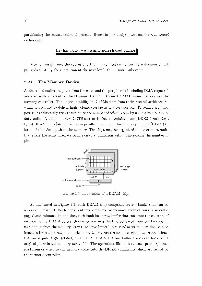
44 Background and Related work
partitioning the shared cache, if present. Hence in our analysis we consider non-shared
caches only.
In this work, we assume non-shared caches
After an insight into the caches and the interconnection network, the document next
proceeds to study the contention at the next level: the memory sub-system.
2.2.8 The Memory Device
As described earlier, requests from the cores and the peripherals (including DMA requests)
are eventually directed to the Dynamic Random Access (DRAM) main memory via the
memory controller. The unpredictability in DRAMs stem from their internal architecture,
which is designed to deliver high volume storage at low cost per bit. To reduce area and
power, it additionally tries to minimize the number of o�-chip pins by using a bi-directional
data path. A contemporary COTS-system typically contains many DDR3 (Dual Data
Rate) DRAM chips [54] connected in parallel on a dual in-line memory module (DIMM) to
form a 64-bit data path to the memory. The chips may be organized in one or more ranks
that share the same interface to increase its utilization without increasing the number of
pins.
row buffer
activate
(open)
precharge
(close)
row address
column address I/O
data
bank
s
writeread
Figure 2.3: Illustration of a DRAM chip.
As illustrated in Figure 2.3, each DRAM chip comprises several banks that can be
accessed in parallel. Each bank contains a matrix-like memory array of rows (also called
pages) and columns. In addition, each bank has a row bu�er that can store the contents of
one row. On a DRAM access, the target row must �rst be activated (opened) by copying
its contents from the memory array to the row bu�er before read or write operations can be
issued to the word-sized column elements. Once there are no more read or write operations,
the row is precharged (closed) and the contents of the row bu�er are copied back to its
original place in the memory array [55]. The operations like activate row, precharge row,
read from or write to the memory constitute the DRAM commands which are issued by
the memory controller.

2.2 Timing Analysis: Uniprocessors to Multicore systems 45
The DRAM architecture makes the response time of memory requests and the provided
bandwidth highly variable for three reasons:
1. a request targeting an open row can be served immediately, while it otherwise needs
the current row to be closed and the required row to be opened (details follow in the
next sub-section),
2. the bi-directional data path requires several cycles to switch from read to write and
vice versa,
3. to prevent data loss, the memory must occasionally be refreshed before executing the
next request and the added refresh time may be longer than the time to serve the
request itself.
The impact of these three factors may cause the execution time of e.g. a 64 Byte memory
request to vary by an order of magnitude from a few clock cycles to a few tens of cycles.
DRAM memories can hence be considered highly unpredictable resources by nature and
are challenging to work with in the context of real-time systems.
2.2.9 Memory Controller
The memory controller connects the system to the o�-chip DRAM and is responsible for
scheduling memory accesses according to the system requirements. In a COTS system,
the memory controller achieves this by maximizing the average bandwidth and minimizing
the average latency, while limiting power consumption. This typically implies maximizing
the utilization of the data path, possibly subject to di�erent priorities of memory streams,
when there are pending requests and make e�cient use of power-down modes in the memory
device when there is idle time. Overall, there are three factors that a�ect the response
time of memory requests in the memory controller: i) the page policy, ii) the scheduling
algorithm, and iii) the power-management policy. We proceed by discussing each of these
in turn.
Page policy The page policy determines when precharge commands should be issued
by the memory controller [56]. Currently, there are two prevalent page policies: open page
and close page.
The open-page policy tries to improve the average performance of the memory controller
by exploiting locality among memory requests. This is achieved by speculatively keeping
activated rows open after memory accesses, hoping that the following requests to the banks
target the same rows, thereby eliminating the latency and power overhead of activating
and precharging the banks [55]. The drawback of this approach is a latency penalty in case
the following request requires di�erent rows in the banks, as this results in precharging and
activation while the request is stalling. The open-page policy works well in case there is

46 Background and Related work
su�cient locality in the memory stream to generate enough row hits to make a net gain in
average performance despite this penalty.
In contrast to the open-page policy, the close-page policy always closes the active rows
immediately after each memory access to minimize the overhead of opening another row
in the same bank. This policy is bene�cial when there is not su�cient locality within
the memory stream of an application, or when locality is destroyed when memory streams
from di�erent applications are multiplexed in the memory controller to access the single
o�-chip memory. This policy is typically favored by memory controllers for hard real-time
systems [57, 58, 59], since they are unable to guarantee any locality in the worst case due
to �ne-grained sharing of the memory, and hence prefer to reduce the miss penalty.
Hybrid policies that combine properties of open- and close-page policies have also been
proposed. To improve performance of their systems, Intel proposed an adaptive page
policy [60] that dynamically switches between open- and close-page policies based on the
locality in the memory streams. In the context of real-time systems, a conservative open-
page policy [61] has been proposed. The key idea is to partially exploit locality by keeping
active rows open as long as possible without negatively impacting the worst-case response
time of memory requests. This approach works well if there is locality in the memory
tra�c and if requests arrive close enough together to enable row hits to be detected early.
In our analysis, we do not delve deeply into the memory subsystem. Any page policy
that facilitates the computation of upper bounds on the time for a memory access can be
modeled in our analysis.
We make no speci�c assumptions on the page policies
Scheduling algorithm The memory scheduler is responsible for ordering incoming
memory requests and generating DRAM commands (like activate row, precharge row,
read row) that are scheduled according to the timing constraints of the memory. This may
involve a two-level scheduler, one level for memory requests and a second one for DRAM
commands, although it is possible to integrate the two. The memory scheduler is often
very dynamic and uses information about the memory state when scheduling to improve
average bandwidth or reduce average latency. Optimizing bandwidth may involve prefer-
ring requests that target an open row in a bank [62, 56, 63], requests that �t with the
current direction of the data path [64, 65, 66], or a combination of the two [67, 68, 69]. Ex-
ample mechanisms that reduce average latencies is to prefer reads over writes [63], which is
bene�cial if reads are blocking while writes are posted, or let high-priority memory clients
preempt lower priority clients [69]. Another technique to reduce latency is presented in [62]
that schedules memory bursts belonging to the same requests simultaneously thereby un-
blocking the stalling processor earlier. It is also proposed in [70] to try to schedule refresh
operations during idle cycle cycles when there are no requests pending or even executing
multiple refresh operations in sequence when idle to amortize overhead [71]. The problem
2.2 Timing Analysis: Uniprocessors to Multicore systems 47
with these dynamic memory schedulers is that the interactions between the request and
command schedulers are complex, especially in the presence of the aforementioned mech-
anisms. Thus, neither of the above memory controllers provide bounds on bandwidth or
latency, making them di�cult to use in the real-time context.
Power policies DRAM memories have several power-down modes [54], e.g. power-down
with fast exit, power-down with slow exit, and self-refresh. These modes have increasingly
large transition times in and out of the low-power state, while the current through the
memory is decreasing, thus o�ering di�erent trade-o�s depending on the length of the idle
periods and the maximum tolerable wake-up penalty. A consequence of the sometimes
substantial wake-up penalties is that the worst-case memory latency does not happen
when the memory controller is maximally loaded, but when there are sudden bursts of
memory requests while the memory is in self-refresh. Determining the critical instance
for the memory controller may hence be di�cult without information about the power-
management policy, further complicating the process of estimating memory latencies with
both analytical and measurement-based techniques.
Summary The time to serve a memory request is highly variable and strongly depends
on the architecture of the memory itself, as well and the scheduling algorithm and page-
and power policies used in the memory controller. All this information is generally not
divulged for COTS systems, hence it is di�cult to obtain an accurate estimate of the
memory latency. The memory controller may o�er con�guration options to disable dynamic
features, such as reordering mechanisms, which makes the scheduler easier to analyze.
However, these options are not exposed to developers through the middleware (BIOS) in
COTS systems. Instead, the only visible options are to reduce timing constraints of the
memory to reduce latencies at the expense of reliability. These problems lead us to conclude
that to improve the suitability of COTS systems in the context of real-time systems, more
information is required about the scheduling algorithm and page- and power policies. The
possibility to disable dynamic features of the controller must furthermore be exposed to
developers through the middleware. This will enable researchers to accurately determine
memory latencies using analytic or measurement-based approaches. We do not focus on
analyzing the internals of a DRAM memory system in detail. However we will analyze a
simple memory controller in Chapter 5. Given the complexity in analyzing the delay in
each of the sub-components from the path from the core to the memory, we assume an
upper bound on the time for accessing the memory.
In this work, we assume an upper bound on the memory access time
After looking into the workings of the shared bus, caches and memory subsystems it is
important to recollect the work done during and prior to the duration of the thesis. We
present the related work in the next section.

48 Background and Related work
2.3 Related Work
2.3.1 Work on bus contention
Amongst di�erent bus arbitration policies, Time Division Multiple Access (TDMA) arbi-
tration polices have been studied by the academic community in great detail. The policy is
designed for timing predictability and composability and thus simpli�es the timing analysis
to some extent. Systems employing TDMA can be analyzed compositionally (individual
components are analyzed in isolation, and the system is deemed feasible, if all its com-
ponents are feasible). Interference is eliminated through explicit temporal isolation by
allocating the shared resource (in this case, the shared front side bus) in di�erent slots.
The following subsection will cite some noteworthy papers in this area.
2.3.1.1 Approaches employing TDMA bus arbitration
Rosen et al. [72] describe a solution to implement predictable real-time applications on mul-
tiprocessors. They propose a bus scheduling policy based on TDMA based on a previously
statically de�ned scheduling policy. Di�erent time slots to access the bus are allocated to
di�erent processors by static scheduling. This schedule in stored in a dedicated memory
directly connected to the bus arbiter. This solution prevents any deadline miss due to bus
con�icts. However, the approach used assumes a table-driven bus arbiter, which is typi-
cally not available in COTS-based systems. The method also needs to know the workload
apriori, which is the whole set of tasks that run on the system at any given time, in order to
avoid situations where the bus contention increases the memory access latency and hence
is not �exible.
In a TDMA-based scheme proposed by Chattopadhyay et al. [73] and Kelter et al. [74],
the e�ect of shared instruction caches and a bus is analyzed assuming separate buses and
memories for both code and data (uncommon for commodity hardware) and the method
does not address data accesses to memory and hence has a limited applicability.
In a related work by Schranzofer et al. [75], a TDMA based framework is developed for
analyzing the worst-case response time of real-time tasks. This was followed by their work
on resource adaptive arbiters in [76]. The authors proposed a task model, where tasks
are sequences of superblocks. A superblock is a functional block that has a unique entry
and exit point. However, di�erent execution paths inside a superblock are possible. As
a result, the sequential order of superblocks remains the same for any execution instance
of a particular task. Each superblock is associated with its corresponding worst-case ex-
ecution time (WCET) and its worst-case number of access requests to a shared resource.
Superblocks are further speci�ed by phases, where phases can represent implicit commu-
nication (fetching or writing data to/from memory), computation (processing the data),
or both. These phases are called the acquisition, execution and replication phases. Given
these phases di�erent task models were proposed depending on the �exibility of the model
in allowing memory accesses. The dedicated model con�nes accesses to the shared memory
2.3 Related Work 49
to their respective acquisition and replication phases. In the general model, computation
and accesses to shared resource can happen anytime and in any order and just has one
phase called a general phase. In the hybrid model, there are dedicated communication
phases and a general phase. Modeling tasks to �t in these models, like the dedicated
model requires studying their memory access pattern to prefetch the required data for the
computation phase in a burst. Superblocks are executed in some statically pre-de�ned
order and these communication phases must be synchronized with the availability of the
bus slot for that task, which may not hold for even a predictable arbiter employing TDMA.
This requires major program intervention, compiler assistance to prefetch data besides be-
ing suited only to TDMA protocols. With many tasks executing on each core, �nding the
superblock sequence and the bus availability resulting in the worst-case execution time is
computationally expensive. The problems of eviction by superblocks of other tasks are not
explained in detail in this analysis.
The TDMA bus arbitration is predictable and composable, allowing tasks to be ana-
lyzed in isolation, making it a real-time friendly protocol. But it is non work-conserving
and hence the bus is idle when the core owning a time-slot does not have any requests to
be served. Although it is favored in the research community, existing COTS-based systems
(which are designed for high performance) do not employ it.
2.3.1.2 Methods using Timed Automata
Amethod to model request patterns and the memory bus using timed automata is proposed
by Mingsong et al. [77]. The authors use Abstract Interpretation (AI) to analyze the local
cache behavior of a program running on a dedicated core. Based on the cache analysis, they
construct a Timed Automata (TA) to model the precise timing information of the program
on when to access the memory bus (i.e. when a cache miss occurs). They also model the
shared bus using timed automata. But the drawback is that it handles only instruction
accesses and may have a problem of state-space explosion when applied to data accesses.
Another method employing Timed Automata was proposed by Gustavsson et al. [78]
in which the WCET is obtained by proving special predicates through model checking.
This approach allows for a detailed system modeling, but does not scale and su�ers the
same problem as the previous approach: all system states have to be explored during the
WCET analysis and this may lead to a state-space explosion.
2.3.1.3 Non-TDMA models of bus arbitration
In [79], Pellizzoni et al. compute an upper bound to the contention delay incurred by a
task, by deriving arrival curves for di�erent memory access patterns. Tasks are divided
into superblocks and are run in pre-assigned time slots. The drawback is that the solution
does not scale and practical deployment seems infeasible for a large number of tasks or
cores.

50 Background and Related work
Schliecker et al. [80] have proposed a method to address the issue of bounding the
shared resource load for multiprocessor systems using a general event based model. They
assume a set of tasks executing on a set of processing elements, all accessing a global
shared resource. Accesses to the shared resource are de�ned as event models, de�ning the
maximum and minimum accesses in a time window. The worst-case interference is then
computed in an iterative process. Each transaction takes a certain amount of time to be
processed, and therefore the maximal interference that can happen due to higher priority
tasks can be derived from the event models. Priorities are assigned statically, and therefore
interferences on one task propagate to all lower priority tasks. There are two main issues
in their approach: their assumption of a minimum interval of time between two accesses to
a shared resource leads to an over-approximation of the number of requests. Also they do
not propose a scalable method to pack tasks to generate the maximum number of requests.
In [79], the authors compute an upper bound to the contention delay incurred by a
task, for systems comprising any number of cores and any number of peripheral buses
sharing a single main memory, for time triggered (periodic) tasks, using a restrictive pre-
emption model. Tasks are split into superblocks. Each superblock can include branches
and loops, but superblocks must be executed in sequence. Multiple tasks executed on
the same processing core are scheduled according to �xed time slots, with a given set of
superblocks assigned to each slot. The cache pro�le is computed for all the superblocks.
To ensure that the worst case pattern of cache misses is captured, cache misses are packed
as tightly as possible, so as to have maximum cache misses in the smallest time window.
Peripherals are represented as bu�ered �ows and an arrival curve is computed for each
peripheral. The arrival curve provides an upper bound to the amount of memory tra�c
issued by the source (cores or peripherals) in any interval of time. All tasks running on the
same core are aggregated into an unbu�ered �ow (stall while waiting to be serviced) and an
arrival curve is de�ned for them. The delay of the task under analysis is computed based
on the delays caused by all bu�ered �ows and unbu�ered �ows from all other cores. This
method relies on accurate cache pro�le computations, suitable assignment of time-slots to
superblocks and imposes a restriction on where the tasks can be pre-empted. The analysis
does not cater to non-periodic tasks and does not apply to real-time systems deployed on
multicores with shared caches.
Several probabilistic models and corresponding analysis methods have been proposed
to estimate the average-case latency of memory instructions (e.g [81]). This however does
not provide an upper bound on the extra execution time that a task experiences due to
contention in a multicore. And therefore, such methods are inappropriate for hard real-time
systems.
Paolieri et al [82] propose a hardware platform that enforces an upper bound on the
delay. Once this bound is determined, each access request of a hard real-time task to a
shared resource takes exactly this amount of time. They introduce theWCET Computation
Mode. Here, the hard real-time tasks execute in isolation, but the platform enforces the

2.3 Related Work 51
upper bound on the delay for each access request, hence resulting in a safe upper bound
on the WCET. This approach allows to analyze hard real-time tasks in isolation from each
other, since the interference by other tasks is abstracted by the upper-bound on the delay.
However, hardware for such an enforcement support is required, which is unavailable in
many cases, in particular when using COTS systems.
2.3.2 Existing research on Cache Analysis
Although the higher capacity of the caches was designed to decrease the accesses to main
memory and thus reduce the stall time of executing tasks, non-ownership of these shared
cache spaces by cores can lead to unregulated cache evictions � cache lines belonging to
tasks scheduled on one core may map to the same cache lines of tasks executing on another
core, thereby evicting each others cache lines. This defeats the purpose of a larger cache as
it leads to higher number of memory requests. Also, since the memory request patterns of
tasks are arbitrary, determining the time at which the cache lines are evicted can be really
di�cult. These caches have been analyzed to some extent in the research community.
Yan and Zhang addressed the problem of computing the WCET for direct mapped,
shared L2 instruction caches on multicores [83]. They compute the worst-case instruction
access interferences between di�erent threads based on the program control �ow informa-
tion of each thread and use integer linear programming to compute the maximum number
of cache misses that a task could su�er. The assumptions made in the paper, that data
caches are perfect (all requests to the cache are hits) and data references from di�erent
threads will not interfere with each other in the shared L2 cache are very strong. Since the
work in the paper does not analyze data caches, it fundamentally limits the applicability of
this method, considering the widespread use of data caches in multicores and their signi�-
cant impact on the worst-case execution time. The work was later improved by discovering
the timing order of the potential inter-core con�icts using cache con�ict graphs [84].
Li et al. [85] proposed a method to estimate the worst case response time (WCRT)
of concurrent programs running on multicores with shared L2 caches. Their work con-
sidered set-associative instruction caches which employ the LRU policy for replacement.
They tighten their WCRT estimates by iteratively eliminating infeasible contentions on the
shared cache. The contention elimination is enabled by checking whether a pair of tasks
can arrive concurrently, given their timing properties, by considering the task dependen-
cies (dependent tasks cannot co-execute) and by considering the task to core assignments.
Their work was later extended in [73] by adding TDMA bus analysis technique to bound
the memory access delay.
In summary, given the complexity of the problem, researchers have made assumptions
which limit the applicability of their solution. They assume direct mapped caches or caches
with low set associativity. They make the assumptions that data caches are perfect and
thereby analyze instruction caches only or assuming that the underlying replacement policy

52 Background and Related work
is LRU. Most of the works do not discuss whether the caches employ a write-back/write-
through mechanisms, each of which greatly in�uences the time at which a request is served.
The process of committing the pending bu�ered writes to memory in a write-back cache
maybe deferred during a given tasks' lifetime, but the update may happen during the
execution of the next task, and delaying its requests in the meanwhile. Such updates are
done in a non-transparent manner, without the programmer's knowledge. If not factored
in the eventual analysis, the resulting WCET estimates can be unsafe.
Researchers have also tried to avoid the problem of shared cache contention by employ-
ing software and hardware techniques of isolation, thereby circumventing the interference.
We shall brie�y visit these works in the upcoming subsection.
2.3.3 Avoiding cache interference by isolation techniques
An approach for multi-cores with shared instruction caches is proposed in [86] and is based
on the combined use of cache locking and partitioning. Cache locking allows the user to
load selected contents into the cache and subsequently prevents these contents from being
replaced at runtime. Cache partitioning assigns a portion of the cache to each task and
restricts cache replacement to each individual partition. The objective of such a joint use
of locking and partitioning is to completely avoid intra-task and inter-task con�icts, which
then do not need to be analyzed.
Cache partitioning techniques have also been proposed by Guan et al. [87]. Their
method employs cache partitioning techniques such as page-coloring [88] combined with
scheduling to isolate the cache spaces of hard real-time tasks running simultaneously to
avoid the interference between them. Page coloring is a software technique that controls
the mapping of physical memory pages to a processors' cache blocks. Memory pages that
map to the same cache blocks are assigned the same color. With partitioning approaches,
interferences caused by shared caches are avoided; on the other hand, partitioning comes
at the cost of a smaller cache available per task/core. This in turn leads to more cache
misses, more references to main memory thus increasing the tra�c on the shared bus and
subsequently the execution time.
Cache bypass techniques for instruction caches is proposed by Hardy et al. [89]. This
approach is based on the fact that many blocks stored in the cache after a miss may not
be accessed again before its eviction. Such blocks, named single-usage blocks contribute
to cache pollution (a situation in which an executing computer program loads data into
cache unnecessarily, thus causing other necessary data to be evicted from the cache into
lower levels of the memory hierarchy, potentially all the way down to main memory, thus
causing a performance hit). The authors propose a method for identifying such single-usage
blocks and force the bypass of such blocks from the shared cache(s) thus tightening the
WCET estimates. However, the method does not address data caches which heavily impact
the WCET analysis. The proposed method also requires special support in hardware to
identify instructions as non-cacheable and thus is inappropriate for COTS based systems.

2.4 Scope for further work 53
2.3.4 Re�ections on shared caches
As stated earlier, this work will consider multicore systems in which the caches are not
shared. We believe that given the complexity of the caches present in modern day pro-
cessors, it is extremely challenging to derive tight estimates. The literature survey carried
out for shared cache analysis in Section 2.3.2 has been an important factor in the decision.
Also, no analysis for shared caches has been veri�ed on actual hardware. As seen earlier,
methods of locking and partitioning have been researched and mature techniques are avail-
able to provide the required isolation desired by real time systems, which is another driver
for adoption of non-shared caches. Our decision of using private caches is also guided by
the certi�cation requirements imposed by the industry that recommend partitioning for
easier analyzability. Given these facts and norms, it is very unlikely that shared caches
will be deployed in hard-real time systems. The state space of possible cache line assign-
ments and evictions among (all possible) co-executing tasks on di�erent cores sharing the
same cache, is just too high to be analyzed safely at design time, for currently available
caches with high set associativity employing non deterministic replacement algorithms like
pseudo-LRU. We believe that partitioned or private caches are the way ahead for hard-real
time systems and hence throughout our work, this assumption will hold.
2.4 Scope for further work
The research to-date has been crucial in setting up the building blocks towards the end
goals of designing a robust, reliable industry acceptable solution. However we believe,
there are enough avenues for improvement considering the current work in this area. We
have listed some of these below:
• Firstly, there is the scope to go beyond TDMA buses and consider the issues of
dealing with general work-conserving front-side buses. TDMA buses are real-time
friendly but not work-conserving, leading to a large number of precious bus cycles
being wasted when there are pending requests to be served. Hence this design is
not currently preferred by performance driven commercial multicores, which are in
contrast trying to bridge the gap between the processors and the bus speeds by
increasing the pipeline stages in buses, employing split transactions to minimize
response times amongst other features. This drives the need to carry out the analysis
for a general work-conserving bus. The initial framework should be generic and then
should be customizable later to suit other speci�c arbitration mechanisms.
• The memory request pro�ling presented by Schliecker et al. [80] can be improved.
Their analysis is based on what is termed by the authors as the �minimum request
distance� which means the minimum time between issuing two requests in a given
code. Based on this minimum distance notion, they compute the maximum number
of requests that can be generated in a time t. But such a simplistic assumption holds
54 Background and Related work
for uniform request distribution but otherwise is agnostic to the arrival pattern of
the requests. Clearly the bounds derived based on this metric are pessimistic and
can be tightened.
• The method for computing per-core interference based analysis for non-static sched-
ules is clearly missing in the existing works: A key step after analyzing the request
pattern of an individual task is to be able to �nd the maximum number of requests,
that the all the tasks on that core can generate in a given time t. While a method
for computing such an interference for statically assigned task blocks is proposed
in [76], such a method needs to be designed for non-static schedules. Such a general
framework can then be tailored to suit di�erent scheduling algorithms.
• There is scope for exploiting the request distribution of tasks to tighten the worst-
case estimates. While earlier analysis have divided tasks into logical blocks and
analyzed the resulting WCET, a �ner grained analysis is possible by utilizing this
request distribution to identify the gaps when co-executing tasks do not make memory
requests. We believe this information can be leverage to tighten the analysis. Also,
although the exact arrival instants of individual request cannot be known apriori,
the knowledge of a coarser request distribution can also be vital in availing the idle
slots on the bus.
• Most of the above works assume equal read and write memory access times. Asym-
metric latencies are not dealt with. Existing approaches for contention analysis a
�xed constant time for reads and writes, which may hold for systems in which the
main memory is DRAM. Access times for reads and writes can vary highly for al-
ternative memories like PCM (Phase Change memory) and Flash memory and then
considering an equal upper bound on the access latencies may add up, leading to
overestimation of the execution time.
• Existing work addresses the problem of deriving the upper bounds on bus contention
to some extent, but the analysis is tightly coupled to a particular arbitration policy,
such as TDM [90, 73, 74, 75, 76] or non-speci�ed work-conserving arbiters [91, 80],
and is not portable to the other policies employed in contemporary platforms. As a
result, worst-case execution time estimation tools are limited to di�erent point solu-
tions for each system under analysis, complicating implementation and maintenance.
This warrants the need for a uni�ed framework which clearly demarcates between
the arbiter dependent and independent phases and provides a common interface for
analysis. We also work towards that aim in this thesis.
This chapter gave a brief insight into the timing analysis techniques, introducing the
shared resources and enlisted the problems arising due to them in timing analysis. A
summary of current research carried out in the area of shared resource contention was also
2.4 Scope for further work 55
presented. This will help us towards formulating the steps to solve the problem, which is
the main focus of the next chapter.

56 Background and Related work
Chapter 3
Computing Per-Task and Per-Core
Memory Request Pro�les
Possible is more a matter of attitude,
A matter of decision, to choose
Among the impossible possibilities,
When one sound opportunity
Becomes a possible solution.
Dejan Stojanovic
3.1 Introduction
When tasks execute on a multicore system in conjunction with other tasks, there is a
marked increase in their execution time in comparison to their execution time in isolation.
This increase is mainly attributed to the fact that the co-executing tasks on di�erent cores
compete for access to the shared resources, like the shared memory bus. In this chapter,
we develop the building blocks to estimate this increase in execution time, by computing
the memory tra�c (interference) generated by the other tasks. An important pre-requisite
to the analysis is understanding the model and clearly enlisting the assumptions for which
the proposed solutions hold, which is the focus of the upcoming subsection.
3.1.1 Design issues and assumptions
The underlying assumptions which will hold throughout the analysis for multicores are
listed below:
A1. The interconnection network to memory is a bus: the rationale for this assumption
is that although the general trend among chip makers is towards switched interconnection
networks, the simple topology of the shared front side bus with a central arbiter makes
it appealing to embedded system developers. Given that no mature solutions exist in
57
58 Computing Per-Task and Per-Core Memory Request Pro�les
this design space, it forms the foundational steps before we investigate more complex bus
topologies. We shall also explore the mesh interconnection network in Chapter 6.
A2. Non preemptive tasks: This assumption is made as a �rst step to avoid dealing with
cache-related preemption delays and the e�ect of context switching overhead associated
with preemptive scheduling.
A3. A constrained deadline sporadic task model: sporadic tasks have proven remarkably
useful for the modeling of event-triggered real-time systems. Recall that in a sporadic task
model, there is a pre-set minimum inter-release time between any two consecutive jobs.
A4. Partitioned scheduling (tasks have been assigned to processors before run-time and
they do not migrate at run-time): With task migration, besides the delay of suspending
the task and reloading the execution context on the other core, the private cache lines of
the migrated task must be also re-fetched from memory over the bus. This extra time in-
curred by the migrated task in re-fetching its content and reloading the context constitute
its migration delay. Since we want to focus on the problem of bus contention only, we do
not allow tasks to migrate at run-time, thereby avoiding migration-related delay.
A5. Only one memory request can be handled at a time. Today, most of the commer-
cial memory controllers implement complex and optimized features to improve the memory
performance, such as multiple data rates or multiple channels. In such memory controllers,
memory requests can be overlapped and multiple requests can then be served simultane-
ously. However, this assumption is made to simplify the analysis while still providing safe
results.
A6. Each core has a private cache. The shared caches at all higher levels (L2 or L3) are
disabled or partitioned. This assumption is made to focus on the problem of bus contention
and is also driven by the certi�cation requirements, like the ISO26262 [29] standard for
the automotive domain and IEC 61508 [30] standard for programmable safety related de-
vices. These standards typically favor isolation of components. Many cache partitioning
and locking techniques have been proposed in literature which make this isolation possible.
Processors like Freescale 8641D with only private caches are also available commercially in
the market. Given the complexity of handling shared cache spaces in modern processors,
we believe this assumption is not restrictive.
As described previously, other assumptions made in this work include write-through
caches, absence of hardware prefetching mechanisms and the presence of a memory sub-
system in which an upper bound on the time for a memory access can be determined. In
addition, we assume that the core stalls during the data fetch or write operation to memory
and assume a bus with an atomic transaction protocol.
3.1.2 Outline of the problem and the proposed solution
Program visualization Let us assume we have the multicore setup as in Figure 3.1.
Tasks 1 and 2 are assigned to core 1, while tasks 3 and 4 are assigned to core 2. Let us

3.1 Introduction 59
Task 1 Task 2 Task 3 Task 4
External Interference incurred by Task i
Core 1
Per Task Cache Analysis
Per Task memory request profile
Per Core Interference Analysis
Per-Core memory request profile
time
Max
req
ues
ts
time
Max
req
ues
ts
time Max
req
ues
ts
time Max
req
ues
ts
Core 2 Core 3
Task i
Shared Memory Bus
Requests from core 1
Requests from core 2
Requests from Task i on core 3
time Max
req
ues
ts
time Max
req
ues
ts
Interference
Figure 3.1: Demonstration of Contention on the memory bus. The gear boxes symbolizethe methods to be employed.
assume we have to analyze task i executing on core 3. The execution time of task i is
computed as the time for processing the data and the time for fetching/writing the data
from/to the main memory. While computing this time is not overly complex in isolation,
this computation is challenging if there is an �external interference� or extra delay due to
contention on the o�-chip resources like the shared bus and the shared memory. In this
particular example, task i faces interference from the co-scheduled tasks executing on cores
1 and 2. We need to quantify this interference. In order to do so, it is necessary to model
the memory access pattern or the tra�c introduced on the shared bus from each core.
Looking deeper into the cores, the tra�c pattern of every task executing on that core must
be modeled.
The analysis is performed in di�erent steps, as illustrated in Figure 3.1 and summarized
below:
• Step 1: Per-Task Cache analysis: In this step, a task is executed in isolation and the
maximum and the minimum number of memory requests is captured during the span
of its entire execution (these memory requests are the result of the last level cache
misses). Cache analysis tools already exist as part of the tool-chain in timing analysis
tools (static timing analysis and measurement based methods) and are leveraged in

60 Computing Per-Task and Per-Core Memory Request Pro�les
the further analyses presented in this chapter. More detailed characterization of the
memory request pattern of a task is obtained by sampling the task at di�erent points
in the code. As a �rst step, we model the bounds (lower and upper) on the number
of requests generated by a task for a single execution. This step is explained in detail
in Section 3.3.
• Step 2: Per-Task Memory Pro�le Analysis: Task memory pro�le analysis entails
computing the maximum number of memory requests that can be generated by the
task over any given interval of time. The input to this analysis is the model of
the task characteristics obtained in Step 1 and given this, the task memory pro�le
analysis tool computes the maximum number of requests the task will generate in
any given time interval of length t. Note that unlike the per-task cache analysis tool,
the task memory pro�le analysis tool takes into account several jobs that may have
been released by the task in the given time interval of length t. This step is explained
in detail in Section 3.4.
• Step 3: Per-Core Memory Pro�le Analysis: Since there can be jobs of di�erent
tasks executing on a given core, we then develop a per-core memory pro�le analysis
tool. The input to this analysis is the set of di�erent tasks assigned to the core
under analysis, their respective arrival patterns and the task memory request pro�les
computed in Step 2. The tool then computes the maximum number of requests that
the set of tasks assigned to the given core will generate in any given time interval of
length t. This step is explained in detail in Section 3.5.
• Step 4: External interference analysis : Given a task under analysis assigned to a
given core, we imply by external interference, the memory tra�c generated by the
tasks assigned to the other cores. These external requests compete with the requests
of the analyzed task for the shared bus and thereby introduce a further delay in the
execution time of the task.
The objective of this chapter is model the task characteristics with the help of existing
cache analysis tools, and develop tools for task pro�le analysis and core pro�le analysis. It
is important to note that these tools are independent of the bus arbitration mechanism and
only deal with the amount of tra�c reaching the shared bus from any core in a given time
interval of length t. Hence they can be used to develop a generic framework for analyzing
the WCET of the task which can address di�erent arbitration mechanisms. We delve into
the details of computing the increased delay due to contention, which is a function of the
arbitration mechanisms employed by the bus, in the next chapter.
The rest of the chapter is organized as follows. The system model, task model and the
scheduler speci�cations is described in Section 3.2. The cache pro�le of a task is modeled in
Section 3.3, while the per-task memory pro�le analysis is detailed in Section 3.4. The need
for a per-core analysis function is highlighted in Section 3.5 while the analysis to compute
3.2 System and Task Model 61
the memory pro�le of a core is discussed in Section 3.6. The later part of the chapter deals
with the properties of the per-core memory pro�le analysis in Section 3.7. The complexity
of the per-core pro�le function is analyzed in Section 3.8. Next, we describe how this
function can be adapted and used in di�erent scenarios in Section 3.9 and �nally evaluate
it with experiments presented in Section 3.12.
3.2 System and Task Model
3.2.1 Platform Model
We shall introduce some notations here that will hold for the rest of the document. The
platform is composed of a set of m cores denoted by π1, π2, . . . , πm, and as stated, the cores
do not share cache space. This model applies to systems in which each core has a private
cache, or the shared cache if present, is disabled or partitioned. All the cores communicate
over a shared bus in order to access the shared main memory. We borrow the terminology,
Front-Side Bus from Intel to refer to the shared bus in this document.
We denote by TR, an upper bound on the time needed to perform a bus transaction.
In general, a bus transaction is a complete sequence of bus actions required to perform a
read (or write) operation. For example, during a read operation, TR includes the time for:
the processor to drive the address onto the address lines, the memory controller to look up
the address and fetch it from the memory and then drive the data in the data lines, and
�nally the time for the processor to read the data value from the data lines.
To focus on requests that are generated by cache misses only, we assume that any hard-
ware prefetching mechanism is disabled in the processor. Earlier works in WCET analysis
have overlooked mentioning this assumption but since most multi-core processors feature
this, it must be highlighted. Turning o� this mechanism reduces the unpredictability intro-
duced by speculative prefetches, as such prefetches generate additional memory requests
over the bus at arbitrary times (beyond programmer control): these extra requests con-
sume bandwidth and contribute to the external interference. Finally, we consider that a
core is stalled and performs no computation nor issue any new request, while it is waiting
for the pending previous request to be served. This implies that there cannot be multiple
outstanding requests from a given core at any time.
3.2.2 Task Model
The application is composed of a set of n tasks τ = {τ1, τ2, . . . , τn}. We assume a
constrained-deadline sporadic task model in which each task τi is characterized by 〈Ci, Di, Ti〉;a worst-case execution time Ci, a minimum inter-arrival time Ti and a deadline Di ≤ Ti,
with the interpretation that, during the execution of the system, task τi releases a poten-
tially in�nite sequence of jobs such that two subsequent jobs from τi are released at least
Ti time units apart. In order to meet its deadline, each job released by τi must execute
62 Computing Per-Task and Per-Core Memory Request Pro�les
completely, for at most Ci time units within Di time units from its release. We denote by
Ri an upper-bound on the worst-case response time (WCRT) of task τi. The response time
of a job denotes the time between its arrival and its completion and the WCRT of a task
is the maximum amongst the response time of all the jobs released by the task. A method
to compute the WCRT of tasks scheduled by non-preemptive, �xed-priority scheduling on
uniprocessor systems has been proposed by researchers [92, 93].
Given a task τi, its memory request pro�le is modeled by the function BRi(t), that
returns an upper bound on the number of bus requests that task τi can generate, when run
in isolation, in a time interval of length t. We denote by π(i), the set of tasks, excluding
τi, that are assigned to the same core as τi. The notation π̄(i) will be used to denote the
set of tasks not assigned to the same core as τi. Also, we denote by lp(i) and hp(i) the
subset of tasks executed on the same core as τi and which have a lower and higher priority
than τi, respectively.
3.2.3 Scheduler Speci�cation
As noted, tasks are assigned to processors before run-time; i.e., we consider a partitioned
scheme of task-to-core assignment in which tasks are not allowed to migrate from one
core to another at run-time. As mentioned earlier, tasks run to completion and are not
preempted. For the analysis, we will assume that each task assigned to a core is assigned
a unique priority at design time. Note that the assumption of �xed priority scheduling has
only been made for clarity of representation, but in principle the approach can be used
with any �xed job priority algorithm which allows the computation of the WCRT Ri. To
summarize, the proposed approach assumes a non-preemptive, �xed priority, partitioned
model for the task set under analysis.
We make the following non work-conserving assumption: whenever a task τi completes
in less time than indicated by its WCET Ci (say it completes in x time units on the core
πp), the scheduler idles the core πp up to the theoretical WCET of the task, i.e., it idles πpfor the remaining (Ci−x) time units. This assumption is made to ensure that the number
of bus requests within a time window computed at design time, is not higher at run-time
due to early completion of a task and the subsequent early execution of the next tasks.
The e�ect of jitter which is inherent to any timing based design is not the focus of this
work and thus will not be handled explicitly in the theory that follows.
3.3 Per-Task Cache Analysis
Given the complexity of the tasks' code, it may not be practically feasible to determine
the exact time-instants at which tasks issue requests before run-time. However, there exist
tools to compute the maximum number of requests that a task can issue in a given period
of time, when the task runs in isolation. These tools are based on measurements [79, 91]
or static analysis techniques. Measurement based methods use performance monitoring

3.3 Per-Task Cache Analysis 63
counters [94] to monitor events like cache misses. The code of a task is instrumented at
di�erent points in the program and the minimum and maximum number of last-level cache
misses (all of which then translate to bus/memory requests) at each instrumentation point
are recorded after running the tasks a signi�cant number of times over di�erent inputs.
We model the memory requests over the bus (also called bus requests) issued by a task
in isolation, as a result of the last-level cache misses, by these two functions.
• ARHji (t) : returns an upper bound on the number of bus requests that a task τi may
generate in an interval [0, t] �which implies the time from the beginning of execution
of the jth execution path up to time t. Similarly,
• ARLji (t) : returns a lower bound on the number of bus requests that a task τi may
generate in an interval [0, t] in the jth execution path of task τi.
The execution time Cji of the jth execution path of task τi is also recorded. We note that
di�erent executions of the same path may result in di�erent number of bus requests owing
to the underlying cache replacement policy; this is the reason why we distinguish between
ARHji (t) and ARLji (t) for the same execution path j. We let paths(τi) denote the set of
all the execution paths of task τi. By de�nition, ARHji (t) and ARLji (t) are non-decreasing
functions for all i, j.
1 2
2
2 3 4 4 4 4 5
Ci = 10
1 1 0 0 1 1 0 0 0 1
Run1: Requests generated in each time unit
Run1: Cumulative Requests in each time unit
0
1
2
3 4 5 5 6 7 8
Ci = 10
0
1 1 1 1 1 0 1 1 1
Run 2: Requests generated in each time unit
Run2: Cumulative Requests upto each time unit
0
1
2
2 3 3 4 4 4 5
1 2
2
3
3
5 5 6 7 8
ARLi (t)
ARHi (t)
ARLi (Ci) = 5
ARHi (Ci) = 8
Figure 3.2: Illustration of the computation of ARH() and ARL() functions. The pathindex is dropped for brevity
We illustrate the computation of these bounds in Figure 3.2. Consider a task which
executes for a maximum of 10 time units. Consider that we instrument the main memory
requests at each time unit. In the �gure, a “1′′ in a particular time unit represents that
the task issues a memory request and a “0′′ implies the contrary. In this example, the
memory requests obtained during two di�erent runs for the same path j is captured. The
cumulative number of requests upto each time unit has also been represented. In the �rst
run, the task issues �ve memory requests until the end of its execution, while in the second
run the task issues eight requests. For each time unit, the minimum and the maximum
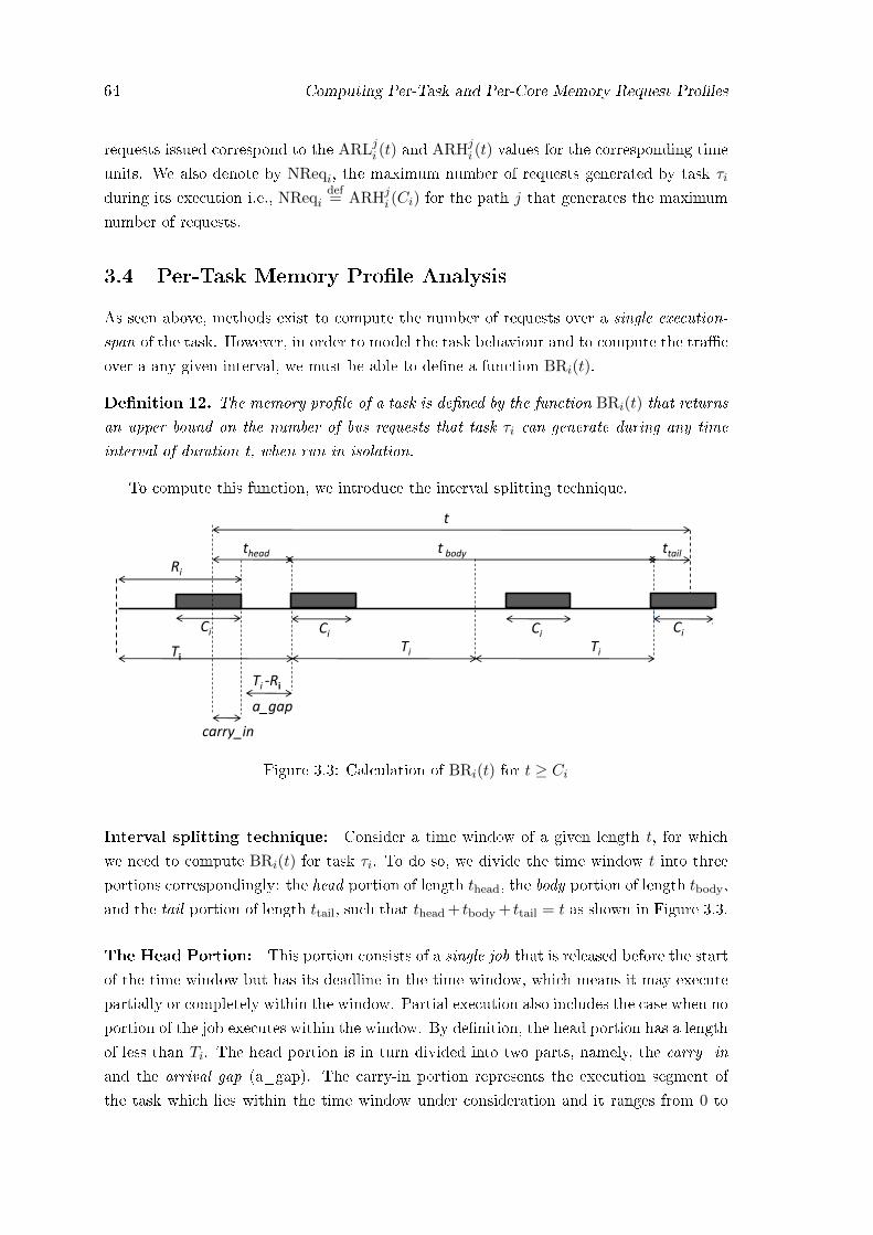
64 Computing Per-Task and Per-Core Memory Request Pro�les
requests issued correspond to the ARLji (t) and ARHji (t) values for the corresponding time
units. We also denote by NReqi, the maximum number of requests generated by task τiduring its execution i.e., NReqi
def= ARHj
i (Ci) for the path j that generates the maximum
number of requests.
3.4 Per-Task Memory Pro�le Analysis
As seen above, methods exist to compute the number of requests over a single execution-
span of the task. However, in order to model the task behaviour and to compute the tra�c
over a any given interval, we must be able to de�ne a function BRi(t).
De�nition 12. The memory pro�le of a task is de�ned by the function BRi(t) that returns
an upper bound on the number of bus requests that task τi can generate during any time
interval of duration t, when run in isolation.
To compute this function, we introduce the interval splitting technique.
t
Ti
Ci Ci Ci Ci Ti Ti
thead t body ttail
Ri
carry_in
Ti -Ri
a_gap
Figure 3.3: Calculation of BRi(t) for t ≥ Ci
Interval splitting technique: Consider a time window of a given length t, for which
we need to compute BRi(t) for task τi. To do so, we divide the time window t into three
portions correspondingly: the head portion of length thead, the body portion of length tbody,
and the tail portion of length ttail, such that thead + tbody + ttail = t as shown in Figure 3.3.
The Head Portion: This portion consists of a single job that is released before the start
of the time window but has its deadline in the time window, which means it may execute
partially or completely within the window. Partial execution also includes the case when no
portion of the job executes within the window. By de�nition, the head portion has a length
of less than Ti. The head portion is in turn divided into two parts, namely, the carry_in
and the arrival gap (a_gap). The carry-in portion represents the execution segment of
the task which lies within the time window under consideration and it ranges from 0 to

3.4 Per-Task Memory Pro�le Analysis 65
Ci. On the other hand, the a_gap part represents the time between the completion of one
job of τi and its next release and as shown in the �gure has a length of Ti −Ri, where Rias described earlier, is the response time of the job, and represents the time between the
arrival of the job and its completion.
To summarize,
theaddef=
carry_in + a_gap if carry_in > 0
0 otherwise
with 0 ≤ carry_in ≤ Ci and a_gap = Ti −Ri
The Body Portion: This portion consists of job(s) that are released within this time
window and complete their entire execution within it. For a task τi, with minimum in-
terarrival time Ti, the length of the body portion is given by can range from 0 ≤ tbody ≤⌊tTi
⌋× Ti.
The Tail Portion: This portion consists of a single job released within the given
time window but has its deadline outside the window and hence may execute partially or
completely within the time window. By de�nition, the tail portion has a length of less
than Ti or 0 ≤ ttail ≤ Ti.
Having given an overview of the interval splitting technique, we next formulate a
method (see Algorithm 1) which computes the maximum number of requests in an in-
terval of time t, using the aforementioned concepts.
3.4.1 Algorithm to compute BRi(t)
Algorithm 1 describes a method to compute the function BRi(t). The input to the algo-
rithm is t, the duration for which the number of requests needs to be upper bounded, Ri,
the response time of the task, Ci and Ti. When the task is run in isolation, we trivially set
Ri = Ci. The algorithm computes the maximum number of requests by considering every
feasible combination of thead, tbody and ttail.
Setting the length of each portion: The algorithm proceeds by initially �xing the
carry_in part of the head portion which ranges from 0 to Ci and computes the arrival
gap given by Ti − Ri. It then correspondingly calculates tbody portion as described in
Equation 3.1. Finally the tail portion is assigned to the remaining portion of the time
interval, as described in Equation 3.2. The assignment is also re�ected in lines 3 to 16 of

66 Computing Per-Task and Per-Core Memory Request Pro�les
Algorithm 1: ComputeBR()input : Ri, Ci, Ti and time interval toutput: BRi(t)
1 begin2 total← maxreq← 0 ;3 for carry_in← 0 to min(Ci, t) do4 if (carry_in == 0) then5 thead ← 0 ;
6 tbody ←⌊tTi
⌋× Ti;
7 ttail ← t− tbody;8 else9 a_gap← Ti −Ri;
10 thead ← carry_in + a_gap;11 if thead > t then tbody ← ttail ← 0 ;12 else
13 tbody ←⌊t−theadTi
⌋× Ti;
14 ttail ← t− thead − tbody;15 end
16 end17 total← fHi (carry_in) + fMi (tbody) + fTi (ttail);18 if total > maxreq then maxreq← total
19 end20 if t < Ci then21 Compute maxreq1 as per Equation (3.6) ;22 if maxreq1 > maxreq then maxreq← maxreq1
23 end24 return maxreq ;25 end
the algorithm.
tbodydef= max
{0,
⌊(t− thead)
Ti
⌋}× Ti (3.1)
ttaildef= max {0, t− thead − tbody} (3.2)
Once the lengths of these portions are decided, the maximum number of requests that can
be generated by the task in the corresponding portions is determined.
Computing the number of requests in each portion: The head portion: As said
earlier, the head portion of τi consists of two parts: the carry_in and the a_gap. Since the
task executes in the carry-in portion, it represents the portion of the head segment where
requests are issued. On the other hand, the a_gap part represents the time between the
completion of one job of τi and its next release; and therefore in the a_gap portion of the

3.4 Per-Task Memory Pro�le Analysis 67
head, no bus requests can be generated. An upper bound on the number of bus requests
generated in the head portion is given therefore by:
fheadi (thead)
def= fhead
i (carry_in)def= max
j∈paths(τi)
{ARHj
i (Cji )−ARLji ([C
ji − carry_in])
}(3.3)
The body portion: In the body portion, there are exactly tbody/Ti complete executions of
τi and the maximum number of request generated in the body portion is given by:
fbodyi (tbody)
def=
tbody
Ti× maxj∈paths(τi)
{ARHj
i (Cji )}
(3.4)
The tail portion: Finally, the length of the tail part is less than Ti, implying either one
partial or one complete execution. The number of bus requests generated in the tail part
can be bounded from above by:
f taili (ttail)
def= max
j∈paths(τi)
{ARHj
i (min{ttail, Cji })}
(3.5)
For every combination of thead, tbody and ttail, the algorithm computes the number of
requests in line 17. The maximum recorded value of the number of requests generated is
updated as the algorithm proceeds and the �nal value is returned as BRi(t).
t
Ci
time
s+t s
Figure 3.4: Calculation of BRi(t) for t < Ci
For the special case in which t < Ci (Line 20), the maximum number of requests may
be generated across two jobs (with only a carry_in and tail portion, and no body portion),
or in any arbitrary segment of the task. In the latter case, we compute BRi(t) as per
Equation 3.6, illustrated in Figure 3.4.
BRi(t) = maxj∈paths(τi)
0≤s<(Ci−t)
{ARHj
i (min{s+ t, Cji })−ARLji (s)}
(3.6)
3.4.2 Illustration of Computation of BRi(t)
To illustrate the computation of the BRi(t) function, given the values of ARHji (t), ARLji (t),
we consider a request pattern for task τi with a single execution path. We therefore drop
the path index for readability in this example. The analyzed task τi has a Ci of 5 time
units and Ti of 10 time units. The number of requests presented in Table 3.1 show the
ARHi(t) and ARLi(t) values for the task during its execution i.e., ∀t ∈ [1 . . . 5]. For this
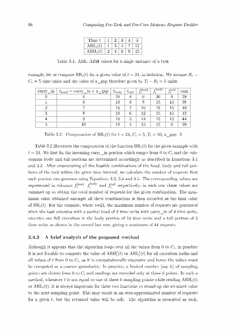
68 Computing Per-Task and Per-Core Memory Request Pro�les
Time t 1 2 3 4 5ARLi(t) 1 3 5 7 12ARHi(t) 2 4 6 9 15
Table 3.1: ARL, ARH values for a single instance of a task
example, let us compute BRi(t) for a given value of t = 24, in isolation. We assume Ri =
Ci = 5 time units and the value of a_gap therefore given by Ti −Ri = 5 units.
carry_in thead = carry_in + a_gap tbody ttail fheadi fbody
i f taili sum
0 0 20 4 0 30 9 391 6 10 8 8 15 15 382 7 10 7 10 15 15 403 8 10 6 12 15 15 424 9 10 5 14 15 15 44
5 10 10 4 15 15 9 39
Table 3.2: Computation of BRi(t) for t = 24, Ci = 5, Ti = 10, a_gap=5
Table 3.2 illustrates the computation of the function BRi(t) for the given example with
t = 24. We �rst �x the incoming carry_in portion which ranges from 0 to Ci and the sub-
sequent body and tail portions are determined accordingly as described in Equations 3.1
and 3.2. After enumerating all the feasible combinations of the head, body and tail por-
tions of the task within the given time interval, we calculate the number of requests that
each portion can generate using Equations 3.3, 3.4 and 3.5. The corresponding values are
represented in columns fheadi , fbody
i and f taili respectively; in each row these values are
summed up to obtain the total number of requests for the given combination. The max-
imum value obtained amongst all these combinations is then recorded as the �nal value
of BRi(t). For the example, where t=24, the maximum number of requests are generated
when the task executes with a partial head of 9 time units with carry_in of 4 time units,
executes one full execution in the body portion of 10 time units and a tail portion of 5
time units, as shown in the second last row, giving a maximum of 44 requests.
3.4.3 A brief analysis of the proposed method
Although it appears that the algorithm loops over all the values from 0 to Ci, in practice
it is not feasible to compute the value of ARHji (t) or ARLji (t) for all execution paths and
all values of t from 0 to Ci, as it is computationally expensive and hence the values must
be computed at a coarser granularity. In practice, a limited number (say k) of sampling
points are chosen from 0 to Ci and readings are recorded only at these k points. In such a
method, whenever t is not equal to one of these k sampling points while reading ARHi(t)
or ARLi(t), it is always important for these two functions to round-up the returned value
to the next sampling point. This may result in an over-approximated number of requests
for a given t, but the returned value will be safe. The algorithm is presented as such,
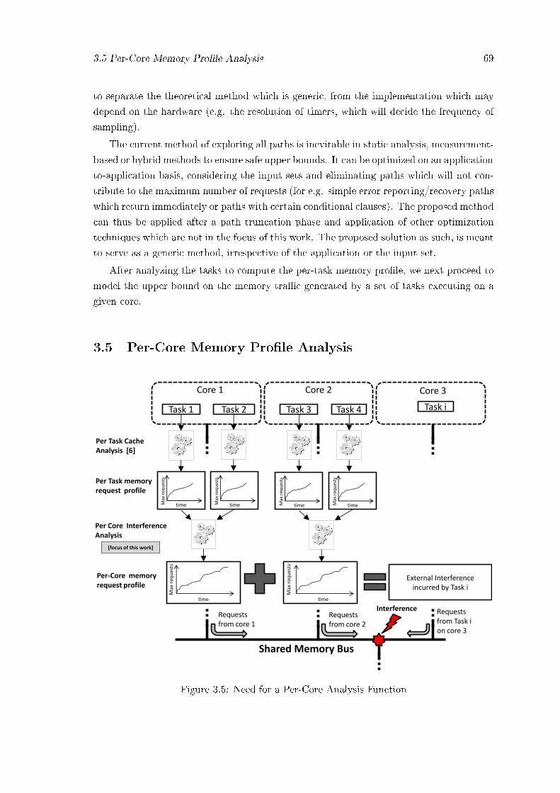
3.5 Per-Core Memory Pro�le Analysis 69
to separate the theoretical method which is generic, from the implementation which may
depend on the hardware (e.g. the resolution of timers, which will decide the frequency of
sampling).
The current method of exploring all paths is inevitable in static analysis, measurement-
based or hybrid methods to ensure safe upper bounds. It can be optimized on an application-
to-application basis, considering the input sets and eliminating paths which will not con-
tribute to the maximum number of requests (for e.g. simple error reporting/recovery paths
which return immediately or paths with certain conditional clauses). The proposed method
can thus be applied after a path truncation phase and application of other optimization
techniques which are not in the focus of this work. The proposed solution as such, is meant
to serve as a generic method, irrespective of the application or the input set.
After analyzing the tasks to compute the per-task memory pro�le, we next proceed to
model the upper bound on the memory tra�c generated by a set of tasks executing on a
given core.
3.5 Per-Core Memory Pro�le Analysis
Task 1 Task 2 Task 3 Task 4
External Interference incurred by Task i
Core 1
Per Task Cache Analysis [6]
Per Task memory request profile
Per Core Interference Analysis
Per-Core memory request profile
time
Max
req
ues
ts
time
Max
req
ues
ts
[focus of this work]
time Max
req
ues
ts
time Max
req
ues
ts
Core 2 Core 3
Task i
Shared Memory Bus
Requests from core 1
Requests from core 2
Requests from Task i on core 3
time Max
req
ues
ts
time Max
req
ues
ts
Interference
Figure 3.5: Need for a Per-Core Analysis Function

70 Computing Per-Task and Per-Core Memory Request Pro�les
De�nition 13. The Per-Core Memory Pro�le of a task represents the maximum number
of requests that can be generated by the set of tasks assigned to a given core πp, in any time
interval of length t and is given by the function PCRPp(t), short for Per-Core-Request-
Pro�ler.
This section describes the role of this function and proposes a method to compute it.
3.5.1 Role of the PCRP functions in the analysis cycle
Suppose that we have to compute the WCET of a task τi when it runs in conjunction with
other tasks in a multicore system. As depicted in Figure 3.5 (which is repeated here to
ease readability), let us consider a system with 4 cores (with core 4 being idle; hence not
shown in the diagram). Tasks τ1 and τ2 are assigned to core π1, and tasks τ3 and τ4 are
assigned to core π2. The analyzed task τi is assigned to Core 3.
To compute the WCET of task τi considering the contention on the shared bus, it is
necessary to estimate the maximum interference (in terms of memory requests) that τican incur during its execution. In this example, the interference can be attributed to the
requests issued from tasks co-executing on cores 1 and 2. For each of these two cores, it
is thus necessary to derive a function that computes an upper-bound on the number of
requests that the cores may issue during the execution of τi, because every request issued by
cores 1 and 2 may potentially compete for the bus with a request of τi, and thus contribute
to the total interference incurred by τi.
A prerequisite to derive these two required functions PCRP1() and PCRP2() is the
memory request pro�le of each task, assigned to these 2 cores. For a given task, the
maximum number of requests that it can generate in a given time window can be obtained
by the interval splitting technique described in the previous section. For each core π1 and
π2, the individual memory pro�le of each task assigned to it, along with other parameters
like the task minimum inter-arrival times and their WCET in isolation are then fed into
an analysis framework to derive the per-core memory pro�le i.e., the functions PCRP1()
and PCRP2(). The computed per-core memory pro�les can be used to derive the total
interference posed by cores π1 and π2 to the analyzed task τi assigned to core π3.
It must be noted that pessimistic estimates of the WCETs can lead to over-dimensioning
the system resources. The WCET is a key input to the schedulability analysis; this analysis
is carried out at design time to ensure that all tasks in the system will meet their deadlines
during run-time. In the absence of tight WCET estimates, many tasks may be (wrongly)
deemed unschedulable. The function PCRPp(t) is thus a vital intermediate tool in the
analysis cycle. The main focus of this section is compute such a function and show how it
can be seamlessly integrated in the higher level analysis.

3.5 Per-Core Memory Pro�le Analysis 71
3.5.2 An basic additive method to compute the PCRP functions
In the previous section we studied a method to model the memory pro�le of a task by the
BRj(t) function which returns an upper bound on the number of bus requests that task τjcan generate in time t. Let τp represent the set of tasks assigned to core πp. Then a basic
method to compute the total interference from all the tasks running on core πp is inferred
simply by adding up the functions BRj(t) of all the tasks τj assigned to that core πp, as
described in the following equation.
PCRPp(t) =∑∀τj∈πp
BRj(t) (3.7)
Before we present a better solution, we understand the role of PCRP() and the demerits
of this particular approach by applying it to determine the response time of a task.
3.5.2.1 General Response-Time Analysis
The research literature provides methods for computing the worst-case response-time of
tasks scheduled by non-preemptive �xed-priority scheduling on uniprocessor system [92,
93]. For the task model considered in this paper, an equation for the response time can be
derived from [95] by applying the following recursive equation:
R̂(k+1)i = Ci +Bi +
∑j∈hp(i)
⌈R̂kiTj
⌉× Cj (3.8)
where Bi is the maximum blocking time imposed on task τi due to lower-priority tasks, i.e.,
Bidef= maxj∈lp(i){Cj}. The WCRT Ri of the task τi is computed in an iterative manner,
starting from R̂(0)i = Ci + Bi, and is given by the smallest value of R̂ki that satis�es
Equation (3.8). The process terminates when either it reaches the �rst �xed-point value of
the equation at which R̂(k+1)i = R̂
(k)i , in which case the WCRT Ri is given by the value of
R̂(k+1)i . Alternatively the computation terminates when R̂(k+1)
i > Di with the implication
that the deadline of task τi is missed.
3.5.2.2 Extended Response-Time analysis
The computation of the WCRT in the multicore scenario must consider the increased delay
due to tasks executing on the same core and the additional delays due to contention on the
FSB from tasks running on the other cores. We now introduce the extended response-time
equation which, in addition to the original WCRT equation, also factors-in the contention
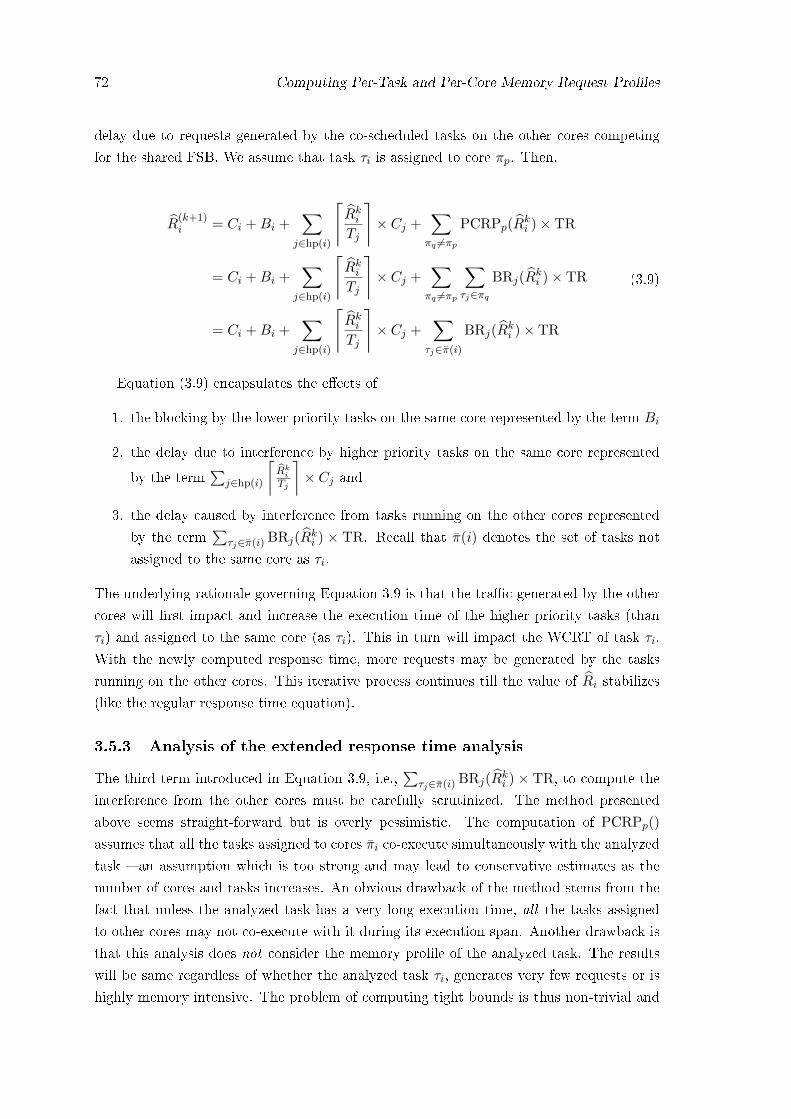
72 Computing Per-Task and Per-Core Memory Request Pro�les
delay due to requests generated by the co-scheduled tasks on the other cores competing
for the shared FSB. We assume that task τi is assigned to core πp. Then,
R̂(k+1)i = Ci +Bi +
∑j∈hp(i)
⌈R̂kiTj
⌉× Cj +
∑πq 6=πp
PCRPp(R̂ki )× TR
= Ci +Bi +∑
j∈hp(i)
⌈R̂kiTj
⌉× Cj +
∑πq 6=πp
∑τj∈πq
BRj(R̂ki )× TR
= Ci +Bi +∑
j∈hp(i)
⌈R̂kiTj
⌉× Cj +
∑τj∈π̄(i)
BRj(R̂ki )× TR
(3.9)
Equation (3.9) encapsulates the e�ects of
1. the blocking by the lower priority tasks on the same core represented by the term Bi
2. the delay due to interference by higher priority tasks on the same core represented
by the term∑
j∈hp(i)
⌈R̂kiTj
⌉× Cj and
3. the delay caused by interference from tasks running on the other cores represented
by the term∑
τj∈π̄(i) BRj(R̂ki ) × TR. Recall that π̄(i) denotes the set of tasks not
assigned to the same core as τi.
The underlying rationale governing Equation 3.9 is that the tra�c generated by the other
cores will �rst impact and increase the execution time of the higher priority tasks (than
τi) and assigned to the same core (as τi). This in turn will impact the WCRT of task τi.
With the newly computed response time, more requests may be generated by the tasks
running on the other cores. This iterative process continues till the value of R̂i stabilizes
(like the regular response time equation).
3.5.3 Analysis of the extended response time analysis
The third term introduced in Equation 3.9, i.e.,∑
τj∈π̄(i) BRj(R̂ki ) × TR, to compute the
interference from the other cores must be carefully scrutinized. The method presented
above seems straight-forward but is overly pessimistic. The computation of PCRPp()
assumes that all the tasks assigned to cores π̄i co-execute simultaneously with the analyzed
task � an assumption which is too strong and may lead to conservative estimates as the
number of cores and tasks increases. An obvious drawback of the method stems from the
fact that unless the analyzed task has a very long execution time, all the tasks assigned
to other cores may not co-execute with it during its execution span. Another drawback is
that this analysis does not consider the memory pro�le of the analyzed task. The results
will be same regardless of whether the analyzed task τi, generates very few requests or is
highly memory intensive. The problem of computing tight bounds is thus non-trivial and
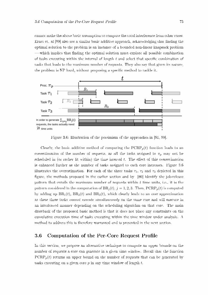
3.6 Computation of the Per-Core Request Pro�le 73
cannot make the above basic assumption to compute the total interference from other cores.
Ernst et. al [80] also use a similar basic additive approach, acknowledging that �nding the
optimal solution to the problem is an instance of a bounded non-linear knapsack problem
� which implies that �nding the optimal solution must explore all possible combination
of tasks executing within the interval of length t and select that speci�c combination of
tasks that leads to the maximum number of requests. They also say that given its nature,
the problem is NP-hard, without proposing a speci�c method to tackle it.
...
In order to generate
requests, the tasks actually need
time units
Proc.
Task
Task
Task
∑τjϵπpBRj(t)
Figure 3.6: Illustration of the pessimism of the approaches in [91, 80].
Clearly, the basic additive method of computing the PCRPp(t) function leads to an
overestimation of the number of requests, as all the tasks assigned to πp may not be
scheduled in (or rather �t within) the time interval t. The e�ect of this overestimation
is enhanced further as the number of tasks assigned to each core increases. Figure 3.6
illustrates the overestimation. For each of the three tasks τ1, τ2 and τ3 depicted in this
�gure, the methods proposed in the earlier section and by [80] identify the job-release
pattern that entails the maximum number of requests within t time units, i.e., it is the
pattern considered in the computation of BRj(t), j = 1, 2, 3. Then, PCRPp(t) is computed
by adding up BR1(t), BR2(t) and BR3(t), which clearly leads to an over-approximation
as these three tasks cannot execute simultaneously on the same core and will execute in
an interleaved manner depending on the scheduling algorithm on that core. The main
drawback of the proposed basic method is that it does not place any constraints on the
cumulative execution time of tasks executing within the time window under analysis. A
method to address this is therefore warranted and is presented in the next section.
3.6 Computation of the Per-Core Request Pro�le
In this section, we propose an alternative technique to compute an upper bounds on the
number of requests a core can generate in a given time window. Recall that the function
PCRPp(t) returns an upper bound on the number of requests that can be generated by
tasks executing on a given core p in any time window of length t.
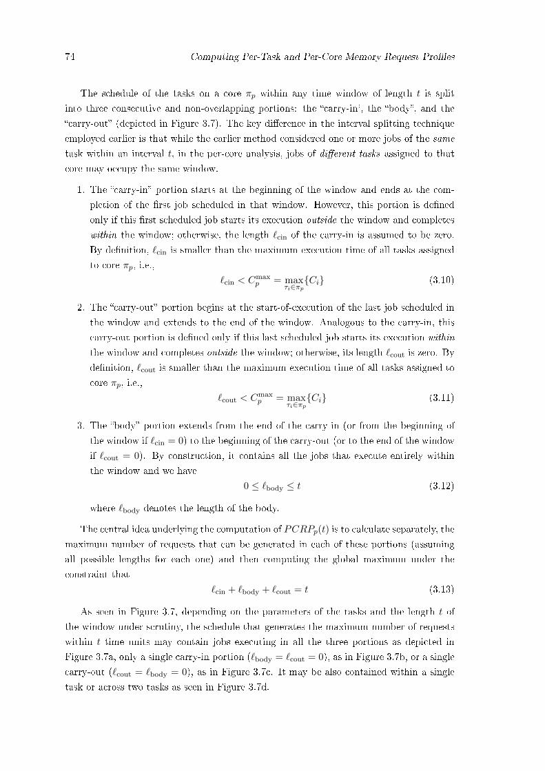
74 Computing Per-Task and Per-Core Memory Request Pro�les
The schedule of the tasks on a core πp within any time window of length t is split
into three consecutive and non-overlapping portions: the �carry-in', the �body�, and the
�carry-out� (depicted in Figure 3.7). The key di�erence in the interval splitting technique
employed earlier is that while the earlier method considered one or more jobs of the same
task within an interval t, in the per-core analysis, jobs of di�erent tasks assigned to that
core may occupy the same window.
1. The �carry-in� portion starts at the beginning of the window and ends at the com-
pletion of the �rst job scheduled in that window. However, this portion is de�ned
only if this �rst scheduled job starts its execution outside the window and completes
within the window; otherwise, the length `cin of the carry-in is assumed to be zero.
By de�nition, `cin is smaller than the maximum execution time of all tasks assigned
to core πp, i.e.,
`cin < Cmaxp = max
τi∈πp{Ci} (3.10)
2. The �carry-out� portion begins at the start-of-execution of the last job scheduled in
the window and extends to the end of the window. Analogous to the carry-in, this
carry-out portion is de�ned only if this last scheduled job starts its execution within
the window and completes outside the window; otherwise, its length `cout is zero. By
de�nition, `cout is smaller than the maximum execution time of all tasks assigned to
core πp, i.e.,
`cout < Cmaxp = max
τi∈πp{Ci} (3.11)
3. The �body� portion extends from the end of the carry-in (or from the beginning of
the window if `cin = 0) to the beginning of the carry-out (or to the end of the window
if `cout = 0). By construction, it contains all the jobs that execute entirely within
the window and we have
0 ≤ `body ≤ t (3.12)
where `body denotes the length of the body.
The central idea underlying the computation of PCRPp(t) is to calculate separately, the
maximum number of requests that can be generated in each of these portions (assuming
all possible lengths for each one) and then computing the global maximum under the
constraint that
`cin + `body + `cout = t (3.13)
As seen in Figure 3.7, depending on the parameters of the tasks and the length t of
the window under scrutiny, the schedule that generates the maximum number of requests
within t time units may contain jobs executing in all the three portions as depicted in
Figure 3.7a, only a single carry-in portion (`body = `cout = 0), as in Figure 3.7b, or a single
carry-out (`cout = `body = 0), as in Figure 3.7c. It may be also contained within a single
task or across two tasks as seen in Figure 3.7d.

3.6 Computation of the Per-Core Request Pro�le 75
carry-in carry-out body
(a) Three portion split
carry-in
(b) Window contains theend portion of the taskonly
carry-out
(c) Window contains thebeginning portion of thetask only
(d) Window contained with a task OR Window contained across2 tasks
Figure 3.7: Illustration of interval splitting
The following subsections describe the methods of computing an upper bound on the
number of request in the carry-in, carry-out, and the body portions and the technique to
deal with the special case. We shall use the following notations: the functions inreqp(k),
outreqp(k) and breqp(k) will record the upper bounds on the number of requests generated
within k ≤ t time units on core πp in the three portions, respectively.
3.6.1 Maximization of the number of requests in the carry-in and carry-
out portions
As stated by Inequalities 3.10 and 3.11, the length of the carry-in and carry-out portions
can range from 0 to Cmaxp , the maximum of the Ci's of all the tasks assigned to core
πp. However, since the size t of the window under analysis may be less than Cmaxp , our
method computes the values of inreqp(k) and outreqp(k) for all values of k in the range 0
to min(t, Cmaxp ) as:
∀k ∈ [0,min(t, Cmaxp )] : inreqp(k)← max
τi∈πp{headi(k)} (3.14)
outreqp(k)← maxτi∈πp{taili(k)} (3.15)
The method headi(k) computes an upper bound on the number of requests that τi can
generate in the last k time units of its execution. Analogously, taili(k) is an upper bound
on the number of requests that τi can generate in the �rst k time units of its execution.

76 Computing Per-Task and Per-Core Memory Request Pro�les
3.6.2 Maximization of the number of requests in the body portion
As stated by Inequality 3.12, given a time window of size t the length of the body portion
can vary from 0 to t. Hence, the value of breqp(k) is computed for all k ∈ [0, t] by calling
the TaskPack(k) function that we outline in Algorithm 2. A description of this algorithm
follows.
∀k ∈ [0, t] : breqp(k)← TaskPack(p, k) (3.16)
Recall that NReqi denotes the maximum number of requests generated by task τi during its
complete execution span. The algorithm �TaskPack(p, k)� converts the problem of deriving
an upper-bound on the number of requests that can be issued from a core πp in a given time
interval of length k, into an instance of a 0/1 knapsack problem formulated as follows [96]:
The 0/1 knapsack problem: Given a set of items, each with a corresponding weight
and value, and a knapsack of capacity k, determine the items to be included in the knapsack
so that the cumulative weight of the items in the knapsack is less than or equal to its
maximum capacity k and the cumulative value is maximized.
The transformation of computing breqp(k) into an instance of the 0/1 knapsack problem
is carried out as follows. As stated earlier, the body portion contains only entire executions
of jobs from di�erent tasks (and/or possibly from the same task). Moreover, irrespective
of the scheduling algorithm employed, each task τi can release at most dk/Tie jobs within atime window of length k. Thus, there are
∑τi∈πp dk/Tie jobs (i.e., items) on core πp; each
job from task τi has a weight of Ci and a value of NReqi and the objective is to determine
which of these jobs (or items) to include in the time window (the knapsack) such that the
total value is maximized, but subject to the constraint that the total weight is no greater
than the given capacity k. In short, the problem is to pack the window of length t with
the set of∑
τi∈πp dk/Tie jobs such that the number of requests is maximized.
Algorithm Description The algorithm �rst transforms the problem into an instance
of a 0/1 knapsack problem [96] by creating ni = dk/Tie items 〈Ci,NReqi〉 from each task
τi ( line 7). To maximize the number of requests, a natural candidate for selection is
a job with the highest request density, i.e., the highest ratio NReqi /Ci. Therefore, the
algorithm �lls the analogous knapsack of capacity `body by traversing the list of jobs (in
descending order of NReqi /Ci) and starts packing the knapsack by �lling in upto ni items
from each τi; each (included) job of τi consumes Ci units of the knapsack while contributing
a weight of NReqi. This is essentially a greedy approach: the algorithm packs jobs within
the body window until the capacity of the knapsack (i.e., the size of the body window)
is not exceeded (lines 9-15). Note that, since this method primarily aims at computing
the maximum number of requests, and not at generating the exact schedule leading to
it, placing tasks in the order τa,τb,τa leads to the same number of requests as in the
schedule τa,τa,τb. As the items are packed, the algorithm accordingly updates the variable

3.6 Computation of the Per-Core Request Pro�le 77
Algorithm 2: TaskPack(p, `body)input : p: core index, `body: length of the body portionoutput: maxrequests
1 if (`body ≤ 0) then return 0 ;2 maxrequests← 0 ;3 foreach τi ∈ πp do4 ni ← d`body/Tie;5 end6 capacity← `body ;7 list← list containing ni items 〈Ci,NReqi〉 for each task τi ∈ πp, sorted bynon-increasing order of NReqi /Ci ;
8 rem_cap← capacity ;// Add requests of the complete tasks
9 while list 6= φ and rem_cap > 0 do10 if rem_cap− list. first().Ci ≥ 0 then11 maxrequests← maxrequests + list.first().NReqi;12 rem_cap = rem_cap− list. first().Ci;13 else14 break ;15 end16 list.deletefirst();17 end
// Add the fractional number of requests of the next task in the list
18 if list 6= φ and rem_cap > 0 then19 maxrequests← maxrequests +
rem_caplist. first().Ci
× list.first().NReqi;
20 end21 return maxrequests ;
�maxrequests� (in line 11), which holds the maximum number of requests and the variable
�rem_cap� (in line 12) which holds the currently unoccupied capacity of the knapsack.
When the last popped job cannot �t entirely in the remaining capacity, then the al-
gorithm allows a fraction of this job to �t in the remaining capacity and updates the
�maxrequests� variable by adding the corresponding number of requests, assuming that
the requests are uniformly generated over the job's execution (re�ected in line 19). This
fractional assignment transforms the problem into an instance of a fractional knapsack
problem; it is a source of pessimism in our approach but it ensures safe upper bounds on
the number of requests (as proven in the next section). It also violates our description of
the body portion in which only complete executions are permitted and can lead to a �nal
schedule containing two partial executions of jobs (one at the end of the body portion and
one in the carry-out), but given that the objective is not to draw up the optimal sched-
ule (which requires the knowledge of the scheduling algorithm), we believe that this is an
acceptable solution.
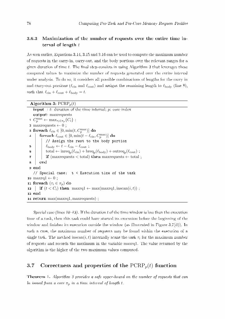
78 Computing Per-Task and Per-Core Memory Request Pro�les
3.6.3 Maximization of the number of requests over the entire time in-
terval of length t
As seen earlier, Equations 3.14, 3.15 and 3.16 can be used to compute the maximum number
of requests in the carry-in, carry-out, and the body portions over the relevant ranges for a
given duration of time t. The �nal step consists in using Algorithm 3 that leverages these
computed values to maximize the number of requests generated over the entire interval
under analysis. To do so, it considers all possible combinations of lengths for the carry-in
and carry-out portions (`cin and `cout) and assigns the remaining length to `body (line 8),
such that `cin + `cout + `body = t.
Algorithm 3: PCRPp(t)
input : t: duration of the time interval; p: core indexoutput: maxrequests
1 Cmaxp ← maxτi∈πp{Ci} ;
2 maxrequests← 0 ;3 foreach `cin ∈ [0,min(t, Cmax
p )] do
4 foreach `cout ∈ [0,min(t− `cin, Cmaxp )] do
// Assign the rest to the body portion
5 `body ← t− `cin − `cout ;6 total← inreqp(`cin) + breqp(`body) + outreqp(`cout) ;7 if (maxrequests < total) then maxrequests← total ;8 end
9 end// Special case: t < Execution time of the task
10 maxrq1← 0 ;11 foreach (τi ∈ πp) do12 if (t < Ci) then maxrq1← max(maxrq1, inscan(i, t)) ;13 end14 return max(maxrq1,maxrequests) ;
Special case (lines 10�13). If the duration t of the time window is less than the execution
time of a task, then this task could have started its execution before the beginning of the
window and �nishes its execution outside the window (as illustrated in Figure 3.7(d)). In
such a case, the maximum number of requests may be found within the execution of a
single task. The method inscan(i, t) internally scans the task τi for the maximum number
of requests and records the maximum in the variable maxrq1. The value returned by the
algorithm is the higher of the two maximum values computed.
3.7 Correctness and properties of the PCRPp(t) function
Theorem 1. Algorithm 3 provides a safe upper-bound on the number of requests that can
be issued from a core πp in a time interval of length t.
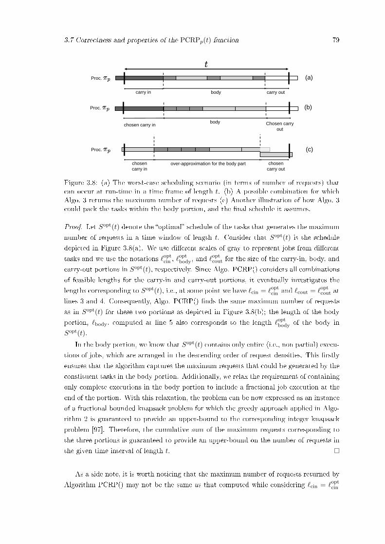
3.7 Correctness and properties of the PCRPp(t) function 79
Proc. (c)
chosen
carry in over-approximation for the body part chosen
carry out
Proc.
carry in body carry out
(a)
Proc.
chosen carry in body Chosen carry
out
(b)
Figure 3.8: (a) The worst-case scheduling scenario (in terms of number of requests) thatcan occur at run-time in a time frame of length t. (b) A possible combination for whichAlgo. 3 returns the maximum number of requests (c) Another illustration of how Algo. 3could pack the tasks within the body portion, and the �nal schedule it assumes.
Proof. Let Sopt(t) denote the �optimal� schedule of the tasks that generates the maximum
number of requests in a time window of length t. Consider that Sopt(t) is the schedule
depicted in Figure 3.8(a). We use di�erent scales of gray to represent jobs from di�erent
tasks and we use the notations `optcin , `
optbody, and `
optcout for the size of the carry-in, body, and
carry-out portions in Sopt(t), respectively. Since Algo. PCRP() considers all combinations
of feasible lengths for the carry-in and carry-out portions, it eventually investigates the
lengths corresponding to Sopt(t), i.e., at some point we have `cin = `optcin and `cout = `opt
cout at
lines 3 and 4. Consequently, Algo. PCRP() �nds the same maximum number of requests
as in Sopt(t) for these two portions as depicted in Figure 3.8(b); the length of the body
portion, `body, computed at line 5 also corresponds to the length `optbody of the body in
Sopt(t).
In the body portion, we know that Sopt(t) contains only entire (i.e., non partial) execu-
tions of jobs, which are arranged in the descending order of request densities. This �rstly
ensures that the algorithm captures the maximum requests that could be generated by the
constituent tasks in the body portion. Additionally, we relax the requirement of containing
only complete executions in the body portion to include a fractional job execution at the
end of the portion. With this relaxation, the problem can be now expressed as an instance
of a fractional bounded knapsack problem for which the greedy approach applied in Algo-
rithm 2 is guaranteed to provide an upper-bound to the corresponding integer knapsack
problem [97]. Therefore, the cumulative sum of the maximum requests corresponding to
the three portions is guaranteed to provide an upper-bound on the number of requests in
the given time interval of length t.
As a side note, it is worth noticing that the maximum number of requests returned by
Algorithm PCRP() may not be the same as that computed while considering `cin = `optcin

80 Computing Per-Task and Per-Core Memory Request Pro�les
and `cout = `optcout. The algorithm may �nd other combinations of portion lengths leading
to infeasible schedules, which over-estimate the numbers of requests generated as opposed
to an optimal schedule (as depicted in Figure 3.8c). This is due to two main reasons:
1. Firstly, it may be infeasible for a task which constitutes the carry-in portion in
Sopt(t) to have another job in the body portion of Sopt(t), because of the constraint
imposed by its minimum inter-arrival time. However, since Algo. PCRP() divides
the problem into the sub-problems of �nding the maximum number of requests in the
carry-in, carry-out portions and the body portions which are solved independently.
As a consequence, some constraints on feasible schedules may be violated in the
algorithm. This may lead to a scenario in which a task has an extra job in the
schedule constructed by PCRP() than in the optimal schedule, Sopt(t) and therefore
computing a higher number of requests than the optimal schedule.
2. The second over-approximation is attributed to the number of requests computed
in the fractional assignment of the last packed task in the body portion, and the
assumption that its requests are assumed to be uniformly distributed over its execu-
tion.
In short, the pessimism arises from a) the over-approximation made while computing
the number of requests in the body and b) the fact that the maximum number of requests
generated in each of the three portions is computed regardless of which tasks are scheduled
in the other portions, hence allowing potentially more jobs of the same task to execute
within the t time units.
The monotonicity property It is important to assess the monotonicity of the PCRPp(t)
function in order to apply it as an intermediate building block in the computation of higher
level parameters like the worst-case execution time or the response time of a task, which
in turn are key inputs for the schedulability analysis.
Property 1 (Monotonically Increasing). Given core πp and durations t1 and t2, we have
t1 ≤ t2 ⇔ PCRPp(t1) ≤ PCRPp(t2)
Proof. Let maxrequests1 and maxrequests2 be the maximum number of requests returned
by PCRPp(t1) and PCRPp(t2) (computed as per Algo. 3), respectively. Let `cin1 and `cout
1 be
the lengths of the carry-in and carry-out portions in the solution returned by PCRPp(t1).
Since all possible lengths for the carry-in and carry-out portions are considered by Algo. 3,
the computation of PCRPp(t2) considers these lengths `cin1 and `cout
1 as well. Therefore,
two cases may arise:
1. maxrequests2 is obtained for these lengths `cin1 and `cout
1 of carry-in and carry-out,
which results in a larger body portion than during the computation of maxrequests1

3.8 Optimization and Computational Complexity 81
(i.e., t2− `cin1 − `cout
1 ≥ t1− `cin1 − `cout
1 ) and thus a greater number of requests within
the body as the set of jobs that can execute within t2 − `cin1 − `cout
1 ⊇ the set of jobs
that can execute within t1 − `cin1 − `cout
1 . Hence, maxrequests2 ≥ maxrequests1.
2. maxrequests2 is obtained for di�erent lengths of carry-in and carry-out, which means
that Algo. 3 found other lengths of carry-in and carry-out for which maxrequests2 is
even greater (hence maxrequests2 ≥ maxrequests1 holds as well).
3.8 Optimization and Computational Complexity
3.8.1 Optimization by PreComputations
In the entire analysis cycle, the PCRP() function is used as in intermediate function in
the determination of key parameters like the WCET or the worst case response time of
a task and is invoked a signi�cant amount of times (with a large range of values for the
input parameter t). An optimized implementation is therefore vital for an e�cient and
scalable algorithm. This optimization can be done by pre-computing the values of all the
required parameters in Algorithm 3 upto the possible maximum ranges. As said earlier,
given a window of length t, we need to compute an upper bound on the number of requests
that a task τi assigned to core πp. Then it will su�er external interference from the tasks
executing on other cores πq 6= πp. Hence we have to compute PCRPq() for those cores to
compute the external interference.
Pre-computation range for the carry_in and the carry_out portions: Given a window
of length t, we need to compute an upper bound on the number of requests that a tasks
assigned to core πq can generate. In the carry_in and carry_out portion, a single task
τj ∈ πq may partially execute within the window and hence the length of the carry_in or
the carry_out portion for τj has a range of [0, Cj ], as shown in Equations 3.10 and 3.11.
Since any of the tasks assigned to core πq may occupy this portion, the algorithm �rst
computes Cmaxq , the maximum of the Cj 's of all the assigned tasks (line 1). Then, for
all values from 0 to Cmaxj we precompute the values leading to the maximum number of
requests in these portions. Next, we proceeds to compute the range of the body portion.
Pre-computation range for the body portions: Since the length of the three portions
must add up to t, a natural range of the body portion is [0, t]. In order to compute the
maximum range that t can take, let us consider the broader picture. Let us assume that we
employ the function PCRP() to compute the WCET of task τi assigned to core πp. In order
to do so, we maximize the cumulative interference posed to τi from tasks co-executing on
the other cores by invoking the PCRPq(t) function (for all the interfering cores πq 6= πp).
As a result of this external interference, the execution time of τi increases by a value, say
δ. Meanwhile requests issued from other cores may still keep arriving in this increased
execution time. To account for this increase, the function PCRPq() must now be invoked

82 Computing Per-Task and Per-Core Memory Request Pro�les
Algorithm 4: PreComputeAndSort(q,τi)input : q is the core index,τi is the analyzed task with deadline Di
1 Sort tasks τj ∈ πq by descending order of NReqj/Cj ;2 Cmax
q = maxτj∈πq{Cj} ;3 foreach k ∈ [0, Cmax] do4 inreqq(k) = maxτj∈πq{tailj(k)} ;5 outreqq(k) = maxτj∈πq{headj(k)} ;6 end7 foreach k ∈ [0, Di] do8 breqq(k) = TaskPack(q, k) ;9 end
with the input parameter t+δ. In order for τi to meet its deadline, its (increased) execution
time should not exceed its deadline Di: thus t must lie between 0 and Di. To reiterate,
this upper limit is chosen in the broader context of employing PCRPp() as an intermediate
step for schedulability analysis of task τi � testing whether task τi will meet its deadline
when run in conjunction with other tasks.
Algorithm 4 summarizes the precomputation step. It pre-computes the maximum num-
ber of requests that can be generated within the three portions and records the maximum
number of requests in the globally accessible inreq, breq and outreq arrays. This function
should be invoked in the initialization phase of the analysis process prior to the invocation
of PCRPq(t). This algorithm also sorts the tasks assigned on each core on the basis of
their request densities. This is a pre-requisite for Algorithm 2 (which �nds an upper bound
on the number of requests generated in the body portion).
3.8.2 Computational Complexity
Algorithm TaskPack(p, t) has a worst-case computing complexity of O(t), because in the
worst-case scenario all the tasks have a WCET of 1. Algorithm PCRP() has a complexity
of O((Cmaxp )2). Assuming that the value of headi(k) and taili(k) is given for all tasks τi and
durations k, it can be seen that the complexity of Algorithm PreComputeAndSort(πp, τj)
is O(n log(n) + n× Cmaxp +Dj × t).
It is important to note that PCRP() is an intermediate functional tool in the computa-
tion of parameters like the WCET and is invoked a signi�cant amount of times. Therefore,
although it may seem trivial, the one time pre-computation step provided by Algorithm 4,
facilitates an e�cient design by avoiding obsolete re-computations of the values of PCRP()
for the same inputs in successive invocations, thereby decreasing the cumulative analysis
time.

3.9 Adaptations of PCRP() and Integration with existing work 83
3.9 Adaptations of PCRP() and Integration with existing
work
Algorithm 3 derives a PCRP function for each core but considers a generic model wherein
there is no speci�c scheduling algorithm and no speci�c bus arbitration mechanism (except
that the bus is work-conserving). In this section we adapt the computation of this function
to di�erent settings.
3.9.1 PCRP() for synchronous periodic tasks and �xed task-level prior-
ity schedulers.
The problem of computing the PCRP functions is inherently simpler for a system in which
tasks are periodic, non-preemptive and the scheduler enforces a �xed ordering of task
execution (�xed task-level priority). Within a �xed task-level priority scheme [98], a unique
priority is associated with each task and all jobs generated by a task have the priority
associated with that task. In the case that task τ1 has higher priority than task τ2, an
activated job of τ1 will have a higher priority over an activated job of τ2. An example of
such a scheduling algorithm is the Rate Monotonic algorithm [99]. For this category of
scheduling policies, it has been shown in [100] that the entire schedule eventually repeats
(cyclic scheduling) every H units of time, where H is the period of the schedule.
Since the pattern of task arrivals is known for such a task model, it is not necessary to
�nd the combination of tasks that leads to the maximum number of bus requests. Instead,
we �rst draw up the entire schedule of the tasks from time 0 to time H + t, by considering
that every job executes for its WCET. Note that we still make the non work-conserving
assumption here, i.e., if tasks do not execute up to their WCET, the core must be idled
up to the WCET. Since the arrival times of the tasks and their execution order is known
in this task model, this schedule can be constructed at design time. Then, this schedule is
scanned by sliding a time window of length t from time 0 to time H + t. The extra t time
units beyond the period of the schedule must be considered, as the maximum number of
bus requests may be generated across two schedule periods. As the interval is scanned,
the maximum number of requests observed so far within the sliding window of length t is
recorded and is �nally returned by the PCRPp(t) function.
3.9.2 PCRP() for �xed task-level priority schedulers and a priority-
driven bus
In the context of bus arbitration policies, one of the challenges with currently existing
COTS-based multicore systems is that the front-side bus does not recognize/respect task
priorities. This is because the bus is generally designed with the aim of enhancing the
average case performance and not tailored for real-time systems. This can lead to a case
of priority inversion in which requests from higher priority tasks are delayed by requests
84 Computing Per-Task and Per-Core Memory Request Pro�les
from lower priority tasks on the bus. Although the scheduler enforces these priorities while
allocating the processing element (CPU) to tasks, these priorities are not passed over to the
shared low-level hardware resources like the bus and the memory controllers, which have
their own scheduling policies. In an interesting work [101], the authors have designed a
priority driven bus in which external priorities assigned by the operating system are passed
over to the underlying hardware upto the memory controller by tagging the request with
its priority. We shall assume for this subsection, that the bus follows such an arbitration
mechanism. Another design for a priority driven bus arbiter is proposed in [102].
Given that the scheduler on each core employs a �xed task-level priority algorithm
and the bus arbiter follows the same policy (i.e., the requests are tagged with the priority
information of the tasks they are issued from), tighter bounds can be derived. To that
end, Algorithm 3 must be slightly adapted and an important pre-requisite to derive tighter
bounds is that we must be able to assign relative priorities globally to all the tasks in the
system.
Let us assume that the analyzed task τi has a priority λ(i). To recall, the rationale
behind the proposed algorithm in order to �nd the combination of tasks which leads to the
maximum number of requests in a given interval of time t, we divide the time into three
portions: the carry-in, the carry-out, and the body portions. For each of these portions
we determine the job(s) which maximize(s) the number of requests.
1. For the carry-in portion: Pass the priority of the task to the tail() function as an
additional parameter. Unlike the earlier case in which any task could be a part of
the carry-in portion, this priority information is used to limit the selection to only
those tasks with a priority ≥ λ(i).
2. For the carry-out portion: Pass the priority of the task to the head() function as an
additional parameter. This priority information is used to narrow down the set of
candidate tasks to only those tasks with a priority ≥ λ(i).
3. For the body portion: Here the knapsack needs to be �lled in with the set of tasks
with the highest request densities. This requires a change in the way the tasks are
sorted. To capture the set of tasks which maximize the number of requests, the task
are ordered in two steps. Note that this grouping implies that, for the analyzed task,
the relative priority ordering among the tasks with a higher priority than itself is not
relevant.
(a) Split the task set into two groups: Group 1 contains all the tasks with a higher
priority than λ(i). Group 2 contains the remaining tasks.
(b) Sort the tasks in Group 1 by decreasing order of their request densities NReqi/Ci.
The body portion is packed using only the tasks ∈ Group 1.

3.9 Adaptations of PCRP() and Integration with existing work 85
The steps above ensure that a request from the analyzed task can be blocked only by
requests from higher priority tasks. The maximization phase and the rest of the logic
remains unchanged for Algorithm 3.
3.9.3 PCRP() for systems with main memories with asymmetric read
and write latencies
In the current state-of-the-art, the characterization of the memory request pro�le of tasks
generally does not di�erentiate between read and write requests and implicitly assumes
that the time to serve a read request is same as the time needed to serve a write. That
is, it is assumed in the previously proposed analyses that each request is served in a �xed
and constant time, irrespective of its type.
While this may be an acceptable assumption for DRAM-like memories for which read
and write latencies are of same order of magnitude, it does not hold for other types of
memory like Phase Change Memory (PCM) [103, 104, 105] or Flash memories, in which
write requests have a substantially higher memory latency than a read request (about 10
times higher in PCM). For systems using such memories, the assumption of equal read
and write latencies will lead to over-estimations of the timing parameters and the problem
eventually cascades to the over-allocation of system resources at design times. Hence,
the interference contributed by a read and a write transaction must be distinctly dealt
with, considering their respective worst-case service time. While Algorithm 3 returns the
maximum number of requests that can be generated in t time units, for systems with
asymmetric read/write latencies the algorithm should be adjusted to output the maximum
number of time units during which the processor will be stalling, waiting for the requests
to be served.
In order to make this adjustment, we change each of the building blocks of the PCRP()
Algorithm. First, the individual task pro�ling done by cache analysis (a pre-requisite
to the PCRP() computation) must be modi�ed to return the number of read and write
requests in a given time window of length t (instead of simply returning the number of
requests, without distinguishing between reads and writes). Task pro�ling is generally
done by measurements or with the aid of static analysis tools. For example, in the case
of experimentally pro�ling a task, many modern processors provide exclusive events (like
l2_store_misses and l2_load_misses) which enable performance monitoring counters [94]
to keep track of the number of reads and write misses. Hence, computing the PCRP()
functions in this context is practically feasible.
Let us denote by Tread and Twrite, an upper bound on the time to complete a read and
a write transaction, respectively. Also, let nread(t) and nwrite(t) denote an upper bound on
the number of read and write requests generated in a time window of length t, respectively.
1. For the carry-in portion: The task which returns the maximum delay in the carry-in
portion must be selected. That is, Algorithm 3 must select the task for which the
86 Computing Per-Task and Per-Core Memory Request Pro�les
delay computed by nread(`cin) × Tread + nwrite(`cin) × Twrite is maximized in its last
`cin time units of execution.
2. For the carry-out portion: Analogously, Algorithm 3 must select the task for which
the delay computed by nread(`cout)× Tread + nwrite(`cout)× Twrite is maximized in its
�rst `cout time units of execution.
3. For the body portion: The knapsack must be �lled in with the set of tasks with
the highest request densities. Recall that in Algorithm 3 the request density of
each task τi is de�ned as NReqi/Ci. This quantity has to be rede�ned here as
(nread(Ci)×Tread +nwrite(Ci)×Twrite)/Ci. The algorithm then proceeds as described
in Algo. 3, by sorting the tasks in decreasing order of request density.
Although the main aim of the analysis is to design a uni�ed framework using the
PCRP() function, we showcase its applicability in computing the worst-case execution
time for a given arbitration algorithm.
3.10 PCRP case study: WCET analysis
In this analysis, we assume that the contention over the FSB is resolved based on a RR
arbitration mechanism, in which all the cores are treated equally. The order in which the
cores acquire the ownership of the bus is �xed apriori. When more than one core tries to
access the bus, ties are resolved based on the �xed-ownership ordering. Given the WCET
Ci of a task τi in isolation, here we compute the extra execution time that should be added
to Ci to take into account the delay due to contention on the FSB. As mentioned earlier,
TR denotes an upper-bound on the time to serve a memory request when a task runs in
isolation and NReqi denotes the maximum number of requests the task generates over its
execution span.
3.10.1 Basic round robin equation
Given a RR bus arbitration mechanism, an upper-bound C ′i on the WCET of each task τiconsidering bus contention is given by
C ′idef= Ci + NReqi×(m− 1)× TR (3.17)
Since the access to the shared FSB is granted using the RR protocol, each request generated
by τi can be blocked by at most 1 request issued by the tasks running on each of the other
(m− 1) cores, hence creating an extra delay of at most NReqi×(m− 1)×TR time units.
Equation (3.17) implicitly assumes that the tasks running on each of the (m − 1)
interfering cores will generate NReqi requests during the execution of task τi, which might
not be true as tasks running on these cores may generate lesser number of requests. Hence

3.10 PCRP case study: WCET analysis 87
the above equation may lead to pessimistic bounds. We tackle this over-pessimism by
providing a tighter upper-bound in the following subsection.
3.10.2 Improved Round Robin equation
Lemma 1. Considering that a task τi is executing with contention on the FSB, an upper-
bound C ′i on its execution time is given by the �rst solution (i.e., Cki = Ck−1i ) at which the
following �xed-point iteration converges:
Ckidef= Ci +
∑πp∈π̄(i)
min(NReqi,PCRPp(Ck−1i ))× TR (3.18)
with C0i
def= Ci. The �xed point iteration terminates when Cki = Ck−1
i , at which, the value
of C ′i is given by the corresponding Cki .
Proof. Equation (3.18) recursively computes a new value of Ci at each iteration k ≥ 1,
and incorporates the extra delay incurred by task τi due to the requests generated by the
tasks running on the interfering cores, i.e., the cores πp ∈ π̄(i). By de�nition, we know
that τi generates at most NReqi requests during its execution. For a RR bus arbitration
algorithm, each of the interfering cores can delay every request issued by τi by at most 1
request and hence can delay the execution of τi by at most NReqi×TR time units. Hence,
at each iteration k, Equation (3.18) considers for each core πp ∈ π̄(i) the minimum between
1. the number of requests that πp might actually generate in the (currently computed)
execution time of τi (i.e. PCRPp(Ck−1i )) and
2. the maximum number of requests that can be used by πp to block τi's execution (i.e.,
NReqi).
In the next subsection, we discuss some properties of this improved RR equation.
3.10.3 Properties of the Improved RR equation
Lemma 2. In Equation (3.18), for any iteration k ≥ 1, the value of Cki monotonically
increases, i.e Cki ≥ Ck−1i
Proof. The proof is by induction. Initially, C0i = Ci and it can be inferred from Equa-
tion (3.18) that C1i ≥ C0
i . The induction step consists in showing that, if Cki ≥ Ck−1i then
Ck+1i ≥ Cki . According to Equation (3.18), the expression Ck+1
i ≥ Cki can be rewritten as
Ci +∑
πp∈π̄(i) min(NReqi,PCRPp(Cki ))× TR
≥ Ci +∑
πp∈π̄(i) min(NReqi,PCRPp(Ck−1i ))× TR

88 Computing Per-Task and Per-Core Memory Request Pro�les
By subtracting/dividing the common terms from both sides we have:
∑πp∈π̄(i) min(NReqi,PCRPp(C
ki )) ≥∑
πp∈π̄(i) min(NReqi,PCRPp(Ck−1i )) (3.19)
Given the monotonicity of the PCRPp(t) function (∀t1 ≤ t2 : PCRPp(t1) ≤ PCRPp(t2)),
stated earlier in Property 1, for any πp we have PCRPp(Cki ) ≥ PCRPp(C
k−1i ). Therefore,
only three cases may arise:
1. NReqi ≥ PCRPp(Cki ) ≥ PCRPp(C
k−1i )
2. PCRPp(Cki ) ≥ NReqi ≥ PCRPp(C
k−1i )
3. PCRPp(Cki ) ≥ PCRPp(C
k−1i ) ≥ NReqi
and it can be easily shown for all of them that
min(NReqi,PCRPp(Cki )) ≥ min(NReqi,PCRPp(C
k−1i ))
which provides Inequality (3.19) and thereby, establishes the proof.
Lemma 3. Equation (3.18) always terminates in at most (m− 1)×NReqi iterations and
may provide a tighter upper-bound than Equation (3.17).
Proof. The proof is a direct consequence of Lemma 2. The highest value of Cki is reached
when for all the other cores, it holds that PCRPp(Cki ) ≥ NReqi. In this case, Equa-
tion (3.18) becomes Ckidef= Ci+
∑πp∈π̄(i) NReqi×TR which corresponds to Equation (3.17).
In order to maximize the number of iterations to reach this highest value of Cki , we
have to consider that at each iteration k, there exists only one core π` ∈ π̄(i) such that
min(NReqi,PCRP`(Ck−1i )) = min(NReqi,PCRP`(C
k−2i )) + 1 and for all cores πp ∈ π̄(i)
with p 6= `, it is the case that min(NReqi,PCRPp(Ck−1i )) = min(NReqi,PCRPp(C
k−2i )).
In this scenario, we get Cki = Ck−1i + 1 at each iteration k and it takes (m − 1) × NReqi
iterations to reach the highest value of Cki given above. Finally, if Equation (3.18) con-
verges to a solution Cki = Ck−1i before this extreme value, then the resulting C ′i (where
C ′i = Cki ) provides a tighter upper-bound than the C ′i computed by Equation (3.17).
3.11 System wide Analysis
In this section, we describe the process of applying the method described earlier to all the
tasks in the system. Consider an example system with 2 cores {π1, π2} and 4 tasks {τ1, τ2,
τ3, τ4}. Let tasks τ1 and τ2 be assigned to π1 and tasks τ3 and τ4 be assigned to π2. We
calculate the functions PCRP1(t) and PCRP2(t) using the method described in Section 3.5
(left box in Fig. 3.9). Tasks assigned to core π1 are subject to interferences from tasks
co-scheduled on π2 and vice versa. Therefore, we compute C ′1 and C ′2 against PCRP2(t)

3.12 Performance Comparison: Simulations 89
Compute PCRPp(t): PCRP1(t) using (C1, C2) PCRP2(t) using (C3, C4)
Compute increased Ci: C’1 using PCRP2(t) C’2 using PCRP2(t) C’3 using PCRP1(t) C’4 using PCRP1(t)
Step 1 Step 2
Figure 3.9: Our system-wide analysis is a non-cyclic process.
and C ′3 and C ′4 against PCRP1(t), using the method introduced in Section 3.10 (right box
in Fig. 3.9). At this point, it may seem that the functions PCRP1(t) and PCRP2(t) can
be re�ned using as input, the newly computed C ′1, C′2, C
′3 and C ′4. If so, the process may
re-iterate and a natural question is �when should the process stop iterating?�. We answer
this question based on the following Lemma 4.
Lemma 4. For every core p, the function PCRPp(t) monotonically decreases as the WCET
of the tasks running on core πp is in�ated due to the contention for the FSB.
Proof. The proof is a consequence of the fact that incorporating the interference from
other tasks into the WCET estimate of a given task τi does not increase the number of
requests that τi can potentially generate in any time window of any length t. That is, the
number of requests that are inherently generated by each task τj assigned to πp does not
increase as its WCET in�ates. In the computation of PCRPp(t), the impact of in�ating
the WCET of each task τi (without modifying its maximum number of requests NReqi)
is that the requests of their jobs are spaced further apart (resulting in a lower request
density). Another consequence is that potentially lesser jobs of τi can execute within the
body portion and lesser requests can potentially be generated within a given length of
carry_in and carry_out portions Hence the lemma.
As proven in Lemma 4, re-iterating the process of computing PCRPp(t) (for all cores
πp) and C ′i (for all tasks τi) alternately will decrease the value returned by the function
PCRPp(t) at each iteration, hence ultimately providing an unsafe upper-bound for the
WCETs. As a result, our analysis is a one-step process, i.e., it is not cyclic. This also
means that the given model facilitates the determination of the value of C ′i for every task
τi at design-time itself.
3.12 Performance Comparison: Simulations
In this section, we will evaluate the performance of the analysis techniques developed for
deriving the memory pro�le for a given task and for a given core against the approaches
developed by contemporary researchers.
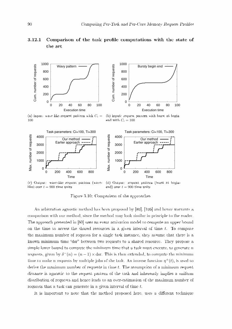
90 Computing Per-Task and Per-Core Memory Request Pro�les
3.12.1 Comparison of the task pro�le computations with the state of
the art
0
200
400
600
800
1000
0 20 40 60 80 100
Cum
. num
ber
of r
eque
sts
Execution time
Wavy pattern
(a) Input: wave-like request pattern with Ci =100
0
200
400
600
800
1000
0 20 40 60 80 100
Cum
. num
ber
of r
eque
sts
Execution time
Bursty begin end
(b) Input: request pattern with burst at begin-end with Ci = 100
0
1000
2000
3000
4000
0 200 400 600 800
Ma
x.
nu
mb
er
of
req
ue
sts
Time
Task parameters: Ci=100, Ti=300
Our methodEarlier approach
(c) Output: wave-like request pattern (wave-like) over t = 900 time units
0
1000
2000
3000
4000
0 200 400 600 800
Ma
x.
nu
mb
er
of
req
ue
sts
Time
Task parameters: Ci=100, Ti=300
Our methodEarlier approach
(d) Output: request pattern (burst at begin-end) over t = 900 time units
Figure 3.10: Comparison of the approaches
An arbitration agnostic method has been proposed by [80], [106] and hence warrants a
comparison with our method, since the method may look similar in principle to the reader.
The approach presented in [80] uses an event activation model to compute an upper bound
on the time to access the shared resources in a given interval of time t. To compute
the maximum number of requests for a single task instance, they assume that there is a
known minimum time �dsr� between two requests to a shared resource. They propose a
simple lower bound to compute the minimum time that a task must execute, to generate n
requests, given by δ−(n) = (n− 1)× dsr. This is then extended, to compute the minimum
time to make n requests by multiple jobs of the task. An inverse function η+(t), is used to
derive the maximum number of requests in time t. The assumption of a minimum request
distance is agnostic to the request pattern of the task and inherently implies a uniform
distribution of requests and hence leads to an over-estimation of the maximum number of
requests that a task can generate in a given interval of time t.
It is important to note that the method proposed here, uses a di�erent technique

3.12 Performance Comparison: Simulations 91
(compared to the method proposed in [80]) to compute the maximum number of requests
for a task in a time interval t and hence the experiments presented here are used to highlight
only that phase of the overall analysis.
The input to the analysis is a set of synthetic request patterns depicted in Figures 3.10a
and 3.10b. These patterns are representative of applications having a (i) burst of requests
at the beginning and end and (ii) wave like request distribution. In these graphs, Ci = 100,
Ti = 300 and the maximum number of requests, BR(Ci) in one task instance (referred to
Nmaxj in their approach) is 1000. The experiments are run with Ri = Ci as inputs to both
algorithms. The maximum number of requests are computed for all values of t from 0 to
900 (i.e. 3*Ti time units). Since our approach to compute BRi(t) takes into consideration,
the request pro�le of a task and is sensitive to the request pattern, the bounds computed
are tighter, as seen in Figures 3.10c and 3.10d.
As seen in the graphs, our method for determining the maximum number of requests
�rst characterizes the task behavior and then derives the bounds. In contrast, the method
proposed by Ernst et. al [80] (called the �Earlier approach� in Figures 3.10c and 3.10d), does
not consider the request distribution and base their analysis on the minimum release time
between two requests. As a result, their approach yields more pessimistic upper bounds
on the number of requests that a task can generate. We compared the two approaches
for other types of request patterns (like bursts at the beginning of the application, bursts
at the end of the application, etc.) as well and found that our method outperforms their
method. As expected, for tasks with uniform distribution of requests, both methods yield
the same upper bounds. The graphs with other patterns are not presented here due to space
limitations. Summarizing the discussion above, we believe that our approach dominates
their approach in yielding tighter upper bounds on the number of requests in a given time
interval.
3.12.2 Comparison of the per-core pro�le computations with the state
of the art
The following benchmarks from the ChStone suite [107] were used for the comparison tests.
1. ADPCM decoder: Adaptive di�erential pulse code modulation decoder
2. GSM: Linear predictive coding analysis of global system for mobile communications
3. JPEG: JPEG image decompression
4. MOTION: Motion vector decoding of the MPEG-2
5. MIPS: Simpli�ed MIPS processors
6. AES: Advanced encryption standard
7. BLOWFISH: Data encryption standard

92 Computing Per-Task and Per-Core Memory Request Pro�les
0
200
400
600
800
1000
1200
1400
0 500 1000 1500 2000 2500 3000 3500 4000 4500 5000
Upper
bound o
n r
equests
Time
Our approachEarlier approach
(a) Comparison with 3 tasks per core
0
5
10
15
20
25
30
35
40
45
0 1-10 11-20 21-30 31-40 41-50 51-60 61-70 71-100
Pe
rce
nta
ge s
amp
le p
oin
ts
Percentage Improvement Ratio
(b) PIR graph with 3 tasks per core
0
500
1000
1500
2000
2500
0 500 1000 1500 2000 2500 3000 3500 4000 4500 5000
Upper
bound o
n re
quests
Time
Our approachEarlier approach
(c) Comparison with 5 tasks per core
0
5
10
15
20
25
30
35
40
45
50
0 1-10 11-20 21-30 31-40 41-50 51-60 61-70 71-80 81-100
Pe
rce
nta
ge s
amp
le p
oin
ts
Percentage Improvement Ratio
(d) PIR graph with 5 tasks per core
0
500
1000
1500
2000
2500
3000
3500
4000
4500
5000
0 500 1000 1500 2000 2500 3000 3500 4000 4500 5000
Upper
bound o
n r
equests
Time
Our approachEarlier approach
(e) Comparison with 8 tasks per core
0
5
10
15
20
25
30
35
0 1-10 11-20 21-30 31-40 41-50 51-60 61-70 71-80 81-90 91-100
Pe
rce
nta
ge S
amp
le P
oin
ts
Percentage Improvement Ratio
(f) PIR graph with 8 tasks per core
Figure 3.11: Comparison with the approach in [91]
8. SHA: Secure hash algorithm
The tests are used to highlight that as the number of tasks assigned to a core increases,
the basic approach presented earlier in Section 3.5.2 starts producing very pessimistic
results. Recall that the basic approach considers that all tasks on the interfering cores
pose a delay to the analyzed task and adopts a basic additive approach to compute the
per-core interference, while the improved approach �nds the combination of tasks that may
�t in the time interval and also generate the maximum number of requests.
To compare the approaches, we computed an upper bound on the number of requests
generated on a given core by assuming 3 tasks, 5 tasks and 8 tasks on each core in the
above tests. It can be clearly seen in Figures 3.11a, 3.11c and 3.11e that as the number of
tasks assigned to a core increases, our improved method using the task packing algorithm
produces tighter bounds on the number of requests. The graphs also serve to illustrate the
monotonically increasing property of the PCRP() function. The graphs show the values

3.12 Performance Comparison: Simulations 93
0
100
200
300
400
500
600
700
1 2 3 4 5 6 7 8 9 10 11 12 13 14 15 16
WC
ET (
in m
illis
eco
nd
s)
Task Id
RR
Improved
Figure 3.12: WCET comparison: improved approach vs. basic RR
for PCRP() computed in the time range from 1 to 5000 units. To further quantify the
performance of the tightness, we computed the percentage distribution of improvements in
tightness for each of these three cases by deriving a metric which we term the Percentage
Improvement Ratio (PIR). At each time point t let bpcrp(t) denote the bounds computed
by the PCRP() function while bsoa denote the bounds computed by the state of the art.
Then PIR for each point is given by (bsoa() − bpcrp()) ∗ 100/(bsoa()). Hence a PIR of
25% meant that the bound computed by our approach is 25% tighter than the bounds
computed by the basic additive approach [80]. As seen in Figure 3.11b, 0.52% of the
sampled points showed no improvements, while 40+% of the sampled points showed a PIR
of 11-20 %. At the higher end less than 2% of the samples showed a PIR increase of
61-70%. Interestingly, as seen in Figure 3.11f, in the case of 5 tasks being assigned on the
core, 40+% samples showed an increase in the range 21-30% and at the higher end the
percentage of samples having a 50-60% improvement also increased. This e�ect is more
pronounced in Figure 3.11f as more samples shift towards a higher PIR. The observation is
as expected, since as more tasks are added to the system, the possibility of all of them being
co-scheduled with the analyzed task decreases and thus the pessimism of the computed
bounds of the existing additive approaches increases. A simple case with 3, 5 and 8 tasks
was enough to bring forth this drawback in the existing mechanisms.
Next we evaluate the performance of the PCRP() function for a round robin arbiter.
3.12.3 Comparison: Basic Round Robin vs Improved Round Robin
The resulting WCET of a task (when in contention for the shared resources) is sensitive to
the properties of the co-scheduled tasks (Ci, Ti, memory pro�le) besides core assignments
and the scheduling algorithm. No direct co-relation between the increase in WCET and any
individual parameter can be drawn without exhaustive tests. However, the aim here is to
validate and compare our approach and hence we provide a �proof of concept� with a small
set of tasks. We generated 16 random tasks with di�erent memory pro�les (with di�erent

94 Computing Per-Task and Per-Core Memory Request Pro�les
request densities) and assigned them to 4 di�erent cores randomly. We used Algo. 3 to
compute the PCRP() function in Eq. (3.18) to compute the WCET. As seen in Fig. 3.12,
for all the tasks, our method performs equally or better (in most cases) against the basic
RR arbitration. The tightness of the improved WCET varies from (0 to 41%). There is
no improvement using our approach for task 2 and 13, which can be explained as follows:
These tasks have a very low request density (given by NReqi /Ci) of around 2 and a low
execution time. Hence their WCET increases marginally due to the contention on the bus
and there is little scope for improvement. For tasks 1, 5, 6, 8, 16 the request densities
varied from 25 to 30 (high for this example). For such tasks, the impact of contention
is high and the tightness varied from (25-41%). The rest of the tasks showed moderate
improvements (5 to 18%) with the new approach.
While the above experiments were carried out by simulations with synthetic traces, it
was important to know if the basic parameters can be computed on a real platform. The
following section summarizes the results of the exercise.
3.13 A method to obtain the parameters experimentally
In principle, it is possible to use the substantial amount of work developed in the WCET
analysis community [10] to provide suitable bounds on ARH and ARL. However, these
approaches generally need an important amount of information about the hardware to
provide accurate results. Since it is di�cult to obtain suitably accurate documentation for
COTS hardware, those techniques might provide highly pessimistic results and we focus on
an alternative technique based on measurements, as this is still the de-facto standard in the
analysis of safety critical systems. This alternative is also preferable when the underlying
cache replacement policy is pseudo-LRU, because static/o�ine analysis methods generally
lead to highly pessimistic results for such policies (and pseudo-LRU is usually employed in
COTS-based hardware).
The approaches proposed above for task-analysis requires as an input, the parameters
TR, an upper bound on the time to complete one bus transaction. It also needs the
cache pro�le of a task modeled by the ARH and ARL values. This section details how
these values can be obtained by measurement on the actual hardware. A bus transaction
involves a sequence of sub-operations, and hence the value of TR is very hardware speci�c
and cannot be obtained from manuals provided by vendors directly, and o�ine techniques
cannot be used to compute them unless all details are provided. Thus it is necessary to
obtain them by measurement.
The experiments were carried out on an IntelTMCore2 Quad Q8300 processor consisting
of four cores placed on two dies on a single chip. Each die has two cores and each core has
its own instruction and data cache (denoted as I$ and D$). However,the two cores on the
same die share the L2 cache i.e., (i) Core-1 and Core-2 share a L2 cache on one die and
(ii) Core-3 and Core-4 share a L2 cache on another die. All the 4 cores access the main
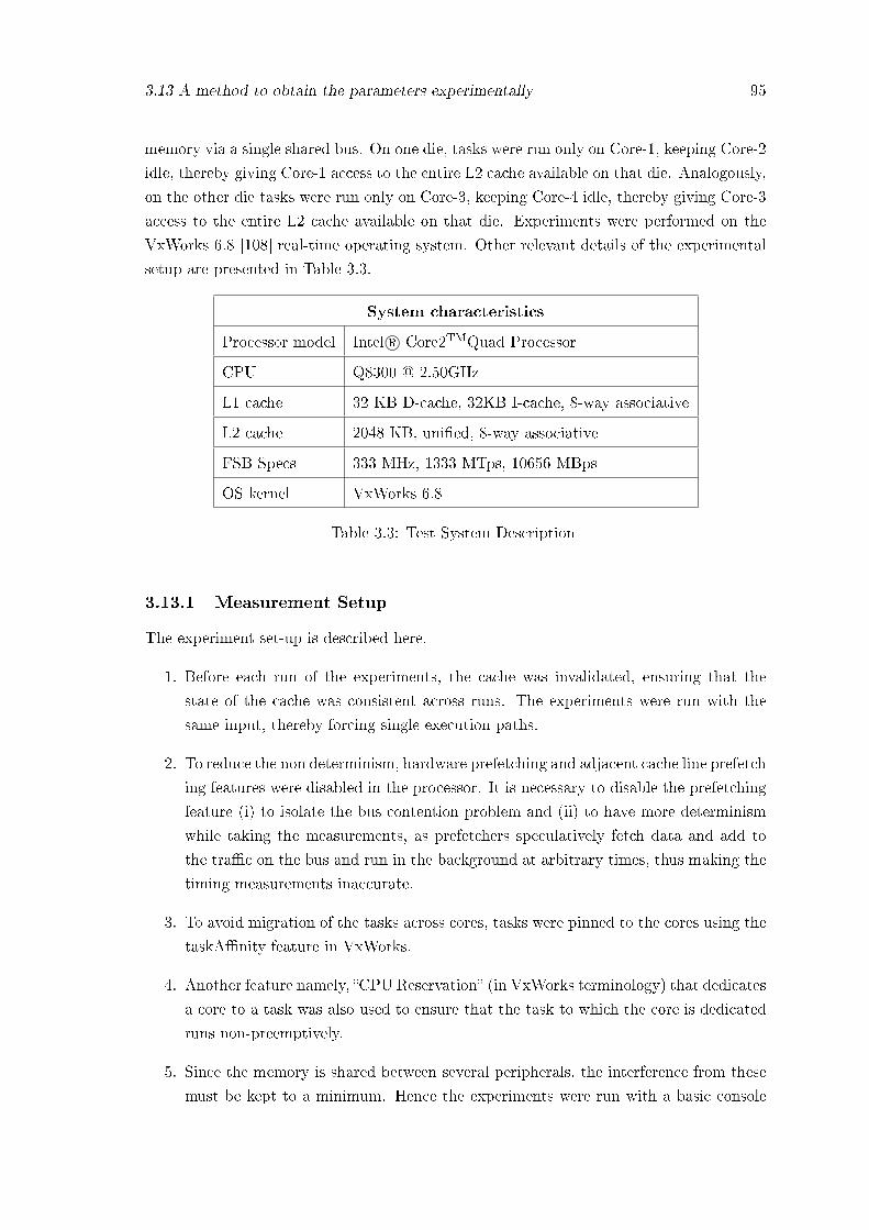
3.13 A method to obtain the parameters experimentally 95
memory via a single shared bus. On one die, tasks were run only on Core-1, keeping Core-2
idle, thereby giving Core-1 access to the entire L2 cache available on that die. Analogously,
on the other die tasks were run only on Core-3, keeping Core-4 idle, thereby giving Core-3
access to the entire L2 cache available on that die. Experiments were performed on the
VxWorks 6.8 [108] real-time operating system. Other relevant details of the experimental
setup are presented in Table 3.3.
System characteristics
Processor model Intel R© Core2TMQuad Processor
CPU Q8300 @ 2.50GHz
L1 cache 32 KB D-cache, 32KB I-cache, 8-way associative
L2 cache 2048 KB, uni�ed, 8-way associative
FSB Specs 333 MHz, 1333 MTps, 10656 MBps
OS kernel VxWorks 6.8
Table 3.3: Test System Description
3.13.1 Measurement Setup
The experiment set-up is described here.
1. Before each run of the experiments, the cache was invalidated, ensuring that the
state of the cache was consistent across runs. The experiments were run with the
same input, thereby forcing single execution paths.
2. To reduce the non determinism, hardware prefetching and adjacent cache line prefetch-
ing features were disabled in the processor. It is necessary to disable the prefetching
feature (i) to isolate the bus contention problem and (ii) to have more determinism
while taking the measurements, as prefetchers speculatively fetch data and add to
the tra�c on the bus and run in the background at arbitrary times, thus making the
timing measurements inaccurate.
3. To avoid migration of the tasks across cores, tasks were pinned to the cores using the
taskA�nity feature in VxWorks.
4. Another feature namely, �CPU Reservation� (in VxWorks terminology) that dedicates
a core to a task was also used to ensure that the task to which the core is dedicated
runs non-preemptively.
5. Since the memory is shared between several peripherals, the interference from these
must be kept to a minimum. Hence the experiments were run with a basic console
96 Computing Per-Task and Per-Core Memory Request Pro�les
device and a diskless system to avoid any DMA activity to in�uence measurement
results. the arbitration overhead and contention in the memory controller unit is
minimal in our setup.
Events were monitored at the micro-architectural level by writing to model-speci�c registers
and reading Performance Monitoring Counters (PMCs) directly. PMCs are a set of special-
purpose registers built into modern microprocessors to store the counts of hardware related
activities, such as cache misses ([94], [109]).
3.13.2 Measurement of TR
TR is de�ned as an upper bound on the time to complete one bus transaction. To obtain
this value experimentally, a task called the cache thrasher (CTC) was generated that
constantly accessed the memory and generated an L2 cache miss on each access. We
programmed this task by declaring an array twice the size of the cache and accessing each
line of the cache sequentially, thereby causing an L2 miss for every access. Since the array
size is twice the cache size, the task scans the entire cache twice in each run, hence evicting
all the cache lines that were already fetched, prior to the next run. The number of bus
requests, denoted by NBR, is obtained by monitoring the Bus_Requests_Mem event, for
each run and the time taken for each run, denoted by TBR is recorded. The number of
bus requests generated was veri�ed against the expected number of bus requests (which is
twice the number of cache lines) to validate the approach and was found to be consistent.
The value of TR is thus computed for thousands of runs and the maximum is recorded
over all the runs. Then the �nal TR is given by Equation (3.20).
TR = maxk=1..nr
(TBRk /NBRk) (3.20)
where k denotes the run index, nr denotes the number of runs and TBRk and NBRk denote
the corresponding values in that run. The value of TR from the experiments was 46.6 nano
seconds.
3.13.3 Measurement of ARH and ARL
The ARH and the ARL values described earlier, represent an upper and lower bound on the
number of bus requests generated by a task from the beginning of its execution up to time
t. To measure these values for a given task, we chose some sampling points by dividing the
execution time of the tasks into subintervals. We obtained the cumulative number of bus
requests upto that point by interrupting the task and reading the performance monitoring
counters at the required sampled point. We then re-ran the task and interrupted the
task at the next sampling point. At each sampling point, the highest measured value was
recorded as ARH and the lowest value was recorded as ARL, over multiple iterations. It is
to be noted that unlike simulations, where it is assumed that a task will have �xed number

3.14 Chapter Summary 97
Figure 3.13: ARH, ARL Curve for the Search Benchmark
of memory accesses at a given time instance, this presents a more realistic approach, as it
takes into account the variations in the number of requests issued due to the underlying
cache replacement policy employed and makes this method very generic. We also recorded
the exact time when the interrupt was issued and the time time at which the interrupt
service routine was �red to increase the precision of our results. For the given system, the
Bus_Requests_Mem_This_Core_This_Agent event was monitored to precisely measure
the number of requests issued by the task. An example of the cache analysis pro�le,
showing the ARH and ARL values at each sampling point for the Search Benchmark from
the MiBench Suite [110] is presented in Figure 3.13. The graph for the search program
shows a variability in the number of cache misses across runs during one complete execution.
It can be seen that after a certain time, the number of bus requests reaches a plateau and
then increases again. This decline in the slope to reach a plateau form, seen in the graph
corresponds to the time when the task is not issuing any requests and this was achieved
by the introduction of a task delay in the program (to demonstrate the variability in the
request pattern which can be captured by PMCs).
3.14 Chapter Summary
In this chapter, we de�ned the system and task model under which the analysis holds and
presented two primary tools, the per-task memory pro�ler and the per-core memory pro-
�ler that will be leveraged in the upcoming interference analysis aimed at determining the
WCET of a task contending with other tasks for the shared bus. The primary focus was to-
wards characterizing the memory usage pattern of a task and determining the interference
it can incur from the co-executing tasks assigned to other cores. The methods developed
employed an interval splitting technique to determine the maximum number of requests
than can be issued in a given interval of time by a given core. It was shown through simu-
lations that the proposed methods perform better than the existing approaches. Further,

98 Computing Per-Task and Per-Core Memory Request Pro�les
the properties and the computational complexity of these methods was analyzed. An appli-
cation of the Per-Core Request pro�ler was demonstrated with respect to the round robin
arbitration algorithm. It is important to note that both these methods are independent
of the bus arbitration mechanism and only deal with the amount of tra�c reaching the
shared bus from any core in a given interval of time t. The scheduling of the requests will
next depend on the arbitration mechanism of the bus and will decide the delay incurred by
each of the requests. The cumulative delay incurred by all the requests from a task along
with its execution time in isolation will eventually lead us to the �nal WCET of the task
in contention. In the next chapter, with the help of the tools developed here, an analysis
of the delay due to contention on the memory bus will be computed.

Chapter 4
Uni�ed Framework for Bus
Contention Analysis in Multicores
One ring to rule them all, one ring to �nd them,
One ring to bring them all and in the darkness
bind them.
J. R. R. Tolkien, Lord of the Rings
The previous chapter laid the foundations for the upcoming analysis � we systemati-
cally developed a per-core memory request pro�ler (or the PCRPp(t) function) to determine
the amount of memory tra�c that a core πp can inject into the front side bus in a given
interval of time t. Recall that the per-core memory request pro�ler models only the tra�c
injected into the bus, and as a result is agnostic of the underlying arbitration mechanism
employed by the bus. As a next step in the analysis, we leverage the information provided
by the per-core memory request pro�ler, together with the front side bus arbitration mod-
els, in order to achieve the objective of determining the increased execution time of the
tasks due to contention on the shared bus. The main focus of this chapter is to design a
framework that provides a common interface to di�erent arbitration algorithms and apply
this framework to compute an upper bound on the execution time of tasks when run in
conjunction with other co-executing tasks.
The need for a uni�ed framework stems from the fact that existing works address the
problem of deriving an upper bound on the delay due to bus contention to some extent,
but the analysis is tightly coupled to a particular arbitration policy, such as TDM [90,
73, 74, 75, 76] or non-speci�ed work-conserving arbiters [91, 80], and do not provide a
common mechanism to handle di�erent arbitration mechanisms. As a result, worst-case
execution time estimation tools are limited to di�erent point solutions for each system
under analysis, complicating implementation and maintenance. We address this problem
by proposing a general framework for shared bus contention analysis that addresses a wide
99

100 Uni�ed Framework for Bus Contention Analysis in Multicores
range of arbitration policies in multi-core systems and can be implemented in worst-case
execution time estimation tools.
The next section introduces the system model used in this chapter. First, we present the
platform model, followed by a characterization of tasks and their corresponding memory
pro�les. We then explain the assumptions on the task scheduler, before arriving at the
problem statement.
4.1 System and Task Modeling
We revisit the notations in this chapter to avoid re-referencing backwards in the documents.
4.1.1 Platform Model
The assumed multicore platform π contains m cores denoted by π1, π2, . . . , πm. It is as-
sumed that there is no cache memory shared between them or all levels of shared cache, if
present, are disabled or partitioned. All the cores communicate with the memory through
the same shared bus that we refer to as the shared front side bus (FSB). Contention be-
tween the cores is resolved by the arbitration policy in the front side bus, which depends
on the considered platform. Fixed-priority arbitration are typically used in systems with
diverse response time requirements, TDM in systems that require robust partitioning be-
tween applications, and round robin when a simple notion of fairness between applications
executing on di�erent cores is required.
4.1.2 Task Model
The workload is modeled by a set of sporadic and constrained-deadline tasks in which a
task τi is characterized by three parameters: Ci, Ti, and Di ≤ Ti. The parameter Cidenotes an upper bound on the execution time of task τi when it executes uninterrupted in
isolation, i.e., with no contention on the front side bus. Ti denotes the minimum interval
arrival time between two consecutive activations of τi and Di is the deadline of the task.
The parameter Ci can be computed by well-known techniques in WCET analysis [10]. This
work focuses on computing C ′i, which denotes an upper bound on the execution time when
τi executes with contention on the front side bus, i.e., when the co-scheduled tasks are
running on the other cores. Clearly, the value of C ′i is not an inherent property of τi but
depends on the arbitration policy on the FSB and on the memory request pattern of the
tasks executing concurrently on the other cores during its execution.
We also introduce a few new notations required for modeling the requests in the follow-
ing analysis. To gain a deeper insight into the request distribution across the execution of a
task, the task is divided into sampling regions and the maximum number of requests within
each sampling region is recorded (either using static analysis techniques or measurement
based techniques). It is important to note that the newer modeling of the sampling regions
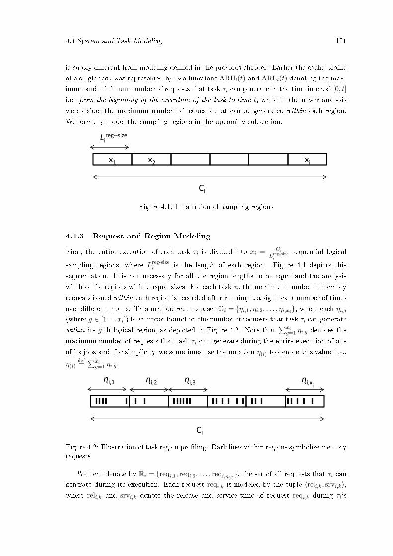
4.1 System and Task Modeling 101
is subtly di�erent from modeling de�ned in the previous chapter: Earlier the cache pro�le
of a single task was represented by two functions ARHi(t) and ARLi(t) denoting the max-
imum and minimum number of requests that task τi can generate in the time interval [0, t]
i.e., from the beginning of the execution of the task to time t, while in the newer analysis
we consider the maximum number of requests that can be generated within each region.
We formally model the sampling regions in the upcoming subsection.
x1 x2 xi
Ci
Lireg--size
Figure 4.1: Illustration of sampling regions
4.1.3 Request and Region Modeling
First, the entire execution of each task τi is divided into xi = CiLreg-sizei
sequential logical
sampling regions, where Lreg-sizei is the length of each region. Figure 4.1 depicts this
segmentation. It is not necessary for all the region lengths to be equal and the analysis
will hold for regions with unequal sizes. For each task τi, the maximum number of memory
requests issued within each region is recorded after running it a signi�cant number of times
over di�erent inputs. This method returns a set Gi = {ηi,1, ηi,2, . . . , ηi,xi}, where each ηi,g(where g ∈ [1 . . . xi]) is an upper bound on the number of requests that task τi can generate
within its g'th logical region, as depicted in Figure 4.2. Note that∑xi
g=1 ηi,g denotes the
maximum number of requests that task τi can generate during the entire execution of one
of its jobs and, for simplicity, we sometimes use the notation η(i) to denote this value, i.e.,
η(i)def=∑xi
g=1 ηi,g.
ɳi,xi
Ci
ɳi,1 ɳi,2
ɳi,3
Figure 4.2: Illustration of task region pro�ling. Dark lines within regions symbolize memoryrequests
We next denote by Ri = {reqi,1, reqi,2, . . . , reqi,η(i)}, the set of all requests that τi cangenerate during its execution. Each request reqi,k is modeled by the tuple 〈reli,k, srvi,k〉,where reli,k and srvi,k denote the release and service time of request reqi,k during τi's
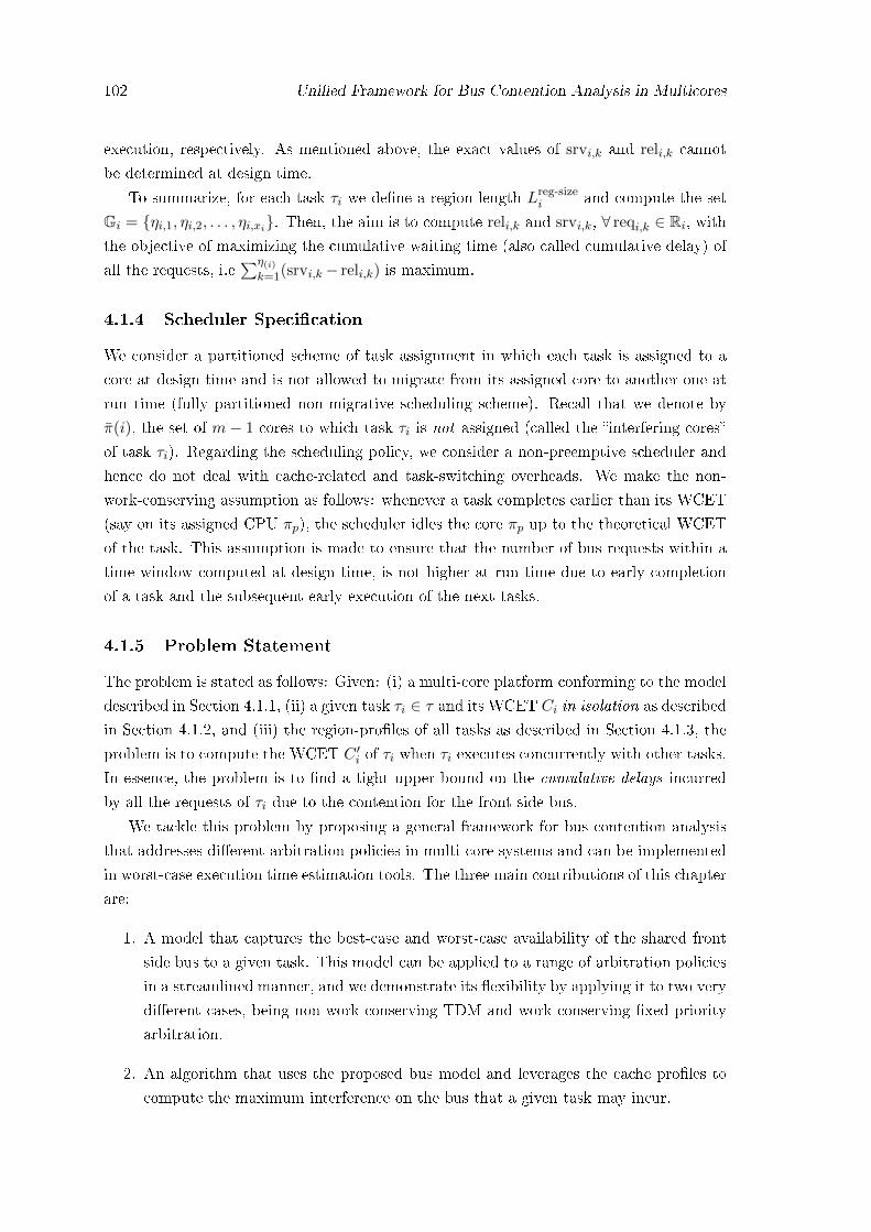
102 Uni�ed Framework for Bus Contention Analysis in Multicores
execution, respectively. As mentioned above, the exact values of srvi,k and reli,k cannot
be determined at design time.
To summarize, for each task τi we de�ne a region length Lreg-sizei and compute the set
Gi = {ηi,1, ηi,2, . . . , ηi,xi}. Then, the aim is to compute reli,k and srvi,k, ∀ reqi,k ∈ Ri, withthe objective of maximizing the cumulative waiting time (also called cumulative delay) of
all the requests, i.e∑η(i)
k=1(srvi,k− reli,k) is maximum.
4.1.4 Scheduler Speci�cation
We consider a partitioned scheme of task assignment in which each task is assigned to a
core at design time and is not allowed to migrate from its assigned core to another one at
run time (fully partitioned non-migrative scheduling scheme). Recall that we denote by
π̄(i), the set of m− 1 cores to which task τi is not assigned (called the �interfering cores�
of task τi). Regarding the scheduling policy, we consider a non-preemptive scheduler and
hence do not deal with cache-related and task-switching overheads. We make the non-
work-conserving assumption as follows: whenever a task completes earlier than its WCET
(say on its assigned CPU πp), the scheduler idles the core πp up to the theoretical WCET
of the task. This assumption is made to ensure that the number of bus requests within a
time window computed at design time, is not higher at run time due to early completion
of a task and the subsequent early execution of the next tasks.
4.1.5 Problem Statement
The problem is stated as follows: Given: (i) a multi-core platform conforming to the model
described in Section 4.1.1, (ii) a given task τi ∈ τ and its WCET Ci in isolation as described
in Section 4.1.2, and (iii) the region-pro�les of all tasks as described in Section 4.1.3, the
problem is to compute the WCET C ′i of τi when τi executes concurrently with other tasks.
In essence, the problem is to �nd a tight upper bound on the cumulative delays incurred
by all the requests of τi due to the contention for the front side bus.
We tackle this problem by proposing a general framework for bus contention analysis
that addresses di�erent arbitration policies in multi-core systems and can be implemented
in worst-case execution time estimation tools. The three main contributions of this chapter
are:
1. A model that captures the best-case and worst-case availability of the shared front
side bus to a given task. This model can be applied to a range of arbitration policies
in a streamlined manner, and we demonstrate its �exibility by applying it to two very
di�erent cases, being non-work-conserving TDM and work-conserving �xed-priority
arbitration.
2. An algorithm that uses the proposed bus model and leverages the cache pro�les to
compute the maximum interference on the bus that a given task may incur.

4.2 Overview of Approach 103
3. A method to tighten the computed bounds and increase the e�ciency and scalability
of the algorithm by splitting the task into smaller sampling regions and leveraging
their cache pro�les.
We experimentally evaluate the proposed approach by applying it to a multi-core COTS
system providing access to a DRAM via a shared bus. The �exibility of the framework is
demonstrated by applying it to di�erent arbiters on a set of applications from the WCET
test suite [111]. We additionally evaluate the accuracy and the run-time of the analysis for
di�erent sample region sizes. Apart from the proof-of-concept by implementation, we also
formally prove the key concepts upon which the algorithm is designed.
The rest of this chapter is organized as follows. An overview of our approach is provided
in Section 4.2. The di�erent steps of our approach are then discussed in detail, starting
with the proposed bus availability model in Section 4.3. We then proceed by showing how
to bound worst-case interference in Sections 4.4 and 4.5, respectively. This is followed by a
method to improve the accuracy and increase the e�ciency of the algorithm, in Section 4.6.
We discuss the related work in Section 4.7. The approach is experimentally evaluated in
Section 4.8 and the chapter is summarized in Section 4.9.
TDM arbiter model
Other arbitration models
Compute Tmin(), Tmax() To model bus availability
Fixed priority Arbiter model
Compute worst-case delay for a Sequence of requests
Algorithm to compute worst-case assignment of requests to slots to
obtain max delay
Arbiter dependent stages
Arbiter independent stages
Work conserving arbiter model
Tighten analysis by using sampling regions
Step 1
Step 2
Step 4
Step 3
Figure 4.3: An overview of the uni�ed framework
4.2 Overview of Approach
Figure 4.3 gives a high-level overview of the approach in arriving at a generalized frame-
work. This section proposes a 4-step approach to solve the aforementioned problem. The
details of each step are later explained in the following sections.

104 Uni�ed Framework for Bus Contention Analysis in Multicores
8
7
6
5
4
3
2
1
Bu
s Sl
ot
Nu
mb
er
Time
TR
Timin(1)
Timin(2)
Timin(3)
Timin(4)
Timin(5)
Timax(1)
Timax(2)
Timax(3)
Timax(4)
Timax(5)
1 2 3 4 5 6 7 8 9 10 Bus slots
TR 2TR 3TR 4TR 5TR 6TR 7TR 8TR 9TR
Figure 4.4: Illustration of Tmaxi (j) and Tmin
i (j)
Step 1: Modeling the availability of the bus
In Section 4.3 we will �rst show how to model the availability of the bus to task τi using
a general model Bi =⟨Tmini (), Tmax
i ()⟩. It is key to note that in the entire analysis that
follows, the bus controller grants access to the bus in units of bus slots, where each bus
slot is of length TR and TR is de�ned as an upper bound on the time to serve a memory
request. Given that several tasks contend for the same shared bus, a given task τi may not
get access to the bus immediately on generating a request (owing to the contention from
co-scheduled tasks from other cores). From now on, we will refer to the bus slots that are
available to τi, as the free bus slots of τi.
De�nition 14. The function Tmini (j) represents the earliest time instant at which the bus
can be available to τi for the j'th time or in other words, the earliest availability of the jth
free bus slot of τi.
De�nition 15. The function Tmaxi (j) represents the latest time instant at which the bus
can be available to τi for the j'th time or in other words, the latest availability of the jth
free bus slot of τi.
The order in which these bus slots are granted to the tasks depend on the arbitration
mechanism; as a consequence it follows that the two functions Tmini (j) and Tmax
i (j) also
depend on the arbitration mechanism as depicted in Figure 4.3. As we shall see in the
next section, for some arbitration policies like Time Division Multiplexing, the availability
of the bus modeled by Tmini (j) and Tmax
i (j) is independent of the tra�c generated by the

4.2 Overview of Approach 105
other cores, while for other arbitration mechanisms like priority based mechanisms, the
interfering requests do in�uence the time at which the analyzed task can avail the bus.
Figure 4.4 illustrates the earliest and the latest times at which a given slot is available
to task τi. As seen in the �gure, the earliest time at which slot 1 may be available to task
τi, Tmini (1) is at time 0, meaning there are no pending requests or task τi is executing in
isolation and there is no contention on the bus. However, as seen, Tmaxi (1) = 5 i.e., τi
may at most have to wait for 4 slots before it can gets a free bus slot and thus can only
be served at the beginning of the �fth slot. Similarly, the availability for the subsequent
slots is depicted in the �gure. Note that this particular example is not representative of
any particular arbitration mechanism.
Step 2: Compute maximum cumulative delay
Given the bus availability model Bi =⟨Tmini (), Tmax
i ()⟩of task τi, we propose a function
to compute the maximum cumulative delay incurred by requests of τi due to contention
on the shared bus. We introduce two concepts in this regard.
De�nition 16. We de�ne a request-to-slot assignment in the context of a single request
by the notation σi(k), which represents that the k'th request generated by τi, i.e., reqi,k is
served in the σi(k)'th bus slot available to task τi.
Similarly, for a sequence of requests we de�ne a mapping as follows.
De�nition 17. We de�ne a request-set mapping Mi = {σi(1), σi(2), . . . , σi(η(i))} to rep-
resent that ∀k ∈ Ri: req,i,k is assigned to σi(k).
We further divide this step is divided in 2 phases
• Given the bus availability model Bi =⟨Tmini (), Tmax
i ()⟩of task τi, its request reqi,k
and a request-to-slot assignment σi(k), we propose a mechanism to compute the
maximum delay that request reqi,k can incur. To do so, we compute the release time
reli,k and service time srvi,k with the objective of maximizing the waiting time (i.e.,
srvi,k− reli,k) of reqi,k.
• In the second phase, given the bus availability model Bi =⟨Tmini (), Tmax
i ()⟩of task τi
and a request-set mapping Mi = {σi(1), σi(2), . . . , σi(η(i))}, we propose a mechanism
to compute the maximum cumulative delay incurred by the set of corresponding
requests. As in the previous phase, assuming a given request-set mapping Mi, we
�nd the release time and service time (reli,k and srvi,k), for all the corresponding
requests with the objective of maximizing the cumulative delay of all these requests.
Determining the values of the release and service times given a request-set mapping is,
however, complicated by the constraints imposed on these variables, such as:

106 Uni�ed Framework for Bus Contention Analysis in Multicores
1. Single outstanding request assumption � For all requests reqi,k, we have reli,k >
srvi,k−1 and
2. Slot availability constraint � A request reqi,k will be served no later than the latest
time instant at which its assigned free bus slot can be available or formally srvi,k ≤Tmaxi (σi(k)).
The proposed mechanism to handle these constraints and �nd the cumulative delay is
discussed in detail in Section 4.4. The focus of Step 2 is how to compute the maximum
cumulative delay for a given mapping and the next step in the analysis ventures into
proposing a technique to arrive at a mapping (among several mappings) for which the
maximum cumulative delay is the largest among the maximum cumulative delays computed
for all feasible mappings.
Step 3: Finding the worst-case request-set mapping
In this step, we propose an algorithm (in Section 4.5) to determine a request-set mapping
Mi for task τi that maximizes the cumulative delay of all its η(i) requests. To do so, our
technique �rst computes an upper bound, UBsloti, on the number of free bus slots that
can possibly be used by task τi. This upper bound gives us a range [1,UBsloti] of free
bus slots within which all the requests of the analyzed task τi will be served. Note that
the number of slots, UBsloti may be much greater than the number of requests to be
served. In that case, a naive approach to maximize the cumulative delay incurred by the
requests of τi is to apply a brute force approach, i.e. all the request-set mappings are
explored and a maximum cumulative delay is computed for each of them by using the
method proposed in Step 2; At the end, only the largest cumulative delay (amongst all
the mappings) is returned. However, such a method does not scale and is computationally
ine�cient due to the exhaustive exploration of all the possible mappings. Therefore, we
reduce the complexity of the problem by eliminating, at an early stage of the analysis, the
request-set mappings that cannot possibly lead to the worst-case delays. This improvement
substantially reduces the time-complexity of the proposed solution.
Step 4: Tightening the analysis using sampling regions
Having shown how to determine the worst request-set mapping in Step 3, and bounding
the maximum cumulative delay for that mapping using the technique explained in Step 2,
there is further scope of tightening the analysis by exploiting the information about the
maximum number of requests in each of the constituent regions of the analyzed task. The
region based analysis helps us to limit the range of the potential free bus slots for a set
of requests. For example, if the k'th request of τi is generated in the g'th region, then
it cannot be served in the j'th free bus slot of τi if Tmaxi (j) < Lreg-size
i × (g − 1), where
Lreg-sizei is the size of the sampling interval. From these constraints, we de�ne a range
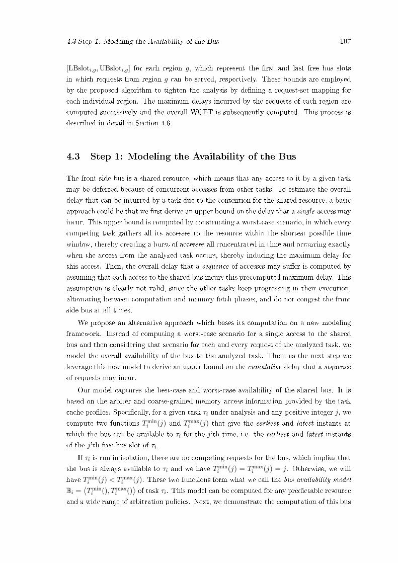
4.3 Step 1: Modeling the Availability of the Bus 107
[LBsloti,g,UBsloti,g] for each region g, which represent the �rst and last free bus slots
in which requests from region g can be served, respectively. These bounds are employed
by the proposed algorithm to tighten the analysis by de�ning a request-set mapping for
each individual region. The maximum delays incurred by the requests of each region are
computed successively and the overall WCET is subsequently computed. This process is
described in detail in Section 4.6.
4.3 Step 1: Modeling the Availability of the Bus
The front side bus is a shared resource, which means that any access to it by a given task
may be deferred because of concurrent accesses from other tasks. To estimate the overall
delay that can be incurred by a task due to the contention for the shared resource, a basic
approach could be that we �rst derive an upper bound on the delay that a single access may
incur. This upper bound is computed by constructing a worst-case scenario, in which every
competing task gathers all its accesses to the resource within the shortest possible time
window, thereby creating a burst of accesses all concentrated in time and occurring exactly
when the access from the analyzed task occurs, thereby inducing the maximum delay for
this access. Then, the overall delay that a sequence of accesses may su�er is computed by
assuming that each access to the shared bus incurs this precomputed maximum delay. This
assumption is clearly not valid, since the other tasks keep progressing in their execution,
alternating between computation and memory fetch phases, and do not congest the front
side bus at all times.
We propose an alternative approach which bases its computation on a new modeling
framework. Instead of computing a worst-case scenario for a single access to the shared
bus and then considering that scenario for each and every request of the analyzed task, we
model the overall availability of the bus to the analyzed task. Then, as the next step we
leverage this new model to derive an upper bound on the cumulative delay that a sequence
of requests may incur.
Our model captures the best-case and worst-case availability of the shared bus. It is
based on the arbiter and coarse-grained memory access information provided by the task
cache pro�les. Speci�cally, for a given task τi under analysis and any positive integer j, we
compute two functions Tmini (j) and Tmax
i (j) that give the earliest and latest instants at
which the bus can be available to τi for the j'th time, i.e. the earliest and latest instants
of the j'th free bus slot of τi.
If τi is run in isolation, there are no competing requests for the bus, which implies that
the bus is always available to τi and we have Tmini (j) = Tmax
i (j) = j. Otherwise, we will
have Tmini (j) < Tmax
i (j). These two functions form what we call the bus availability model
Bi =⟨Tmini (), Tmax
i ()⟩of task τi. This model can be computed for any predictable resource
and a wide range of arbitration policies. Next, we demonstrate the computation of this bus
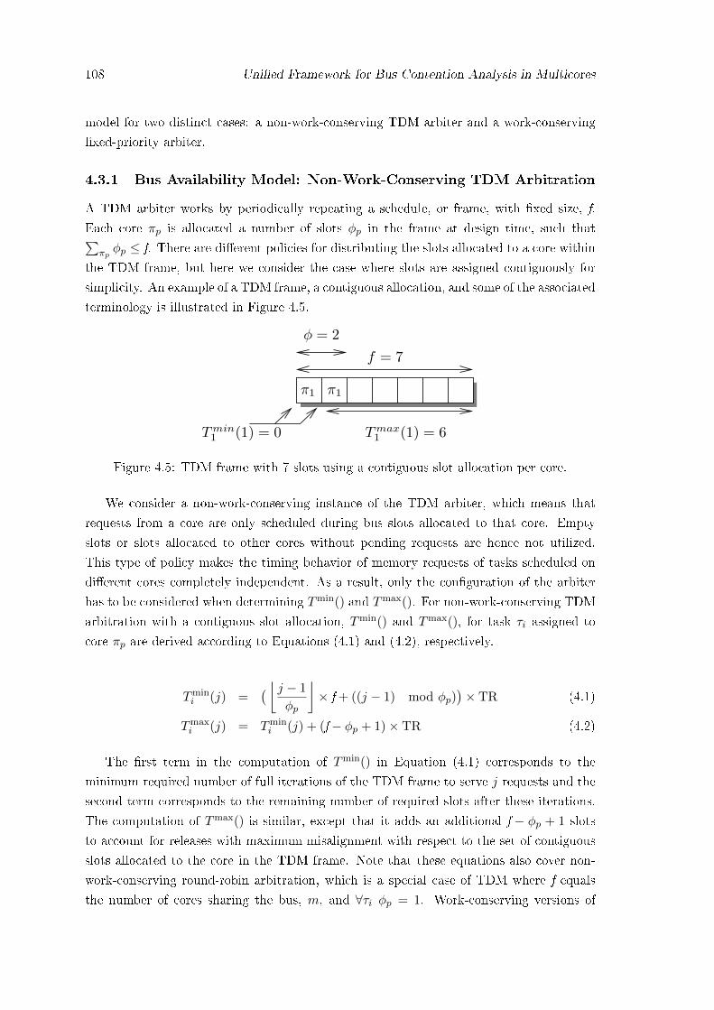
108 Uni�ed Framework for Bus Contention Analysis in Multicores
model for two distinct cases: a non-work-conserving TDM arbiter and a work-conserving
�xed-priority arbiter.
4.3.1 Bus Availability Model: Non-Work-Conserving TDM Arbitration
A TDM arbiter works by periodically repeating a schedule, or frame, with �xed size, f.
Each core πp is allocated a number of slots φp in the frame at design time, such that∑πpφp ≤ f. There are di�erent policies for distributing the slots allocated to a core within
the TDM frame, but here we consider the case where slots are assigned contiguously for
simplicity. An example of a TDM frame, a contiguous allocation, and some of the associated
terminology is illustrated in Figure 4.5.
π1 π1
φ = 2
f = 7
Tmin1 (1) = 0 Tmax
1 (1) = 6
Figure 4.5: TDM frame with 7 slots using a contiguous slot allocation per core.
We consider a non-work-conserving instance of the TDM arbiter, which means that
requests from a core are only scheduled during bus slots allocated to that core. Empty
slots or slots allocated to other cores without pending requests are hence not utilized.
This type of policy makes the timing behavior of memory requests of tasks scheduled on
di�erent cores completely independent. As a result, only the con�guration of the arbiter
has to be considered when determining Tmin() and Tmax(). For non-work-conserving TDM
arbitration with a contiguous slot allocation, Tmin() and Tmax(), for task τi assigned to
core πp are derived according to Equations (4.1) and (4.2), respectively.
Tmini (j) =
( ⌊j − 1
φp
⌋× f + ((j − 1) mod φp)
)× TR (4.1)
Tmaxi (j) = Tmin
i (j) + (f− φp + 1)× TR (4.2)
The �rst term in the computation of Tmin() in Equation (4.1) corresponds to the
minimum required number of full iterations of the TDM frame to serve j requests and the
second term corresponds to the remaining number of required slots after these iterations.
The computation of Tmax() is similar, except that it adds an additional f − φp + 1 slots
to account for releases with maximum misalignment with respect to the set of contiguous
slots allocated to the core in the TDM frame. Note that these equations also cover non-
work-conserving round-robin arbitration, which is a special case of TDM where f equals
the number of cores sharing the bus, m, and ∀τi φp = 1. Work-conserving versions of

4.3 Step 1: Modeling the Availability of the Bus 109
both these arbitration policies can be derived by additionally considering the task cache
pro�les, although this is omitted for brevity. Figure 4.5 graphically illustrates the arrival
times and waiting times corresponding to Tmin1 (1) and Tmax
1 (1). As seen in the �gure, the
Tmin1 (1) = 0, is achieved for a request that arrives just at the beginning of any of the two
slots allocated to its corresponding core and Tmax1 (1) = 6 for a request arriving just after
the last slot allocated to its core has been left idle. For this particular arbitration policy,
the best-case and worst-case arrival with respect to the TDM frame is the same for any
value of j, although this does not hold in general.
4.3.2 Bus Availability Model: Work-Conserving Fixed-Priority Arbitra-
tion
In the context of bus arbitration policies, one of the challenges with currently existing
COTS-based multi-core systems is that the front-side bus does not recognize/respect task
priorities. This is because the bus is generally designed with the aim of enhancing the
average-case performance and is not tailored for real-time systems. This can lead to a
scenario similar to priority inversion in which requests from higher priority tasks are delayed
by requests from lower-priority tasks on the bus. Although the scheduler enforces these
priorities while allocating the processing element (CPU) to tasks, these priorities are not
passed over to the shared hardware resources like the bus and the memory controllers,
which have their own scheduling policies. This problem has been addressed in research by
enabling priorities in priority-driven arbiters to be software programmable directly [112]
or indirectly by tagging each request with its priority [101]. We assume in this section
that the bus is designed according to any of these strategies. Based on this, we design a
bus-availability model for a �xed-priority arbiter.
4.3.2.1 Introducing functions PCRPminq (t) and PCRPmax
q (t)
Assume that the analyzed task τi is scheduled on core πp. In spite of the uncertainty of the
arrival patterns of the requests, it is important to determine a lower and upper bound on
the cumulative number of requests that tasks of a higher priority than the analyzed task τiand scheduled on cores πq 6= πp may inject into the bus. These bounds are denoted by the
PCRPminq (i, t) and PCRPmaxq (i, t) functions. Such bounds can be computed as described
in the previous chapter.
4.3.2.2 Computation of Tmini (j) and Tmax
i (j)
The Tmini (j) and Tmax
i (j) curves represent the earliest and the latest time at which a jth
free bus slot is available to requests of task τi assigned to core πp. When run in isolation,
in the absence of any competing requests for the bus, the bus is always available to τi and
the Tmini (j) and Tmax
i (j) curves merge. Then, the number of interfering requests issued
from core πq 6= πp, can vary between PCRPminq (i, t) and PCRPmax
q (i, t) in a time interval
110 Uni�ed Framework for Bus Contention Analysis in Multicores
of duration t. With this information, we derive the corresponding earliest and the latest
times at which free slots are available to the analyzed task τi assigned to core πp. As stated
earlier, TR is an upper bound on the time to access the memory over the shared front side
bus and each bus slot is of duration TR. Then, we compute Tmini (j) and Tmax
i (j) as:
Tmini (j) = min
t≥0{t|t− (
∑πq 6=πp
PCRPminq (i, t)× TR) = j × TR} (4.3)
Tmaxi (j) = min
t≥0{t|t− (
∑πq 6=πp
PCRPmaxq (i, t)× TR) = j × TR} (4.4)
From the perspective of the analyzed task τi executing on core πp, the bus can be viewed as
resource with two alternating phases: a busy phase, in which it serves the requests from the
other cores and an idle phase which task τi may avail. Equation (4.4) can be interpreted
as follows: Scan the timeline to identify the earliest time instant at which the (continuous
stream of) requests from the other cores (6= πp) have been served and j free slots have
been detected. When the jth slot is free, the time t will exceed the time for servicing the
request (given by the summation term (∑
πq 6=πp PCRPmaxq (i, t)× TR)) by j × TR.
∑πq ≠ πpPCRPmax
q(t)
t
Requests issued by other cores πq ≠ πp
Timax(1) = 7
1 2 3 4 5 6 7 8 9 10 11 12 13 14 15 16 17
Timax(2) = 11 Ti
max(4) = 15
Free bus slot for τi
Figure 4.6: Illustration of computation of Tmaxi (j). Time is expressed in units of TR. Task
τi is assigned to core πp.
Example 1. We illustrate the method of computing Tmaxi (j) with the example illustrated in
Figure 4.6. The �gure represents the cumulative number of requests∑
πq 6=πp PCRPmaxq (i, t)
issued by the other other cores in a period of time t. To clarify∑
πq 6=πp PCRPq(1) = 1,∑πq 6=πp PCRPq(8) = 7,
∑πq 6=πp PCRPq(13) = 10 and so on. Let us compute Tmax
i (4) in
this case. The latest time at which the fourth free bus slot is available to task τi is the �rst
instance, when the time t exceeds the total number of requests issued by the other cores in
time t by 4. This happens in the example at time 15 where the cumulative requests at time
15 is 11. And hence Tmaxi (4) = 15.
As seen in this section, the Tmini (j) and Tmax
i (j) functions are arbitration dependent
and can be computed for di�erent arbiters (TDM, round-robin, �xed-priority and FIFO

4.4 Step 2: Find the maximum cumulative delay for a given request-set mapping 111
(omitted here)). They serve as an input to the next blocks of the proposed framework
that compute the increased execution time based on the model. In contrast, the methods
described in the following sections are independent of the arbitration mechanism.
4.4 Step 2: Find the maximum cumulative delay for a given
request-set mapping
In this section, we �rst describe a method to compute the maximum waiting time, given
a single request, a free bus slot assignment to that request and the bus availability model.
The same rationale is then extended to compute the cumulative waiting time for a sequence
of requests of a given task in conformance to certain constraints. For a given request-to-slot
assignment, the key idea to maximize the waiting time of that request is to release it as
early as possible and delay its servicing to the latest possible time. In other words, for the
given free bus slot σi(k) we need to determine a lower bound on the release time of request
reqi,k, an upper bound on its service time of a request for the given slot and then compute
the resulting maximum waiting time. A set of lemmas are provided below as foundations
to this central theme.
Property 2. By construction, Tmaxi (1) is the longest waiting time for one request before
it can be assigned a free bus slot.
In order to compute Tmaxi (1), the maximum tra�c that all the potentially competing
tasks can generate in order to fully occupy the system bus is computed (recall the task
packing algorithm). For non-fair bus arbitration schemes, this means that the �rst request
of the analyzed task may be served after all pending requests from other tasks. The
subsequent requests of the analyzed task may incur an equal or lesser waiting time than
that incurred by the �rst request. In this respect, Tmaxi (1) represents the longest waiting
time for a given request.
4.4.1 Maximum delay for a single request-to-slot assignment
We now proceed in Lemmas 1 and 2 by lower bounding the release time of a request and
upper bounding the service time to enable the computation of its maximum delay.
Lemma 1 (A lower bound on the release time of a request). For any task τi ∈ τ and for
all k > 1, let reqi,k−1 and reqi,k be two consecutive requests generated by τi. For a given
request-to-slot assignment σi(k − 1) and σi(k), if request reqi,k−1 has been served at time
srvi,k−1 in the σi(k − 1)'th free bus slot then it holds that
reli,k ≥ max(Tmini (σi(k)− 1) + 1, srvi,k−1 +(σi(k)− σi(k − 1)) ∗ TR) (4.5)
Proof. The lemma is based on two simple observations:
112 Uni�ed Framework for Bus Contention Analysis in Multicores
1. The earliest time of releasing a request is in the scenario when it is released immedi-
ately after the earliest time instant at which the bus can be free for the (σi(k)−1)'th
time. Otherwise the request would have been served in the previous available free
slot, (σi(k)− 1). Formally, reli,k ≥ Tmini (σi(k)− 1) + 1, and more importantly,
2. A request can only be released after the previous request is served i.e. reli,k ≥ srvi,k−1.
In addition, for it to be served in slot σi(k), all the intermediate slots between the slot
occupied by the previous request must be occupied and not available to τi. This gets us
to the term reli,k ≥ srvi,k−1 +(σi(k)− σi(k− 1) ∗TR). In order to satisfy both conditions,
the maximum of the resulting values is considered.
Lemma 2 (An upper bound on the service time of a request). For any task τi ∈ τ and for
all k > 1, if request reqi,k is served at time srvi,k in the σi(k)'th free bus slot then it holds
that
srvi,k ≤ min(Tmaxi (σi(k)), reli,k +Tmax
i (1)) (4.6)
Proof. The latest time at which a request reqi,k assigned to slot σi(k) is served is Tmaxi (σi(k))
(by de�nition). Since Tmaxi (1) denotes the maximum delay that a request may su�er, the
value of srvi,k should not be greater than reli,k +Tmaxi (1). Equation (4.6) upholds these
two conditions by considering the minimum of the respective values.
The maximum delay for servicing the given request k in slot σi(k) is then given by
srvi,k− reli,k.
4.5 Step 3: Finding the worst-case assignment
4.5.1 Maximum cumulative delay for a request-set mapping
In the previous section, we established a method to compute an upper bound on the delay
of a single request and a given slot assignment for that request. Now, we extend this
result to maximize the cumulative delay of a sequence of requests, given a request-set
mapping Mi = {σi(1), . . . , σi(η(i))}. To maximize the cumulative delay for the mapping
Mi, we compute the individual maximum delay for each request by applying the lemmas
described in Section 4.4.1. Since the release time (and thus the delay) of a given request
reqi,k is dependent on the service time srvi,k−1 of the previous one (see Equation (4.5)), we
start by computing the maximum delay of the �rst request reqi,1 and iterate up to request
reqi,η(i) . We show in Lemma 3 that this iterative process leads to a worst-case delay.
Lemma 3 (Worst-case cumulative delay). Let Mi = {σi(1), . . . , σi(η(i))} refer to a request-set mapping for the η(i) requests of task τi. Let Di(k) be the maximum cumulative delay
for the �rst k requests {reqi,1, reqi,2, . . . reqi,k}, given this mapping Mi and ∆k = (σi(k)−

4.5 Step 3: Finding the worst-case assignment 113
σi(k − 1)) ∗ TR . Then the delay, Di(η(i)) =∑η(i)
k=1 srvi,k− reli,k of all these requests is
maximized for:
reli,k =
Tmini (σi(k)− 1) + 1 if k = 1
max(Tmini (σi(k)− 1) + 1, srvi,k−1 +∆k) otherwise
(4.7)
srvi,k = min(Tmaxi (σi(k)), reli,k +Tmax
i (1)) (4.8)
Proof. We prove the lemma by induction. First, we show in the basic step that the claim
is true considering only the �rst request reqi,1 and its slot assignment σi(1). That is, we
show that the release and service times given by Equations 4.7 and 4.8 result in a maxi-
mum cumulative delay Di(1) = srvi,1− reli,1. Then, in the inductive step, we show that if
the claim is true considering the set of the �rst k requests, k ≥ 1 (induction hypothesis),
then the property holds for the �rst (k + 1) requests as well. In other words, assuming
that Equations 4.7 and 4.8 assign a release and service time to the k �rst requests that
result in a maximum cumulative delay Di(k), then the same equations provide a maximum
cumulative delay Di(k + 1) when applied to the �rst (k + 1) requests. Both the basic and
inductive steps are proven by showing that any other choice of release and service time, for
any of the requests in the considered set of requests, results in a lower cumulative delay.
In order to ease the reading of the proof, we shall make use of Figure 4.7 which depicts
di�erent cases, as well as the notations used in the proof.
Basic step. By considering only the �rst request reqi,1, it is easy to see that any release
time reli,1 di�erent from that given by Equation 4.7 leads to reli,1 > Tmini (σi(1)− 1) + 1.
This follows from the fact that having reli,1 < Tmini (σi(1)−1) + 1 is not possible, as shown
in Lemma 1. Besides, choosing any other release time reli,1 > Tmini (σi(1) − 1) + 1 would
have as sole impact, a decrease in the di�erence (srvi,1− reli,1), and subsequently a lower
delay Di(1) incurred by request reqi,1. In short, since Tmini (σi(1)− 1) + 1 is a lower bound
on the release time of request reqi,1 (from Lemma 1), choosing reli,1 = Tmini (σi(1)− 1) + 1
is the best choice to guarantee a maximum delay for the �rst request. Similarly, since
min(Tmaxi (σi(k)), reli,k +Tmax
i (k)) was shown to be an upper bound on the service time of
request reqi,k, ∀k (see Lemma 2), it is easy to see that the choice of srvi,1 by Equation (4.8)
also guarantees a maximum delay for this �rst request.
In conclusion, we showed that Di(1) = srvi,1− reli,1 is maximum when reli,1 and srvi,1
are given by the equations of Lemma 3.
Inductive step. Assuming that Equations 4.7 and 4.8 de�ne a release and a service
time for the �rst k requests of τi such that their cumulative delay Di(k) is maximized, we
will show that de�ning reli,k+1 and srvi,k+1 using the equations of Lemma 3 maximizes
Di(k+ 1). By applying the same reasoning as in the basic step, it is evident that choosing

114 Uni�ed Framework for Bus Contention Analysis in Multicores
Figure 4.7: Illustration of the three cases 1, 2 and 3 of Lemma 3.
any other value of reli,k+1 greater than its lower bound (given in Lemma 1 and Eq. (4.7))
and/or any other service time srvi,k+1 lower than its upper bound (given in Lemma 2 and
Equation (4.8)) induces a lower delay for request reqi,k+1, and thus a lower cumulative
delay Di(k + 1).
However, it may be noted from the release-time equation (Eq. 4.7) that the choice of
service time srvi,k of the previous request reqi,k in�uences the lower bound on reli,k+1, and
subsequently an upper bound on srvi,k+1 (see Equation (4.8)). One should therefore inves-
tigate the following question: although choosing srvi,k = min(Tmaxi (σi(k)), reli,k +Tmax
i (1))
guarantees a maximum cumulative delay Di(k) for the �rst k requests (from the induction
hypothesis), doing so might de�ne a range of possible values for reli,k+1 that discards those
leading to a maximum cumulative delay Di(k + 1). The remainder of this proof consists
in showing that any value of srvi,k di�erent from that given by Equation (4.8) results in a
lower cumulative delay Di(k + 1).
To �gure out how srvi,k a�ects the range of possible values for reli,k+1 and srvi,k+1, let us
consider di�erent values X and Y for srvi,k, where X = min(Tmaxi (σi(k)), reli,k +Tmax
i (1))
(as given by Expression (4.8)) and Y is any positive number < X. An example of X and
Y is depicted in Figure 4.7 (note that in this example, we have X = reli,k +Tmaxi (1)). We
show in the following that Di(k + 1) is always maximum for srvi,k = X.
We �rst introduce two notations for compaction and readability: ∆k+1 and Q1. Let
∆k+1 = (σi(k + 1) − σi(k)) ∗ TR and Q1 = Tmini (σi(k + 1) − 1) + 1. We know from
Lemma 1, reli,k+1 ≥ max(Tmini (σi(k + 1)− 1) + 1, srvi,k +∆k+1 and thus three cases may
arise depending the bus-slot assignment σi(k + 1) of request reqi,k+1:
1. Q1 ≤ Y + ∆k+1 < X + ∆k+1

4.5 Step 3: Finding the worst-case assignment 115
2. Y + ∆k+1 < Q1 ≤ X + ∆k+1
3. Y + ∆k+1 ≤ X + ∆k+1 ≤ Q1
Case 1. Q1 ≤ Y + ∆k+1 < X + ∆k+1
In this case, choosing srvi,k = Y leads to reli,k+1 ≥ Y + ∆k+1 (from Lemma 1). By setting
reli,k+1 to Y + ∆k+1, we get
Di(k + 1) =k+1∑`=1
(srvi,`− reli,`)
=
k−1∑`=1
(srvi,`− reli,`) + (srvi,k− reli,k) + (srvi,k+1− reli,k+1)
=
k−1∑`=1
(srvi,`− reli,`) + Y − reli,k + srvi,k+1−(Y + ∆k+1)
=k−1∑`=1
(srvi,`− reli,`) + srvi,k+1− reli,k−∆k+1
(4.9)
On the other hand, choosing srvi,k = X leads to reli,k+1 ≥ X + ∆k (from Lemma 1).
If we choose reli,k+1 = X + ∆k+1 (i.e., the earliest possible release time) then applying the
same reasoning as above leads to the same equality, i.e.,
Di(k + 1) =k−1∑`=1
(srvi,`− reli,`) + srvi,k+1− reli,k−∆k+1 (4.10)
Since (4.9) = (4.10), we can claim that choosing srvi,k = X leads to a worst-case cumulative
delay Di(k + 1).
Case 2. Y + ∆k+1 < Q1 ≤ X + ∆k+1
In this case, choosing srvi,k = Y leads to reli,k+1 ≥ Tmin(σi(k + 1)− 1) (from Lemma 1).
Let reli,k+1 = Tmini (σi(k + 1)− 1)) (i.e., the earliest possible release time-instant), from a
reasoning similar to that above it holds that
Di(k + 1) =k+1∑`=1
(srvi,`− reli,`)
=
k−1∑`=1
(srvi,`− reli,`) + Y − reli,k + srvi,k+1−Q1
<k−1∑`=1
(srvi,`− reli,`) + Y − reli,k + srvi,k+1−(Y + ∆k+1)
<k−1∑`=1
(srvi,`− reli,`)− reli,k + srvi,k+1−∆k+1
(4.11)
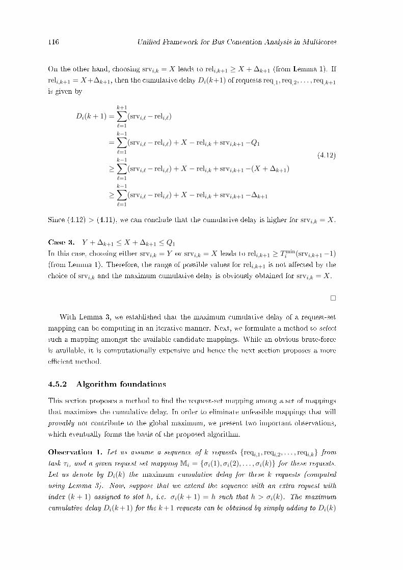
116 Uni�ed Framework for Bus Contention Analysis in Multicores
On the other hand, choosing srvi,k = X leads to reli,k+1 ≥ X + ∆k+1 (from Lemma 1). If
reli,k+1 = X+∆k+1, then the cumulative delayDi(k+1) of requests req,1, req
,2, . . . , req,k+1
is given by
Di(k + 1) =
k+1∑`=1
(srvi,`− reli,`)
=k−1∑`=1
(srvi,`− reli,`) +X − reli,k + srvi,k+1−Q1
≥k−1∑`=1
(srvi,`− reli,`) +X − reli,k + srvi,k+1−(X + ∆k+1)
≥k−1∑`=1
(srvi,`− reli,`) +X − reli,k + srvi,k+1−∆k+1
(4.12)
Since (4.12) > (4.11), we can conclude that the cumulative delay is higher for srvi,k = X.
Case 3. Y + ∆k+1 ≤ X + ∆k+1 ≤ Q1
In this case, choosing either srvi,k = Y or srvi,k = X leads to reli,k+1 ≥ Tmini (srvi,k+1−1)
(from Lemma 1). Therefore, the range of possible values for reli,k+1 is not a�ected by the
choice of srvi,k and the maximum cumulative delay is obviously obtained for srvi,k = X.
With Lemma 3, we established that the maximum cumulative delay of a request-set
mapping can be computing in an iterative manner. Next, we formulate a method to select
such a mapping amongst the available candidate mappings. While an obvious brute-force
is available, it is computationally expensive and hence the next section proposes a more
e�cient method.
4.5.2 Algorithm foundations
This section proposes a method to �nd the request-set mapping among a set of mappings
that maximizes the cumulative delay. In order to eliminate unfeasible mappings that will
provably not contribute to the global maximum, we present two important observations,
which eventually forms the basis of the proposed algorithm.
Observation 1. Let us assume a sequence of k requests {reqi,1, reqi,2, . . . , reqi,k} from
task τi, and a given request-set mapping Mi = {σi(1), σi(2), . . . , σi(k)} for these requests.
Let us denote by Di(k) the maximum cumulative delay for these k requests (computed
using Lemma 3). Now, suppose that we extend the sequence with an extra request with
index (k + 1) assigned to slot h, i.e. σi(k + 1) = h such that h > σi(k). The maximum
cumulative delay Di(k+1) for the k+1 requests can be obtained by simply adding to Di(k)

4.5 Step 3: Finding the worst-case assignment 117
the maximum delay for that last request reqi,k+1. This maximum delay can be obtained
using Lemma 3 by assuming only the service time of the kth request that was obtained
during the computation of Di(k).
Observation 2. If a sequence of (k + 1) requests are served within a range [1, h] of free
bus slots, then the maximum cumulative delay for these (k + 1) requests is the maximum
between the largest delay computed by assuming
C1. the (k + 1) requests are all served within the range [1, h] of free bus slots, and
C2. the �rst k requests are served within the range slot [1, h − 1] and request (k + 1) is
served in slot h.
Based on these observations, we construct a method to compute Di(k) from Di(k− 1),
∀k, which ultimately yields Di(η(i)). The method is shown in Algorithm 5 and an expla-
nation of its operation is given below. Note that this algorithm is �safe-by-construction�
as it computes Di(η(i)) by investigating all possible assignments of these η(i) requests to
free bus slots (only those assignments that are proven unfeasible are discarded).
4.5.3 Algorithm Description
The request-set mappings are captured in a two-dimensional array with η(i) rows and
UBsloti columns. The input to the algorithm is the number of requests of the analyzed
task τi, and an upper bound on the available slots, UBsloti in which the η(i) requests
may be served. Note that the variables k and j are used to refer to requests and slots,
respectively. Each cell c(k, j) of this array holds a list of tuples ek,j = 〈Di(k), σi(k), srvi,k〉,where each tuple ek,j in that list re�ects a feasible assignment of the �rst k requests to k
free bus slots within the range [1, j]. The members of this tuple denote:
• the maximum delay Di(k) that can be obtained with the corresponding assignment,
• the free bus slot in which the k'th request has been served to reach that maximum
delay Di(k), i.e. σi(k) ∈ [k, j], and
• the corresponding time srvi,k at which that k'th request has been served in that slot.
The algorithm proceeds in a row-wise manner, by assigning the �rst request reqi,1 to
all feasible slots and computing the cumulative delays and then proceeding to analyze the
second request (next row of the array) and so on. For the �rst request and �rst slot, the
algorithm computes the worst-case delay when the �rst request is assigned to the �rst free
bus slot (Lines 7, 9, 10, and 11). To do so, it uses Lemma 3 and adds the corresponding
tuple e1,1 to the list of cell c(1, 1), in this case e1,1 = 〈Tmaxi (1), 1, Tmax
i (1)〉. The list
contains only this tuple.
For k = 1 and j > 1, the algorithm computes all the maximum delays by considering
every assignment of the �rst request, reqi,1, to free bus slots ≤ j. First, the list of the
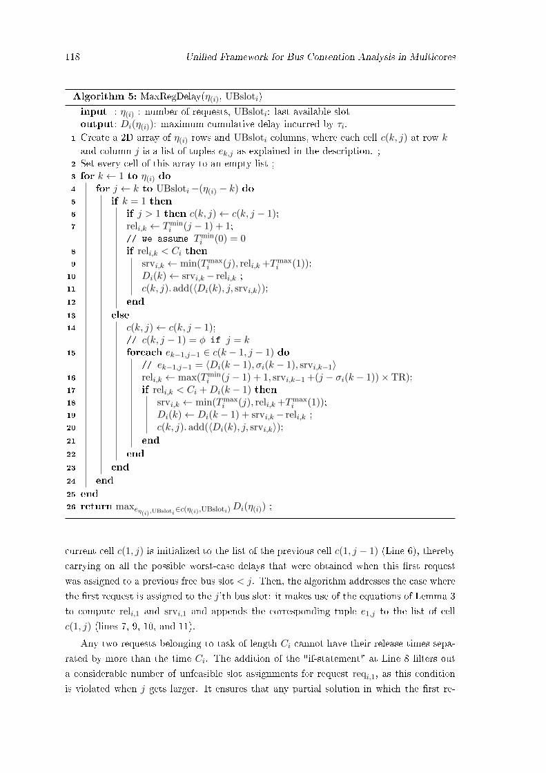
118 Uni�ed Framework for Bus Contention Analysis in Multicores
Algorithm 5: MaxRegDelay(η(i), UBsloti)
input : η(i) : number of requests, UBsloti: last available slotoutput: Di(η(i)): maximum cumulative delay incurred by τi.
1 Create a 2D array of η(i) rows and UBsloti columns, where each cell c(k, j) at row k
and column j is a list of tuples ek,j as explained in the description. ;2 Set every cell of this array to an empty list ;3 for k ← 1 to η(i) do
4 for j ← k to UBsloti−(η(i) − k) do
5 if k = 1 then6 if j > 1 then c(k, j)← c(k, j − 1);7 reli,k ← Tmin
i (j − 1) + 1;// we assume Tmin
i (0) = 08 if reli,k < Ci then9 srvi,k ← min(Tmax
i (j), reli,k +Tmaxi (1));
10 Di(k)← srvi,k− reli,k ;11 c(k, j). add(〈Di(k), j, srvi,k〉);12 end
13 else14 c(k, j)← c(k, j − 1);
// c(k, j − 1) = φ if j = k15 foreach ek−1,j−1 ∈ c(k − 1, j − 1) do
// ek−1,j−1 = 〈Di(k − 1), σi(k − 1), srvi,k−1〉16 reli,k ← max(Tmin
i (j − 1) + 1, srvi,k−1 +(j − σi(k − 1))× TR);17 if reli,k < Ci +Di(k − 1) then18 srvi,k ← min(Tmax
i (j), reli,k +Tmaxi (1));
19 Di(k)← Di(k − 1) + srvi,k− reli,k ;20 c(k, j). add(〈Di(k), j, srvi,k〉);21 end
22 end
23 end
24 end
25 end26 return maxeη(i),UBsloti
∈c(η(i),UBsloti)Di(η(i)) ;
current cell c(1, j) is initialized to the list of the previous cell c(1, j − 1) (Line 6), thereby
carrying on all the possible worst-case delays that were obtained when this �rst request
was assigned to a previous free bus slot < j. Then, the algorithm addresses the case where
the �rst request is assigned to the j'th bus slot: it makes use of the equations of Lemma 3
to compute reli,1 and srvi,1 and appends the corresponding tuple e1,j to the list of cell
c(1, j) (lines 7, 9, 10, and 11).
Any two requests belonging to task of length Ci cannot have their release times sepa-
rated by more than the time Ci. The addition of the "if-statement" at Line 8 �lters out
a considerable number of unfeasible slot assignments for request reqi,1, as this condition
is violated when j gets larger. It ensures that any partial solution in which the �rst re-
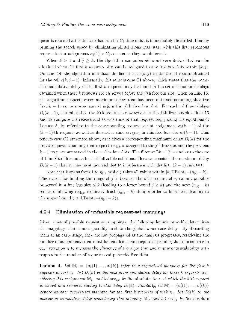
4.5 Step 3: Finding the worst-case assignment 119
quest is released after the task has run for Ci time units is immediately discarded, thereby
pruning the search space by eliminating all solutions that start with this �rst erroneous
request-to-slot assignment σi(1) > Ci as soon as they are detected.
When k > 1 and j ≥ k, the algorithm computes all worst-case delays that can be
obtained when the �rst k requests of τi can be assigned to any free bus slots within [k, j].
On Line 14, the algorithm initializes the list of cell c(k, j) to the list of results obtained
for the cell c(k, j− 1). Informally, this re�ects case C1 above, which states that the worst-
case cumulative delay of the �rst k requests may be found in the set of maximum delays
obtained when these k requests are all served before the j'th free bus slot. Then on Line 15,
the algorithm inspects every maximum delay that has been obtained assuming that the
�rst k − 1 requests were served before the j'th free bus slot. For each of these delays
Di(k − 1), assuming that the k'th request is now served in the j'th free bus slot, lines 16
and 18 compute the release and service time of that request reqi,k using the equations of
Lemma 3, by referring to the corresponding request-to-slot assignment σi(k − 1) of the
(k − 1)'th request, as well as its service time srvi,k−1 in this free bus slot σi(k − 1). This
re�ects case C2 presented above, as it gives a corresponding maximum delay Di(k) for the
�rst k requests assuming that request reqi,k is assigned to the jth free slot and the previous
k− 1 requests are served in the earlier bus slots. The �lter at Line 17 is similar to the one
at Line 8 to �lter out a host of infeasible solutions. Here we consider the maximum delay
Di(k − 1) that τi may have incurred due to interference with the �rst (k − 1) requests.
Note that k spans from 1 to η(i), while j takes all values within [k,UBsloti−(η(i)−k)].
The reason for limiting the range of j is because the k'th request of τi cannot possibly
be served in a free bus slot ≤ k (leading to a lower bound j ≥ k) and the next (η(i) − k)
requests following reqi,k require at least (η(i) − k) slots in order to be served (leading to
the upper bound j ≤ UBsloti−(η(i) − k)).
4.5.4 Elimination of unfeasible request-set mappings
Given a set of possible request-set mappings, the following lemma provably determines
the mappings that cannot possibly lead to the global worst-case delay. By discarding
them at an early stage, they are not propagated as the analysis progresses, restricting the
number of assignments that must be handled. The purpose of pruning the solution tree in
each iteration is to increase the e�ciency of the algorithm and improve its scalability with
respect to the number of requests and potential free slots.
Lemma 4. Let Mi = {σi(1), . . . , σi(k)} refer to a request-set mapping for the �rst k
requests of task τi. Let Di(k) be the maximum cumulative delay for these k requests con-
sidering this assignment Mi, and let srvi,k be the absolute time at which the k'th request
is served in a scenario leading to this delay Di(k). Similarly, let M′i = {σ′i(1), . . . , σ′i(k)}denote another request-set mapping for the �rst k requests of task τi. Let D′i(k) be the
maximum cumulative delay considering this mapping M′i, and let srv′i,k be the absolute

120 Uni�ed Framework for Bus Contention Analysis in Multicores
time at which the k'th request is served in a scenario leading to this delay D′i(k). If it holds
that
σi(k) ≤ σ′i(k) (4.13)
and Di(k) ≤ D′i(k) (4.14)
and srvi,k +(σ′i(k)− σi(k))× TR ≥ srv′i,k (4.15)
then for all h > σ′i(k), assigning an extra request reqi,k+1 to the h'th free bus slot in both
mappings Mi and M′i, i.e., σi(k + 1) = σ′i(k + 1) = h, leads to
σi(k + 1) = σ′i(k + 1) (4.16)
and Di(k + 1) ≤ D′i(k + 1) (4.17)
and srvi,k+1 +(σ′i(k + 1)− σi(k + 1))× TR ≥ srv′i,k+1 (4.18)
The vital inference from the above observations is that the maximum cumulative delay for
the �rst (k+1) requests of τi is higher, and the service time of the (k+1)'th request smaller,
by using the mapping M′i for the �rst k requests (instead of the mapping Mi). Note that
since Conditions (4.16), (4.17), and (4.18) are the same as (4.13), (4.14), and (4.15), the
lemma continues to hold for all the subsequent requests > k + 1.
Proof. From the claim itself, Equation (4.16) trivially holds (we stated this equality only
for completeness, in order to show that the situation after assigning the (k+ 1)'th request
is same as the situation before assigning it). Let us start the proof by introducing some
notations for readability:
C1 = Tmini (h− 1) + 1 and C2 = Tmax
i (h)
and ∆k = (h− σi(k))× TR and ∆′k = (h− σ′i(k))× TR
According to these notations and from the equations of Lemma 3, the four quantities
srvi,k+1, reli,k+1, srv′i,k+1, and rel′i,k+1 can be re-written as
reli,k+1 = max(C1, srvi,k +∆k) (4.19)
srvi,k+1 = min(C2, reli,k+1 +Tmaxi (1)) (4.20)
rel′i,k+1 = max(C1, srv′i,k +∆′k) (4.21)
srv′i,k+1 = min(C2, rel′i,k+1 +Tmaxi (1)) (4.22)
According to (4.15), we have
srv′i,k−σ′i(k) ≤ srvi,k−σi(k)

4.5 Step 3: Finding the worst-case assignment 121
and thus
srv′i,k +h− σ′i(k) ≤ srvi,k +h− σi(k)
which gives
srv′i,k +∆′k ≤ srvi,k +∆k (4.23)
Therefore, regarding Inequalities (4.17) and (4.18), we have three cases to investigate.
• Case 1: srv′i,k +∆′k ≤ srvi,k +∆k ≤ C1.
• Case 2: srv′i,k +∆′k ≤ C1 ≤ srvi,k +∆k.
• Case 3: C1 ≤ srv′i,k +∆′k ≤ srvi,k +∆k.
Case 1: srv′i,k +∆′k ≤ srvi,k +∆k ≤ C1.
In this case, we have from (4.19) and (4.21), reli,k+1 = rel′i,k+1 = C1 and from (4.20)
and (4.22), srvi,k+1 = srv′i,k+1 , which satis�es (4.18) since σi(k + 1) = σ′i(k + 1) = h.
Since reli,k+1 = rel′i,k+1 and srvi,k+1 = srv′i,k+1 , using Di(k) ≤ D′i(k) from (4.14), we
get
Di(k) + srvi,k+1− reli,k+1 ≤ D′i(k) + srv′i,k+1− rel′i,k+1
and then,
Di(k + 1) ≤ D′i(k + 1)
which satis�es (4.17).
Case 2: srv′i,k +∆′k ≤ C1 ≤ srvi,k +∆k.
In this case, we get from (4.19) and (4.21),
reli,k+1 = srvi,k +∆k ≥ rel′i,k+1 = C1 (4.24)
Next, we need to handle the relation between the service times srvi,k+1 and srv′i,k+1 and
we have to explore three sub-cases.
• Case 2.1: rel′i,k+1 +Tmaxi (1) ≤ reli,k+1 +Tmax
i (1) ≤ C2.
• Case 2.2: rel′i,k+1 +Tmaxi (1) ≤ C2 ≤ reli,k+1 +Tmax
i (1).
• Case 2.3: C2 ≤ rel′i,k+1 +Tmaxi (1) ≤ reli,k+1 +Tmax
i (1).
Case 2.1: rel′i,k+1 +Tmaxi (1) ≤ reli,k+1 +Tmax
i (1) ≤ C2.
From (4.20) and (4.22) we get
srvi,k+1 = reli,k+1 +Tmaxi (1) (4.25)
srv′i,k+1 = rel′i,k+1 +Tmaxi (1) (4.26)

122 Uni�ed Framework for Bus Contention Analysis in Multicores
From (4.24), (4.25) and (4.26), it immediately follows that srvi,k+1 ≥ srv′i,k+1, which
satis�es (4.18) since σi(k + 1) = σ′i(k + 1) = h. Also from (4.25) and (4.26), it holds that
srvi,k+1− reli,k+1 = Tmaxi (1) = srv′i,k+1− rel′i,k+1. Using Di(k) ≤ D′i(k) from (4.14), we
get
Di(k) + Tmaxi (1) ≤ D′i(k) + Tmax
i (1)
and then
Di(k) + srvi,k+1− reli,k+1 ≤ D′i(k) + srv′i,k+1− rel′i,k+1
This implies
Di(k + 1) ≤ D′i(k + 1)
which satis�es (4.17).
Case 2.2: rel′i,k+1 +Tmaxi (1) ≤ C2 ≤ reli,k+1 +Tmax
i (1).
From (4.20) and (4.22), we get srvi,k+1 = C2 and srv′i,k+1 = rel′i,k+1 +Tmaxi (1). We thus
get srvi,k+1 ≥ srv′i,k+1, which satis�es (4.18) since σi(k + 1) = σ′i(k + 1) = h. Then, if
Inequality (4.17) is not satis�ed we must have:
Di(k + 1) > D′i(k + 1)
and thus,
Di(k) + srvi,k+1− reli,k+1 > D′i(k) + srv′i,k+1− rel′i,k+1
By replacing srvi,k+1 and srv′i,k+1 with their values, we get
Di(k) + C2 − reli,k+1 > D′i(k) + Tmaxi (1)
and then,
Di(k) > D′i(k) + Tmaxi (1)− (C2 − reli,k+1)
and since from the case C2 − reli,k+1 ≤ Tmaxi (1), it holds from the above inequality that
Di(k) > D′i(k)
which contradicts (4.14). This contradiction implies that Equation 4.17 is satis�ed.
Case 2.3: C2 ≤ rel′i,k+1 +Tmaxi (1) ≤ reli,k+1 +Tmax
i (1).
From (4.20) and (4.22), we get srvi,k+1 = srv′i,k+1 = C2 and it immediately follows that
srvi,k+1 ≥ srv′i,k+1, which satis�es (4.18) since σi(k + 1) = σ′i(k + 1) = h. Then, if
Inequality (4.17) is not satis�ed we must have:
Di(k + 1) > D′i(k + 1)
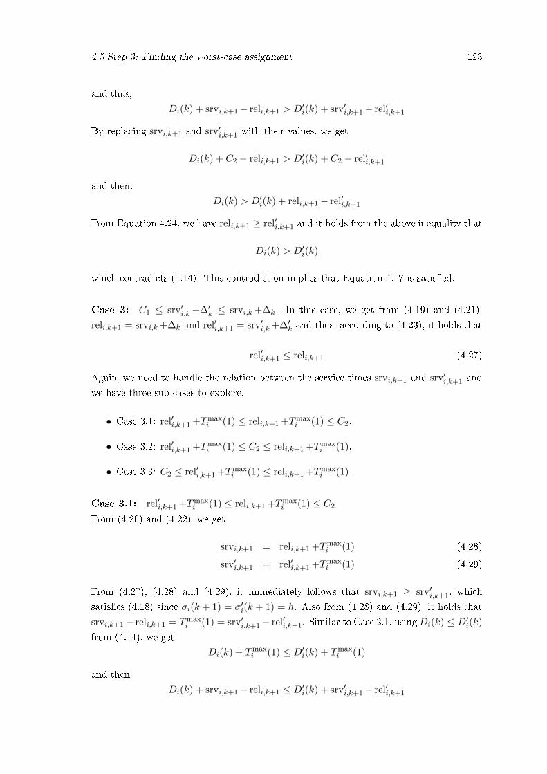
4.5 Step 3: Finding the worst-case assignment 123
and thus,
Di(k) + srvi,k+1− reli,k+1 > D′i(k) + srv′i,k+1− rel′i,k+1
By replacing srvi,k+1 and srv′i,k+1 with their values, we get
Di(k) + C2 − reli,k+1 > D′i(k) + C2 − rel′i,k+1
and then,
Di(k) > D′i(k) + reli,k+1− rel′i,k+1
From Equation 4.24, we have reli,k+1 ≥ rel′i,k+1 and it holds from the above inequality that
Di(k) > D′i(k)
which contradicts (4.14). This contradiction implies that Equation 4.17 is satis�ed.
Case 3: C1 ≤ srv′i,k +∆′k ≤ srvi,k +∆k. In this case, we get from (4.19) and (4.21),
reli,k+1 = srvi,k +∆k and rel′i,k+1 = srv′i,k +∆′k and thus, according to (4.23), it holds that
rel′i,k+1 ≤ reli,k+1 (4.27)
Again, we need to handle the relation between the service times srvi,k+1 and srv′i,k+1 and
we have three sub-cases to explore.
• Case 3.1: rel′i,k+1 +Tmaxi (1) ≤ reli,k+1 +Tmax
i (1) ≤ C2.
• Case 3.2: rel′i,k+1 +Tmaxi (1) ≤ C2 ≤ reli,k+1 +Tmax
i (1).
• Case 3.3: C2 ≤ rel′i,k+1 +Tmaxi (1) ≤ reli,k+1 +Tmax
i (1).
Case 3.1: rel′i,k+1 +Tmaxi (1) ≤ reli,k+1 +Tmax
i (1) ≤ C2.
From (4.20) and (4.22), we get
srvi,k+1 = reli,k+1 +Tmaxi (1) (4.28)
srv′i,k+1 = rel′i,k+1 +Tmaxi (1) (4.29)
From (4.27), (4.28) and (4.29), it immediately follows that srvi,k+1 ≥ srv′i,k+1, which
satis�es (4.18) since σi(k + 1) = σ′i(k + 1) = h. Also from (4.28) and (4.29), it holds that
srvi,k+1− reli,k+1 = Tmaxi (1) = srv′i,k+1− rel′i,k+1. Similar to Case 2.1, usingDi(k) ≤ D′i(k)
from (4.14), we get
Di(k) + Tmaxi (1) ≤ D′i(k) + Tmax
i (1)
and then
Di(k) + srvi,k+1− reli,k+1 ≤ D′i(k) + srv′i,k+1− rel′i,k+1

124 Uni�ed Framework for Bus Contention Analysis in Multicores
This implies
Di(k + 1) ≤ D′i(k + 1)
which satis�es (4.17).
Case 3.2: rel′i,k+1 +Tmaxi (1) ≤ C2 ≤ reli,k+1 +Tmax
i (1).
From (4.20) and (4.22) we get srvi,k+1 = C2 and srv′i,k+1 = rel′i,k+1 +Tmaxi (1). We thus
get srvi,k+1 ≥ srv′i,k+1, which satis�es (4.18) since σi(k + 1) = σ′i(k + 1) = h. Then, if
Inequality (4.17) is not satis�ed we must have:
Di(k + 1) > D′i(k + 1)
and thus,
Di(k) + srvi,k+1− reli,k+1 > D′i(k) + srv′i,k+1− rel′i,k+1
By replacing srvi,k+1 and srv′i,k+1 for their values, we get
Di(k) + C2 − reli,k+1 > D′i(k) + Tmaxi (1)
and then,
Di(k) > D′i(k) + Tmaxi (1)− (C2 − reli,k+1)
and since from the case C2 − reli,k+1 ≤ Tmaxi (1), it holds from the above inequality that
Di(k) > D′i(k)
which contradicts (4.14). This contradiction implies that Equation 4.17 is satis�ed.
Case 3.3: C2 ≤ rel′i,k+1 +Tmaxi (1) ≤ reli,k+1 +Tmax
i (1).
From (4.20) and (4.22), we get srvi,k+1 = srv′i,k+1 = C2 and it immediately follows that
srvi,k+1 ≥ srv′i,k+1, which satis�es (4.18) since σi(k + 1) = σ′i(k + 1) = h. Then, if
Inequality (4.17) is not satis�ed we must have:
Di(k + 1) > D′i(k + 1)
and thus,
Di(k) + srvi,k+1− reli,k+1 > D′i(k) + srv′i,k+1− rel′i,k+1
By replacing srvi,k+1 and srv′i,k+1 for their values, we get
Di(k) + C2 − reli,k+1 > D′i(k) + C2 − rel′i,k+1
and then,
Di(k) > D′i(k) + reli,k+1− rel′i,k+1

4.6 Step 4: Region-Wise Analysis 125
From Equation (4.27), we have reli,k+1 ≥ rel′i,k+1 and therefore its holds from the above
inequality that
Di(k) > D′i(k)
which contradicts (4.14). This contradiction implies that Equation 4.17 is satis�ed.
In order to leverage the result of Lemma 4, we can add a function ListReduce(c(k, j))
at the end of the �rst inner loop, i.e., �for j ← k to UBsloti−(η(i) − k)� in Algo. 5. This
function makes sure that @ two distinct tuples e1k,j and e
2k,j in the list of c(k, j)) such that
σi(k)1 ≤ σi(k)2
Di(k)1 ≤ Di(k)2
srv1i,k +(σi(k)2 − σi(k)1) ≥ srv2
i,k
Each time such a pair of tuples is found, only the tuple e2k,j is kept and the tuple e1
k,j is
discarded. This is a key addition to the algorithm that signi�cantly reduces the number of
tuples in c(k, j)). We later return to experimentally evaluate the bene�ts of this elimination
in Section 4.8.
4.6 Step 4: Region-Wise Analysis
As seen in Section 4.1.3, we can obtain more information on the distribution of requests by
dividing the execution of each task into a sequence of sampling regions. For each region,
we can derive a lower and upper bound on the number of requests that can be issued by
the task within that region. However Algorithm 5 did not leverage this region-speci�c
information and used only a coarser grain information about the number of requests in the
entire task, represented by η(i). In other words, Algorithm 5 views the input task τi as a
single region that can issue up to η(i) requests. As a consequence, the resulting analysis
may lead to a pessimistic upper bound as illustrated in the following example.
Example 2. As a simple example, consider that a task issues 10 requests and there are
500 potential free slots, such that slots numbered [491 to 500] contribute to the 10 highest
delays. Then a single-region based approach will assign all the 10 requests to slots [491 to
500]. Next, assume we break the task into 2 regions and �nd that there are 7 requests in
Region 1 and 3 requests in Region 2. Likewise, we also compute that the �rst 300 slots are
feasibly available for region 1 and the next 200 slots are available for Region 2. It can be
seen that the previous mapping will lead to conservative estimates. The resulting analysis
can be made tighter with this information of request distributions and slot availability, since
with this information, the algorithm will assign the 7 requests to the slots (with the 7 highest
delays) from these 300 slots and the 3 requests to 3 slots from 491 to 500.
Although the exact intervals of the arrivals of these requests are di�cult to discern, if
it is possible to divide the task into regions and derive an upper bound on the number of

126 Uni�ed Framework for Bus Contention Analysis in Multicores
Figure 4.8: Notations used in proof of Lemma 5
requests that can be generated in each region, then likewise we can �nd an upper bound
on the range of slots that can be potentially available to the requests of a given region. In
the absence of such demarcations, requests may be assigned to unfeasible slots, leading to
pessimistic outcomes.
Thus, the advantage of region-based analysis is two-fold: Firstly, they decrease the com-
putation time by limiting the number of possible candidate slots that must be explored
and secondly, they lead to tighter analysis by discarding a considerable amount of infeasi-
ble mappings. We proceed by elaborating on the theoretical foundations of region-based
analysis, followed by a detailed description of the algorithm.
4.6.1 Theoretical Foundation
When a task is divided into regions and runs in conjunction with other tasks, the time at
which each of its regions starts executing depends on the delays incurred by the requests
issued in its previous regions. The following lemmas express the relation that exist between
the starting time of a region and the maximum delay that it can incur. These properties
allow for a �ne-tuned WCET analysis in which the distribution of requests across regions
is exploited to obtain region-accurate estimates.
Lemma 5. Consider two execution scenarios of a task τi of region g. In the �rst scenario,
region g starts executing at time t1, whereas in the second scenario region g starts executing
at time t2 and t1 < t2. It may happen that the maximum delay that region g can possibly
incur in Scenario 1 is higher than the delay incurred in Scenario 2.
Proof. We prove the claim by using a simple example. Let us consider the functions Tmini (·)
and Tmaxi (·) depicted in Figure 4.8 and assume that ηi,g = 2. By starting at time t2 the
maximum delay that region g can incur is given by ∆2 + ∆3 while it can be seen that, by
starting at time t1, the maximum delay is ∆1 + ∆2 > ∆2 + ∆3.
Lemma 6. Although Lemma 5 holds and the delay incurred by beginning the execution
at time t1 may be greater than the delay incurred at time t2 (> t1), the �nishing time of
region g can never be higher if the task begins to executes at time t1. Informally, the extra
delay that region g may incur in Scenario 1 by starting earlier does not make up for the
di�erence of starting time between the two scenarios.

4.6 Step 4: Region-Wise Analysis 127
Scenario 1:
Scenario 2:
Scenario 3:
Figure 4.9: Notations used in proof of Lemma 6
Proof. The proof is obtained by contradiction. Let us denote by f1 and f2 the �nishing
time of region g in Scenario 1 and 2, respectively. By contradiction, assume that f1 > f2.
Figure 4.9 illustrates these two scenarios: an �X� represents the release of a request, a
continuous line represents the execution of the region, and a dashed line is an interval of
time during which the task stalls, waiting for a request to be served. It is assumed in this
illustration that region g generates a maximum of ηi,g = 4 requests.
Let D1 and D2 denote the maximum delay that region g can incur in Scenarios 1
and 2, respectively. There are two cases: if D1 ≤ D2, we have f1 = t1 + Lreg-sizei + D1
and f2 = t2 + Lreg-sizei +D2 and since t1 < t2, it holds that f1 < f2, which contradicts our
assumption. Otherwise, if D1 > D2, suppose that region g incurs the maximum delay of
(t2− t1) during the time-interval [t1, t2], with a single request generated upon beginning its
execution. The delay incurred by this single request can even extend until time t3 > t2, as
depicted in Scenario 1 of Figure 4.9. This scenario can easily be shown to be a worst case
(with respect to the �nishing time), as it generates the maximum delay with the fewest
requests, thereby delaying the actual workload of Lreg-sizei units of execution as much as
possible.
Now, let us denote by {σi(2), . . . , σi(ηi,g)} the request-set mapping of the (ηi,g − 1)
last requests of region g in Scenario 1 (note that, unlike what is depicted on Figure 4.9,
the mapping of these requests may be the same as in Scenario 2). We can create a third
scenario, in which region g starts its execution at time t2 (as in Scenario 2) and such that
the �rst request is released upon beginning its execution, thereby incurring the same delay
between [t2, t3] as in Scenario 1, and all the subsequent requests follow the same free-bus-
slot assignment as in Scenario 1, thereby incurring again the same delay as in Scenario 1.
In this new Scenario 3, it thus holds that region g starts at time t2 and �nishes at time
f3 = t2 +D3 = f1 > f2 = t2 +D2, which contradicts our initial assumption de�ning D2 as
the maximum delay that region g can incur when starting at time t2.
To summarize, an important inference from Lemma 6 is that the WCET of a task
(considering contention) can be determined by computing the worst-case �nishing time f1

128 Uni�ed Framework for Bus Contention Analysis in Multicores
of its �rst region, and then iterating over the subsequent regions, assuming for each region
g, a starting time of fg−1. The WCET of the entire task is then given by the worst-case
�nishing time of its last region.
4.6.2 Description of the Algorithm for Region-Based Analysis
Algorithm 6: ComputeTaskWCET(τi, Tmini (.), Tmax
i (.))
input : τi,Tmini (.), Tmax
i (.)output: WCET of τi (considering contention)
1 wi = CiLreg-sizei
; C ′i ← 0 ;
2 for region g in task τi from 1 to wi do3 ηi,g ← No of requests in region g ;4 UBTimei,g ← fi,g−1 + Lreg-size
i + ηi,g ∗ Tmaxi (1);
// with fi,0 = 05 LBsloti,g ← minx>0{x | Tmax
i (g) ≥ fi,g−1};6 UBsloti,g ← minx>0{x | Tmin
i (g) ≥ UBTimei,g};7 δi,g = MaxRegDelay(ηi,g,LBsloti,g,UBsloti,g);8 fi,g = fi,g−1 + Lreg-size
i + δi,g ;9 end
10 return fi,wi ;
With Algorithm 6, we propose an arbiter-independent method to determine the worst-
case cumulative delay. It is basically an extension of Algorithm 5 and augments it with
region-based information Since the inputs to this algorithm are the Tmini (.), Tmax
i (.) func-
tions and the details of the analyzed task, any arbiter for which these values can be
determined can leverage this algorithm.
The algorithm commences by computing the number wi of regions (Line 1) and then
considers each region g successively (Line 2). Next, given the number ηi,g of requests
in the analyzed region g, it �nds a coarse upper bound on its increased execution time
UBTimei,g assuming that each request in region g may incur a delay of Tmaxi (1). Then, it
computes the range of the free bus slots that the requests of region g may occupy (Lines
5-6), assuming on Line 5 a starting time of fi,g−1.
To compute the worst-case delay of each region, the algorithm invokes a slightly modi-
�ed version of Algorithm 5 in which (i) j now spans from g+LBsloti,g to UBsloti,g −(ηi,g−g)) on Line 4, (ii) the 2D array contains UBsloti,g −LBsloti,g columns, (iii) all the refer-
ences to a cell c(k, j) are replaced with a reference to cell c(k, j − LBsloti,g), and (iv)
references to Ci are substituted for references to Lreg-sizei . Note that a task modeled as a
single region is a special case in which LBsloti,1 = 1, the region size Lreg-sizei is Ci, and
the maximum number of requests is η(i). The delay of the currently analyzed region δi,g
4.7 Related Work 129
is computed on Line 7 and is then accounted for in the worst-case �nishing time fi,g com-
puted on Line 8. The process is repeated for all the regions and the �nishing time of the
last region gives the increased WCET of the task.
4.7 Related Work
Bus contention analysis has received considerable attention in recent years and these e�orts
can be classi�ed into two classes: 1) approaches that modify the hardware or the software
of the system to enable or improve analysis, and 2) approaches that analyze a given system.
We proceed by discussing each of these in turn.
On the hardware side, a number of memory controllers have been designed speci�cally
for real-time systems and proposed together with corresponding analyses that bound the
WCRT of memory requests [57, 59, 58, 113, 114]. These analyses bene�t from full knowl-
edge of the internals of the memory controller, such as page policies, transaction scheduler
and the DRAM command scheduler, and exploit this information to produce tight bounds.
On the software side, servers with memory budgets, built into the operating system, have
been proposed to limit the memory interference [115, 116] from tasks executing on other
cores, enabling it to be bounded based on enforcement rather than characterization. Our
work contrasts to these e�orts in the sense that it targets COTS platforms and considers
both the software and hardware to be given.
Several approaches have been proposed for bus contention analysis in given COTS
platforms. Similarly to our work, most analyses consider multi-core systems with a bus
providing access to a shared memory with a single port [80, 106, 79, 91, 117]. However,
these works are quite di�erent with respect to the considered task models and scheduling
policies for both the tasks themselves and their memory requests. Applications are typically
modeled as independent periodic/sporadic task sets or acyclic task graphs [90, 73], and the
scheduling is often based on �xed-priorities [91, 106], while tasks in task graphs are statically
scheduled using techniques that respect precedence constraints, e.g. list scheduling. The
approaches support di�erent task preemption models, ranging from fully preemptive [80,
106] to non-preemptive [91, 117, 90, 73], and with limited-preemption at the granularity
of TDM time slots as a compromise in between [79].
A problem with most of the previously mentioned analysis approaches is that they only
support a single bus arbiter, such as any work-conserving arbiter [91, 80], �xed-priority
arbitration, round robin [117], TDM [90, 73, 74, 75, 76] or �rst-come �rst-served. This
does not address the diversity of memory arbiters in COTS platforms, making them point
solutions exclusive to a single platform rather than a reusable framework that applies more
generally. This problem is partially mitigated by the analysis in [79] that supports three of
these arbitration mechanisms in a single uni�ed framework, although this work is limited to
systems where periodic tasks are modeled as sets of superblocks and scheduled using TDM.
In contrast, our work is more general as it applies to any sporadic constrained-deadline

130 Uni�ed Framework for Bus Contention Analysis in Multicores
tasks under any non-preemptive task scheduler. To conclude, this work presents a scalable
framework for bus contention analysis that is more general than previous work for COTS-
based non-preemptive real-time systems with respect to supported task schedulers and
memory arbiters.
4.8 Experimental Results
This section experimentally evaluates the proposed framework by simulating a multi-core
system running real application traces. First, the experimental setup is explained, followed
by an experiment that demonstrates the generality of our approach by executing the ap-
plications with three di�erent arbiters and evaluating the accuracy and run-time of the
proposed analysis. Lastly, we experiment with di�erent region sizes and show how �ner-
grained task region-pro�les improve accuracy and increase the e�ciency of the analysis.
4.8.1 Experimental Setup
The hardware platform in our experiments is based on the SimpleScalar 3.0 processor
simulator [118] with separate data and instruction caches, each with a size of 16 KB. The L2
cache is a private uni�ed 128 KB cache with 128 B cache lines and an associativity of 4. The
processor core is assumed to run at a frequency of 1.6 GHz. The memory device corresponds
to a 64-bit DDR3-1600 DIMM [119] running at a frequency of 800 MHz, meaning that one
memory cycle equals two processor cycles. The memory access time TR = 80 processor
cycles for a request of 128 B, corresponding to an in-order DRAM scheduler with limited
pipelining of requests. This setup is similar to contemporary COTS-platforms, such as
Freescale P4080. The experiments consider a platform instance with 4 cores, each core
running an application from the WCET test suite [111] as a single independent task.
For each application in the benchmark, memory-trace �les were generated by running
it on the experimental platform. The traces were �nally post-processed according to the
sampling regions used in the experiments to compute the region-pro�les of the task. Similar
experiments were also carried out for the ChStone [107] benchmarks.
4.8.2 Application to Di�erent Arbitration Mechanisms
The objective of this experiment is to demonstrate the generality of our approach by apply-
ing it to three commonly used arbiters, being �xed-priority, an unspeci�ed work-conserving
arbiter, and TDM, respectively. For each task, we determine the interference from other
tasks and compute the increase in WCET for each of the three arbiters using a region size
of 2000 cycles. We also examine the run-time of the proposed analysis for the di�erent ar-
biters. To get a representative sample of applications for the WCET benchmark, we chose
the two most memory-intensive (minmax and lcdnum) and the two least memory-intensive
(lms and adpcm) applications. The results of the experiment are shown in Figure 4.10,
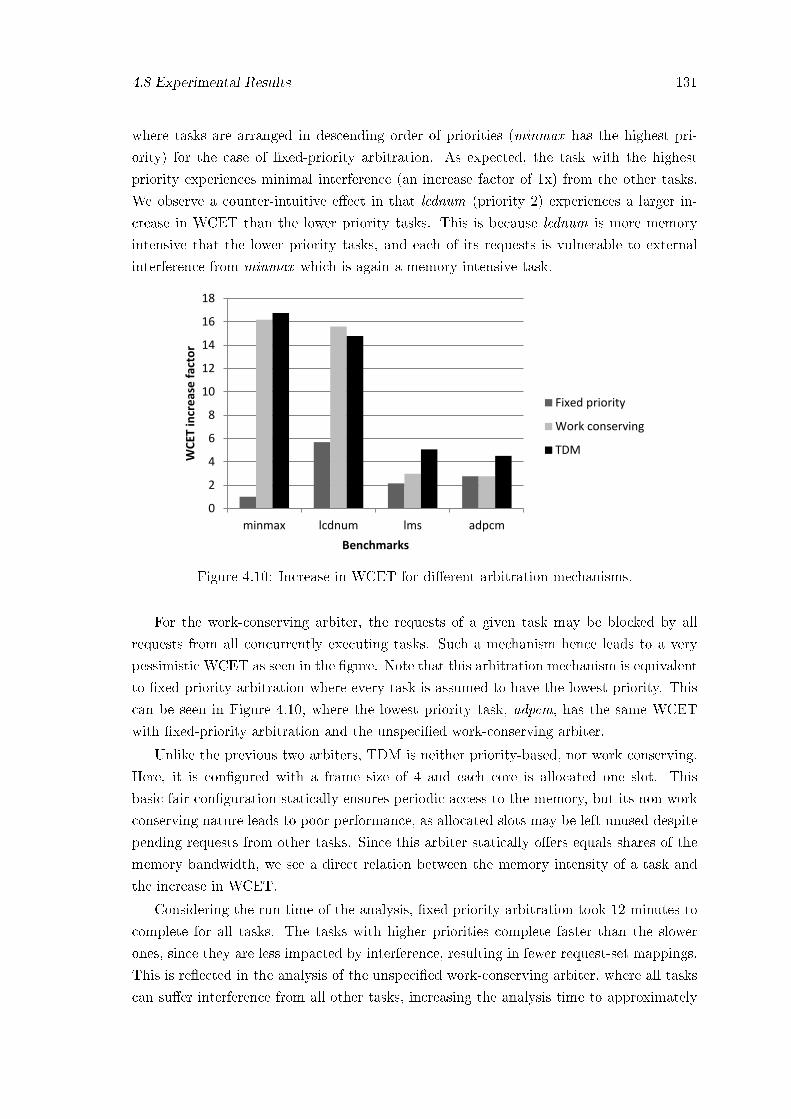
4.8 Experimental Results 131
where tasks are arranged in descending order of priorities (minmax has the highest pri-
ority) for the case of �xed-priority arbitration. As expected, the task with the highest
priority experiences minimal interference (an increase factor of 1x) from the other tasks.
We observe a counter-intuitive e�ect in that lcdnum (priority 2) experiences a larger in-
crease in WCET than the lower priority tasks. This is because lcdnum is more memory
intensive that the lower priority tasks, and each of its requests is vulnerable to external
interference from minmax which is again a memory intensive task.
0
2
4
6
8
10
12
14
16
18
minmax lcdnum lms adpcm
WC
ET in
cre
ase
fac
tor
Benchmarks
Fixed priority
Work conserving
TDM
Figure 4.10: Increase in WCET for di�erent arbitration mechanisms.
For the work-conserving arbiter, the requests of a given task may be blocked by all
requests from all concurrently executing tasks. Such a mechanism hence leads to a very
pessimistic WCET as seen in the �gure. Note that this arbitration mechanism is equivalent
to �xed-priority arbitration where every task is assumed to have the lowest priority. This
can be seen in Figure 4.10, where the lowest priority task, adpcm, has the same WCET
with �xed-priority arbitration and the unspeci�ed work-conserving arbiter.
Unlike the previous two arbiters, TDM is neither priority-based, nor work conserving.
Here, it is con�gured with a frame size of 4 and each core is allocated one slot. This
basic fair con�guration statically ensures periodic access to the memory, but its non-work
conserving nature leads to poor performance, as allocated slots may be left unused despite
pending requests from other tasks. Since this arbiter statically o�ers equals shares of the
memory bandwidth, we see a direct relation between the memory intensity of a task and
the increase in WCET.
Considering the run-time of the analysis, �xed-priority arbitration took 12 minutes to
complete for all tasks. The tasks with higher priorities complete faster than the slower
ones, since they are less impacted by interference, resulting in fewer request-set mappings.
This is re�ected in the analysis of the unspeci�ed work-conserving arbiter, where all tasks
can su�er interference from all other tasks, increasing the analysis time to approximately

132 Uni�ed Framework for Bus Contention Analysis in Multicores
35 minutes. In contrast, the TDM arbiter is non-work-conserving and thereby completely
independent of other tasks, enabling the computation of Tmini (.) and Tmax
i (.) in constant
time. Furthermore, small TDM frame sizes provide relatively few possible request-set map-
pings, reducing the total analysis time to less than 5 minutes. While running the analysis,
we further-more instrumented the algorithm to evaluate the bene�ts of the optimization
proposed in Section 4.5 (List reduction). The result of this evaluation showed that the
hit-ratio ranged from 20-40% (with an average of 30%), which considerably reduces the
run-time for cases where the number of candidate slots is very high.
0
2
4
6
8
10
12
14
lcdnum lms adpcm
WC
ET In
cre
ase
fac
tor
Benchmarks
1000
2000
3000
5000
Figure 4.11: Increase in WCET for di�erent region sizes (in cycles).
4.8.3 Impact of Region Size
We conclude by experimentally evaluating the impact of the region size. To this end, we re-
ran the previous experiments with the �xed-priority arbiter using both smaller and larger
region sizes. Four di�erent sizes are used: 1000, 2000, 3000 and 5000 cycles, respectively,
where larger region sizes imply fewer regions and coarser-grained cache pro�les for each
region. The results of the experiment are shown in Figure 4.11. Note that the highest
priority task, minmax, is not shown in the �gure, as it su�ers the same negligible inter-
ference across all region sizes. For the other tasks, the results con�rm the intuition that
smaller regions result in tighter WCET, since �ner-grained task region pro�les eliminate
a lot of uncertainty. In terms of run-time of the analysis, the results re�ect that smaller
region sizes imply fewer candidate slots, reducing run-time. To quantify this claim, the
total analysis time was 4, 12, 34 and 125 minutes for region sizes of 1k, 2k ,3k and 5k
cycles, respectively.

4.9 Conclusion 133
4.9 Conclusion
In this chapter we developed a framework to compute the worst-case execution time of
a task which can work for di�erent arbitration mechanisms. By using the tools for task
and core pro�ling developed in the previous chapter, we proposed a method to model the
availability of the bus to a given task and leveraged this model further to compute the
increased delay that the task incurs when co-scheduled with other tasks contending on the
bus. The proposed algorithm presented a general interface into which di�erent arbiters
can be seamlessly plugged to compute the resulting WCET. We also demonstrated the
applicability of our framework for two di�erent arbiters: a non-work-conserving TDM
arbiter and work-conserving �xed-priority arbiter. In the next chapter, we will explore
another component � the memory controller and look into its inner workings.

134 Uni�ed Framework for Bus Contention Analysis in Multicores

Chapter 5
Bus Contention Analysis of Phase
Change Memory based Multicores
If the facts don't �t the theory, change the facts.
Albert Einstein
5.1 Introduction to Phase Change Memory
A key development in the embedded systems arena is the adoption of the multicore technol-
ogy as their core processing platform. Another research trend now in memory technology
is to �nd a single memory for both temporary storage and permanent storage in per-
sonal computers as well as embedded systems. The goal is the uni�cation of memory,
to avoid having a separate SRAM, DRAM and �ash. An interesting viable option is the
possibility of adopting Phase Change Memory (PCM) as main memory for embedded sys-
tems [120, 26, 104, 121, 103]. Phase change memory (PCM) is an emerging non-volatile
solid-state memory technology employing materials that change states or phases. These
materials are among the most ubiquitous materials in information storage, as they are
already mass-deployed in rewritable optical discs such as CDs and DVDs. PCM leverages
the signi�cant change in electrical resistivity when the material changes between its two
states i.e the amorphous and crystalline phases. The material has high electrical resistivity
in its amorphous state and low resistivity in its crystalline state � corresponding to the 1
and 0 states of binary data.
PCM has been positioned to complement or replace existing volatile memories like
Dynamic Random Access Memory (DRAM) as the main memory and as a potential al-
ternative to FLASH memory. PCM is more power e�cient than DRAM because it is
non-volatile and therefore unlike DRAM does not need periodic refreshes. The experts
from Ovonyx [26] state that:
135

136 Bus Contention Analysis of Phase Change Memory based Multicores
�PCM can displace a signi�cant amount of DRAM in both mobile and PC/server applica-
tions. PCM today already o�ers a cell size smaller than DRAM and with PCM's inherent
enhanced scalability over DRAM, the cost advantage of PCM will increase with time. As
more volatile DRAM is displaced by non-volatile PCM, signi�cant power savings will be re-
alized, providing extended battery life in mobile applications and signi�cantly reduced power
consumption in PC and server applications. Initially, PCM will not be targeted as a direct
replacement for all DRAM, but rather to displace a large percentage of DRAM in applica-
tions that don't require the in�nite DRAM cycle endurance and can bene�t the most from
the dramatically reduced power consumption of PCM.�
Challenges in adoption: In spite of the aforementioned bene�ts, its adoption for real-
time embedded systems is not without its own challenges: its read latency is acceptable but
the write latency is very high. While DRAM read and write latencies are in the range of
20-50ns, PCM read latency is of the order of 50ns while the write latency is of the order of
0.5�1µs [122]. With such high latencies, from the real-time context, many tasks on systems
with PCM-based memory (without any modi�cations) may miss their deadlines or incur
unacceptable delays in their execution times [101]. To address this issue, researchers have
proposed PCM memory controller scheduling policies and designs that overcome these
challenges, facilitating its adoption in real-time systems [104, 101]. From the architecture
side, increasing the cache sizes can also mitigate the penalties associated with the high write
latencies. Researchers have also envisioned and architected a multi-tiered vertical memory
hierarchy which consists of the on-chip caches, an o�-chip DRAM memory and then a PCM
main memory as the last memory level. Another problem of PCM is its limited endurance
(up to 108 writes), which can be mitigated with a large dedicated on-chip cache (SRAM or
embedded DRAM) that can absorb most of the write misses � PCM-only memories then
become feasible with the advantage of energy e�ciency and density.
Our work focuses on developing a mechanism to aid the timing analysis of real-time
embedded systems hosted on multicores systems with PCM as the main memory.
5.1.1 Problem overview and contributions
To ensure at design time that real-time embedded applications deliver the required func-
tionality within pre-set time limits, bounds on key parameters like the worst-case execution
time (WCET) must be established. In this chapter, we build upon the state-of-the-art
methods that compute these WCET estimates, and address the problem of extending such
upper bounds considering the contention for the PCM memory controller and the asym-
metric read and write latencies. We assume a multicore system with private caches and a
PCM-based main memory system.
Main contributions The currently existing analysis techniques to compute the delay
due to contention on the shared memory do not consider the request handling mechanisms
5.2 Related Work 137
within the memory controller and treat it as a black box. A �xed latency for servicing read
and write memory requests is typically assumed in the analysis, which is appropriate for
DRAM based memory systems. However, given the substantial di�erence in the time to
service a read and write request, the above assumptions may lead to unsafe or pessimistic
estimates. A new memory scheduling policy proposed by contemporary researchers Zhou
et.al [101] considering PCM's read/write timing asymmetries reduces the number of dead-
line misses and makes it practical to deploy real-time applications. This work builds on the
work of Zhou et.al and provides the timing analysis for PCM main memories in multicore
systems.
1. We believe that this is the �rst work to derive the increased WCET of a task consid-
ering asymmetric-latency based systems and the memory request scheduling policy
within the realm of real-time systems. Although this particular analysis focuses on
PCM, it could be used for other memory technologies with asymmetric read and
write latencies like Spin Transfer Torque (STT) memories.
2. In this work, we propose a method to model the arrival and servicing of the requests
in the PCM memory controller considering the memory scheduling policy.
3. We leverage the model to compute the increased WCET of a task considering the
contention on the bus and the memory controller. Our method exploits the memory
request pro�le of the analyzed tasks in order to tighten the WCET.
4. The analysis is then validated by running our proposed method on benchmarks from
MediaBench [123]. A set of experiments have been performed to highlight the impact
of other parameters like the nature of co-scheduled tasks and the task priorities on
the WCET.
The rest of the chapter is organized as follows: Section 5.2 discusses the related work
in the area of timing analysis and PCM. The system model is described in Section 5.3. An
initial basic approach is proposed in Section 5.4, followed by Section 5.5 which describes
our new method. This method is validated and the results are presented in Section 5.6.
The chapter �nally concludes in Section 5.7.
5.2 Related Work
5.2.1 Earlier work on PCM
PCM has been proposed as a promising candidate for energy-e�cient main memory sys-
tems. Lee et al. [124] propose area-neutral bu�er organizations and partial write tech-
niques to mitigate the negative impacts of PCM's long latencies, high energy and limited
endurance. Qureshi et al. [125] propose a hybrid architecture that uses a DRAM cache to
�lter accesses to PCM. The hybrid architecture has the latency bene�ts of DRAM and the

138 Bus Contention Analysis of Phase Change Memory based Multicores
capacity and scalability advantages of PCM. Ferreira et al. [126] study page partitioning
in the DRAM cache to reduce the amount of data written back to PCM. Zhou et al. [127]
propose PCM as a direct replacement for DRAM in main memory without bu�er organi-
zation. Zhang et al. [128] present a hybrid PCM/DRAM memory architecture that uses
a small DRAM as write bu�er. OS-level paging scheme is applied to improve PCM write
performance and lifetime.
Researchers have also proposed techniques for mitigating the impact of undesirable
PCM characteristics. As mentioned above, bu�er organizations [126, 124, 125, 128] are ef-
fective to hide the impacts of slow PCM writes (compared to DRAM). Techniques like write
cancellation and write pausing [129] have also been proposed to improve the performance
of PCM reads by delaying the extremely slow write operations.
PCM controller modi�cations to make it real-time friendly Given the high delays
for servicing write requests, many tasks executing on a system with the basic PCM memory
system can experience deadline misses. To overcome this issue, Zhou et.al [101] proposed
three main features to be integrated into the PCM memory controller, which resulted in
substantially reducing the number of tasks that missed their deadlines.
1. Ability to attach external priorities to each memory request, together with the type
of the request (read or write) and its arrival time. Priorities are assigned to requests
based on the task properties, using algorithms like EDF and RMA.
2. Critical read boosting, which prioritizes critical reads over non-critical prefetch reads.
3. Preference of Reads over Writes. The rationale is that since writes can be bu�ered
and the latency due to a write operation is very high, reads must be prioritized over
writes to reduce the waiting time for read responses.
However, their work did not focus on the timing analysis of their proposed model which
is the main theme of this chapter. Furthermore, the analysis in this chapter is di�erent
from earlier proposed approaches for multicore systems as it takes into account the memory
scheduling policy, exploits the memory pro�ling information of the analyzed task and deals
with asymmetric read and write times, which was not considered in these previous works.
5.3 Model of computation
Figure 5.1 depicts the system model with m processor cores (π1, π2, . . . , πm), each of which
has one or several levels of large private cache. The main di�erence from the previous
work (assumed earlier in the analysis for multicores) is that DRAM is replaced by PCM
main memory in this model. All the cores are connected to the memory controller by a
single shared bus, which we refer to as the Front-Side Bus (FSB). All the tra�c between
the cores and the memory controller is transmitted over the FSB and memory requests are
scheduled by the PCM controller.

5.3 Model of computation 139
L1 cache
L2 cache
Core 1
L1 cache
L2 cache
Core 2
L1 cache
L2 cache
Core 3
L1 cache
L2 cache
Core 4
FSB controller
FSB
PCM controller
Read buffers 1 slot per core
Write queue Capacity = wqcap Phase
Change Memory
Tasks
Requests
PCRP1(t) PCRP4(t)
Figure 5.1: Platform model
As in the earlier analysis, the workload is modeled as a set τ = {τ1, τ2, . . . , τn} of ntasks, each of which is characterized by three timing parameters: Ci, Ti and Di ≤ Ti. Eachtask τi generates a (potentially in�nite) sequence of jobs released at least Ti time units
apart (Ti is referred to as the period or minimum inter-arrival time) and each such job has
to execute for at most Ci time units within Di time units from its release. The parameter
Di is called the �deadline� of the task and the parameter Ci denotes an upper bound on
its execution time when it executes uninterrupted and in isolation, i.e., with no contention
on any of the shared low-level hardware resources. Ci is called the �worst-case execution
time� (WCET) of τi and can be computed by well-known WCET analysis techniques [10].
Besides the three computation parameters, each task is also characterized by its worst-
case memory request pro�le that can be computed using the task memory request pro�ling
tool presented in Chapter 3. The memory request pro�le of a task indicates the maximum
number of read and write requests that it can generate in any time interval of a given
length t. Given the task memory request pro�les, the task-to-core assignment, and the
timing parameters of the tasks, the per-core memory pro�le can be computed. This �Per
Core Request Pro�ler�, denoted by PCRPj(t) as described earlier in Chapter 3, computes
the maximum number of requests that can be issued from tasks executing on core πj in
any time interval of length t.
As in the previous analysis in Chapter 3 and Chapter 4, we consider a partitioned
scheme of task assigment and a non-work conserving scheduler on the core. The non-
work conserving assumption implies that whenever a task τi completes in less time than
indicated by its WCET Ci (say it completes in x time units on the core πp), the scheduler
idles the core πp up to the theoretical WCET of the task, i.e., it idles πp for the remaining
(Ci − x) time units. This assumption is made to ensure that the number of bus requests
140 Bus Contention Analysis of Phase Change Memory based Multicores
within a time window computed at design time, is not higher at run-time due to early
completion of a task and the subsequent early execution of the next tasks.
5.3.1 Request scheduling in the FSB controller
Generally in a real-time system, tasks are prioritized and scheduled accordingly on the
processing element (cores) so that they all meet their deadlines. While the task scheduler
respects these priorities and gives preferential access to the core to tasks with a high
priority, in a multicore system with shared main memory, a task may still miss its deadline
due to memory contentions if the shared bus and the memory controller do not enforce this
prioritization. Therefore, we adopt globally unique external priorities to manage memory
requests of tasks scheduled on di�erent cores [101]; each memory request inherits the
priority of the task issuing it, ensuring that requests from higher-priority tasks arrive
earlier at the PCM controller. These request priorities are assigned externally by the user
or operating system (in accordance with either the scheduling algorithms or some other
heuristics) and must be passed to the memory subsystem.
In this work we assume that a request inherits the priority of the tasks it is issued
from. The FSB controller uses these priorities to schedule the pending requests so that
requests from high priority tasks are served earlier than the lower priority requests. Note
that in this work, we assume that every request inherits the priority of the task issuing it.
The scheduler mechanism employed by the PCM controller however, is more complicated
(as described later). To preserve the priority ordering of the requests on their path from
the cores to the memory, when requests from co-executing tasks arrive concurrently at
the FSB controller, the arbitration unit at the FSB reorders them on the basis of their
priorities. This priority-based mechanism at the bus level ensures that requests from tasks
with higher priority have precedence over those from the lower priority tasks and arrive
earlier at the PCM controller. The bus is thus priority-driven and is work-conserving: if
there is any pending request to be served, the bus cannot be idle.
5.3.2 Request scheduling in the PCM controller
Constraints on the read requests: We assume that there cannot be multiple out-
standing read requests from any core, i.e., a core cannot issue a new read request before
receiving a response to its previous request. Thus, a core is stalled on issuing a read request
until it receives the required response (data).
Handling the write requests: Since the write latency is much higher than the read
latency, non-preemptive writes can considerably increase the task response times. This
means that the core is stalled, the executing task incurs long delays and the core is under-
utilized. To reduce these delays and associated core stalls, the PCM controller provides
a write queue of �nite length to bu�er the write requests. Since the execution of a task
can proceed without waiting for a write operation to be completed, it translates to lesser
5.4 An Initial Approach to the Problem 141
stall cycles for the core thereby leading to faster execution of the tasks. The following key
points describe the working of the PCM controller.
1. As long as the write bu�er is not full, the PCM controller schedules the pending read
requests � Read over write prioritization.
2. In the unlikely case that a read request is issued to an memory address pending in a
write queue bu�er, the controller responds with the data in the write bu�er.
3. When the write queue is full, all the pending requests (reads and writes) are sorted
in decreasing order of priority in their respective queues, with the highest priority
read/request being positioned at the front of the corresponding read/write queue and
the controller starts serving the reads and writes based on their respective priorities
until the write queue is non-full again.
4. The PCM controller then switches back to prioritizing reads over writes.
5. Since the memory controller is work conserving, the write requests are also served
when there are no pending read requests issued by any of the tasks.
Having described the system model, we next formally de�ne the problem to be ad-
dressed in this work.
5.3.3 Problem De�nition
For each task τi ∈ τ , given its WCET Ci and memory pro�le in isolation, compute the
increase in the WCET C ′i when it runs in conjunction with other tasks deployed on a multi-
core system with a shared PCM (conforming to the model described above). The problem
consists of �nding a tight upper-bound on the cumulative delay that memory requests may
incur in the FSB and PCM controllers. Let N readi (Nwrite
i ) denote the maximum number
of read (write, resp.) requests generated by task τi during its execution time Ci and wrdi,k
(wwri,k) denote the waiting time for the kth read (write, resp.) request of τi. The objective
is to �nd a tight upper bound on C ′i.
C ′i = Ci +∑
p=1..Nreadi
wrdi,p +
∑q=1..Nwrite
i
wwri,q (5.1)
5.4 An Initial Approach to the Problem
A basic approach to derive C ′i is to compute an upper bound on the delay that a single
request can incur and then assign the same delay to each request. That is, if w̄ denotes
the maximum delay for a single request and Ni denotes the maximum number of requests
issued by task τi, the resulting WCET can be upper-bounded as follows.
C ′i = Ci +Ni × w̄ (5.2)

142 Bus Contention Analysis of Phase Change Memory based Multicores
The above method clearly leads to an overly pessimistic estimation of the increased
WCET, C ′i, because it assumes that all the requests of τi are subjected to the same (bursty
phase of) external task interference from other tasks (which is the worst-case scenario for
a single request). It is very unlikely that this assumption is valid since the other tasks will
keep progressing in their execution (alternating between computation and memory fetch
phases) and will not keep on congesting the memory system at all times. However, this
concept of assuming the worst-case scenario for a given parameter and applying it to all
other instances is widely used in the area of timing analysis. For example, the WCET or
the worst-case response time of a task are typically computed by considering the worst-
case scenario for a single job, and all the jobs are then assigned the same values in the
subsequent schedulability analysis. The next section proposes an alternative method which
will lead to tighter estimates.
5.5 An Upper Bound on the external interference
5.5.1 Busy and Idle periods
Let τi denote the task under analysis and hp(i) denote the set of all the tasks of higher
priority than τi. Also, recall that π̄i represents the set of all the cores, excluding the one
on which task τi is assigned.
During the execution of τi, higher priority tasks running on the other cores (in π̄i)
may generate requests that interfere with the requests issued by τi. With respect to the
analyzed task τi we de�ne the term busy period as follows:
De�nition 18. The contiguous span of time during which requests from higher priority
tasks are being served by the memory controller will be referred to as a �busy period�
Since tasks have alternating phases of computation and memory fetches, there are some
�gaps� during which the tasks co-executing with τi may not be issuing requests (or they
issue only requests of lower priority) and the memory controller can thus schedule requests
from the analyzed task τi or lower priority tasks (if there are no requests from τi at those
instants).
De�nition 19. The contiguous span of time during which the memory controller is not
serving requests from higher priority tasks and may therefore serve the requests of lower
priority tasks or the requests of the analyzed task τi is referred to as an �idle period�.
Note that these concepts of the busy and idle periods are de�ned in the context of the
analyzed task τi. An extended timeline can thus be visualized, which models the schedule
of the requests in the controller, consisting of alternating busy and idle periods. The
proposed method achieves the objective of computing the increased WCET in two main
phases:
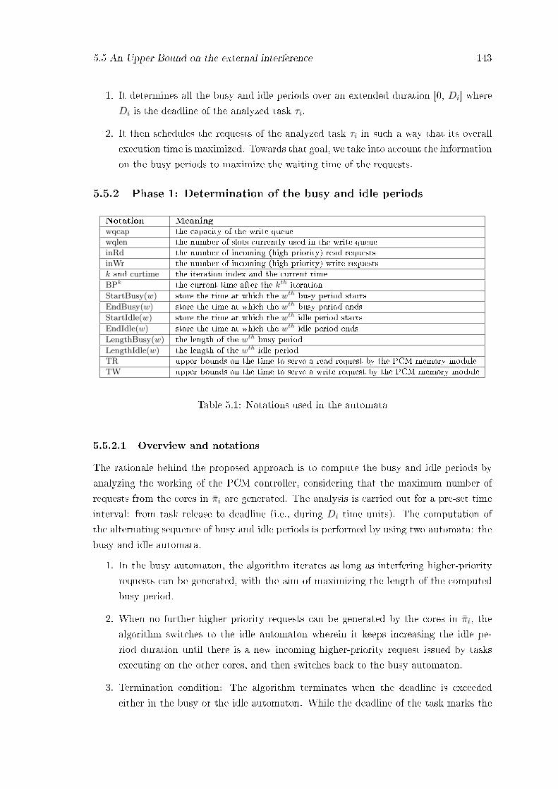
5.5 An Upper Bound on the external interference 143
1. It determines all the busy and idle periods over an extended duration [0, Di] where
Di is the deadline of the analyzed task τi.
2. It then schedules the requests of the analyzed task τi in such a way that its overall
execution time is maximized. Towards that goal, we take into account the information
on the busy periods to maximize the waiting time of the requests.
5.5.2 Phase 1: Determination of the busy and idle periods
Notation Meaning
wqcap the capacity of the write queue
wqlen the number of slots currently used in the write queue
inRd the number of incoming (high priority) read requests
inWr the number of incoming (high priority) write requests
k and curtime the iteration index and the current time
BPk the current time after the kth iteration
StartBusy(w) store the time at which the wth busy period starts
EndBusy(w) store the time at which the wth busy period ends
StartIdle(w) store the time at which the wth idle period starts
EndIdle(w) store the time at which the wth idle period ends
LengthBusy(w) the length of the wth busy period
LengthIdle(w) the length of the wth idle period
TR upper bounds on the time to serve a read request by the PCM memory module
TW upper bounds on the time to serve a write request by the PCM memory module
Table 5.1: Notations used in the automata
5.5.2.1 Overview and notations
The rationale behind the proposed approach is to compute the busy and idle periods by
analyzing the working of the PCM controller, considering that the maximum number of
requests from the cores in π̄i are generated. The analysis is carried out for a pre-set time
interval: from task release to deadline (i.e., during Di time units). The computation of
the alternating sequence of busy and idle periods is performed by using two automata: the
busy and idle automata.
1. In the busy automaton, the algorithm iterates as long as interfering higher-priority
requests can be generated, with the aim of maximizing the length of the computed
busy period.
2. When no further higher priority requests can be generated by the cores in π̄i, the
algorithm switches to the idle automaton wherein it keeps increasing the idle pe-
riod duration until there is a new incoming higher-priority request issued by tasks
executing on the other cores, and then switches back to the busy automaton.
3. Termination condition: The algorithm terminates when the deadline is exceeded
either in the busy or the idle automaton. While the deadline of the task marks the

144 Bus Contention Analysis of Phase Change Memory based Multicores
end of the analysis interval in the proposed approach, other parameters like a speci�c
threshold on the number of busy periods may be used to limit this interval.
Before modeling the working of the PCM controller to capture the worst-case scenario
(in terms of sequence of busy and idle periods), a pre-requisite is to capture the maximum
number of requests that can be issued from the interfering cores (i.e., the cores in π̄i) in any
given time interval. We leverage the function PCRPp(t) de�ned in Chapter 3 to compute
the required interference from tasks of higher priority and compute the lengths of the busy
and idle periods. The notations used are shown in Table 5.1.
Since the function PCRPq(t) did not di�erentiate between read and write requests,
we introduce two new functions: PCRPRq(i, t) and PCRPWq(i, t) that denote an upper
bound on the number of reads and write requests of higher priority (than the requests of
task τi) generated by core πq in a time interval of length t. Then, for the analyzed task τiwe denote by NHR(i, t) (NHW(i, t), resp.) an upper bound on the cumulative number of
read (write, resp.) requests issued from tasks in hp(i) executing on the other cores (in π̄i)
in a time interval of length t.
NHR(i, t) =∑q∈π̄i
PCRPRq(i, t) (5.3)
NHW(i, t) =∑q∈π̄i
PCRPWq(i, t) (5.4)
For brevity, we will drop the task index i in the automata and denote the functions as
NHR(t) and NHW(t).
k=0, BPk = curtime = TW , wqlen = wqcap
inRd = NHR(BPk) , w = 0 inWr = NHW(BPk), StartBusy(w) = 0
wqlen + inWr < wqcap?
BPk+1 = (BPk) + inRd*TR
wqlen += inWr
Yes ( The write queue is not full)
No (write queue is full)
Store the writes in the write queues and service high priority reads
inWr = inWr – (wqcap – wqlen) + 1 BPk+1 = BPk + inRd*TR + inWr * TW
wqlen=wqcap-1
inRd = NHR(BPk+1 ) - NHR(BPk ) inWr = NHW(BPk+1 ) - NHW(BPk )
ε inRd > 0 or
inWr > 0 ? Yes
k++
No
curtime = curtime + BPk+1 EndBusy(w)=curtime
LengthBusy(w) = BPk+1 - BP0
Compute new incoming requests
Any incoming requests ?
Service high priority reads and writes
Move to the wth idle period
From the idle period (Get inRd and inWr)
k=0, BPk=curtime
StartBusy(w) = curtime
Start here
Send curtime
Init variables
Figure 5.2: The busy period automata

5.5 An Upper Bound on the external interference 145
5.5.2.2 The busy period automaton
The �owchart in Figure 5.2 models the working of the PCM controller when read and/or
write requests are generated by the higher priority tasks running on the cores in π̄i. Note
that the termination condition is not shown explicitly, but whenever the variable curtime
exceeds the deadline, the automation is exited.
To create the scenario leading to the maximum duration of the busy period, the algo-
rithm begins with the initial condition that the write queue is full, re�ected by wqlen =
wqcap, and that a write request is currently being served (hence BP0 = TW). Before each
iteration in the main loop, the algorithm checks if there is any new incoming read or write
requests from the higher priority tasks. The incoming write requests may cause the write
queue to over�ow.
The PCM controller decides which request to schedule based on the current write queue
occupancy. Note that the status of the write queue (Full or Non-Full) is decided taking
into account the current occupancy of the write queue and the number of incoming write
requests. Two cases may arise:
Case 1. If the write queue is not full, the algorithm takes the right branch of the �owchart.
Since the incoming writes can be bu�ered in the queue (re�ected by �wqlen+=inWr�), the
controller serves only the read requests. The delay inRd × TR is thus added to the total
busy period length.
Case 2. If the write queue is or will be full, at least one new incoming write request
cannot be bu�ered and the cores issuing them are stalled (the algorithm takes the left
branch). The controller then starts serving read and write requests in priority order until
the write queue is non-full again (in other words, the controller does not have to serve all
the pending write requests). In the worst-case scenario, it has to serve all the pending read
requests plus enough write requests (including new incoming requests) so that the write
queue is no longer full.
Example 3. Assume that the capacity of the write queue is 6, 4 slots are currently occupied
and there are 2 incoming read requests and 5 incoming write requests. In the worst case,
the controller has to serve the 2 incoming reads but only inWr − (wqcap − wqlen) + 1 =
(5− (6− 4) + 1) = 4 writes, after which 5 slots will be occupied in the write queue and thus
there will be one vacant slot (i.e., the queue is non-full again).
The variables wqlen and inWr are correspondingly updated to re�ect the execution of
this procedure and the delay (inRd×TR +inWr×TW), computed with the reduced value
of inWr, is added to the total busy period length. When there are no more read nor write
requests issued between BPk and BPk+1 from higher priority tasks in hp(i) running on
cores in π̄i, the process terminates and the controller is free to serve requests of other lower
priority tasks (including those of τi). The length of the current (i.e., the wth) busy period
is given by LengthBusy(w) = BPk−BP0. The variable curtime is updated by a delay of
LengthBusy(w) and the algorithm moves to the idle automaton.
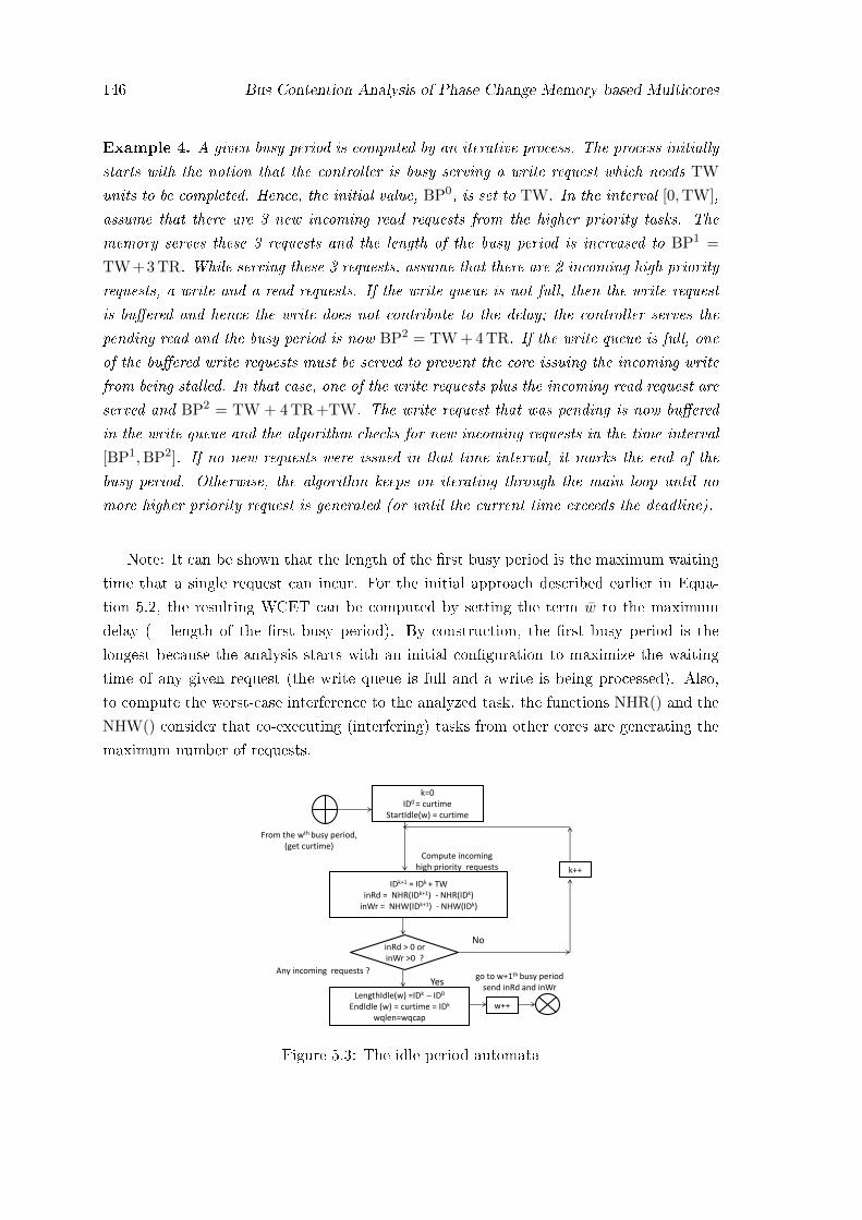
146 Bus Contention Analysis of Phase Change Memory based Multicores
Example 4. A given busy period is computed by an iterative process. The process initially
starts with the notion that the controller is busy serving a write request which needs TW
units to be completed. Hence, the initial value, BP0, is set to TW. In the interval [0,TW],
assume that there are 3 new incoming read requests from the higher priority tasks. The
memory serves these 3 requests and the length of the busy period is increased to BP1 =
TW+3 TR. While serving these 3 requests, assume that there are 2 incoming high priority
requests, a write and a read requests. If the write queue is not full, then the write request
is bu�ered and hence the write does not contribute to the delay; the controller serves the
pending read and the busy period is now BP2 = TW + 4 TR. If the write queue is full, one
of the bu�ered write requests must be served to prevent the core issuing the incoming write
from being stalled. In that case, one of the write requests plus the incoming read request are
served and BP2 = TW + 4 TR +TW. The write request that was pending is now bu�ered
in the write queue and the algorithm checks for new incoming requests in the time interval
[BP1,BP2]. If no new requests were issued in that time interval, it marks the end of the
busy period. Otherwise, the algorithm keeps on iterating through the main loop until no
more higher priority request is generated (or until the current time exceeds the deadline).
Note: It can be shown that the length of the �rst busy period is the maximum waiting
time that a single request can incur. For the initial approach described earlier in Equa-
tion 5.2, the resulting WCET can be computed by setting the term w̄ to the maximum
delay (= length of the �rst busy period). By construction, the �rst busy period is the
longest because the analysis starts with an initial con�guration to maximize the waiting
time of any given request (the write queue is full and a write is being processed). Also,
to compute the worst-case interference to the analyzed task, the functions NHR() and the
NHW() consider that co-executing (interfering) tasks from other cores are generating the
maximum number of requests.
k=0 ID0 = curtime
StartIdle(w) = curtime
IDk+1 = IDk + TW inRd = NHR(IDk+1) - NHR(IDk)
inWr = NHW(IDk+1) - NHW(IDk)
>>>ε
inRd > 0 or inWr >0 ?
Yes
No
k++
Any incoming requests ?
w++
go to w+1th busy period
send inRd and inWr
Compute incoming high priority requests
LengthIdle(w) =IDk – ID0 EndIdle (w) = curtime = IDk
wqlen=wqcap
From the wth busy period, (get curtime)
Figure 5.3: The idle period automata

5.5 An Upper Bound on the external interference 147
5.5.2.3 The idle period Automaton
The idle period marks the phase in which there are no new requests from the higher priority
tasks in hp(i) running on the cores in π̄i. The requests generated by the analyzed task τi,
if issued, may be served by the memory controller. Note that requests from low-priority
tasks can also be serviced, but the algorithm we are describing is considering only requests
from τi. Figure 5.3 depicts the �ow through the automation. Note that the termination
condition is not shown explicitly, but whenever the variable IDk exceeds the deadline, the
automation is exited.
The algorithm determines the length of the idle period by starting from the end of
the last busy period; this time-instant is recorded in curtime. The iteration index k is
initialized to 0 and ID0 is set to curtime. The central idea of identifying an idle period is
to poll at regular time instants if there are new requests being issued by the higher priority
tasks. If there are no new requests, then the algorithm increases the idle period duration
by the poll interval and continues looping in the idle automaton. If there are new incoming
requests, the algorithm switches back to the busy automaton. Note that at the beginning,
we assume that a write request was issued by a lower priority task in order to initiate the
loop.
An important design issue is determining the ideal poll interval. A very small poll
interval will allow us to capture the idle periods in small steps, leading to a longer analysis
time if there are no higher priority requests issued during a long time, whereas a large
poll interval will capture the arrival of new requests faster, but as a consequence overlooks
(precious) idle gaps between two distant polling points. We assume a polling step of TW
in the analysis, (assuming a hypothetical write request to be issued) as seen in Figure 5.3.
There can be two cases depending on the arrival of requests between two polling in-
stants.
1. No new requests are issued: The algorithm increases the length of the idle period
(IDk+1 = IDk + TW) and proceeds to the next iteration.
2. New requests are issued: This marks the end of the idle period. The algorithm up-
dates the current time to IDk, computes the duration of the idle period and switches
back to the busy period automaton.
5.5.3 Phase 2: Using the pre-computed busy and idle periods of the
analyzed task to compute its increased WCET
5.5.3.1 Modeling Sampling Regions
This section focuses on computing a tight upper-bound for the cumulative waiting times
of all the requests generated by a given task τi by considering the busy periods computed
in Phase 1. The waiting time for a given request is maximized if it is issued just before

148 Bus Contention Analysis of Phase Change Memory based Multicores
the longest (feasible) busy period (the request is issued but the bus has just started serv-
ing a contiguous stream of requests of higher priority). The cumulative waiting time is
maximized by adding up the maximum waiting times of each requests (delays incurred due
to the busy periods) which in turn results in an upper bound of the worst-case execution
time of τi. To compute the increase in WCET, we start by modeling the memory request
pro�le of the analyzed task τi in isolation. The memory pro�ling is done by dividing τiinto logical sampling regions and determining the maximum number of requests issued in
each of these regions. The number of memory requests generated in each region can be
determined by static cache analysis [10] or by measurements by instrumenting the L2 cache
misses [79] (using performance monitoring counters [94]).
For this analysis, we assume that the analyzed task τi is sampled in intervals of length
lenregion and has NSRi such sampling regions. That is, the worst-case execution time Ciof τi is split into NSRi regions, each of length lenregion: NSRi × lenregion = Ci. We can
also generalize it to di�erent regions of unequal length lenregionj where {j ∈ 1 . . .NSRi},
but will keep it simple at this stage. We denote by N readi,j and Nwrite
i,j the maximum number
of read and write requests (respectively) that can be generated in the jth sampling region
of task τi denoted by SRi,j , where 1 ≤ j ≤ NSRi.
5.5.3.2 Description of Algorithm CompConDelay()
During the sampling of τi, the WCET of each region is determined by considering a �nite
service time of TR time units for the read request but a zero waiting time for the write
requests. That is, the memory traces obtained at design time assume that the write queue
is never full and all the write requests are thus bu�ered in the queue as soon as they are
generated. This implies that the time for servicing every read request is accounted for in
the original WCET Ci (and thus in the per-region WCET (lenregion) as well), whereas
the time for servicing the write requests must be taken into consideration in the analysis.
To this end, line 2 of Algorithm 7 adds the following to lenregion:
1. Nwritei,j ×TW, since the time for servicing write requests is not factored in the original
WCET.
2. (Nwritei,j +N read
i,j )× TW, because every request of τi may be generated just after the
PCM controller starts serving a lower-priority write request. Since the PCM serves
requests in a non-preemptive manner, every request of τi can potentially be subjected
to an extra delay of TW time units.
For each sampling region of τi, lines 4 and 5 compute the interval of time [tstartj , tend
j ] during
which the jth region executes (in the worst-case scenario): the jth region starts after the
(j − 1)th region completes (assuming tend0 = 0) and ends wceti,j time units later. During
this time interval, each request of τi will be assigned the maximum possible delay. The
requests of a given region are considered in sequence (line 7).
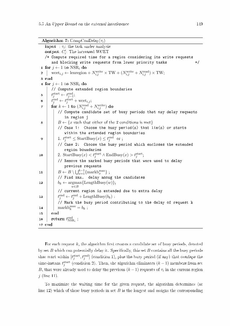
5.5 An Upper Bound on the external interference 149
Algorithm 7: CompConDelay(τi)input : τi: the task under analysisoutput: C ′i: The increased WCET/* Compute required time for a region considering its write requests
and blocking write requests from lower priority tasks */
1 for j ← 1 to NSRi do2 wceti,j ← lenregion +Nwrite
i,j × TW + (Nwritei,j +N read
i,j )× TW;3 end4 for j ← 1 to NSRi do
// Compute extended region boundaries
5 tstartj ← tend
j−1;6 tend
j ← tstartj + wceti,j ;
7 for k ← 1 to (N readi,j +Nwrite
i,j ) do
// Compute candidate set of busy periods that may delay requests
in region j
8 B ← {x such that either of the 2 conditions is met}// Case 1: Choose the busy period(s) that lie(s) or starts
within the extended region boundaries
9 1. tstartj ≤ StartBusy(x) ≤ tend
j or ;// Case 2: Choose the busy period which encloses the extended
region boundaries
10 2. StartBusy(x) < tstartj ∧ EndBusy(x) > tstart
j ;// Remove the marked busy periods that were used to delay
previous requests
11 B ← B \⋃k−1x=1{markbmax
x } ;// Find max. delay among the candidates
12 bk ← argmaxw∈B
{LengthBusy(w)};
// current region is extended due to extra delay
13 tendj ← tend
j + LengthBusy(bk) ;// Mark the busy period contributing to the delay of request k
14 markbmaxk = bk ;
15 end
16 return tendNSRi
;17 end
For each request k, the algorithm �rst creates a candidate set of busy periods, denoted
by set B which can potentially delay it. Speci�cally, this set B contains all the busy periods
that start within [tstartj , tend
j ] (condition 1), plus the busy period (if any) that overlaps the
time-instant tstartj (condition 2). Then, the algorithm eliminates (k− 1) members from set
B, that were already used to delay the previous (k− 1) requests of τi in the current region
j (line 11).
To maximize the waiting time for the given request, the algorithm determines (at
line 12) which of these busy periods in set B is the longest and assigns the corresponding

150 Bus Contention Analysis of Phase Change Memory based Multicores
Busy period
Idle period
time lenb1
lenb1
lenb2
lenb2
Figure 5.4: Visualization of the variables used in Algorithm 7. The task index is droppedin the wcet notation and only the region index j is retained
delay (assumed to be zero if B is empty) to the current request k. As the request is delayed,
the length of the region is extended, which is re�ected by the increase of tendj at line 13.
Finally, the increased WCET C ′i of τi corresponds to the end of last region, NSRi and is
captured in the variable tendNSRi
, which is returned at the end of the entire analysis.
Note that the increased WCET (C ′i) being less than the deadline Di does not auto-
matically imply that τi is schedulable (i.e., will meet its deadline when scheduled with
other tasks). All the tasks parameters (including their increased WCET) have to be fur-
ther provided as an input into a schedulability analysis tool, which will assess the system
schedulability by also considering the on-core interference. The focus of this work is to
compute the increased WCET; the schedulability analysis should be carried out using
existing approaches.
5.5.4 Proof of safety of Algorithm CompConDelay()
Next we provide a proof that our method indeed computes an upper bound, as desired, on
the execution time of a task including the delays due to accesses to PCM.
Lemma 7. The value of C ′i returned by Algorithm 7 is a safe upper-bound on the execution
time of τi, considering the contention on the shared memory.
Proof. The proof is obtained step-by-step, by examining the properties of all the time-
instants tendj computed by the algorithm. Recall that j indexes the region being examined
and k is used to index the request.
For the �rst region (j = 1), the value of tend1 computed at line 6 is an upper-bound on
the completion time of the �rst region of τi, assuming that none of the requests generated
by this region is blocked by higher-priority requests (see Figure 5.4). When j = 1 and
k = 1, it can be seen that the value of tend1 (re-computed at line 13) is an upper-bound on
the completion time of this �rst request since it considers the maximum blocking for that
request. Therefore, during the second iteration in the inner loop (i.e., when k = 2), the

5.5 An Upper Bound on the external interference 151
set B computed at line 8 is guaranteed to contain the maximum number of busy periods
that can potentially be used to block a second request. This implies in turn that the
value of tend1 computed for the third time at line 13 (during this second iteration when
k = 2) is an upper-bound on the completion time of the �rst region, assuming that two
requests are blocked by higher-priority requests. The same reasoning can be applied for
every subsequent request until the (N read1 +Nwrite
1 )th request and thus, tend1 is guaranteed
to eventually provide an upper-bound on the completion time of the �rst region when all
its requests can be blocked by higher-priority requests.
Note that during the last iteration (when j = 1 and k = N read1 + Nwrite
1 ), tend1 is
increased for the last time at line 13. Let tend1,last−1 and tend
1,last denote the values of tend1
before and after this last increase. To visualize this, let us assume in Figure 5.4 that the
�rst region can generate only two requests. By construction of the algorithm, none of the
busy periods starting within [tend1,last−1, t
end1,last] can be used to block any request generated in
this �rst region (since there are no more requests from the �rst region to block). Among
those busy periods, some may have their starting and ending times within this interval
[tend1,last−1, t
end1,last] while at most one busy period may start within [tend
1,last−1, tend1,last] and end
after tend1,last. Let us denote by BPlast this last busy period that overlaps tend
1,last.
Regarding the busy periods that start and end within [tend1,last−1, t
end1,last], it is not inter-
esting (in order to maximize the WCET) to assume that the �rst region �nishes earlier
than their starting times (i.e., at time tend1,last−1) so that requests from the second region
can �use� these busy periods to increase the overall delay. Assuming so would imply that:
1. after tend1,last time units of execution, τi is already progressing in its second region (while
it could still be executing its �rst region without this assumption) and,
2. it uses some requests from the second region to take advantage of these busy periods
(and these requests could be used later to further increase the overall delay).
However, in order to maximize the cumulative delay, it might be interesting to consider
the busy period BPlast to block a request of the second region (this will be taken care
of during the next iteration of the outer loop). To explore the second region, when j=2
(Line 4), the algorithm �rst computes the interval of time [tend1 , tend
1 + wcet2], where the
value of tend2 is an upper-bound on the completion time of the second region, assuming that
all the requests of the �rst region have incurred the maximum possible delay but none of
the requests of the second region have been blocked by higher-priority requests. Then, the
set B is computed (Line 8) and it can be seen that the busy period BPlast is included in
that set, thanks to the second condition. By using the same reasoning as above, we can
infer that after the (N read2 + Nwrite
2 )th iteration in the inner loop (lines 7�16), tend2 is an
upper-bound on the completion time of the second region of τi. Following this reasoning,
we can see that ultimately tendNSRi
is an upper-bound on the execution time of τi. �
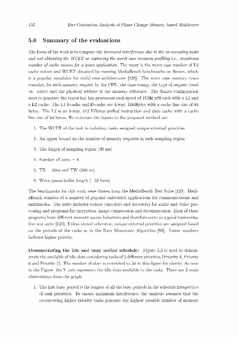
152 Bus Contention Analysis of Phase Change Memory based Multicores
5.6 Summary of the evaluations
The focus of the work is to compute the increased interference due to the co-executing tasks
and not obtaining the WCET or capturing the worst case memory pro�ling i.e., maximum
number of cache misses for a given application. The input is the worst case number of L2
cache misses and WCET obtained by running MediaBench benchmarks on Simics, which
is a popular simulator for multi-core architectures [130]. The worst-case memory trace
contains, for each memory request by the CPU, the time stamp, the type of request (read
vs. write) and the physical address of the memory reference. The Simics con�guration
used to generate the traces has has processors each speed of 1GHz x86 each with a L1 and
a L2 cache. The L1 I-cache and D-cache are 4-way, 16KBytes with a cache line size of 64
bytes. The L2 is an 8-way, 512 KBytes uni�ed instruction and data cache with a cache
line size of 64 bytes. To re-iterate the inputs to the proposed method are
1. The WCET of the task in isolation, tasks assigned unique external priorities
2. An upper bound on the number of memory requests in each sampling region
3. The length of sampling region (20 ms)
4. Number of cores = 4
5. TR = 50ns and TW (500 ns)
6. Write queue bu�er length (=32 here).
The benchmarks for this work were chosen from the MediaBench Test Suite [123]. Medi-
aBench consists of a number of popular embedded applications for communications and
multimedia. The suite includes codecs (encoders and decoders) for audio and video pro-
cessing and programs for encryption, image compression and decompression. Each of these
programs have di�erent memory access behaviors and therefore serve as a good representa-
tive test suite [131]. Unless stated otherwise, unique external priorities are assigned based
on the periods of the tasks as in the Rate Monotonic Algorithm [99]. Lower numbers
indicate higher priority.
Demonstrating the idle and busy period schedule: Figure 5.5 is used to demon-
strate the available of idle slots considering tasks of 3 di�erent priorities (Priority 4, Priority
6 and Priority 7). The number of slots is restricted to 50 in this �gure for clarity. As seen
in the Figure, the Y axis represents the idle slots available to the tasks. There are 2 main
observations from the graph.
1. The �rst busy period is the longest of all the busy periods in the schedule irrespective
of task priorities. To ensure maximum interference, the analysis assumes that the
co-executing higher priority tasks generate the highest possible number of memory
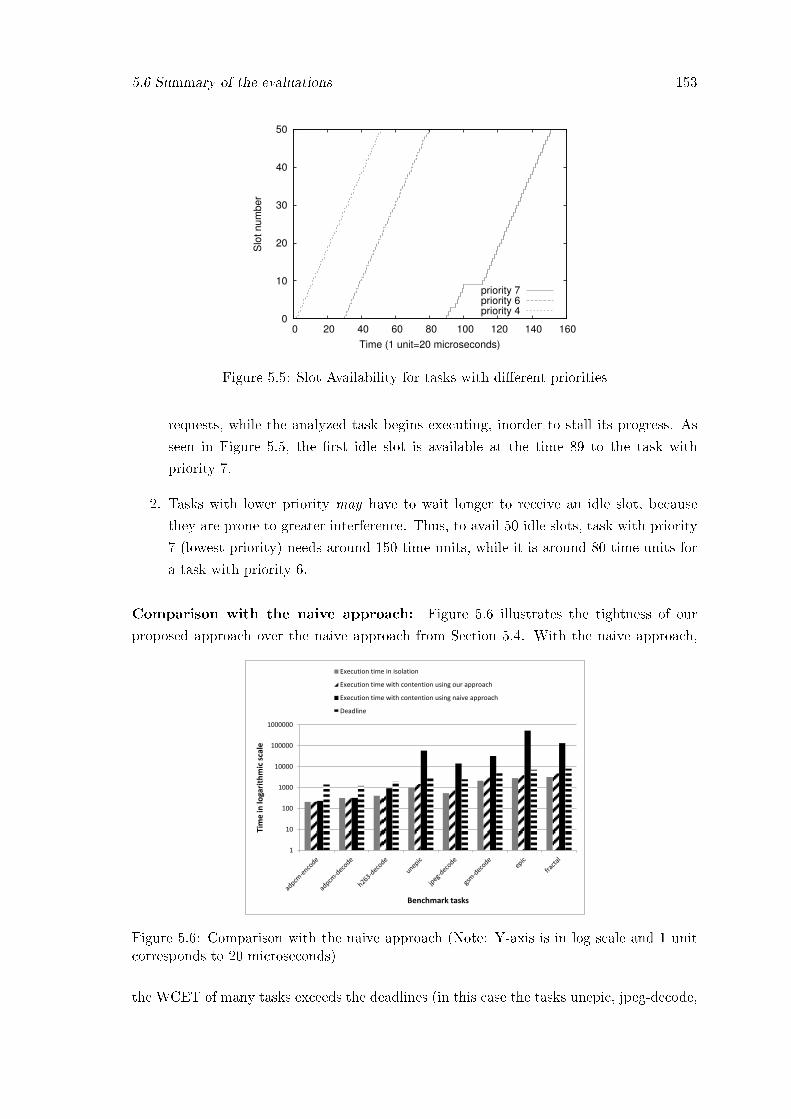
5.6 Summary of the evaluations 153
0
10
20
30
40
50
0 20 40 60 80 100 120 140 160
Slo
t n
um
be
r
Time (1 unit=20 microseconds)
priority 7priority 6priority 4
Figure 5.5: Slot Availability for tasks with di�erent priorities
requests, while the analyzed task begins executing, inorder to stall its progress. As
seen in Figure 5.5, the �rst idle slot is available at the time 89 to the task with
priority 7.
2. Tasks with lower priority may have to wait longer to receive an idle slot, because
they are prone to greater interference. Thus, to avail 50 idle slots, task with priority
7 (lowest priority) needs around 150 time units, while it is around 80 time units for
a task with priority 6.
Comparison with the naive approach: Figure 5.6 illustrates the tightness of our
proposed approach over the naive approach from Section 5.4. With the naive approach,
1
10
100
1000
10000
100000
1000000
Tim
e in
loga
rith
mic
sca
le
Benchmark tasks
Execution time in isolation
Execution time with contention using our approach
Execution time with contention using naive approach
Deadline
Figure 5.6: Comparison with the naive approach (Note: Y-axis is in log scale and 1 unitcorresponds to 20 microseconds)
the WCET of many tasks exceeds the deadlines (in this case the tasks unepic, jpeg-decode,
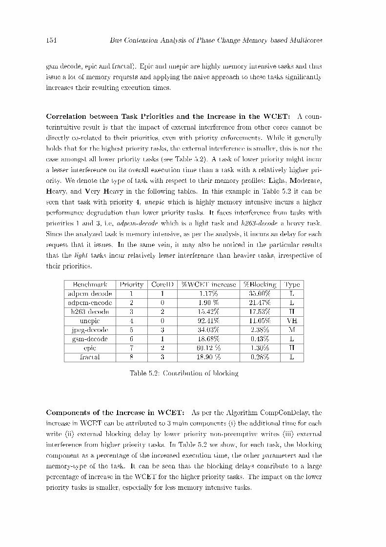
154 Bus Contention Analysis of Phase Change Memory based Multicores
gsm decode, epic and fractal). Epic and unepic are highly memory intensive tasks and thus
issue a lot of memory requests and applying the naive approach to these tasks signi�cantly
increases their resulting execution times.
Correlation between Task Priorities and the Increase in the WCET: A coun-
terintuitive result is that the impact of external interference from other cores cannot be
directly co-related to their priorities, even with priority enforcements. While it generally
holds that for the highest priority tasks, the external interference is smaller, this is not the
case amongst all lower priority tasks (see Table 5.2). A task of lower priority might incur
a lesser interference on its overall execution time than a task with a relatively higher pri-
ority. We denote the type of task with respect to their memory pro�les: Light, Moderate,
Heavy, and Very Heavy in the following tables. In this example in Table 5.2 it can be
seen that task with priority 4, unepic which is highly memory intensive incurs a higher
performance degradation than lower priority tasks. It faces interference from tasks with
priorities 1 and 3, i.e, adpcm-decode which is a light task and h263-decode a heavy task.
Since the analyzed task is memory intensive, as per the analysis, it incurs an delay for each
request that it issues. In the same vein, it may also be noticed in the particular results
that the light tasks incur relatively lesser interference than heavier tasks, irrespective of
their priorities.
Benchmark Priority CoreID %WCET increase %Blocking Typeadpcm-decode 1 1 1.17% 35.00% Ladpcm-encode 2 0 1.90 % 21.47% Lh263-decode 3 2 15.42% 17.53% H
unepic 4 0 92.41% 11.05% VHjpeg-decode 5 3 34.03% 2.38% Mgsm-decode 6 1 18.68% 0.43% L
epic 7 2 60.12 % 1.30% Hfractal 8 3 18.90 % 0.28% L
Table 5.2: Contribution of blocking
Components of the Increase in WCET: As per the Algorithm CompConDelay, the
increase in WCET can be attributed to 3 main components (i) the additional time for each
write (ii) external blocking delay by lower priority non-preemptive writes (iii) external
interference from higher priority tasks. In Table 5.2 we show, for each task, the blocking
component as a percentage of the increased execution time, the other parameters and the
memory-type of the task. It can be seen that the blocking delays contribute to a large
percentage of increase in the WCET for the higher priority tasks. The impact on the lower
priority tasks is smaller, especially for less memory intensive tasks.
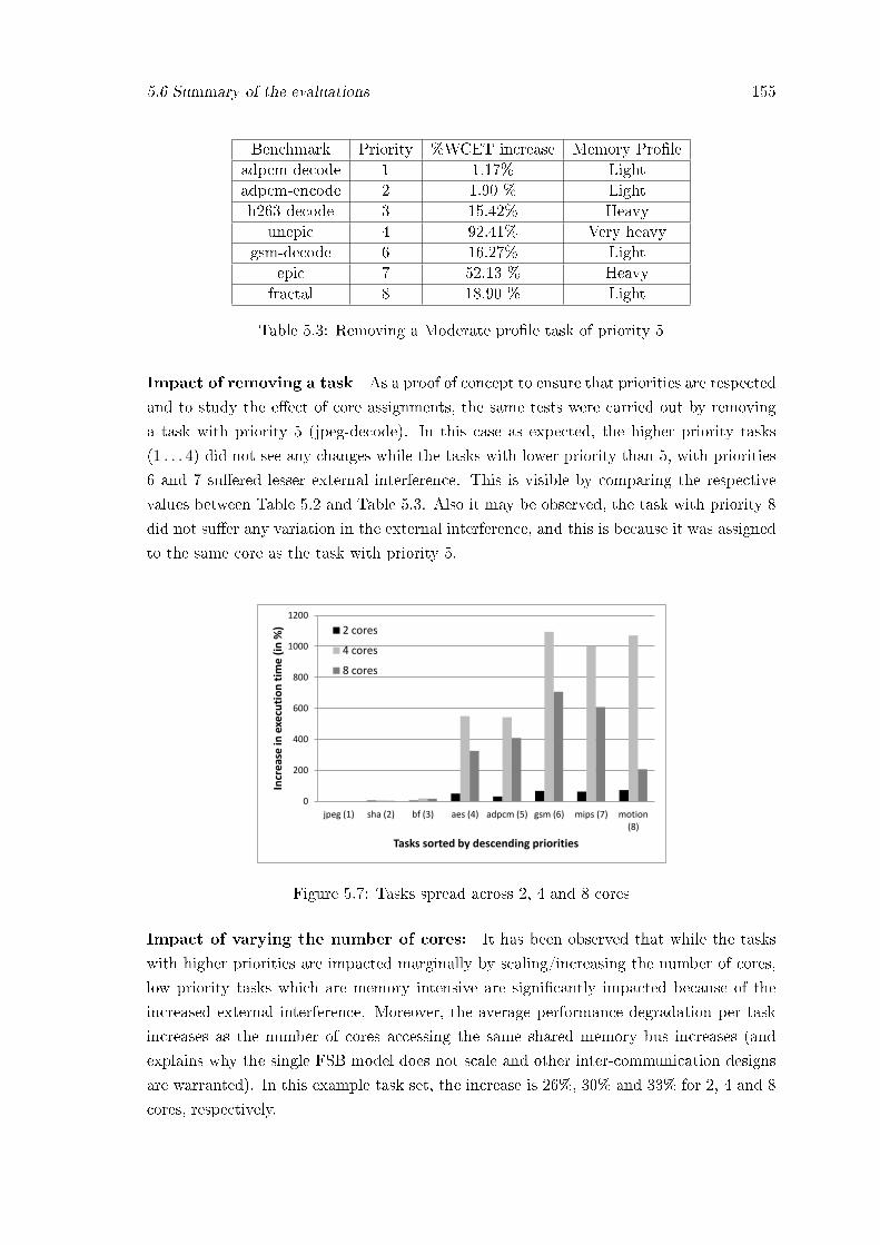
5.6 Summary of the evaluations 155
Benchmark Priority %WCET increase Memory Pro�leadpcm-decode 1 1.17% Lightadpcm-encode 2 1.90 % Lighth263-decode 3 15.42% Heavy
unepic 4 92.41% Very heavygsm-decode 6 16.27% Light
epic 7 52.13 % Heavyfractal 8 18.90 % Light
Table 5.3: Removing a Moderate pro�le task of priority 5
Impact of removing a task As a proof of concept to ensure that priorities are respected
and to study the e�ect of core assignments, the same tests were carried out by removing
a task with priority 5 (jpeg-decode). In this case as expected, the higher priority tasks
(1 . . . 4) did not see any changes while the tasks with lower priority than 5, with priorities
6 and 7 su�ered lesser external interference. This is visible by comparing the respective
values between Table 5.2 and Table 5.3. Also it may be observed, the task with priority 8
did not su�er any variation in the external interference, and this is because it was assigned
to the same core as the task with priority 5.
0
200
400
600
800
1000
1200
jpeg (1) sha (2) bf (3) aes (4) adpcm (5) gsm (6) mips (7) motion (8)
Incr
ease
in e
xecu
tio
n t
ime
(in
%)
Tasks sorted by descending priorities
2 cores
4 cores
8 cores
Figure 5.7: Tasks spread across 2, 4 and 8 cores
Impact of varying the number of cores: It has been observed that while the tasks
with higher priorities are impacted marginally by scaling/increasing the number of cores,
low priority tasks which are memory intensive are signi�cantly impacted because of the
increased external interference. Moreover, the average performance degradation per task
increases as the number of cores accessing the same shared memory bus increases (and
explains why the single FSB model does not scale and other inter-communication designs
are warranted). In this example task set, the increase is 26%, 30% and 33% for 2, 4 and 8
cores, respectively.

156 Bus Contention Analysis of Phase Change Memory based Multicores
1. Impact of task mix: As a proof of concept to ensure that priorities are respected and
to study the e�ect of core assignments, the analysis with a reference task set was
carried out by removing a task with a medium level priority. As expected, the higher
priority tasks did not see any changes while the tasks with lower priority su�ered less
external interference.
2. Impact of task assignments based on request densities: To improve responsiveness, a
possible intuitive scheduling algorithm is to prioritize tasks based on their memory
request densities (more requests, higher priority, so that they �nish earlier). With this
set of experiments, we demonstrated that this strategy will lead to the performance
degradation for most of the tasks. The e�ect is worse when highly memory intensive
tasks with higher priorities arrive more frequently.
Our experiments show that the increase in execution time for tasks is a complex function
of the task pro�les (memory or computation intensive), the task assignments to cores, the
priority enforcement mechanisms, and the temporal characteristics (the execution time and
the period of tasks).
5.7 Chapter Summary
In this chapter, we delved deeper into the memory controller and modelled its scheduling.
To ensure safe upper bounds, the impact of shared low-level resources on the timing be-
havior of tasks deployed on multicores must be taken into account while carrying out the
timing analysis. In this chapter, we presented a method to compute the increase in the
worst-case execution time of a task considering the contention on the shared Phase Change
Memory. Our proposed method takes into consideration the di�erent read and write la-
tencies of the PCM controller, the priorities of the tasks, the request scheduling of the
controller, and the interference arising from the co-executing tasks. Based on the request
scheduling policy, the proposed method �rst determines the available slots in which the
analyzed task can send its requests. The requests of the analyzed task are then assigned
to the available slots such that its worst-case execution time is maximized. Our results
using embedded benchmarks shows that there is a modest (for most real-time systems)
increase in the worst-case computation time of a task, in comparison when the task is run
in isolation; surprisingly, we noticed that the lower priority tasks do not always have a
higher increase in execution time. Comparisons against a basic approach shows that the
proposed method provides tighter upper bounds.
Chapter 6
NoC Contention Analysis of Many
Core Systems
For over a decade prophets have voiced the
contention that the organization of a single
computer has reached its limits and that truly
signi�cant advances can be made only by
interconnection of a multiplicity of computers.
Gene Amdahl in 1967
6.1 Introduction to many-core systems
The current trend in the chip manufacturing industry is towards the integration of previ-
ously isolated functionalities into a single-chip. Following this trend, the usage of multi-
cores has become ubiquitous, not only for general-purpose systems but also in the em-
bedded computing segment. Besides the increasing processing demand, advancements in
the semiconductor arena have fostered in the �many-core� systems era and we are now
witnessing the emergence of chips enclosing upto hundreds of cores. With the increase in
the number of cores, the currently popular bus structure implementation prevents e�cient
scalability beyond eight cores in multicore processors where every memory request has
to go through a central arbitration unit creating a critical bottleneck. To overcome this
limitation, many-core designers developed a mesh-based tile architecture in which each
building block called a tile consists of a processing core, a private cache plus a switch.
This technology eliminates the single bus (bottleneck) by placing a communications switch
on each processor core and arranging them in a grid fashion on the chip. This creates an
e�cient 2-dimensional tra�c system for packets. Each tile in the grid is connected to its
(up to 4) neighboring tiles located in the cardinal directions, thereby forming a 2D-mesh
(c.f. right plot of Figure 6.1). The NoC serves as a communication channel among the cores
157

158 NoC Contention Analysis of Many Core Systems
and between the cores and other o�-chip subsystems, e.g. the main memory. Such many-
core systems o�er evident enhanced computational capabilities compared to the former
(traditional) multi-core platforms. The Tile-Gx72 with 72 cores from Tilera [21], Kalray
with 256 cores [22], Epiphany with 64 cores from Adapteva, Intel Xeon co-processor [23]
with 60 cores and the 48-core Single-Chip-Cloud computer [24] are just some examples
of many-core architectures. These systems like Kalray's MPPA (Multi-Purpose Processor
Array) have been optimized to address the demand of high performance, low power em-
bedded systems and are therefore these architectures must be analyzed. In this document
we focus on the structure and terminology of the Tile64 platform, but our analysis extends
to other platforms which �ts the assumed system model.
Core1 Core2 Core3
Memory controller
Front-Side-Bus
Core4 Tile1 Tile2
Tile3
Memory controller
Tile4
Core3
switchNoC
cache
Traditional multicores architecture Massive multicores architecture
Figure 6.1: Multi-core vs. many-core systems
6.1.1 Motivation: Real-time applications and many-core systems
Although many-core systems o�er various opportunities in terms of performance and com-
puting capabilities, they do pose many challenges for the deployment of real-time systems,
which must ful�ll speci�c timing requirements at run time � It is therefore essential to
identify, at design time, the parameters that have an impact on the execution time of the
tasks deployed on these systems and the upper bounds on the other key parameters. It is
also vital to derive an upper bound on the execution time of these applications at design
time itself before these applications can be deployed � but this is non-trivial, for the
reasons stated below.
In a scenario involving data transfers (amongst cores or from cores to memory), the
execution time of a task running on a given core increases as the core stalls waiting for
the data to be transferred over the underlying network. This waiting time can lead to
a substantial increase in the execution time when the tra�c on the network and thus

6.2 Related Work 159
the contention for the network resources increases. Additionally, depending on their re-
spective behavior, tasks running on di�erent cores may release packets over the network
independently and asynchronously. All the packets are transmitted over the same underly-
ing interconnection network and share the available network resources like links and �nite
sized bu�ers (which prohibit the constant in�ux of packets after reaching a given limit).
Thus the time to transmit a packet depends on the current load of the network, which
is in turn determined by the number of packets generated by the tasks executing on the
other cores. Other factors like the routing mechanism employed also impacts the traversal
times as it in�uences the path taken by the packets to reach their destination �this in-turn
decides whether they would directly or indirectly block the analyzed packet by contending
for the same resources. The contention for the shared network thus leads to a substan-
tial increase in the resulting traversal time of the analyzed packet. Additionally, tasks on
di�erent cores can release packets at arbitrary times on the shared communication infras-
tructure and these exact release time-instants are not known beforehand. To summarize,
the number of parameters contributing to the unpredictability combined with the large
number of cores poses a challenging problem to designers aiming to determine an upper
bound on the traversal time of a (message/memory/IO) packet . In this work, we aim to
compute such an upper bound which we refer to as the worst-case traversal time (WCTT)
for a NoC based many-core system employing a wormhole switching technique [132].
The focus of this chapter is to determine an upper bound on the traversal time of a
packet when it is transmitted over the NoC infrastructure. Towards this aim, we �rst
identify and explore some limitations in the existing recursive-calculus based approaches
to compute the worst-case traversal time (WCTT) of a packet. Then, we extend the
existing model by integrating the characteristics of the tasks that generate the packets.
For this extended model, we propose an algorithm called �Branch and Prune� (BP). Our
proposed method provides safe and tighter estimates than the existing recursive-calculus
based approaches. Finally, we introduce a more general approach - �Branch, Prune and
Collapse� (BPC) which o�ers a con�gurable parameter that provides a �exible trade-o�
between the computational complexity and the tightness of the computed estimate. The
recursive-calculus methods and BP present two special cases of BPC when the trade-o�
parameter is set to 1 or ∞, respectively. Through simulations, we analyze this trade-o�,
reason about the implications of certain choices and also provide some case studies to
observe the impact of task parameters on the WCTT estimates.
6.2 Related Work
A signi�cant amount of research has been carried out on exploring the impact of the
interconnect networks in systems employing wormhole switching [133]. In the works of [134]
and [132], the respective authors elaborated on the estimation of end-to-end delays for
wormhole switching networks, but with the primary focus on the determination of the

160 NoC Contention Analysis of Many Core Systems
average latencies using queuing theory techniques. As mentioned earlier, in real-time
systems, estimation of the worst case latencies rather than average case latencies is vital.
Hence the earlier approaches do not su�ce to perform a real-time analysis.
To ensure predictability and derive an upper bounds on the communication delay, some
researchers have used mechanisms which require special hardware support to the NoC as
in [135], priority mechanisms [136], time-triggered systems [137] and time division multiple
access (TDMA) [138]. All these approaches assume that the basic NoC is designed to
support predictability, but as seen in a survey of NoCs [139], existing commercial of the
shelf (COTS) based NoC architectures are more suited to provide best e�ort service and
hence to model the existing systems, a software-based analysis is warranted.
The existing works which address the issues of the worst-case end-to-end communication
latencies in standard NoC-based many-cores can be broadly categorized into two groups:
approaches applying network calculus and approaches applying Recursive calculus (RC).
We borrowed the terminology RC from a previous approach [140].
Network Calculus (NC) based methods: In general queuing networks, network cal-
culus [141] provides an elegant way to express and deal with the timing properties of tra�c
�ows. Based on the powerful abstraction of arrival curves for tra�c �ows and service curves
for network elements like routers and servers, it facilitates the computation of the worst-
case delay and backlog bounds. For wormhole switching based networks, �ow control is
based on feedback received from the next router (downstream router). Determining the
service curve of a given router independently (without the knowledge of the service curve
of the next router involved in the transfer) is not straightforward by the basic abstractions
provided by network calculus theory (which is designed to deal with forward networks)
since there is a cyclic dependency between the service curves of the routers involved in the
transfer.
To overcome this, Qian et.al [142] have modeled the �ow control mechanism in the
switch itself as another service curve. But in another related work by Ferrandiz et. al [143]
clearly showed with an illustrative example the �aws of the design. The authors [143]
consider a space wire network topology and introduced a special network element called
the �wormhole section� to describe the wormhole routing with the network-calculus ter-
minology. This element envelopes a set of routers lying in the shared path between an
analyzed �ow and the blocking �ow(s): the analyzed and the blocking �ows enter the
�rst router and exit through the last router of the wormhole section, with no additional
blocking �ows either entering or leaving from any other link within the wormhole section.
The analysis treats this section as a single element, with the arrival and service curves
computed as a function of the individual curves of the �ows contained within the section.
Finally, an end-to-end service curve is derived by combining the service curves of all the
wormhole sections in the path of the analyzed �ow. In the presence of diverse tra�c (with
intersecting blocking �ows with short shared paths), the direct application of this method

6.2 Related Work 161
on the NoC-based many-core platform would force a wormhole section fragmentation, i.e.
every router would be treated as an individual element, which renders the purpose of the
wormhole section obsolete, and the results pessimistic.
Recursive Calculus (RC) based methods: The methods centered around this paradigm
compute the end-to-end delays by recursively analyzing the contention at each router in
the path of the analyzed �ow. As a common denominator in these approaches is the ra-
tionale that �ows inject packets at the maximum rate to saturate the network. The initial
assumption of these approaches is that all the intermediate bu�ers in the switches between
the source and the destination are �lled to their capacity [140]. The method thus ensures
capturing the worst-case scenario.
The works of Lee et. al [144], Rehmati et. al [145] and Ferrandiz et. al [146] have been
noteworthy in this area. Initially, Lee et. al [144] proposed a model for real-time commu-
nication in wormhole networks based on the use of real-time wormhole channels. This was
improved by Rehmati et. al [145] by computing real-time bounds for high bandwidth tra�c
in which they assume that all intermediate bu�ers are full, and for low latency regulated
tra�c, the concept of lumping �ows is combined with the method of Ferrandiz et.al [146].
Lu et.al [147] proposed a contention tree based approach focused on feasibility analysis for
a set of periodic messages with pre-assigned priorities, which were used to resolve arbitra-
tion con�icts in the switch. Their model does not classically fall into the recursive calculus
based methods but it introduced the concept of contention trees (to capture direct and
indirect blockings) which are analyzed in a recursive manner and thus conceptually �ts in
this category (and not in the NC based approaches).
In the approach proposed by Ferrandiz et.al [146], which is conceptually similar to the
method of Rehmati et.al [145], an upper-bound on the traversal delay is computed, but
with the assumption that the packets can be injected into the network continuously and
therefore the computed WCTT is not tight.
The key advantage of these methods is that they compute the WCTT with low time
complexity, but the main limitation is that they do not leverage the input arrival patterns
and hence lead to over-approximations of the WCTT. Hence a method which provides
tighter WCTTs in acceptable times is warranted.
Positioning our approach: In a very recent work by Ferrandiz et. al [140], the authors
compare their newly proposed NC method against their previous RC method considering
di�erent parameters. In our approach we combine the best of both methodologies - an
ability to exploit the simplicity and intuition behind RC methods without losing the in-
put tra�c characterization provided by NC methods. We �rst identify the key sources of
pessimism in RC methods and introduce methods to characterize the tra�c patterns. We
then formulate a �Branch and Prune� algorithm which leverages these input characteristics
inorder to eliminate packets which cannot arrive at run-time owing to task constraints and

162 NoC Contention Analysis of Many Core Systems
thus derive tighter bounds than the existing methods. We also propose a more general ap-
proach called �Branch, Prune and Collapse� which through a controllable parameter, o�ers
the designer a trade-o� between the tightness of the bound and computational complexity.
By performing the simulations, we validate and verify the performance of our algorithm in
comparison with the RC-based approach presented by Ferrandiz et. al [146] and observe
that our approach dominates this method by yielding at least as tight as and in most
cases tighter WCTT estimates than the related work. We investigate the in�uence of the
trade-o� parameter on the derived bounds.
The rest of the chapter is organized as follows: Section 6.3 describes the basic system
model followed by the input characterization in Section 6.4. A brief description of the
approach presented by Ferrandiz et.al [146] is described in Section 6.5. We introduce
the basis of our method in Section 6.6. We propose the Branch and Prune algorithm in
Section 6.7 followed by its variant in Section 6.8. The evaluations of the approaches are
presented in Section 6.9. We �nally summarize the work in Section 6.10.
6.3 System Model
6.3.1 Platform and Application Model
Platform model As previously noted, without loss of generality we drive our discussion
in the context of tile-based platforms from Tilera. As seen in Figure 6.2, the tile-based
architecture uses a 2D-mesh network to interconnect the processors and serves as the
transport channel for o�-chip memory access, I/O, interrupts, and other communication.
As illustrated in Figure 6.1, each tile comprises a general purpose processing engine
(core), a cross-bar switch and a private cache. The platform is thus structured as a grid
of m× n tiles, where �m� and �n� are the dimensions of the grid and r o�-chip subsystems
(e.g. memory controllers).
Another variation is the Intel SCC with the speci�cation below:
Example 5. The IA core on the SCC is based on the P54C core. The 48 cores are placed
in a tile formation with 2 cores per tile and are connected by a 6 * 4 2D mesh fabric. Each
of the P54C is a simple in-order processor having 2 level caches with on core L1 (16KB
data, 16KB instruction) and uni�ed 256KB L2. Each caches level are private to a given
core so that there is no concurrent access to the cache between cores [148].
Our model conforms to the above architecture, but by assuming a single tile per core
to simplify the discussion. The o�-chip subsystems are connected to some of the tiles on
the periphery of the grid. Inter-tile communication is achieved by routing packets via the
embedded switches. Note that the terms router and switch are used interchangeably in
the rest of the chapter.
Each tile contains a switch engine. The switch engine connects to neighboring tiles
and I/Os (including the on-chip memory controllers) via the intra-tile network. The tiles

6.3 System Model 163
DDR3 Controller
DDR3 ControllerSm
art
NIC
Con
trol
ler
NetworkI/O
Two 10 Gb
&Two1Gb
UART x2USB x2JTAG
12C, SPI
PCIe 2.08 Lanes
PCIe 2.04 Lanes
Flexible I/O
Figure 6.2: Tilera architecture. (Diagram taken from [21])
are laid out in a two dimensional grid, thus the switch engine connects to the neighbors
to the north, south, east, and west. The switch engine connects directly to I/O devices
if a tile is adjacent to an I/O device. Generally, the switch that is embedded in each tile
is part of several networks. Independent networks are typically used to handle di�erent
types of tra�c to minimize the interference and maximize the performance. For example,
the TILEProTMand TILE64TMfamily of chips employ distinct networks to transmit tra�c
related to memory, caches, I/O and inter-tile communication between applications. Since
a packet can travel (and interfere with other packets) only over one of the networks, the
analysis of the WCTT of a given packet can be carried out by considering each network
individually. Hence, the analysis presented in this chapter considers only the relevant
inter-tile communication network.
The entire platform can thus be modeled by a directed graph G(N ,L), where
• N = {n1,n2, . . . ,n2m∗n+r} is the set of 2m ∗ n+ r nodes comprising m ∗ n switches,
m∗n cores and the r o�-chip subsystems (caches are considered part of the processing
cores) and
• L is the set of directed (physical) links that interconnect the switches to the cores,
to other switches or to the o�-chip subsystems.
164 NoC Contention Analysis of Many Core Systems
For a given link l ∈ L, we denote by lsrc(l) and ldest(l) the source and destination
node of the directed link, respectively. A bi-directional link is modeled by using two links
in opposite directions and all the links have the same capacity denoted by C. We assume
that the links support full-duplex transmission with the interpretation that request and
response packets can be simultaneously sent across a tile and will not contend amongst
each other for the link. Our model is applicable to any generic platform which can be
modeled as a graph and hence is not restricted to the Tile64 platform.
Application Model As a �rst step, we assume that there is a 1:1 mapping between
applications (called tasks hereafter) and cores; each task τi is non-preemptive, statically
assigned to a dedicated core and does not migrate during its execution. We also assume
that the cores do not support hyperthreading. The assumption of a single task is made
to focus on the network latency delays, while e�ciently abstracting away the problems of
on-core interferences and dealing with the processor scheduling policies.
We assume a 1:1 task-to-core mapping
6.3.2 Switching and Routing Mechanism
Data is transmitted over the network, embedded in �packets�. A packet comprises a header
containing the destination address and a payload, which contains the actual data to be
transmitted.
6.3.2.1 Switching Mechanism
The switching technique de�nes how connections are established in the network. Ideally,
connections between network resources are established or �switched in� only for as long as
they are actually needed and exactly at the point that they are ready and needed to be
used. This allows for e�cient use of the available network bandwidth by the contending
tra�c �ows while minimizing the latency of transmission of data.
Connections at each hop along the topological path that are allowed by the routing
algorithm and granted by the arbitration algorithm can be established in three basic ways:
prior to packet arrival using circuit switching, upon receipt of the entire packet using store-
and-forward packet switching, or upon receipt of only portions of the packet with unit size
no smaller than that of the packet header using cut-through packet switching.
In this work we consider a form of cut-through switching called the bu�ered wormhole
switching mechanism. Every packet sent over the network is split into smaller irreducible
units called �its (FLow control digITS). The packet is divided into the header �it, body
�its and the tail �it. The header �it is the �rst �it of each packet which stores the
destination address and arbitrates for a given output port at a switch. Each �it size is
no smaller than the header �it. Speci�cally, when a packet is granted access to an output

6.3 System Model 165
port, it locks down that output port until its last �it has successfully traversed the switch.
Since the subsequent (data) �its do not store any information about the destination, they
always follow the same path as the header �it. When the output port is unavailable, the
subsequent �its remain bu�ered in �nite (and typically small) sized bu�ers in the router,
until the output port is freed. Inorder to ensure fairness in the arbitration, we assume
that the switches implement round-robin arbitration as in [149]. We denote by dsw, the
time needed for arbitration and subsequently grant access to the output port to one of the
pending packet. The value of dsw is typically less than 25 µs for the Tilera platform [149].
We assume a worm-hole switching mechanism for connection establishment
6.3.2.2 Routing Mechanism
Routing algorithms can be categorized into two main classes: Deterministic routing algo-
rithms and non-deterministic routing algorithms. Given the source and destination nodes,
a deterministic routing algorithm decides on a single unique route � this implies that route
determination is possible at design time itself. Alternately, an algorithm for adaptive rout-
ing dynamically decides the route while the packet is in progression and bases its decision
on the network conditions. It can thus deal with the problem of congestion by dynamically
redirecting packets towards a lesser congested route. Clearly, the trade o� is between com-
plexity versus the performance. Deterministic routing algorithms are simple to design but
may not perform optimally. In contrast, adaptive algorithms have a better performance
in choosing paths of low congestion, may produce shorter paths but as a downside are
relatively complex to implement and hard to analyze.
An example of deterministic routing is dimension ordered routing in which a packet is
sent along �rst dimension until destination co-ordinate in that dimension is reached. The
packet is then turned and routed in the next dimension till the destination co-ordinate is
reached. The model in this work considers an XY/YX dimension routed algorithm. In XY
routing, packets always travel in the X direction �rst and then in the Y-direction. A key
principle of dimension ordered routed algorithms is that they only allow a single turn in
the entire path. As a result, when packets are routed in conformance to this mechanism,
certain potential turns that form a cycle are prohibited and hence deadlocks are avoided.
The XY/YX routing algorithm is by design deadlock and livelock free [150] and is
employed by many-core architectures like the Tile64 [149]. However, in general, our model
can adapt to any static routing algorithm as long as it is deadlock free. While adaptive
routing schemes are more e�cient than the static ones, they are di�cult to analyze at
design time and hence are not considered here. In the analysis that follows, as a �rst step,
we assume that every physical link implements only a single virtual channel hence allowing
only a single packet at every input port of a router.
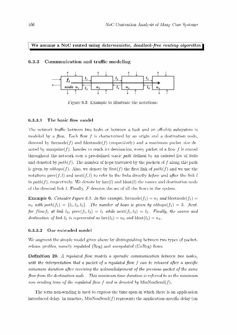
166 NoC Contention Analysis of Many Core Systems
We assume a NoC routed using deterministic, deadlock-free routing algorithm
6.3.3 Communication and tra�c modeling
f1 l1
l2 node n1 n2 n3
l3
l6 n4
l5
l4
Figure 6.3: Example to illustrate the notations:
6.3.3.1 The basic �ow model
The network tra�c between two tasks or between a task and an o�-chip subsystem is
modeled by a �ow. Each �ow f is characterized by an origin and a destination node,
denoted by fsrcnode(f) and fdestnode(f) (respectively) and a maximum packet size de-
noted by maxpsize(f). Inorder to reach its destination, every packet of a �ow f is routed
throughout the network over a pre-de�ned static path de�ned by an ordered list of links
and denoted by path(f). The number of hops traversed by the packets of f along this path
is given by nbhops(f). Also, we denote by first(f) the �rst link of path(f) and we use the
notations prev(f, l) and next(f, l) to refer to the links directly before and after the link l
in path(f), respectively. We denote by lsrc(l) and ldest(l) the source and destination node
of the directed link l. Finally, F denotes the set of all the �ows in the system.
Example 6. Consider Figure 6.3. In this example, fsrcnode(f1) = n1 and fdestnode(f1) =
n4 with path(f1) = {l1, l3, l5}. The number of hops is given by nbhops(f1) = 3. Next,
for flowf1 at link l3, prev(f1, l3) = l1 while next(f1, l3) = l5. Finally, the source and
destination of link l5 is represented as lsrc(l5) = n3 and ldest(l5) = n4.
6.3.3.2 Our extended model
We augment the simple model given above by distinguishing between two types of packet-
release pro�les, namely regulated (Reg) and unregulated (UnReg) �ows.
De�nition 20. A regulated �ow models a sporadic communication between two nodes,
with the interpretation that a packet of a regulated �ow f can be released after a speci�c
minimum duration after receiving the acknowledgement of the previous packet of the same
�ow from the destination node . This minimum time duration is referred to as the minimum
non-sending time of the regulated �ow f and is denoted by MinNonSend(f).
The term non-sending is used to express the time span in which there is an application
introduced delay. In practice, MinNonSend(f) represents the application-speci�c delay (on
6.4 Input Tra�c Characterization Functions 167
the core) before another packet can be generated: it may be an explicitly de�ned waiting
phase or time spent for processing. A stream of video frames which must be transferred
to an o�-chip graphic controller is an example of a regulated �ow.
De�nition 21. An unregulated �ow, models an aperiodic communication between two
nodes: the source node can release a packet at any instant in time after the receipt of its
previous packet has been acknowledged, i.e., for all unregulated �ows f , MinNonSend(f) is
null.
Data transfers between a task and the system memory at arbitrary times due to random
cache misses serves as an example of unregulated �ows. It is important to re-iterate that
our model inherently assumes �blocking� communication: any packet of a given �ow can
be generated only after the receipt of the acknowledgement of the previous packet.
6.4 Input Tra�c Characterization Functions
In this section, we introduce two functions associated with each �ow, namely the minimum
inter-release time function and the maximum packet release function.
6.4.1 The minimum Inter-Release Time Function
De�nition 22. The Minimum Inter-Release Time function MinInterRel(f) of a �ow f is
the minimum time gap between two consecutive packets released by f .
Speci�cally, if p1 and p2 are two consecutive packets generated by �ow f , then MinInterRel(f)
is the sum of (i) the minimum time needed to deliver and acknowledge p1 � sometimes
referred to as the round-trip time of p1 � and (ii) the application-speci�c minimum de-
lay that must elapse before the release of p2, i.e., MinNonSend(f). We then compute
MinInterRel(f) as:
MinInterRel(f) = MinDest(f) + MinDest(ack) + MinNonSend(f) (6.1)
where MinDest(f) is the minimum time taken by a packet of f to travel from its source
fsrcnode(f) to its destination fdestnode(f). Note that MinInterRel(f) di�ers from MinNonSend(f)
as it also includes the minimum time needed to send a packet of �ow f and receive its
corresponding acknowledgement. As a direct consequence of the need for acknowledging a
packet, the following property holds.
Property 3. No two packets of the same �ow f can reach a given router separated by a
time gap of less than MinInterRel(f) time units.
Note that these parameters are computed in isolation (i.e. without any contention from
the other �ows). Since the objective is to determine the WCTT of a given packet (say
p), we must be able to capture the worst-case scenario in which the blocking �ows can

168 NoC Contention Analysis of Many Core Systems
cause maximum interference to any packet of the analyzed �ow. We must therefore have
a parameter which represents a lower-bound on the inter-release time of all these blocking
�ows and so a lower-bound on MinDest(f) for all �ows f ∈ F . We shall use the following
result.
De�nition 23. For the wormhole routing technique, the minimum time-to-destination
MinDest(f), for any given �ow f ∈ F , is given by
MinDest(f) = nhops(f)× (dsw + dacross) +minpsize(f)
C(6.2)
where dacross is the time for a �it to be read from an input bu�er, traverse the crossbar (the
switch) and reach the storage at the input of a neighboring switch.
The above equation can be interpreted as follows. The term nhops(f) denotes the
number of hops that the �rst (header) �it of the packet of f traverses while travelling from
its source to destination. While traversing the network, the �rst �it locks down all the
output ports on its path and at each intermediate switch, it incurs an arbitration delay of
dsw and a time of dacross to traverse the crossbar. In our model, dacross also accounts for the
maximum time it takes to transfer �ow-control tokens between the routers. Once this �rst
�it reaches the destination, all the traversed output ports from its source to its destination
have been locked down and the entire packet of size minpsize(f) can travel over the network
of capacity C, which requires minpsize(f)/C time units. Hereafter, Equation (6.2) will be
used as the value of MinDest(f).
6.4.2 The Maximum Packet-Release Function
De�nition 24. The Maximum Packet Release Function MaxPcktRel(f, t) of a �ow f
provides an upper-bound on the number of packets that f can generate in a time interval
of length t.
This function is computed considering that the task (initiating the �ow) is run in
isolation, i.e., without any contention from other packets on the network and hence can
be determined at design time. Methods to compute an upper bound on the number of
requests issued by a task in a given time interval have been proposed by [91], [80] and [79].
For regulated �ows, the maximum packet release function can be expressed based on
the minimum inter-release time of the given �ow as in Equation (6.3), since their minimum
non-sending time is clearly de�ned and integrated into their minimum inter-release time.
MaxPcktRel(f, t) =
⌈t
MinInterRel(f)
⌉(6.3)
However, for unregulated �ows, computing MaxPcktRel() with the same approach may
lead to an over-estimated number of packets, especially for large values of t. To overcome
this pessimism in the computation, we can apply the method proposed in [91]. Although

6.5 Conceptual description of existing RC based methods 169
the exact time-instants at which unregulated �ows generate packets are not known, these
methods calculates this parameter by instrumenting the task code at di�erent sampling
points when the task executes in isolation and uses this information to derive an upper
bound on the maximum number of packets it can generate in any time interval of dura-
tion t. Note that the MaxPcktRel(f, t) function roughly corresponds to the arrival curve
abstraction used in network calculus theory.
6.5 Conceptual description of existing RC based methods
f3
f2
f1
l1
l4
l6
l5
l3
node n1
n2 n3 n4
l9
l2
l8
l7
Figure 6.4: Example to illustrate the approach in [146]
To understand the concepts behind the recursive calculus based method, we present an
algorithm to compute an upper bound on the traversal time of a packet of �ow f from its
source to the destination node. This will represent the approach proposed by Ferrandiz et.
al [146] and is conceptually similar to that of Rehmati et.al [145].
Let us consider the part of Figure 6.4. There are four nodes n1, n2, n3, n4 and three
�ows: f1, f2 and f3. All the �ows terminate at the core n4. Flow f1 originates in n1 and
the source nodes of f2 and f3 are not speci�ed in this example.
Let us compute the WCTT of �ow f1 for which fsrcnode(f) = n1, fdestnode(f) = n4
with path(f) = {l1, l6, l9} denoting the links that it traverses from the source to the
destination. The process commences by invoking the function d(f1, l1) (Algorithm 8).
Since link l1 is the �rst link in the path of �ow f1, it could be blocked only if other
�ows generated by its source (core n1) have to transit �rst. This particular case has been
handled in earlier methods but in contrast to their approach, we assume that the core
stalls while waiting for a given packet transmission to be completed before initiating a new
transmission. Therefore, under this assumption, a �ow f issued from one core can never
be blocked by another �ow issued from the same core and the �rst �it of the packet is
directly transferred to the (top) input port of the switch n2. Thus, the algorithm directly
calls the function d(f1, l6) at line 1. At this stage, the �ow f1 traverses via link l1 and next
passes through l6 via node n2.
The set of potential blocking links comprises those previously unexplored links for which
the destination matches with the current destination of the analyzed link. Accordingly at

170 NoC Contention Analysis of Many Core Systems
Algorithm 8: d(f, l)
input : a �ow f , a link loutput: WCTT of f , starting from link l, to the destination.// there cannot be any contention on the first link.
1 if l = first(f) then return d(f,next(f, l)) ;/* Header flit reaches end of path and the entire packet transits */
2 if l = null then return maxpsize(f)C ;
/* Determine the set of links excluding prev(f, l) and whose destination
node is lsrc */
3 BL← {lin ∈ L | lin 6= prev(f, l) ∧ ldest(lin) =lsrc(l)};4 foreach lin ∈ BL do
/* Determine the set of flows fin that use link lin and have l as the
next link */
5 Ulin ← {fin ∈ F | lin ∈ path(fin) ∧ next(fin, lin) = l};6 end
7 delay←∑lin∈BL
maxfin∈Ulin
{dsw + dacross + d(fin,next(fin, l))};
8 return delay +dsw + dacross + d(f,next(f, l)) ;
line 3, the algorithm computes the set of links, BL, connected to the other input ports of
n2 (i.e., the links excluding l1). Here, BL = {l3, l4, l5}.Then, for each of the links lin ∈ BL, the algorithm determines the set Ulin of blocking
�ows which pass consecutively through the next link in the path of the analyzed �ow i.e.,
l6. Here Ul4 = {f2} and the other sets (Ul3 , Ul5) do not have �ows matching the criterion
stated above and are therefore empty. Note that exactly one blocking �ow of each set Ulinmay block f1 since the switch follows a round-robin arbitration mechanism. Therefore,
to maximize the delay, for each link lin in BL, the algorithm explores all the �ows fin in
Ulin by recursively invoking d(fin, next(fin, l)) and then chooses the �ow which maximizes
the delay in line 7. It then computes the cumulative delay by summing up the maximum
delays obtained for each lin ∈ BL. After the blocking �ows are allowed to progress at
the current link, the �ow being analyzed, f1 can progress to its next link. At line 8,
the algorithm returns the cumulative delay computed in line 7 plus the time for the �ow
f1 to traverse through n2 (i.e., dsw), plus the delay su�ered by f1 in the next hop, i.e.,
d(f1, next(f1, l6)) = d(f1, l9). Notice that at line 2, if l = null, then it implies that the
�ow f has reached its destination. In this case, the packet of f is fully transmitted, which
requires, in the worst-case, maxpsize(f)C time units.
6.6 Proposed method for tighter WCTT
Inorder to compute a tighter WCTT, we �rst explore the sources of pessimism in the
previous approach and then describe the methods to deal with it.

6.6 Proposed method for tighter WCTT 171
6.6.1 Sources of Pessimism
Although the computation presented in the previous section is correct and terminates
within a reasonable computation time (as shown by [146]), we identi�ed two main sources
of pessimism. Inorder to highlight this pessimism, we constructed a computation tree as
shown in Figure 6.5 based on Algorithm 8. In this tree, each recursive call to the function
d(f, l), with l 6= null, is a (non-leaf) node of the tree and each call to d(f,null) is a leaf
node. Algorithm 8 traverses this computation tree in a pre-ordered depth-�rst manner:
�rst the root node is visited and then each of the children are visited, from the left to the
right.
As seen in Figure 6.5, the order in which the leaf nodes of the computational tree are
reached re�ects the following scenario. The �ow f1 is delayed because f2 goes �rst through
l6 (step À). f2 is then blocked by f3 at node n3. Once f3 has reached the core n4, its
whole packet is transferred to n4, hence adding maxpsize(f3)/C to the delay (step Á, the
�rst �leaf�). Then f2 �ows and reaches the core n4 (step Â), followed by f1 which passes
through n2 but gets blocked by another �ow of f3 in n3. This second �ow of f3 passes �rst
(step Ã) and �nally f1 can progress to its destination (step Ä).
As a conclusion, the scenario considered by the computation of d(f1, l1) assumes that f3
blocks the �ow f1 twice before it �nally reaches the core n4. These multiple blockings may
not be possible for several reasons and can lead to an overestimation of the WCTT. In the
next subsection we explore these reasons which we refer to as the �sources of pessimism�
and propose methods to overcome them.
6.6.2 Network-level Pessimism
The basic premise behind earlier approaches was the assumption that every �ow injects
tra�c continuously into the network, thereby assuming that for all �ows, the packets do not
expect any response and have no temporal constraints on their generation. In practice, the
application initiating a �ow may dictate that two consecutive packets cannot be generated
separated by less than a minimum time gap (given by the MinInterRel() functions). As
+
d(f1, l6)
d(f1, l1)
+ + +
¿
¡ ¬ √ ƒ
dsw + d(f2, l9) dsw + d(f1, l9)
dsw + d(f3, null) dsw + d(f2, null) dsw + d(f1, null)
maxpsize(f3)
C
maxpsize(f2)
C
maxpsize(f1)
C
maxpsize(f3)
C
dsw + d(f3, null)
Figure 6.5: Computation tree of d(f1, l1).

172 NoC Contention Analysis of Many Core Systems
seen in the previous section, this minimum time gap cannot be null as it includes the
round-trip communication delay incurred due to the underlying network. In a large setup,
on ignoring these �minimum round-trip time� constraints, the delay incurred as a result
of these non-feasible contentions can cascade and increase in magnitude as the �ow path
unrolls, ultimately leading to highly pessimistic WCTT estimates.
In the example of Figure 6.4, it is seen that �ow f3 blocks f1 twice: once indirectly by
blocking f2 and once directly in step Ã. However, because of its round-trip time constraint
it may not be possible for �ow f3 to release a second packet by the time �ow f1 transits
through node n3. Thus by taking into account this constraint, the analysis of the delay
incurred by f1 can be less pessimistic.
Inorder to tackle this source of pessimism, we introduce the notion of �current time�
during the computation. The current time is initialized to 0 at the beginning of the
analysis and it is then increased by dsw + dacross every time a �ow traverses a router and
by minpsize(fx)/C whenever a �ow fx reaches its destination. During the computation,
whenever a �ow fx traverses a router nk, the current time (denoted by t) is recorded and
used as a time-stamp for this traversal, i.e., a time-stamp is attached to the pair < fx, nk >.
Then, in the time interval [t, t+ MinInterRel(fx)], our proposed analysis will not recognize
�ow fx as a potentially blocking �ow in router nk as it is not possible for fx to have another
packet at an input port of nk in that interval of time in accordance with Property 3.
6.6.3 Task-level Pessimism
node nz
f1
node n1
many nodes in between
node ny
fx
node nx
ly
Figure 6.6: Example to illustrate task level pessimism
Intuitively, it may happen that many occurrences of a same �ow fx have to be con-
sidered by Algorithm 8 and none of them violates its MinInterRel(fx) constraint, i.e., at
every router on fx's path, every occurrence of fx is separated in time from the previous
one by at least MinInterRel(fx) time units.
A manifestation of this situation can be seen in the example of Figure 6.6. Let us
assume that the destination of the (dashed) �ow f1 is nz, and that nz is distantly located

6.7 The Branch and Prune Algorithm 173
from n1 (in terms of number of hops). In addition, consider a �ow fx from the core nxto nz. When computing the WCTT of f1, chances are high that Algorithm 8 invokes the
function d(fx, ly) a signi�cant number of times since it blocks all the �ows directed to nz.
As stated above, in such a case the �ow fx may never violate the constraint imposed by
MinInterRel(fx), as the distance between nx and nz is short, but at a given current time
t during the analysis it may be the case that the task which initiates fx is not able to
generate that many packets in the time interval [0, t]. As a result, Algorithm 8 may return
overly pessimistic WCTT estimates as it does not take into account the packet-release
pro�le speci�c to each task.
This work proposes to tackle this source of pessimism by extending the solution for
tackling the network-level pessimism. Instead of recording and maintaining a time-stamp
only for the last occurrence of every �ow fx in every router nk, we propose to save a
time-stamp for every occurrence of all the �ows in every router that they traverse. That
is, for each pair of �ow-router < fx, nr >, we maintain the number of occurences and the
corresponding list of time-stamps re�ecting all the time-instants at which fx has traversed
nk during the computation. Let us assume t0 is the time-stamp of the �rst occurrence of fxin nk. Then, at any current time t during the analysis, the �ow fx is deemed infeasible (and
hence cannot potentially block the analyzed �ow another time) if the number of recorded
occurences of fx in router nk exceeds MaxPcktRel(fx, t − t0), which as described earlier,
returns an upper bound on the number of packets generated by �ow fx in the speci�ed
time interval (t− t0).
6.7 The Branch and Prune Algorithm
This section introduces our �Branch and Prune� (BP) algorithm for calculating the WCTT
of a packet released by a �ow. While the basic principle of Algorithm 8, which consists of
recursively tracking the progression of all �ows throughout the network remains the same,
our method di�ers from this algorithm in two aspects:
1. It considers the extended �ow model presented in Section 6.3.3.2, in which the input
tra�c of the �ows are characterized with speci�c functions and
2. It incorporates the ideas described in Section 6.6 to reduce the task- and network-level
pessimism.
6.7.1 Overview of the Branch and Prune Algorithm
The basic principles of �ow progression remain the same as in Algorithm 8. At each link l
in the path of the analyzed �ow f , we �rst determine the set of all �ows that can potentially
block f by accessing l �rst. Then, we enumerate all possible interfering scenarios for that
link and we analyze each of them recursively. An interfering scenario is de�ned here as a
�ow sequence, i.e., an order of passage of the blocking �ows over the considered link.

174 NoC Contention Analysis of Many Core Systems
Figure 6.7: A simple example.
One of the main di�erences with Algorithm 8 is that we �rst branch-out, thereby enu-
merating all possible blocking �ow sequences, then we validate if the �ows in the sequence
can arrive, given their task constraints and thereby prune the infeasible �ows in each se-
quence. We compute and record the traversal times of these pruned sequences. Since the
tests for constraint compliance are applied early-on in the computation, the resulting search
space is greatly reduced. This is especially true for loaded networks wherein the impact
of indirect contention of certain �ows can cause the search space to grow exponentially. It
can be seen that pruning an infeasible �ow is equivalent to pruning the entire subtree of
�ows which would have blocked it later on (and would otherwise have to be explored by
the algorithm, thereby increasing the search space).
6.7.2 Concepts behind the algorithm
The main steps of our approach are described here with a simple example, illustrated in
Figure 6.7. Let us assume that f is the analyzed �ow which traverses on its kth hop
through the router nx along its path to the destination. This implies that interfering �ows
of an earlier hop may have been already analyzed for their delay in node nx.
6.7.2.1 Blocking Links and Flows
At every router in the path of f , we �rst determine the set of blocking links � those links
which terminate at the same node as the analyzed link. In the given example, assuming
that the analyzed link has router nx as its destination, the set BL of blocking links at
router nx is given by BL = {lp, lq}. Then, for each blocking link lin, we compute the
associated set Ulin of blocking �ows that can potentially block f in this router nx. Here,
Ulp = {fa, fb} and Ulq = {fc, fd}.At this stage, we still assume that all these blocking �ows have a packet to transmit
and are allowed to transmit it before the �ow f progresses.

6.7 The Branch and Prune Algorithm 175
6.7.2.2 List of Interfering Scenarios
During the computation, the progress of all �ows is ensured by the round-robin arbitration
policy applied at each intermediate router, which implies that at most one packet from
each of the blocking �ows can block the analyzed �ow f . At this phase, we are interested
in �nding the sequence of �ows progression over the network that will delay f for as long
as possible. To tighten the WCTT estimate by overcoming the limitations (sources of pes-
simism) presented earlier, at each router in the path of the analyzed �ow we �rst enumerate
all the possible �ow sequences (called �interfering scenarios� hereafter) that might block
it. Speci�cally, we denote by LIS the list of all possible �Local Interfering Scenarios� at
the current router, assuming that the currently analyzed �ow f is the last one allowed to
progress. That is, at router nx for example, LIS contains {fa, fc, f}, {fa, fd, f}, {fb, fc, f},{fb, fd, f}, {fc, fa, f}, {fc, fb, f}, {fd, fa, f}, {fd, fb, f} , {fa, f}, {fb, f}, {fc, f}, {fd, f},and {f}.
As a consequence of the pruning mechanism, there can be duplicate scenarios. These
duplicates, when present, are eliminated by the algorithm. All the remaining scenarios are
then investigated inorder to eliminate any possible timing anomalies and ensure the safety
of the algorithm. The necessity comes from the fact that any of the scenarios at a given
router cannot be implicitly discarded, as the local maximum at a given router may not
translate into the global maximum. For example, in the above LIS, we cannot ignore the
scenarios {fa, f} � intuitively we may conclude that among scenarios S1 = {fc, fa, f} andS2 = {fa, f}, the scenario S1 is more likely to contribute to the WCTT, but it may not
be so. In fact, S2 = {fa, f} may in the future progression, allow for �ows contributing to
a large interference to be included in the �nal WCTT while scenario S1 may prohibit it
thus leading to a timing anomaly and also leading to an unsafe WCTT.
We traverse this LIS and investigate each interfering scenario individually. When con-
sidering {fa, fc, f} for example, we �rst compute (recursively) the WCTT of fa, then the
WCTT of fc and �nally we allow f to progress to the next router on its path. However, be-
fore computing the WCTT of fa (and the same holds for fc later), we reduce the pessimism
of the computation by applying the two optimization mechanisms that determine whether
fa is �feasible�. Being infeasible implies that it is impossible for a given �ow to release
a packet at the given time, considering that it either released a packet too close in time
relative to its previous packet (thereby accounting for the network-level pessimism) or it
has already exceeded the upper bound on the number of packets it could possibly generate
from the beginning of the computation (task-level pessimism). If the �ow fa is declared
infeasible then it is removed from the currently considered interfering scenario {fa, fc, f}and the algorithm moves on with the next �ow fc of that scenario. As a side note, it can
be observed that removing fa from that scenario {fa, fc, f} yields the scenario {fc, f} andthus, the equivalent scenario {fc, f} listed in LIS will not have to be investigated again
later on. Thereby, removing �ows from a scenario is equivalent to pruning the resulting

176 NoC Contention Analysis of Many Core Systems
scenario from LIS, which considerably improves the time-complexity of this technique (as
well as the accuracy of the WCTT estimates) as discarding a single �ow from a scenario
automatically cuts o� a whole subtree from the computation tree.
6.7.2.3 Need for ordering
Since our approach considers the input �ow characteristics, the order in which �ows
progress cannot be ignored as it can lead to di�erent results.
Figure 6.8: Illustration to understand the need for ordering
We illustrate this with an example given in Figure 6.8. Consider two possible scenarios:
S1 = {fc, fd, fb, fd, fc, fa, fc, fd, f} and S2 = {fc, fd, fb, fc, fd, fa, fc, fd, f}. These two
scenarios only di�er in the order in which fc and fd block fa. However, notice that in S1
the �rst and the second appearance of fd are distanced only by fb, while the second and the
third appearance of fc are distanced only by fa. Conversely, in S2, any two appearances of
the same �ow are distanced by at least two other �ows. Depending on �ow characteristics,
in some cases the entire S2 might be feasible, while S1 would require the pruning of some
appearances of fc and/or fd. Thus, considering only S1 in the analysis may result in unsafe
worst-case estimates, and in order to capture the worst-case it is necessary to investigate
all possible �ow orderings at every traversed router.
Indeed, at a given router nx along f 's path, the list of interfering scenarios can be
computed as explained above but identifying which blocking �ows are infeasible within
each of these scenarios requires the knowledge of which �ows have already progressed (and
in which order) in the previously traversed routers, before f reaches nx. Without this
knowledge, our pruning mechanisms would not be able to determine whether a �ow listed
in an interfering scenario is feasible or not. This leads to the concept of �context� which is
key in our algorithm.
6.7.2.4 Notion of a �context�
Formally, a context is a snapshot of all the information characterizing a unique sequence
of �ow progressions throughout the network before a given �ow f reaches a given router
nx, including
1. the order in which the �ows have progressed over the network so far,

6.7 The Branch and Prune Algorithm 177
2. all the past occurrences and the associated timestamps of all these �ows in this �ow
sequence and
3. the delay incurred by f before it reaches nx
At a given router nx, for a given �ow f and context ctx, which (informally speaking)
re�ects the history of what happened in the network before that �ow f reached nx, we
explained above that every feasible blocking �ow of every interfering scenario of LIS in nxwill be allowed to progress from nx to its destination before the analyzed �ow f . Therefore,
it can be seen that the progression of each of these blocking �ows towards their destination
may in-turn generate a multitude of new contexts (more exactly, the progression of each
blocking �ow will make the current context ctx evolve in an unique way). Subsequently,
all these new contexts derived from ctx are investigated when f eventually progresses to
the next router on its path. At the end, the WCTT of f will be found by looking at all
the �ow sequences (i.e., the contexts) in which f �nally reaches its destination.
Algorithm 9: getMaxDelay(Flow f, Link l)input : a �ow f , a link loutput: WCTT of �ow f , starting from link l, to the destination.
1 StudiedFlow← f , ctx.scenario ← � �, ctx . delay← 0 ;2 ctxSet← getContexts(f, l, ctx) ;3 maxdelay← max∀ ctx∈ctxSet ctx .delay ;4 return maxdelay ;
6.7.3 Detailed Explanation of the Algorithm GetContexts()
Initially, the algorithm is invoked by Algorithm 9 with the following inputs: the �ow f to
be analyzed, the �rst link l on its path and an initial �context�. The initial context contains
an empty �ow sequence, a delay of zero, and past occurrences set to null. On arriving at a
router, the algorithm (line 10) computes the set of blocking links BL (as explained earlier)
and the corresponding blocking �ows (lines 11-13) incident on each of the links in BL.
Based on this information, the set LIS of Local Interfering Scenarios is computed (line 14)
as follows: LIS contains all permutations of �ow sequences in which (i) there is exactly
zero or one �ow from each set Ulin and (ii) the analyzed �ow f is appended to each of these
permutations.
Once the set LIS is computed, the algorithm investigates each of them. Let us revisit
the example in Figure 6.8. For each scenario in LIS, (line 16), e.g, {fa, fc, f}, the list
SCList will ultimately contain all the generated contexts arising from the execution of this
scenario. The investigation starts with the �rst �ow, here fa (line 18), and considers every
current context curCtx (line 19) that results in f reaching the link l. Remember that,
(because our extended model considers �ows with some timing constraints on their packet
generation) the interfering scenarios that can occur for a �ow f in a router nx depend on
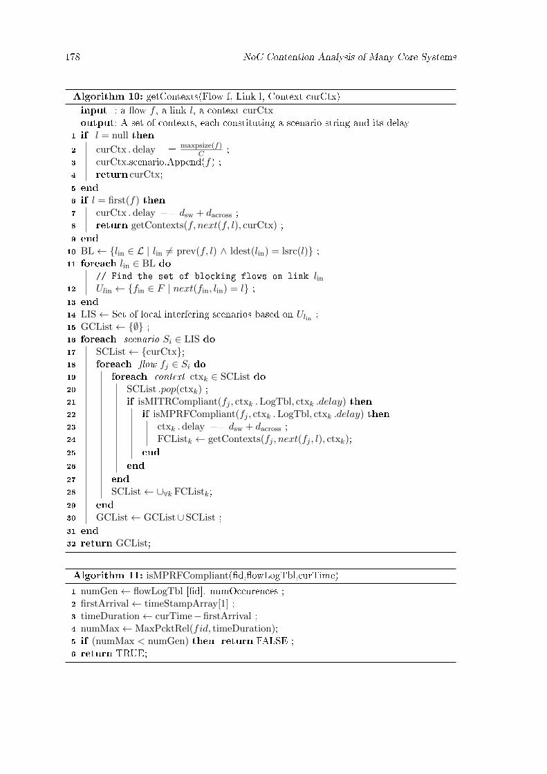
178 NoC Contention Analysis of Many Core Systems
Algorithm 10: getContexts(Flow f, Link l, Context curCtx)input : a �ow f , a link l, a context curCtxoutput: A set of contexts, each constituting a scenario string and its delay
1 if l = null then
2 curCtx .delay += maxpsize(f)C ;
3 curCtx.scenario.Append(f) ;4 return curCtx;5 end6 if l = first(f) then7 curCtx .delay += dsw + dacross ;8 return getContexts(f, next(f, l), curCtx) ;9 end
10 BL← {lin ∈ L | lin 6= prev(f, l) ∧ ldest(lin) = lsrc(l)} ;11 foreach lin ∈ BL do
// Find the set of blocking flows on link lin12 Ulin ← {fin ∈ F | next(fin, lin) = l} ;13 end14 LIS← Set of local interfering scenarios based on Ulin ;15 GCList← {∅} ;16 foreach scenario Si ∈ LIS do17 SCList← {curCtx};18 foreach �ow fj ∈ Si do19 foreach context ctxk ∈ SCList do20 SCList .pop(ctxk) ;21 if isMITRCompliant(fj , ctxk .LogTbl, ctxk .delay) then22 if isMPRFCompliant(fj , ctxk .LogTbl, ctxk .delay) then23 ctxk .delay += dsw + dacross ;24 FCListk ← getContexts(fj , next(fj , l), ctxk);25 end
26 end
27 end28 SCList← ∪∀k FCListk;29 end30 GCList← GCList∪SCList ;31 end32 return GCList;
Algorithm 11: isMPRFCompliant(�d,�owLogTbl,curTime)
1 numGen← flowLogTbl [�d]. numOccurences ;2 firstArrival← timeStampArray[1] ;3 timeDuration← curTime−firstArrival ;4 numMax← MaxPcktRel(fid, timeDuration);5 if (numMax < numGen) then return FALSE ;6 return TRUE;

6.8 A more e�cient algorithm: Branch, Prune and Collapse 179
Algorithm 12: isMITRCompliant(�d,�owLogTbl,curTime)
1 if (FirstOccurence(fid,flowLogTbl))||(curTime ≥ �d.NextfeasibleArrival) then// For the corresponding entry in the table
2 Increment numOccurences ;3 Append curTime to the timeStampArray ;4 Reset NextfeasibleArrival to curTime + MinInterRel(f) ;5 return TRUE ;6 end7 return FALSE ;
the order in which the previous �ows progressed through the network before f reaches nx.
Hence, whenever a �ow f reaches a router nx, all possible contexts have to be investigated
in order to determine all the future scenarios that could arise at router nx.
First, lines 21 and 22 check whether fa can legally block the analyzed �ow f considering
the time of its last arrival in the considered context (here, curCtx). If fa can arrive and
passes the round trip time test (line 21) as described in Algorithm 12, the task charac-
teristics of the �ow are checked. Speci�cally, line 22 checks if the task originating fa can
indeed generate that many packets in the time speci�ed by calling the function de�ned in
Algorithm 11. If both checks of lines 21 and 22 succeed, then fa is allowed to progress
in line 24, after updating the current context delay parameter (line 23). Ultimately, the
passage of fa returns a set of contexts (line 24), when �ow fa reaches its destination (which
is re�ected when its last link is null (lines 1-5) ).
All these returned contexts end with �ow fa reaching its destination and each one
corresponds to a di�erent scenario in the subsequent routers along the path of fa. All
these resulting contexts are added to the scenario list SCList (line 28) as they must all be
considered (line 17) while analyzing the next �ow fc of the current scenario. When all the
�ows of the currently considered interfering scenario have been considered, all the contexts
resulting from this scenario are added to the global list GCList (line 30). That list is �nally
returned (line 32), as it contains all the possible �ow sequence progressions in the routers
traversed by f after progressing through the link l, starting with the context curCtx. The
list GCList that is ultimately returned (to Algorithm 9) at the end of the analysis, contains
all possible scenarios in which f can reach its destination, with the corresponding delays.
Finally, Algorithm 9 selects the scenario with the highest delay to return an upper-bound
on the traversal time of the analyzed �ow f .
6.8 A more e�cient algorithm: Branch, Prune and Collapse
6.8.1 Description
The recursive calculus based method proposed by [146] scales well at the cost of providing
a very pessimistic WCTT. In contrast, the proposed branch and prune (BP) algorithm

180 NoC Contention Analysis of Many Core Systems
returns a very tight WCTT at the cost of a high time complexity and memory usage. The
reason for the improved computational e�ciency in the method by [146] is that it does
not carry any history of the previous �ows and only retains the maximum delay incurred
at each router. From the two extreme approaches it may be inferred that a hybrid solution
exists which can drop some history of the contexts (only) periodically while retaining the
maximum delay seen so far as the analysis progresses. Such an approach is explored in
this section.
As seen earlier, the identi�cation of infeasible scenarios in BP was possible due to the
explicit book-keeping of contexts of all investigated scenarios. The �Branch, Prune and
Collapse� (BPC) algorithm presented (conceptually) in this section is motivated by the
observation that, while the complexity of the BP algorithm is indeed exponential, for most
�ows, the number of scenarios to be considered is manageable (as seen in the experiments
of Section 6.9). To handle the corner cases (in terms of time complexity) we propose as a
trade-o�, a more general BPC algorithm with a tunable parameter that we term �Scenario
Information Retention Limit� (SIRL). The SIRL acts as a threshold on the number of
scenarios whose contexts are retained.
In the BP algorithm, all the investigated scenarios and their contexts are back prop-
agated and the algorithm proceeds by �rst pruning these investigated scenarios and then
combining them with the local scenarios and then allowing the next feasible �ow to
progress. As a deviant version of this algorithm, which is hereafter referred to as BPC,
when the number of investigated scenarios reaches a pre-set limit of SIRL, a dummy sce-
nario with a unique dummy �ow-id is created. The context of this scenario populates (i)
the delay �eld to the maximum of the delays of the investigated scenarios and (ii) the
other �elds, relating to the history information i.e the past occurrences, timestamps, etc to
NULL (or zero, as appropriate) � This marks the �collapse� phase of the BPC algorithm in
which a set of investigated scenarios is �collapsed� into a new single dummy scenario with
zero history information and a conservative delay estimate. As opposed to the branch and
prune algorithm, only this dummy scenario is back propagated to the higher nodes and
the algorithm gets back in to the branch and prune phase until the number of investigated
scenarios again exceeds SIRL, thereby triggering another collapse phase.
The necessity to create a new dummy scenario Note, that at any intermediate stage
of analysis, if the number of scenarios under investigation reaches the pre-set threshold i.e.,
the SIRL, a single scenario that will provably lead to the WCTT cannot be detected. That
is, during the collapse phase, from the set of the constituent collapsed scenarios, a speci�c
single scenario (containing a tightly coupled local maximum delay, �ow sequences and other
history information) cannot be speci�cally carried forward. This is due to the fact that
in the later analysis stages such a scenario with the local maximum might be subject to
pruning because of its �ow history and thereby not contribute to the global maximum delay.
Inorder to prevent this, we drop the history information (thereby reducing the chances of

6.8 A more e�cient algorithm: Branch, Prune and Collapse 181
Figure 6.9: Example for �Branch, Prune and Collapse�
further optimization due to the loss of history retained in the collapsed scenarios) while
only retaining the local maximum delay in a totally new dummy scenario. To summarize,
the BPC method thereby creates a dummy scenario which inherits the delay of the local
maximum, but drops the history of the �ows constituting that scenario (context).
6.8.2 An example to illustrate the BPC method
We illustrate the working of the BPC method with the example of the �ow-set presented
in Figure 6.9 (repeated here for readability) � let us analyze �ow f which traverses through
routers n1 and n2 to �nally reach its destination n3. As observed in Figure 6.9, �ows fcand fd can potentially block �ow f thrice: twice indirectly by blocking the passage of faand fb at n2 (fa and fb block f directly at node n1), and �nally directly at n2 during f 's
passage. Thus, fc and fd are promising candidates for pruning (lines 21 and 22 of Algo-
rithm 10). Additionally, let us assume that SIRL = 5. At node n1, BPC constructs the LIS
as LIS(f, n1) = 〈{fa, fb, f}, {fb, fa, f}, {fa, f}, {fb, f}, {f}〉 and it starts exploring the �rst
scenario {fa, fb, f}. At this time, the list SCList is reset to the current context (at line 17 of
Algorithm 10). Note, that the list SCList will ultimately contain all generated contexts aris-
ing from the execution of this scenario {fa, fb, f}, before being appended to the global list
of contexts GCList at line 30. Firstly, a recursive call is performed to node n2 with fa being
the analyzed �ow. This will result in a new LIS constructed at node n2 as LIS(fa, n2) =
〈{fc, fd, fa}, {fd, fc, fa}, {fc, fa}, {fd, fa}, {fa}〉. Similarly, LIS is generated for the �ow fb
at n2, resulting with LIS(fb, n2) = 〈{fc, fd, fb}, {fd, fc, fb}, {fc, fb}, {fd, fb}, {fb}〉.These scenarios are back-propagated to the node n1, and should be combined before f
progresses to n2 itself. As both LIS sets contain 5 elements, the combined set of scenarios
may contain 25 scenarios (5 contexts from fa combined with 5 from fb). It is obvious
that for extremely complex �ows, this back-propagation may produce a large number
of scenarios, resulting in a combinatorial explosion, which is the drawback of the BP
method. Given that SIRL = 5 in this example, the collapsing requirement is met. Those
25 scenarios are collapsed into a single one containing the dummy �ow fX and its delay
is set to maximum delay amongst the collapsed scenarios. When f �nally progresses to
n2 and encounters the blocking �ows fc and fd, the algorithm checks the history in its
sequence {fX , f} and since there is no prior information regarding fc and fd, the analysis
182 NoC Contention Analysis of Many Core Systems
considers that these two �ows are arriving for the �rst time and thus allows them to pass
and interfere. The resulting scenarios would be {fX , fc, fd, f}, {fX , fd, fc, f}, {fX , fc, f},{fX , fd, f} and {fX , f}. In contrast, BP would have retained the information regarding all
scenarios, thus prohibiting the second interference caused by fc and fd, but at the expense
of investigating 25× 5 = 125 scenarios.
This example clearly brings forth two main principles:
1. The loss of past information can reduce the chances of pruning infeasible scenarios.
2. The number of scenarios to be explored signi�cantly decreases with the decease in
the SIRL parameter � and more speci�cally in loaded networks in which the context
of large scenarios have to be back-propagated to higher level nodes and combined to
evolve the �nal scenarios.
Conceptually, a SIRL set to∞ implies BPC = BP while at the other end, a SIRL set to
1 tends towards obtaining the WCTT using the method proposed by Ferrandiz et. al [146],
where no information about the past occurrence of any �ow is retained. This approach is
provided to the designer to handle the comparably small number of cases in which the BP
algorithm may be ine�cient. To formally validate the �exibility this o�ers, it will be seen
in the experiment sections how lower SIRL will compute bounds tending towards those
computed by Ferrandiz et. al [146], while with higher SIRLs we will have tighter WCTTs
computed by BP. With this parameter, the system designer has the �exibility to trade-o�
computation time vs. pessimism in the computed WCTT.
6.8.3 Proof of Safety of �Branch, Prune and Collapse� (BPC) algorithm
In this section, we explain why the BPC method, by discarding some history informa-
tion upon reaching the SIRL threshold, may output more pessimistic WCTT estimates
compared to BP, but will under no circumstance lead to an unsafe WCTT estimate.
Let us denote by wcs the scenario (�ow sequence) leading to the WCTT at run time
which is by de�nition a feasible scenario. Inorder to prove that BPC is safe, we must prove
that the BPC method does not eliminate this scenario wcs from the set of investigated
scenarios � the method should never return aWCTT which is lower than that corresponding
to the traversal time of wcs.
Firstly, it should be noted that, if we disable the two pruning mechanisms at lines 21
and 22 of Algorithm 10 and if SIRL is set to ∞, then our BPC algorithm boils down to
an exhaustive enumeration of all possible scenarios at each router, and thus considers all
possible blocking scenarios in the context of the analyzed �ow (brute-force approach which
is inherently safe). The pruning mechanisms of lines 21 and 22 use the precedence and
time stamp information to identify some infeasible �ow sequences and reduce the list of
scenarios that need to be explored and facilitates the objective of obtaining tighter WCTTs.
By de�nition, wcs is a feasible �ow sequence and therefore, it will not be eliminated by
these pruning techniques.

6.9 Simulations and Results 183
Given the loss of history information, the BPC method is unable to identify as many
infeasible scenarios as the BP method. These infeasible scenarios (�ow sequences) have
�ows that actually cannot occur at run time due to the task properties and hence add
to extra-delays and bloat up the traversal time. Eventually, the set of scenarios explored
will consider the set of feasible scenarios which includes wcs but will also include some
infeasible scenarios, which are not identi�ed due to loss of previous history and precedence
information. Finally, on taking the maximum traversal time of all the scenarios, the method
will return a value which is higher than or equal to the WCTT corresponding to wcs �
hence the method is safe.
To summarize, BP investigates all feasible (including the wcs) and infeasible scenarios
and prunes some infeasible scenarios by retaining the history information, and thereby is
safe. BPC investigates all feasible and infeasible scenarios and since it looses some history
information, it is capable of pruning only a subset of the infeasible scenarios that could be
pruned by BP and as a consequence is still safe but more pessimistic.
6.8.4 Proof of termination of Algorithm GetContexts (Algo. 10)
The system is modeled as a graph G(N ,L) with �nite sets of nodes and bi-directional links
and a set F of �ows. Let S be the set of pairs 〈f, `〉, with f ∈ F and ` ∈ L, such that
〈f, `〉 ∈ S if and only if ` ∈ path(f). Since | L | and | F | are �nite, it holds that | S | is�nite as well. A progress of a �ow f from a link ` to a subsequent link `′ on its path is
equivalent to the progress from the pair 〈f, `〉 to the pair 〈f, `′〉. If a �ow f ′ blocks �ow
f on the link `, it corresponds to the progress from the pair 〈f, `〉 to the pair 〈f ′, `〉 ∈ S.For a given �ow f and a current link `, the algorithm progresses in a forward manner to
the next link next(f, `) in the path of the �ow f by invoking the function getContexts()
at lines 8 and 24. Starting from any pair 〈f, `〉 ∈ S (i.e. with f and ` as input), our
algorithm investigates all the pairs, i.e. set of inputs, 〈f ′, next(f ′, `)〉 with f ′ 6= f as a
consequence of the round-robin arbitration policy. Then, the algorithm repeats the same
(in a recursive manner) for each of these pairs 〈f ′, next(f ′, `)〉 and, as a consequence of
the deadlock-free property of XY routing, we know that the initial pair 〈f, `〉 will never bere-visited. Additionally, since all the explored contexts are popped in line 20, the queue of
pending scenarios is emptied and the algorithm eventually terminates.
6.9 Simulations and Results
We conducted several experiments with the dual objectives of comparing our method with
the approach in [146] and studying the impact of varying di�erent parameters on the
WCTT of analyzed tasks. The simulation parameters have been summarized in the fol-
lowing table:

184 NoC Contention Analysis of Many Core Systems
Network Size 8*8 meshRouting and switching mechanism XY Routing, round robin arbitration
Router switching delay and transfer delay 1ns and 3ns (in-line with SCC [24]))Packet size and channel capacity 512 bytes, 1 Gbps
Platform details Intel dual-core & Java (Max heap-size:4GB)
6.9.1 Comparison of BPC with the Approach of Ferrandiz et. al [146]
As the improvements cannot be quanti�ed in the general sense, since they are highly �ow-
set speci�c, we performed experiments on a wide range of di�erent �ow-sets in order to
understand the trends and the ranges of improvement achieved by employing the proposed
approach.
Test 1: Network with moderate number of �ows: We generated 200 random �ow-
sets, each having 64 �ows. The �ows originate from each tile but terminate at a random
destination. The minimum inter-arrival time is a randomly generated parameter, varying
between 5 to 20 microseconds. We computed the upper-bounds on the WCTT of each
�ow using both the approaches and compared the results. For our approach, we selected
a SIRL = 10000.
Inorder to quantify the range of improvements, we computed a metric which we refer
to as the �Percentage Improvement Ratio� (PIR) given by (dU − d10000O ) ∗ 100/dU , where
dU denotes the upper-bound on WCTT returned by the approach in [146] which we also
refer to as unoptimized WCTT, and d10000O is the value returned by our algorithm for
SIRL = 10000, which we call optimized WCTT. Therefore a PIR = 25% implies that our
approach provided 25% lower (i.e. tighter) WCTT upper-bound.
Figure 6.10a summarizes our �ndings. We observed that for 31.84% of the �ows, the
bounds computed by both methods are equal, that is d10000O = dU and PIR = 0%. We
have also demonstrated the percentage of �ows and the improvement they achieved, in
order to provide a deeper insight into the performance of our algorithm. As evident from
Figure 6.10a, 1.29% of the �ows had a PIR in the range (1 − 10%), 13.22% in the range
(11 − 20%) and so on. At the high end of the PIR scale, 3.55% of the analyzed �ows
returned 71− 100% tighter WCTT bounds.
The WCTT* parameter: If the computation terminates with the number of investi-
gated scenarios not exceeding SIRL (implying that no collapses occur during the entire �ow
analysis), the method returns a value of the traversal time as would be computed by BP
� we denote this result by WCTT*. In other words, all possible scenarios were analyzed
and the one inducing the highest worst-case delay was recognized. Conversely, in cases
when collapses occur, the returned WCTT presents only an upper-bound on the worst-
case delay, without any additional details on how tight that bound is. When viewed from
that perspective, the approach in [146] presents a special case of the proposed approach
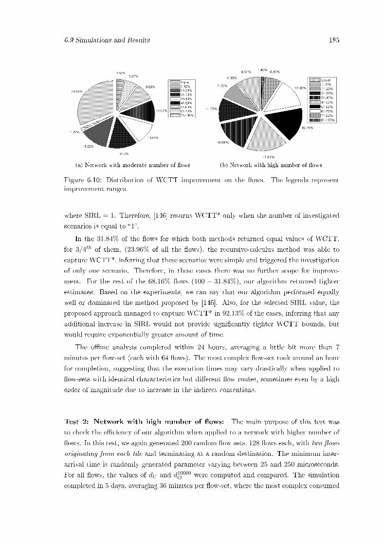
6.9 Simulations and Results 185
(a) Network with moderate number of �ows (b) Network with high number of �ows
Figure 6.10: Distribution of WCTT improvement on the �ows. The legends representimprovement ranges.
where SIRL = 1. Therefore, [146] returns WCTT* only when the number of investigated
scenarios is equal to �1�.
In the 31.84% of the �ows for which both methods returned equal values of WCTT,
for 3/4th of them, (23.96% of all the �ows), the recursive-calculus method was able to
capture WCTT*, inferring that these scenarios were simple and triggered the investigation
of only one scenario. Therefore, in these cases there was no further scope for improve-
ment. For the rest of the 68.16% �ows (100 − 31.84%), our algorithm returned tighter
estimates. Based on the experiments, we can say that our algorithm performed equally
well or dominated the method proposed by [146]. Also, for the selected SIRL value, the
proposed approach managed to capture WCTT* in 92.13% of the cases, inferring that any
additional increase in SIRL would not provide signi�cantly tighter WCTT bounds, but
would require exponentially greater amount of time.
The o�ine analysis completed within 24 hours, averaging a little bit more than 7
minutes per �ow-set (each with 64 �ows). The most complex �ow-set took around an hour
for completion, suggesting that the execution times may vary drastically when applied to
�ow-sets with identical characteristics but di�erent �ow routes, sometimes even by a high
order of magnitude due to increase in the indirect contentions.
Test 2: Network with high number of �ows: The main purpose of this test was
to check the e�ciency of our algorithm when applied to a network with higher number of
�ows. In this test, we again generated 200 random �ow-sets, 128 �ows each, with two �ows
originating from each tile and terminating at a random destination. The minimum inter-
arrival time is randomly generated parameter varying between 25 and 250 microseconds.
For all �ows, the values of dU and d10000O were computed and compared. The simulation
completed in 5 days, averaging 36 minutes per �ow-set, where the most complex consumed

186 NoC Contention Analysis of Many Core Systems
������������������������������������������������������
������������������������������������������������������
���������������������������������������������������������������������������������
���������������������������������������������������������������������������������
���������������������������������������������������������������������������������
���������������������������������������������������������������������������������
������������������������������������������������������
������������������������������������������������������
���������������������������������������������������������������������������������
���������������������������������������������������������������������������������
���������������������������������������������������������������������������������
���������������������������������������������������������������������������������
���������������������������������������������������������������������������������
���������������������������������������������������������������������������������
������������������������������������������������������
������������������������������������������������������
������������������������������������������������������
������������������������������������������������������
���������������������������������������������������������������������������������
���������������������������������������������������������������������������������
���������������������������������������������������������������������������������
���������������������������������������������������������������������������������
������������������������������������������������������
������������������������������������������������������
���������������������������������������������������������������������������������
���������������������������������������������������������������������������������
���������������������������������������������������������������������������������
���������������������������������������������������������������������������������
���������������������������������������������������������������������������������
���������������������������������������������������������������������������������
������������������������������������������������������
������������������������������������������������������
������������������������������������������������������
������������������������������������������������������
���������������������������������������������������������������������������������
���������������������������������������������������������������������������������
���������������������������������������������������������������������������������
���������������������������������������������������������������������������������
������������������������������������������������������
������������������������������������������������������
������������������������������������������������������������������������������������
������������������������������������������������������������������������������������
���������������������������������������������������������������������������������
���������������������������������������������������������������������������������
������������������������������������������������������������������������������������
������������������������������������������������������������������������������������
��������������������������������������������������������
��������������������������������������������������������
����������������������������
����������������������������
������������������������������������������
������������������������������������������
���������������������������������������������
���������������������������������������������
����������������������������
����������������������������
���������������������������������������
���������������������������������������
���������������������������������������
���������������������������������������
������������������������������������������
������������������������������������������
����������������������������
����������������������������
����������������������������
����������������������������
������������������������������������������
������������������������������������������
������������������������������������������
������������������������������������������
����������������������������
����������������������������
���������������������������������������
���������������������������������������
������������������������������������
������������������������������������
���������������������������������
���������������������������������
����������������������
����������������������
������������������������������
������������������������������
������������������������������������������
������������������������������������������
���������������������������������������
���������������������������������������
����������������������
����������������������
���������������������������������
���������������������������������
������������������������������
������������������������������
���������������������������
���������������������������
������������������
������������������
����������������������������
����������������������������
���������������������������������������
���������������������������������������
������������������������������
������������������������������
����������������
����������������
���������������������������
���������������������������
���������������������
���������������������
���������������������
���������������������
��������������
��������������
����������������������������
����������������������������
������������������������������������
������������������������������������
���������������������
���������������������
������������
������������
������������������
������������������
���������������
���������������
������������������
������������������
����������
����������
����������������������������������������������������
����������������������������������������������������
������������������������������������������������
������������������������������������������������
���������������������������
���������������������������
����������������
����������������
���������������������
���������������������
���������������������
���������������������
���������������
���������������
����������
����������
����������������������������������������
����������������������������������������
��������������������
��������������������
���������������
���������������
������������
������������
���������������
���������������
��������������������
���������������
���������������
����������������
������������
������������
���������
���������
������������
������
������
������������
���������
���������
���������
���������
��������
��������
��������
����
������������
��������
������������
������������
��������
0%
20%
40%
60%
80%
100%
Lim4 Lim20 Lim100 Lim200 Lim1,000 Lim2,000 Lim4,000 lim10,000
Per
cen
tage
of
flow
s
91−100% improvement
81−90% improvement
71−80% improvement
61−70% improvement
51−60% improvement
41−50% improvement
31−40% improvement
21−30% improvement
11−20% improvement
1−10% improvement
No improvement
������������������������������������������������������
������������������������������������������������������
���������������������������������������������������������������������������������
���������������������������������������������������������������������������������
���������������������������������������������������������������������������������
���������������������������������������������������������������������������������
������������������������������������������������������
������������������������������������������������������
���������������������������������������������������������������������������������
���������������������������������������������������������������������������������
���������������������������������������������������������������������������������
���������������������������������������������������������������������������������
���������������������������������������������������������������������������������
���������������������������������������������������������������������������������
������������������������������������������������������
������������������������������������������������������
������������������������������������������������������
������������������������������������������������������
���������������������������������������������������������������������������������
���������������������������������������������������������������������������������
���������������������������������������������������������������������������������
���������������������������������������������������������������������������������
������������������������������������������������������
������������������������������������������������������
���������������������������������������������������������������������������������
���������������������������������������������������������������������������������
���������������������������������������������������������������������������������
���������������������������������������������������������������������������������
���������������������������������������������������������������������������������
���������������������������������������������������������������������������������
������������������������������������������������������
������������������������������������������������������
������������������������������������������������������
������������������������������������������������������
���������������������������������������������������������������������������������
���������������������������������������������������������������������������������
���������������������������������������������������������������������������������
���������������������������������������������������������������������������������
������������������������������������������������������
������������������������������������������������������
������������������������������������������������������������������������������������
������������������������������������������������������������������������������������
���������������������������������������������������������������������������������
���������������������������������������������������������������������������������
������������������������������������������������������������������������������������
������������������������������������������������������������������������������������
��������������������������������������������������������
��������������������������������������������������������
����������������������������
����������������������������
������������������������������������������
������������������������������������������
���������������������������������������������
���������������������������������������������
����������������������������
����������������������������
���������������������������������������
���������������������������������������
���������������������������������������
���������������������������������������
������������������������������������������
������������������������������������������
����������������������������
����������������������������
����������������������������
����������������������������
������������������������������������������
������������������������������������������
������������������������������������������
������������������������������������������
����������������������������
����������������������������
���������������������������������������
���������������������������������������
������������������������������������
������������������������������������
���������������������������������
���������������������������������
����������������������
����������������������
������������������������������
������������������������������
������������������������������������������
������������������������������������������
���������������������������������������
���������������������������������������
����������������������
����������������������
���������������������������������
���������������������������������
������������������������������
������������������������������
���������������������������
���������������������������
������������������
������������������
����������������������������
����������������������������
���������������������������������������
���������������������������������������
������������������������������
������������������������������
����������������
����������������
���������������������������
���������������������������
���������������������
���������������������
���������������������
���������������������
��������������
��������������
����������������������������
����������������������������
������������������������������������
������������������������������������
���������������������
���������������������
������������
������������
������������������
������������������
���������������
���������������
������������������
������������������
����������
����������
����������������������������������������������������
����������������������������������������������������
������������������������������������������������
������������������������������������������������
���������������������������
���������������������������
����������������
����������������
���������������������
���������������������
���������������������
���������������������
���������������
���������������
����������
����������
����������������������������������������
����������������������������������������
��������������������
��������������������
���������������
���������������
������������
������������
���������������
���������������
��������������������
���������������
���������������
����������������
������������
������������
���������
���������
������������
������
������
������������
���������
���������
���������
���������
��������
��������
��������
����
������������
��������
������������
������������
��������
0%
20%
40%
60%
80%
100%
Lim4 Lim20 Lim100 Lim200 Lim1,000 Lim2,000 Lim4,000 lim10,000
Per
cen
tag
e o
f fl
ow
s
91−100% improvement
81−90% improvement
71−80% improvement
61−70% improvement
51−60% improvement
41−50% improvement
31−40% improvement
21−30% improvement
11−20% improvement
1−10% improvement
No improvement
Figure 6.11: Our proposed approach with varying SIRL vs. method by [146]. The �Lim�on the x axis denotes the threshold limit (SIRL) followed by the value
around 3 hours, demonstrating that our approach is scalable and applicable to practical
scenarios involving hundreds of concurrent �ows.
As in the previous test-set, the PIR metric is used here to quantitatively express the
improvements of the proposed method over the recursive calculus method by Ferrandiz et.
al [146] and the results are re�ected in Figure 6.10b. We observed that for 9.17% of the
�ows, no improvements were made (PIR = 0%). For most of the �ows without improve-
ment (8.11% among the 9.17% �ows) the approach by Ferrandiz et. al [146] managed to
capture WCTT*, with the same conclusion that for these simple, one-scenario cases no
improvements were possible. For the rest, i.e. 90.73% of the analyzed �ows, it holds that
d10000O < dU , that is the upper-bound on the worst-case of the analyzed �ows was tighter
with our approach and the distribution is re�ected in Figure 6.10b. It is interesting to see
that more than 13% of the �ows showed an improvement of 61−70%, while more than 8%
of the �ows show an improvement greater than 70%. Due to more complex tra�c patterns
resulting from increased amount of tra�c, our approach with SIRL = 10000 recognized
WCTT* for 41.71% of the �ows, which is signi�cantly smaller when compared with the
same of moderately loaded network. This suggests that the improvements can be achieved
by increasing SIRL, but at the expense of additional computational complexity and mem-
ory consumption. Although the proposed approach takes a longer computation time, it
clearly dominates the recursive calculus method in terms of obtaining tighter results. The
selection of SIRL creates a trade-o� between the computation time and the accuracy of
the analysis.
Test 3: Impact of SIRL onWCTT estimates: The objective of this set of experiment
is to understand the impact of varying SIRL on the computed WCTT. The general intuition
is that retaining more information about the scenarios provides more opportunities for
eliminating invalid scenarios and therefore leads to tighter estimates. To validate this idea,
we implemented our algorithm and executed it, by providing a di�erent value of SIRL for
each run and compared them against the results obtained by the approach in [146]. The
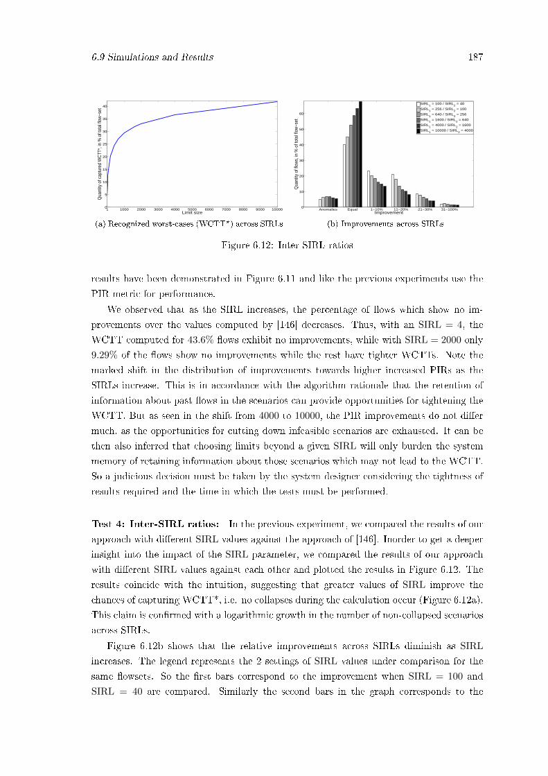
6.9 Simulations and Results 187
1 1000 2000 3000 4000 5000 6000 7000 8000 9000 100000
5
10
15
20
25
30
35
40
Limit size
Qua
ntity
of c
aptu
red
WC
TT*,
in %
of t
otal
flow
−set
(a) Recognized worst-cases (WCTT*) across SIRLs
Anomalies Equal 1−10% 11−20% 21−30% 31−100%0
10
20
30
40
50
60
Qua
ntity
of f
low
s, in
% o
f tot
al fl
ow−s
et
Improvement
SIRL1 = 100 / SIRL
2 = 40
SIRL1 = 256 / SIRL
2 = 100
SIRL1 = 640 / SIRL
2 = 256
SIRL1 = 1600 / SIRL
2 = 640
SIRL1 = 4000 / SIRL
2 = 1600
SIRL1 = 10000 / SIRL
2 = 4000
(b) Improvements across SIRLs
Figure 6.12: Inter-SIRL ratios
results have been demonstrated in Figure 6.11 and like the previous experiments use the
PIR metric for performance.
We observed that as the SIRL increases, the percentage of �ows which show no im-
provements over the values computed by [146] decreases. Thus, with an SIRL = 4, the
WCTT computed for 43.6% �ows exhibit no improvements, while with SIRL = 2000 only
9.29% of the �ows show no improvements while the rest have tighter WCTTs. Note the
marked shift in the distribution of improvements towards higher increased PIRs as the
SIRLs increase. This is in accordance with the algorithm rationale that the retention of
information about past �ows in the scenarios can provide opportunities for tightening the
WCTT. But as seen in the shift from 4000 to 10000, the PIR improvements do not di�er
much, as the opportunities for cutting down infeasible scenarios are exhausted. It can be
then also inferred that choosing limits beyond a given SIRL will only burden the system
memory of retaining information about those scenarios which may not lead to the WCTT.
So a judicious decision must be taken by the system designer considering the tightness of
results required and the time in which the tests must be performed.
Test 4: Inter-SIRL ratios: In the previous experiment, we compared the results of our
approach with di�erent SIRL values against the approach of [146]. Inorder to get a deeper
insight into the impact of the SIRL parameter, we compared the results of our approach
with di�erent SIRL values against each other and plotted the results in Figure 6.12. The
results coincide with the intuition, suggesting that greater values of SIRL improve the
chances of capturing WCTT*, i.e. no collapses during the calculation occur (Figure 6.12a).
This claim is con�rmed with a logarithmic growth in the number of non-collapsed scenarios
across SIRLs.
Figure 6.12b shows that the relative improvements across SIRLs diminish as SIRL
increases. The legend represents the 2 settings of SIRL values under comparison for the
same �owsets. So the �rst bars correspond to the improvement when SIRL = 100 and
SIRL = 40 are compared. Similarly the second bars in the graph corresponds to the

188 NoC Contention Analysis of Many Core Systems
improvement when SIRL = 256 and SIRL = 100 are compared. The X axis corresponds to
the percentage of improvement across bands, with equal meaning no improvement across
bands. Similarly, the Y axis re�ects the percentage of the �ows in the �ow set for which
the corresponding improvements were observed.
As seen in the �gure, our method with SIRL = 100 shows improvement against the same
method with SIRL = 40 in 60% of the cases (the �rst bar in the �equal� heading depicts that
40% �ows did not bene�t from increasing the SIRL value meaning there is improvement
in the rest of the cases, except for the anomalies), while the improvement is reported
only in 30% of the cases when comparing results of SIRL = 10000 and SIRL = 4000.
Thus, the number of scenarios with no improvement increases with SIRL. Conversely,
the number of scenarios with improvements decreases with SIRL across all improvement
ranges, suggesting that it may not be essential to perform the analysis with very high values
of SIRL beyond a certain value. The bene�ts of analyzing with higher SIRL diminish as
SIRL increases (especially for scenarios comprising of single-occurring �ows for which no
further scope of improvement is possible).
As already stated, the value of the SIRL in�uences the frequency of scenario collapses.
However, one interesting observation is the fact that higher SIRL does not necessarily
always lead to a tighter WCTT upper-bound. We explain this with a following example.
Consider the �ow f in the example depicted by Figure 6.9. Let us assume that fc and fdare potential candidates for pruning. Now, assume that greater SIRL performs a collapse
between occurrences of fa and fb. As the history information is lost, the �ows fc and fdwill contribute to the delays of both the �ows, fa and fb. On the other hand, a smaller
SIRL might trigger a collapse before (and after) the appearance of both fa and fb. In
this case, it may successfully prune one appearance of fc and fd, thereby resulting in the
situation (which we refer to an �anomaly�) where a smaller value of SIRL returns a tighter
WCTT estimate. As is visible from the results, the number of anomalies never exceeds
more than 8% in all the considered cases.
6.9.2 Trade o� between the approaches
: The above study also brings a very important result. If the network is not loaded and
the number of blockings experienced by a �ow (inclusive of direct and indirect blockings)
is low then the earlier recursive approaches as in [146] should be used as they will compute
the same WCTT as computed by the proposed approach in shorter time. But for a more
loaded network and for applications in which tighter WCTT estimates are required, the
branch and prune method proposed here can be employed.
We believe that in order to harness the capacity of the many-core system e�ciently,
most cores will be assigned tasks. This will lead to an increased contention on the network
as a result of the direct or indirect blockings and therefore for such a setup our method
is highly preferable. Although the use of the approach in [146] will lead to safe WCTT

6.9 Simulations and Results 189
estimates, it is overly pessimistic and therefore will lead to over-dimensioning of resources
and lower system utilization.
R2 R1 R3
R4
R5 R6 R7
R8
R9 R10 R11 R12
R13 R14 R15
R16
fA fB fC fD
fE fF fG fH
fI
Figure 6.13: Example Flow Set in a portion of the grid
6.9.3 Case Study with a speci�c �ow-set
Figure 6.13 shows one of the �ow-sets analyzed over a 4*4 grid that we shall use to demon-
strate some interesting properties. Additional details like the core and cache engine were
omitted to make the �gure simpler. In the rest of the document, we drop the pre�x f
and directly refer to the �ow by its alphabetical name. In this �ow set, we analyzed the
�ow A which originates in router R1 and terminates at the core associated with router
R16. B,C,D,E, F,G,H and I are the other �ows which also terminate at node R16. In
this example, in the worst-case scenario, every �ow can be potentially blocked by �ow I
(originating at R12) which is closest to the destination, then by �ow H and so on. To
provide a fair comparison with the approach in [146], we consider that every �ow is by
nature unregulated and non-blocking. By non-blocking we mean that the �ow next packet
can be sent without waiting for the acknowledgement of the previous packet. By applying
the approach in [146] or using our approach without any optimizations, one of the scenarios
which resulted in the WCTT for �ow A was:
{IHIEIDIHIEICIHIEIDIHIEIBIHIEIDIHIEICIHIEIDIHIEIA}. This scenario is a mani-
festation of the �task-level� and �network level� pessimism and exempli�es the case of an
over-estimated WCTT when infeasible blockings are not curtailed. Flows I and H are
positioned in a manner which enables them to frequently block the other �ows. This sce-
nario also presents a useful example for exploring the delay on the WCTT of �ow A if the
task-pro�les and task parameters of the blocking �ows are varied.

190 NoC Contention Analysis of Many Core Systems
6.9.4 Impact of Varying Packet Arrival Rates
0
5
10
15
20
25
0 10 20 30 40 50 60 70 80 90
Blo
ckin
g flo
w o
ccure
nce
s
MITR in microseconds
(a) No. of blockings by �ow I vs. itsMinInterRel(I)
90 100 110 120 130 140 150 160 170 180 190
0 10 20 30 40 50 60 70 80 90
WC
TT
in m
icro
seco
nds
MITR in microseconds
UnoptimizedOptimized
(b) WCTT of �ow A vs. Packet Arrival rate of �owI
Figure 6.14: WCTT of �ow A decreases with increase in MIA time of �ow I
The �ows originating closer to the destination of the analyzed �ow A in Figure 6.13
have a higher tendency to block it (�ow A) directly and indirectly (by blocking the other
�ows which are also in the path). To verify this, we tuned the MinInterRel() (MITR in
the �gure) of �ow I, increased it steadily and carried out the experiment, while keeping
the nature of the other parameters constant. Figure 6.14a shows that as MinInterRel(I)
increases, the number of times it can block the other �ows is invalidated and thus the
WCTT of �ow A decreases as expected as seen in Figure 6.14b. In contrast, since the
approach in [146] does not take into account the task characteristics, it allows these invalid
blockings to progress and as a result, irrespective of the change in the �ow parameters, the
computed WCTT remains constant (see solid line in Figure 6.14b).
6.9.5 Impact of Varying Task Patterns
The WCTT of a packet of a given �ow is also a�ected by the packet release pro�les of the
other �ows. To study this e�ect, we conducted the following tests in which we analyzed
the WCTT of �ow A (in Figure 6.13) by changing the packet pro�les of the blocking �ows.
In addition to the unregulated non-blocking pro�le assumed for all the �ows in [146], we
de�ned three packet pro�les S1, S2 and S3 (where S stands for Sparse) by generating syn-
thetic pattern arrivals and computing the MaxPcktRel(f, t) for each of these pro�les using
the method proposed in [91]. Figure 6.15 depicts the pro�les, in which the X-axis repre-
sents the time-line (in nanoseconds) and the Y-axis shows an upper bound on the number
of packets that can be generated in time t. The default pro�le, shown in Figure 6.15b,
models the unregulated non-blocking pro�le. Figure 6.16 summarizes the results of di�er-
ent tests carried by varying the parameters of the blocking �ows. The Y-axis represents
the computed values of the WCTT of �ow A. The X-axis contains the test name and
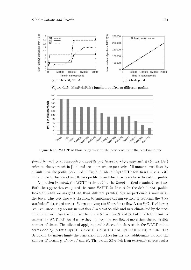
6.9 Simulations and Results 191
0
2
4
6
8
10
12
14
16
18
0 50000 100000 150000 200000Max
num
ber
of p
acke
ts: M
PR
F(f
,t)
Time in nanoseconds
S1S2S3
(a) Pro�les S1, S2, S3
0
50000
100000
150000
200000
250000
0 50000 100000 150000 200000Max
num
ber
of p
acke
ts: M
PR
F(f
,t)
Time in nanoseconds
Default profile
(b) Default pro�le
Figure 6.15: MaxPcktRel() function applied to di�erent pro�les
0
20
40
60
80
100
120
140
160
180
200
WCT
T in
mic
rose
cond
s
Figure 6.16: WCTT of Flow A by varying the �ow pro�les of the blocking �ows
should be read as < approach >< profile >< flows >, where approach ∈ {Unopt,Opt}refers to the approach in [146] and our approach, respectively. All unmentioned �ows by
default have the pro�le presented in Figure 6.15b. So OptS2IH refers to a test case with
our approach, the �ows I and H have pro�le S2 and the other �ows have the default pro�le.
As previously noted, the WCTT estimated by the Unopt method remained constant.
Both the approaches computed the same WCTT for �ow A for the default task pro�le.
However, when we assigned the �ows di�erent pro�les, Opt outperformed Unopt in all
the tests. This test case was designed to emphasize the importance of reducing the �task
pessimism� described earlier. When applying the S1 pro�le to �ow I, the WCTT of �ow A
reduced, since many occurrences of �ow I were not feasible and were eliminated by the tests
in our approach. We then applied the pro�le S1 to �ows H and D, but this did not further
impact the WCTT of �ow A since they did not intercept �ow A more than the admissible
number of times. The e�ects of applying pro�le S1 can be observed in the WCTT values
corresponding to tests OptS1I, OptS1IH, OptS1IHD and OptS1All in Figure 6.16. The
S2 pro�le, by nature limits the generation of packets further and additionally reduced the
number of blockings of �ows I and H. The pro�le S3 which is an extremely sparse packet

192 NoC Contention Analysis of Many Core Systems
pro�le, caused a major impact by drastically reducing the number of blockings and the
resulting WCTT decreased further. The e�ects of applying pro�le S3 can be observed in
the WCTT values corresponding to tests OptS3I, OptS3IH, OptS3IHD and OptS3All in
Figure 6.16.
6.9.6 Comparison with Related work
The proposed approach considers the impact due to direct and indirect blockings as in [147].
Unlike the works proposed by [135], [136], [137] or [138], it does not need any hardware
support for predictability, which is commonly not present in existing platforms. Conversely
our approach can be applied to a wider range of commercially available platforms. Fur-
thermore, the proposed approach does not incur the delay of �ushing out the preempted
�its as done by pre-emption based techniques [151]. We make no assumptions on the state
of the bu�ers as in Rehmati et.al [145] and do not restrict the model to �ows generat-
ing periodically arriving packets only. Due to the MaxPcktRel(f, t) function, even �ows
which generate packets randomly can be captured and thus our analysis is not restricted
to a�ne-arrival curves as in [142]. Through experiments we have demonstrated that our
approach computes tighter bounds when compared with the approach of [146], which as-
sumes a model that is closely related to ours. Additionally, the idea of retaining the history
information of �ows to prune further infeasible �ows lends novelty to our approach and
the concept of having SIRL as a tunable parameter makes the approach �exible.
6.10 Conclusions
In this chapter, we highlighted the problem of contention in a NoC as used in many-core
architectures. We proposed a solution to compute the worst-case traversal time of a packet
for such NoCs. This solution uses a branch and prune approach (BP) which improves on
the work presented in [146] by leveraging the task characteristics and thereby provides
tighter estimates on the computed WCTT. Inorder to tackle the complexity issues of BP
in corner cases, we extended it to a branch, prune and collapse method (BPC), which
via a con�gurable parameter provides a trade o� between the computation time/memory
usage and the WCTT tightness. A large set of experiments demonstrate the performance
of the proposed algorithms in comparison with the approach of [146]. In particular, our
work dominates their approach by yielding tighter WCTT estimates at the cost of extra
computation time, the e�ects of which can be mitigated by the optimized version i.e.
BPC. BPC on one hand limits the computational complexity, while on the other hand
still provides the bene�ts of tighter WCTT bounds. Future work will focus on identifying
the hot-spots in the network where a concentrated analysis e�ort promises substantial
tightening of the results by our method. This work can be extended to identify safe criteria
for dropping scenarios which provably do not contribute to theWCTT, or abstracting those,
which do not promise substantial improvements in the results.

Chapter 7
Thesis Summary, Re�ections and
Future Work
Once you have traveled, the voyage never ends,
but is played out over and over again in the
quietest chambers. The mind can never break o�
from the journey.
Pat Conroy
Real-time embedded system designers in many arenas are constantly facing competitive
pressure to provide more application features and improve performance capabilities. As
a result, it has become critical to master the ability to scale solutions and add features
within embedded form factors without dramatically a�ecting energy variables such as power
consumption and thermal output. Multicore systems have addressed these challenges by
o�ering higher computing performance, reduced chip count and lower costs, with reduced
power consumption. But multicore systems have yet to be certi�ed and validated for their
predictability, which features as an uncompromisable requirement for real-time systems.
The major challenge has been the presence of shared hardware resources like the memory
bus which poses a major hurdle to the timing analyzability of these systems. The aim
of this thesis was to formulate new solutions and design methodologies which are clearly
193

194 Thesis Summary, Re�ections and Future Work
required to analyze the impact of these shared resources. In this chapter we will summarize
the work done and present the open areas of this research.
7.1 Summary of the work
7.1.1 Analysis of the impact of the shared bus in multicores
Task 1 Task 2 Task 3 Task 4
External Interference incurred by Task i
Core 1
Per Task Cache Analysis
Per Task memory request profile
Per Core Interference Analysis
Per-Core memory request profile
time
Max
req
ues
ts
time
Max
req
ues
ts
time Max
req
ues
ts
time Max
req
ues
ts
Core 2 Core 3
Task i
Shared Memory Bus
Requests from core 1
Requests from core 2
Requests from Task i on core 3
time Max
req
ue
sts
time Max
req
ue
sts
Interference
Figure 7.1: Di�erent stages in the analysis
In this work, we followed a bottom up approach in computing the increased execution
time that a task may incur, when contending for the shared bus. On the basis of the
cache analysis of the tasks, we proposed two algorithms for deriving the per-task memory
request pro�le and per-core memory request pro�le as illustrated in Figure 7.1 and discussed

7.1 Summary of the work 195
in Chapter 3. Both the methods employed an interval splitting technique to reduce the
search space (of job arrivals) that had to be investigated to arrive at the combination
that can generate the maximum number of requests in a given time interval. It has been
demonstrated that the bounds obtained for per-task pro�les and per-core pro�les are tighter
than the existing state of the art. Also we believe that the problem of deriving the per-
core interference has been dealt with in an elegant manner by using the interval splitting
technique and transforming it to a knapsack problem, which is a novel solution to this
approach.
TDM arbiter Other arbiters
Compute Tmin(), Tmax() To model bus availability
Fixed priority arbiter
Compute worst-case delay for a Sequence of requests
Algorithm to compute worst-case assignment of requests to slots to
obtain max delay
Arbiter dependent stages
Arbiter independent stages
Work conserving arbiter
Tighten analysis by using sampling regions
Figure 7.2: Stages of development of the uni�ed framework
The tools developed in the earlier part of the work were critical in the development of
a uni�ed framework for analysis which we described in Chapter 4. They were instrumental
in modeling the availability of the bus to a given task, given di�erent arbitration models.
The di�erent stages of developing such a framework are described in Figure 7.2. The bus
availability model facilitated the identi�cation of potential free slots on the bus which the
analyzed task could utilize. Considering that the exact arrival pattern of requests cannot
be determined at design time, an algorithm was proposed to perform a request to free bus

196 Thesis Summary, Re�ections and Future Work
slot mapping with the aim of maximizing the execution time of the analyzed task, due to
the delay incurred on the shared bus. It was further shown that bounds can be tightened
by dividing the task into sampling regions and analyzing the delay incurred in each of
the regions. The highlight of the method was that it provided a general interface into
which di�erent arbiters can be seamlessly plugged to compute the resulting WCET of the
tasks. We also demonstrated the applicability of our framework for two di�erent arbiters:
a non-work-conserving TDM arbiter and work-conserving �xed-priority arbiter.
7.1.2 Analysis of PCM based multi-core systems
In Chapter 5, we explored a multicore system in which Phase Change Memory (PCM)
forms the main memory. As described earlier, what makes it di�erent from the popular
DRAM in terms of analysis is the wide di�erence in the time for completion of read and
write operations. For such a system, researchers have proposed memory controller schedul-
ing mechanisms to minimize core stall times, especially in the case of a time consuming
write operation. Given such a controller and request scheduling mechanism, a method to
compute the increase in the worst-case execution time of a task considering the contention
on this shared memory was presented. The proposed method takes into consideration the
di�erent read and write latencies of the PCM controller, the priorities of the tasks, the re-
quest scheduling of the controller, and the interference arising from the co-executing tasks.
The analysis was carried out in two main phases. In the �rst phase, the busy and the idle
periods of the bus with respect to the analyzed task were determined. In the second phase,
the requests were scheduled in the available idle periods of the bus, with the objective to
maximize the overall execution time of the analyzed task. This work is important since it is
the �rst analysis in this �eld, since previous works did not consider modeling the memory
controller scheduling and assumed a constant access time for read and write accesses.
7.1.3 Analyzing the contention delay of a packet in many-core systems
Given that the shared bus architecture does not scale beyond a limited number of cores,
�many-core� systems based on the NoC architecture have emerged. Chapter 6 highlights
the problems of employing these systems for real-time applications and proposes a method
to compute an upper bound on the traversal time of a packet when routed over the network

7.2 Limitations of current work and future directions 197
(on the chip) to its destination. The drawbacks of the existing approaches were highlighted
�rst and then were overcome by modeling the �ow characteristics (like the minimum inter-
release time between packets) in the network and leveraging these vital characteristics
to derive tighter estimates. We proposed two main algorithms: the Branch and Prune
(BP) algorithm and the Branch, Prune and Collapse (BP) algorithm. The BP algorithm
provides a tight estimate by enumeration and early pruning of infeasible scenarios, but
can be computationally intensive for a heavily loaded network. To tackle this problem, we
propose the BPC algorithm that provides a tradeo� between complexity and tightness by
providing a con�gurable parameter to the system designer. Both these approaches were
validated by a set of experiments against the state of the art techniques and were shown
to provide tighter bounds.
7.2 Limitations of current work and future directions
7.2.1 Support for preemptive tasks
The current analysis is done under the assumption that tasks cannot be not preempted and
will run to completion. But this rules out an important category of real-time applications
in which tasks must be preemptible, and hence an analysis for such tasks is important.
Consider a multicore system in which every core has its private cache. In such a scenario,
a task which preempts a currently executing task may evict its cache lines. When the
preempted task resumes, it may have to re-fetch the evicted cache lines from memory
and thereby will incur an addition delay which is called Cache Related Preemption Delay
(CRPD). Methods to compute this delay have been explored for uniprocessors and must
be integrated in the current analysis.
This problem of computing the WCET, with such a model, is exacerbated in multicores,
considering that re-fetching the (analyzed) preempted tasks' evicted caches increases the
tra�c on the bus and increases the interference. Hence, the analysis gets complex as we
have a set of preemptible tasks on all cores and as a consequence computing the external
interference on the shared bus will need to factor in all possible combinations of tasks and
preemptions which is prohibitively expensive. To reduce the complexity of the analysis, a

198 Thesis Summary, Re�ections and Future Work
feasible approach called the limited-preemption model can be employed, in which preemp-
tions are allowed only at speci�cally marked points during a task execution. Such a model
provides for tighter bounds, besides reducing the complexity.
7.2.2 Timing Analysis of many core systems.
The many-core area o�ers a range of unexplored problems. In the work that we presented,
we assumed the presence of a single virtual channel. Some systems also allow the creation
of multiple channels by having multiple bu�ers at the input ports of each router. In a
scenario in which the �its of a packet are blocked due to congestion ahead, some other
packet may transmit their �its and save it into the alternative bu�ers. Some book-keeping
regarding which channels belong to each packet must be maintained, but the performance
of these systems is better since it facilitates higher network utilization.
Another interesting feature in many-core systems like Tilera is that they o�er the
possibility of clustering cores and restricting tra�c across cores using hardwalls. These
capabilities can be leveraged to group tasks of di�erent criticalities in various clusters and
reserve resources in a manner to satisfy their quality of service requirements.
Many core systems generally have a non-uniform memory access model in which the
memory controllers are placed on the periphery of the grid. Cores which are closer to
the controllers incur a lower latency in memory access. Analyzing the traversal time of
a packet between the core and the memory, given such a topology has it own challenges.
In the same vein, mapping tasks to cores to ensure that all packets are delivered to the
destination within pre-set deadlines is another interesting area of exploration.
7.2.3 DRAM and PCM hierarchy
The analysis carried out in this thesis is the �rst step in the analysis of memory systems
with asymmetric read and write latencies and had a strong assumption that considered
PCM as the main memory. But a more practical o�-chip hierarchy is when PCM comple-
ments DRAM as the main memory. When data is not found in the cache, the DRAM is
�rst consulted and then the PCM memory is consulted. This analysis will have its own
challenges and will have to consider the scheduling of requests at the DRAM memory
controller and the PCM memory controller.

7.2 Limitations of current work and future directions 199
7.2.4 WCET analysis in identical and heterogeneous multicores
Identical multicores which have the same ISA (instruction set architecture) but with asym-
metric cores w.r.t performance, comprising of both simple and complex cores, have recently
been proposed to cater to the quality of service requirements of di�erent tasks. The pro-
cessors in an asymmetric multi-core architecture share the same ISA but their micro-
architectures (pipeline and caches) are very di�erent. For example, ARM has recently an-
nounced big.LITTLE processing for mobile platforms where high-performance, out-of-order
(bigger) Cortex A-15 cores with a 15-stage pipeline are integrated with energy-e�cient,
in-order (smaller) Cortex A-7 cores, armed with a 8 stage pipeline in the same chip. The
execution time will correspondingly be di�erent, depending on the processors on which the
task is assigned. Additionally if the cores share the same hardware resources, then the de-
lay due to contention has to be factored in the overall execution time of the task. The same
is true for heterogeneous multicores in which the cores are speci�cally designed to handle
special functions and therefore di�er in their ISA as well as clock speeds �Examples of such
systems are the GPGPU's from NVidia and OMAP processors from Texas Instruments.
Analyzing the execution time of tasks in such systems is another unexplored area.
7.2.5 WCET and parallelization
The parallelization of software poses a number of di�culties, particularly when deriving its
WCET for an application. A fundamental di�erence when software is executed in parallel
is the need for the communication between di�erent cores, either to exchange data to be
processed and to perform synchronization to ensure that the �nal results are consistent.
Even an operation as straightforward as writing a value into a shared variable and then
reading it back involves some communication if the components reading and writing are
executed on di�erent cores. These e�ects must be factored in the eventual analysis.
7.2.6 End Notes
Although intelligent software based techniques can alleviate the existing challenges in em-
ploying multicores for real-time systems, it will take an equal e�ort from the industry to
help build more predictable systems as well. Additionally, it holds for all system designers,
that the true bene�ts of multicores can be leveraged only by studying their architecture
200 Thesis Summary, Re�ections and Future Work
and understanding the causes of average-case performance degradation, and then designing
applications accordingly to e�ciently harness the inherent parallelism. Real-time system
designers in particular, need to be able to analyze the worst-case degradation that an ap-
plication may su�er in the context of their temporal behaviour. The results from the work
done so far has been a strong motivator to strive towards the ultimate aim of contribut-
ing towards building a stronger timing analysis tool and this thesis has been an endeavor
towards that aim.
Bibliography
[1] T. D. Morton, Embedded Microcontrollers. Prentice Hall Publishers, 2001.
[2] J. Hale, �Smarter sensor processing for UAS payloads.�
http://mil-embedded.com/articles/smarter-sensor-processing-uas-payloads/.
[3] P. Koopman, �Embedded system design issues (the rest of the story),� in Proceedings
of the 1996 International Conference on Computer Design, VLSI in Computers and
Processors, ICCD '96, pp. 310�, IEEE Computer Society, 1996.
[4] S. Baruah and J. Goossens, Scheduling Real-time Tasks: Algorithms and Complexity,
2003.
[5] D. Isovic and G. Fohler, �E�cient scheduling of sporadic, aperiodic, and periodic
tasks with complex constraints,� in Real-Time Systems Symposium, 2000. Proceed-
ings. The 21st IEEE, pp. 207 �216, 2000.
[6] R. Mall, Real-Time Systems: Theory and Practice. Pearson Power, 2007.
[7] S. K. Baruah, �The non-preemptive scheduling of periodic tasks upon multiproces-
sors,� Real-Time Syst., vol. 32, pp. 9�20, Feb. 2006.
[8] B. Akesson, A. Molnos, A. Hansson, J. Ambrose Angelo, and K. Goossens, �Com-
posability and predictability for independent application development, veri�cation,
and execution,� in Multiprocessor System-on-Chip: Hardware Design and Tool In-
tegration (M. Hübner and J. Becker, eds.), pp. 25�56, Springer Verlag, November
2010.
201

202 BIBLIOGRAPHY
[9] C. Berg, J. Engblom, and R. Wilhelm, �Requirements for and design of a processor
with predictable timing,� in Perspectives Workshop: Design of Systems with Pre-
dictable Behaviour, 16.-19. November 2003, volume 03471 of Dagstuhl Seminar Pro-
ceedings. IBFI, Schloss Dagstuhl, 2004.
[10] R. Wilhelm, J. Engblom, A. Ermedahl, N. Holsti, S. Thesing, D. Whalley, G. Bernat,
C. Ferdinand, R. Heckmann, T. Mitra, F. Mueller, I. Puaut, P. Puschner, J. Staschu-
lat, and P. Stenström, �The worst-case execution-time problem � overview of methods
and survey of tools,� ACM Trans. Embed. Comput. Syst., vol. 7, pp. 36:1�36:53, 2008.
[11] H. Kopetz, �An integrated architecture for dependable embedded systems,� in Pro-
ceedings of the 23rd IEEE International Symposium on Reliable Distributed Systems,
SRDS '04, pp. 160�161, IEEE Computer Society, 2004.
[12] S. Chakraborty, M. Lukasiewycz, C. Buckl, S. Fahmy, N. Chang, S. Park, Y. Kim,
P. Leteinturier, and H. Adlkofer, �Embedded systems and software challenges in elec-
tric vehicles,� in Design, Automation Test in Europe Conference Exhibition (DATE),
2012, pp. 424�429, 2012.
[13] J. Ramsey, �Integrated Modular Avionics: Less is More,� 2007.
http://www.aviationtoday.com/av/commercial/Integrated-Modular-Avionics-Less-
is-More_8420.html#.UoUIAI9lUak.
[14] V. Tran, D.-B. Liu, and B. Hummel, �Component-based systems development: chal-
lenges and lessons learned,� in Software Technology and Engineering Practice, 1997.
Proceedings., Eighth IEEE International Workshop on [incorporating Computer Aided
Software Engineering], pp. 452 �462, jul 1997.
[15] S. Keckler, O. Olukotun, and H. Hofstee, Multicore Processors and Systems. Inte-
grated Circuits and Systems, Springer London, Limited, 2009.
[16] R. I. Davis and A. Burns, �A survey of hard real-time scheduling for multiprocessor
systems,� ACM Comput. Surv., vol. 43, pp. 35:1�35:44, Oct. 2011.

BIBLIOGRAPHY 203
[17] L. Seiler, D. Carmean, E. Sprangle, T. Forsyth, M. Abrash, P. Dubey, S. Junkins,
A. Lake, J. Sugerman, R. Cavin, R. Espasa, E. Grochowski, T. Juan, and P. Han-
rahan, �Larrabee: a many-core x86 architecture for visual computing,� ACM Trans.
Graph., vol. 27, pp. 18:1�18:15, Aug. 2008.
[18] Techopedia, �Multicore,� 2006.
//http://www.techopedia.com/de�nition/5305/multicore.
[19] Intel Corporation, Intel 4 Series Chipset Family Datasheet, For the Intel 82Q45,
82Q43, 82B43, 82G45, 82G43, 82G41 Graphics and Memory Controller Hub
(GMCH) and the Intel R©82P45, 82P43 Memory Controller Hub (MCH), 2010.
[20] S. Zhuravlev, S. Blagodurov, and A. Fedorova, �Addressing shared resource con-
tention in multicore processors via scheduling,� SIGPLAN Not., vol. 45, no. 3,
pp. 129�142, 2010.
[21] D. Wentzla�, P. Gri�n, H. Ho�mann, L. Bao, B. Edwards, C. Ramey, M. Mattina,
C.-C. Miao, J. F. B. III, and A. Agarwal, �On-chip interconnection architecture of
the tile processor,� IEEE Micro, vol. 27, pp. 15�31, 2007.
[22] Kalray, �Kalray MPPA 256 .�
http://www.kalray.eu/products/mppa-manycore/mppa-256/.
[23] Intel, �Intel Xeon Phi Coprocessor .�
http://www-ssl.intel.com/content/dam/www/public/us/en/documents/datasheets/xeon-
phi-coprocessor-datasheet.pdf.
[24] Intel, �The single-chip-cloud computer,� 2010.
http://www.intel.com/content/dam/www/public/us/en/documents/technology-
briefs/intel-labs-single-chip-cloud-article.pdf.
[25] L. Benini and G. De Micheli, �Networks on chips: a new soc paradigm,� Computer,
vol. 35, pp. 70 �78, jan 2002.
[26] �Market Applications of Phase Change Memory (PCM).�
http://ovonyx.com/technology/market-applications-of-phase-change-memory-
pcm.html.
204 BIBLIOGRAPHY
[27] S. Mohan, M. Caccamo, L. Sha, R. Pellizzoni, G. Arundale, R. Kegley, and D. de Niz,
�Using multicore architectures in cyber-physical systems,� Workshop on Developing
Dependable and Secure Automotive Cyber-Physical Systems from Components., 2011.
[28] N. R. Storey, Safety Critical Computer Systems. Addison-Wesley Longman Publish-
ing Co., Inc., 1996.
[29] ISO26262-4, Road vehicles � Functional safety � Part 4: Product development at the
system level, 1 ed., 2011.
[30] IEC 61508, Functional safety of electrical/electronic/programmable electronic safety-
related systems, 2010.
[31] RECOMP, �Reduced Certi�cation Costs Using Trusted Multi-core Platforms .�
http://atcproyectos.ugr.es/recomp/.
[32] MERASA, �Multi-Core Execution of Hard Real-Time Applications Supporting
Analysability .�
http://ginkgo.informatik.uni-augsburg.de/merasa-web/.
[33] ARAMiS, �Automotive, Railway and Avionics multicore systems.�
http://www.projekt-aramis.de/index.php.
[34] C. E. Salloum, �A New Generation of Multi-Core Processors Designed for Safety-
Critical Embedded Systems .�
http://www.across-project.eu/.
[35] CESAR, �Cost-e�cient methods and processes for safety relevant embedded systems
.�
http://www.cesarproject.eu/index.php?id=6.
[36] J. Gustafsson and A. Ermedahl, �Experiences from applying wcet analysis in indus-
trial settings.,� in ISORC, pp. 382�392, IEEE Computer Society, 2007.
[37] Rapita Systems Ltd., �Rapitime explained.�
http://www.rapitasystems.com/downloads/rapitime_explained_white_paper".

BIBLIOGRAPHY 205
[38] P. Lokuciejewski and P. Marwedel, �Summary and future work,� in Worst-Case Exe-
cution Time Aware Compilation Techniques for Real-Time Systems, Embedded Sys-
tems, pp. 229�234, Springer Netherlands, 2011.
[39] C. Ferdinand, R. Heckmann, and B. Franzen, �Static memory and timing analysis
of embedded systems code,� in Proceedings of VVSS2007 - 3rd European Symposium
on Veri�cation and Validation of Software Systems, 23rd of March 2007, Eindhoven
(P. Groot, ed.), 2007.
[40] N. Holsti and S. Saarinen, �Status of the Bound-T WCET tool,� in 2nd International
Workshop on Worst-Case Execution Time Analysis (WCET'2002), 2002.
[41] X. Li, Y. Liang, T. Mitra, and A. Roychoudhury, �Chronos: A timing analyzer for
embedded software,� in Science of Computer Programming, 2007.
[42] �Heptane.�
http://www.irisa.fr/aces/work/heptane-demo/heptane.html.
[43] A. Ermedahl, A Modular Tool Architecture for Worst-Case ExecutionTime Analysis.
VDM Verlag, 2008.
[44] R. Kirner, P. Puschner, and I. Wenzel, �Measurement-based worst-case execution
time analysis using automatic test-data generation,� in Proc. 4th Euromicro Inter-
national Workshop on WCET Analysis, pp. 67�70, June 2004.
[45] �Bus Computing.�
http://en.wikipedia.org/wiki/Bus_(computing).
[46] �Bus and Bits.�
http://blog.teachbook.com.au/index.php/computer-science/1-0-hardware-
overview/bus-bits/.
[47] D. J. Sorin, M. D. Hill, and D. A. Wood, A Primer on Memory Consistency and
Cache Coherence. Morgan & Claypool Publishers, 1st ed., 2011.
[48] Optimizing Application Performance on Intel Core Microarchitecture Using
Hardware-Implemented Prefetchers.

206 BIBLIOGRAPHY
[49] T. Noergaard, Embedded Systems Architecture: A Comprehensive Guide for Engi-
neers and Programmers. Newnes, 2005.
[50] R. Wilhelm, D. Grund, J. Reineke, M. Schlickling, M. Pister, and C. Ferdinand,
�Memory hierarchies, pipelines, and buses for future architectures in time-critical
embedded systems,� IEEE Transactions on Computer-Aided Design of Integrated
Circuits and Systems, vol. 28, pp. 966�978, July 2009.
[51] J. Reineke, D. Grund, C. Berg, and R. Wilhelm, �Timing predictability of cache
replacement policies,� Real-Time Systems, vol. 37, pp. 99�122, Nov. 2007.
[52] C. Ferdinand and R. Wilhelm, �E�cient and precise cache behavior prediction for
real-time systems,� Real-Time Systems, vol. 17, pp. 131�181, 1999.
[53] T. King, �Cache partitioning increases CPU utilization for safety-critical multicore
applications.�
http://mil-embedded.com/articles/cache-utilization-safety-critical-multicore-
applications/#.
[54] JEDEC Solid State Technology Association, DDR3 SDRAM Speci�cation, JESD79-
3E ed., July 2010.
[55] B. Jacob, N. G. Spencer, and D. Wang, Memory Systems Cache, DRAM, Disk,
pp. 497�520. Morgan Kaufmann, 2007.
[56] S. Rixner, W. J. Dally, U. J. Kapasi, P. Mattson, and J. D. Owens, �Memory access
scheduling,� in ISCA '00: Proceedings of the 27th annual international symposium
on Computer architecture, pp. 128�138, 2000.
[57] B. Akesson and K. Goossens, �Architectures and modeling of predictable memory
controllers for improved system integration,� in Design, Automation Test in Europe
Conference Exhibition (DATE), 2011, pp. 1�6, 2011.
[58] M. Paolieri, E. Quinones, F. Cazorla, and M. Valero, �An Analyzable Memory Con-
troller for Hard Real-Time CMPs,� Embedded Systems Letters, IEEE, vol. 1, no. 4,
pp. 86 �90, 2009.
BIBLIOGRAPHY 207
[59] J. Reineke, I. Liu, H. Patel, S. Kim, and E. A. Lee, �PRET DRAM Controller: Bank
Privatization for Predictability and Temporal Isolation,� in CODES+ISSS '11: Pro-
ceedings of the IEEE/ACM international conference on Hardware/software codesign
and system synthesis, pp. 99�108, Oct. 2011.
[60] J. Dodd, �Adaptive page management,� July 2006. US Patent 7,076,617.
[61] S. Goossens, B. Akesson, and K. Goossens, �Conservative Open-page Policy for
Mixed Time-Criticality Memory Controllers,� in Proc. Design, Automation and Test
in Europe Conference and Exhibition (DATE), pp. 525�530, 2013.
[62] O. Mutlu and T. Moscibroda, �Parallelism-Aware Batch Scheduling: Enabling High-
Performance and Fair Shared Memory Controllers,� IEEE Micro, vol. 29, no. 1,
pp. 22�32, 2009.
[63] J. Shao and B. Davis, �A burst scheduling access reordering mechanism,� in Proceed-
ings of the 13th International Symposium on High-Performance Computer Architec-
ture, pp. 285�294, 2007.
[64] S. Heithecker and R. Ernst, �Tra�c shaping for an FPGA based SDRAM controller
with complex QoS requirements,� pp. 575�578, 2005.
[65] S. Whitty and R. Ernst, �A bandwidth optimized SDRAM controller for the MOR-
PHEUS recon�gurable architecture,� in Proceedings of the Parallel and Distributed
Processing Symposium (IPDPS), 2008.
[66] A. Burchard, E. Hekstra-Nowacka, and A. Chauhan, �A real-time streaming memory
controller,� pp. 20�25, 2005.
[67] C. Macian, S. Dharmapurikar, and J. Lockwood, �Beyond performance: Secure and
fair memory management for multiple systems on a chip,� in IEEE International
Conference on Field-Programmable Technology (FPT), pp. 348�351, 2003.
[68] W.-D. Weber, E�cient Shared DRAM Subsystems for SOCs. Sonics, Inc, 2001.
White paper.

208 BIBLIOGRAPHY
[69] K. Lee, T. Lin, and C. Jen, �An e�cient quality-aware memory controller for multi-
media platform SoC,� vol. 15, no. 5, pp. 620�633, 2005.
[70] S. Novak, J. Peck Jr, and S. Waldron, �Method and apparatus for optimizing memory
performance with opportunistic refreshing,� Nov. 2000. US Patent 6,147,921.
[71] S. Biswas, �Refresh-ahead and burst refresh preemption technique for managing dram
in computer system,� May 1999. US Patent 5,907,857.
[72] J. Rosen, A. Andrei, P. Eles, and Z. Peng, �Bus access optimization for predictable
implementation of real-time applications on multiprocessor systems-on-chip,� in
RTSS '07: Proceedings of the 28th IEEE International Real-Time Systems Sym-
posium, pp. 49�60, IEEE Computer Society, 2007.
[73] S. Chattopadhyay, A. Roychoudhury, and T. Mitra, �Modeling shared cache and bus
in multi-cores for timing analysis,� in Proceedings of the 13th International Workshop
on Software & Compilers for Embedded Systems, pp. 6:1�6:10, 2010.
[74] T. Kelter, H. Falk, P. Marwedel, S. Chattopadhyay, and A. Roychoudhury, �Bus-
Aware Multicore WCET Analysis through TDMA O�set Bounds,� in Proceedings of
the 2011 Euromicro Conference on Real-Time Systems, pp. 3 �12, 2011.
[75] A. Schranzhofer, J.-J. Chen, and L. Thiele, �Timing analysis for TDMA arbitration
in resource sharing systems,� in 16th IEEE Real-Time and Embedded Technology and
Applications Symposium, pp. 215�224, 2010.
[76] A. Schranzhofer, R. Pellizzoni, J.-J. Chen, L. Thiele, and M. Caccamo, �Timing
analysis for resource access interference on adaptive resource arbiters,� in Real-Time
and Embedded Technology and Applications Symposium, 2011.
[77] M. Lv, W. Yi, N. Guan, and G. Yu, �Combining abstract interpretation with model
checking for timing analysis of multicore software,� in Proceedings of the 2010 31st
IEEE Real-Time Systems Symposium, RTSS '10, pp. 339�349, 2010.
[78] A. Gustavsson, A. Ermedahl, B. Lisper, and P. Pettersson, �Towards WCET analysis
of multicore architectures using UPPAAL,� in WCET, pp. 101�112, 2010.

BIBLIOGRAPHY 209
[79] R. Pellizzoni, A. Schranzhofer, J.-J. Chen, M. Caccamo, and L. Thiele, �Worst case
delay analysis for memory interference in multicore systems,� in Conference on De-
sign, Automation and Test in Europe, pp. 741�746, 2010.
[80] S. Schliecker, M. Negrean, and R. Ernst, �Bounding the shared resource load for the
performance analysis of multiprocessor systems,� in Proceedings of the Conference
on Design, Automation and Test in Europe, pp. 759�764, 2010.
[81] M. A. Marsan, G. Balbo, G. Conte, and F. Gregoretti, �Modeling bus contention and
memory interference in a multiprocessor system,� IEEE Trans. Comput., vol. 32,
no. 1, pp. 60�72, 1983.
[82] M. Paolieri, E. Qui nones, F. J. Cazorla, G. Bernat, and M. Valero, �Hardware sup-
port for wcet analysis of hard real-time multicore systems,� in ISCA '09: Proceedings
of the 36th annual international symposium on Computer architecture, pp. 57�68,
ACM, 2009.
[83] J. Yan and W. Zhang, �WCET analysis for multi-core processors with shared L2
instruction caches,� in RTAS '08: Proceedings of the 2008 IEEE Real-Time and
Embedded Technology and Applications Symposium, pp. 80�89, 2008.
[84] Y. Ding and W. Zhang, �Static analysis of worst-case inter-core communication la-
tency in cmps with 2d-mesh noc,� in Proceedings of the 2012 WiP session of LCTES,
2012.
[85] Y. Li, V. Suhendra, Y. Liang, T. Mitra, and A. Roychoudhury, �Timing analysis of
concurrent programs running on shared cache multi-cores,� in Real-Time Systems
Symposium, 2009, RTSS 2009. 30th IEEE, pp. 57 �67, dec. 2009.
[86] V. Suhendra and T. Mitra, �Exploring locking & partitioning for predictable shared
caches on multi-cores,� in DAC '08: Proceedings of the 45th annual Design Automa-
tion Conference, pp. 300�303, ACM, 2008.
[87] N. Guan, M. Stigge, W. Yi, and G. Yu, �Cache-aware scheduling and analysis for
multicores,� in Proceedings of the seventh ACM international conference on Embedded
software, pp. 245�254, 2009.

210 BIBLIOGRAPHY
[88] G. Taylor, P. Davies, and M. Farmwald, �The tlb slice�a low-cost high-speed address
translation mechanism,� in ISCA '90: Proceedings of the 17th annual international
symposium on Computer Architecture, pp. 355�363, ACM, 1990.
[89] D. Hardy, T. Piquet, and I. Puaut, �Using bypass to tighten WCET estimates for
multi-core processors with shared instruction caches,� in Proceedings of the 2009 30th
IEEE Real-Time Systems Symposium, pp. 68�77, 2009.
[90] J. Rosén, A. Andrei, P. Eles, and Z. Peng, �Bus access optimization for predictable
implementation of real-time applications on multiprocessor systems-on-chip,� in Pro-
ceedings of the Real-Time Systems Symposium, pp. 49�60, 2007.
[91] D. Dasari, B. Andersson, V. Nelis, S. M. Petters, A. Easwaran, and J. Lee, �Response
time analysis of COTS-based multicores considering the contention on the shared
memory bus,� in IEEE 10th International Conference on Trust, Security and Privacy
in Computing and Communications, pp. 1068�1075, nov. 2011.
[92] R. J. Bril, J. J. Lukkien, and W. F. Verhaegh, �Worst-case response time analysis of
real-time tasks under �xed-priority scheduling with deferred preemption,� Real-Time
Systems, vol. 42, pp. 63�119, August 2009.
[93] K. Tindell, A. Burns, and A. Wellings, �Calculating controller area network (can)
message response times,� Control Engineering Practice, vol. 3, no. 8, pp. 1163�1169,
1995.
[94] B. Sprunt, �The basics of performance-monitoring hardware,� IEEE Micro, vol. 22,
no. 4, pp. 64�71, 2002.
[95] K. W. Tindell, A. Burns, and A. J. Wellings, �An extendible approach for analyzing
�xed priority hard real-time tasks,� Real-Time Systems, vol. 6, pp. 133�151, March
1994.
[96] A. V. Goldberg and A. Marchetti-Spaccamela, �On �nding the exact solution of a
zero-one knapsack problem,� in Proceedings of the sixteenth annual ACM symposium
on Theory of computing, STOC '84, pp. 359�368, ACM, 1984.
BIBLIOGRAPHY 211
[97] T. H. Cormen, C. E. Leiserson, R. L. Rivest, and C. Stein, Introduction to Algorithms,
2nd Ed. McGraw-Hill, 2001.
[98] J. Carpenter, S. Funk, P. Holman, A. Srinivasan, J. Anderson, and S. Baruah, A Cat-
egorization of Real-time Multiprocessor Scheduling Problems and Algorithms, ch. 30.
Chapman & Hall/CRC, 2004.
[99] C. L. Liu and J. W. Layland, �Scheduling algorithms for multiprogramming in a
hard-real-time environment,� J. ACM, vol. 20, pp. 46�61, Jan. 1973.
[100] J. Goossens and R. Devillers, �The non-optimality of the monotonic priority assign-
ments for hard real-time o�set free systems,� Real-Time Systems, vol. 13, pp. 107�
126, 1997.
[101] M. Zhou, S. Bock, A. Ferreira, B. Childers, R. Melhem, and D. Mosse, �Real-time
scheduling for phase change main memory systems,� in TrustCom, ICESS11, pp. 991
�998, nov. 2011.
[102] H. Shah, A. Raabe, and A. Knoll, �Priority division: A high-speed shared-memory
bus arbitration with bounded latency,� in Design, Automation Test in Europe Con-
ference Exhibition (DATE), 2011, pp. 1 �4, march 2011.
[103] S. Raoux, G. W. Burr, M. J. Breitwisch, C. T. Rettner, Y.-C. Chen, R. M. Shelby,
M. Salinga, D. Krebs, S.-H. Chen, H.-L. Lung, and C. H. Lam, �Phase-change random
access memory: A scalable technology,� IBM Journal of Research and Development,
vol. 52, pp. 465 �479, july 2008.
[104] A. P. Ferreira, B. R. Childers, R. G. Melhem, D. Mossé, and M. Yousif, �Using pcm
in next-generation embedded space applications,� in IEEE Real-Time and Embedded
Technology and Applications Symposium, pp. 153�162, 2010.
[105] B. C. Lee, E. Ipek, O. Mutlu, and D. Burger, �Architecting phase change memory as a
scalable dram alternative,� in Proceedings of the 36th annual international symposium
on Computer architecture, ISCA '09, pp. 2�13, ACM, 2009.

212 BIBLIOGRAPHY
[106] S. Schliecker and R. Ernst, �Real-time performance analysis of multiprocessor systems
with shared memory,� ACM Transactions in Embedded Computing Systems, vol. 10,
pp. 22:1�22:27, 2011.
[107] Y. Hara, H. Tomiyama, S. Honda, H. Takada, and K. Ishii, �Chstone: A benchmark
program suite for practical c-based high-level synthesis,� in ISCAS, pp. 1192�1195,
2008.
[108] VxWorks Applications Programmers Guide, 6.8.
[109] Intel Corp., Intel 64 and IA-32 Architecture Software Developers Manual Volume 3B:
System Programming Guide, Part 2.
[110] M. R. Guthaus, J. S. Ringenberg, D. Ernst, T. M. Austin, T. Mudge, and R. B.
Brown, �Mibench: A free, commercially representative embedded benchmark suite,�
in WWC '01: Proceedings of the Workload Characterization, 2001. WWC-4. 2001
IEEE International Workshop, pp. 3�14, IEEE Computer Society, 2001.
[111] J. Gustafsson, A. Betts, A. Ermedahl, and B. Lisper, �The Mälardalen WCET bench-
marks � past, present and future,� pp. 137�147, OCG, July 2010.
[112] B. Akesson, A. Hansson, and K. Goossens, �Composable resource sharing based on
latency-rate servers,� in Digital System Design, Architectures, Methods and Tools,
2009. DSD'09. 12th Euromicro Conference on, pp. 547�555, IEEE, Aug. 2009.
[113] H. Shah, A. Raabe, and A. Knoll, �Bounding wcet of applications using sdram with
priority based budget scheduling in mpsocs,� in Design, Automation Test in Europe
Conference Exhibition (DATE), 2012, pp. 665�670, 2012.
[114] Z. P. Wu, Y. Krish, and R. Pellizzoni, �Worst case analysis of dram latency in multi-
requestor systems,� in Proc. of IEEE Real-Time Systems Symposium, 2013.
[115] H. Yun, G. Yao, R. Pellizzoni, M. Caccamo, and L. Sha, �Memory access control in
multiprocessor for real-time systems with mixed criticality,� in Real-Time Systems
(ECRTS), 2012 24th Euromicro Conference on, pp. 299�308, 2012.

BIBLIOGRAPHY 213
[116] M. Behnam, R. Inam, T. Nolte, and M. Sjodin, �Multi-core composability in the face
of memory-bus contention,� in Proceedings of the 5th Workshop on Compositional
Theory and Technology for Real-Time Embedded Systems (CRTS), 2012.
[117] D. Dasari and V. Nelis, �An analysis of the impact of bus contention on the wcet
in multicores,� in IEEE 9th International Conference on Embedded Software and
Systems (HPCC-ICESS), pp. 1450 �1457, june 2012.
[118] T. Austin, E. Larson, and D. Ernst, �SimpleScalar: An infrastructure for computer
system modeling,� Computer, vol. 35, no. 2, pp. 59�67, 2002.
[119] JEDEC Solid State Technology Association, DDR3 SDRAM Speci�cation, JESD79-
3F ed., 2012.
[120] �Phase Change Memory: Altered states.�
http://www.economist.com/node/21560981.
[121] J. Handy, �Phase Change Memory will Change Memory System Design.�
http://www.rtcmagazine.com/articles/view/101556.
[122] �Phase Change Memory.�
http://www.pdl.cmu.edu/SDI/2009/slides/Numonyx.pdf.
[123] C. Lee, M. Potkonjak, and W. Mangione-Smith, �Mediabench: a tool for evaluat-
ing and synthesizing multimedia and communications systems,� in Microarchitec-
ture, 1997. Proceedings., Thirtieth Annual IEEE/ACM International Symposium on,
pp. 330 �335, dec 1997.
[124] B. C. Lee, E. Ipek, O. Mutlu, and D. Burger, �Architecting phase change memory as
a scalable dram alternative,� in ISCA '09, pp. 2�13, ACM, 2009.
[125] M. K. Qureshi, V. Srinivasan, and J. A. Rivers, �Scalable high performance main
memory system using phase-change memory technology,� ISCA '09.
[126] A. P. Ferreira, B. Childers, R. Melhem, D. Mosse, and M. Yousif, �Using PCM
in next-generation embedded space applications,� in RTAS '10, IEEE Computer
Society, 2010.
214 BIBLIOGRAPHY
[127] P. Zhou, B. Zhao, J. Yang, and Y. Zhang, �A durable and energy e�cient main
memory using phase change memory technology,� in ISCA '09, pp. 14�23, ACM,
2009.
[128] W. Zhang and T. Li, �Exploring phase change memory and 3d die-stacking for
power/thermal friendly, fast and durable memory architectures,� in PACT '09,
pp. 101�112, 2009.
[129] M. K. Qureshi, M. Franceschini, and L. A. Lastras-Montaño, �Improving read per-
formance of phase change memories via write cancellation and write pausing,� in
HPCA, pp. 1�11, 2010.
[130] P. S. Magnusson, M. Christensson, J. Eskilson, D. Forsgren, G. Hållberg, J. Högberg,
F. Larsson, A. Moestedt, and B. Werner, �Simics: A full system simulation platform,�
Computer, vol. 35, pp. 50�58, Feb. 2002.
[131] B. Bishop, T. Kelliher, and M. Irwin, �A detailed analysis of mediabench,� in Signal
Processing Systems, 1999. SiPS 99. 1999 IEEE Workshop on, pp. 448 �455, 1999.
[132] W. Dally, �Virtual-channel �ow control,� IEEE Transactions on Parallel and Dis-
tributed Systems, vol. 3, pp. 194 �205, mar 1992.
[133] W. Dally and C. Seitz, �The torus routing chip,� Distributed Computing, vol. 1,
pp. 187 �196, 1986.
[134] J. T. Draper and J. Ghosh, �A comprehensive analytical model for wormhole routing
in multicomputer systems,� J. Parallel Distrib. Comput., vol. 23, pp. 202�214, Nov.
1994.
[135] J. Diemer and R. Ernst, �Back suction: Service guarantees for latency-sensitive on-
chip networks,� in Fourth ACM/IEEE International Symposium on Networks-on-
Chip (NOCS), pp. 155 �162, 2010.
[136] Z. Shi and A. Burns, �Real-time communication analysis for on-chip networks with
wormhole switching,� in Networks-on-Chip, 2008. Second ACM/IEEE International
Symposium on, pp. 161 �170, april 2008.

BIBLIOGRAPHY 215
[137] C. Paukovits and H. Kopetz, �Concepts of switching in the time-triggered network-
on-chip,� in 14th IEEE International Conference on Embedded and Real-Time Com-
puting Systems and Applications, pp. 120 �129, 2008.
[138] K. Goossens, J. Dielissen, and A. Radulescu, �Aethereal network on chip: concepts,
architectures, and implementations,� Design Test of Computers, IEEE, vol. 22, no. 5,
pp. 414 � 421, 2005.
[139] �Survey of network-on-chip proposals,� March 2008.
[140] T. Ferrandiz, F. Frances, and C. Fraboul, �A sensitivity analysis of two worst-case
delay computation methods for spacewire networks,� in Euromicro Conference on
Real-Time Systems, pp. 47�56, 2012.
[141] J.-Y. L. Boudec and P. Thiran, �Network calculus - a theory of deterministic queuing
systems for the internet,� in Lecture Notes in Computer Science, LNCS, Springer
Verlag, 2004.
[142] Y. Qian, Z. Lu, and W. Dou, �Analysis of worst-case delay bounds for on-chip
packet-switching networks,� IEEE Transactions onComputer-Aided Design of Inte-
grated Circuits and Systems, vol. 29, pp. 802 �815, may 2010.
[143] T. Ferrandiz, F. Frances, and C. Fraboul, �Using network calculus to compute end-
to-end delays in spacewire networks,� SIGBED Rev., vol. 8, pp. 44�47, Sept. 2011.
[144] S. Lee, �Real-time wormhole channels,� Journal Of Parallel And Distributed Com-
puting, vol. 63, pp. 299�311, 2003.
[145] D. Rahmati, S. Murali, L. Benini, F. Angiolini, G. De Micheli, and H. Sarbazi-Azad,
�A method for calculating hard QoS guarantees for networks-on-chip,� in Computer-
Aided Design - Digest of Technical Papers, IEEE/ACM International Conference on,
pp. 579 �586, 2009.
[146] T. Ferrandiz, F. Frances, and C. Fraboul, �A method of computation for worst-
case delay analysis on spacewire networks,� in IEEE International Symposium on
Industrial Embedded Systems, pp. 19�27, 2009.

216 BIBLIOGRAPHY
[147] Z. Lu, A. Jantsch, and I. Sander, �Feasibility analysis of messages for on-chip networks
using wormhole routing,� pp. 960�964, 2005.
[148] Intel, �SCC External Architecture Speci�cation .�
http://www.intel.com/content/www/us/en/research/intel-labs-single-chip-cloud-
architecture-brief.html/.
[149] �Tile processor: user architecture manual,� May 2011.
[150] J. Hu and R. Marculescu, �Energy-aware mapping for tile-based noc architectures
under performance constraints,� in 8th Design Automation Conference, pp. 233�239,
2003.
[151] K. Knauber and B. Chen, �Supporting preemption in wormhole networks,� in The
Twenty-Third Annual International Computer Software and Applications Confer-
ence, COMPSAC, pp. 232 �238, 1999.

![Timing Analysis of a Multiple Logical Ring … · Timing analysis considering inter-cell mobility of stations is addressed in a separate work [17]. ... Section 3, we present a worst-case](https://img.dokumen.tips/doc/110x75/5b5ccf787f8b9ac8618d0645/timing-analysis-of-a-multiple-logical-ring-timing-analysis-considering-inter-cell.jpg)