Embed Size (px)
Citation preview
Timevarying VARs
Wouter J. Den HaanLondon School of Economics
c© Wouter J. Den Haan
Overview Gibbs Little things Time-varying VARs Gibbs part I Gibbs part II
Time-Varying VARs
• Gibbs-Sampler• general idea• probit regression application
• (Inverted) Wishart distribution• Drawing from a multi-variate Normal in Matlab• Time-varying VAR
• model specification• Gibbs sampler
2 / 38

Overview Gibbs Little things Time-varying VARs Gibbs part I Gibbs part II
Gibbs Sampler
Suppose
• x, y, and z are distributed according to f (x, y, z)
• Suppose that drawing x, y, and z from f (x, y, z) is diffi cult
• butyou can draw x from f (x|y, z) andyou can draw y from f (y|x, z) andyou can draw y from f (z|x, y)
3 / 38

Overview Gibbs Little things Time-varying VARs Gibbs part I Gibbs part II
Gibbs Sampler - how it works
• Start with y0, z0
• Draw x1 from f (x|y0, z0),• Draw y1 from f (y|x1, z0),• Draw z1 from f (z|x1, y1),• Draw x2 from f (x|y1, z1)
• (xi, yi, zi) is one draw from the joint density f (x, y, z)• Although series are constructed recursively, they are not timeseries
4 / 38

Overview Gibbs Little things Time-varying VARs Gibbs part I Gibbs part II
Gibbs Sampler - convergence
• The idea is that this sequence converges to a sequence drawnfrom f (x, y, z) .
• Since convergence is not immediate, you have to discardbeginning of sequence (burn-in period).
• See Casella and George (1992) for a discussion on why andwhen this works.
5 / 38

Overview Gibbs Little things Time-varying VARs Gibbs part I Gibbs part II
Gibbs Sampler - probit regression
This example is from Lancaster (2004)
• yi is the ith observation of a binary variable, i.e., yi ∈ {0, 1}
• y∗i is an unobservable and given by
y∗i = xiβ+ εi, εi ∼ N(0, 1)
•y =
{1 if y∗i ≥ 00 o.w.
6 / 38
Overview Gibbs Little things Time-varying VARs Gibbs part I Gibbs part II
Probit regression
• Parameters: β and y∗ = [y∗1 , y∗2 , · · · , y∗n]′
• Data: X = [x1, x2, · · · , xn]′, Y = {yi, xi}ni=1
• Objective: get p(
β|Y), i.e., the distribution of β given Y.
• With the Gibbs sample we can get a sequence of obervationsfor(
β, y∗)distributed according to p
(β, y∗|Y
), from which
we can get p(
β|Y)
7 / 38
Overview Gibbs Little things Time-varying VARs Gibbs part I Gibbs part II
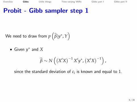
Probit - Gibb sampler step 1
We need to draw from p(
β|y∗, Y)
• Given y∗ and X
β ∼ N((
X′X)−1 X′y∗,
(X′X
)−1)
,
since the standard deviation of εi is known and equal to 1.
8 / 38
Overview Gibbs Little things Time-varying VARs Gibbs part I Gibbs part II
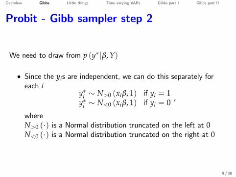
Probit - Gibb sampler step 2
We need to draw from p (y∗|β, Y)
• Since the yis are independent, we can do this separately foreach i
y∗i ∼ N>0 (xiβ, 1) if yi = 1y∗i ∼ N<0 (xiβ, 1) if yi = 0 ,
whereN>0 (·) is a Normal distribution truncated on the left at 0N<0 (·) is a Normal distribution truncated on the right at 0
9 / 38

Overview Gibbs Little things Time-varying VARs Gibbs part I Gibbs part II
Wishart distribution
• generalization of Chi-square distribution to more variables
• X : n× p matrix; each row drawn from Np (0, Σ), where Σ isthe p× p variance-covariance matrix
• W = X′X ∼ Wp (Σ, n), i.e., the p-dimensional Wishart withscale matrix Σ and degrees of freedom n
• You get the Chi-square if p = 1 and Σ = 1
10 / 38
Overview Gibbs Little things Time-varying VARs Gibbs part I Gibbs part II
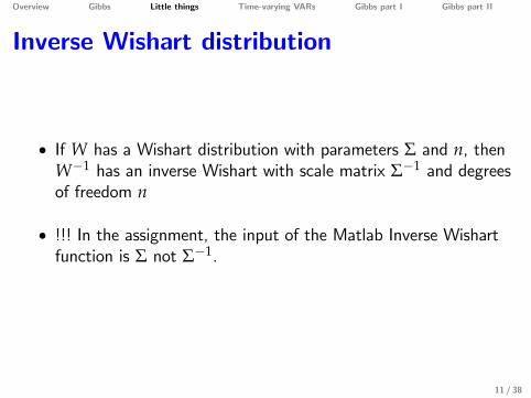
Inverse Wishart distribution
• If W has a Wishart distribution with parameters Σ and n, thenW−1 has an inverse Wishart with scale matrix Σ−1 and degreesof freedom n
• !!! In the assignment, the input of the Matlab Inverse Wishartfunction is Σ not Σ−1.
11 / 38

Overview Gibbs Little things Time-varying VARs Gibbs part I Gibbs part II
Inverse Wishart in Bayesian statistics• Data: xt is a p× 1 vector with i.i.d. random observations withdistribution N (0, V)
• prior of V :p (V) = IW
(V−1, n
)
• posterior of V :
p(
V|XT)= IW
(W−1, n+ T
)W = V+ VT
VT =T
∑t=1
x′txt
Note that VT is like a sum of squares12 / 38

Overview Gibbs Little things Time-varying VARs Gibbs part I Gibbs part II
Multivariate normal in Matlab
• xt is a p× 1 vector and we want xt ∼ N(0, Σ)
• C=chol(Σ)Thus C is an upper-triangular matrix and C′C = Σ
• et is a p× 1 vector with draws from N(0, Ip)
E[C′ete′tC
]= Σ
• Thus, C′et is a p× 1 vector with draws from N(0, Σ)
13 / 38

Overview Gibbs Little things Time-varying VARs Gibbs part I Gibbs part II
Time-varying VARs - intro
• Idea: capture changes in model specification in a flexible way
• The analysis here is based on Cogley and Sargent (2002), CS
14 / 38
Overview Gibbs Little things Time-varying VARs Gibbs part I Gibbs part II
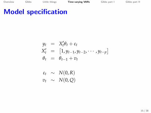
Model specification
yt = X′tθt + εt
X′t =[1, yt−1, yt−2, · · · , yt−p
]θt = θt−1 + vt
εt ∼ N(0, R)vt ∼ N(0, Q)
15 / 38

Overview Gibbs Little things Time-varying VARs Gibbs part I Gibbs part II
Model specification
Et
[εtvt
] [εt vt
]= V =
(R C′
C Q
)• θt : "parameters"• R, C, and Q are the "hyperparameters"
16 / 38

Overview Gibbs Little things Time-varying VARs Gibbs part I Gibbs part II
Model specification - details
Simplifying assumptions:
• CS impose that θt is such that yt would be stationary ifθt+τ = θt for all τ ≥ 0. This stationarity requirement is left outfor transparency.
• C = 0.
17 / 38

Overview Gibbs Little things Time-varying VARs Gibbs part I Gibbs part II
Notation
YT =[y′1, · · · , y′T
]θT =
[θ′0, θ′1, · · · , θ′T
]
18 / 38

Overview Gibbs Little things Time-varying VARs Gibbs part I Gibbs part II
Priors
• Prior for initial condition:
θ0 ∼ N(θ, P)
• Prior for hyperparameters:
p(V) = IW(
V−1, T0
)
• θ, P, V, T0 are taken as given
19 / 38
Overview Gibbs Little things Time-varying VARs Gibbs part I Gibbs part II
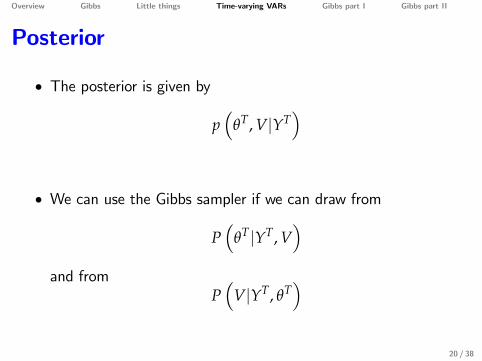
Posterior
• The posterior is given by
p(
θT, V|YT)
• We can use the Gibbs sampler if we can draw from
P(
θT|YT, V)
and fromP(
V|YT, θT)
20 / 38

Overview Gibbs Little things Time-varying VARs Gibbs part I Gibbs part II
Stationarity
• CS exclude draws of θt for which the dgp of yt is nonstationary:
• p (θt|·) is density without imposing stationarity and• f (θt|·) is density with imposing stationarity
• This restriction is ignored in these slides
21 / 38
Overview Gibbs Little things Time-varying VARs Gibbs part I Gibbs part II
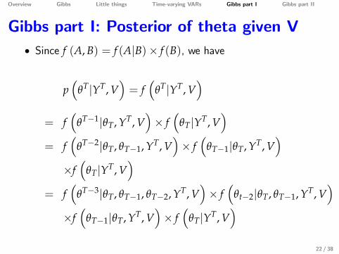
Gibbs part I: Posterior of theta given V• Since f (A, B) = f (A|B)× f (B), we have
p(
θT|YT, V)= f
(θT|YT, V
)= f
(θT−1|θT, YT, V
)× f
(θT|YT, V
)= f
(θT−2|θT, θT−1, YT, V
)× f
(θT−1|θT, YT, V
)×f(
θT|YT, V)
= f(
θT−3|θT, θT−1, θT−2, YT, V)× f
(θt−2|θT, θT−1, YT, V
)×f(
θT−1|θT, YT, V)× f
(θT|YT, V
)22 / 38
Overview Gibbs Little things Time-varying VARs Gibbs part I Gibbs part II
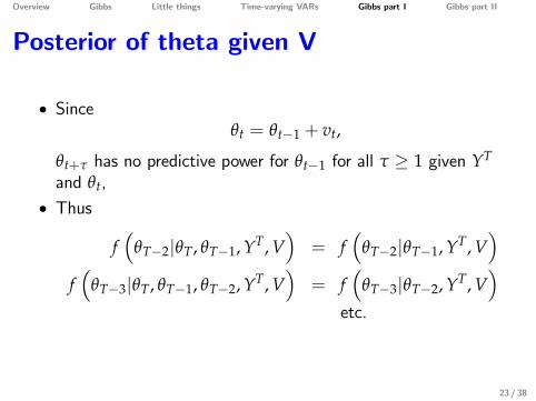
Posterior of theta given V
• Sinceθt = θt−1 + vt,
θt+τ has no predictive power for θt−1 for all τ ≥ 1 given YT
and θt,• Thus
f(
θT−2|θT, θT−1, YT, V)= f
(θT−2|θT−1, YT, V
)f(
θT−3|θT, θT−1, θT−2, YT, V)= f
(θT−3|θT−2, YT, V
)etc.
23 / 38
Overview Gibbs Little things Time-varying VARs Gibbs part I Gibbs part II
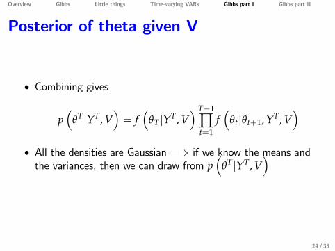
Posterior of theta given V
• Combining gives
p(
θT|YT, V)= f
(θT|YT, V
) T−1
∏t=1
f(
θt|θt+1, YT, V)
• All the densities are Gaussian =⇒ if we know the means andthe variances, then we can draw from p
(θT|YT, V
)
24 / 38
Overview Gibbs Little things Time-varying VARs Gibbs part I Gibbs part II
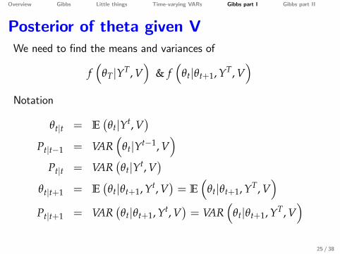
Posterior of theta given VWe need to find the means and variances of
f(
θT|YT, V)
& f(
θt|θt+1, YT, V)
Notation
θt|t = E(θt|Yt, V
)Pt|t−1 = VAR
(θt|Yt−1, V
)Pt|t = VAR
(θt|Yt, V
)θt|t+1 = E
(θt|θt+1, Yt, V
)= E
(θt|θt+1, YT, V
)Pt|t+1 = VAR
(θt|θt+1, Yt, V
)= VAR
(θt|θt+1, YT, V
)25 / 38
Overview Gibbs Little things Time-varying VARs Gibbs part I Gibbs part II
Posterior of theta given V
• First, use Kalman filter to go forward• start with θ0 and P0|0
• Next, go backwards to get draws for θt given θt+1
26 / 38

Overview Gibbs Little things Time-varying VARs Gibbs part I Gibbs part II
Posterior of theta given V• Kalman filter part:
yt = X′tθt + εt
X′t =[1, yt−1, yt−2, · · · , yt−p
]θt = θt−1 + vt
εt ∼ N(0, R)vt ∼ N(0, Q)
• Here:• the p+ 1 elements of Xt are the known (time-varying)coeffi cients of the state-space represenation
• the elements of θt are the unobserved underlying state variables27 / 38

Overview Gibbs Little things Time-varying VARs Gibbs part I Gibbs part II
Posterior of theta given V• Kalman filter in the first period:
P1|0 = P0|0 +Q
K1 = P1|0X1
(X′1P1|0X1 + R
)−1
θ1|1 = θ0|0 + K1
(y1 −X′1θ0|0
)• and then iterate
Pt|t−1 = Pt−1|t−1 +Q
Kt = Pt|t−1Xt
(X′tPt|t−1Xt + R
)−1
θt|t = θt−1|t−1 + Kt
(yt −X′tθt−1|t−1
)Pt|t = Pt|t−1 − KtX′tPt|t−1
28 / 38

Overview Gibbs Little things Time-varying VARs Gibbs part I Gibbs part II
Posterior of theta given V
• In the Kalman filter part of the assignment:
TH(:,1) = θ0
TH(:,t+1) = θt|tPe(:,:,t) = Pt−1|t−1
Po(:,:,t) = Pt|t−1
• and we go up to
TH(:,T+1) = θT|TPe(:,:,T+1) = PT|TPo(:,:,T) = PT|T−1
29 / 38

Overview Gibbs Little things Time-varying VARs Gibbs part I Gibbs part II
Posterior of theta given V
• Distribution terminal state:
f(
θT|YT, V)= N
(θT|T, PT|T
)
• From this we get a draw θT
30 / 38

Overview Gibbs Little things Time-varying VARs Gibbs part I Gibbs part II
Posterior of theta given V• Draws for θT−1, θT−2, · · · , θ1 are obtained recursively from
f(
θt|θt+1, YT, V)= N
(θt|t+1, Pt|t+1
)θt|t+1 = θt|t + Pt|tP
−1t+1|t
(θt+1 − θt|t
)Pt|t+1 = Pt|t − Pt|tP
−1t+1|tPt|t
• The terms needed to calculate θt|t+1 and Pt|t+1 are generatedby the Kalman filter (that is, from going forward) and thestandard projection formulas (and note that the covariance ofθt+1 and θt is the variance of θt)
31 / 38

Overview Gibbs Little things Time-varying VARs Gibbs part I Gibbs part II
Details for previous slide
E [y|x] = µy + ΣyxΣ−1xx (x− µx)
=⇒E [θt|θt+1; ·] = E [θt|·] + Σθtθt+1Σ−1
θt+1θt+1(θt+1 −E [θt+1|·])
= E [θt|·] + ΣθtθtΣ−1θt+1θt+1
(θt+1 −E [θt+1|·])=⇒
θt|t+1 = θt|t + Pt|tP−1t+1|t (θt+1 −E [θt + vt|·])
= θt|t + Pt|tP−1t+1|t (θt+1 −E [θt|·])
= θt|t + Pt|tP−1t+1|t
(θt+1 − θt|t
)Suppressing the dependence on Yt and V to simplify notation
32 / 38

Overview Gibbs Little things Time-varying VARs Gibbs part I Gibbs part II
Posterior of theta given VIn the backward part of the assignment:
Draw from TH(t-1|t)In the for loop below t goes from high to low.At a particular t:
1 TH(:,t+1) it is a random draw from a normal thathas already been determined (either in this loopor for T above)
2 TH(:,t) on the RHS of the mean equation is equalto theta_(t-1)|(t-1)
3 TH(:,t) what we end up with is a random draw fortheta(t-1) conditional on knowning theta in thenext period
33 / 38

Overview Gibbs Little things Time-varying VARs Gibbs part I Gibbs part II
Why go forward & backward?
• The Kalman filter gives us E(θt|Yt, V
)and VAR(θt|Yt, V)
• With this information, we can also obtain draws for θt
• However, we need draws from f(
θT|YT, V)not from
f(
θT|Yt, V). The analysis above showed how to get draws
from f(
θT|YT, V)recursively by going backward.
34 / 38

Overview Gibbs Little things Time-varying VARs Gibbs part I Gibbs part II
Relation to Kalman Smoother
• The Kalman smoother also goes backwards and resembles theprocedure here.
• However, there is a difference.• The Kalman smoother computes the mean and variance for
f(θt|YT, V
)• We need the mean and variance for f
(θt|θt+1, YT, V
)• Since
f(
θt|θt+1, YT, V)= f
(θt|θt+1, Yt, V
),
we can calculate these from Kalman filter without using theKalman smoother
35 / 38

Overview Gibbs Little things Time-varying VARs Gibbs part I Gibbs part II
Gibbs part II: Posterior of V given theta
• Next step is to draw from the posterior given YT and θT, thatis get a draw from p
(V|YT, θT
)• The posterior combines the prior and information from the data=⇒ in each Gibbs iteration the prior is the same but the dataset (i.e., θT) is different
36 / 38

Overview Gibbs Little things Time-varying VARs Gibbs part I Gibbs part II
Gibbs part II: Posterior of V given theta• Given YT and θT, we can calcluate εt and νt.
• Both have mean zero and a Normal distribution
• Thus
p(
V|YT, θT)= IW(V−1
1 , T1)
T1 = T0 + TV1 = V+VT
VT =T
∑t=1
(εtvt
) (ε′t v′t
)!!! Note that V, VT, &V1 are like a sum of squares, whereas V(and R&Q) are like a sum of squares divided by number ofobservations (same notation as in CS)
37 / 38

Overview Gibbs Little things Time-varying VARs Gibbs part I Gibbs part II
References
• Casella, G., and E.I. George, 1992, Explaining the Gibbs Sampler, The American
Statistician, 46 167-74.
• Cogley, T. and T.J. Sargent, 2001, Evolving Post-World War II U.S. Inflation Dynamics,
NBER Macroeconomics Annual 2001, volume 16, 331-338.
• De Wind, J, 2014, Accounting for time-varying and nonlinear relationships in
macroeconomic models, dissertation, University of Amsterdam. Available at
http://dare.uva.nl/document/523663.
• Lancaster, T., 2004, An introduction to modern Bayesian econometrics, Blackwell
Publishing.
• very nice textbook covering lots of stuff in an understandable way
38 / 38