Time-Varying Quantiles

Giuliano De Rossi and Andrew HarveyFaculty of Economics, Cambridge University

e-mail: ach34@cam.ac.uk

January 31, 2007

1 Introduction

In modelling the evolution of a time series, we may wish to take account ofchanges in many aspects of the distribution over time rather than in justthe mean or, as is often the case in �nance, the variance. In a cross-section,the sample quantiles provide valuable and easily interpretable information;indeed if enough of them are calculated they e¤ectively provide a compre-hensive description of the whole distribution. It is not di¢ cult to capture theevolution of such quantiles over time. For example, Harvey and Bernstein(2003) use standard unobserved component (UC) models to extract under-lying trends from the time series of quantiles computed for the U.S. wagedistribution.Estimating time-varying quantiles for a single series is far more di¢ cult.

The problem is a fundamental one from the statistical point of view. Fur-thermore it is of considerable practical importance, particularly in areas like�nance where questions of, for example, value at risk (VaR) appeals directlyto a knowledge of certain quantiles of portfolio returns; see the RiskMetricsapproach of J.P. Morgan (1996) and the discussion in Christo¤ersen, Hahnand Inoue (2001). Engle and Manganelli (2004) highlight this particular is-sue, as do Chernozhukov and Umantsev (2001). They propose the use ofvarious nonlinear conditional autoregressive value at risk (CAViaR) modelsto make one-step ahead predictions of VaR in time series of stock returns.These models are based on quantile regression (QR); see the recent mono-graph by Koenker (2005). As with linear quantile autoregressions (QARs),

1

the properties and applications of which have recently been investigated byKoenker and Xiao (2004, 2006), the conditioning on past observations en-ables estimation to be carried out by standard QR estimation procedures,usually based on linear programming, and the construction of forecasts isimmediate. Engle and Manganelli have to resort to trying to capture the be-havior of tail quantiles in returns by nonlinear functions of past observationsbecause linear functions lack the necessary �exibility. But in doing so theyencounter a fundamental problem, namely what functional form should bechosen? A good deal of their article is concerned with devising methods fordealing this issue.Treating the problem as one of signal extraction provides an altogether

di¤erent line of attack. Estimating quantiles in this way provides a descrip-tion of the series, while the estimates at the end form the basis for predictions.This approach seems entirely natural and once it is adopted a much clearer in-dication is given as to the way in which past observations should be weightedfor prediction in a nonlinear quantile autoregression. The motivation forwhat we are doing is provided by the simplest case, namely stock marketreturns. The base model is that returns are independently and identicallydistributed (IID). By allowing the quantiles to evolve over time, it becomespossible to capture a changing distribution. Movements may be stationaryor non-stationary, but they will usually be slowly changing. Figure 1 shows2000 daily returns for General Motors1 together with smoothed estimates forquantiles obtained from a model that assumes that they are generated byrandom walks. The implications for forecasting are obvious.The distinction between models motivated by description and those set up

to deal directly with prediction is a fundamental one in time series. Structuraltime series models (STMs) are formulated in terms of unobserved compo-nents, such as trends and cycles, that have a direct interpretation; see Harvey(1989). Signal extraction, or smoothing, provides estimates of these compo-nents over the whole sample, while the (�ltered) estimates at the end providethe basis for nowcasting and forecasting. Autoregressive and autoregressive-

1The stock returns data used as illustrations are taken from Engle and Manganelli(2004). Their sample runs from April 7th, 1986, to April 7th, 1999. The large (absolute)values near the beginning of �gure 1 are associated with the great crash of 1987.The histogram of the series from observation 501 to 2000 (avoiding the 1987 crash)

shows heavy tails but no clear evidence of skewness. The excess kurtosis is 1.547 and theassociated test statistic, distributed as �21 under normality, is 149.5. On the other hand,skewness is 0.039 with an associated test statistic of only 0.37.

2

0 150 300 450 600 750 900 1050 1200 1350 1500 1650 1800 1950

­20

­15

­10

­5

0

5

10

GMQ(05)Q(95)

Q(25)Q(75)

Figure 1: Quantiles �tted to GM returns

integrated-moving average (ARIMA) models, on the other hand, are con-structed primarily with a view to forecasting. In a linear Gaussian world,the reduced form of an STM is an ARIMAmodel and questions regarding themerits of STMs for forecasting revolve round the gains, or losses, from theimplied restrictions on the reduced form and the guidance, or lack of it, givento the selection of a suitable model; see the discussion in Harvey (2006) andDurbin and Koopman (2001). Once nonlinearity and non-Gaussianity enterthe picture, the two approaches can be very di¤erent. For example, chang-ing variance can be captured by a model from the generalized autoregressiveconditional heteroscedasticity (GARCH) class, where conditional varianceis a function of past observations, or by a stochastic volatility (SV) modelin which the variance is a dynamic unobserved component; see the recentcollection of readings by Shephard (2005).Section 2 of the paper reviews the basic ideas of quantiles and QR and

notes that the criterion of choosing the estimated quantile so as to minimizethe sum of absolute values around it can be obtained from a model in whichthe observations are generated by an asymmetric double exponential distri-bution. In section 3 this distribution is combined with a time series model,such as a stationary �rst-order autoregressive process or a random walk, to

3

produce the criterion function used as the basis for extracting time-varyingquantiles. Di¤erentiating this criterion function leads to a set of equationswhich, when solved, generalize the de�ning characteristic of a sample quantileto the dynamic setting. We outline an algorithm for computing the quan-tiles. The algorithm iterates the Kalman �lter and associated (�xed-interval)smoother until convergence, taking special care in the way it deals with cuspsolutions, that is when a quantile passes through an observation. The modelsfor the quantiles usually depend on only one or two parameters and theseparameters be estimated by cross-validation.Section 4 details the various aspects of a distribution that can be cap-

tured by time�varying quantiles. We �rst note that the inter-quartile rangeprovides an alternative to GARCH and SV models for estimating and pre-dicting dispersion and that the assumptions needed to compute it are muchless restrictive. We then go on to observe that di¤erent quantile-based rangescan provide constrasts between movements near the centre of the distribu-tion and those near the tails. Other contrasts can be designed to captureasymmetries, while the 1% and 5% quantiles provide estimates of VaR. En-gle and Manganelli (2004, p369) observe, in connection with CAViaR models,that one of their attractions is that they are useful �..for situations with con-stant volatilities but changing error distributions..� The same is true of ourtime-varying quantiles for the lower tails.Section 5 sets out a stationarity test for the null hypothesis that a quantile

is time-invariant against the alternative that it is slowly changing. This testis based on binomial quantile indicators - sometimes called �quantile hits�-and is a generalization of a test proposed by DeJong, Amsler and Schmidt(2005) for the constancy of the median. Tests2 for the constancy of contrastsbetween quantiles are illustrated with data on returns. A full invetigationinto the properties of the tests can be found in Busetti and Harvey (2007).QAR and CAViaR models are discussed in section 6. We suggest that

conditional autoregressive speci�cations, especially linear ones, are in�uencedtoo much by Gaussian notions even though on the surface the emphasis onquantiles appears to escape from Gaussianity. One consequence is that thesemodels may not be robust to additive outliers. The functional forms proposedby Engle and Manganelli (2004) are assessed with respect to robustness andcompared with speci�cations implied by the signal extraction approach. A

2Linton and Whang (2006) have studied the properties of the quantilogram, the cor-relogram of the quantile hits, and an associated portmanteau test.

4

way of combining the two approaches then emerges.So far as we know, the only work which is related to our approach to

extracting time-varying quantiles is by Bosch et al (1995). Their paper con-cerns cubic spline quantile regression and since they do not apply it to timeseries the connections may not be apparent. Bosch et al (1995) propose aquadratic programming algorithm, but this appears to be very computation-ally intensive. We show in section 7 that the stochastic trend models that weused earlier lead to estimated quantiles that are, in fact, splines. Our statespace smoothing algorithm can be applied to cubic spline quantile regressionby modifying it to deal with irregular observations. This method of dealingwith splines is well known in the time series literature and its extension toquantile regression may prove useful.

2 Quantiles and quantile regression

Let Q(�) - or, when there is no risk of confusion, Q - denote the � � thquantile. The probability that an observation is less than Q(�) is � ; where0 < � < 1: Given a set of T observations, yt; t = 1; ::; T; (which may be froma cross-section or a time series), the sample quantile, eQ(�); can be obtainedby sorting the observations in ascending order. However, it is also given asthe solution to minimizing

S(�) =Xt

�� (yt �Q) =Xyt<Q

(� � 1)(yt �Q) +Xyt�Q

�(yt �Q)

=Xt

(� � I(yt �Q < 0)) (yt �Q)

with respect to Q; where �� (:) is the check function and I(:) is the indicatorfunction. Di¤erentiating (minus) S(�) at all points where this is possiblegives X

IQ(yt �Q(�));

where

IQ(yt �Qt(�)) =�� � 1; if yt < Qt(�)� ; if yt > Qt(�)

(1)

de�nes the quantile indicator function for the more general case where thequantile may be time-varying. Since �� (:) is not di¤erentiable at zero, the

5

quantile indicator function is not continuous at 0 and IQ(0) is not deter-mined.3

The sample quantile, eQ(�); is such that, if T� is an integer, there are T�observations below the quantile and T (1��) above. In this case any value ofeQ between the T� � th smallest observation and the one immediately abovewill make

PIQ(yt � eQ) = 0: If T� is not an integer, eQ will coincide with

one observation. This observation is the one for whichPIQ(yt� eQ) changes

sign. These statements need to be modi�ed slightly if several observationstake the same value and coincide with eQ: Taking this point on board, ageneral de�nition of a sample ��quantile is a point such that the number ofobservations smaller, that is yt < eQ; is no more than [T� ] while the numbergreater is no more than [T (1� �)]:When yt = eQ we will assign IQ(yt � eQ) a value that makes the sum of

the IQ(yt � eQ)0s equal to zero. This has the additional attraction that itenables us to think of the condition

PIQ(yt � eQ) = 0 as characterizing a

sample quantile in much the same way asP(yt � e�) = 0 de�nes a method

of moments estimator, e�; for a mean.In quantile regression, the quantile, Qt(�); corresponding to the t � th

observation is a linear function of explanatory variables, xt; that is Qt = x0t�.The quantile regression estimates are obtained by minimizing

Pt �� (yt�x0t�)

with respect to the parameter vector �: Estimates may be computed by linearprogramming as described in Koenker (2005). In quantile autoregression Qtis a linear combination of past observations.Finally suppose that the observations are assumed to come from an asym-

metric double exponential distribution

p(ytjQt) = �(1� �)!�1 exp(�!�1�� (yt �Qt)); (2)

where ! is a scale parameter. Maximising the log-likelihood function is equiv-alent to minimising the criterion function

S(�) =Xt

�� (yt �Qt): (3)

Thus the model, (2), de�nes Qt as a (population) quantile by the conditionthat the probability of a value below is � while the form of the distributionleads to the maximum likelihood (ML) estimator satisfying the conditions

3Hence we have not written IQt = (� � I(yt �Q < 0)):

6

for a sample quantile, when Q is constant, or a quantile regression estimate.Since quantiles are �tted separately, there is no notion of an overall modelfor the whole distribution and assuming the distribution (2) for one quantileis not compatible with assuming it for another. Setting up this particularparametric model is simply a convenient device that leads to the appropriatecriterion function for what is essentially a nonparametric estimate.

3 Signal extraction

A model-based framework for estimating time-varying quantiles, Qt(�); canbe set up by assuming that they are generated by a Gaussian stochasticprocess and are connected to the observations through a measurement equa-tion

yt = Qt(�) + "t(�); t = 1; :::; T; (4)

where Pr(yt � Qt < 0) = Pr("t < 0) = � with 0 < � < 1: The problemis then one of signal extraction with the model for Qt(�) being treated asa transition equation. By assuming that the disturbance term, "t; has anasymmetric double exponential distribution, as in (2), we end up choosingthe estimated quantiles so as to minimise

Pt �� (yt �Qt) subject to a set of

constraints imposed by the time series model for the quantile.We will focus attention on three time series models, all of which are able

to produce quantiles that change relatively slowly over time with varyingdegrees of smoothness. The theory can be applied to any linear time seriesmodel, but it will often be the case that prior notions on the behaviour ofthe quantile play an important role in speci�cation.

3.1 Models for evolving quantiles

The simplest model for a stationary time-varying quantile is a �rst-orderautoregressive process

Qt(�) = (1� �)Qy� + ��Qt�1(�) + �t(�); j�� j < 1; t = 1; :::; T; (5)

where �t(�) is normally and independently distributed with mean zero andvariance �2�(�); that is �t(�) � NID(0; �2�(�)); �� is the autoregressive para-

7

meter and Qy� is the unconditional mean of Qt(�). In what follows the �appendage will be dropped where there is no ambiguity.The random walk quantile is obtained by setting � = 1 so that

Qt = Qt�1 + �t; t = 2; :::; T:

The initial value, Q1, is assumed to be drawn from a N(0; �) distribution.Letting � ! 1 gives a di¤use prior; see Durbin and Koopman (2001). Anonstationary quantile can also be modelled by a local linear trend

Qt = Qt�1 + �t�1 + �t (6)

�t = �t�1 + �t

where �t is the slope and �t is NID(0; �2�). It is well known that in a

Gaussian model setting

V ar

��t�t

�= �2�

�1=3 1=21=2 1

�(7)

results in the smoothed estimates being a cubic spline. (In practice, theintegrated random walk (IRW), obtained by suppressing �t; gives very similarresults). The spline connection will be taken up further in section 8.

3.2 Theory

If we assume an asymmetric double exponential distribution for the distur-bance term in (4) and let the quantile be a �rst-order autoregression, as in(5), the logarithm of the joint density for the observations and the quantilesis, ignoring terms independent of quantiles,

J = log p(y1; ::; yT ; Q1; ::; QT )

= �12

(1� �2)(Q1 �Qy)2�2�

� 12

TXt=2

�2t�2��

TXt=1

�� (yt �Qt)!

: (8)

Given the observations, the estimated time-varying quantiles, eQ1; ::; eQT ; arethe values of the Q0ts that maximise J: In other words they are the conditionalmodes.When "t is NID(0; �2) we may replace Qt by the mean, �t; and write

yt = �t + "t; t = 1; :::; T (9)

8

and J is rede�ned with �� (yt�Qt)=! in (8) replaced by (yt��t)2=2�2: Di¤er-entiating J with respect to �t; t = 1; :::; T; setting to zero and solving givesthe modes, e�t; t = 1; :::; T; of the conditional distributions of the �0ts: Fora multivariate Gaussian distribution these are the conditional expectations,which by de�nition are the smoothed (minimum mean square error) estima-tors. They may be e¢ ciently computed by the Kalman �lter and associatedsmoother; see de Jong (1989) and Durbin and Koopman (2001).Returning to the quantiles and di¤erentiating with respect to Qt gives

@J

@Qt=�Qt�1 � (1 + �2)Qt + �Qt+1 + (1� �)2Qy

�2�+1

!IQ (yt �Qt) ; (10)

for t = 2; : : : ; T � 1, and, at the endpoints,

@J

@Q1= �(1� �

2)(Q1 �Qy)�2�

+[� (Q2 � �Q1)� �(1� �)Qy]

�2�+1

!IQ (y1 �Q1)

and@J

@QT=� (QT � �QT�1) + (1� �)Qy

�2�+1

!IQ (yT �QT )

where IQ (yt �Qt) is de�ned as in (1). For t = 2; ::; T �1; setting @J=@Qt tozero gives an equation that is satis�ed by the estimated quantiles, eQt; eQt�1and eQt+1; and similarly for t = 1 and T . If a solution is on a cusp, thatis eQt = yt; then IQ (yt �Qt) is not de�ned as the check function is notdi¤erentiable at zero. Note that, when it does exist, the second derivative isnegative.For the random walk we can write the �rst term as �Q12=2� and let

� ! 1; noting that � = �2�=(1 � �2): The derivatives of J are a simpli�edversion of those in (10) with the �rst term in @J=@Q1 dropping out. It iseasy to see that the terms associated with the random walk, that is ignoringthe IQ0ts; sum to zero. On the other hand, when Qt is stationary, summingthe terms in the derivatives not involving the IQ0ts yields

�(1� �)Q1 � (1� �)2X

Qt � (1� �)QT + (T � 2)(1� �)2Qy + 2(1� �)Qy

divided by �2�: However, setting

eQy = (1� �)( eQ1 + eQT ) + (1� �)2PT�1t=2

eQt(T � 2)(1� �)2 + 2(1� �) (11)

9

ensures that the sum is zero at the mode. The mean in the Gaussian modelneeds to be estimated in a similar way if the residuals, yt � e�t; t = 1; :::; T;are to sum to zero.Establishing that the derivatives of that part of the criterion function

associated with the time series model for the quantile sum to zero enables usto establish a fundamental property of time-varying quantiles, namely thatthe number of observations that are less than the corresponding quantile, thatis yt < eQt; is no more than [T� ] while the number greater is no more than[T (1� �)]: A general proof can be found in De Rossi and Harvey (2007).A similar property can be obtained for regression quantiles. However,

as Koenker (2005, p35-7) observes, the number of cusps rarely exceeds thenumber of explanatory variables.Finally note that when the signal-noise ratio is zero, that is �2� = 0; there

is usually only one cusp, while for a value of in�nity, obtained when ! = 0;there are T cusps as all quantiles pass through all observations.

3.3 The form of the solution

In a Gaussian model, (9), a little algebra leads to the classicWiener-Kolmogorov(WK) formula for a doubly in�nite sample. For the AR(1) model

e�t = �+ g

gy(yt � �)

where � = E(�t); g = �2�=((1 � �L)(1 � �L�1)) is the autocovariance gen-erating function (ACGF), L is the lag operator, and gy = g + �2": The WKformula has the attraction that for simple models g=gy can be expanded togive an explicit expression for the weights. Here

e�t = �+ q��

�(1� �2)

1Xj=�1

�jjj(yt+j � �) (12)

where q� = �2�=�2" and � = (q� + 1+ �

2)=2��h�q� + 1 + �

2�2 � 4�2i1=2 =2�.

This expression is still valid for the random walk except that � disappearsbecause the weights sum to one.In order to proceed in a similar way with quantiles, we need to take

account of cusp solutions by de�ning the corresponding IQ0ts as the values

10

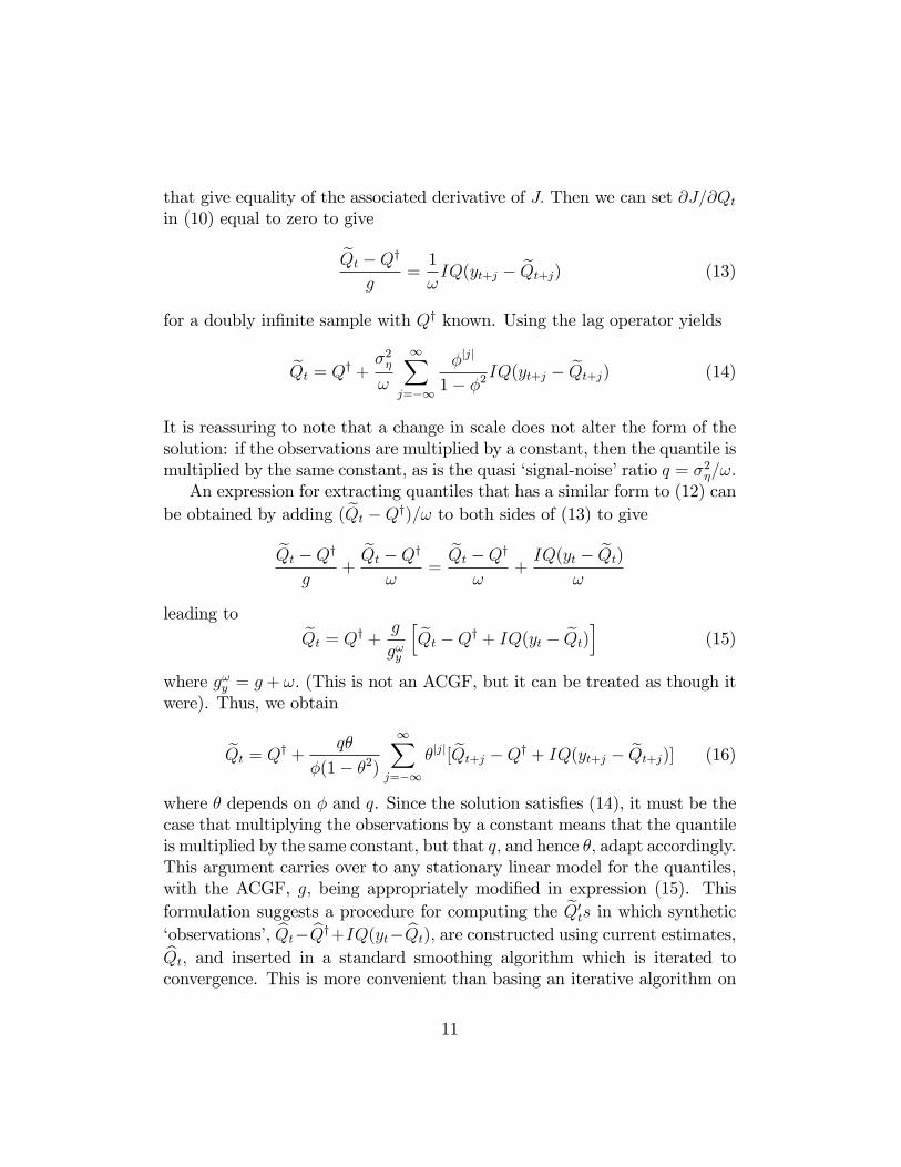
that give equality of the associated derivative of J: Then we can set @J=@Qtin (10) equal to zero to give

eQt �Qyg

=1

!IQ(yt+j � eQt+j) (13)

for a doubly in�nite sample with Qy known. Using the lag operator yields

eQt = Qy + �2�!

1Xj=�1

�jjj

1� �2IQ(yt+j � eQt+j) (14)

It is reassuring to note that a change in scale does not alter the form of thesolution: if the observations are multiplied by a constant, then the quantile ismultiplied by the same constant, as is the quasi �signal-noise�ratio q = �2�=!.An expression for extracting quantiles that has a similar form to (12) can

be obtained by adding ( eQt �Qy)=! to both sides of (13) to giveeQt �Qyg

+eQt �Qy!

=eQt �Qy!

+IQ(yt � eQt)

!

leading to eQt = Qy + g

g!y

h eQt �Qy + IQ(yt � eQt)i (15)

where g!y = g + !: (This is not an ACGF, but it can be treated as though itwere). Thus, we obtain

eQt = Qy + q�

�(1� �2)

1Xj=�1

�jjj[ eQt+j �Qy + IQ(yt+j � eQt+j)] (16)

where � depends on � and q. Since the solution satis�es (14), it must be thecase that multiplying the observations by a constant means that the quantileis multiplied by the same constant, but that q; and hence �; adapt accordingly.This argument carries over to any stationary linear model for the quantiles,with the ACGF, g; being appropriately modi�ed in expression (15). Thisformulation suggests a procedure for computing the eQ0ts in which synthetic�observations�, bQt� bQy+IQ(yt� bQt); are constructed using current estimates,bQt; and inserted in a standard smoothing algorithm which is iterated toconvergence. This is more convenient than basing an iterative algorithm on

11

(14). In the middle of a large sample, smoothing corresponds to the repeatedapplication of (16).For the random walk, (10) becomes

� eQt�1 + 2 eQt � eQt+1 = �2 eQt+1 = �2�!IQ(yt � eQt)

and expression (14) can no longer be obtained. Since the weights in (16) sumto one, Qy drops out giving

eQt = 1� �1 + �

1Xj=�1

�jjj[ eQt+j + IQ(yt+j � eQt+j)] (17)

Thus standard smoothing algorithms can be applied to the synthetic obser-vations, bQt + IQ(yt � bQt):When the quantiles change over time they may be estimated non-parametrically.

The simplest option is to compute them from a moving window; see, for ex-ample, Kuester et al (2006). More generally a quantile may be estimated atany point in time by minimising a local check function, that is

minhX

j=�h

K(j

h)�� (yt+j �Qt)

where K(:) is a weighting kernel and h is a bandwidth; see Yu and Jones(1998). Di¤erentiating with respect to Qt and setting to zero de�nes anestimator, bQt; in the same way as was done in section 2. That is bQt mustsatisfy

hXj=�h

K(j

h)IQ(yt+j � bQt) = 0

with IQ(yt+j� bQt) de�ned appropriately if yt+j = bQt: Adding and subtractingbQt to each of the IQ(yt+j � bQt) terms in the sum, leads tobQt = 1Ph

j=�hK(j=h)

hXj=�h

K(j

h)[ bQt + IQ(yt+j � bQt)]:

It is interesting to compare this with the weighting scheme implied by therandom walk model where K(j=h) is replaced by �jjj so giving an (in�nite)

12

exponential decay. An integrated random walk implies a kernel with a slowerdecline for the weights near the centre; see Harvey and Koopman (2000). Thetime series model determines the shape of the kernel while the signal-noiseratio plays the same role as the bandwidth. Note also that in the model-basedformula, bQt+j is used instead of bQt when j is not zero.Of course, the model-based approach has the advantage that it auto-

matically determines a weighting pattern at the end of the sample that isconsistent with the one in the middle.

3.4 Algorithms for computing time-varying quantiles

An algorithm for computing time-varying quantiles needs to �nd values ofeQt; t = 1; ::; t; that set each of the derivatives of J in (10) equal to zero whenthe corresponding eQt is not set equal to yt: The algorithm described in DeRossi and Harvey (2006) combines an iterated state space smoother with asimpler algorithm that takes account of cusp solutions. It is suggested thatparameters be estimated by cross-validation.

4 Dispersion, Asymmetry and Value at Risk

The time-varying quantiles provide a comprehensive description of the dis-tribution of the observations and the way it changes over time. The choiceof quantiles will depend on what aspects of the distribution are to be high-lighted. The lower quantiles, in particular 1% and 5%, are particularly im-portant in characterizing value at risk over the period in question. A contrastbetween quantiles may be used to focus attention on changes in dispersionor asymmetry.

4.1 Dispersion

The contrasts between complementary quantiles, that is

D(�) = Qt(1� �)�Qt(�); � < 0:5; t = 1; ::; T

yield measures of dispersion. A means of capturing an evolving interquartilerange, D(0:25); provides an alternative to GARCH and stochastic volatil-ity models. As Bickel and Lehmann (1976) remark �Once outside the nor-mal model, scale provides a more natural measure of dispersion than vari-

13

0 50 100 150 200 250

0.00125

0.00150

0.00175

0.00200

0.00225

0.00250

0.00275

0.00300IQrange

Figure 2: Interquartile range for US in�ation

ance......and o¤ers substantial advantages from the robustness4 viewpoint�.Other contrasts may give additional information.Figure 2 shows the interquartile range for US in�ation.

4.1.1 Imposing symmetry

If the distribution is assumed to be symmetric around zero, better estimatesof Qt(�) and Qt(1 � �) can be obtained by assuming they are the same5.This can be done simply by estimating the (1� 2�)th quantile for jytj. Thusto compute eQt(0:75) = � eQt(0:25) we estimate the median for jytj : Doublingthis series gives the interquartile range.

4Koenker and Zhao (1996, p794) quote this observation and then go on to model scale(of a zero mean series) as a linear combination of past absolute values of the observations( rather than variance as a linear combination of past squares as in GARCH). They then�t the model by quantile regression. As we will argue later - in section 7 - this type ofapproach is not robust to additive outliers.

5A test of the null hypothesis that the observations are symmetric about zero could becarried out by noting that for IID observations eQ(1� �) + eQ(�) is asymptotically normalwith mean zero and variance (2� � �2)=f2(Q(�)):

14

0 150 300 450 600 750 900 1050 1200 1350 1500 1650 1800 1950

2.5

5.0

7.5

10.0

12.5

15.0

17.5

20.0

22.5

GMabQab(90)

Qab(50)

Figure 3: 25% and 5% quantiles estimated from absolute values of GM re-turns

Figure 3 shows absolute values and the resulting estimates of the sym-metric 5%/95% and 25%/75% quantiles for the raw series. The square rootsof q for the 5%/95% and 25%/75% quantiles were 0.11 and 0.06 respectively.(These are close to the values obtained for the individual corresponding quan-tiles, though it is not clear that they should necessarily be the same).Figure 4 shows estimates of the standard deviation of GM obtained by

�tting a random walk plus noise to the squared observations and then takingthe square root of the smoothed estimates6. These can be compared withthe estimates of the interquartile range and the 5%-95% range, obtained bydoubling the quantiles 50% and 90%, respectively, of the absolute value of theseries. Dividing the 5%-95% range by 3.25 is known to give a good estimateof the standard deviation for a wide range of distributions; see, for example,the recent study by Taylor (2005). Estimation was carried out using theobservations from 1 to 2000, but the graph shows 300 to 600 in order to

6This approach can be regarded as a combination of Riskmetrics and UC. EstimatingIGARCH parameters and using these to construct smoothed estimates (by calculating theimplied signal-noise ratio) can be expected to give a similar result, as will �tting an SVmodel.

15

300 350 400 450 500 550 600

2.5

5.0

7.5

10.0

12.5

15.0

17.5

20.0

22.5

GMabQab(90)

Qab(50)GMsqrt

Figure 4: 25% and 5% quantiles estimated from absolute values of GM re-turns, together with SD from smoothed squared observations

highlight the di¤erences emanating from the large outliers around 400. Ascan be seen the quantile ranges are less volatile than the variance estimates.

4.1.2 Tail dispersion

A comparison between the interquartile range and the interdecile range (0:1to 0:9); or the 0:05 to 0:95 range, could be particularly informative in pointingto di¤erent behaviour in the tails. These contrasts can be constructed withor without symmetry imposed.We generated 500 observations from a scale mixture of two Gaussian

distributions with time-varying weights and variances chosen so as to keepthe overall variance constant over time. Speci�cally, while the variance of the�rst component was set equal to one, the variance of the second componentwas allowed to increase, as a linear function of time, from 20 to 80. Theweights used to produce the mixture were adjusted so as to keep the overallvariance constant, at a value of ten. As a result, the shape of the distributionchanges during the sample period, with the tail dispersion decreasing, ascan be seen from the 5% quantile shown in �gure 5. The cross validation

16

0 50 100 150 200 250 300 350 400 450 500

­20

­15

­10

­5

0

5

10

15

20 Simulated dataTrue quantile

Estimated quantile

Figure 5: 5% quantile and estimate from simulated contaminated normaldistribution

procedure was then used to select the signal-noise ratio for RW model andextract the corresponding 5% quantile. The square root of the estimated ratiowas 0.1. As can be seen from �gure 5, it tracks the true quantile quite well(and an estimate based on absolute values would be even better) . When astochastic volatility model was estimated by quasi-maximum likelihood usingSTAMP, it produced a constant variance.As a second example we gradually changed the mixture in a contaminated

normal distribution to give the 5% quantile shown in �gure 6. The estimatedquantile is shown in �gure 7.Some notion of the way in which tail dispersion changes can be obtained

by plotting the ratio of the 0:05 to 0:95 range to the interquartile range(without imposing symmetry), that iseD(0:05)eD(0:25) = eQt(0:95)� eQt(0:05)eQt(0:75)� eQt(0:25) : (18)

For a normal distribution this ratio is 2.44, for t3 it is 3.08 and for a Cauchy6.31. Figure 8 shows the 5% and 25 % quantiles and the plot of (18) for theGM series.

17

0 200 400 600 800 1000 1200 1400 1600 1800 2000­10

­5

0

5

Returns True 5 % quantile

0 200 400 600 800 1000 1200 1400 1600 1800 2000

0 .1

0 .2

0 .3

0 .4

0 .5Weight on high variance component

Figure 6: Contaminated normal, variances one and nine with weight on thehigh variance component given by exp(�((t� 1000)=500)2)=2:

0 200 400 600 800 1000 1200 1400 1600 1800 2000­10 .0

­7 .5

­5 .0

­2 .5

0 .0

2 .5

5 .0

7 .5

Observations25%

5%

Figure 7: Estimates of 5% and 95% quantiles from data in previous �gure.

18

0 150 300 450 600 750 900 1050 1200 1350 1500 1650 1800 1950

2

4

6

D(05) D(25)

0 150 300 450 600 750 900 1050 1200 1350 1500 1650 1800 1950

2.5

3.0

3.5 R(05/25) Normal

Figure 8: Interquartile, 5%-95% range and (lower graph) their ratio

4.2 Asymmetry

For a symmetric distribution

S(�) = Qt(�) +Qt(1� �)� 2Qt(0:5); � < 0:5 (19)

is zero for all t = 1; ::; T . Hence a plot of this contrast shows how theasymmetry captured by the complementary quantiles, Qt(�) and Qt(1 � �)changes over time.If there is reason to suspect asymmetry, changes in tail dispersion can be

investigated by plotting

S(0:05=0:25) =eQt(0:05)� eQt(0:5)eQt(0:25)� eQt(0:5)

and similarly for eQt(0:75) and eQt(0:95):5 Tests of time invariance (IQ tests)

Before estimating a time-varying quantile it may be prudent to test the nullhypothesis that it is constant. Such a test may be based on the sample

19

quantile indicator or quantic, IQ(yt � eQ(�)): If the alternative hypothesis isthat Qt(�) follows a random walk, a modi�ed version of the basic stationaritytest is appropriate; see Nyblom and Mäkeläinen (1983) and Nyblom (1989).This test is usual applied to the residuals from a sample mean and because thesum of the residuals is zero, the asymptotic distribution of the test statistic isthe integral of squared Brownian bridges and this is known to be a Cramér-von Mises (CvM) distribution; the 1%, 5% and 10% critical values are 0.743,0.461 and 0.347 respectively. Nyblom and Harvey (2001) show that the testhas high power against an integrated random walk while Harvey and Streibel(1998) note that it is also has a locally best invariant (LBI) interpretationas a test of constancy against a highly persistent stationary AR(1) process.This makes it entirely appropriate for the kind of situation we have in mindfor time-varying quantiles.Assume that under the null hypothesis the observations are IID. The

population quantile indicators, IQ(yt � Q(�)); have a mean of zero and avariance of �(1 � �): The quantics sum to zero if, when an observation isequal to the sample quantile, the corresponding quantic is de�ned to ensurethat this is the case; see section 2. Hence the stationarity test statistic

�� =1

T 2�(1� �)

TXt=1

tXi=1

IQ(yi � eQ(�))!2 (20)

has the CvM distribution (asymptotically). De Jong, Amsler and Schmidt(2006) give a rigorous proof for the case of the median.7 Carrying over theirassumptions to the case of quantiles and IID observations we �nd that allthat is required is that Q(�) be the unique population ��quantile and thatyt �Q(�) has a continuous positive density in the neighbourhood of zero.Test statistics for GM are shown in the table below for a range of quan-

tiles. All (including the median) reject the null hypothesis of time invarianceat the 1% level of signi�cance. However, the test statistic for � = 0:01 isonly 0.289 which is not signi�cant at the 10% level. This is consistent withthe small estimate obtained for the signal-noise ratio. Similarly the statisticis 0.354 for � = 0:99 is only just signi�cant at the 10% level.

7De Jong, Amsler and Schmidt (2005) are primarily concerned with a more generalversion of the median test when there is serial correlation under the null hypothesis.Assuming strict stationarity (and a mixing condition) they modify the test of Kwiatkowskiet al (1992) - the KPSS test - so that it has the CvM distribution under the null. Similarmodi�cations could be made to quantile tests. More general tests, for both stationary andnonstationary series are currently under investigation.

20

� :05 :25 :50 :75 :95�� 1:823 1:026 2:526 1:544 2:962

De Jong et al (2005) also reject constancy of the median for certain weeklyexchange rates. The stationarity test with no correction for serial correlationdoes not reject in these cases. The same is true here as its value is only 0.146.A plot of the estimated median shows that is it close to zero most of the timeapart from a spell near the beginning of the series and a shorter one near theend.

5.1 Correlation between quantics

Tests involving more than one quantic need to take account of the correlationbetween them. To �nd the covariance of the � 1 and � 2 population quanticswith � 2 > � 1, their product must be evaluated and weighted by (i) � 1 whenyt < Q (� 1), (ii) � 2 � � 1 when yt > Q (� 1) but yt < Q (� 2), (iii) 1� � 2 whenyt > Q (� 2) : This gives

(� 2 � 1) (� 1 � 1) � 1 + (� 2 � 1) � 1 (� 2 � � 1) + � 2� 1 (1� � 2)

and on collecting terms we �nd that

cov(IQt(� 1); IQt(� 2)) = � 1(1� � 2); � 2 > � 1: (21)

where IQt(�) denotes IQ(yt�Q(�)): It follows that the correlation betweenthe population8 quantics for � 1 and � 2 is

� 1(1� � 2)p� 1(1� � 1)� 2(1� � 2)

; � 2 > � 1

The correlation between the complementary quantics, IQt(�) and IQt(1��);is simply �=(1 � �). This is 1/3 for the quartiles and 1/9 for the �rst andlast deciles, that is 0.1 and 0.9.

5.2 Contrasts

A test based on a quantic contrast can be useful in pointing to speci�c de-partures from a time-invariant distribution. A quantic contrast of the form

aIQt(� 1) + bIQt(� 2); t = 1; :::; T;

8When both T�1 and T�2 are integers the sample covariance and correlation are exactlythe same; see the earlier footnote on variances.

21

where a and b are constants, has a mean of zero and a variance that can beobtained directly from (21) as

a2V ar (IQt (� 1)) + b2V ar (IQt (� 2)) + 2abCov(IQt (� 1) ; IQt (� 2)): (22)

Tests statistics analogous to �� ; constructed from the sample quantic con-strasts, again have the CvM distribution when the observations are IID.A test of constant dispersion can be based on the complementary quantic

contrastDIQt(�) = IQt(1� �)� IQt(�); � < 0:5: (23)

This mirrors the quantile contrast, Qt(1� �)� Qt(�); used as a measure ofdispersion. It follows from (22) that the variance of (23) is 2�(1 � 2�): ForGM, the test statistics for the interquartile range and the 5%/95% rangeare 3.589 and 3.210 respectively. Thus both decisively reject.A test of changing asymmetry may be based on

SIQt(�) = IQt(�) + IQt(1� �); � < 0:5: (24)

The variance of SIQt(�) is 2� and it is uncorrelated withDIQ(�): The samplequantic contrast takes the value �1 when yt < ~Q (�) ; 1 when yt > ~Q (1� �)and zero otherwise.For GM the asymmetry test statistics are 0.133 and 0.039 for � = 0:25 and

� = 0:05 respectively. Thus neither rejects at the 10% level of signi�cance.

6 Prediction, speci�cation testing and condi-tional quantile autoregression

In this section we investigate the relationship between our methods for pre-dicting quantiles and those based on conditional quantile autoregressive mod-els.

6.1 Filtering and Prediction

The smoothed estimate of a quantile at the end of the sample, eQT jT ; is the�ltered estimate or �nowcast�. Predictions, eQT+jjT ; j = 1; 2; :::; are madeby straightforwardly extending these estimates according to the time seriesmodel for the quantile. For a random walk the predictions are eQT jT for all

22

lead times, while for a more general model in SSF, eQT+jjT = z0Tj e�T : Asnew observations become available, the full set of smoothed estimates shouldtheoretically be calculated, though this should not be very time consuminggiven the starting value will normally be close to the �nal solution. Further-more, it may be quite reasonable to drop the earlier observations by havinga cut-o¤, �; such that only observations from t = T � � + 1 to T are used.Insight into the form of the �ltered estimator can be obtained from the

weighting pattern used in the �lter from which it is computed by repeatedapplications; compare the weights used to compute the smoothed estimatesin sub-section 3.3. For a random walk quantile and a semi-in�nite samplethe �ltered estimator must satisfy

eQtjt = (1� �) 1Xj=0

�j[ eQt�jjt + IQ(yt�j � eQt�jjt)] (25)

where eQt�jjt is the smoothed estimator ofQt�j based on information at time t;see, for example, Whittle (1983, p69). Thus eQtjt is an exponentially weightedmoving average (EWMA) of the synthetic observations, eQt�jjt + IQ(yt�j �eQt�jjt):6.2 Speci�cation and diagnostic testing

The one-step ahead prediction indicators in a post sample period are de�nedby e�t = IQ(yt � eQtjt�1); t = T + 1; :::; T + L

If these can be treated as being serially independent, the test statistic

�(�) =

PT+Lt=T+1 IQ(yt � eQtjt�1)p

L�(1� �)(26)

is asymptotically standard normal. (The negative of the numerator is L timesthe proportion of observations below the predicted quantile minus �): Thesuggestion is that this be used to give an internal check on the model; seealso Engle and Manganelli (2004, section 5).Figure 9 shows the one-step ahead forecasts of the 25% quantile for GM

from observation 2001 to 2500. As expected these �ltered estimates are morevariable than the smoothed estimates shown in �gure 1. The proportion ofobservations below the predicted value is 0.27. The test statistic, �(0:25); is-1.43.

23

0 50 100 150 200 250 300 350 400 450 500

­8

­6

­4

­2

0

2

4

GM2001 Predicted 25% quantile

Figure 9: One-step ahead forecasts of the 25% quantile for GM from 2001 to2500

6.3 Quantile autoregression

In quantile autoregression (QAR), the (conditional) quantile is assumed tobe a linear combination of past observations; see, for example, Herce (1996),Jurekova and Hallin (1999), Koenker and Xiao (2004), Komunjer (2005),Koenker (2005, p. 126-8, 260-5) and the references therein. The parametersin a QAR are estimated by minimizing a criterion function as in (3). Koenkerand Xiao (2005) allow for di¤erent coe¢ cients for each quantile, so that

Qt(�) = �0;� + �1;�yt�1 + :::+ �p;�yt�p; t = p+ 1; :::; T:

If the sets of coe¢ cients of lagged observations, that is �1;� ; ::; �p;� ; are thesame for all � , the quantiles will only di¤er by a constant amount. Koenkerand Xiao (2006) provide a test of this hypothesis and give some examples of�tting conditional quantiles to real data.In a Gaussian signal plus noise model, the optimal (MMSE) forecast, the

conditional mean, is a linear function of past observations. This implies anautoregressive representation, though, if the lag is in�nite, an ARMA modelmight be more practical. When the Gaussian assumption is dropped there

24

are two responses. The �rst is to stay within the autoregressive frameworkand assume that the disturbance has some non-Gaussian distribution. Thesecond is to put a non-Gaussian distribution on the noise and possibly on thesignal as well. If a model with non-Gaussian additive noise is appropriatethe consequence is that the conditional mean is no longer a linear functionof past observations. Hence the MMSE will, in general, be non-linear9. Apotentially serious practical implication is that if the additive noise is drawnfrom a heavy-tailed distribution, the autoregressive forecasts will be sensitiveto outliers induced in the lagged observations. Assuming a non-Gaussiandistribution for the innovations driving the autoregression does not deal withthis problem.The above considerations are directly relevant to the formulation of dy-

namic quantile models. While the QAR model is useful in some situations,it is not appropriate for capturing slowly changing quantiles in series of re-turns. It could, however, be adapted by the introduction of a measurementequation so that

yt = Qt(�) + "t(�); t = 1; :::; T (27)

Qt(�) = �0;� + �1;�Qt�1(�) + :::+ �p;�Qt�p(�) + �t(�);

where both "t and �t are taken to follow asymmetric double exponentialdistributions. Indeed, the cubic spline LP algorithm of Koenker et al (1994)is essentially �tting a model of this form.

6.4 Nonlinear QAR and CaViaR

Engle and Manganelli (2004) suggest a general nonlinear dynamic quantilemodel in which the conditional quantile is

Qt(�) = �0 +

qXi=1

�iQt�i(�) +rXj=1

�jf(yt�j): (28)

The information set in f() can be expanded to include exogenous variables.This is their CAViaR speci�cation. Suggested forms include the symmetricabsolute value

Qt(�) = �0 + �Qt�1(�) + jyt�1j (29)

9Though the estimator constructed under the Gaussian assumption is still the MMSLE- ie best linear estimator.

25

and a more general speci�cation that allows for di¤erent weights on positiveand negative returns. Both are assumed to be mean reverting. They alsopropose an adaptive model

Qt(�) = Qt�1(�) + f[1 + exp(G[yt�1 �Qt�1(�)])]�1 � �g; (30)

where G is some positive number, and an indirect GARCH (1,1) model

Qt(�) = (�0 + �Q2t�1(�) + �1y

2t�1)

1=2: (31)

There is no theoretical guidance as to suitable functional forms for CAViaRmodels and Engle and Manganelli (2004) place a good deal of emphasis ondeveloping diagnostic cheching procedures. However, it might be possible todesign CAViaR speci�cations based on the notion that they should provide areasonable approximation to the �ltered estimators of time-varying quantilesthat come from signal plus noise models. Under this interpretation, Qt(�) in(28) is not the actual quantile so a change in notation to bQtjt�1(�) is helpful.Similarly the lagged values, which are approximations to smoothed estima-tors calculated as though they were �ltered estimators, are best written asbQt�jjt�1�j(�); j = 1; :::; q: The idea is then to compute the bQtjt�1(�)0s - forgiven parameters - with a single recursion10. The parameters are estimated,as in CAViaR, by minimizing the check function formed from the one-stepahead prediction errors.For a random walk quantile, a CAViaR approximation to the recursion

that yields (25) is

bQtjt�1 = bQt�1jt�2 + (1� �)(byt�1 � bQt�1jt�2)with byt = bQtjt�1 + IQ(yt�1 � bQt�1jt�2): This simpli�es tobQtjt�1 = bQt�1jt�2 + (1� �)b�t�1; (32)

where b�t = IQ(yt � bQtjt�1)is an indicator that plays an analogous role to that of the innovation, orone-step ahead prediction error, in the standard Kalman �lter. More gen-erally, the CAViaR approximation can be obtained from the Kalman �lter

10The recursion could perhaps be initialized with bQ0tjt�1s set equal to the �xed quantilecomputed from a small number of observations at at the beginning of the sample.

26

for the underlying UC model with the innovations given by b�t: For the inte-grated random walk quantile, this �lter can, if desired, be written as a singlerecursion bQtjt�1 = 2 bQt�1jt�2 � bQt�2jt�3 + k1b�t�1 + k2b�t�2;where k1 and k2 depend on the signal-noise ratio.The recursion in (32) has the same form as the limiting case (G!1) of

the adaptive CAViaR model, (30). Other CAViaR speci�cations are some-what di¤erent from what might be expected from the �ltered estimatorsgiven by UC speci�cation. One consequence is that models like (29) and(31), which are based on actual values, rather than indicators, may su¤erfrom a lack of robustness to additive outliers. That this is the case is clearfrom an examination of �gure 1 in Engle and Manganelli (2004, p373). Moregenerally, recent evidence on predictive performance in Kuester et al (2006,p 80-1) indicates a preference for the adaptive speci�cation.Some of the CAViaR models su¤er from a lack of identi�ability if the

quantile in question is time invariant. This is apparent in (28) where a timeinvariant quantile is obtained if either �j = �i = 0 for all i and non-zeroj and �0 6= 0; or �1 = 1 and all the other coe¢ cients are zero. The samething happens with the indirect GARCH speci�cation (31) and indeed withGARCH models in general; see Andrews (2001, p 711). These di¢ culties donot arise if we adopt functional forms suggested by signal extraction.

7 Nonparametric regression with cubic splines

A slowly changing quantile can be estimated by minimizing the criterionfunction

P��fyt �Qtg subject to smoothness constraints. The cubic spline

solution seeks to do this by �nding a solution to

minX

��fyt �Q(xt)g+ ��Z

fQ00(x)g2dx�

(33)

where Q(x) is a continuous function, 0 � x � T and xt = t: The parameter� controls the smoothness of the spline. It is shown in De Rossi and Harvey(2007) that the same cubic spline is obtained by quantile signal extraction of(6) and (7) with � = !=2�2� : A random walk corresponds to g

0(x) rather thang00(x) in the above formula; compare Kohn, Ansley and Wong (1992). Theproof not only shows that the well-known connection between splines and

27

stochastic trends in Gaussian models carries over to quantiles, but it does soin a way that yields a more compact proof for the Gaussian case.The SSF allows irregularly spaced observations to be handled since it can

deal with systems that are not time invariant. The form of such systems is theimplied discrete time formulation of a continuous time model; see Harvey(1989, ch 9). For the random walk, observations �t time periods imply avariance on the discrete random walk of �t�2�; while for the continuous timeIRW, (7) becomes

V ar

��t�t

�= �2�

�(1=3)�3t (1=2)�2t(1=2)�2t �t

�(34)

while the second element in the �rst row of the transition matrix is �: The im-portance of this generalisation is that it allows the handling of nonparametricquantile regression by cubic splines when there is only one explanatory vari-able11. The observations are arranged so that the values of the explanatoryvariable are in ascending order. Then xt is the t�th value and �t = xt�xt�1:Bosch, Ye and Woodworth (1995) propose a solution to cubic spline quan-

tile regression that uses quadratic programming12. Unfortunately this neces-sitates the repeated inversion of large matrices of dimension 4T�4T . This isvery time consuming13. Our signal extraction algorithm is far more e¢ cient( and more general) and makes estimation of � a feasible proposition. Bosch,Ye and Woodworth had to resort to making � as small as possible withoutthe quantiles crossing.An example of cubic spline quantile regression is provided by the "motor-

cycle data", which records measurements of the acceleration of the head ofa dummy in motorcycle crash tests; see De Rossi and Harvey (2007). Thesehave been used in a number of textbooks, including Koenker (2005, p 222-6).Harvey and Koopman (2000) illustrate the stochastic trend connection.

11Other variables can be included if they enter linearly into the equation that speci�esQt:12Koenker et al (1994) study a general class of quantile smoothing splines, de�ned as

solutions to

minX

�fyi � g(xi)g+ ��Z

jg00(x)jp�1=p

and show that the p = 1 case can be handled by LP algorithm.13Bosch et al report that it takes almost a minute on a Sun workstation for sample size

less that 100.

28

8 Conclusion

Our approach to estimating time-varying quantiles is, we believe, conceptu-ally very simple. Furthermore the algorithm based on the KFS appears tobe quite e¢ cient and cross-validation criterion appears to work well.The time-varying quantiles up a wealth of possibilities for capturing the

evolving distribution of a time series. In particular the lower quantiles can beuse to directly estimate the evolution of value at risk, VaR, though one of our�ndings is that detecting changes in the 1% VaR for a given series may notbe a feasible proposition. We have also illustrated how changes in dispersionand asymmetry can be highlighted by suitably constructed contrasts andhow the disperson measures compare with the changing variances obtainedfrom GARCH and SV models. Stationarity tests of whether these contrastschange over time can be constructed and their use illustrated with real data.

At the end of the series, a �ltered estimate of the current state of aquantile (or quantiles) provides the basis for making forecasts. As new ob-servations become available, updating can be carried out quite e¢ ciently.The form of the �ltering equations suggests ways of modifying the CaViaRspeci�cations proposed by Engle and Manganelli (2004). Combining the twoapproaches could prove fruitful and merits further investigation.Newey and Powell (1987) have proposed expectiles as a complement to

quantiles. De Rossi and Harvey (2007) explain how the algorithm for com-puting time-varying quantiles can also be applied to expectiles. Indeed it issomewhat easier since there is no need to take account of cusp solutions andconvergence is rapidly achieved by the iterative Kalman �lter and smootheralgorithm. The proof of the spline connection also applies to expectiles.Tests of time invariance of expectiles can also be constructed by adaptingstationarity tests in much the same way as was done for quantiles. Possiblegains from using expectiles and associated tests are investigated in Busettiand Harvey (2007).Acknowledgement Earlier versions of this paper were presented at the

Econometrics and MFE workshops at Cambridge, at the Portuguese Mathe-matical Society meeting in Coimbra, at the Tinbergen Institute, Amsterdam,the LSE, Leeds, CREST-Paris and Ente Einaudi in Rome. We would like tothank participants, including Jan de Gooijer, Siem Koopman, Franco Per-acchi and Chris Rogers for helpful comments. Special thanks go to StepanaLazarova who was the discussant when the paper was presented at the CIMFworkshop at Cambridge.

29

References

Andrews, D.W.K. (2001). Testing when a parameter is on the bound-ary of the maintained hypothesis. Econometrica, 69, 683-734.Andrews. D.F., Tukey, J. W., Bickel, P. J. (1972). Robust esti-

mates of location. Princeton: Princeton University Press.Bosch, R.J.,Ye, Y. and G.G. Woodworth (1995). A convergent

algorithm for quantile regression with smoothing splines, Computational Sta-tistics and Data analysis, 19, 613-30.Busetti, F and A. C. Harvey (2007). Tests of time invariance.

Faculty of Economics Discussion paper, Cambridge.Chernozhukov, V. and Umantsev, L., (2001). Conditional value-at-

risk: aspects of modeling and estimation. Empirical Economics 26, 271-292.Christoffersen, P., Hahn, J. and A. Inoue (2001). Testing and

comparing Value-at-Risk measures. Journal of Empirical Finance, 8, 325-42.De Rossi, G. and A. C. Harvey (2007). Time-varying quantiles.

Faculty of Economics, Cambridge, CWPE 0649.De Rossi, G. and A. C. Harvey (2007). Quantiles, expectiles and

splines. Faculty of Economics Discussion paper, Cambridge.de Jong, P. (1988). A cross-validation �lter for time series models.

Biometrika 75, 594-600.de Jong, P. (1989). Smoothing and interpolation with the state-space

model. Journal of the American Statistical Association 84, 1085-1088.de Jong, R.M., Amsler, C. and P. Schmidt (2006). A Robust

Version of the KPSS Test based on Indicators, Journal of Econometrics, (toappear).Durbin, J. and S.J. Koopman, (2001). Time series analysis by state

space methods. Oxford University Press, Oxford.Engle, R.F., and S. Manganelli. (2004). CAViaR: Conditional

Autoregressive Value at Risk by Regression Quantiles, Journal of Businessand Economic Statistics, 22, 367�381.Harvey A.C. (1989). Forecasting, structural time series models and the

Kalman �lter (Cambridge: Cambridge University Press).Harvey A.C. (2006). Forecasting with Unobserved Components Time

Series Models. Handbook of Economic Forecasting, edited by G Elliot, CGranger and A Timmermann. North Holland, Amsterdam.Harvey, A.C. and J. Bernstein (2003). Measurement and testing of

inequality from time series deciles with an application to US wages. Review

30

of Economics and Statistics, 85, 141-52.Harvey, A. C., and M. Streibel (1998). Testing for a slowly changing

level with special reference to stochastic volatility. Journal of Econometrics87, 167-89.Harvey, A.C., and S.J Koopman (2000). Signal extraction and the

formulation of unobserved components models, Econometrics Journal, 3, 84-107.Kimeldorf, G., and G. Wahba (1971). Some results on Tchebychef-

�an spline functions. Journal of mathematical analysis and applications 33,82�95.Koenker, R. (2005) Quantile regression. (Cambridge: Cambridge Uni-

versity Press).Koenker, R. and Q. Zhao (1996). Conditional quantile estimation

and inference for ARCH models. Econometric Theory 12, 793-813.Koenker, R., Pin, N.G. and S. Portnoy, (1994), Quantile smooth-

ing splines. Biometrika, 81, 673-80.Koenker, R and Z. Xiao (2004). Unit root quantile autoregression

inference, Journal of the American Statistical Association, 94, 775-87Koenker, R and Z. Xiao (2006). Quantile autoregression (with dis-

cussion), Journal of the American Statistical Association, to appear.Kohn, R, Ansley, C F and C-H Wong (1992), Nonparametric spline

regression with autoregressive moving average errors, Biometrika 79, 335-46.Komunjer, I. (2005). Quasi-maximum likelihood estimation for condi-

tional quantiles. Journal of Econometrics, 128, 137-64.Koopman, S.J., N. Shephard and J. Doornik (1999). Statistical al-

gorithms for models in state space using SsfPack 2.2. Econometrics Journal,2, 113-66.Kuester, K., Mittnik, S. and Paolella, M.S. (2006). Value-at-

risk prediction: a comparison of alternative strategies. Journal of FinancialEconometrics 4: 53-89.Kwiatkowski, D., Phillips, P.C.B., Schmidt P., and Y.Shin (1992).

Testing the null hypothesis of stationarity against the alternative of a unitroot: How sure are we that economic time series have a unit root? Journalof Econometrics 44, 159-78.Linton, O. and Y-J Whang (2006). The quantilogram: with an ap-

plication to evaluating directional predictability. Journal of Econometrics(to appear).

31

Morgan, J.P. (1996). RiskMetrics. Technical Document, 4th edition.New York.Newey, W K and J.L.Powell (1987). Asymmetric Least Squares

Estimation and Testing, Econometrica, 55, 819-847.Nyblom, J.(1989). Testing for the constancy of parameters over time.

Journal of the American Statistical Association 84, 223-30.Nyblom, J., and A.C.Harvey (2000). Tests of common stochastic

trends, Econometric Theory, 16: 176-99.Nyblom, J., and A.C.Harvey (2001). Testing against smooth sto-

chastic trends, Journal of Applied Econometrics, 16, 415-29.Nyblom, J. and T. Makelainen (1983). Comparison of tests for the

presence of random walk coe¢ cients in a simple linear model, Journal of theAmerican Statistical Association, 78, 856-64.Shephard, N (2005). Stochastic Volatility. (Oxford: Oxford University

Press).Stock, J.H. and M.W.Watson (2005) Has in�ation become harder

to forecast? Mimeo. www.wws.princeton.edu/mwatson/wp.htmlStuart, A. and J.K. Ord (1987). Kendall�s Advanced Theory of Sta-

tistics. Volume 1. Charles Gri¢ n and Co., London.Taylor, J (2005). Generating volatility forecasts from value at risk

estimates. Management Science, 51, 712-25.Whittle, P. (1983) Prediction and Regulation, 2nd ed. Oxford: Black-

well.Yu, K. and M.C. Jones (1998). Local linear quantile regression, Jour-

nal of the American Statistical Association, 93, 228-37.

32