Time-Varying Graphs and Dynamic Networks∗

Arnaud Casteigts†, Paola Flocchini†, Walter Quattrociocchi‡, Nicola Santoro§

†University of Ottawa, Canada{casteig,flocchin}@site.uottawa.ca

‡University of Siena, Italywalter.quattrociocchi@unisi.it

§Carleton University, Ottawa, Canadasantoro@scs.carleton.ca

Abstract

The past few years have seen intensive research efforts carried out in some apparently unrelated ar-eas of dynamic systems – delay-tolerant networks, opportunistic-mobility networks, social networks –obtaining closely related insights. Indeed, the concepts discovered in these investigations can beviewed as parts of the same conceptual universe; and the formal models proposed so far to expresssome specific concepts are components of a larger formal description of this universe. The main con-tribution of this paper is to integrate the vast collection of concepts, formalisms, and results foundin the literature into a unified framework, which we call TVG (for time-varying graphs). Using thisframework, it is possible to express directly in the same formalism not only the concepts common toall those different areas, but also those specific to each. Based on this definitional work, employingboth existing results and original observations, we present a hierarchical classification of TVGs; eachclass corresponds to a significant property examined in the distributed computing literature. We thenexamine how TVGs can be used to study the evolution of network properties, and propose differenttechniques, depending on whether the indicators for these properties are a-temporal (as in the ma-jority of existing studies) or temporal. Finally, we briefly discuss the introduction of randomness inTVGs.

keywords: Delay-tolerant networks; opportunistic networks; social networks; dynamic graphs; time-varying graphs; dis-

tributed computing.

1 Introduction

In the past few years, intensive research efforts have been devoted to some apparently unrelated areasof dynamic systems, obtaining closely related insights. This is particularly evident in (a) the study ofcommunication in highly dynamic networks, e.g., broadcasting and routing in delay-tolerant networks;(b) the exploitation of passive mobility, e.g., the opportunistic use of transportation networks; and (c) theanalysis of complex real-world networks ranging from neuroscience or biology to transportation systemsor social studies, e.g., the characterization of the interaction patterns emerging in a social network.

As part of these research efforts, a number of important concepts have been identified, often named,sometimes formally defined. Interestingly, it is becoming apparent that these concepts are stronglyrelated. In fact, in several cases, differently named concepts identified by different researchers are actually

∗A preliminary version of this paper appeared in proceedings of the 10th International Conference on Adhoc Networksand Wireless (Adhoc-Now’11).

1

one and the same concept. For example, the concept of temporal distance, formalized in [15], is the sameas reachability time [38], information latency [49], and temporal proximity [50]; similarly, the concept ofjourney [15] has been called schedule-conforming path [10], time-respecting path [38, 46], and temporalpath [23, 69]. Hence, the notions discovered in these investigations can be viewed as parts of the sameconceptual universe; and the formalisms proposed so far to express some specific concepts can be viewedas fragments of a larger formal description of this universe. A common point in all these areas is thatthe system structure - the network topology - varies in time. Furthermore the rate and/or degree of thechanges is generally too high to be reasonably modeled in terms of network faults or failures: in thesesystems changes are not anomalies but rather integral part of the nature of the system.

As the notion of (static) graph is the natural means for representing a static network, the notion ofdynamic (or time-varying, or evolving) graph is the natural means to represents these highly dynamicnetworks. All the concepts and definitions advanced so far are based on or imply such a notion, asexpressed even by the choices of names; e.g., Kempe et al. [46] talk of a temporal network (G,λ) whereλ is a time-labeling of the edges, that associates punctual dates to represent dated interactions; Leskovecet al. [54] talk of graphs over time; Ferreira [29] views the dynamic of the system in terms of a sequenceof static graphs, called an evolving graph; Flocchini et al. [31] and Tang et al. [67] independently employthe term time-varying graphs; Kostakos uses the term temporal graph [50]; etc.

The main contribution of this paper is to integrate the existing models, concepts, and results proposedin the literature into a unified framework, which we call TVG (for time-varying graphs). Using it, it ispossible to express directly in the same formalism not only the concepts common to all these differentareas, but also those specific to each. This, in turns, should enable the transfer of results from oneapplication area to another.

The paper first provides background motivation in Section 2, by mentioning a range of works wherethe need for dynamics-related concepts emerged. Section 3 presents the TVG formalism together withdedicated notations. This formalism is used and extended in Section 4, where we present the mostcentral concepts that have been identified by the research (e.g., journey, temporal subgraphs, distanceand connectivity); we also address the different perspective (e.g., the graph-centric (or global) point ofview vs. the edge-centric (or interaction based) point of view). The paper then continues into two mainblocks.

The first block, Section 5, more oriented towards the field of distributed computing, examines theimpact of properties of TVGs on the feasibility and complexity of distributed problems, reviewing andunifying a large body of literature. In particular, we identify several classes of TVGs defined with respectsto basic properties on the network dynamics. Some of these classes have been extensively studied indifferent contexts; e.g., one of the TVG classes considered here coincides with the family of dynamicgraphs over which population protocols ([2, 3]) are defined. We examine the (strict) inclusion hierarchyamong the classes. To several of the class-defining properties considered here correspond necessaryconditions and impossibility results for basic computations. Thus, the inclusion relationship implies thatwe can transfer feasibility results (e.g., protocols) to an included class, and impossibility results (e.g.,lower bounds) to an including class.

The second block in Section 6 is concerned with dynamic network analysis. We deal with threeaspects in particular: the automated verification of deterministic properties on network traces; howtemporal concepts can be leveraged to express new phenomenon or properties in complex systems; andhow TVGs could be used to study a coarser-grain evolution of network properties. Different techniquesare proposed for the latter, depending on whether the indicators for these properties are a-temporal (asin the majority of existing studies) or temporal, that is, based on properties that take place over timesuch as the concept of journey, temporal distance and connectivity.

Finally, in Section 7 we discuss the introduction of randomness in TVGs, and review results.In addition to the new results and perspectives, and besides the de facto survey that these sections

represent, the main contribution of this paper certainly remains that of integrating all the reviewedmaterial within a single and unified formalism.

2

2 Contexts

We mention below three research areas in which dynamical aspects have played a central role recently.They include delay-tolerant networks, opportunistic-mobility networks, and real-world complex networks.Interestingly, these areas have seen a number of similar concepts emerge with distinct purposes, rangingfrom the design of solutions in delay-tolerant networks to the analysis of phenomena in complex dynamicnetwork.

2.1 Delay-Tolerant Networks

Delay-tolerant networks are highly-dynamic, infrastructure-less networks whose essential characteristicis a possible absence of end-to-end communication routes at any instant. These networks, also calleddisruptive-tolerant, challenged, or opportunistic, include for instance satellite, pedestrian, and vehicularnetworks. Although the assumption of connectivity does not necessarily hold at a given instant – thenetwork could even be disconnected at every time instant – communication routes are generally availableover time and space, enabling for example broadcast and routing by means of a store-carry-forward-likemechanism.

An extensive amount of research has been recently devoted to these types of problems (e.g. [16, 18,41, 42, 57, 58, 61, 66, 73]). A number of new routing and broadcast techniques were designed to facesuch an extreme context, based for example on pro-active knowledge on the network schedule [42, 15],probabilistic strategies [55, 66], delay-based optimization [63], or encounter-based choices [35, 43]. Otherrecent works considered the broadcast problem from an analytical and probabilistic standpoint, e.g.,in [9, 24] where the maximal propagation speed is characterized as a function of the rate of topologicalchanges in the network (these changes are themselves regulated by Markovian processes on edges). In allthese investigations, the time dimension has had a strong impact on the research, and led the researchcommunity to extend most usual graph concepts – e.g, paths and reachability [10, 46], distance [15],diameter [23], or connected components [11] – to a temporal version.

2.2 Opportunistic-Mobility Networks

As mobile carriers and devices become increasingly equipped with short-range radio capabilities, it ispossible to exploit the (delay-tolerant) networks created by their mobility for uses that are possiblyexternal and extraneous to the carriers. In fact, other entities (e.g., code, information, web pages) calledagents can opportunistically “move” on the carriers’ network for their own purposes, by using the mobilityof the carriers (sometimes called ferries) as a transport mechanism. Such networks have been deployede.g, in the context of buses [7, 16], and pedestrians [22]. Example of carrier networks and opportunisticmobility usages include: Cabernet, currently deployed in 10 taxis running in the Boston area [28], whichallows to deliver messages and files to users in cars; and UMass DieselNet, consisting of WiFi nodesattached to 40 buses in Amherst, used for routing, information delivery, and connectivity measurements[16, 72].

Of particular interest is the class of carriers/ferries following a deterministic periodic trajectory. Thisclass naturally includes infrastructure-less networks where mobile entities have fixed routes that theytraverse regularly. Examples of such common settings are public transports, low earth orbiting (LEO)satellite systems, security guards’ tours, etc. These networks have been investigated with respect torouting and to the design of carriers’ routes (e.g., see [36, 57]) and more specifically for buses ([7, 72]),and satellites [70]. In addition to routing, some algorithmic works have been done in the contexts ofnetwork exploration [31, 40, 30] and creation of broadcast structures [20]. In the derivation of theseresults, the temporal component has played a crucial role, both in terms of extension of concepts and ofdeveloping solution techniques.

3

2.3 Real-World Complex Networks

The research area of complex systems addresses the analysis of real complex dynamic networks, rangingfrom neuroscience and biology to transportation networks and social studies, with a particular interestin the understanding of self-organisation, emergence properties, and their reification.

As stated in [53], the central problem in this area is the definition of mathematical models ableto capture and to reproduce properties observed on the real dynamics of the networks (e.g., shrinkingdiameter [54], formation of communities, or appearance of inequalities). A fundamental work on graphswhere edges are endowed with temporal properties is the one by Kempe and Kleinberg [45], in whichthe basic properties (both combinatorial and algorithmic) of graphs are addressed when the connectionsamong nodes are constrained by temporal conditions. The formalism introduced therein to representdynamic graphs has been used as framework for several works such as [6, 27, 47, 65].

In [50] the theoretical framework of temporal graphs is proposed to study a large dataset of emailsrecords. The author proposed to label graphs with temporal attributes by allowing the representation ofeach node as a chain of all its temporal instances during time; some interesting metrics aimed at capturingthe interactions among nodes during time, e.g., temporal or geodesic proximity, are discussed. In [69] anextension of the model of [45] is proposed by looking at the smallest delay path in generic informationspreading process. The authors try to overcome the limits of the previous works (mainly concerned withlocal aspects) by defining a temporal graph as a sequence of static graphs whose elements aggregate allinteractions during given time-windows – we will call such construct a sequence of footprints. In [49]the authors study the temporal dynamics of communication over a dataset of on-line communicationsand emails over a two years period. The main metric introduced to capture the interaction is again thetemporal distance, defined there as the minimum time needed for a piece of information to spread froman individual to another by means of multihop sequences of emails.

As these investigations indicate, temporal concerns are an integral part of recent research efforts incomplex systems. It is also apparent that the emerging concepts are in essence the same as those from thefield of communication networks, involving again temporal definitions of the notions of paths, distance,and connectivity, as well as many higher concepts that we identify in this paper.

3 Time-Varying Graphs

Consider a set of entities V (or nodes), a set of relations E between these entities (edges), and analphabet L accounting for any property such a relation could have (label); that is, E ⊆ V × V × L.The definition of L is domain-specific, and therefore left open – a label could represent for instance theintensity of relation in a social network, a type of carrier in a transportation network, or a particularmedium in a communication network; in some contexts, L could be empty (and thus possibly omitted).For generality, we assume L to possibly contain multi-valued elements (e.g. <satellite link; bandwidth of4 MHz; encryption available;...>). The set E enables multiple relations between a pair of entities, as longas these relations have a distinct label.

Because we address dynamical systems, the relations between entities are assumed to take place overa time span T ⊆ T called the lifetime of the system. The temporal domain T is generally assumed tobe N for discrete-time systems or R+ for continuous-time systems. The dynamics of the system can besubsequently described by a time-varying graph, or TVG, G = (V,E, T , ρ, ζ), where

• ρ : E × T → {0, 1}, called presence function, indicates whether a given edge is available at a giventime.

• ζ : E × T → T, called latency function, indicates the time it takes to cross a given edge if startingat a given date (the latency of an edge could vary in time).

The model can be naturally extended by adding a node presence function ψ : V × T → {0, 1} (i.e.,the presence of a node is conditional upon time) and a node latency function ϕ : V ×T → T (accountinge.g. for local processing times).

4

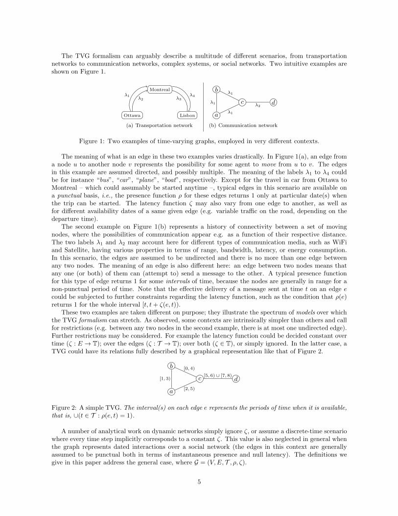
The TVG formalism can arguably describe a multitude of different scenarios, from transportationnetworks to communication networks, complex systems, or social networks. Two intuitive examples areshown on Figure 1.

Ottawa

Montreal

Lisbon

λ1λ2 λ3

λ4

(a) Transportation network

a

b

c dλ1

λ1

λ1

λ2

(b) Communication network

Figure 1: Two examples of time-varying graphs, employed in very different contexts.

The meaning of what is an edge in these two examples varies drastically. In Figure 1(a), an edge froma node u to another node v represents the possibility for some agent to move from u to v. The edgesin this example are assumed directed, and possibly multiple. The meaning of the labels λ1 to λ4 couldbe for instance “bus”, “car”, “plane”, “boat”, respectively. Except for the travel in car from Ottawa toMontreal – which could assumably be started anytime –, typical edges in this scenario are available ona punctual basis, i.e., the presence function ρ for these edges returns 1 only at particular date(s) whenthe trip can be started. The latency function ζ may also vary from one edge to another, as well asfor different availability dates of a same given edge (e.g. variable traffic on the road, depending on thedeparture time).

The second example on Figure 1(b) represents a history of connectivity between a set of movingnodes, where the possibilities of communication appear e.g. as a function of their respective distance.The two labels λ1 and λ2 may account here for different types of communication media, such as WiFiand Satellite, having various properties in terms of range, bandwidth, latency, or energy consumption.In this scenario, the edges are assumed to be undirected and there is no more than one edge betweenany two nodes. The meaning of an edge is also different here: an edge between two nodes means thatany one (or both) of them can (attempt to) send a message to the other. A typical presence functionfor this type of edge returns 1 for some intervals of time, because the nodes are generally in range for anon-punctual period of time. Note that the effective delivery of a message sent at time t on an edge ecould be subjected to further constraints regarding the latency function, such as the condition that ρ(e)returns 1 for the whole interval [t, t+ ζ(e, t)).

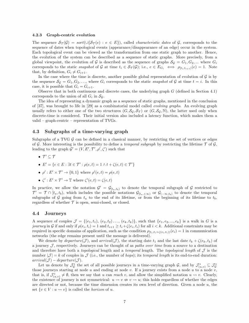
These two examples are taken different on purpose; they illustrate the spectrum of models over whichthe TVG formalism can stretch. As observed, some contexts are intrinsically simpler than others and callfor restrictions (e.g. between any two nodes in the second example, there is at most one undirected edge).Further restrictions may be considered. For example the latency function could be decided constant overtime (ζ : E → T); over the edges (ζ : T → T); over both (ζ ∈ T), or simply ignored. In the latter case, aTVG could have its relations fully described by a graphical representation like that of Figure 2.

a

b

c d[1, 3)

[2, 5)

[0, 4)

[5, 6) ∪ [7, 8)

Figure 2: A simple TVG. The interval(s) on each edge e represents the periods of time when it is available,that is, ∪(t ∈ T : ρ(e, t) = 1).

A number of analytical work on dynamic networks simply ignore ζ, or assume a discrete-time scenariowhere every time step implicitly corresponds to a constant ζ. This value is also neglected in general whenthe graph represents dated interactions over a social network (the edges in this context are generallyassumed to be punctual both in terms of instantaneous presence and null latency). The definitions wegive in this paper address the general case, where G = (V,E, T , ρ, ζ).

5

4 Definitions of TVG concepts

This section transposes and generalizes a number of dynamic network concepts into the framework oftime-varying graphs. A majority of them emerged independently in various areas of scientific literature;some appeared more specifically; some others are original propositions.

4.1 The underlying graph G

Given a TVG G = (V,E, T , ρ, ζ), the graph G = (V,E) is called underlying graph of G. This static graphshould be seen as a sort of footprint of G, which flattens the time dimension and indicates only the pairsof nodes that have relations at some time in T . It is a central concept that is used recurrently in thefollowing.

In most studies and applications, G is assumed to be connected; in general, this is not necessarily thecase. Let us stress that the connectivity of G = (V,E) does not imply that G is connected at a giventime instant; in fact, G could be disconnected at all times. The lack of relationship, with regards toconnectivity, between G and its footprint G is even stronger: the fact that G = (V,E) is connected doesnot even imply that G is “connected over time”, as illustrated on Figure 3.

a

b cd

[0, 1)[2, 3)

[0, 1)

Figure 3: An example of TVG that is not “connected over time”, although its underlying graph G isconnected. Here, the nodes a and d have no mean to reach each other through a chain of interaction.

4.2 Point of views

Depending on the problem under consideration, it may be convenient to look at the evolution of thesystem from the point of view of a given relation (edge), a given entity (node), or from that of theglobal system (entire graph). We respectively qualify these views as edge-centric, vertex-centric, andgraph-centric.

4.2.1 Edge-centric evolution

From an edge standpoint, the notion of evolution comes down to a variation of availability and latencyover time. We define the available dates of an edge e, noted I(e), as the union of all dates at which the edgeis available, that is, I(e) = {t ∈ T : ρ(e, t) = 1}. When I(e) is expressed as a multi-interval of availabilityI(e) = {[t1, t2)∪ [t3, t4)...}, where ti < ti+1, the sequence of dates t1, t3, ... is called appearance dates of e,noted App(e), and the sequence of dates t2, t4, ... is called disappearance dates of e, noted Dis(e). Finally,the sequence t1, t2, t3, ... is called characteristic dates of e, noted ST (e). In the following, we use thenotation ρ[t,t′)(e) = 1 to indicate that ∀t′′ ∈ [t, t′), ρ(e, t′′) = 1.

4.2.2 Vertex-centric evolution

From a node standpoint, the evolution of the network materializes as a succession of changes amongits neighborhood. This point of view does not appear frequently in the literature; yet, it was used forexample in [59] to express dynamic properties in terms of local variation of the sequence of neighborhoodsNt1(v), Nt2(v).. where Nt(v) denotes the neighbors of v at time t and each ti corresponds to a date oflocal change (i.e., appearance/disappearance of an incident edge).

The degree of a node u can be defined both in punctual or integral terms, e.g. with Degt(u) = |Et(u)|,or DegT (u) = | ∪ {Et(u) : t ∈ T }| where Et(u) indicates the set of edges incident on u at time t.

6

4.2.3 Graph-centric evolution

The sequence ST (G) = sort(∪{ST (e) : e ∈ E}), called characteristic dates of G, corresponds to thesequence of dates when topological events (appearance/disappearance of an edge) occur in the system.Each topological event can be viewed as the transformation from one static graph to another. Hence,the evolution of the system can be described as a sequence of static graphs. More precisely, from aglobal viewpoint, the evolution of G is described as the sequence of graphs SG = G1, G2, ... where Gicorresponds to the static snapshot of G at time ti ∈ ST (G); i.e., e ∈ EGi

⇐⇒ ρ[ti,ti+1)(e) = 1. Notethat, by definition, Gi 6= Gi+1.

In the case where the time is discrete, another possible global representation of evolution of G is bythe sequence SG = G1, G2, . . ., where Gi corresponds to the static snapshot of G at time t = i. In thiscase, it is possible that Gi = Gi+1.

Observe that in both continuous and discrete cases, the underlying graph G (defined in Section 4.1)corresponds to the union of all Gi in SG .

The idea of representing a dynamic graph as a sequence of static graphs, mentioned in the conclusionof [37], was brought to life in [29] as a combinatorial model called evolving graphs. An evolving graphusually refers to either one of the two structures (G,SG ,ST ) or (G,SG ,N), the latter used only whendiscrete-time is considered. Their initial version also included a latency function, which makes them avalid – graph-centric – representation of TVGs.

4.3 Subgraphs of a time-varying graph

Subgraphs of a TVG G can be defined in a classical manner, by restricting the set of vertices or edgesof G. More interesting is the possibility to define a temporal subgraph by restricting the lifetime T of G,leading to the graph G′ = (V,E′, T ′, ρ′, ζ ′) such that

• T ′ ⊆ T

• E′ = {e ∈ E : ∃t ∈ T ′ : ρ(e, t) = 1 ∧ t+ ζ(e, t) ∈ T ′}

• ρ′ : E′ × T ′ → {0, 1} where ρ′(e, t) = ρ(e, t)

• ζ ′ : E′ × T ′ → T where ζ ′(e, t) = ζ(e, t)

In practice, we allow the notation G′ = G[ta,tb) to denote the temporal subgraph of G restricted toT ′ = T ∩ [ta, tb), which includes the possible notations G[ta,+∞) or G(−∞,tb) to denote the temporalsubgraphs of G going from ta to the end of its lifetime, or from the beginning of its lifetime to tb,regardless of whether T is open, semi-closed, or closed.

4.4 Journeys

A sequence of couples J = {(e1, t1), (e2, t2) . . . , (ek, tk)}, such that {e1, e2, ..., ek} is a walk in G is ajourney in G if and only if ρ(ei, ti) = 1 and ti+1 ≥ ti+ζ(ei, ti) for all i < k. Additional constraints may berequired in specific domains of application, such as the condition ρ[ti,ti+ζ(ei,ti))(ei) = 1 in communicationnetworks (the edge remains present until the message is delivered).

We denote by departure(J ), and arrival(J ), the starting date t1 and the last date tk + ζ(ek, tk) ofa journey J , respectively. Journeys can be thought of as paths over time from a source to a destinationand therefore have both a topological length and a temporal length. The topological length of J is thenumber |J | = k of couples in J (i.e., the number of hops); its temporal length is its end-to-end duration:arrival(J )− departure(J ).

Let us denote by J ∗G the set of all possible journeys in a time-varying graph G, and by J ∗(u,v) ⊆ J∗G

those journeys starting at node u and ending at node v. If a journey exists from a node u to a node v,that is, if J ∗(u,v) 6= ∅, then we say that u can reach v, and allow the simplified notation u v. Clearly,the existence of journey is not symmetrical: u v < v u; this holds regardless of whether the edgesare directed or not, because the time dimension creates its own level of direction. Given a node u, theset {v ∈ V : u v} is called the horizon of u.

7

4.5 Distance

As observed, the length of a journey can be measured both in terms of hops or time. This gives rise totwo distinct definitions of distance in a time-varying graph G:

• The topological distance from a node u to a node v at time t, noted du,t(v), is defined as Min{|J | :J ∈ J ∗(u,v), departure(J ) ≥ t}. For a given date t, a journey whose departure is t′ ≥ t and

topological length is equal to du,t(v) is qualified as shortest ;

• The temporal distance from u to v at time t, noted du,t(v) is defined as Min{arrival(J ) : J ∈J ∗(u,v), departure(J ) ≥ t} − t. Given a date t, a journey whose departure is t′ ≥ t and arrival is

t + du,t(v) is qualified as foremost. Finally, for any given date t, a journey whose departure is ≥ t

and temporal length is Min{du,t′(v) : t′ ∈ T ∩ [t,+∞)} is qualified as fastest.

The problem of computing shortest, fastest, and foremost journeys in delay-tolerant networks wasintroduced in [15], and an algorithm for each of the three metrics was provided for the centralized versionof the problem (assuming complete knowledge of G). Temporal distance and related concepts have beenpractically used in various fields ranging from social network analysis [67] to warning delivery protocolsin vehicular networks [63].

A concept closely related to that of temporal distance is that of temporal view, introduced in [49] inthe context of social network analysis. The temporal view1 that a node v has of another node u at timet, denoted φv,t(u), is defined as the latest (i.e., largest) t′ ≤ t at which a message received by time t at vcould have been emitted at u; that is, in our formalism,

φv,t(u) = Max{departure(J ) : J ∈ J ∗(u,v), arrival(J ) ≤ t}.

The question of knowing whether all the nodes of a network could know their temporal views in realtime was recently answered (affirmatively) in [21].

4.6 Other temporal concepts

The number of definitions built on top of temporal concepts could grow endlessly, and our aim is certainlynot to enumerate all of them. Yet, here is a short list of additional concepts that we believe are generalenough to be possibly useful in several analytical contexts.

The concept of eccentricity can be separated into a topological eccentricity and a temporal eccentricity,following the same mechanism as for the concept of distance. The temporal eccentricity of a node u attime t, εt(u), is defined as max{du,t(v) : v ∈ V }, that is, the duration of the “longest” foremost journeyfrom u to any other node. The concept of diameter can similarly be separated into those of topologicaldiameter and temporal diameter, the latter being defined at time t as max{εt(u) : u ∈ V }. These temporalversions of eccentricity and diameter were proposed in [15] for the case that the reference time t is theinitial time t0 of the system. The temporal diameter was further investigated from a stochastic point ofview by Chaintreau et al. in [23].

Clementi et al. introduced in [25] a concept of dynamic expansion – the dynamic counterpart ofthe concept of node expansion in static graphs – which accounts for the maximal speed of informationpropagation. Given a subset of nodes V ′ ⊆ V , and two dates t1, t2 ∈ T , the dynamic expansion of V ′

from time t1 to time t2 is the size of the set {v ∈ V rV ′ : ∃J(u,v) ∈ J ∗G[t1,t2) : u ∈ V ′}, that is, in a sense,

the collective horizon of V ′ in G[t1,t2).The concept of journey was dissociated in [21] into direct and indirect journeys. A journey J =

{(e1, t1), (e2, t2) . . . , (ek, tk)} is said direct iff ∀i, 1 ≤ i < k, ρ(ei+1, ti + ζ(ei, ti)) = 1, that is, everynext edge in J is directly available; it is said indirect otherwise. The knowledge of whether a journey isdirect or indirect was directly exploited by the distributed algorithm in [21] to compute temporal distancesbetween nodes. Such a parameter could also play a role in the context of delay-tolerant routing, indicatingwhether a store-carry-forward mechanism is required (for indirect journeys).

1This concept was called simply “view” in [49]; since the term view has a very different meaning in distributed computing(e.g., [71]), the adjective “temporal” has been added to avoid confusion.

8

5 TVG Classes

In this section we discuss the impact of properties of TVGs on the feasibility and complexity of distributedproblems, reviewing and unifying existing works from the literature. In particular, we identify a hierarchyof classes of TVGs based on temporal properties that are formulated using the concepts presented in theprevious section. These class-defining properties, organized in an ascending order of assumptions – frommore general to more specific, are important in that they imply necessary conditions and impossibilityresults for distributed computations.

Let us start with the simplest Class.

Class 1 ∃u ∈ V : ∀v ∈ V, u v.

That is, at least one node can reach all the others. This condition is necessary, for example, for broadcastto be feasible from at least one node.

Class 2 ∃u ∈ V : ∀v ∈ V, v u.

That is, at least one node can be reached by all the others. This condition is necessary to be able tocompute a function whose input is spread over all the nodes, with at least one node capable of generatingthe output. Any algorithm for which a terminal state must be causally related to all the nodes initialstates also falls in this category, such as leader election in anonymous networks or counting the numberof nodes.

Class 3 (Connectivity over time): ∀u, v ∈ V, u v.

That is, every node can reach all the others; in other words, the TVG is connected over time. By thesame discussions as for Class 1 and Class 2, this condition is necessary to enable broadcast from anynode, to compute a function whose output is known by all the nodes, or to ensure that every node has achance to be elected.

These three basic classes were used e.g. in [19] to investigate how relations between TVGs propertiesand feasibility of algorithms could be formally established, based on a combination of evolving graphs [29]and graph relabelings [56]. Variants of these classes can be found in recent literature, e.g. in [33] wherethe assumption that connectivity over time eventually takes place among a stable subset of the nodes isused to implement failure detectors in dynamic networks.

Class 4 (Round connectivity): ∀u, v ∈ V,∃J1 ∈ J ∗(u,v),∃J2 ∈ J∗(v,u) : arrival(J1) ≤ departure(J2).

That is, every node can reach all the others and be reached back afterwards. Such a condition may berequired e.g. for adding explicit termination to broadcast, election, or counting algorithms.

The classes defined so far are in general relevant in the case that the lifetime is finite and a limitednumber of topological events are considered. When the lifetime is infinite, connectivity over time isgenerally assumed on a regular basis, and more elaborated assumptions can be considered.

Class 5 (Recurrent connectivity): ∀u, v ∈ V,∀t ∈ T ,∃J ∈ J ∗(u,v) : departure(J ) > t.

That is, at any point t in time, the temporal subgraph G[t,+∞) remains connected over time. This class isimplicitly considered in most works on delay-tolerant networks. It indeed represents those DTNs whererouting can always be achieved over time. This class was referred to as eventually connected networks byAwerbuch and Even in [5], although the terminological compound “eventually connected” was also usedwith different meaning in the recent literature (which we mention in another definition below).

As discussed in Section 4.1, the fact that the underlying graph G = (V,E) is connected does notimply that G is connected over time – the ordering of topological events matters. Such a condition ishowever necessary to allow connectivity over time and thus to perform any type of global computation.Therefore, the following three classes explicitly assume that the underlying graph G is connected.

Class 6 (Recurrence of edges): ∀e ∈ E,∀t ∈ T ,∃t′ > t : ρ(e, t′) = 1 and G is connected.

9

That is, if an edge appears once, it appears infinitely often. Since the underlying graph G is connected,we have Class 6 ⊆ Class 5. Indeed, if all the edges of a connected graph appear infinitely often, thenthere must exist, by transitivity, a journey between any pairs of nodes infinitely often.

In a context where connectivity is recurrently achieved, it becomes interesting to look at problemswhere more specific properties of the journeys are involved, e.g. the possibility to broadcast a piece ofinformation in a shortest, foremost, or fastest manner (see Section 4.5 for definitions). Interestingly, thesethree declinations of the same problem have different requirements in terms of TVG properties. It is forexample possible to broadcast in a foremost fashion in Class 6, whereas shortest and fastest broadcastsare not possible [20].

Shortest broadcast becomes however possible if the recurrence of edges is bounded in time, and thebound known to the nodes, a property characterizing the next class:

Class 7 (Time-bounded recurrence of edges): ∀e ∈ E,∀t ∈ T ,∃t′ ∈ [t, t+∆), ρ(e, t′) = 1, for some ∆ ∈ Tand G is connected.

Some implications of this class include a temporal diameter that is bounded by ∆Diam(G), as wellas the possibility for the nodes to wait a period of ∆ to discover all their neighbors (if ∆ is known).The feasibility of shortest broadcast follows naturally by using a ∆-rounded breadth-first strategy thatminimizes the topological length of journeys.

A particular important type of bounded recurrence is the periodic case:

Class 8 (Periodicity of edges): ∀e ∈ E,∀t ∈ T ,∀k ∈ N, ρ(e, t) = ρ(e, t + kp), for some p ∈ T and G isconnected.

The periodicity assumption holds in practice in many cases, including networks whose entities are mobilewith periodic movements (satellites, guards tour, subways, or buses). The periodic assumption withina delay-tolerant network has been considered, among others, in the contexts of network exploration [31,40, 30] and routing [48, 57]. Periodicity enables also the construction of foremost broadcast trees thatcan be re-used (modulo p in time) for subsequent broadcasts [21] (whereas the more general classes ofrecurrence requires the use of a different tree for every foremost broadcast).

More generally, the point in exploiting TVG properties is to rely on invariants that are generatedby the dynamics (e.g. recurrent existence of journeys, periodic optimality of a broadcast tree, etc.). Insome works, particular assumptions on the network dynamics are made to obtain invariants of a moreclassical nature. Below are some examples of classes, formulated using the graph-centric point of view of(discrete-time) evolving graphs, i.e., where G = (G,SG ,N).

Class 9 (Constant connectivity): ∀Gi ∈ SG , Gi is connected.

Here, the dynamics of the network is not constrained as long as it remains connected in every time step.Such a class was used for example in [59] to enable progression hypotheses on the broadcast problem.Indeed, if the network is always connected, then at every time step there must exist an edge between aninformed node and a non-informed node, which allows to bound broadcast time by n = |V | time steps(worst case scenario). This class was also considered in [52] for the problem of consensus.

Class 10 (T-interval connectivity): ∀i ∈ N, T ∈ N,∃G′ ⊆ G : VG′ = VG, G′ is connected, and ∀j ∈

[i, i+ T − 1), G′ ⊆ Gj.

This class is a particular case of constant connectivity in which a same spanning connected subgraph ofthe underlying graph G is available for any period of T consecutive time steps. It was introduced in [51]to study problems such as counting, token dissemination, and computation of functions whose input isspread over all the nodes (considering an adversarial edge schedule). The authors show that computationcould be sped up of a factor T compared to the 1-interval connected graphs, that is, graphs of Class 9.

Other classes of TVGs can be found in [62], based on intermediate properties between constantconnectivity and connectivity over time. They include Class 11 and Class 12 below.

10

C4 C3C2

C1C5

C6

C13

C7C8

C12C11C9C10

Figure 4: Relations of inclusion between classes (from specific to general).

Class 11 (Eventual instant-connectivity): ∀i ∈ N,∃j ∈ N : j ≥ i, Gj is connected. In other words, thereis always a future time step in which the network is instantly connected.

This class was simply referred to as eventual connectivity in [62], but since the meaning is differentthan that of [5] (connectivity over time), we renamed it to avoid ambiguities.

Class 12 (Eventual instant-routability): ∀u, v ∈ V,∀i ∈ N,∃j ∈ N : j ≥ i and a path from u to v existsin Gj.

That is, for any two nodes, there is always a future time step in which a instant path exists betweenthem. The difference with Class 11 is that these paths may occur at different times for different pairs ofnodes. Classes 11 and 12 were used in [62] to represent networks where routing protocols for (connected)mobile ad hoc networks eventually succeed if they tolerate transient topological faults.

Most of the works listed above strove to characterize the impact of various temporal properties onproblems or algorithms. A reverse approach was considered by Angluin et al. in the field of populationprotocols [2, 3], where for a given assumption (that any pair of node interacts infinitely often), theycharacterized all the problems that could be solved in this context. The corresponding class is generallyreferred to as that of (complete) graph of interaction.

Class 13 (Complete graph of interaction): The underlying graph G=(V,E) is complete, and ∀e ∈ E,∀t ∈T ,∃t′ > t : ρ(e, t′)=1.

From a time-varying graph perspective, this class is the specific subset of Class 6, in which the underlyinggraph G is complete. Various types of schedulers and assumptions have been subsequently consideredin the field of population protocols, adding further constraints to Class 13 (e.g. weak fairness, strongfairness, bounded, or k-bounded schedulers) as well as interaction graphs which might not be complete.

An interesting aspect of unifying these properties within the same formalism is the possibility to seehow they relate to one another, and to compare the associated solutions or algorithms. An insight forexample can be gained by looking at the short classification shown in Figure 4, where basic relations ofinclusion between the above classes are reported. These inclusion are strict: for each relation, the parentclass contains some time-varying graphs that are not in the child class.

Clearly, one should try to solve a problem in the most general context possible. The right-most classesare so general that they offer little properties to be exploited by an algorithm, but some intermediateclasses, such as Class 5, appear quite central in the hierarchy. This class indeed contains all the classeswhere significant work was done. A problem solved in this class would therefore apply to virtually all thecontexts considered heretofor in the literature.

Such a classification may also be used to categorize problems themselves. As mentioned above, shortestbroadcast is not generally achievable in Class 6, whereas foremost broadcast is. Similarly, it was shownin [20] that fastest broadcast is not feasible in Class 7, whereas shortest broadcast can be achieved withsome knowledge. Since Class 7 ⊂ Class 6, we have

foremostBcast � shortestBcast � fastestBcast

where � is a partial order on these problems topological requirements.

11

6 TVG and Network Analysis

This section is concerned with the a posteriori analysis of network traces. We discuss three particularaspects of this general question, which are i) how network traces could be checked for inclusion in some ofthe above classes, ii) how temporal concepts can be leveraged to express new phenomenon or propertiesin complex systems, and iii) how TVGs could be used to study a coarser-grain evolution of networkproperties, whether these properties are of a classical or a temporal nature (which implies differentapproaches).

6.1 Recognizing TVGs

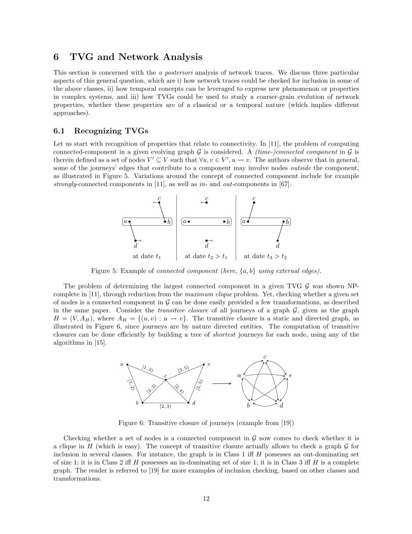
Let us start with recognition of properties that relate to connectivity. In [11], the problem of computingconnected-component in a given evolving graph G is considered. A (time-)connected component in G istherein defined as a set of nodes V ′ ⊆ V such that ∀u, v ∈ V ′, u v. The authors observe that in general,some of the journeys’ edges that contribute to a component may involve nodes outside the component,as illustrated in Figure 5. Variations around the concept of connected component include for examplestrongly-connected components in [11], as well as in- and out-components in [67].

a b

c

d

a b

c

d

a b

c

d

at date t1 at date t2 > t1 at date t3 > t2

Figure 5: Example of connected component (here, {a, b} using external edges).

The problem of determining the largest connected component in a given TVG G was shown NP-complete in [11], through reduction from the maximum clique problem. Yet, checking whether a given setof nodes is a connected component in G can be done easily provided a few transformations, as describedin the same paper. Consider the transitive closure of all journeys of a graph G, given as the graphH = (V,AH), where AH = {(u, v) : u v}. The transitive closure is a static and directed graph, asillustrated in Figure 6, since journeys are by nature directed entities. The computation of transitiveclosures can be done efficiently by building a tree of shortest journeys for each node, using any of thealgorithms in [15].

a

b

c

d

e

[1, 2

)

[2, 3)

[3, 5

)

[1, 2)

[2, 3) [2, 4)

[3,5)

a

b

c

d

e

Figure 6: Transitive closure of journeys (example from [19])

Checking whether a set of nodes is a connected component in G now comes to check whether it isa clique in H (which is easy). The concept of transitive closure actually allows to check a graph G forinclusion in several classes. For instance, the graph is in Class 1 iff H possesses an out-dominating setof size 1; it is in Class 2 iff H possesses an in-dominating set of size 1; it is in Class 3 iff H is a completegraph. The reader is referred to [19] for more examples of inclusion checking, based on other classes andtransformations.

12

6.2 Transposing the definition of phenomena

The following paragraphs discuss the possible use of TVGs to express the redefinition (or translation) ofusual concepts in complex system analysis, into a dynamic version. We provide two examples: the smallworld effect, and the fairness in a network. Further examples could certainly be found.

6.2.1 Small World

A small-world network is one where the distance between two randomly chosen nodes (in terms of hops)grows logarithmically with the number of nodes in the network. Time-varying graph concepts, such asthose of journeys, connectivity over time, and temporal distance have been used in [69] to characterizethe small world behavior of real-world networks in temporal terms, that is, the fact that there is alwaysa journey of short duration between any two nodes. Among the concepts introduced in [69] is thecharacteristic temporal path length, defined as∑

u,v∈V dt0 (u,v)

|V 2|

where t0 is the first date in the network lifetime T . In other words, this value is the average of temporaldistances between all pairs of nodes at starting time. An average of this value over the network lifetimewould certainly be meaningful as well.

As per the topological meaning (i.e., in terms of hops) of the small world property in a dynamiccontext, e.g. the fact that “mobile networks have a diameter of 7” [60], it could be formalized as follows:

∀u, v ∈ V,∀t ∈ T ,∃J ∈ J ∗(u,v) : departure(J ) ≥ t, |J | ≤ 7.

6.2.2 Fairness and Balance

Other properties of interest can take the form of quantities or statistical information. Consider thecaricatural example of Figure 7, where nodes a to f represent individuals, each of which meets someother individuals every week (on a periodical basis).

a b c d e fMonday Tuesday Wednesday Thursday Friday

Figure 7: Weekly interactions between six people.

A glance at the structure of this network does not reveal any strong anomaly: a) the graph is a line,b) its diameter is 5, c) nodes c and d are more central than the other nodes, etc. However, if we considerthe temporal dimension of this graph, it appears that (the interaction described by) the graph is highlyunfair and asymmetric: any information originating from a can reach f within 5 to 11 days (dependingon what day it is originated), whereas information from f needs about one month to reach a. Node aalso appears more central than c and d from a temporal point of view.

We could define here a concept of fairness as being the standard deviation among the nodes temporaleccentricities (see Section 4.6). This indicator provides an outline on how well the interactions arebalanced among nodes. For instance, the TVG of Figure 7 is highly unfair; while the one shown inFigure 8 is fairer (still, the fairness remains strucurally constrained by G, the underlying graph).

a b c d e fMonday Thursday Monday Thursday Monday

Figure 8: Weekly interactions between six people - Fairer version.

A related measure could reflect how balanced the graph is with respect to the time dimension, sincethe metrics of interest are time-dependent (e.g. the temporal diameter of the TVG in Figure 8 is much

13

lower on Mondays than on Tuesdays). Recent efforts in similar directions include measuring the temporaldistance between individuals based on e-mail datasets [49, 50] or inter-meeting times [69], or the redefi-nition of further concepts built on top of temporal distance, such as temporal betweenness and temporalcloseness [68].

6.3 Capturing the coarse-grain evolution

At many occasions in this paper, we have focused on the question of how static concepts translate into adynamic context, e.g. through the redefinition of more basic notions like those of paths (into journeys),distance (into temporal distance) or connectivity (into connectivity over time). From a complex systemperspective, these temporal indicators, as well as those built on top of them, are completing the set ofatemporal indicators usually considered, such as (the normal versions of) distance and diameter, density,clustering coefficient, or modularity, to name a few. It is important to keep in mind that all theseindicators, whether temporal or atemporal, essentially accounts for network properties at a reasonablyshort time-scale (fine-grain dynamics). They do not reflect how network evolves over longer periods oftime (coarse-grain dynamics).

We present below a general approach to look at the evolution of both atemporal and temporal indi-cators [64]. Looking at the evolution of atemporal indicators can be done by representing the evolutionof the network as a sequence of static graphs, each of which represents the aggregated interactions overa given time-window. The usual indicators can then be normally measured on these graphs and theirevolution studied over time. The case of temporal indicators is more complex because the correspondingevaluation cannot be done on static graphs. The proposed solution is therefore to look at the evolutionof temporal indicators through a sequence of shorter (and non-aggregated) time-varying graphs, i.e., asequence of temporal subgraphs of the original time-varying graph that cover successive time-windows.

6.3.1 Evolution of Atemporal Indicators

TVGs as a sequence of footprints Given a TVG G = (V,E, T , ρ, ζ), one can define the footprint ofthis graph from t1 to t2 as the static graph G[t1,t2) = (V,E[t1,t2)) such that ∀e ∈ E, e ∈ E[t1,t2) ⇐⇒ ∃t ∈[t1, t2), ρ(e, t) = 1. In other words, the footprint aggregates all interactions of given time windows intostatic graphs. Let the lifetime T of the time-varying graph be partitioned in consecutive sub-intervalsτ = [t0, t1), [t1, t2) . . . [ti, ti+1), . . .; where each [tk, tk+1) can be noted τk. We call sequence of footprintsof G according to τ the sequence SF(τ) = Gτ0 , Gτ1 , . . .. Considering this sequence with a sufficient sizeof the intervals allows to overcome the strong fluctuations of fine-grain interactions, and focus insteadon more general trends of evolution. Note that the same approach could be considered with a sequenceof intervals that are overlapping (i.e., a sliding time-window) instead of disjoint ones. Another variationmay be considered based on whether the set of nodes in each Gτi is also allowed to vary. Since every graphin the sequence is static, any classical network parameter can be directly measured on it. Depending onthe parameter and on the application, different choices of granularity are more appropriate to capturea meaningful behavior. At one extreme, each interval could correspond to the smallest time unit (indiscrete-time systems), or to the time between any two consecutive modification of the graph; in thesecases the whole sequence becomes equivalent to the model of evolving graph [29]. At the other side of thespectrum, i.e. taking τ = T , the sequence would consist of a single footprint aggregating all interactionsover the network lifetime, that is, be equal to G, the underlying graph of G.

Looking at the evolution of atemporal parameters allows to understand how some emerging phenom-ena occur on the network structure, for instance, the densification of transportation networks (throughdiameter or average distance indicators), or the formation of communities in social networks (throughmodularity [12], cohesion [32] or other indicators e.g. [1, 14]).

6.3.2 Evolution of Temporal Indicators

Most temporal concepts – including those mentioned in Section 4 – are based on replacing the notionof path by that of journey. As a result, they can be declined into three versions depending on the type

14

of metric considered (i.e., shortest, foremost, fastest). Since journeys are paths over time, the evolutionof parameters based on journeys cannot be studied using a sequence of aggregated static graphs. Forexample, there might be a path between x and y in all footprints, and yet possibly no journey betweenthem depending on the precise chronology of interaction. Analyzing the evolution of such parametersrequires more than a sequence of static graphs.

TVGs as a sequence of (shorter) TVGs Temporal subgraphs have been defined in Section 4.Roughly speaking, they are themselves TVGs that reproduce all the interactions present in the originalTVG for a given time window – without aggregating them. In the same way as for the sequence offootprints, we can now look at the evolution of a TVG through a sequence of shorter TVGs ST(τ) =Gτ0 ,Gτ1 , . . ., in which the intervals are either disjoint or overlapping. Looking at the coarse-grain evolutionof temporal indicators could allow to answer questions like: how does the temporal distance between nodesevolve over time? Or more generally how a network self-organizes, optimizes, or deteriorate, in termsof temporal efficiency. Using concepts like the fairness, defined above, this may also help capture theemergence of non-apparent inequalities in a social network.

7 Random TVGs

Randomness in time-varying graphs can be introduced at several different levels. The most direct one isclearly that provided by probabilistic time-varying graphs, where the presence function ρ : E ×T → [0, 1]indicates the probability that a given edge is available at a given time. In a context of mobility, theprobability distribution of ρ is intrinsically related to the expected mobility of the nodes. Popularexample of random mobility models include the Random Waypoint and Random Direction models [17],where waypoints of consecutive movements are chosen uniformly at random. Mobility models fromsocial networks include the Time-Variant Community model (TVC) [39], and the more recent Home-cellCommunity-based Mobility Model (HCMM) [13].

Definitions of random TVG differ depending on whether the time is discrete or continuous.A (discrete-time) random time-varying graph is a TVG whose lifetime is an interval of N and whose

sequence of characteristic graphs SG = G1, G2, .. is such that every Gi is a Erdos and Renyi randomgraph; that is, ∀e ∈ V 2,P[e ∈ EGi ] = p for some p; this definition is introduced by Chaintreau et al. [23].

One particularity of discrete-time random TVGs is that the Gis are independent with respect to eachother. While this definition allows purely random graphs, it does not capture some properties of realworld networks, such as the fact that an edge may be more likely to be present in Gi+1 if it is alreadypresent in Gi. This question is addressed by Clementi et al. [24] by introducing Edge-Markovian EvolvingGraphs. These are discrete-time evolving graphs in which the presence of every edge follows an individualMarkovian process. More precisely, the sequence of characteristic graph SG = G1, G2, .. is such that{

P[e ∈ EGi+1 |e /∈ EGi ] = p

P[e /∈ EGi+1|e ∈ EGi

] = q

for some p and q called birth rate and death rate, respectively. The probability that a given edge remainsabsent or present from Gi to Gi+1 is obtained by complement of p and q. The very idea of considering aMarkovian Evolving Graph seems to have appeared in [4], in which the authors consider a particular casethat is substantially equivalent to the discrete-time random TVG from [23]. Variations around the modelof edge-markovian evolving graphs include cases where Gi+1 depends not only on Gi, but also on oldergraphs Gi−1, Gi−2,... (the edges follow a higher order Markovian process) [34]. Edge-Markovian EGswere used in [24], along with the concept of dynamic expansion (see Section 4.6) to address stochasticquestions such as does dynamics necessarily slow down a broadcast? Or can random node mobility beexploited to speed-up information spreading? Baumann et al. extended this work in [9] by establishingtight bounds on the propagation time for any birth and death rates.

A continuous-time random time-varying graph is a TVG in which the appearance of every edge obeysa Poisson process, that is, ∀e ∈ V 2,∀ti ∈ App(e),P[ti+1 − ti < d] = λeλx for some λ; this definition is

15

introduced by Chaintreau et al. in [23].2

Random time-varying graphs, both discrete-time and continuous-time, were used in [23] to characterizephase transitions between no-connectivity and connectivity over time as a function of the number of nodes,a given time-window duration, and constraints on both the topological and temporal lengths of journeys.

8 Research Problems and Directions

The first most obvious research task is that of exploring the universe of dynamic networks using theformal tools provided by the TVG formalism. The long-term goal is that of providing a comprehensivemap of this universe, identifying both the commonality and the natural differences between the varioustypes of dynamical systems modeled by TVG. Additionally, several, more specific research areas can beidentified including the ones described below.

Distributed TVG algorithms design and analysis. The design and analysis of distributed algorithmsand protocols for time-varying graphs is an open research area. In fact very few problems have beenattacked so far: routing and broadcasting in delay-tolerant networks; broadcasting and exploration inopportunistic-mobility networks; new self-stabilization techniques (such as the one in [44]); detection ofemergence and resilience of communities, and viral marketing in social networks.

Design and optimization of TVG. If the interactions in a network can be planned – decided by adesigner –, then a number of new interesting optimization problems arise with the design of time-varyinggraph. They may concern for example the minimization of the temporal diameter or the balancingof nodes eccentricities. E.g. how to modify the days of meeting in Figure 7 so as to minimize thenetwork diameter (still preventing two meetings the same day for each people)? Figure 8 showed a basicimprovement (the diameter was between 24 and 30 days, and shortened to between 14 and 20 days). Isa given setting optimal? How to prove it? What if the underlying graph can also be modified? etc. Awhole field is opening that promizes exciting research avenues.

Complexity Analysis. Analyzing the complexity of a distributed algorithm in a TVG – e.g. in numberof messages – is not trivial, partly because contrarily to the static cases, the complexity of an algorithmin a dynamic network has a strong dependency, not only on the usual network parameters (number ofnodes, edges, etc.), but also on the number of topological events taking place during its execution. Inmany of the algorithms we have encountered, the majority of messages is in fact directly triggered bytopological events, e.g., in reaction to the local appearance or disappearance of an edge. The number oftopological events therefore represents a new complexity parameter, whose impact on various problemsremains to study.

Patterns Detection and Visualization. In order to better understand complex systems and theirdynamic aspects, data need to be visualized in a way that allows the intuition to guess a particularproperty or interaction pattern. Several works are progressing in this direction, including the Gephiproject [8] or the Graphstream library [26], where both nodes and edges can be specified with temporaland spatial attributes that enable the visualization of their evolution. These can be used to have a globalvision of the phenomena to be explained at the micro, meso and macro levels. In addition, throughthe use of the interaction-centric point view, TVGs enable to look at the interplay between topologicalaspects that allow local interaction to have global effects.

References

[1] J. I. Alvarez-Hamelin, L. Dall’Asta, A. Barrat, and A. Vespignani. K-core decomposition of internet graphs:hierarchies, self-similarity and measurement biases. Networks and Heterogeneous Media, 3(2):371–293, 2008.

[2] D. Angluin, J. Aspnes, Z. Diamadi, M. Fischer, and R. Peralta. Computation in networks of passively mobilefinite-state sensors. Distributed Computing, 18(4):235–253, 2006.

2It is interesting to note that in their definition of random TVG, the authors rely on a graph-centric point of view indiscrete time and on an edge-centric point of view in continuous time. The same trend can actually be observed in most ofthe works we reviewed here.

16

[3] D. Angluin, J. Aspnes, D. Eisenstat, and E. Ruppert. The computational power of population protocols.Distributed Computing, 20(4):279–304, 2007.

[4] C. Avin, M. Koucky, and Z. Lotker. How to explore a fast-changing world. In Proceedings of 35th InternationalColloquium on Automata, Languages and Programming (ICALP), pages 121–132, 2008.

[5] B. Awerbuch and S. Even. Efficient and reliable broadcast is achievable in an eventually connected network.In Proceedings of 3rd ACM symposium on Principles of Distributed Computing (PODC’84), pages 278–281,1984.

[6] L. Backstrom, D. Huttenlocher, J. Kleinberg, and X. Lan. Group formation in large social networks: member-ship, growth, and evolution. In Proceedings of 12th ACM International Conference on Knowledge Discoveryand Data Mining, pages 44–54, 2006.

[7] A. Balasubramanian, Y. Zhou, B. Croft, B.N. Levine, and A. Venkataramani. Web search from a bus. InProceedings of 2nd ACM Workshop on Challenged Networks (CHANTS), pages 59–66, 2007.

[8] M. Bastian, S. Heymann, and M. Jacomy. Gephi: An open source software for exploring and manipulatingnetworks. In Proceedings of 3rd International AAAI Conference on Weblogs and Social Media, 2009.

[9] H. Baumann, P. Crescenzi, and P. Fraigniaud. Parsimonious flooding in dynamic graphs. In Proceedings of28th ACM Symposium on Principles of Distributed Computing, pages 260–269, 2009.

[10] K.A. Berman. Vulnerability of scheduled networks and a generalization of Menger’s Theorem. Networks,28(3):125–134, 1996.

[11] S. Bhadra and A. Ferreira. Complexity of connected components in evolving graphs and the computationof multicast trees in dynamic networks. In Proceedings of 2nd International Conference on Ad Hoc, Mobileand Wireless Networks (AdHoc-Now), pages 259–270, 2003.

[12] V.D. Blondel, J.L. Guillaume, R. Lambiotte, and E. Lefebvre. Fast unfolding of communities in largenetworks. Journal of Statistical Mechanics: Theory and Experiment, 2008:P10008, 2008.

[13] C. Boldrini and A. Passarella. HCMM: Modelling spatial and temporal properties of human mobility drivenby users’ social relationships. Computer Communications, 33(9):1056–1074, 2010.

[14] K. Borne, S. Sanyal, and A.Vespignani. Network science. Annual Review of Information Science andTechnology, 41:537–607, 2007.

[15] B. Bui-Xuan, A. Ferreira, and A. Jarry. Computing shortest, fastest, and foremost journeys in dynamicnetworks. International Journal of Foundations of Comp. Science, 14(2):267–285, April 2003.

[16] J. Burgess, B. Gallagher, D. Jensen, and B.N. Levine. Maxprop: Routing for vehicle-based disruption-tolerant networks. In Proceedings of 25th IEEE Conference on Computer Communications (INFOCOM),pages 1–11, 2006.

[17] T. Camp, J. Boleng, and V. Davies. Diameter of the world-wide web. Wireless Communications and MobileComputing, 2(5):483 502, 2002.

[18] I. Cardei, C. Liu, and J. Wu. Routing in Wireless Networks with Intermittent Connectivity. In Encyclopediaof Wireless and Mobile Communications, CRC Press, Taylor & Francis, 2007.

[19] A. Casteigts, S. Chaumette, and A. Ferreira. Characterizing topological assumptions of distributed algo-rithms in dynamic networks. In Proceedings of 16th International Colloquium on Structural Information andCommunication Complexity (SIROCCO), pages 126–140, 2009. (Full version in arXiv:1102.5529.)

[20] A. Casteigts, P. Flocchini, B. Mans, and N. Santoro. Deterministic computations in time-varying graphs:Broadcasting under unstructured mobility. In Proceedings of 5th IFIP Conference on Theoretical ComputerScience (TCS), pages 111–124, 2010.

[21] A. Casteigts, P. Flocchini, B. Mans, and N. Santoro. Measuring temporal lags in delay-tolerant networks.In Proceedings of 25th IEEE International Parallel and Distributed Processing Symposium (IPDPS), 2011.

17

[22] A. Chaintreau, P. Hui, J. Crowcroft, C. Diot, R. Gass, and J. Scott. Impact of human mobility on oppor-tunistic forwarding algorithms. IEEE Transactions on Mobile Computing, 6(6):606–620, 2007.

[23] A. Chaintreau, A. Mtibaa, L. Massoulie, and C. Diot. The diameter of opportunistic mobile networks.Communications Surveys & Tutorials, 10(3):74–88, 2008.

[24] A. Clementi, C. Macci, A. Monti, F. Pasquale, and R. Silvestri. Flooding time in edge-markovian dynamicgraphs. In Proceedings of 27th ACM Symposium on Principles of Distributed Computing (PODC), pages213–222, 2008.

[25] A. Clementi and F. Pasquale. Information spreading in dynamic networks: An analytical approach. In: S.Nikoletseas, and J. Rolim (Eds), Theoretical Aspects of Distributed Computing in Sensor Networks, Springer,2010.

[26] A. Dutot, F. Guinand, D. Olivier, and Y. Pigne. Graphstream: A tool for bridging the gap between complexsystems and dynamic graphs. In Proceedings of of Emergent Properties in Natural and Artificial ComplexSystems. (EPNACS), pages 63–72, 2007.

[27] N. Eagle and A. (Sandy) Pentland. Reality mining: sensing complex social systems. Personal UbiquitousComput., 10(4):255–268, 2006.

[28] J. Eriksson, H. Balakrishnan, and S. Madden. Cabernet: Vehicular content delivery using WiFi. In Proceed-ings of 14th ACM/IEEE International Conference on Mobile Computing and Networking, pages 199–210,2008.

[29] A. Ferreira. Building a reference combinatorial model for MANETs. IEEE Network, 18(5):24–29, 2004.

[30] P. Flocchini, M. Kellett, P. Mason, and N. Santoro. Searching for black holes in subways. Theory ofComputing Systems, 50(1):158–184, 2012.

[31] P. Flocchini, B. Mans, and N. Santoro. Exploration of periodically varying graphs. In Proceedings of 20thInternational Symposium on Algorithms and Computation (ISAAC), pages 534–543, 2009.

[32] A Friggeri, G Chelius, and E Fleury. Ego-munities, Exploring Socially Cohesive Person-based Communities.Technical Report 7535, INRIA, 2011.

[33] F. Greve, L. Arantes, and P. Sens. What model and what conditions to implement unreliable failure detectorsin dynamic networks? In 3rd Workshop on Theoretical Aspects of Dynamic Distributed Systems (TADDS),2011.

[34] P. Grindrod and M. Parsons. Social networks: Evolving graphs with memory dependent edges. Technicalreport, MPS 2010-02, University of Reading, 2010.

[35] M. Grossglauser and M. Vetterli. Locating nodes with EASE: Last encounter routing in ad hoc networksthrough mobility diffusion. In Proceedings of 22nd Conference on Computer Communications (INFOCOM),volume 3, pages 1954–1964, 2003.

[36] S. Guo and S. Keshav. Fair and efficient scheduling in data ferrying networks. In Proceedings of ACMConference on Emerging Network Experiment and Technology, pages 1–13, 2007.

[37] F. Harary and G. Gupta. Dynamic graph models. Mathematical and Computer Modelling, 25(7):79–88, 1997.

[38] P. Holme. Network reachability of real-world contact sequences. Physical Review E, 71(4):46119, 2005.

[39] W. Hsu, T. Spyropoulos, K. Psounis, and A. Helmy. Modeling time-variant user mobility in wireless mobilenetworks. In Proceedings of 26th IEEE Conference on Computer Communications (INFOCOM), pages 758–766, 2007.

[40] D. Ilcinkas and A.M. Wade. On the power of waiting when exploring public transportation systems. InProceedings of 15th International Conference on Principles of Distributed Systems (OPODIS), pages 451–464, 2011.

[41] P. Jacquet, B. Mans, and G. Rodolakis. Information propagation speed in mobile and delay tolerant networks.IEEE Transactions on Information Theory, 56(10):5001–5015, 2009.

18

[42] S. Jain, K. Fall, and R. Patra. Routing in a delay tolerant network. In Proceedings of Conference onApplications, Technologies, Architectures, and Protocols for Computer Communications (SIGCOMM), pages145–158, 2004.

[43] E.P.C. Jones, L. Li, J.K. Schmidtke, and P.A.S. Ward. Practical routing in delay-tolerant networks. IEEETransactions on Mobile Computing, 6(8):943–959, 2007.

[44] H. Kakugawa and M. Yamashita. A dynamic reconfiguration tolerant self-stabilizing token circulation al-gorithm in ad-hoc networks. 9th International Conference on Principles of Distributed Systems (OPODIS),pages 256–266, 2005.

[45] D. Kempe and J. Kleinberg. Protocols and impossibility results for gossip-based communication mechanisms.In Proceedings of 43rd Symposium on Foundations of Computer Science (FOCS), pages 471–480, 2002.

[46] D. Kempe, J. Kleinberg, and A. Kumar. Connectivity and inference problems for temporal networks. InProceedings of 32nd ACM Symposium on Theory of Computing (STOC), page 513, 2000.

[47] D. Kempe, J. Kleinberg, and E. Tardos. Maximizing the spread of influence through a social network. InProceedings of 9th ACM International Conference on Knowledge Discovery and Data Mining (KDD), pages137–146, 2003.

[48] A. Keranen and J. Ott. DTN over aerial carriers. In Proceedings of 4th ACM Workshop on ChallengedNetworks, pages 67–76, 2009.

[49] G. Kossinets, J. Kleinberg, and D. Watts. The structure of information pathways in a social communicationnetwork. In Proceedings of 14th ACM International Conference on Knowledge Discovery and Data Mining(KDD), pages 435–443, 2008.

[50] V. Kostakos. Temporal graphs. Physica A, 388(6):1007–1023, 2009.

[51] F. Kuhn, N. Lynch, and R. Oshman. Distributed computation in dynamic networks. In Proceedings of 42ndACM Symposium on Theory of Computing (STOC), pages 513–522, 2010.

[52] F. Kuhn, and Y. Moses, and R. Oshman. Coordinated consensus in dynamic networks. In 30th ACMsymposium on Principles of Distributed Computing (PODC), pages 1–10, 2011.

[53] J. Leskovec, D. Chakrabarti, J. M. Kleinberg, C. Faloutsos, and Z Ghahramani. Kronecker graphs: Anapproach to modeling networks. Journal of Machine Learning Research, 11:985–1042, 2010.

[54] J. Leskovec, J. Kleinberg, and C. Faloutsos. Graph evolution: Densification and shrinking diameters. ACMTransactions on Knowledge Discovery from Data, 1(1), 2007.

[55] A. Lindgren, A. Doria, and O. Schelen. Probabilistic routing in intermittently connected networks. MobileComputing and Communications Review, 7(3):19–20, 2003.

[56] I. Litovsky, Y. Metivier, and E. Sopena. Graph relabelling systems and distributed algorithms. In: H. Ehrig,H.J. Kreowski, U. Montanari and G. Rozenberg (Eds.), Handbook of Graph Grammars and Computing byGraph Transformation, World Scientific Publishing, 1999.

[57] C. Liu and J. Wu. Scalable routing in cyclic mobile networks. IEEE Transactions on Parallel and DistributedSystems, 20(9):1325–1338, 2009.

[58] Y. Maheo, R. Said, and F. Guidec, Middleware support for delay-tolerant service provision in discon-nected mobile ad hoc networks. In Proceedings of 22nd IEEE Parallel and Distributed Processing Symposium(IPDPS), pages 1–6, 2008.

[59] R. O’Dell and R. Wattenhofer. Information dissemination in highly dynamic graphs. In Proceedings of JointWorkshop on Foundations of Mobile Computing (DIALM-POMC), pages 104–110, 2005.

[60] M. Papadopouli and H. Schulzrinne. Seven degrees of separation in mobile ad hoc networks. In Proceedingsof IEEE Global Communication Conference (GLOBECOM), volume 3, pages 1707–1711, 2000.

[61] P. Ruiz, B. Dorronsoro, P. Bouvry, L, Tardon. Information dissemination in VANETs based upon a treetopology. Ad Hoc Networks, 10(1):111–127, 2012.

19

[62] R. Ramanathan, P. Basu, and R. Krishnan. Towards a formalism for routing in challenged networks. InProceedings of 2nd ACM Workshop on Challenged Networks (CHANTS), pages 3–10, 2007.

[63] F.J. Ros, P.M. Ruiz, and I. Stojmenovic. Acknowledgment-based broadcast protocol for reliable and efficientdata dissemination in vehicular ad-hoc networks. IEEE Transactions on Mobile Computing, 11(1):33–46,2012.

[64] N. Santoro, W. Quattrociocchi, P. Flocchini, A. Casteigts, and F. Amblard. Time-varying graphs and socialnetwork analysis: Temporal indicators and metrics. 3rd AISB Social Networks and Multiagent SystemsSymposium (SNAMAS), pages 32–38, 2011.

[65] A. Scherrer, P. Borgnat, E. Fleury, J. L. Guillaume, and C. Robardet. Description and simulation of dynamicmobility networks. Computer Networks, 52(15):2842–2858, 2008.

[66] T. Spyropoulos, K. Psounis, and C.S. Raghavendra. Spray and wait: an efficient routing scheme for in-termittently connected mobile networks. In Proceedings of ACM Workshop on Delay-Tolerant Networking,page 259, 2005.

[67] J. Tang, M. Musolesi, C. Mascolo, and V. Latora. Characterising temporal distance and reachability inmobile and online social networks. ACM Computer Communication Review, 40(1):118–124, 2010.

[68] J. Tang, M. Musolesi, C. Mascolo, V. Latora, and V. Nicosia. Analysing information flows and key mediatorsthrough temporal centrality metrics. In Proceedings of the 3rd Workshop on Social Network Systems, pages1–6. ACM, 2010.

[69] J. Tang, S. Scellato, M. Musolesi, C. Mascolo, and V. Latora. Small-world behavior in time-varying graphs.Physical Review E, 81(5):55101, 2010.

[70] S. Wang, J.L. Torgerson, J. Schoolcraft, and Y. Brenman. The deep impact network experiment operationscenter monitor and control system. In Proceedings of 3rd IEEE international Conference on Space MissionChallenges For information Technology, pages 34–40, 2009.

[71] M. Yamashita and T. Kameda. Computing on anonymous networks: Part I and II. IEEE Transactions onParallel and Distributed Systems, 7(1):69–96, 1996.

[72] X. Zhang, J. Kurose, B.N. Levine, D. Towsley, and H. Zhang. Study of a bus-based disruption-tolerantnetwork: mobility modeling and impact on routing. In Proceedings of 13th ACM International Conferenceon Mobile Computing and Networking, pages 195–206, 2007.

[73] Z. Zhang. Routing in intermittently connected mobile ad hoc networks and delay tolerant networks: Overviewand challenges. IEEE Communications Surveys & Tutorials, 8(1):24–37, 2006.

20