Time Travel in a Scientific Array DatabaseEmad Soroush and Magdalena Balazinska

Department of Computer Science & EngineeringUniversity of Washington, Seattle, USA

{soroush,magda}@cs.washington.edu

Abstract—In this paper, we present TimeArr, a new storagemanager for an array database. TimeArr supports the creation ofa sequence of versions of each stored array and their explorationthrough two types of time travel operations: selection of aspecific version of a (sub)-array and a more general extractionof a (sub)-array history, in the form of a series of (sub)-arrayversions. TimeArr contributes a combination of array-specificstorage techniques to efficiently support these operations. Tospeed-up array exploration, TimeArr further introduces twoadditional techniques. The first is the notion of approximatetime travel with two types of operations: approximate versionselection and approximate history. For these operations, userscan tune the degree of approximation tolerable and thus trade-offaccuracy and performance in a principled manner. The secondis to lazily create short connections, called skip links, betweenthe same (sub)-arrays at different versions with similar datapatterns to speed up the selection of a specific version. Weimplement TimeArr within the SciDB array processing engineand demonstrate its performance through experiments on tworeal datasets from the astronomy and earth sciences domains.

I. INTRODUCTION

In many fields of science, multidimensional arrays ratherthan flat tables are standard data types because data values areassociated with coordinates in space and time. For example,images in astronomy are 2D arrays of pixel intensities. Climateand ocean models use arrays or meshes to describe 3Dregions of the atmosphere and oceans. They simulate thebehavior of these regions over time by numerically solvingthe governing equations. Cosmology simulations model thebehavior of clusters of 3D particles to analyze the origin andevolution of the universe.

At the same time, datasets in science are growing in size.The next generation of telescopic sky surveys such as theLarge Synoptic Survey Telescope (LSST) [1] will generate 10sto 100s of petabytes a year of imagery and derived data. TheEarth Microbiome Project [2] expects to produce 2.4 petabasesin their metagenomics effort.

As a result, scientists need powerful tools to help themmanage these massive arrays. Because simulating arrays ontop of relations can be inefficient [3], many specialized array-processing systems have emerged [4], [5], [6], [7].

An important requirement that scientists have for thesesystems is the ability to create, archive, and explore differentversions of their arrays [3]. Hence, a no-overwrite storagemanager with efficient support for querying old versions of anarray is a critical component of an array database managementsystem (DBMS).

5   4   3  

7   -­‐5   8  

6   14   6  

4   4   3  

7   -­‐5   9  

3   14   5  

2   4   4  

7   -­‐6   9  

3   16   5  

-­‐1   0   0  

 0   0    1  

-­‐3    0   -­‐1  

-­‐2    0   1  

0   -­‐1   0  

0    2   0  

V1  V2  V3  

V3   Δ3,2   Δ2,1  

5   4   3  

7   -­‐5   8  

6   14   6  

Fig. 1: Illustration of a chain of backward delta versions for a 3x3array. The most recent version V3 is materialized. Earlier versionsare stored in the form of arrays of cell-value differences.

Such a system must support different types of queries overthe versioned array: It must support standard queries thatretrieve specific array versions, queries that retrieve subarraysat specific versions, and queries that track the history in theform of a series of subarrays across multiple versions. At thesame time, we argue that early array exploration can benefitfrom faster but approximate queries that can quickly identifywhich versions are relevant to a user and the approximatecontent of these versions. Finally, all these operations mustbe performed as efficiently as possible to enable fast dataexploration and analysis.

In this paper, we present TimeArr, a new storage managerfor array DBMSs that provides a no-overwrite, versioned arraystorage model together with both precise and approximatetime-travel queries over these versioned arrays. Our TimeArrstorage manager makes the following contributions:(1) A backward delta versioning system specialized forarrays. At the heart of the TimeArr storage manager, is a newstorage model for efficiently representing and querying a ver-sioned array. First, because scientific datasets can grow to belarge, the storage model compresses the data using a backwarddelta encoding method: the most recent version of the array isfully materialized and earlier versions only contain differencesin cell values between consecutive versions as illustrated inFigure 1. ∆i,i−1 represents differences in cell values betweenversion Vi and Vi−1 of an array. The backward delta techniqueis known to be an efficient compression method. To illustratethe efficiency of this method for scientific arrays, we store61 versions of the Global Forecast System (GFS) dataset [8]in TimeArr using four methods. The naı̈ve materialization ofall versions takes 65.6MB of space on disk. Storing onlythe values of cells that change between consecutive versionsreduces disk-space utilization to 14MB. Storing differences incell values between each version Vi and the original version

Vz achieves almost no compression compared to storing onlymaterialized versions and takes about 62.7MB. Finally, thebackward delta method stores all versions using only 3.5MB,a 19X improvement over the full materialization. Of course,this compression comes at the cost of slower version retrieval.Hence, an important question is how to achieve fast arrayquery processing with this method. Query processing timesare also the main reason for always materializing the mostrecent version of the array, which should be most frequentlyaccessed by applications.

Unlike most other applications of the backwarddeltas method (e.g., in backup storage [9] or temporaldatabases [10]), our storage layout is specialized for arrays.The specialization enables TimeArr to achieve both highcompression ratios and high query performance. The approachuses three key ideas. First, it applies the notion of arraytiling [6], [11], [12], [13], [14] to efficiently limit the changesthat must be processed when retrieving old versions of a sub-array. This approach significantly speeds up query processing.Second, it uses a variety of compressed bitmasks [6] toencode the regions of an array that change from one versionto the next and to identify which subset of changes need to beprocessed to satisfy a user query. This approach both enablesbetter data compression and speeds-up query processing.Third, our storage model uses variable-length delta encodingacross tiles, which helps adapt the compression-level todifferent magnitudes of changes in different regions of anarray and yields better compression ratios for the array data.In addition to these three basic methods, to further speed-upquery processing over commonly accessed parts of an array,TimeArr lazily adds connections, called skip links, betweencertain non-consecutive versions of an array. TimeArr’sskip links are similar to regular backward delta versionsexcept that they contain differences in cell values betweentwo non-consecutive versions. TimeArr utilizes skip linkssimilarly to a skip list data structure [15] with the importantdifference that TimeArr creates links based on version contentand not version numbers. Additionally, TimeArr creates skiplinks lazily during version retrieval to reduce the overhead ofmaintaining this data structure. Finally, it maintains skip linksat the granularity of tiles to increase their efficiency. As aresult, regions of the array that are fetched more often createmore skip links which reduces their version retrieval time.We present TimeArr’s detailed storage model in Section III.(2) Approximate and customizable array-explorationqueries. It is well-known that, when first exploring data, usersneed a quick query turn-around time and are willing to toleratesome inaccuracy to achieve faster time-to-result [16], [17],[18]. To speed-up the exploration of a versioned array, weleverage this observation and introduce the idea of queryingapproximate versions of an array. In our approach, the userspecifies both the degree of approximation tolerable and howthat approximation should be computed. Hence, TimeArr’sapproximate exploration is highly customizable and carefullycontrolled by the user. The system efficiently answers approxi-mate queries over a versioned array by aggressively leveraging

Z X

Y

A1: (4 X 4 x 4)

Fig. 2: The 4x4x4 array A1 is divided into eight 2x2x2 chunks.

tiling and skip links and also by maintaining short summarystatistics that capture the overall changes between differentsubarrays at different versions. We present the details of ap-proximate version querying and customization in Section IV.(3) Prototype implementation and evaluation with realdatasets. We implement the above techniques as a C++ proto-type storage manager called TimeArr on a branch of the SciDBarray processing engine [6]. We evaluate TimeArr on a realdense array containing 61 snapshots from the global forecastsystem (GFS) model [8] and a real sparse array containing9 snapshots from an astronomy universe simulation [19]. Forprecise queries, without using skip links, TimeArr outperformsthe current SciDB version-storage technique [6], [20] (whichis also based on backward deltas) by a factor of 1.6X to6.6X in terms of query processing times and up to 40% interms of version creation time. Skip links further improvequery performance by 75%. Furthermore, when a user retrievesonly a small fraction of an array, our approach based on acombination of bitmasks and virtual tiling can cut query timesby an order of magnitude. For approximate queries, we showthat query times are halved when a user is willing to see dataoff by at most one array version.

The goal of TimeArr is to efficiently support queries for ar-ray regions and versions. We do not study additional indexingtechniques over array contents.

II. TIMEARR OVERVIEW

TimeArr is a new storage manager for array databasesystems. While TimeArr could be integrated with various arraysystems [5], [6], our design and implementation are based onthe SciDB engine [6]. In this section, we present an overviewof TimeArr’s approach and also TimeArr’s core API.

In most array database engines including SciDB, eacharray is partitioned into chunks, which are small subarrays asillustrated in Figure 2. Array chunking is a well-known methodfor alleviating dimension dependency [21]. Each chunk mapsonto a unit of disk IO (either a disk block or larger). TimeArrassumes a chunked array layout. Furthermore, we assume thatchunks are regular. That is, each chunk covers the same spacein terms of array coordinates. This layout has been shownto deliver high performance across a wide range of arrayoperations for both dense and sparse arrays [14]. In SciDB,array chunks are further stored using a column-based repre-sentation [6]. TimeArr builds on this column-based, chunkedstorage layout.

Array UpdatesCreate(ArrayType Q, ArrayName A)Append(ArrayName A, ArrayContent Ci)Precise QueriesSelect(ArrayName A, Predicate p, VersionNb j, VersionNb k)Approximate QueriesSelect(ArrayName A, Predicate p, VersionNb j, VersionNb k, ErrorBound B1, ErrorBound B2, Granularity g, StatisticID s)

TABLE I: TimeArr Versioned Array API.

TimeArr supports the operations shown in Table I. TheCreate operation creates an initial, empty array of type Qand named A. The array type includes the specification of thearray dimensions, the type of each array cell, and how thearray should be both chunked and tiled. This operation onlycreates array metadata in the SciDB catalog.

The Append operation appends a new version to array A.The payload of the append operation, Ci, is a new snapshotof the array content at the new version i. Version numbers areincremented automatically.

When an initial array version is created, its data is broken upinto chunks as per the chunking specification in the ArrayType.Each chunk is stored in a separate file on disk. For example,the array from Figure 2 is stored in eight separate files, oneper chunk. Subsequent calls to Append add new versions tothe array. The new version of each chunk is added to thecorresponding file where the earlier version of that chunk isstored. We refer to a file that contains a materialized chunktogether with its series of appended versions as a segment.

To maintain high performance in the face of a growingnumber of versions, TimeArr is configured with a maximumsegment size F . If a segment grows beyond threshold F forsome chunk, a new segment is created for that chunk. Eachsegment (or file) contains one materialized version of a chunk,which is the most recent version stored in that segment. Allprior versions in the same segment are compressed using thebackward-delta-based approach described in Section III. Suchperiodic materialization is a well-known technique adoptedin many systems including BigTable [22]. The selection ofthe threshold value F depends on various parameters such aschunk size and version content. We do not address the problemof optimizing the value of F in this paper.

The Select operation returns the content of a subarray of Athat satisfies predicate p at versions v ∈ [Vj , Vk]. We refer tothis operation as array history selection. To retrieve data fora single version, the last argument can be omitted. To retrievethe data for the entire array, the predicate p can be omitted. pis a predicate over array dimensions. For example, in the arrayfrom Figure 2, we could select the first chunk with predicatex ∈ [1, 2]∧y ∈ [1, 2]∧z ∈ [1, 2]. We further present TimeArr’sstorage model and history selection query implementation inSection III.

TimeArr also supports an approximate variant of arrayhistory selection to speed-up early array exploration. As shownin Table I, this variant takes four extra arguments as input.The first one, B1, is an error bound: if a user requests a singlearray version, Vj , B1 serves to specify the maximum tolerableloss in accuracy. The selection of a specific array versionthus returns the subarray of A at version Vj that satisfies

p. The content returned, c′j(p), satisfies the error condition:Difference(c′j(p), cj(p)) < B1, where cj(p) is the preciseversion of the corresponding subarray. The computation of theDifference function is configurable as we show in Section IV.In fact, a user can specify several methods for computingthis difference and use different methods in different queries.The StatisticID argument to the function specifies whichof these methods to use. If not specified, TimeArr uses thedefault StatisticID. TimeArr computes version differencesat two granularities of tiles or chunks. The user specifiesthe granularity with the Granularity parameter. We furtherdiscuss the semantics and computation of these differences inSection IV.

When multiple versions are requested, an extra parameterB2 must also be specified. The Select operation then returnsthe most recent requested version, Vj , within error bound B1

as above. It also returns a sequence of versions V such that∀ Vu ∈ V , Vu ∈ (Vj , Vk] ∧ Difference(c′u(p), cu(p)) < B1.Additionally, for each pair, (Vu, Vw) of consecutive returnedversions (i.e., no version in between Vu and Vw is returned),we have Difference(cu(p), cw(p)) > B2. This operation thusreturns the first selected version using the same method asabove. It then returns subsequent versions such that eachnew version’s content remains within distance B1 of thecorresponding precise version. Additionally, the query skipsover similar versions, returning only the next version thatdiffers by at least B2. The granularity (tile or chunk) is thesame as for B1. We further discuss this approximate historyextraction in Section IV.

III. VERSION STORAGE AND RETRIEVAL

In this section, we present TimeArr’s approach to storingand retrieving array version data.

A. Version Storage

As indicated earlier, TimeArr stores array versions usinga backward delta approach: When a new version of a givenchunk is appended, TimeArr iterates over both the new version,call it Vj , and the most recent previous version, call itVj−1, of the chunk. It subtracts the cell values in the newchunk from the corresponding cell values in the older chunk.These differences in cell values are called delta values. Moreformally: dj(j−1)k ← Subtract(c(j−1)k, cjk) where d is thedelta value and cjk is the k’th cell in the array at version j,assuming that cells are traversed in some order such as therow-major order. The group of delta values for a chunk formsa delta chunk. We call the array that wraps all delta chunks thedelta array. Figure 1 illustrates a materialized array versionand two delta arrays.

While the basic idea of storing array versions using back-ward deltas is not new [20], the details of the version datastructures that TimeArr uses are different from prior work.In particular, TimeArr’s version storage layout uses four keyideas: (1) it partitions chunks into tiles to limit the amount ofwork when rebuilding an old version of a subset of an arrayor when answering an approximate query; (2) it uses bitmasksto quickly identify the tiles or cells that changed between twoversions; (3) it uses variable-length delta-encoding to capturechanges with as few bytes as possible; it also uses run-lengthencoding (RLE) to compress its bitmasks; (4) it lazily createsskip links to boost the Select query performance over time.We now present these four key techniques.

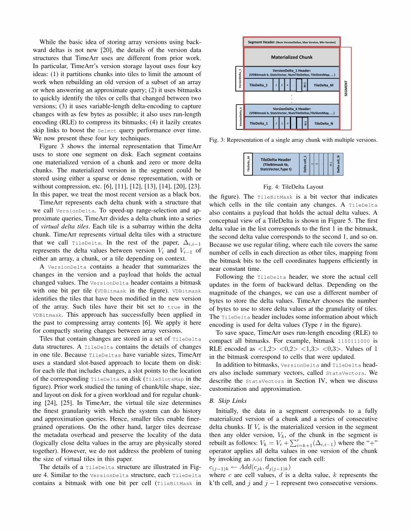
Figure 3 shows the internal representation that TimeArruses to store one segment on disk. Each segment containsone materialized version of a chunk and zero or more deltachunks. The materialized version in the segment could bestored using either a sparse or dense representation, with orwithout compression, etc. [6], [11], [12], [13], [14], [20], [23].In this paper, we treat the most recent version as a black box.

TimeArr represents each delta chunk with a structure thatwe call VersionDelta. To speed-up range-selection and ap-proximate queries, TimeArr divides a delta chunk into a seriesof virtual delta tiles. Each tile is a subarray within the deltachunk. TimeArr represents virtual delta tiles with a structurethat we call TileDelta. In the rest of the paper, ∆i,i−1

represents the delta values between version Vi and Vi−1 ofeither an array, a chunk, or a tile depending on context.

A VersionDelta contains a header that summarizes thechanges in the version and a payload that holds the actualchanged values. The VersionDelta header contains a bitmaskwith one bit per tile (VDBitmask in the figure). VDBitmask

identifies the tiles that have been modified in the new versionof the array. Such tiles have their bit set to true in theVDBitmask. This approach has successfully been applied inthe past to compressing array contents [6]. We apply it herefor compactly storing changes between array versions.

Tiles that contain changes are stored in a set of TileDelta

data structures. A TileDelta contains the details of changesin one tile. Because TileDeltas have variable sizes, TimeArruses a standard slot-based approach to locate them on disk:for each tile that includes changes, a slot points to the locationof the corresponding TileDelta on disk (TileSlotsMap in thefigure). Prior work studied the tuning of chunk/tile shape, size,and layout on disk for a given workload and for regular chunk-ing [24], [25]. In TimeArr, the virtual tile size determinesthe finest granularity with which the system can do historyand approximation queries. Hence, smaller tiles enable finer-grained operations. On the other hand, larger tiles decreasethe metadata overhead and preserve the locality of the data(logically close delta values in the array are physically storedtogether). However, we do not address the problem of tuningthe size of virtual tiles in this paper.

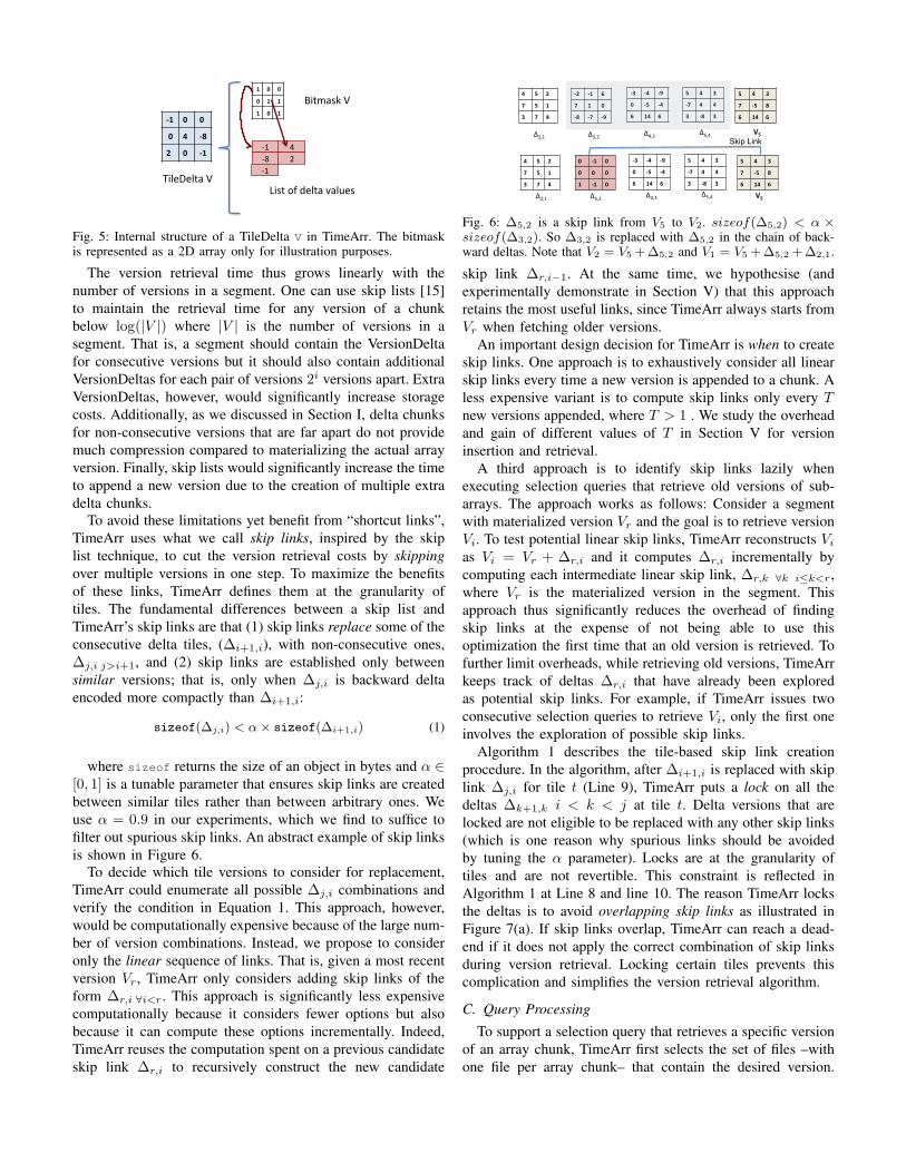
The details of a TileDelta structure are illustrated in Fig-ure 4. Similar to the VersionDelta structure, each TileDelta

contains a bitmask with one bit per cell (TileBitMask in

VersionDelta_1  Header:    (VDBitmask  b,  StatsVector,  NumTileDeltas,  TileSlotsMap,  …  )  

TileDelta_1   TileDelta_M  2   3   4  

Materialized  Chunk  

.   M-­‐1  

.  

VersionDelta_k  Header:  (VDBitmask  b,  StatsVector,  NumTileDeltas,TileSlotsMap,  …  )  

TileDelta_1   TileDelta_N  2   3   4   .  .  

Segment  Header:  (Num  VersionDeltas,  Max  Version,  Min  Version)  

VersionD

elta_1  

VersionD

elta_k  

N-­‐1  

SEGMEN

T  

Fig. 3: Representation of a single array chunk with multiple versions.

TileDelta  Header  (TileBitmask  tb,    

StatsVector,Type  t)     Delta

 cell_1  

2    

TileDe

lta_M

 

Delta

 cell_N  

3    

.    

.    

N-­‐1

   

Fig. 4: TileDelta Layout

the figure). The TileBitMask is a bit vector that indicateswhich cells in the tile contain any changes. A TileDelta

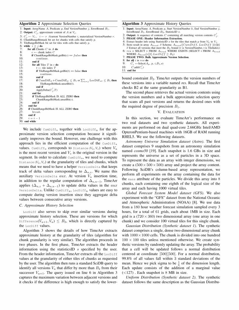
also contains a payload that holds the actual delta values. Aconceptual view of a TileDelta is shown in Figure 5. The firstdelta value in the list corresponds to the first 1 in the bitmask,the second delta value corresponds to the second 1, and so on.Because we use regular tiling, where each tile covers the samenumber of cells in each direction as other tiles, mapping fromthe bitmask bits to the cell coordinates happens efficiently innear constant time.

Following the TileDelta header, we store the actual cellupdates in the form of backward deltas. Depending on themagnitude of the changes, we can use a different number ofbytes to store the delta values. TimeArr chooses the numberof bytes to use to store delta values at the granularity of tiles.The TileDelta header includes some information about whichencoding is used for delta values (Type t in the figure).

To save space, TimeArr uses run-length encoding (RLE) tocompact all bitmasks. For example, bitmask 1100111000 isRLE encoded as <1,2> <0,2> <1,3> <0,3>. Values of 1in the bitmask correspond to cells that were updated.

In addition to bitmasks, VersionDelta and TileDelta head-ers also include summary vectors, called StatsVectors. Wedescribe the StatsVectors in Section IV, when we discusscustomization and approximation.

B. Skip Links

Initially, the data in a segment corresponds to a fullymaterialized version of a chunk and a series of consecutivedelta chunks. If Vr is the materialized version in the segmentthen any older version, Vk, of the chunk in the segment isrebuilt as follows: Vk = Vr+

∑ri=k+1(∆i,i−1) where the “+”

operator applies all delta values in one version of the chunkby invoking an Add function for each cell:c(j−1)k ← Add(cjk, dj(j−1)k)where c are cell values, d is a delta value, k represents thek’th cell, and j and j − 1 represent two consecutive versions.

TileDelta  V  

1 0 0

0 1 1

1 0 1-­‐1   0   0  

 0   4   -­‐8  

2   0   -­‐1  -­‐1   4  -­‐8   2  -­‐1  

Bitmask  V  

List  of  delta  values  

Fig. 5: Internal structure of a TileDelta V in TimeArr. The bitmaskis represented as a 2D array only for illustration purposes.

The version retrieval time thus grows linearly with thenumber of versions in a segment. One can use skip lists [15]to maintain the retrieval time for any version of a chunkbelow log(|V |) where |V | is the number of versions in asegment. That is, a segment should contain the VersionDeltafor consecutive versions but it should also contain additionalVersionDeltas for each pair of versions 2i versions apart. ExtraVersionDeltas, however, would significantly increase storagecosts. Additionally, as we discussed in Section I, delta chunksfor non-consecutive versions that are far apart do not providemuch compression compared to materializing the actual arrayversion. Finally, skip lists would significantly increase the timeto append a new version due to the creation of multiple extradelta chunks.

To avoid these limitations yet benefit from “shortcut links”,TimeArr uses what we call skip links, inspired by the skiplist technique, to cut the version retrieval costs by skippingover multiple versions in one step. To maximize the benefitsof these links, TimeArr defines them at the granularity oftiles. The fundamental differences between a skip list andTimeArr’s skip links are that (1) skip links replace some of theconsecutive delta tiles, (∆i+1,i), with non-consecutive ones,∆j,i j>i+1, and (2) skip links are established only betweensimilar versions; that is, only when ∆j,i is backward deltaencoded more compactly than ∆i+1,i:

sizeof(∆j,i) < α× sizeof(∆i+1,i) (1)

where sizeof returns the size of an object in bytes and α ∈[0, 1] is a tunable parameter that ensures skip links are createdbetween similar tiles rather than between arbitrary ones. Weuse α = 0.9 in our experiments, which we find to suffice tofilter out spurious skip links. An abstract example of skip linksis shown in Figure 6.

To decide which tile versions to consider for replacement,TimeArr could enumerate all possible ∆j,i combinations andverify the condition in Equation 1. This approach, however,would be computationally expensive because of the large num-ber of version combinations. Instead, we propose to consideronly the linear sequence of links. That is, given a most recentversion Vr, TimeArr only considers adding skip links of theform ∆r,i ∀i<r. This approach is significantly less expensivecomputationally because it considers fewer options but alsobecause it can compute these options incrementally. Indeed,TimeArr reuses the computation spent on a previous candidateskip link ∆r,i to recursively construct the new candidate

-­‐3   -­‐4   -­‐9  

0   -­‐5   -­‐4  

6   14   6  

-­‐2   -­‐1   6  

7   1   0  

-­‐8   -­‐7   -­‐9  

4   5   2  

7   5   1  

3   7   4  

5   4   3  

-­‐7   4   4  

3   -­‐8   3  

5   4   3  

7   -­‐5   8  

6   14   6  

V5  Δ5,4  Δ4,3  Δ3,2  Δ2,1  

 

-­‐3   -­‐4   -­‐9  

0   -­‐5   -­‐4  

6   14   6  

4   5   2  

7   5   1  

3   7   4  

5   4   3  

-­‐7   4   4  

3   -­‐8   3  

5   4   3  

7   -­‐5   8  

6   14   6  

V5  Δ5,4  Δ4,3  Δ5,2  Δ2,1  

0   -­‐1   0  

0   0   0  

1   -­‐1   0  

Skip Link

Fig. 6: ∆5,2 is a skip link from V5 to V2. sizeof(∆5,2) < α ×sizeof(∆3,2). So ∆3,2 is replaced with ∆5,2 in the chain of back-ward deltas. Note that V2 = V5 + ∆5,2 and V1 = V5 + ∆5,2 + ∆2,1.

skip link ∆r,i−1. At the same time, we hypothesise (andexperimentally demonstrate in Section V) that this approachretains the most useful links, since TimeArr always starts fromVr when fetching older versions.

An important design decision for TimeArr is when to createskip links. One approach is to exhaustively consider all linearskip links every time a new version is appended to a chunk. Aless expensive variant is to compute skip links only every Tnew versions appended, where T > 1 . We study the overheadand gain of different values of T in Section V for versioninsertion and retrieval.

A third approach is to identify skip links lazily whenexecuting selection queries that retrieve old versions of sub-arrays. The approach works as follows: Consider a segmentwith materialized version Vr and the goal is to retrieve versionVi. To test potential linear skip links, TimeArr reconstructs Vias Vi = Vr + ∆r,i and it computes ∆r,i incrementally bycomputing each intermediate linear skip link, ∆r,k ∀k i≤k<r,where Vr is the materialized version in the segment. Thisapproach thus significantly reduces the overhead of findingskip links at the expense of not being able to use thisoptimization the first time that an old version is retrieved. Tofurther limit overheads, while retrieving old versions, TimeArrkeeps track of deltas ∆r,i that have already been exploredas potential skip links. For example, if TimeArr issues twoconsecutive selection queries to retrieve Vi, only the first oneinvolves the exploration of possible skip links.

Algorithm 1 describes the tile-based skip link creationprocedure. In the algorithm, after ∆i+1,i is replaced with skiplink ∆j,i for tile t (Line 9), TimeArr puts a lock on all thedeltas ∆k+1,k i < k < j at tile t. Delta versions that arelocked are not eligible to be replaced with any other skip links(which is one reason why spurious links should be avoidedby tuning the α parameter). Locks are at the granularity oftiles and are not revertible. This constraint is reflected inAlgorithm 1 at Line 8 and line 10. The reason TimeArr locksthe deltas is to avoid overlapping skip links as illustrated inFigure 7(a). If skip links overlap, TimeArr can reach a dead-end if it does not apply the correct combination of skip linksduring version retrieval. Locking certain tiles prevents thiscomplication and simplifies the version retrieval algorithm.

C. Query Processing

To support a selection query that retrieves a specific versionof an array chunk, TimeArr first selects the set of files –withone file per array chunk– that contain the desired version.

Algorithm 1 Skip Links Creation Procedure for One Tile1: Input: Materialized Version Vr , Delta versions ∆i+1,i, Target Version Index k.2: Output: Vk .3: i← r − 14: ∆r,x ← φ5: while i ≥ k do6: ∆r,x ← ∆r,x + ∆i+1,i

7: if ∆r,x ≤ (α×∆i+1,i) then8: if ∆i+1,i is not locked then9: Replace ∆i+1,i with ∆r,x

10: Lock all the ∆n+1,n i < n < r11: end if12: end if13: i = i− 114: end while15: Vk ← Vr + ∆r,x

Δ 10,9  

 V 10  

  Δ 9,8  

  Δ 8,7  

  Δ 7,6  

 Δ 1

0,5  

  Δ 5,4  

  Δ 4,3  

  Δ 2,1  

 Δ 8,2  

 

L10,5

L8,2

(a) Invalid State: V1 and V2 areaccessible only if TimeArr appliesL8,2 and not L10,5.

Δ 10,9  

 V 10  

  Δ 9,8  

  Δ 8,7  

  Δ 7,6  

  Δ 9,5  

  Δ 5,4  

 Δ 1

0,3  

  Δ 2,1  

 

Δ 10,2  

 

L10,3

L9,5

L10,2

(b) Valid State: All versions are acces-sible through any combination of links.

Fig. 7: Valid v.s. Invalid states of skip links. TimeArr must avoidoverlapping skip links. The lock mechanism prevents Invalid state(a) by prohibiting L10,5.

Within each file, TimeArr starts from the most recent mate-rialized chunk version and applies all the changes backwardsuntil it rebuilds the version of interest.

If the selection query includes a range predicate, TimeArrleverages its virtual tiles to identify and process only changesthat fall within the region of interest.

Each delta tile ∆j,j−1 keeps track of a constant number ofskip links ∆j,i j−1>i that TimeArr can leverage at version Vjto skip directly to an older version Vi. Each ∆j,j−1 storesthe number of versions that ∆j,i skips as Lji = (j − i − 1)as shown in Figure 7. In our experiments keeping track of asmall number of Lji’s, L = 3, sufficed to hold all skip linksfor α < 0.9. Right before applying ∆j,j−1, TimeArr checksfor potential skip links to leverage. TimeArr selects a linkthat skips the most versions while still landing before or atthe desired version. For example in Figure 7(b), in order toretrieve version V1, TimeArr chooses L10,2 = 7 at V10 andskips 7 delta tiles until it reaches ∆10,2 which means V1 =V10 + ∆10,2 + ∆2,1. These choices are performed separatelyfor each tile.

IV. APPROXIMATE QUERIES

In this section, we present TimeArr’s approach to efficientlysupporting approximate queries.

A. Distance between Versions

We recall from Section II that, when a user requests theapproximate content c′j(p) of the subarray satisfying predicatep at version number j, the user specifies the maximumtolerable error in the form of an error bound B1. The systemguarantees that the data returned will satisfy the conditionDifference(c′j(p), cj(p)) < B1. The difference between twosubarrays can be computed at the granularity of tiles or chunksas requested by the user. The semantics are as follows:

Listing 1 Distance Function at the Granularity of Tiles// A1 and A2 are two versions of the same tiledouble Distance (Subarray A1, Subarray A2)Instantiate Statistics object s.s.initialize()Iterate over all pairs of matching cells (c1,c2)where c1 in A1 and c2 in A2 in lock step:

delta = s.subtract(c1,c2)s.process(delta)

return s.finalize()

Listing 2 Distributive Distance Function at the Granularity ofChunks// A1 and A2 are two versions of the same chunkdouble Distance (Subarray A1, Subarray A2)Instantiate Statistics object s.s.initialize()Iterate over all pairs of matching tiles t1 and t2 wheret1 in A1 and t2 in A2 in lock step:

delta = Distance(t1,t2)s.merge(delta)

return s.finalize()

Difference(c′j(p), cj(p)) < B1 iff (2)

∀tiles or chunks c′jk ∈ c′j Distance(c′jk, cjk) < B1

where cj(p) is the exact content of the subarray at versionj and cjk(p) is the exact content of tile or chunk k inthat subarray. The computation includes tiles or chunks thatpartially overlap the subarray cj(p).

Similarly, the Difference between subarrays is equal to B1

if the Distance between all pairs of tiles or chunks is equalto B1. If the Difference is neither less than B1 nor equal toB1, then it is considered to be greater than B1.

Distance functions in TimeArr are implemented in amanner analogous to aggregation functions in OLAP datacubes [26] or parallel aggregations [27]. The distance betweentwo tiles is computed by aggregating the delta values of theircells as shown in Listing 1: the Distance function takes twoversions of the same tile as input (A1 and A2). It iterates overthe two versions and computes the delta value for each pair ofcells. The subtract method used here is the same as the oneintroduced in Section III. It then accumulates these differencesusing a standard aggregation method.

If the difference computation is at the granularity of chunks,to avoid tedious re-computations, TimeArr requires that theDistance function be distributive as defined by Gray etal. [26]: max(), count(), and sum() are all distributive. That is,to compute the Distance of two chunks, TimeArr aggregatesthe Distance of the underlying tiles as shown in Listing 2.

The user can redefine the subtract and aggregate operationsinvolved in these distance computations as we describe shortly.

TimeArr also requires the Distance function to be a metricand thus to satisfy the triangle inequality:

Distance(A1, A3) ≤ Distance(A1, A2) +Distance(A2, A3) (3)

where Ai is a subarray. An example of a metric is aDistance function that computes the maximum delta valuefor all cells in the array.

At the core of these Distance functions is the Statistics

object, which defines how the delta values are computed

Listing 3 Statistics Interfaceinterface StatisticsCellValue add (CellValue, CellValue)CellValue subtract(CellValue, CellValue)

void initialize()process(CellValue c)merge(Statistics s2)double finalize()

and aggregated. To implement a new Distance function, auser only needs to provide a new class that implements theStatistics interface as shown in Listing 3.

The add and subtract methods operate on delta values asdescribed in Section III. CellValue can be any numeric atomictype including integer and real.

TimeArr allows users to provide multiple classes thatimplement the Statistics interface. TimeArr also provides adefault Distance function using a default Statistics classthat computes a value difference for subtract and a valuesum for add. It also maintains the absolute maximum deltavalue across versions as the aggregate distance returned byfinalize.

Next, we present how TimeArr uses these Distance func-tions to answer approximate queries.

B. Approximate Version Selection

Given a segment with a fully materialized chunk version Vrand VersionDeltas for earlier versions Vr−1 down to Vz (theoriginal version in the segment), the goal is to return somedesired version Vj within an error bound B1.

In the absence of approximation, TimeArr will start withVr and it will apply delta chunks in sequence (using skip-links when possible) until it gets back to version Vj . Withapproximation specified at the granularity of tiles, for eachtile separately, we want to stop the delta application process assoon as we reach a version V ′j that satisfies the error condition:Distance(cj′k, cjk) < B1, where cjk is the content of tilek at version j and cj′k is the content of that same tile atversion j′. If the approximation is specified at the granularityof chunks, TimeArr returns a set of tiles in the approximatechunk cj′k that all have the same version j

′and it checks the

error condition at the granularity of the whole chunk.The key question is how to efficiently verify these error

conditions? It is impractical to compute the Distance func-tion between all versions of each tile in a chunk. Instead,TimeArr computes only two distances for each version Vu:Distance(cuk, cu−1,k) and Distance(cuk, czk). We call theformer distance the LocDiffuk or Local Difference at versionu and tile index k because it is a difference between consec-utive versions . We call the latter distance the CumDiffuk orCumulative Difference at version u and tile index k becauseit is the distance to the oldest version in the chunk.

For each new version Vu appended to a chunk, TimeArrcomputes CumDiffuk and LocDiffuk at the granularity oftiles and stores the results in the TileDelta StatsVector forversion Vu−1 (since version Vu will be materialized). Figure 8illustrates the CumDiff and LocDiff computation for a small

5   4   3  

7   -­‐5   8  

6   14   6  

-­‐1   0   0  

 0   10   -­‐8  

-­‐3   -­‐8   -­‐1  

0   1   -­‐2  

0   -­‐4    1  

-­‐3   -­‐6   -­‐4  

V3   Δ3,2   Δ2,1  

14    CD3  

LD3  

10   6  CD2  

LD2  

6  

Fig. 8: A 3x3 array with 3 versions. V3 is materialized and V2 andV1 are backward delta encoded. CumDiff (CD) and LocDiff (LD) arecalculated for the two ∆3,2 and ∆2,1. Highlighted cells are the onesto contribute to the CD and LD calculations, which use the defaultdistance (maximum absolute difference between any two cells). TheVersionDelta for ∆3,2 contains CumDiff3 and LocDiff3. Similarly,the VersionDelta for ∆2,1 contains CumDiff2 and LocDiff2.

array. Finally, TimeArr merges these CumDiff and LocDiff

values for all tiles in a chunk and stores the chunk-levelCumDiff and LocDiff in the VersionDelta StatsVector.

Hence, the StatsVector is a vector of pairs(CumDiff,LocDiff), with one pair for the system’s defaultStatistics object and extra pairs for all the user-definedStatistics objects. In the API in Table I, the arguments thatrefer to statistics are indexes into the StatsVector.

To verify that the error condition is satisfied, TimeArrleverages the fact that Distance is a metric and veri-fies two conditions. First, since CumDiffj′k is defined asDistance(cj′k,czk), and the distance function is a metric, wehave:

Distance(cj′k, cjk) ≤ CumDiffj′k + CumDiffjk (4)

Therefore:

IF CumDiffj′k + CumDiffjk ≤ B1 ⇒ Distance(cj′k, cjk) ≤ B1 (5)

Second, TimeArr performs a similar check using LocDiffs:

IF

jXu=j′

LocDiffuk ≤ B1 ⇒ Distance(cj′k, cjk) ≤ B1 (6)

If either condition holds, cj′k is an approximate version ofc′

jk that satisfies the error threshold B1, which avoids furtherprocessing of tile k until version Vj .

Algorithm 2 shows how TimeArr utilizes CumDiff andLocDiff in Equation 5 and 6 to answer approximate selectionqueries of the form: “Select version Vj of array A withpredicate p and ErrorBound B1”. For simplicity, the algo-rithm is only described for the error computation at the tilegranularity, but it follows a similar description for the chunkgranularity. For each tile, Algorithm 2 finds the version Vj′

that satisfies either of the inequalities in Equation 5 or 6.Then it reconstructs and updates C

′

j as the approximate versioncontent. It repeats the process for all the tiles separately.

Algorithm 2 uses two bitmasks ChunkRangeBitmask andTileRangeBitmask that keep track of the chunks and tiles thatrequire to be processed further toward version j. Wheneverthe CumDiff or the LocDiff of a given tile satisfies theinequality in Equation 5 or 6, respectively, the correspondingbit value in TileRangeBitMask is set to 0, which avoids furthertriggers of the ApplyDelta() function for the same tile. TheApplyDelta(cjk,C

′j) executes the Add() function on all the

corresponding pairs of cells in cjk and C′

j .

Algorithm 2 Approximate Selection Queries1: Input: ArrayName A, Predicate p, End VersionNumber j, ErrorBound B1.2: Output: C

′j , approximate content of A at Vj .

3: C′j ← Vr, i← r //current VersionNumber i, materialized VersionNumber r.

4: ChunkRangeBitmask bit set for chunks with cells that satisfy p.5: TileRangeBitMask bit set for tiles with cells that satisfy p.6: while i ≥ j do7: for all Chunks C in A do8: c← chunk index C9: if ChunkRangeBitMask.getBit(c) == false then

10: continue.11: end if12: for all Tiles T in c do13: t← tile index T14: if TileRangeBitMask.getBit(t) == false then15: continue.16: end if17: if CumDiffit+CumDiffjt ≤ B1 or

Piu=j LocDiffut ≤ B1 then

18: TileRangeBitMask.unsetBit(t).19: end if20: ApplyDelta(C

′j ,T )

21: end for22: if TileRangeBitMask IS ALL ZERO then23: ChunkRangeBitMask.unsetBit(c).24: end if25: end for26: if ChunkRangeBitMask IS ALL ZERO then27: break.28: end if29: i = i− 130: end while

We include CumDiffu together with LocDiffu for the ap-proximate version selection computation because it signifi-cantly improves the bound. However, one challenge with thisapproach lies in the efficient computation of the CumDiffu

values. CumDiffu corresponds to Distance(Vu, Vz) where Vuis the most recent version and Vz is the original version in thesegment. In order to calculate CumDiffu, we need to computeDistance(Vu, Vz) at the granularity of tiles and chunks, whichmeans that we need to have a helper VersionDelta that keepstrack of delta values corresponding to ∆u,z . We name thisauxiliary VersionDelta aux. At version Vu insertion time,in addition to the regular computation of ∆u,u−1, TimeArrapplies (∆u,z + ∆u,u−1) to update delta values in the auxVersionDelta. Unlike CumDiffu, LocDiffu values are easy tocompute during version insertion since they aggregate deltavalues between consecutive array versions.

C. Approximate History Selection

LocDiff also serves to skip over similar versions duringapproximate history selection. These are versions for whichDifference(Vu+1, Vu) ≤ B2, which is directly captured bythe LocDiff values.

Algorithm 3 shows the details of how TimeArr extractsapproximate history at the granularity of tiles (algorithm forchunk granularity is very similar). The algorithm proceeds intwo phases. In the first phase, TimeArr extracts the headerinformation using the statisticsID s specified by the user.From the header information, TimeArr extracts all the LocDiff

values at the granularity of either tiles of chunks as requestedby the user. The algorithm then runs a standard SciDB query toidentify all versions Vu that differ by more than B2 from theirsuccessor Vu+1. The query issued on line 6 in Algorithm 3captures the maximum variation between adjacent versions andit checks if the difference is high enough to satisfy the lower-

Algorithm 3 Approximate History Queries1: Input: ArrayName A, Predicate p, Start VersionNumber k, End VersionNumber j,

ErrorBound B1, ErrorBound B2, StatisticID s.2: Output: A sequence of contents C containing all matching version contents C

′j .

3: PHASE ONE: Header Information Extraction.4: Extract header info using StatisticID s for the tiles that match p from Vk to Vj .5: Store result in array Ahead. // Schema: Ahead{CumDiff , LocDiff }[v][t]

// Extract all versions that meet the B2 bound (v is VersionNumber, t is TileIndex):6: res = SELECT v FROM Ahead WHERE EXISTS (SELECT t FROM Ahead

WHERE Ahead[v][t].LocDiff ≥ B2)7: PHASE TWO: Bulk Approximate Version Selection.8: for all i in res do9: C

′i ←Select(Ap, p, i,B1,s)

10: C.add(C′i )

11: end for

bound constraint B2. TimeArr outputs the version numbers ofthese versions into a variable named res. Recall that TimeArrchecks B2 at the same granularity as B1.

The second phase retrieves the actual version contents usingthe version numbers and a bulk approximate selection querythat scans all past versions and returns the desired ones withthe required degree of precision B1.

V. EVALUATION

In this section, we evaluate TimeArr’s performance ontwo real datasets and two synthetic datasets. All experi-ments are performed on dual quad-core 2.66GHz Intel/AMDOpteronPentium-based machines with 16GB of RAM runningRHEL5. We use the following datasets.

Astronomy Universe Simulation dataset (Astro). The firstdataset comprises 9 snapshots from an astronomy simulationnamed cosmo50 [19]. Each snapshot is 1.6 GBs in size andrepresents the universe as a set of particles in a 3D space.To represent the data as an array with integer dimensions, wecreate a (500×500×500) array and project the array content.Following SciDB’s column-based array representation, weperform all experiments on the array containing the data forthe mass attribute of the particles. We divide this array into 8chunks, each containing one eighth of the logical size of thearray and each having 1000 virtual tiles.

Global Forecast System Model dataset (GFS). We alsoexperiment with the “GFS” dataset from the National Oceanicand Atmospheric Administration (NOAA) [8]. We use datafrom a 180 hour weather forecast simulation sampled every 3hours, for a total of 61 grids, each about 1MB in size. Eachgrid is a (720× 360) two dimensional array (one array in onechunk) and we consider 100 virtual tiles for this single chunk.

Gaussian Distribution (Synthetic dataset 1). The syntheticdataset comprises a single, dense two-dimensional array chunkwith 1000×1000 cells. The chunk is divided into one hundred100 × 100 tiles unless mentioned otherwise. We create syn-thetic versions by randomly updating the array. The probabilitythat a cell will be updated follows a normal distributioncentered at coordinate [500][500]. For a normal distribution,99.8% of all values fall within 3 standard deviations of themean. Hence we pick sigma to be 1

6 of the dimension length.Each update consists of the addition of a marginal value(<127) . Each snapshot is 8 MB in size.

Uniform Distribution (Synthetic dataset 2). The syntheticdataset follows the same description as the Gaussian Distribu-

0  

1  

2  

3  

4  

1   6   11   16   21   26   31   36   41   46   51   56   61   66   71   76   81   86   91   96  

Version  Crea5o

n  Time  (Secon

ds)  

 

Version  Number    

Synthe5c  Dataset  1:  Time  to  Create  Version  

I/O  %me   Whole  %me  

I/O  %me  Approx   Whole  %me  Approx    

Fig. 9: Time to create 100 versions of a two-dimensional array withnormally distributed updates. A new segment is initialized at version65 in the non-approximate setting and version 62 when approxima-tions are enabled. Each new version adds a constant overhead. I/Ooverhead is insignificant.

0.38  

0.49  

1.02  

1.37  

0  

0.2  

0.4  

0.6  

0.8  

1  

1.2  

1.4  

1.6  

60   55   50   45   40   35   30   25   20   15   10   5   0  

Version  Fetch  Time  (Secon

ds)  

Version  Number  

GFS  Dataset:  Time  to  Fetch  Version  

approx1(2β)   approx2(β)   approx3(β/2)   no-­‐approx  

Fig. 10: Time to fetch each version in the GFS dataset. β, 2β, and β2

refer to the error bounds, where β is the average maximum changeobserved in two adjacent versions. I/O times are insignificant and notshown. For the GFS dataset the maximum segment size is 12 MBs.The segments reaches its full size at version number 38 and 36 inthe non-approximate and approximate settings respectively.

tion except the probability that a cell will be updated followsa uniform distribution.A. Basic Version Creation and Retrieval Performance

We first evaluate the performance when appending newversions to an array. Figure 9 shows the time to create100 new versions for the first synthetic dataset. Each newversion adds a constant overhead (1.5 seconds) in the non-approximate setting. The overhead is constant primarily be-cause the total number of updates is approximately the samefor each version. As we show later, the version creation timegrows almost linearly with the number of updated cells perversion. The overhead of creating a new version is higher withapproximation enabled. The extra overhead comes primarilyfrom updating the aux VersionDelta in addition to the mainVersionDelta, doubling processing times. The I/O times inboth cases are insignificant. The CPU cost of computing deltavalues dominates the runtime. In this experiment, we arbitrar-ily set the segment size to 48 MBs. When a new segmentis created the version creation time with approximation isclose to the non-approximate setting primarily because the auxVersionDelta starts-off empty and is thus quick to update. Weobserve the same trend with the real datasets, not shown dueto space constraints, but available in our technical report [28].

Next, we study the query processing time to fetch eachversion either precisely or approximately in synthetic and realdatasets. For the experiments with approximation, we consideran error bound β equal to the average maximum changeobserved between any two adjacent versions. With such an

error bound, the user may see values that are in aggregate offby at most one array version. As Figure 10 shows, the costof retrieving a version precisely decreases linearly with theversion number. With high approximation (error bound β), forthe GFS dataset, query times decrease by factors between 25%and 300%. Similarly, we observed that retrieving any versionin the synthetic dataset (not shown in the figure) takes half thetime or less compared with retrieving the exact version. Evenwith a small approximation (error bound β/2), performancegains are above 35%. We observed similar trends for the Astro

dataset (not shown).Overall, TimeArr’s approach to approximate query pro-

cessing thus adds overhead during version insertion. Thisoverhead, however, is paid only once. At the same time,approximation enables the system to cut query times signif-icantly when users can tolerate approximate results. Thesesavings are repetitive. Interestingly, the performance gains ofapproximation increase as we query older versions while theversion creation overhead remains constant.

We also studied the effect of the number of updates on theversion creation time. We calculated the total time to create50 versions from the synthetic dataset 2 with differentnumbers of updates ranging from one thousand to one millionupdates per version. As expected version creation time growsalmost linearly with the number of updates per version. Goingfrom one thousand to one million updates always added 7to 8 seconds to the total version creation time. We did asimilar experiment keeping the number of updates constant,but increasing the updated values. We observed no significantincrease in the version creation time (although the size of theversion in terms of bytes changed rapidly). We do not showgraphs of those experiments due to space constraints.

We also evaluated the benefit of using virtual tiles andvariable-length delta encoding on the storage space at versioncreation time and we observed up to 70% space savingscompare to the case with no-tile settings and no variable-lengthdelta encoding. The space savings, however, do not come forfree. The finest tile settings in the experiment had up to 25%version creation time overhead compare to the no-tile settings.

We now evaluate the benefits of using virtual tiles to speed-up historical queries over subsets of a chunk (i.e., rangeselection queries over array coordinates). Figure 11 shows theperformance of the following query: Return the original

version of the rectangular subarray [C1;C2], where C1

and C2 are the upper-left and lower-right corners of a region.In Figure 11(a), we use a single chunk with 100 virtual tilesand Synthetic dataset 1. The rectangular regions have the samecenter as the chunk and range from one tile to the wholechunk. The performance gains that we achieve using virtualtiles depend on the granularity of the tiles and the size of thefetched region. In the tile setting in this experiment, we fetch asingle tile 50 times faster than the setting with no virtual tilesused. Even with the window sizes that retrieve as much as 25%of the chunk, TimeArr runs significantly faster than the settingwithout virtual tiles. Figure 11(b) shows the performance ofthe range selection query on the astronomy dataset. Similar

(a)

0  

0.5  

1  

1.5  

2  

2.5  

0  

0.0025  

0.01  

0.0225  

0.04  

0.0625  

0.09  

0.1225  

0.16  

0.25  

0.3025  

0.36  

0.4225  

0.49  

0.5625  

0.64  

0.7225  

0.81  

0.9025   1  O

riginal  Version

 Fetch  Tim

e  (Secon

ds)  

PorCon  of  Chunk  Queried  

SyntheCc  Dataset  1:  Fetch  Original  Version  on  Different  Regions    

virtual  Cle   no  virtual  Cle  

(b)

0  

5  

10  

15  

20  

25  

30  

35  

0.000001  

0.001  

0.008  

0.027  

0.064  

0.125  

0.216  

0.343  

0.512  

0.729   1  O

riginal  Version

 Fetch  Tim

e  (Secon

ds)  

PorCon  of  Chunk  Queried  

Astronomy  Universe  Simulaton  :  Fetch  Original  Version  on  Different  Regions    

virtual  Cle   no  virtual  Cle  

Fig. 11: Time to fetch the original version where the region windowchanges from one tile to the whole chunk. (a) Synthetic dataset with20 versions. (b) Astronomy dataset with 9 versions.

to what we observed in the synthetic dataset, the benefits ofusing virtual tiles to speed-up historical queries over subsetsof an array are significant. The trend is the same for the GFSdataset as well.

B. Version Retrieval with Links Support

The advantage of the skip link technique is highlighted ondatasets such as the Global Forecast System Model (GFS)where similar data patterns are repeated at different versions.Figure 12 shows the time to fetch 60 versions of the GFSdataset. The segment size is chosen such that all the versionsreside in one segment. In this experiment, TimeArr period-ically computes skip links after each T versions appended.As illustrated in Figure 12 the performance gain to fetchthe oldest version with skip links is 42% for T = 20 and75% for T = 1 compared to the no-link case. However, theskip link computation incurs overhead at version insertiontime. Table II summarizes the overhead for different valuesof T . Although exhaustive computation of skip links (T = 1)improves the performance in Figure 12, it incurs significantoverhead when inserting new versions. Finding the optimalinterval T is left for future work. Instead, TimeArr useslazy computation of skip links whose performance is shownin Figure 13. The query workloads, Q-NORM and Q-UNIFORM

are as follows: TimeArr appends 61 versions from the GFSdataset in total and between each append operation, we issue5 original-version retrieval queries (305 queries in total). Eachoriginal-version retrieval query only fetches a few tiles fromthe array. The tiles to be fetched are selected randomly basedon either normal distribution (Q-NORM) or uniform distribution(Q-UNIFORM). Figure 13(a) shows the advantage of the lazylink computation with the Q-NORM workload. Q-NORM simulatesa workload with a hot spot region; i.e., a number of tiles arefetched many times while other tiles are fetched only once.Figure 13(a) shows that lazy computation of skips links isbetter than the skip-link computation at version insertion time

2.17  

1.52  

1.24  

1.01  

0  

0.5  

1  

1.5  

2  

60   55   50   45   40   35   30   25   20   15   10   5   0  

Version  Fetch  Time  (Secon

ds)  

Version  Number  

GFS  Dataset:  Time  to  Fetch  Versions  

SKIP  LINK  (T=1)   SKIP  LINK  (T=20)   NO-­‐LINK   APPROX  

Fig. 12: Time to fetch each version in a single-chunk array with 60versions. The result with skip link is competitive with approximateresult with β error bound.

NoLink (Lazy) Link (T=20) Link (T=5) Link (T=1)Add Versions (sec) 13.16 12.00 13.48 14.56Create Links (sec) 0 3.68 11.11 47.13

TABLE II: GFS dataset: Skip links overhead at version insertion time.TimeArr computes skip links each T consecutive versions appended.

with interval T = 5. However, this is not true when TimeArrruns the Q-UNIFORM workload (Figure 13(b)), because the skip-link computation overhead for a specific tile at version fetchtime is not paid off later. In the Q-UNIFORM workload, manytiles are only fetched once. In Figure 13, lazy computationof skip links during version retrieval incurs approximately 2seconds of overhead in total (not shown in the figure). Thealgorithm to decide when to compute skip links lazily duringversion retrieval, when to compute them after certain intervalsat version insertion time, and possibly the combination of thesetwo approaches are left for future work.

C. Comparison with SciDB

The current SciDB version storage also uses backwardsdeltas [20]. Unlike TimeArr, however, it represents eachVersionDelta using two chunks, one with a sparse and theother with a dense representation. Each cell-value in theVersionDelta is either in the sparse or dense chunk.

We compare TimeArr to SciDB’s current storage managerusing the synthetic dataset 2. There is thus a total of 106

cells in a single-chunk array. We create four synthetic streamsof versions: mass updates, medium updates, rare updates,and very rare updates that correspond to 106,105,104, and103 updates between each array version respectively. Theapproximation feature is turned off in all the experiments.Table III shows the results. TimeArr outperforms SciDB in allfour cases. It achieves 40% version creation time savings formedium and mass updates. Table III also shows that versioncreation time variation in SciDB is much larger than TimeArrin the case of medium and mass updates. In TimeArr theoverhead of adding a new version is constant while this isnot the case in SciDB.

Figure 14 shows the query processing performance of bothapproaches when fetching the whole chunk at a specific,precise version. The chunk has 100 tiles. TimeArr achieves a1.6X to 6.6X performance gain in terms of query processingcompared with SciDB for mass and medium updates. Forrare updates, improvement is marginal (it is not shown in

0  

5  

10  

15  

20  

1   51   101   151   201   251   301  

Total  Tim

e  (Secon

ds)  

Number  of  Queries  

Cumula=ve  Cost  of  Running  Q-­‐NORM  

SKIP  LINK  LAZY   SKIP  LINK  (T=5)  

(a)

0  

5  

10  

15  

20  

25  

1   51   101   151   201   251   301  Total  Tim

e  (Secon

ds)  

Number  of  Queries  

Cumula=ve  Cost  of  Running  Q-­‐UNIFORM  

 SKIP  LINK  LAZY   SKIP  LINK  (T=5)  

(b)

Fig. 13: Cumulative query runtime of workloads Q-NORM andQ-UNIFORM. Skip links are computed either lazily at version retrievalor at version insertion time after each T = 5 versions appended.

updates mass medium rare very rareTimeArr (sec) AVG 1.16 0.60 0.50 0.48TimeArr (sec) STD 0.08 0.01 0.04 0.05

SciDB(sec) AVG 1.80 1.01 0.67 0.55SciDB(sec) STD 0.83 0.45 0.85 0.60

TABLE III: Average time to create one version after appending50 versions on a two-dimensional array with uniformly distributedupdates. TimeArr outperforms SciDB in all four cases.

the figure). TimeArr’s performance gains compared to SciDBcome from the fact that SciDB stores delta values in onedense and one sparse chunk for compactness. When fetchinga version, SciDB first needs to combine delta values fromboth representations, which incurs significant overhead. Also,TimeArr uses bitmask techniques to locate changes efficiently,while SciDB needs to iterate over the whole dense deltachunk. Overall, our design decision to have a single storagerepresentation for delta chunks is a key factor for TimeArr’squery time performance.

We also studied the advantage of using virtual tiles inTimeArr compared to the current implementation of SciDB.We did a similar experiment as the one in Figure 11. Weobserved two orders of magnitude improvement in TimeArrfor regions covering only a few tiles (Figure is not shown dueto space constraint. The trend is similar to Figure 11).

D. Approximate History Query

We now demonstrate the benefits of approximate historyquery using the GFS dataset. We execute the following ex-ample query: Select(AGFS,true,V1,V61,54,260) where Ainis the input array. This query asks for all 61 versions of thedataset such that each version is approximately returned withthe error bound B1 = 54 and only versions that differ byat least error bound B2 = 260 are returned. 260 is approxi-mately half of the maximum change observed in two adjacentversions. Figure 15 shows the result of this query. TimeArrquickly identifies that only 9 versions differ by more than thespecified threshold and it only requests to approximately fetchthese 9 versions. In contrast, with exact history TimeArr hasto fetch all the versions. The approximate query runs in lessthan 7.5 seconds and the equivalent precise query takes 37seconds to complete, which is a 5X performance difference.

VI. RELATED WORK

Delta encoding is a popular technique in video and imagecompression. Video compression codecs like MPEG-1 [29]

6.00  

1.48  

9.88  

0  

2  

4  

6  

8  

10  

12  

49   47   45   43   41   39   37   35   33   31   29   27   25   23   21   19   17   15   13   11   9   7   5   3   1  

Version  Fetch  Time  (Secon

ds)  

Version  number  

SyntheAc  Dataset  2:  Fetch  50  versions  (Timearr  vs.  SciDB)  

mass  updates(Timearr)   medium  updates(Timearr)  

rare  updates(Timearr)   very  rare  updates  (Timearr)  

mass  &  medium  updates  (SciDB)  

Fig. 14: Time to fetch each version from 1 to 50 on a two-dimensionalarray with uniformly distributed updates. TimeArr is about 1.6X to6.6X better than SciDB for mass and medium updates. “Rare updates”and “very rare updates” lines overlap for both systems. Only TimeArris shown.

260  

0  

100  

200  

300  

400  

500  

600  

1   6   11   16   21   26   31   36   41   46   51   56  

Aggreggated    Local  Differen

ce    

Version  Number  

GFS  Dataset:  Approximate  History  Query  

Exact  History   Approximate  History  

Fig. 15: Approximate history query returns only 9 versions out of61 with a maximum degree of changes from the previous versiongreater than 260, while in exact history , TimeArr has to go over allthe versions. The performance gain is almost 5X.

apply several delta encoding techniques both within and be-tween frames. Similar to TimeArr, they regularly materializeversions (frames) in a chain of delta frames, They also dividethe frames into smaller chunks and compare each chunk toevery possible region in a specified radius around its origin.Hence, their version insertion is expensive. Previous work [20]showed that although video compression techniques efficientlycompress arrays, the version import time is too expensive andconsequently not appropriate for versioning in array systems.

Most array engines being built today, such as Ras-DaMan [5], are not designed as no-overwrite storage sys-tems and consequently cannot naturally support versioning.NetCDF [30], [31] and HDF5 [32] are common data modelsthat provide a portable and efficient mechanism to store andaccess multidimensional data which are extensively used byscientists, but they also do not support versioning explicitly.

MOLAP [33] systems store data in multidimensional ar-rays [33], [34]. They focus on aggregation queries and exploitdata structures to efficiently compute rollups. The MOLAPsystem in [35] supports versions to represent changes to thedata sources that should be propagated to the data warehouseperiodically. But the versioning system is designed to benefitthe concurrency control mechanism in order to minimizecontention between query and maintenance transactions.

There is a long line of research on temporal databases [10],[36], [37], [38]. Temporal databases have two notions of time:“valid time” and “transaction time”. Many databases providetime-travel support along the transaction time dimension [9],

[10], [39], [40]. However, none of these databases is special-ized for time travel over array data nor approximate time-travel. In particular, Postgres [39] uses R-trees for versionmanagement. This technique is complementary to the approachthat we propose in this paper. Immortal DB [10] adds trans-action time database support into a database engine. For this,Immortal DB stores versions data as a linked list, while westore versions as delta values. Our versioning system alsoheavily applies array-oriented techniques including bitmasks,virtual tiles, and skip links. Finally, TimeArr supports a newtype of “approximate queries” in the context of scientific arraydatabase engines.

Version Control Systems are an old topic in computerscience. Versioning techniques such as forward and backwarddelta encoding and the use of multi-version B-trees have beenimplemented in various legacy systems. Git [41] is one ofthe conventional version-control systems and is believed to befaster and more disk efficient than other similar version-controlsystems. Our system borrows some ideas such as backwarddelta encoding from other version control systems such asGit, but we also use sophisticated array-oriented optimizationtechniques to efficiently encode the delta versions and tosupport approximate queries.

Lastly, the state of the art for versioning in array sys-tems [20] uses a materialization matrix to efficiently find thebest versions to materialize. We are similar to this recent priorwork [20] in the sense that we also use backward delta versionsand store and fetch consecutive deltas together. The ability ofour system to add skip links at the granularity of tiles, toapproximately answer queries, and our use of virtual tiles tosupport versioning at fine granularity are the main advantageof our system compared to this prior work [20].

VII. CONCLUSION

TimeArr is a new storage manager for an array database.Its key contribution is to efficiently store and retrieve versionsof an entire array or some sub-array. TimeArr also introducesthe idea of approximate exploration of an array’s history. Toachieve high performance, TimeArr relies on several tech-niques including virtual tiles, bitmask compression of changes,variable-length delta representations, and skip links. TimeArrenables users to customize their exploration by specifying boththe maximum degree of approximation tolerable and how itshould be computed. Experiments with a prototype implemen-tation on two real datasets demonstrate the performance ofTimeArr’s approach.

VIII. ACKNOWLEDGEMENTS

This work is partially supported by NSF grant IIS-1110370and the Intel Science and Technology Center for Big Data.

REFERENCES

[1] Large Synoptic Survey Telescope. http://www.lsst.org/.[2] Earth microbiome project. http://earthmicrobiome.org/.[3] Stonebraker et. al. Requirements for science data bases and SciDB. In

Fourth CIDR Conf. (perspectives), 2009.[4] Ballegooij et. al. Distribution rules for array database queries. In 16th.

DEXA Conf., pages 55–64, 2005.[5] Baumann et. al. The multidimensional database system RasDaMan. In

SIGMOD, pages 575–577, 1998.

[6] Rogers et. al. Overview of SciDB: Large scale array storage, processingand analysis. In Proc. of the SIGMOD Conf., 2010.

[7] Zhang et. al. RIOT: I/O-efficient numerical computing without SQL. InProc. of the Fourth CIDR Conf., 2009.

[8] National Oceanic and Atmospheric Administration. http://nomads.ncdc.noaa.gov/.

[9] Oracle Flashback Technology. (2005). http://www.oracle.com/technology/deploy/availability/htdocs/Flashback Overview.htm.

[10] Lomet, D. et. al. Transaction time support inside a database engine. InProc. of the 22nd ICDE Conf., 2006.

[11] Chang et. al. Titan: A high-performance remote sensing database. InICDE, pages 375–384, 1997.

[12] DeWitt et. al. Client-server paradise. In Proc. of the 20th VLDB Conf.,pages 558–569, 1994.

[13] Marathe et. al. Query processing techniques for arrays. The VLDBJournal, 11(1):68–91, 2002.

[14] Soroush, E. et. al. Arraystore: A storage manager for complex parallelarray processing. In Proc. of the SIGMOD Conf., 2011.

[15] Munro, J.I. et. al. Deterministic skip lists. In SODA ’92, 1992.[16] Graham Cormode, Minos N. Garofalakis, Peter J. Haas, and Chris

Jermaine. Synopses for massive data: Samples, histograms, wavelets,sketches. Foundations and Trends in Databases, 4(1-3):1–294, 2012.

[17] Joseph M. Hellerstein, Peter J. Haas, and Helen J. Wang. Onlineaggregation. In Proc. of the SIGMOD Conf., 1997.

[18] Vijayshankar Raman and Joseph M. Hellerstein. Partial results for onlinequery processing. In Proc. of the SIGMOD Conf., June 2002.

[19] Loebman et. al. Analyzing massive astrophysical datasets: CanPig/Hadoop or a relational DBMS help? In IASDS’09, 2009.

[20] Seering, A. et. al. Efficient versioning for scientific array databases. InProc. of the 28th ICDE Conf., 2012.

[21] Shimada et. al. A storage scheme for multidimensional data alleviatingdimension dependency. In ICDIM, pages 662–668, 2008.

[22] Chang, F. et. al. Bigtable: a distributed storage system for structureddata. In Proc. of the 7th OSDI Symp., 2006.

[23] Chang et. al. T2: a customizable parallel database for multi-dimensionaldata. SIGMOD Record, pages 58–66, 1998.

[24] Otoo et. al. Optimal chunking of large multidimensional arrays for datawarehousing. In Proc. of the 10th DOLAP Conf., pages 25–32, 2007.

[25] Sarawagi et. al. Efficient organization of large multidimensional arrays.In Proc. of the 10th ICDE Conf., pages 328–336, 1994.

[26] Gray, J. et. al. Data cube: A relational aggregation operator generalizinggroup-by, cross-tab, and sub-totals. Data Min. Knowl. Discov., pages29–53, 1997.

[27] Yu et. al. Distributed aggregation for data-parallel computing: interfacesand implementations. In Proc. of the 22st SOSP, 2009.

[28] Soroush, E. et. al. Time travel in a scientific array database. TechnicalReport UW-CSE-12-11-03, Department of Computer Science, Univer-sity of Washington, 2012.

[29] International Standards Organization (ISO), Coding of Moving Picturesand Audio. http://mpeg.chiariglione.org/standards/mpeg-1/mpeg-1.htm.

[30] The NetCDF Users’ Guide. http://www.unidata.ucar.edu/packages/netcdf/guidec/.

[31] Rew et. al. Data management: Netcdf: an interface for scientific dataaccess. IEEE Comput. Graph. Appl., 10(4):76–82, 1990.

[32] Introduction to HDF5. http://www.hdfgroup.org/HDF5/doc/H5.intro.html.

[33] P. M. Fernandez. Red brick warehouse: a read-mostly rdbms for opensmp platforms. Proc. of the SIGMOD Conf., pages 492–, 1994.

[34] Pedersen et. al. Multidimensional database technology. IEEE Computer,34(12):40–46, 2001.

[35] H.G. Kang and C.W Chung. Exploiting versions for on-line datawarehouse maintenance in molap servers. In Proc. of the 28th VLDBConf., pages 742–753, 2002.

[36] Ozsoyoglu, G. et. al. Temporal and real-time databases: A survey. IEEETKDE, pages 513–532, 1995.

[37] Jensen, C.S. et. al. Temporal data management. IEEE TKDE, pages36–44, 1999.

[38] R. Snodgrass and I. Ahn. A taxonomy of time databases. In Proc. ofthe SIGMOD Conf., pages 236–246, 1985.

[39] M. Stonebraker. The design of the postgres storage system. In Proc. ofthe 13th VLDB Conf., pages 289–300, 1987.

[40] L. Hobbs and K. England. Rdb: A Comprehensive Guide. Digital Press,1995.

[41] S. Chacon. the Git SCM community. http://book.git-scm.com/, 2010.